Section 2.10

Solid Mechanics Part III Kelly 279

2.10 Convected Coordinates An introduction to curvilinear coordinate was given in section 1.16, which serves as an introduction to this section. As mentioned there, the formulation of almost all mechanics problems, and their numerical implementation and solution, can be achieved using a description of the problem in terms of Cartesian coordinates. However, use of curvilinear coordinates allows for a deeper insight into a number of important concepts and aspects of, in particular, large strain mechanics problems. These include the notions of the Push Forward operation, Lie derivatives and objective rates. As will become clear, note that all the tensor relations expressed in symbolic notation already

discussed, such as CU , iii nNF ˆ , lFF , etc., are independent of coordinate system,

and hold also for the convected coordinates discussed here. 2.10.1 Convected Coordinates In the Cartesian system, orthogonal coordinates ,i iX x were used. Here, introduce the

curvilinear coordinates i . The material coordinates can then be written as

),,( 321 XX (2.10.1) so i

iX EX and

ii

ii ddXd GEX , (2.10.2)

where iG are the covariant base vectors in the reference configuration, with corresponding

contravariant base vectors iG , Fig. 2.10.1, with

ijj

i GG (2.10.3)

Section 2.10

Solid Mechanics Part III Kelly 280

Figure 2.10.1: Curvilinear Coordinates The coordinate curves form a net in the undeformed configuration (over the surfaces of constant i ). One says that the curvilinear coordinates are convected or embedded, that is, the coordinate curves are attached to material particles and deform with the body, so that each material particle has the same values of the coordinates i in both the reference and current configurations. The covariant base vectors are tangent the coordinate curves. In the current configuration, the spatial coordinates can be expressed in terms of a new, “current”, set of curvilinear coordinates

),,,( 321 t xx , (2.10.4) with corresponding covariant base vectors ig and contravariant base vectors ig , with

ii

ii ddxd gex , (2.10.5)

As the material deforms, the covariant base vectors ig deform with the body, being

“attached” to the body. However, note that the contravariant base vectors ig are not as such attached; they have to be re-evaluated at each step of the deformation anew, so as to ensure that the relevant relations, e.g. i i

j j g g , are always satisfied.

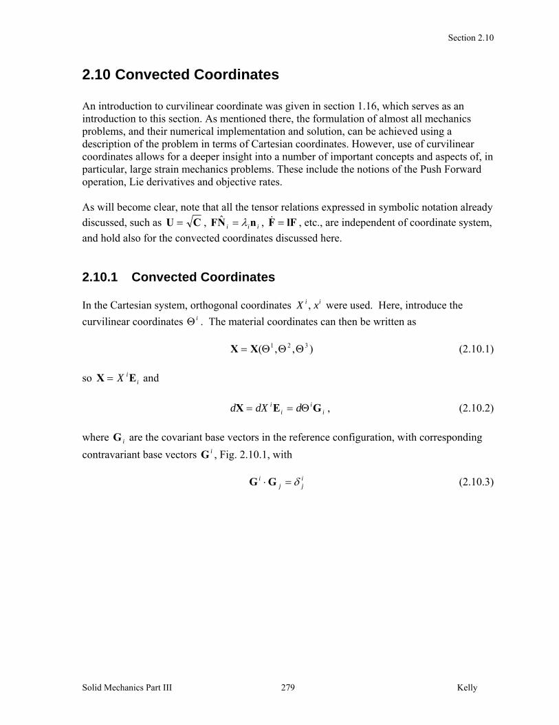
Example 1 Consider a pure shear deformation, where a square deforms into a parallelogram, as illustrated in Fig. 2.10.2. In this scenario, a unit vector 2E in the “square” gets mapped to a

vector 2g in the parallelogram1. The magnitude of 2g is 1 / sin .

1 This differs from the example worked through in section 1.16; there, the vector g2 maintained unit magnitude.

11, xX

22 , xX

33 , xX

X

11,eE

22 ,eE

1g2g

current configuration

reference configuration

1G2G

x

Section 2.10

Solid Mechanics Part III Kelly 281

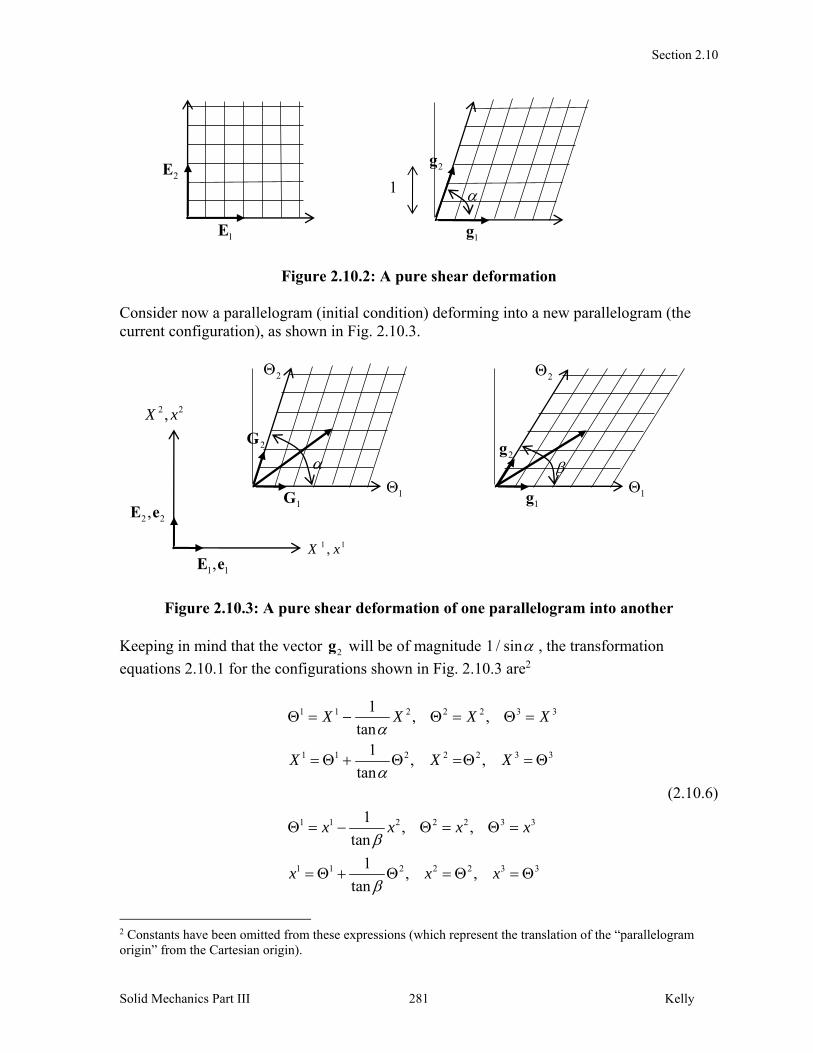
Figure 2.10.2: A pure shear deformation Consider now a parallelogram (initial condition) deforming into a new parallelogram (the current configuration), as shown in Fig. 2.10.3.

Figure 2.10.3: A pure shear deformation of one parallelogram into another Keeping in mind that the vector 2g will be of magnitude 1 / sin , the transformation

equations 2.10.1 for the configurations shown in Fig. 2.10.3 are2

1 1 2 2 2 3 3

1 1 2 2 2 3 3

1 1 2 2 2 3 3

1 1 2 2 2 3 3

1, ,

tan1

, ,tan

1, ,

tan

1, ,

tan

X X X X

X X X

x x x x

x x x

(2.10.6)

2 Constants have been omitted from these expressions (which represent the translation of the “parallelogram origin” from the Cartesian origin).

1E

2E

1g

2g

1

1 1,X x

2 2,X x

1

1 1,E e

2 2,E e1g

2g

2

1

1G

2G

2

Section 2.10

Solid Mechanics Part III Kelly 282

Following on from §1.16, Eqns. 1.16.19, the covariant base vectors are:

1 1 2 1 2 3 3

1 1 2 1 2 3 3

1, , ,

tan

1, , ,

tan

m

i mi

m

i mi

X

X

G E G E G E E G E

g e g e g e e g e

(2.10.7)

and the inverse expressions

1 1 2 1 2 3 3

1 1 2 1 2 3 3

1, ,

tan1

, ,tan

E G E G G E G

e g e g g e g (2.10.8)

Line elements in the configurations can now be expressed as

i i i

i ii

i i ii ii

dd dX d d

dd dx d d

XX E G

xx e g

(2.10.9)

The scale factors, i.e. the magnitudes of the covariant base vectors, are (see Eqns. 1.16.36)

1 1 2 2

1 1 2 2

11,

sin1

1,sin

H H

h h

G G

g g (2.10.10)

The contravariant base vectors are (see Eqn. 1.16.23)

1 2 31 2 2 3

1 2 31 2 2 3

1, , ,

tan

1, , ,

tan

ii

mm

ii

mm

X

X

G E G E E G E G E

g e g e e g e g e

(2.10.11)

and the inverse expressions

Section 2.10

Solid Mechanics Part III Kelly 283

1 2 2 31 2 3

1 2 2 31 2 3

1, ,

tan1

, ,tan

E G G E G E G

e g g e g e g (2.10.12)

The magnitudes of the contravariant base vectors, are

1 1 2 2

1 1 2 2

1, 1

sin1

, 1sin

H H

h h

G G

g g (2.10.13)

The metric coefficients are (see Eqns. 1.16.27)

2

2

2

2

1 1 11 0 0

tan sin tan1 1 1

0 , 1 0tan sin tan

0 0 1 0 0 1

1 1 11 0 0

tan sin tan

1 1 10 , 1 0

tan sin tan

0 0 1 0 0 1

ij i jij i j

ij i jij i j

G G

g g

G G G G

g g g g

(2.10.14)

The transformation determinants are (consistent with zero volume change), from Eqns. 1.16.32-34,

2

2

2

2

1det det 1

det

1det det 1

det

i

ij Gjij

i

ij gjij

XG G J

G

xg g J

g

(2.10.15)

■

Section 2.10

Solid Mechanics Part III Kelly 284

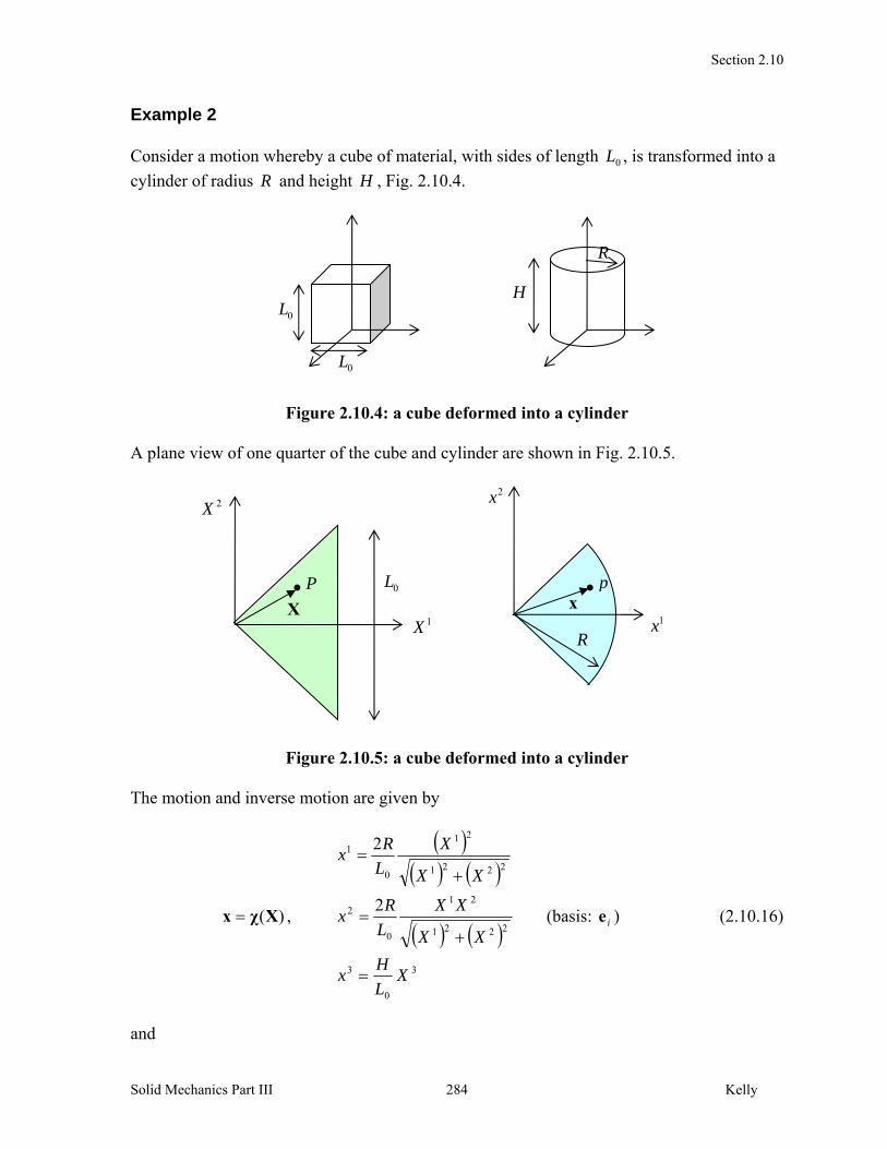
Example 2 Consider a motion whereby a cube of material, with sides of length 0L , is transformed into a

cylinder of radius R and height H , Fig. 2.10.4.

Figure 2.10.4: a cube deformed into a cylinder A plane view of one quarter of the cube and cylinder are shown in Fig. 2.10.5.

Figure 2.10.5: a cube deformed into a cylinder The motion and inverse motion are given by

)(Xχx ,

3

0

3

2221

21

0

2

2221

21

0

1

2

2

XL

Hx

XX

XX

L

Rx

XX

X

L

Rx

(basis: ie ) (2.10.16)

and

0L

R

0LH

1X

2X

1x

2x

0L

R

X x P p

Section 2.10

Solid Mechanics Part III Kelly 285

)(1 xχX ,

303

22211

202

222101

2

2

xH

LX

xxx

x

R

LX

xxR

LX

(basis: iE ) (2.10.17)

Introducing a set of convected coordinates, Fig. 2.10.6, the material and spatial coordinates are

),,( 321 XX ,

303

2102

101

tan2

2

H

LX

R

LX

R

LX

(2.10.18)

and (these are simply cylindrical coordinates)

),,( 321 xx , 33

212

211

sin

cos

x

x

x

(2.10.19)

A typical material particle (denoted by p) is shown in Fig. 2.10.6. Note that the position vectors for p have the same i values, since they represent the same material particle.

Figure 2.10.6: curvilinear coordinate curves

1X

2X

1x

2x

1

2

1

2

R1

42

p p

Section 2.10

Solid Mechanics Part III Kelly 286

■ 2.10.2 The Deformation Gradient With convected curvilinear coordinates, the deformation gradient is

1 2 31 2 3

1 0 0

0 1 0

0 0 1

ii

ji

F g G

g G g G g G

g G

, (2.10.20)

The deformation gradient operates on a material vector (with contravariant components)

iiVV G , resulting in a spatial tensor i

ivv g (with the same components iV v ), for

example,

i j ii j id d d d F X g G G g x (2.10.21)

To emphasise the point, line elements mapped between the configurations have the same coordinates i : a line element 1 2 3

1 2 3d d d G G G gets mapped to

1 2 3 1 2 3 1 2 31 2 3 1 2 3 1 2 3d d d d d d g G g G g G G G G g g g

(2.10.22) This shows also that line elements tangent to the coordinate curves are mapped to new elements tangent to the new coordinate curves; the covariant base vectors iG are a field of

tangent vectors which get mapped to the new field of tangent vectors ig , as illustrated in Fig.

2.10.7.

Figure 2.10.7: Vectors tangent to coordinate curves

dxdX

Section 2.10

Solid Mechanics Part III Kelly 287

The deformation gradient F, the transpose TF and the inverses T1 , FF , map the base

vectors in one configuration onto the base vectors in the other configuration (that the 1F and TF in this equation are indeed the inverses of F and TF follows from 1.16.63):

ii

ii

ii

ii

gGF

GgF

gGF

GgF

T

T

1

ii

ii

ii

ii

GgF

gGF

GgF

gFG

T

T

1

Deformation Gradient (2.10.23)

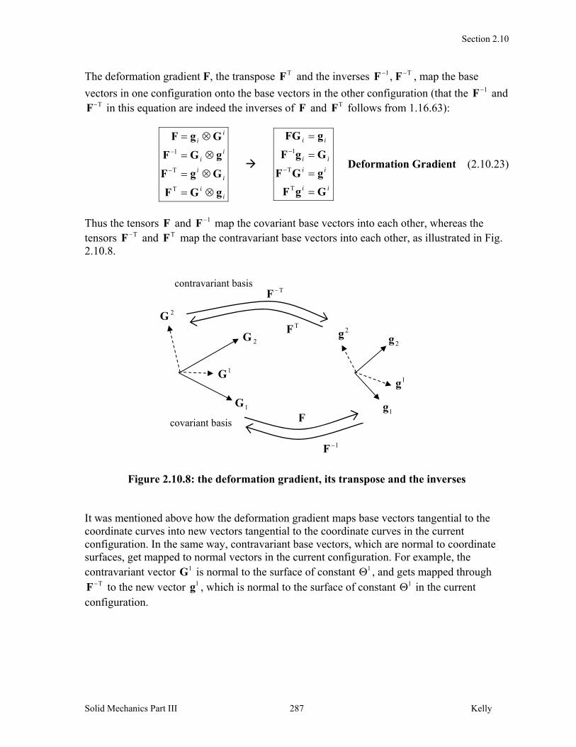
Thus the tensors F and 1F map the covariant base vectors into each other, whereas the tensors TF and TF map the contravariant base vectors into each other, as illustrated in Fig. 2.10.8.

Figure 2.10.8: the deformation gradient, its transpose and the inverses It was mentioned above how the deformation gradient maps base vectors tangential to the coordinate curves into new vectors tangential to the coordinate curves in the current configuration. In the same way, contravariant base vectors, which are normal to coordinate surfaces, get mapped to normal vectors in the current configuration. For example, the contravariant vector 1G is normal to the surface of constant 1 , and gets mapped through

TF to the new vector 1g , which is normal to the surface of constant 1 in the current configuration.

1G

2G

1G

2G

1g

2g

1g

2g

covariant basis

contravariant basis TF

F

1F

TF

Section 2.10

Solid Mechanics Part III Kelly 288

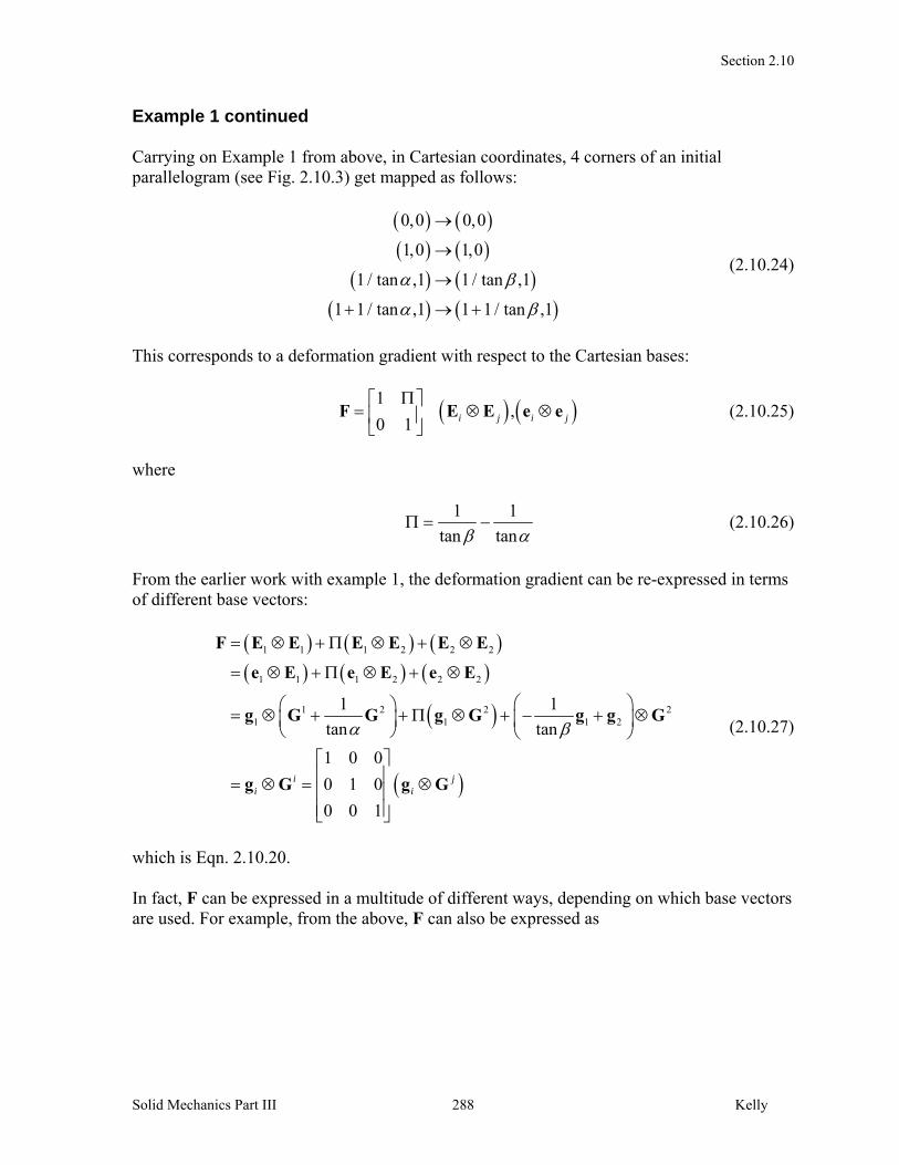
Example 1 continued Carrying on Example 1 from above, in Cartesian coordinates, 4 corners of an initial parallelogram (see Fig. 2.10.3) get mapped as follows:

0,0 0,0

1,0 1,0

1 / tan ,1 1 / tan ,1

1 1 / tan ,1 1 1 / tan ,1

(2.10.24)

This corresponds to a deformation gradient with respect to the Cartesian bases:

1,

0 1 i j i j

F E E e e (2.10.25)

where

1 1

tan tan (2.10.26)

From the earlier work with example 1, the deformation gradient can be re-expressed in terms of different base vectors:

1 1 1 2 2 2

1 1 1 2 2 2

1 2 2 21 1 1 2

1 1

tan tan

1 0 0

0 1 0

0 0 1

i ji i

F E E E E E E

e E e E e E

g G G g G g g G

g G g G

(2.10.27)

which is Eqn. 2.10.20. In fact, F can be expressed in a multitude of different ways, depending on which base vectors are used. For example, from the above, F can also be expressed as

Section 2.10

Solid Mechanics Part III Kelly 289

1 1 1 2 2 2

1 2 1 2 1 2 2 2 21 1 1

tan tan tan

11 0

tan

1 1 10

tan tan tan

0 0 1

i j

F E E E E E E

G G G G G G G G G

G G

(2.10.28) (This can be verified using Eqn. 2.10.30a below.) Components of F The various components of F and its inverses and the transposes, with respect to the different bases, are:

ji

ijj

ijiji

ijjiij

ji

ijj

ijiji

ijjiij

ffff

FFFF

gggggggg

GGGGGGGGF

j

i

i

jjij

iji

ijjiij

ji

i

jjij

iji

ijjiij

ffff

FFFF

gggggggg

GGGGGGGGF

1111

11111

j

i

i

jjij

iji

ijjiij

ji

i

jjij

iji

ijjiij

ffff

FFFF

gggggggg

GGGGGGGGF

TTTT

TTTTT

j

i

i

jjij

iji

ijjiij

ji

i

jjij

iji

ijjiij

ffff

FFFF

gggggggg

GGGGGGGGF

TTTT

TTTTT

(2.10.29)

The components of F with respect to the reference bases ii GG , are

Section 2.10

Solid Mechanics Part III Kelly 290

j

m

m

i

ji

jii

j

kijkj

ij

i

kijkjiij

j

m

i

m

jijiij

x

XF

GF

GF

xXF

gGFGG

gGFGG

gGFGG

gGFGG

(2.10.30)

and similarly for the components with respect to the current bases. Components of the Base Vectors in different Bases The base vectors themselves can be expressed alternately:

mmi

mmi

jim

mj

ji

mmj

ij

mmji

jmmjii

FF

FF

FF

GG

GG

GGGGGGFGg

(2.10.31)

showing that some of the components of the deformation gradient can be viewed also as components of the base vectors. Similarly,

m

m

im

miii ff gggFG 111 (2.10.32)

For the contravariant base vectors, one has

mi

mm

mi

ij

mj

mijm

mj

ij

mj

mi

jm

mjii

FF

FF

FF

GG

GG

GGGGGGGFg

TT

TT

TTT

(2.10.33)

and

mi

mm

miii ff gggFG

TTT (2.10.34)

2.10.3 Reduction to Material and Spatial Coordinates Material Coordinates Suppose that the material coordinates iX with Cartesian basis are used (rather than the convected coordinates with curvilinear basis iG ), Fig. 2.10.9. Then

Section 2.10

Solid Mechanics Part III Kelly 291

jj

ij

j

ii

ji

j

ji

j

i

ijj

ij

j

ii

iji

j

ji

j

iii

x

X

x

X

xx

X

X

X

X

XX

Xeeg

eeg

EEEG

EEEG

,, (2.10.35)

and

XeEgEgGF

xEeEgGgF

grad

Grad

1

jij

ii

ii

i

iji

ji

ii

i

x

X

X

x

(2.10.36)

which are Eqns. 2.2.2, 2.2.4. Thus xGrad is the notation for F and gradX is the notation for

1F , to be used when the material coordinates iX are used to describe the deformation.

Figure 2.10.9: Material coordinates and deformed basis Spatial Coordinates Similarly, when the spatial coordinates ix are to be used as independent variables, then

ijj

ij

j

ii

iji

j

ji

j

i

jj

ij

j

ii

ji

j

ji

j

iii

x

x

x

x

xx

X

x

X

x

XX

xeeeg

eeeg

EEG

EEG

,, (2.10.37)

and

1X

2X

3X

X 1E

2E

1g2g

current configuration

reference configuration

Section 2.10

Solid Mechanics Part III Kelly 292

XeEeGgGF

xEeGeGgF

grad

Grad

1

iji

ji

ii

i

jij

ii

ii

i

x

X

X

x

(2.10.38)

The descriptions are illustrated in Fig. 2.10.10. Note that the base vectors iG , ig are not the

same in each of these cases (curvilinear, material and spatial).

Figure 2.10.10: deformation described using different independent variables

1X

2X

1x

2x

1X

2X

1x

2x

1X

2X

1x

2x

1G2G

1g2g

1E

2E

1g

2g

2G

1G 1e

2e

ii GgF

xEeF Grad

jij

i

X

x

ii gGF 1

XeEF grad1

jij

i

x

X

Section 2.10

Solid Mechanics Part III Kelly 293

2.10.4 Strain Tensors The Cauchy-Green tensors The right Cauchy-Green tensor C and the left Cauchy-Green tensor b are defined by Eqns. 2.2.10, 2.2.13,

ji

ijji

ijj

jii

jiij

jiij

jji

i

ji

ij

jiij

jji

i

jiij

jiij

jji

i

bG

bG

Cg

Cg

gggggGGgFFb

gggggGGgFFb

GGGGGggGFFC

GGGGGggGFFC

11T1

T

1T11

T

(2.10.39)

Thus the covariant components of the right Cauchy-Green tensor are the metric coefficients

ijg . This highlights the importance of C: the ij i jg g g give a clear measure of the

deformation occurring. (It is possible to evaluate other components of C, e.g. ijC , and also its components with respect to the current basis, but only the components ijC with respect to

the reference basis are (normally) used in the analysis.) The Stretch Now, analogous to 2.2.9, 2.2.12,

xxbXX

XXCxx

dddddS

ddddds12

2

(2.10.40)

so that the stretches are, analogous to 2.2.17,

jij

i

jij

i

xdbxdddd

d

d

d

ds

dS

XdCXdddd

d

d

d

dS

ds

ˆˆˆˆ1

ˆˆˆˆ

1112

2

2

2

22

xbxx

xb

x

x

XCXX

XC

X

X

(2.10.41)

The Green-Lagrange and Euler-Almansi Tensors The Green-Lagrange strain tensor E and the Euler-Almansi strain tensor e are defined through 2.2.22, 2.2.24,

Section 2.10

Solid Mechanics Part III Kelly 294

xxexbIx

XXEXICX

dddddSds

dddddSds

122

22

2

1

2

2

1

2 (2.10.42)

The components of E and e can be evaluated through (writing IG , the identity tensor expressed in terms of the base vectors in the reference configuration, and Ig , the identity tensor expressed in terms of the base vectors in the current configuration)

jiij

jiijij

jiij

jiij

jiij

jiijij

jiij

jiij

eGgGg

EGgGg

ggggggggbge

GGGGGGGGGCE

2

1

2

1

2

12

1

2

1

2

1

1

(2.10.43) Note that the components of E and e with respect to their bases are equal, ijij eE (although

this is not true regarding their other components, e.g. ijij eE ). Example 1 continued Carrying on Example 1 from above, consider now an example vector

x

iy

V

V

V E (2.10.44)

The contravariant and covariant components are

1

,tan 1

tan

xx y i

ix y

y

VV V

V VV

V G V G (2.10.45)

The magnitude of the vector can be calculated through (see Eqn. 1.16.52 and 1.16.49)

2 2

2

211 12 22

22 11 12 22

2tan tan

2tan tan

i i

i i

i i

x y

y yi jij x x y y

ij x xi j x x y y

V V

V VG V V V G V V G V G

V VG VV V G V V G V G

E E

G G

G G

V V V

V V

V V

(2.10.46)

Section 2.10

Solid Mechanics Part III Kelly 295

The new vector is obtained from the deformation gradient:

1

0 1

11 0

tantan0 1

i

i

x x y

iy y

yx yx

i

yy

V V V

V V

VV VV

VV

E

G

v F V e

F V g

(2.10.47)

In terms of the contravariant vectors:

1 11

tan tan

x y

j ij

x y

V V

v gV V

v g (2.10.48)

Note that the contravariant components do not change with the deformation, but the covariant components do in general change with the deformation. The magnitudes of the vectors before and after deformation are given by the Cauchy-Green strain tensors, whose coefficients are those of the metric tensors (the first of these is the same as 2.10.46)

1 1 T 1 1

T

i i i i i i

i i i i i i

k i j l i jk ij l ij

k i j l i jk ij l ij

v G v G v v

V g V g V V

g g g g g g

G G G G G G

V V F v F v vF F v vb v g g g g

v v F V F V V F F V VCV G G G G

(2.10.49)

From this, the magnitude of the vector after deformation is

2 2 2i jij x y y x yg V V V V V V V v v (2.10.50)

2.10.5 Intermediate Configurations Stretch and Rotation Tensors The polar decompositions vRRUF have been described in §2.2.5. The decompositions are illustrated in Fig. 2.10.11. In the material decomposition, the material is first stretched by U and then rotated by R. Let the base vectors in the associated intermediate configuration be ig . Similarly, in the spatial decomposition, the material is first rotated by R and then

stretched by v. Let the base vectors in the associated intermediate configuration in this case be iG . Then, analogous to Eqn. 2.10.23, {▲Problem 1}

Section 2.10

Solid Mechanics Part III Kelly 296

ii

ii

ii

ii

gGU

GgU

gGU

GgU

ˆ

ˆ

ˆ

ˆ

T

T

1

ii

ii

ii

ii

GgU

gGU

GgU

gUG

ˆ

ˆ

ˆ

ˆ

T

T

1

(2.10.51)

ii

ii

ii

ii

gGv

Ggv

gGv

Ggv

ˆ

ˆ

ˆ

ˆ

T

T

1

ii

ii

ii

ii

Ggv

gGv

Ggv

gGv

ˆ

ˆ

ˆ

ˆ

T

T

1

(2.10.52)

Figure 2.10.11: the material and spatial polar decompositions Note that U and v symmetric, TUU , Tvv , so

iii

i

iii

i

GggGU

gGGgU

ˆˆ

ˆˆ1

ii

ii

iiii

gGUGgU

GgUgUG

ˆ,ˆ

ˆ,ˆ11

(2.10.53)

iii

i

iii

i

GggGv

gGGgv

ˆˆ

ˆˆ

1

ii

ii

iiii

gGvGgv

GvggGv

ˆ,ˆ

ˆ,ˆ

11 (2.10.54)

Similarly, for the rotation tensor, with R orthogonal, T1 RR ,

iii

i

iii

i

GGGGR

GGGGR

ˆˆ

ˆˆ

T

iiii

iiii

GGRGGR

GRGGRG

ˆ,ˆ

ˆ,ˆ

TT (2.10.55)

iii

i

iii

i

ggggR

ggggR

ˆˆ

ˆˆT

ii

ii

iiii

ggRggR

ggRggR

ˆ,ˆ

ˆ,ˆTT

(2.10.56)

iG

igU R

ig

iGR v

Section 2.10

Solid Mechanics Part III Kelly 297

The above relations can be checked using Eqns. 2.10.23 and RUF , vRF , 11 RFv , etc. Various relations between the base vectors can be derived, for example,

ji

ji

ji

ji

jiji

jijijiji

gGgG

gGgG

gGgG

gGgRRGgRRGgG

ˆˆ

ˆˆ

ˆˆ

ˆˆˆˆ T

(2.10.57)

Deformation Gradient Relationship between Bases The various base vectors are related above through the stretch and rotation tensors. The intermediate bases are related directly through the deformation gradient. For example, from 2.10.53a, 2.10.55b,

iiii GFGURUGg ˆˆˆ TT (2.10.58)

In the same way,

ii

ii

ii

ii

gFG

gFG

GFg

GFg

ˆˆ

ˆˆ

ˆˆ

ˆˆ

T

1

T

(2.10.59)

Tensor Components The stretch and rotation tensors can be decomposed along any of the bases. For U the most natural bases would be iG and iG , for example,

ji

ji

jij

iji

ji

jii

jj

iij

mjimjiij

jiij

jijiijji

ij

UU

UU

GUU

UU

GgUGGGGU

gGUGGGGU

gGUGGGGU

gGUGGGGU

ˆ,

ˆ,

ˆ,

ˆ,

(2.10.60)

with j

ij

iij

ij

jiijjiij UUUUUUUU

,,, . One also has

Section 2.10

Solid Mechanics Part III Kelly 298

ji

ji

jij

iji

ji

jii

jj

iij

mjimjiij

jiij

jijiijji

ij

vv

vv

Gvv

vv

GgGvGGGv

gGGvGGGv

gGGvGGGv

gGGvGGGv

ˆˆˆ,ˆˆ

ˆˆˆ,ˆˆ

ˆˆˆˆ,ˆˆ

ˆˆˆ,ˆˆ

(2.10.61)

with similar symmetry. Also,

j

ij

i

j

ijij

i

ji

jii

jj

i

i

j

jm

imjiij

ji

ij

jijiijji

ij

UU

UU

gUU

UU

gGgUgggU

GggUgggU

gGgUgggU

gGgUgggU

ˆˆˆ,ˆˆ

ˆˆˆ,ˆˆ

ˆˆˆˆ,ˆˆ

ˆˆˆ,ˆˆ

1111

1111

1111

1111

(2.10.62)

and

j

ij

i

j

ijij

i

ji

jii

jj

i

i

j

im

mjjiij

ji

ij

jijiijji

ij

vv

vv

gvv

vv

gGgvgggv

Gggvgggv

gGgvgggv

gGgvgggv

ˆ,

ˆ,

ˆ,

ˆ,

1111

1111

1111

1111

(2.10.63)

with similar symmetry. Note that, comparing 2.10.60a, 2.10.61a, 2.10.62a, 2.10.63a and using 2.10.57,

ijijijij

jiij

jiij

jiij

jiij

vvUU

v

U

v

U

11

11

11 ˆˆ

ˆˆ

ggv

ggU

GGv

GGU

(2.10.64)

Now note that rotations preserve vectors lengths and, in particular, preserve the metric, i.e.,

jiijjiij

jiijjiij

gg

GG

gggg

GGGG

ˆˆˆ

ˆˆˆ

(2.10.65)

Thus, again using 2.10.57, and 2.10.60-2.10.63, the contravariant components of the above

tensors are also equal, ijijijij vvUU 11 .

Section 2.10

Solid Mechanics Part III Kelly 299

As mentioned, the tensors can be decomposed along other bases, for example,

jijiijji

ij vv gGvggggv ˆ, (2.10.66)

2.10.6 Eigenvectors and Eigenvalues Analogous to §2.2.5, the eigenvalues of C are determined from the eigenvalue problem

0det IC C (2.10.67)

leading to the characteristic equation 1.11.5

0IIIIII 23 CCCCCC (2.10.68)

with principal scalar invariants 1.11.6-7

321321

1332212122

21

321

detIII

)tr()(trII

trI

CCCC

CCCCCCC

CCCC

C

CC

C

kjiijk

ji

ij

jj

ii

ii

CCC

CCCC

A

(2.10.69)

The eigenvectors are the principal material directions iN , with

0NIC iiˆ (2.10.70)

The spectral decomposition is then

3

1

2 ˆˆi

iii NNC (2.10.71)

where 2

ii C and the i are the stretches. The remaining spectral decompositions in

2.2.37 hold also. Note also that the rotation tensor in terms of principal directions is (see 2.2.35)

iii

i NnNnR ˆˆˆˆ (2.10.72)

where in are the spatial principal directions.

Section 2.10

Solid Mechanics Part III Kelly 300

2.10.7 Displacement and Displacement Gradients Consider the displacement u of a material particle. This can be written in terms of covariant components iU and iu :

i

ii

i uU gGXxu . (2.10.73)

The covariant derivative of u can be expressed as

m

imm

imiuU gG

u

(2.10.74)

The single line refers to covariant differentiation with respect to the undeformed basis, i.e. the Christoffel symbols to use are functions of the ijG . The double line refers to covariant

differentiation with respect to the deformed basis, i.e. the Christoffel symbols to use are functions of the ijg .

Alternatively, the covariant derivative can be expressed as

iiiiiGg

Xxu

(2.10.75)

and so

m

m

imi

mmi

m

imii

mmimi

mmi

m

imii

fuu

FUU

ggggG

GGGGg

1

(2.10.76)

The last equalities following from 2.10.31-32. The components of the Green-Lagrange and Euler-Almansi strain tensors 2.10.43 can be written in terms of displacements using relations 2.10.76 {▲Problem 2}:

j

n

inijjiijijij

j

n

inijjiijijij

uuuuGge

UUUUGgE

2

1

2

12

1

2

1

(2.10.77)

In terms of spatial coordinates, j

ijiii

ii XxX egEG /,, , jiji XUU / , the

components of the Euler-Lagrange strain tensor are

Section 2.10

Solid Mechanics Part III Kelly 301

jk

ik

i

j

ji

ijmnj

n

i

m

ijijij X

U

X

U

X

U

X

U

X

x

X

xGgE

2

1

2

1

2

1 (2.10.78)

which is 2.2.46. 2.10.8 The Deformation of Area and Volume Elements Differential Volume Element Consider a differential volume element formed by the elements i

id G in the undeformed

configuration, Eqn. 1.16.43:

321 dddGdV (2.10.79) where, Eqn. 1.16.31,1.16.34,

jiijij GGG GG ,det (2.10.80)

The same volume element in the deformed configuration is determined by the elements

iid g :

321 dddgdv (2.10.81)

where

jiijij ggg gg ,det (2.8.82)

From 1.16.53 et seq., 2.10.11,

F

GGG

ggg

det

321

321

321

G

GFFF

FFF

g

ijkkji

kjikji

(2.10.83)

where ijk is the Cartesian permutation symbol, and so the Jacobian determinant is (see

2.2.53)

FdetG

g

dV

dvJ (2.10.84)

Section 2.10

Solid Mechanics Part III Kelly 302

and Fdet is the determinant of the matrix with components i

jF .

Differential Area Element Consider a differential surface (parallelogram) element in the undeformed configuration,

bounded by two vector elements )1(Xd and )2(Xd , and with unit normal N . Then the vector normal to the surface element and with magnitude equal to the area of the surface is, using 1.16.54, given by

kjiijkj

ji

i ddedddddS GGGXXN G )2()1()2()1()2()1(ˆ (2.10.85)

where G

ijke is the permutation symbol associated with the basis iG , i.e.

Ge ijkkjiijkijk GGGG . (2.10.86)

Using kk gFG T , one has

kjiijk ddGdS gFN T)2()1(ˆ (2.10.87)

Similarly, the surface vector in the deformed configuration with unit normal n is

kjiijkj

ji

i ddeddddds gggxxn g )2()1()2()1()2()1(ˆ (2.10.88)

where g

ijke is the permutation symbol associated with the basis ig , i.e.

ge ijkkjiijkijk gggg . (2.10.89)

Comparing the two expressions for the areas in the undeformed and deformed configurations, 2.10.87-88, one finds that

dSdSG

gds NFFNFn TT detˆ (2.10.90)

which is Nanson’s relation, Eqn. 2.2.59. This is consistent with was said earlier in relation to Fig. 2.10.8 and the contravariant bases: TF maps vectors normal to the coordinate curves in the initial configuration into corresponding vectors normal to the coordinate curves in the current configuration.

Section 2.10

Solid Mechanics Part III Kelly 303

2.10.9 Problems 1. Derive the relations 2.10.51. 2. Use relations 2.10.76, with jiijg gg and jiijG GG , to derive 2.10.77

j

n

inijjiijijij

j

n

inijjiijijij

uuuuGge

UUUUGgE

2

1

2

12

1

2

1