The Department of Engineering Science

The University of Auckland

Welcome to ENGGEN 131

Engineering Computation and

Software Development

Chapter 10

Linear Equations

and

Linear Algebra

STUDY SUPPORT FOR

PART I STUDENTS• Current Part II & III students employed as Part I Mentors to provide

help/tutoring for all Part I students across all Part I courses

• We are there to help you with your– Weekly tutorial problems– Assignments (by working through similar model questions)– Preparation for tests or exams

• WON’T JUST GIVE YOU THE ANSWER

• Service for everyone – NOT just those who are struggling (Let us help you turn a B+ into an A, as well as a fail into a pass)

• Happy to provide general advice (on learning strategies, coping with workload, choosing your specialisation)

• Happy to provide one-on-one or group tutoring (so if shy about coming on your own, bring a friend!)

Part I Assistance CentreSummer School

Mondays, Wednesdays and Fridays

11am –3pm

(excluding public holidays) Leech Study Area

PART I ASSISTANCE CENTRE Leech

Study Area

• Summer School Opening Hours

Mondays, Wednesdays and Fridays11am-3pm

Commencing Monday 9th January –Friday 17th February (excluding public holidays).

• FREE support is provided to help you

– Prepare for tests or exams– Go through weekly tutorial problems– Prepare for assignments by working through

similar model questions

Note about Chapter 9

• Chapter 9 on Files is NOT part of the examinable material for ENGGEN131AC.

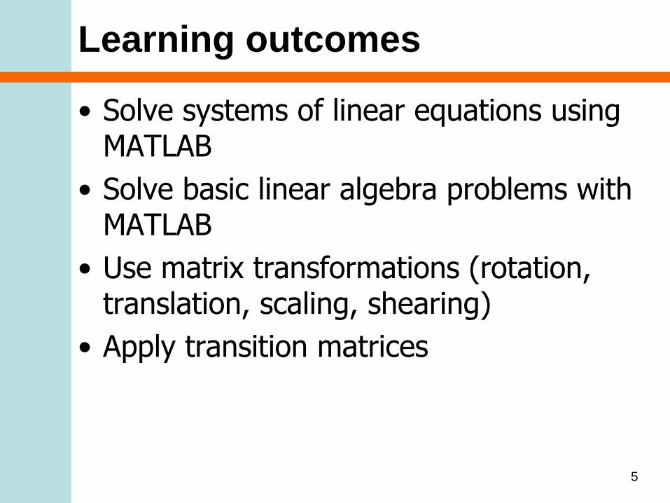
Learning outcomes

• Solve systems of linear equations using MATLAB

• Solve basic linear algebra problems with MATLAB

• Use matrix transformations (rotation, translation, scaling, shearing)

• Apply transition matrices

5

Solving systems of linear equations

6

7

To solve this equation in MATLAB we simply type the following:

A = [1 2 3; 2 5 3; 1 0 8];

b = [1; 6; -6];

x = A \ b

The left division method performs the equivalent to Gaussian

elimination

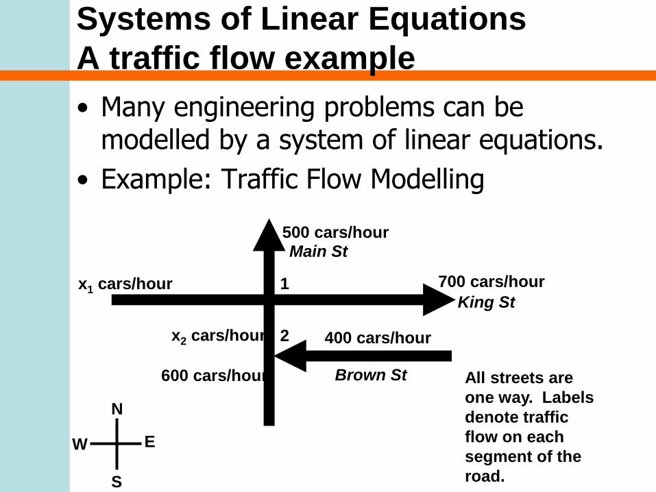
Systems of Linear Equations

A traffic flow example

• Many engineering problems can be modelled by a system of linear equations.

• Example: Traffic Flow Modelling

500 cars/hour

x1 cars/hour 700 cars/hour

400 cars/hourx2 cars/hour

600 cars/hour All streets are

one way. Labels

denote traffic

flow on each

segment of the

road.

1

2

Brown St

King St

Main St

S

N

EW

5 Steps for Problem Solving

1. State the problem clearly

2. Describe the input and output information

3. Work the problem by hand (or with a calculator) for a simple set of data

4. Develop a solution and convert it to a computer program

5. Test the solution with a variety of data

1. State the Problem Clearly

Determine x1 and x2 using the known traffic flows of 400, 500, 600 and 700 cars/hour on segments of Main St, King St and Brown St (which are one way streets).

2. Describe the input and output

information

Input:

– Main St (north of intersection 1), 500 cars/hour

- King St (west of intersection 1), 700 cars/hour

- Brown St, 400 cars/hour

- Main St (south of intersection 2), 600 cars/ hour

Output:

- x1 cars per hour travelling on King St (east of intersection 1)

- x2 cars per hour travelling on Main St (between intersection 1 and intersection 2)

3. Work the Problem by Hand

• Balance the flow of cars into and out of each intersection.

• Intersection 1

• Intersection 2

clearly x2 is equal to 1000 cars/hour, so

4006002 x

70050021 xx

200

12001000

1

1

x

x

4. Develop a Solution and Convert

it to a Computer Program

• The two equations we need to solve can be expressed as

• To solve this problem in Matlab we can use the “left division” operator

1000

1200

10

11

2

1

x

x

A = [1, 1; 0, 1;]

b = [1200; 1000;]

x = A\b

Solving basic linear algebra problems

(not examined in Summer School)

• Find the angle between two vectors

• Find the projection of one vector onto another

• Find the area of a triangle defined by two vectors

• Find the equation of a plane containing three points

14

Matrix Transformations

• A point (or points) can be transformed by using a square matrix. It is possible to create matrices representing stretches, enlargements, reflections and rotation.

• To transform a point we perform a matrix multiplication with the transformation matrix and the point.

15

16

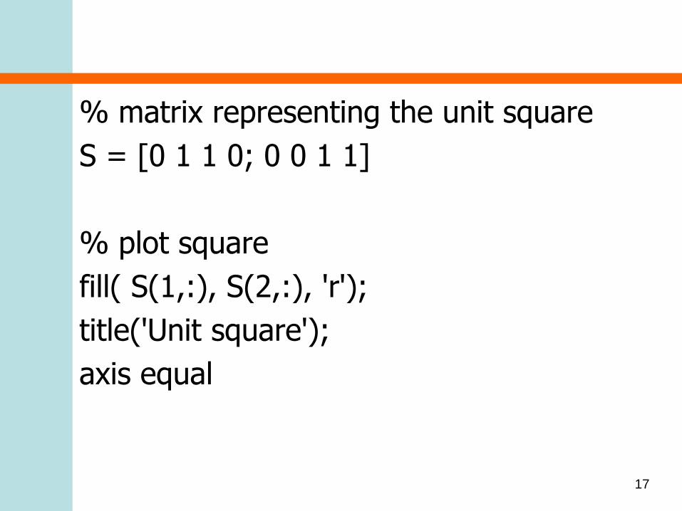
% matrix representing the unit square

S = [0 1 1 0; 0 0 1 1]

% plot square

fill( S(1,:), S(2,:), 'r');

title('Unit square');

axis equal

17

18

0 0.2 0.4 0.6 0.8 10

0.1

0.2

0.3

0.4

0.5

0.6

0.7

0.8

0.9

1Unit square

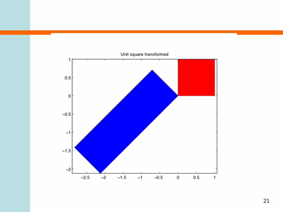
% matrix to stretch x axis by a factor of 3

X = [3 0; 0 1]

% matrix to reflect in y axis

Y = [-1 0; 0 1]

% matrix to rotate by pi/4 radians (45 degrees)

R = [cos(pi/4) -sin(pi/4); sin(pi/4) cos(pi/4)]

19

% perform transformations

T = R * Y * X *S

% plot transformed square

hold on

fill( T(1,:), T(2,:), 'b');

20

21

Transition Matrices

• (not examined in Summer School)

22

Chapter 10 Summary

How would you solve the following system of equations using MATLAB?

2x1 + x3 = 5

x1 + 4x2 + 3x3 = 0

x2 + 5x3 - 9 = 0

Option A A=[2,1,5;1,4,3,0;1,5,-9,0]; b=[5;0;0]; x=A\b

Option B A=[2,1,5;1,4,3,0;1,5,-9,0]; b=[5;0;9]; x=A\b

Option C A=[2,0,1;1,4,3;0,1,5]; b=[5;0;9]; x=A/b

Option D A=[2,0,1;1,4,3;0,1,5]; b=[5;0;9]; x=A\b

What effect will the following transformation matrix produce?

[-1,0;0,-1]

Option A Shift to the left.

Option B Rotation by 90 degrees clockwise.

Option C Reflection in both x and y planes

Option D Scaling by -1 in the y direction24

The Department of Engineering Science

The University of Auckland

Welcome to ENGGEN 131

Engineering Computation and

Software Development

Chapter 11

Differential Equations

and

“Function” Functions

Learning outcomes

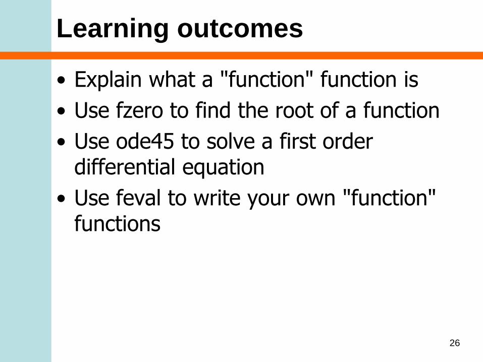
• Explain what a "function" function is

• Use fzero to find the root of a function

• Use ode45 to solve a first order differential equation

• Use feval to write your own "function" functions

26

What is a "function" function?

• Where a function needs to have access to another specified function in order to perform its task.

• This name of this function is provided as an input argument to the first function.

27

Finding roots with fzero

• The fzero function allows us to find xvalues for any function f(x), such that f(x)=0 . These x values are called roots.

• Consider the problem of solving the equation: x2 – x – 12 = 0

• This can be done by hand but it is also easy to solve using MATLAB.

28

function px = MyPolynomial(x)

px = x.^2 - x - 12;

return

• For example to look for roots near x=5

root = fzero(@MyPolynomial, 5)

• This will produce

root =

429

• To find the other root we need to start looking from a different value:

root = fzero(@MyPolynomial, -5)

• This will produce the following output:

root =

-3

• The @ symbol indicates the name of the function for fzero to evaluate 30

Solving ODEs in MATLAB

• dy/dt = f(t,y)

• the derivative can be written as some function of the independent variable and dependent variable.

31

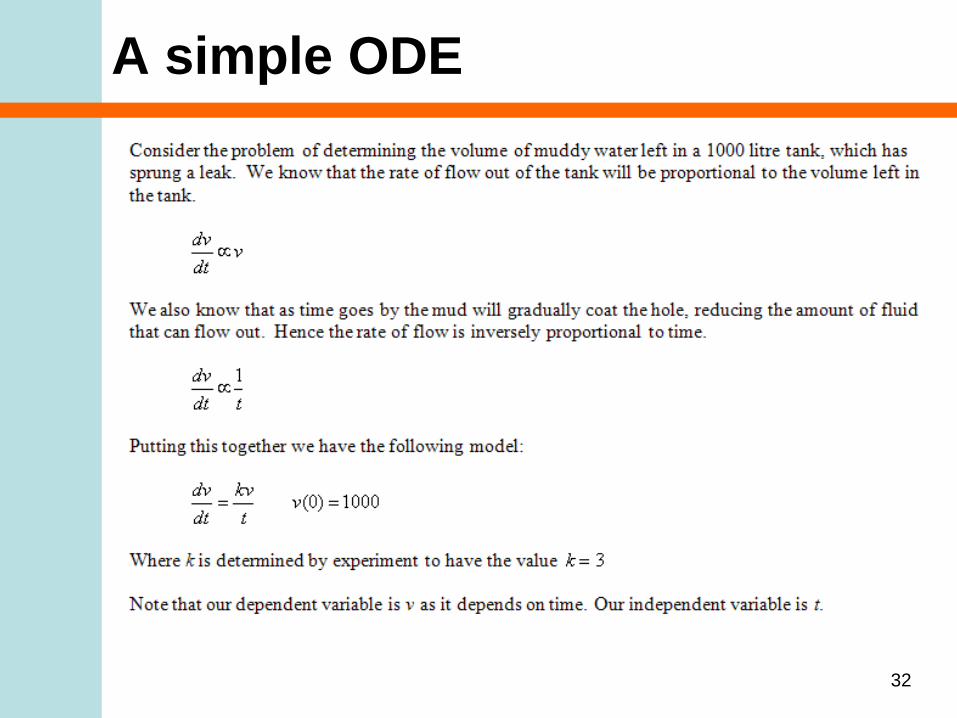
A simple ODE

32

ODE45

The MATLAB solver functions need:

1. A MATLAB function that calculates the derivative for any given values of the independent and dependent variables

2. time span array containing two values (a start time and finish time)

3. An initial value

It will produce two outputs:

1. An array of time values (the independent variable)

2. An array of corresponding solution values (the dependent variable)

33

Create our function definition

function dvdt = MuddyTankFlowRate(t,v)

% calculate the flow rate out of a muddy tank of water

% inputs: v the volume of water

% t the time since the start of the flow

% output: dvdt the flow rate

k = 3;

dvdt = k * v / t;

return

34

Set initial conditions. Call ODE45

% Script to solve the volume of fluid left in a muddy tank

% that contains a hole

% set up a time span of 10 minutes (t is measured in seconds)

timeSpan = [0, 600]

% the initial volume at time t=0 is 1000 litres

vInit = 1000

% solve our ODE

[t,v] = ode45(@MuddyTankFlowRate, timeSpan, vInit);35

Output of ODE45

t

1

1.01674590954340

1.03349181908679

.........

6.83913766802859

6.91956883401430

7

36

v1000951.398686926528905.896867659521863.251189185083.........3.126755174227683.018984210180012.91610943086821

Use results

% plot result

plot(t,v)

title('Plot of fluid level in tank of muddy water')

xlabel('time (seconds)');

ylabel('volume (litres)')

37

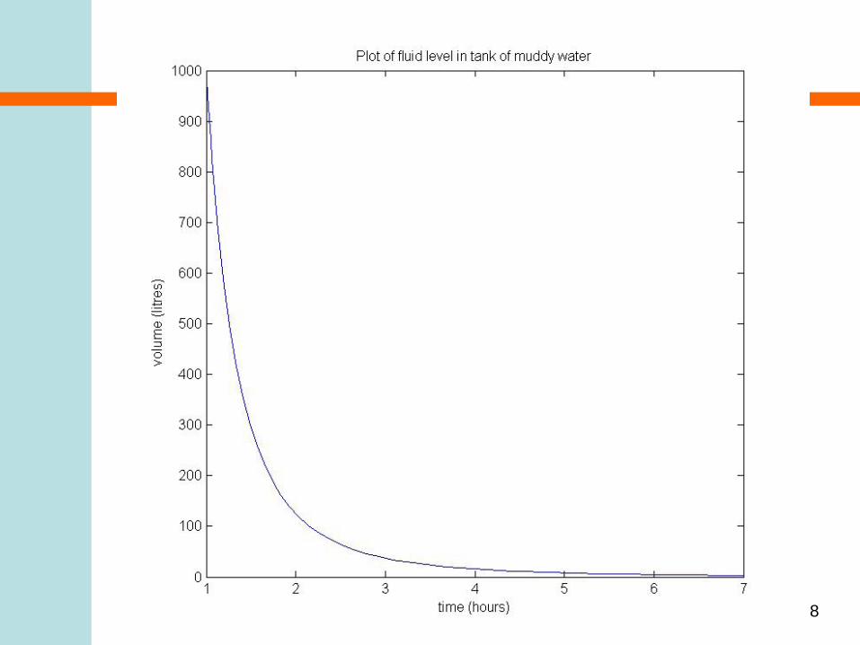
38

feval

• We can write our own "function" functions

function px = MyPolynomial(x)

px = x.^2 - x - 12;

return

Call passing required arguments

p = feval(@MyPolynomial,2)

39

Function name stored as a variable

% create a variable to contain the address of our function

myFunctionAddress = @MyPolynomial;

p = feval(myFunctionAddress,2)

40

Chapter 11 Summary

Which statement about ODE45 is FALSE?

Option A It requires a range of time values.

Option B It requires a set of initial conditions.

Option C It requires a definition of the differential equations.

Option D It plots each solved value against time.

Is the code:

ChosenFunction=@ImperialToMetric;

m=feval(ChosenFunction,6,2);the same as the code:

m=ImperialToMetric(6,2);

Option A Yes

Option B No

42

Test on Friday

Friday’s lab session is designated for Lab 6 and the MATLAB test.

The test will start at 4:30pm.

43