3188 IEEE TRANSACTIONS ON ANTENNAS AND … · 3188 IEEE TRANSACTIONS ON ANTENNAS AND PROPAGATION,...

3188 IEEE TRANSACTIONS ON ANTENNAS AND PROPAGATION, VOL. 56, NO. 10, OCTOBER 2008

On Electromagnetics and Information TheoryMarco Donald Migliore, Member, IEEE

Abstract—Some connections are described between electromag-netic theory and information theory, identifying some unavoidablelimitations imposed by the laws of electromagnetism to communi-cation systems. Starting from this result, the role of the degrees offreedom of the field in radiating systems is investigated. Differentclasses of antennas use the available degrees of freedom in differentways. In particular, a multiple-input multiple-output antenna is aradiating system conveying statistically independent informationon more than one degree of freedom of the field. Applications ofthe theory to antenna synthesis and antenna characterization incomplex environments are shown.

Index Terms—Antenna measurement, antenna synthesis, an-tennas, channel capacity, multiple-input multiple-output (MIMO)systems, number of degrees of freedom (NDF).

I. INTRODUCTION

S OON AFTER the publication of Claude Shannon’s fun-damental papers on Information theory, a great deal of

research has been devoted to the application of this theoryto physics [1]. This effort has shown interesting connectionsbetween information theory and a large number of differentfields of physics, including thermodynamics, optics, computa-tion, quantum theory and astrophysics. Instead, the connectionbetween electromagnetic theory and information theory hasbeen object of little research in the past, and only recentlythere is an interest toward the connections between these twotheories [2]–[10]. As a consequence, a clear understanding ofthe unavoidable limitations imposed by the laws of electro-magnetism to our ability to communicate is not available yet.This understanding is fundamental since it enables the Shannon“mathematical theory of communication” to be connected tothe real world.

This paper represents a further contribution toward the un-derstanding of the relationship between the information theoryand the electromagnetic theory, and how to use this relationshipfor practical applications. A key point to reach this goal is theuse of Kolmogorov approach [11] besides the classic Shannonprobabilistic approach [12] to introduce two important informa-tional quantities: the amount of information associated to a spa-tial distribution of the electromagnetic field and the amount ofinformation reliably conveyed by the electromagnetic field. Theadvantage of the Kolmogorov approach in our context is that it isan operatorial-based communication theory, and consequently itnaturally matches the classic electromagnetic theory approach.In particular, a strong connection between the “degree of com-plexity” of a set of functions, e.g., the infimum of the number

Manuscript received June 25, 2007; revised February 15, 2008. Current ver-sion published October 3, 2008.

The author is with the Microwave Laboratory of the University of Cassino,Via Di Biasio 43, 03043 Cassino, Italy (e-mail: [email protected]).

Digital Object Identifier 10.1109/TAP.2008.929444

of functions required to represent the set of functions within agiven accuracy, and the “amount of information” that the set offunctions can convey in presence of noise is shown.

This result, that regards completely general communicationsystems, when applied to antennas naturally suggests a com-pletely new point of view, in which antennas are characterizedfrom their ability to transmit information. A straightforwardconsequence is a novel unified approach to antennas that in-cludes classic antennas, adaptive antennas and multiple-inputmultiple-output (MIMO) antennas.

The starting point to reach this goal is to consider the phys-ical system consisting of the field radiated by an electromagneticsource (usually the antenna, but more generally a complex en-semble of antennas and scattering objects) and observed on agiven manifold. Like any physical system, the field can be rep-resented by means of a number of state variables. The minimumnumber of state variables allowing to represent the field on theobservation manifold within a desired accuracy is the numberof degrees of freedom (NDF) of the field [13].

A key result of this paper is that an electromagnetic sourcecan use the available NDF of the field basically in two differentways, to approximate the field to a desired field distribution, orto send or receive statistically independent information. Classicantennas use the NDF in the first way, while MIMO antennasuse them in the latter way.

The “information based” approach to antennas proposed inthis paper is not only conceptually interesting, but has prac-tical applications. Examples regarding antenna synthesis andantenna characterization in complex environments are shown inthe paper.

II. SOME LIMITATIONS IN THE AMOUNT OF INFORMATION

ASSOCIATED TO THE ELECTROMAGNETIC FIELD

A. The Amount of Information Associated to the SpatialDistribution of the Electromagnetic Field at an -Level ofUncertainty

As preliminary step, let us recall some analytical propertiesof the field radiated by an harmonic source having finite spatialextension.

In the following the time dependence ( beingthe frequency of the signal) will be understood and dropped.

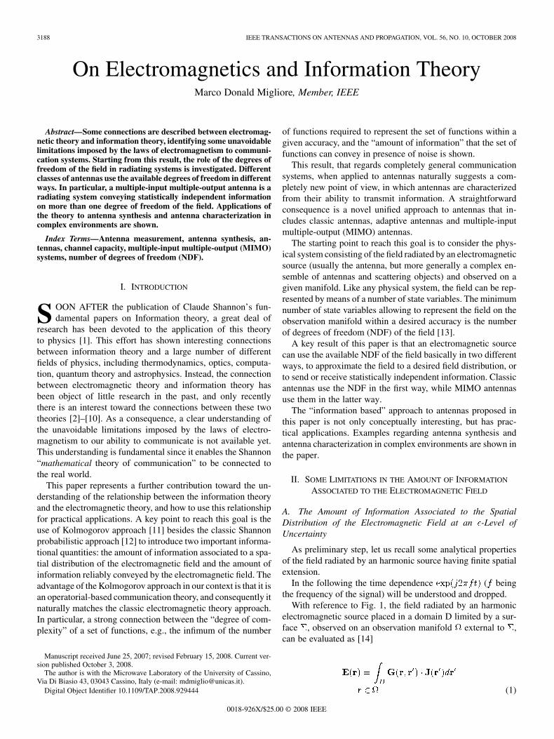
With reference to Fig. 1, the field radiated by an harmonicelectromagnetic source placed in a domain D limited by a sur-face , observed on an observation manifold external to ,can be evaluated as [14]

(1)

0018-926X/$25.00 © 2008 IEEE

MIGLIORE: ON ELECTROMAGNETICS AND INFORMATION THEORY 3189

Fig. 1. Geometry of the problem; D is the domain containing the sources, isthe observation manifold.

Fig. 2. Radiating system model; A models the radiation operator;M modelsthe measurement operator, u the uncertainty level affecting the measured dataz.

where is the source current density in the space, is thedyadic Green’s function [14], and the dot denotes the matrix-vector product.

We can discuss the above problem in a more abstract way,using classical tools of functional analysis, in which the function

is an element in a metric space , and the function isan element in a metric space . In the following we restrictour attention to Hilbert space equipped with the usual normon . In this space many concepts can be explained using asimple geometrical approach, helping to clarify some otherwisequite abstract concepts. The main results showed in this Sectionregarding approximation and information content are valid inmuch more general metric spaces. The interested reader can findmore details in [15]–[18].

In Fig. 2 an abstract model of the radiating system is drawn,wherein is the integral operator in (1), while therole of the measurement operator will be discussed in thefollowing.

Regarding the domain of the operator , we suppose thatis a bounded set, e.g., . Geometrically, the set of thesource currents is contained in a sphere having finite radius .The square radius of the sphere represents the energy (radiatedand stored) of the source.

Since the observation manifold is outside the domain con-taining the sources, the kernel of the radiation operator is ana-lytic. Consequently is a compact (or completely continuous)operator [14], and can be expanded using the Hilbert-Schmidtdecomposition (or singular value decomposition) obtaining

(2)

wherein , , are the left singular functions, the right sin-gular functions and the singular values of the operator respec-tively, and denotes the inner product in . For more

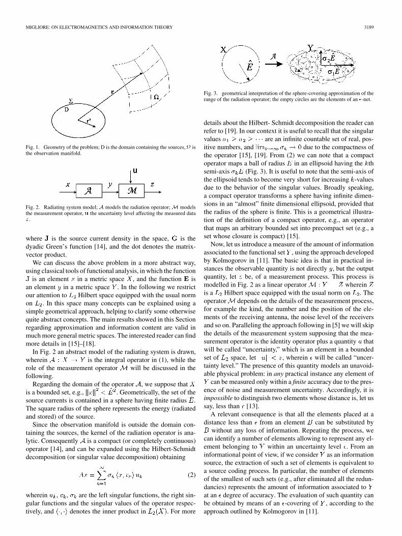
Fig. 3. geometrical interpretation of the sphere-covering approximation of therange of the radiation operator; the empty circles are the elements of an �-net.

details about the Hilbert- Schmidt decomposition the reader canrefer to [19]. In our context it is useful to recall that the singularvalues are an infinite countable set of real, pos-itive numbers, and due to the compactness ofthe operator [15], [19]. From (2) we can note that a compactoperator maps a ball of radius in an ellipsoid having the thsemi-axis (Fig. 3). It is useful to note that the semi-axis ofthe ellipsoid tends to become very short for increasing -valuesdue to the behavior of the singular values. Broadly speaking,a compact operator transforms a sphere having infinite dimen-sions in an “almost” finite dimensional ellipsoid, provided thatthe radius of the sphere is finite. This is a geometrical illustra-tion of the definition of a compact operator, e.g., an operatorthat maps an arbitrary bounded set into precompact set (e.g., aset whose closure is compact) [15].

Now, let us introduce a measure of the amount of informationassociated to the functional set , using the approach developedby Kolmogorov in [11]. The basic idea is that in practical in-stances the observable quantity is not directly , but the outputquantity, let be, of a measurement process. This process ismodelled in Fig. 2 as a linear operator whereinis a Hilbert space equipped with the usual norm on . Theoperator depends on the details of the measurement process,for example the kind, the number and the position of the ele-ments of the receiving antenna, the noise level of the receiversand so on. Paralleling the approach following in [5] we will skipthe details of the measurement system supposing that the mea-surement operator is the identity operator plus a quantity thatwill be called “uncertainty,” which is an element in a boundedset of space, let , wherein will be called “uncer-tainty level.” The presence of this quantity models an unavoid-able physical problem: in any practical instance any element of

can be measured only within a finite accuracy due to the pres-ence of noise and measurement uncertainty. Accordingly, it isimpossible to distinguish two elements whose distance is, let ussay, less than [13].

A relevant consequence is that all the elements placed at adistance less than from an element can be substituted by

without any loss of information. Repeating the process, wecan identify a number of elements allowing to represent any el-ement belonging to within an uncertainty level . From aninformational point of view, if we consider as an informationsource, the extraction of such a set of elements is equivalent toa source coding process. In particular, the number of elementsof the smallest of such sets (e.g., after eliminated all the redun-dancies) represents the amount of information associated toat an degree of accuracy. The evaluation of such quantity canbe obtained by means of an -covering of , according to theapproach outlined by Kolmogorov in [11].


We recall that a system of sets is called an -cov-ering of the set if the diameter of an arbitrarydoes not exceed and [11], [14]. A set

is called an -net for the set if every element of the setis at a distance not exceeding from some element of [11].With reference to Fig. 3, we can image an -covering of as afamily of open balls with centres in and radius whose unionincludes . The minimal number of -balls required to cover ,expressed in bits, is called the Kolmogorov -entropy (calledalso “metric entropy,” in contradistinction to the Shannon prob-abilistic entropy) [11], [16]. Any -net having a number of ele-ments equal to the Kolmogorov -entropy allows to approximate

at level using the smallest subset, e.g., in the “most econom-ical” way, and will be called an optimal -net. With reference toFig. 3, if we suppose that the -covering is minimal, the set ofelements on which the balls are centred gives an optimal -net.For a more rigorous discussion regarding the relationship be-tween -covering and -net in metric spaces the reader can referto [11] and [16].

Since is precompact the -entropy turns out to be finite forany [11], [13]. In our specific context, it means that anypattern belonging to can be approximated by a pattern be-longing to a finite ( -entropy) number of patterns for any accu-racy .

Note that any optimal -net represents a minimum lengthcodebook able to represent any element of Y within a level ofaccuracy . Accordingly, the -entropy is the amount of infor-mation, measured in bits, associated to at an degree of ac-curacy [13].

It is interesting to note that an increasing of (e.g., )increases the length of the semi-axes of the ellipsoid in Fig. 3.Consequently, also semi-axes associated to small singularvalues give a not negligible contribution, increasing the volumeof the ellipsoid, and consequently the -entropy. In particular,if we leave the domain of unbounded we can obtain anarbitrarily large -entropy. This happens, for example, im-posing a constraint only on the total radiated energy (associatedto the radiated power), allowing an arbitrarily high level ofreactive energy. Accordingly, superdirective sources [20] areable to give, at least theoretically, fields whose -entropy canbe arbitrarily high.

Starting from the sphere-covering approach it is possible toidentify a strict connection between antenna synthesis and theShannon rate distortion theory (see [21, Sec. 13.5], for a geo-metrical interpretation of the distortion theory using sphere-cov-ering approach). However, in Section III we will focus our at-tention toward the classic problem of information theory, con-sisting of the reliable identification of a codeword belonging toa finite codebook from data observed at the output of a noisychannel.

B. The Amount of Information Reliably Conveyed by theElectromagnetic Field in Presence of an -Level of Uncertainty

Basically, in a communication system information is associ-ated to different waveforms. Consequently, roughly speaking,the maximum amount of information conveyed by a commu-nication channel is equal to the maximum number of different

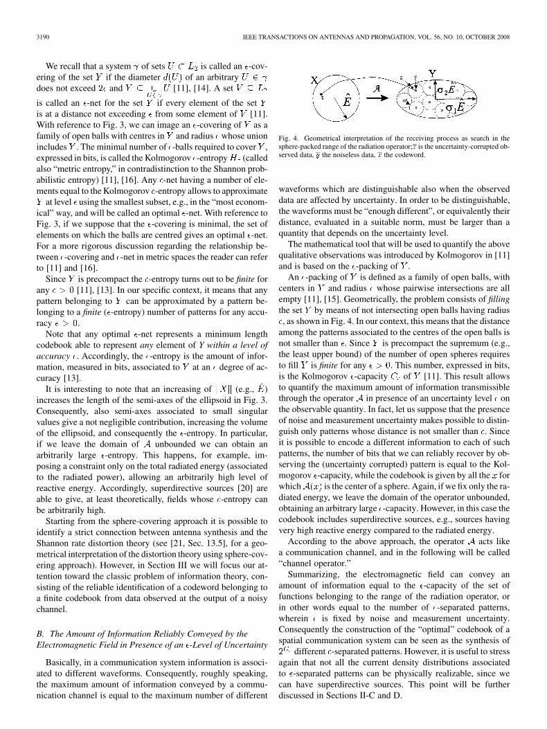
Fig. 4. Geometrical interpretation of the receiving process as search in thesphere-packed range of the radiation operator;z is the uncertainty-corrupted ob-served data, y the noiseless data, x the codeword.

waveforms which are distinguishable also when the observeddata are affected by uncertainty. In order to be distinguishable,the waveforms must be “enough different”, or equivalently theirdistance, evaluated in a suitable norm, must be larger than aquantity that depends on the uncertainty level.

The mathematical tool that will be used to quantify the abovequalitative observations was introduced by Kolmogorov in [11]and is based on the -packing of .

An -packing of is defined as a family of open balls, withcenters in and radius whose pairwise intersections are allempty [11], [15]. Geometrically, the problem consists of fillingthe set by means of not intersecting open balls having radius, as shown in Fig. 4. In our context, this means that the distance

among the patterns associated to the centres of the open balls isnot smaller than . Since is precompact the supremum (e.g.,the least upper bound) of the number of open spheres requiresto fill is finite for any . This number, expressed in bits,is the Kolmogorov -capacity of [11]. This result allowsto quantify the maximum amount of information transmissiblethrough the operator in presence of an uncertainty level onthe observable quantity. In fact, let us suppose that the presenceof noise and measurement uncertainty makes possible to distin-guish only patterns whose distance is not smaller than . Sinceit is possible to encode a different information to each of suchpatterns, the number of bits that we can reliably recover by ob-serving the (uncertainty corrupted) pattern is equal to the Kol-mogorov -capacity, while the codebook is given by all the forwhich is the center of a sphere. Again, if we fix only the ra-diated energy, we leave the domain of the operator unbounded,obtaining an arbitrary large -capacity. However, in this case thecodebook includes superdirective sources, e.g., sources havingvery high reactive energy compared to the radiated energy.

According to the above approach, the operator acts likea communication channel, and in the following will be called“channel operator.”

Summarizing, the electromagnetic field can convey anamount of information equal to the -capacity of the set offunctions belonging to the range of the radiation operator, orin other words equal to the number of -separated patterns,wherein is fixed by noise and measurement uncertainty.Consequently the construction of the “optimal” codebook of aspatial communication system can be seen as the synthesis of

different -separated patterns. However, it is useful to stressagain that not all the current density distributions associatedto -separated patterns can be physically realizable, since wecan have superdirective sources. This point will be furtherdiscussed in Sections II-C and D.


Upper bound and lower bound of the -entropy and -capacityof the channel in space can be obtained directly from the ge-ometrical interpretation in terms of sphere-packing and sphere-covering, considering ellipsoids having respectivelydimensions and dimensions, wherein denotesthe number of singular values . Taking into account thatthe th semiaxis of the ellisposids is long, and supposing

, we have [18]

(3)

wherein is the -entropy (related to uncertainty level).The concepts of -entropy and -capacity are extremely useful

tounderstandthe theoretical limitations in theamountof informa-tion contained and transmissible by electromagnetic systems, buttheir application in practical electromagnetic problems is cum-bersome. In fact, in electromagnetic theory the field is usuallyrepresentedbysuperpositionofsuitablybasis functions.Thisnat-urallysuggestsadifferentapproachwhichiscloser toclassic toolsused in electromagnetic theory for the approximation of , e.g.,the identificationof abasis with the minimum numberofelementswhich allows a linear approximation of any element of withinan error . Such a basis is called an “optimal basis.”

In order to clarify the importance of such a basis, let us sup-pose that the dimension of an optimal basis is . Any elementof is identified (at an -level of approximation) by the coef-ficients of the linear expansion. Furthermore, since the basis ofthe expansion is optimal, is also the minimum number of pa-rameters required to identify any element of y within an approx-imation level using a linear approximation, and consequentlyfixes the number of variables to identify the “state” of the fieldradiated on (e.g., its spatial distribution) at a level of approx-imation . Accordingly, the dimension of an optimal basis isthe number of degrees of freedom of at the -level of approx-imation (called in the following) [13].

The problem of identifying an optimal space, and hencethe , can be rigorously solved by means of theKolmogorov -width (or -diameter) of the set .

The Kolmogorov - width of in is the infimum ofthe distance between and any -dimensional subspace of[17]. Note that the minimum such that the -width is notgreater than fixes also the minimum dimension of linear sub-spaces approximating the elements of at level of accuracy ,and hence the of . In particular, with reference tothe Hilbert Schmidt decomposition in (2), the -width of isequal to , while an optimal subspace is given by the

[17]. Accordingly. the the ofis equal to the number of singular values greater than ,

e.g.,Inmanycases thesingularvaluesof thecompactoperatorshave

a step-like behavior, with a rapid decrease after the knee. In thiscaseall thesingularvalueswhoseindexislargerthanaquantity, let

be, arenegligible foranypractically reasonableuncertaintylevel . Consequently, the is scarcely dependent on

. The relevant consequence is that in this case we can makereferencetotheNumberofDegreesofFreedomwithoutexplicitlyindicating the approximation level , introducing the concept of

[13]. Furthermore, with reference to (3), we can note thatin this case and the -entropynumber of elements at the center of the -spheres in the sphere-coveringaswellas the -capacitynumberofelementsat thecenterof the -spheres in the sphere-packing belong to andimensional space.

Now, let us consider the probabilistic Shannon theory, inwhich signal and noise are stochastic quantities. The connec-tions between Kolmogorov and Shannon approach are discussedin [11]. For our purpose, we can note that Fig. 4 suggests astraightforward parallelism between the Kolmorogov -ca-pacity approach and the approach used in Information Theoryfor bandlimited channels corrupted by additive white Gaussiannoise (see for example [21, Sec. 10.1] for a sphere-packinginterpretation of the Shannon capacity). Paralleling the classicInformation Theory approach, we can use the Hilbert-Schmidtdecomposition of the channel operator to decompose thechannel operator in parallel Gaussian channels. Inparticular in the Appendix at the end of this paper it is shownthat in a statistical approach each singular function associatedto the first NDF singular values of the channel operator ispotentially able to convey statistically independent informationalong the communication channel.

As last observation, it is important to stress again the para-mount importance of the concept of the . From a physicalpoint of view, the is the minimum number of parametersthat allows to identify any element of , e.g., any configura-tion of the electromagnetic field on the observation manifold,within a level of approximation suitable for practical applica-tions, using a linear approximation. Since the spatial distributionof the field is uniquely identified by parameters, we canassociate independent information to each of these pa-rameters. Accordingly, while the -capacity measures the max-imum number of distinguishable signals, the gives theeffective number of dimensions of the space in which these sig-nals lie, e.g., the dimension of the “signal space.” Consequently,the NDF has a fundamental role both in pattern approximationand in the information conveyed by the field suggesting a prac-tical way to identify the connection between these two prob-lems. This way will be followed in Section III. An intuitive dis-cussion on the role of the in pattern approximation andinformation transmission is also reported in [22].

C. Some Examples of Spatial Channel Operators

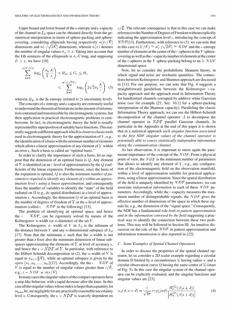
In order to discuss the properties of the spatial channel op-erator, let us consider a 2D scalar example regarding a circulardomain D limited by a circumference having radius , and acircular observation curve having the same center of (insetof Fig. 5). In this case the singular system of the channel oper-ator can be explicitly evaluated, and the singular functions andsingular values are [23]

(4)


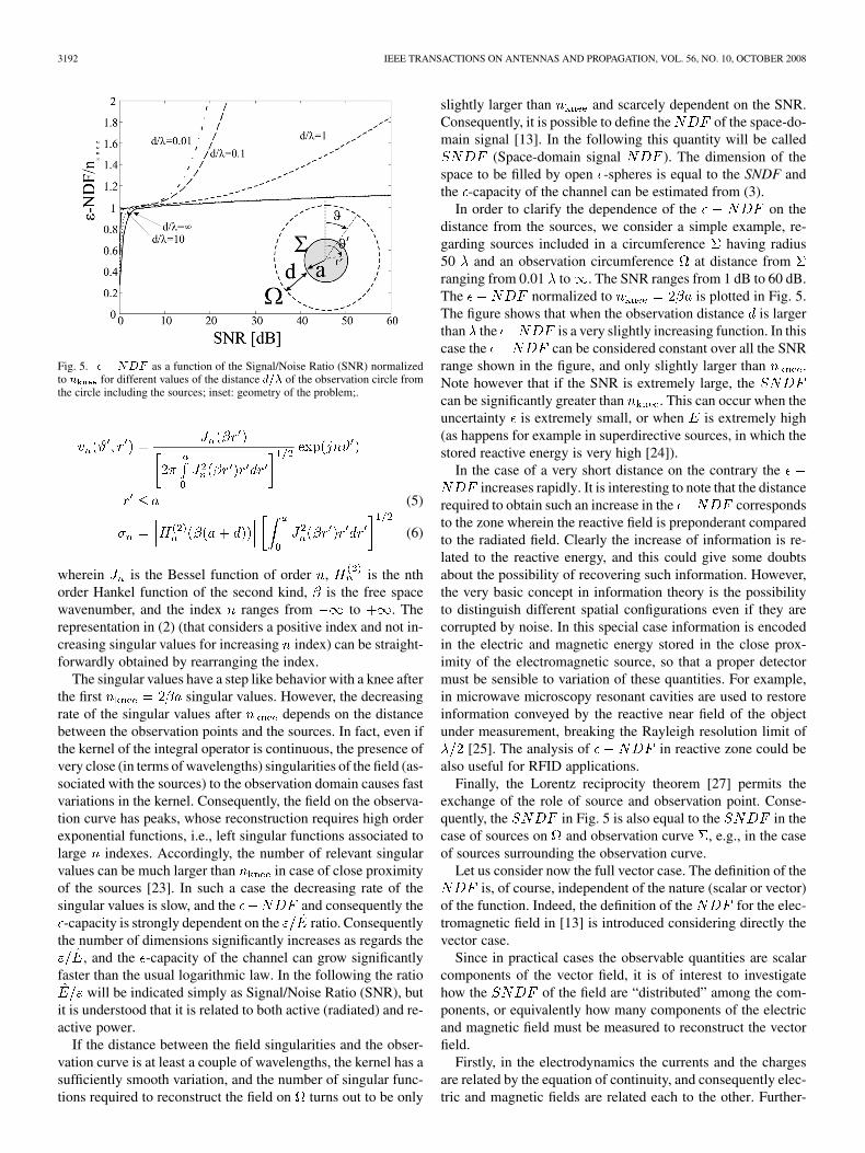
Fig. 5. � � NDF as a function of the Signal/Noise Ratio (SNR) normalizedto n for different values of the distance d=� of the observation circle fromthe circle including the sources; inset: geometry of the problem;.

(5)

(6)

wherein is the Bessel function of order , is the nthorder Hankel function of the second kind, is the free spacewavenumber, and the index ranges from to . Therepresentation in (2) (that considers a positive index and not in-creasing singular values for increasing index) can be straight-forwardly obtained by rearranging the index.

The singular values have a step like behavior with a knee afterthe first singular values. However, the decreasingrate of the singular values after depends on the distancebetween the observation points and the sources. In fact, even ifthe kernel of the integral operator is continuous, the presence ofvery close (in terms of wavelengths) singularities of the field (as-sociated with the sources) to the observation domain causes fastvariations in the kernel. Consequently, the field on the observa-tion curve has peaks, whose reconstruction requires high orderexponential functions, i.e., left singular functions associated tolarge indexes. Accordingly, the number of relevant singularvalues can be much larger than in case of close proximityof the sources [23]. In such a case the decreasing rate of thesingular values is slow, and the and consequently the-capacity is strongly dependent on the ratio. Consequently

the number of dimensions significantly increases as regards the, and the -capacity of the channel can grow significantly

faster than the usual logarithmic law. In the following the ratiowill be indicated simply as Signal/Noise Ratio (SNR), but

it is understood that it is related to both active (radiated) and re-active power.

If the distance between the field singularities and the obser-vation curve is at least a couple of wavelengths, the kernel has asufficiently smooth variation, and the number of singular func-tions required to reconstruct the field on turns out to be only

slightly larger than and scarcely dependent on the SNR.Consequently, it is possible to define the of the space-do-main signal [13]. In the following this quantity will be called

(Space-domain signal ). The dimension of thespace to be filled by open -spheres is equal to the SNDF andthe -capacity of the channel can be estimated from (3).

In order to clarify the dependence of the on thedistance from the sources, we consider a simple example, re-garding sources included in a circumference having radius50 and an observation circumference at distance fromranging from 0.01 to . The SNR ranges from 1 dB to 60 dB.The normalized to is plotted in Fig. 5.The figure shows that when the observation distance is largerthan the is a very slightly increasing function. In thiscase the can be considered constant over all the SNRrange shown in the figure, and only slightly larger than .Note however that if the SNR is extremely large, thecan be significantly greater than . This can occur when theuncertainty is extremely small, or when is extremely high(as happens for example in superdirective sources, in which thestored reactive energy is very high [24]).

In the case of a very short distance on the contrary theincreases rapidly. It is interesting to note that the distance

required to obtain such an increase in the correspondsto the zone wherein the reactive field is preponderant comparedto the radiated field. Clearly the increase of information is re-lated to the reactive energy, and this could give some doubtsabout the possibility of recovering such information. However,the very basic concept in information theory is the possibilityto distinguish different spatial configurations even if they arecorrupted by noise. In this special case information is encodedin the electric and magnetic energy stored in the close prox-imity of the electromagnetic source, so that a proper detectormust be sensible to variation of these quantities. For example,in microwave microscopy resonant cavities are used to restoreinformation conveyed by the reactive near field of the objectunder measurement, breaking the Rayleigh resolution limit of

[25]. The analysis of in reactive zone could bealso useful for RFID applications.

Finally, the Lorentz reciprocity theorem [27] permits theexchange of the role of source and observation point. Conse-quently, the in Fig. 5 is also equal to the in thecase of sources on and observation curve , e.g., in the caseof sources surrounding the observation curve.

Let us consider now the full vector case. The definition of theis, of course, independent of the nature (scalar or vector)

of the function. Indeed, the definition of the for the elec-tromagnetic field in [13] is introduced considering directly thevector case.

Since in practical cases the observable quantities are scalarcomponents of the vector field, it is of interest to investigatehow the of the field are “distributed” among the com-ponents, or equivalently how many components of the electricand magnetic field must be measured to reconstruct the vectorfield.

Firstly, in the electrodynamics the currents and the chargesare related by the equation of continuity, and consequently elec-tric and magnetic fields are related each to the other. Further-


more, the field outside a surface including all the sources isuniquely defined by the two tangential components of the elec-tric (or magnetic) field on the surface due to the uniqueness the-orem. Consequently, in this case it is possible to estimate the

of the (vector) electromagnetic field by evaluating theof two (tangential) components of the electric field on

the observation surface.Let us consider a simple example consisting of electromag-

netic sources spatially limited by a spherical surface havingradius , and a spherical observation manifold having radius

concentric to . The field outside can be expandedin spherical harmonics [27] that represent an optimum basis in

. Only a finite number of spherical harmonics are required torepresent the field on within a finite approximation. Such anumber of harmonics is the of the field at the requiredlevel of approximation [28]. The number of spherical harmonicsrequired to represent the field on , and hence the , fora not superdirective source tends to for andfor an observation surface at least a couple of wavelengths from

[27]. In particular, the field on is represented by means ofradial TE and radial TM modes, that can

be reconstructed from the knowledge of the two componentsof the electric (or magnetic) field tangent to , each of themcharacterized by number of degrees of freedom. The

of the vector field is consequently obtained by the sumof the number of degrees of freedom of these two scalar com-ponents.

Note that when the radiating system becomes electricallysmall the does not tend to zero, and theformula cannot be applied. This is due to the fact that anyelectrically small antenna acts like a superdirective source [27],increasing the reactive energy compared to the radiated energywhen . Even if theoretically no upper bound exists forthe , the fast increasing of the Q factor limits in practicethe potentially useful modes to the lowest six ones [29].

As last observation, the field radiated by an electromagneticsource having finite size is an analytic function on the observa-tion domain [26], and hence has an infinite number of degreesof freedom. However in practical instances we can observe onlythe portion of this function falling on the observation domain.Furthermore, also if we extend the observation domain to thewhole space, we do not have access to the analytic continua-tion of the observed field. In practice, we are able to observea noise-corrupted analytic function only on an observation do-main having finite extension. The consequence of this lack ofknowledge is that an upper-bound exists for the number of de-grees of freedom associated to the spatial domain even if weextend the observation domain to the whole space [5]. For a notsuperdirective radiating system, such an upper-bound is of theorder of [31], wherein is the areaof the smallest convex surface including the source, and is thewavelength.

The existence of an upper-bound for the spatial is animportant difference between space-domain and time-domaincommunication systems. In fact, since it is possible to observea (temporal) signal for an arbitrarily long temporal interval, noupper-bound exists for the in time domain communica-tion systems.

D. An Example of Space-Time Channel Operator

In Section II-A the theory was explained with special ref-erence to the radiation operator, e.g., considering a “pure spa-tial” channel [5], in which information are encoded in spatialvariation of the electromagnetic field on the observation sur-face. Of course the theory is general, and other channel op-erators can be considered. Operators working on time-domainfunctions give the classic time-domain communication chan-nels, while operators working on signals defined both in timedomain and space domain give the space-time communicationchannels used in MIMO communication system analysis. How-ever, Hilbert-Shmidt decomposition of the operators, and in par-ticular operators working on functions defined in the space-timedomain, is analytically cumbersome. In this Section a simpleupper bound for the channel capacity of space-time communi-cation systems is presented, using band limitation approxima-tion of the space-time received signal. The use of band-limitedapproximation is advantageous in our context since there is alarge and well established literature on the optimal basis and onthe for this class of functions [33]. In particular, the re-sults showed in this section are a straightforward extension ofthe results regarding the well-known time-domain bandlimitedchannel corrupted by a stochastic process modelled as additivewhite Gaussian noise (AWGN) [21].

In the following the TNDF, SNDF and STNDF will denote re-spectively the of the time-domain signal, of the space-do-main signal (e.g., the spatial distribution of the electromagneticfield on the observation surface) and of the space-time-domainsignal.

Let us consider a time-domain bandlimited signal having(time-domain) bandwidth (wherein and arethe minimum and maximum frequency of the signal), radiatedby not superdirective sources placed inside a convex surface

, and observed on a curve , on which we introduce a properparameterization , wherein is the curvilinear abscissaalong . As discussed in [30], [31], for each frequency ofthe temporal signal we can identify a spatial bandwidthfor the field observed on . For the sake of simplicity, asa first step in this section we suppose that the spatial band-width can be considered flat in the time bandwidth , e.g.,

. Accordingly, the field can be expandedin the Whittaker-Kotel’nikov-Shannon (WKS) sampling series[32]

(7)

wherein is the (time-domain) field observed at time inthe point of coordinate along the observation curve, is re-lated to a suitable phase function subtracted from the field [32],

is the free space light velocity, and the number of (spatial) sam-ples in the representation is practically equal to the .

The formula in (7) gives a simple explanation regarding thelimits of space-time communication systems. The value of thefield (and consequently also of any signal carried by the elec-tromagnetic field) in a point of the observation manifold canbe obtained by a linear combination of the field in other points


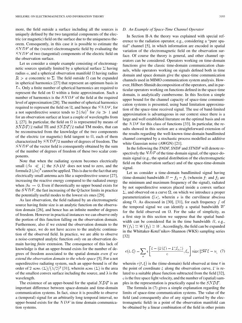
Fig. 6. The space-bandlimited time-bandlimited AWGN channel.

of the observation manifold provided that a proper time shift istaken into account. The number of positions that carry indepen-dent information is finite, and equal to the fornon superdirective sources, wherein is the length of the ob-servation curve. In practice the is an upperbound forthe number of SISO subchannels that can be obtained for anyconfiguration of TX antennas spatially limited by and RX an-tennas placed on [5].

Let us suppose that the received signal is corrupted by AWGNnoise having power (Fig. 6). The observable quantity is con-sequently: wherein is the(space-time) bandlimited AWGN affecting the observed data.Under the hypothesis that the time-signals are bandlimited withbandwidth and observation interval , the received signal canbe represented by a double WKS series, in which the number oftemporal samples is essentially [33] and thenumber of spatial samples is essentially [13].The space-time number of degrees of freedom (STNDF) of theflat spatial-bandwidth space-time channel is .

The channel capacity (bits/s) of the space-time communi-cation system can be obtained paralleling the classic approachregarding the time-domain bandlimited channel [12], obtaining

(8)

wherein is the received average power andhas the same role of the noise spectral density defined in theclassic time-domain signal channel

Finally, we can note that the supremum of the amount of in-formation that can be transmitted along the channel in a spaceinterval and a time interval is not greater than

(9)

wherein is the energy of the signal.As discussed in Section II-C, it is theoretically possible to

increase the in a spatial interval beyond the stan-dard value of by means of superdirective radiating sys-tems [4]. Since superdirective sources have small bandwidth, ifwe increase the SNDF significantly above , we also obtaina decrease of the TNDF, so that the most important quantity ina communication system is the STNDF.

Let us consider now the case of a space-time channel having(time) bandwidth with an average power constraint

. Following the classic approach of Information Theory, the

channel is divided into a large number of narrow sub-channelshaving bandwidth , in which the spatial bandwidth can be con-sidered practically constant. The spatial bandwidth is a linearfunction of the frequency, and will be expressed as ,wherein the constant is the spatial bandwidth for unit fre-quency , while , and do not depend on the frequency[31].

The channel capacity can be obtained by maximizing the ex-pression

(10)

with the constraint

(11)

Using the method of Lagrange multipliers we obtain that thechannel capacity is

(12)

wherein and . Comparing (12)multiplied by and (9), we obtain the value of the

. Again, the STNDF is the product of two quanti-ties, the TNDF, equal to 2BT, and a quantity, , thatrepresents the SNDF of the wide-band communication system.

III. APPLICATION TO ANTENNAS

A. A Unified Approach to Classic, Adaptive and MIMOAntennas

As discussed in Section II-B, there is a strong connection be-tween the “degree of complexity” of a set of functions, e.g., the

defined as the infimum of the number of functions re-quired to represent the set of functions within a given accuracy,and the “amount of information” that the set of functions canconvey in presence of noise. Broadly speaking, the is a“money” that can be spent in two different ways: to obtain afunction that concentrates the energy in some desired intervals,or to send statistically independent information. In the first casethe degrees of freedom are used in the “approximation theory”sense, while in the second case they are used in the “communi-cation theory” sense.

This is indeed exactly what happens in antenna synthesis. Inorder to clarify the double role that the of the field canplay, let us consider an antenna consisting in electromagneticcurrents having a finite spatial extension as in Fig. 1. As firststep, we suppose that the source radiates in the free space, andonly one state of polarization is used to transmit information.In the classic synthesis approach the receiving antenna is in thefar-field region at a distance such that it is seen as point-like fromthe radiating system. In presence of only AWG noise, under


the hypothesis that the receiving antenna aperture is unitary, thechannel capacity is

(13)

wherein is the power at the input of the transmitting antenna,is the directivity (supposed equal to the antenna gain) of the

transmitting antenna, is the path loss, the noise power, andthe bandwidth of the time-domain signal. In order to show the

role played by the in the channel capacity, let us considera sphere centered in the transmitting antenna whose radius tendsto infinity as observation surface. By expanding the radiationoperator (1) as in (2) we identify the of the field. Note thatthe choice of the observation surface maximizes the available

. In fact, any further degree of freedom is associated tothe analytical continuation of the field, e.g., to singular valuesof the radiation operator that are negligible in the case of notsuperdirective source. This will be called in thefollowing.

The goal of the antenna designer is to set the coefficients ofthe currents whose distributions are given by the left singularfunctions, in order to maximize the channel capacity. This goalcan be reached by increasing the directivity of the antenna. In-deed, there is a strict relationship between the directivity and thenumber of singular functions used in the synthesis problem [24].For example, the maximum directivity of a source enclosed ina sphere having radius is proportional to the number of sin-gular values (in the specific case the spherical harmonics) usedto synthesize the pattern [34]. The practical limitation of the di-rectivity of antennas is due to the fact that only a finite number ofsingular functions can be effectively used in the synthesis [20],or equivalently that the effective is finite. For example, inthe case of spherical source discussed at the end of Section II-B,the directivity of the radiating system is practically limited toalmost [34]. By using singular functions associated tosingular values after the knee we can increase the directivity atany desired value. However, in this case we have a superdirec-tive source. Among the many well known problems regardingthe superdirective sources, we can note that the bandwidth ofthe system decreases. Since an increase of the directivity givesonly a logarithmical increase of the channel capacity, while a de-crease of the bandwidth gives a linear decrease of the channelcapacity, generally we would obtain a decrease of the channelcapacity using superdirective sources even if we were able tokeep the antenna losses at a negligible level.

Summarizing, in the above example all the availableare used to obtain a pattern that maximizes the directivity.

Let us suppose that the we must synthesize a receiving an-tenna in presence of a number of interference signals modelledas AWGN. In this case it is advantageous to filter out the interfer-ence signals in order to increase the Signal/Noise ratio. In orderto reach this goal, a number of available degrees of freedom isused to synthesize nulls toward the directions of the interferencesignals. Again, the available limits the performance ofthe system, both in terms of maximum number of interferencesignals that can be filtered out, and in terms of tradeoff betweenthe directivity and the number of nulls of the pattern. Clearly,

the maximization of the channel capacity is obtained by max-imizing the term inside the logarithm function of the channelcapacity expression. This is exactly the goal of optimal beam-forming algorithms, like Widrow or Howells-Applebaum algo-rithms [35], used in the adaptive antennas.

It is interesting to note that adaptive antennas are used in adouble role. On a side, they are used to synthesize a pattern withnulls toward the angle of arrivals (AoA) of the interferences, onthe other side they are used to identify the AoA of the signals,e.g., to extract information from the environment. A well knownresult is that an array of radiating elements can identify theAoA of up to uncorrelated signals. However, the identifi-cation of the AoA is related to the possibility to distinguish thesubspace of the received signals correlation matrix associatedto the signal (the signal space) from the subspace associated tothe noise (the noise space) [35]. If we increase above the

, the spreading of the singular values associated to thesignal space tends to fast increase. In this case the presence ofnoise tends to “cover” some signal space eigenvalues, makingimpossible to divide the signal space from the noise space, andconsequently also the identification of the AoA of the signals.Accordingly, theoretically we do not have limitation regardingthe number of signals that we can identify, but when the numberof (uncorrelated) signals becomes significantly larger than the

a situation similar to the superdirectivity occurs, so thatin practice the number of signals is limited by the electrical di-mension of the antenna. In practice we have basically the samelimitations when the antenna is used to synthesize a pattern, andwhen it is used to extract information from the environment.

Let us suppose now that we have to synthesize a transmitterantenna in the case of not point-like receiving antenna. By ex-panding the radiation operator relating the source currents andthe observation curve wherein the receiving antenna is placed,we can evaluate the available . Due to the extremal prop-erties of the singular values, the first singular function assuresthe maximum concentration of the power in the area covered bythe receiving antenna, and consequently the maximization of theargument of the logarithm in the channel capacity expression,obtaining the following bit rate:

(14)

wherein is the first singular value. This solution is known as“MIMO beamforming.”

However, we can follow a different strategy, associating sta-tistically independent information at each singular function. Forsake of simplicity, let us suppose that all the relevant singularvalues of the radiating operator are constant. In this case we havethat

(15)

that is larger than the bit rate in (14) in the case of sig-nificantly greater than zero (note that in the case of not constantsingular values the maximization of the capacity requires to dis-tribute the available average power among the different spatial


subchannels associated to the singular values; the solution of theproblem is given by the so called water-filling algorithm [38]).This strategy is followed in spatial multiplexing MIMO systems.Accordingly, in practice a MIMO antenna is a radiating systemthat conveys statistical independent information on more thanone spatial degree of freedom.

Summarizing, if the NDF of the field incident on the receivingantenna is only one, the maximization of the received power (orof the SINR in presence of not cooperative interference sources)gives also the maximization of the bit rate, since it is not pos-sible to distinguish different radiated field spatial configuration,and information can be encoded only by means of temporalvariations. In this case, classic antenna synthesis based on an“energetic” approach allows also the maximization of the bitrate. However, if the incident field has more than one degree offreedom, the maximization of the received power does not as-sure maximization of the bit rate. In this case it is more advan-tageous to use the available degrees of freedom of the incidentsignal to transmit statistically independent information, e.g., toencode information also by “modulating” the spatial distribu-tion of the field. Since the distance between the transmitting andreceiving antennas is very large in terms of wavelengths, thelocal incident field on the receiving antenna is usually a planewave. Furthermore, information is usually associated to onlyone of the two independent polarizations of the vector field. Inthis case the incident field has only one degree of freedom andthe classic synthesis approach, based on an “energetic” point ofview, gives the same results of an antenna synthesis based onan informational point of view (e.g., whose goal is not to con-trol the distribution of the radiated power in the space, but onlyto maximize the bit rate). Note however that if we are able touse both the polarizations of the incident plane wave, we havetwo degrees of freedom of the field also in the classic free-spacefar-field link. Accordingly, the double-polarized antennas are aparticular case of MIMO antennas [22].

A further important case regards antennas operating incomplex environments, e.g., environments containing a largenumber of scattering objects. In fact, in case of dense scatteringenvironment the incident field is the superposition of a largenumber of plane waves, and hence has more than one degreeof freedom. From a mathematical point of view, the channeloperator is an integral operator like (1), wherein the Green’sfunction must be calculated in presence of scattering objects.The integral operator is compact provided that the observationcurve does not intersect sources of the field, and the generaldiscussion regarding the does not change. However,due to the presence of the secondary sources associated to thescattering objects, the on a given observation manifoldis usually higher than the on the same manifold in thecase of absence of scatterers. Consequently, the presence ofscattering objects allows to have a value of higher thanone also on observation domains having small (only somewavelengths) length, as happens in practical MIMO applica-tions.

Of course, the in absence of scatterers is an upperbound for the of the field, provided that the scatteringproperties of the objects do not change. In fact, the possibilityto control the scattering properties of the objects gives further

degrees of freedom to modify the field configuration. A prac-tical application of controllable scattering objects is representedby MIMO parasitic antennas [36], [37]. In these antennas par-asitic elements terminated on electronically controllable loadsare used as low cost solution to increase the of the fieldcompared to the of the radiating system consisting of thesole active antennas.

B. Application of the Double Role of the NDF in AntennaSynthesis

According to the above observations, in complex environ-ment it is advantageous to modify classical approaches in orderto use the available NDF of the received field to send statisti-cally independent information. Let us consider an example ofsuch an approach. One of the techniques proposed in the frame-work of personal communication system is the spatial filteringfor interference reduction (SFIR), consisting in imposing themaximum of the radiation pattern of the antenna toward the sub-scriber of interest, and imposing nulls in the direction of inter-ference sources using adaptive antennas. In terms of degrees offreedom, SFIR uses some degrees of freedom to impose nulls ofthe field pattern, and the remaining ones to maximize the powerreceived by the subscriber of interest.

Let us suppose that the system works in a dense scatteringenvironment, as often happens. In this case we can use part of thedegrees of freedom to impose nulls of the field on the elementsof the antenna that we do not want to illuminate, let us call itantenna “D,” and use the remaining degrees of freedom to sendstatistically independent information to the antenna of interest,let us call it antenna “B,” obtaining a MIMO system with nullconstraint. The transmitting antenna will be called antenna “A.”

We consider a preliminary step, in which A and D coop-erate to identify the channel matrix from A to D. In the classicMIMO matrix notation [38], [39], we have , wherein

is the vector collecting the signals at the input ofthe transmitting array A, having radiating elements,

is the vector collecting the signals at the input of the re-ceiving array D, having radiating elements, andis the channel matrix. In order to null the field on D, we mustimpose . The projector onto the nullspace of is

, whereinand are the right singular vectors of thesingular value decomposition (SVD) of associated to singularvalues of the matrix having zero value [40]. Then the transmis-sion toward the antenna B having M elements starts. Using thestandard MIMO notation, in absence of null constraint we have

, wherein is the vector collecting the signalsat the input of the transmitting array is the vectorcollecting the signals at the input of the receiving array B, and

is the channel matrix.In order to assure the null toward D, we consider the subset

of lying in the null of . Consequently, the input of the arrayA is the vector , and the input-output relationshipbecomes . Accordingly, in presence of null con-straint we have an equivalent channel matrix .Using classic MIMO approach [38], [39] we are able to maxi-mize the bit rate toward B, without interfering with D.


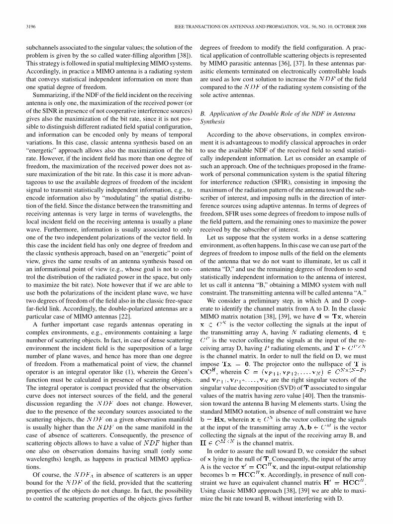
Fig. 7. Channel capacity in the case of MIMO system with null constraint (solidline), MIMO system without null constraint (dotted line) and MIMO beam-forming with null constraint (dashed line); in the inset a scheme of the geometryof the problem is drawn; the large filled circles represent the scattering objects,randomly placed.

In the following a simple 2-D example is reported. The sce-nario consists in 40 2-D point-like scatterers placed in an area

, and an array (antenna A) consisting of ele-ments placed along the axis, with the central element placedin (see inset of Fig. 7). The antenna D is alinear array of elements, parallel to antenna A with thecentral element placed in . Then the averagechannel capacity considering an array (antenna B) parallel to theantenna A and having elements, whose central oneis placed in with ranging between 4 and 45 ,is evaluated. The average channel capacity is evaluated consid-ering 100 different random scenarios. The contribution of theline of sight (LOS) between the transmitting and the receivingarray is subtracted, and only the scattered field is consideredin the numerical simulations. The channel capacity, evaluatedin the case of uniform power distribution between the elementsof the transmitting antennas (e.g., no waterfilling solution), isplotted in Fig. 7 as solid line. In the same figure the channelcapacity in the case of MIMO system without null constraintis plotted as dotted line, while the MIMO beamforming case,that maximizes the received energy with the null constraint, isplotted as dashed line. The plots confirm that the hybrid “en-ergetic/informational” solution allows to assure the null con-straint, with better performance compared to the pure “ener-getic” solution (e.g., the dashed line).

C. Application of the Double Role of the NDF in AntennaCharacterization

A further simple example of the use of the “double role” ofthe NDF is in the MIMO antenna characterization.

As preliminary step, let us recall that a well establishedmethod for characterization of classic antennas is based onnear-field measurements. In practice, this technique allows toidentify the of the antenna under test from measure-ments of radiated power density [41].

Now let us consider the characterization of a MIMO antenna.From an informational point of view, the quantity of interest is

the amount of statistically independent information that we canobtain at the output of the MIMO antennas. This goal can bereached by analyzing the eigenstructure of the covariance matrixof the output signals, under the classic hypothesis of Gaussiandistribution of the signals.

Unfortunately, such a quantity depends not only on our an-tenna, but on the whole communication system, e.g., also on thetransmitting antenna and on the environment. In order to iden-tify a quantity that allows to characterize the antenna itself froman informational point of view, we can use the double role ofthe SNDF.

In fact, according to the observations outlined in this paper,a MIMO antenna is basically a (usually linear) operator thattransforms a signal belonging to a theoretically infinite di-mensional space (the incident electromagnetic field) into asignal belonging to a finite dimensional space (the signals atthe output of the elements of the antenna). The number ofdimensions of the “output space” (e.g., the received signalspace) is equal to the number of elements of the MIMOantenna, let be, while the number of (effective) dimen-sions of the “input space” is equal to the SNDF. This numbercannot be larger than the of the field radiated by theantenna in the whole space, that has been denoted as .Accordingly, for a fixed frequency the antenna operator iscompletely characterized (at a fixed degree of accuracy) bya table of elements. This table, that can beobtained from standard near-field measurements [41], is anintrinsic property of the antenna, and allows to characterizethe information content associated to the received signal spacefor any communication channel configuration.

A simple example of application of the above observationsregards a MIMO antenna having elements, and spatially lim-ited by a spherical surface having radius . The field radiated byeach element of the antenna, with the other elements terminatedon the working loads, is expanded in spherical har-monics, as discussed in Section II-C. The table ofcoefficients allows to evaluate the covariance matrix of the re-ceived signals, and consequently also the channel capacity, afterfixing the environmental model. This approach was followedby Gustafsson and Nordebo in the case of Rayleigh environ-ment (e.g., the so called rich scattering environment) [10]. Notethat the possibility of characterizing the antenna from an infor-mational point of view using methods (e.g., near-field measure-ments) currently used to characterize the antenna from an “ener-getic” point of view is a practical application of the double roleof the degrees of freedom.

This observation allows to extend the well established liter-ature on the characterization of classic antennas to MIMO an-tennas. As an example, a widely adopted method is to samplethe field radiated by the antenna using near-field measurementsystems. In particular, according to [31], [41], the field radiatedby each element of the MIMO antenna can be represented by aproper sampling representation whose number of terms is onlyslightly larger than the . This suggests to sample the fieldin these points using classic near-field measurement systems.Then the field is interpolated in a large number of directions,and the correlation matrix is numerically evaluated by consid-ering uncorrelated waves impinging from these directions.


Fig. 8. Eigenvalues of the correlation matrix for a MIMO cube antennain the case of uncorrelated signals impinging from an half-space.

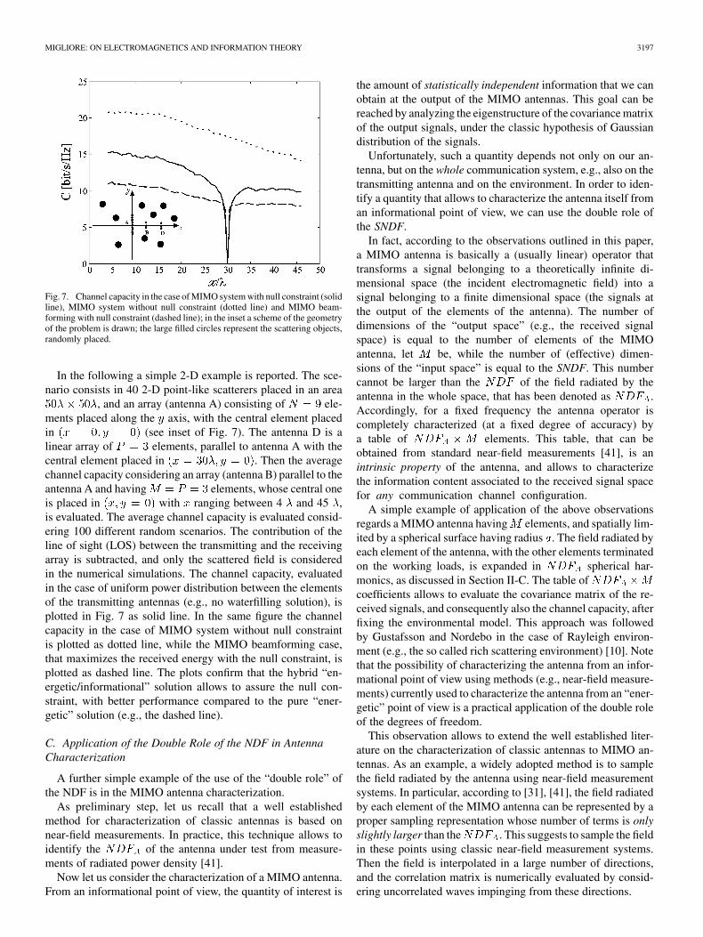
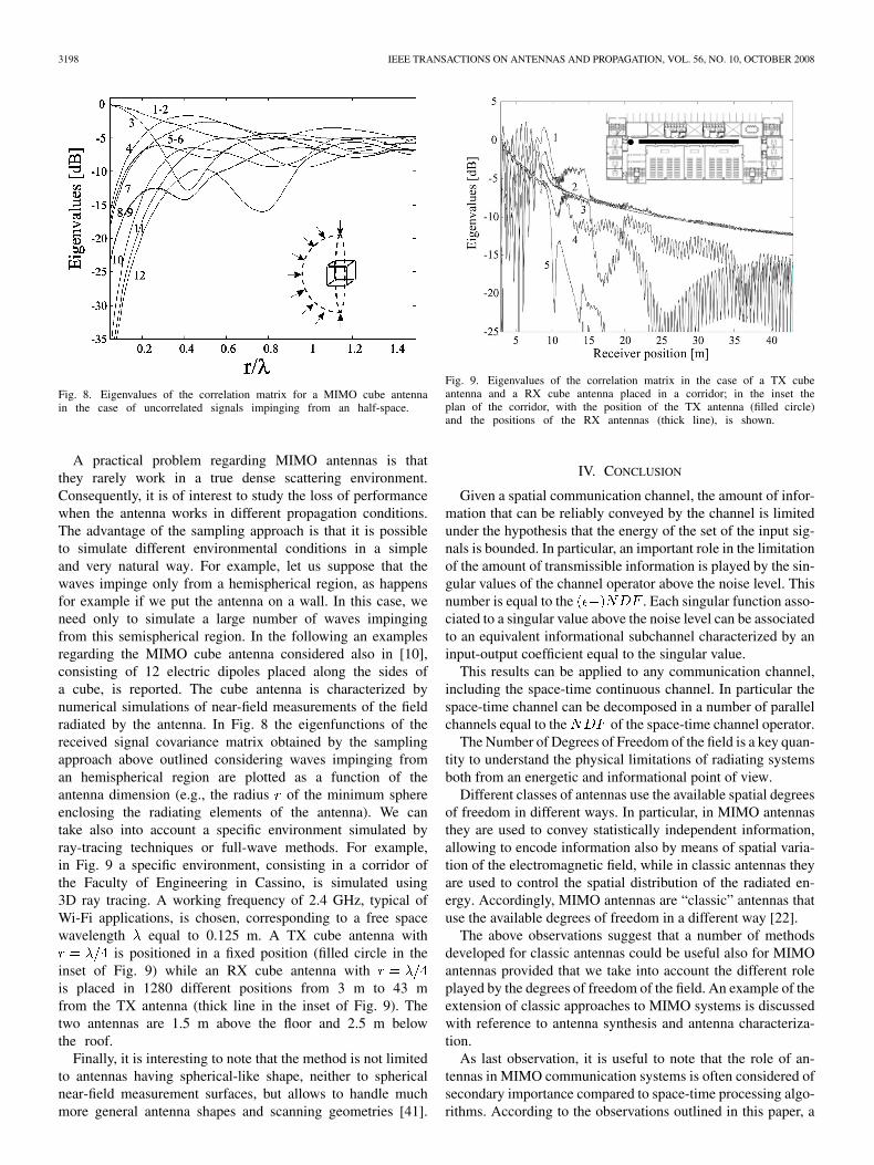
A practical problem regarding MIMO antennas is thatthey rarely work in a true dense scattering environment.Consequently, it is of interest to study the loss of performancewhen the antenna works in different propagation conditions.The advantage of the sampling approach is that it is possibleto simulate different environmental conditions in a simpleand very natural way. For example, let us suppose that thewaves impinge only from a hemispherical region, as happensfor example if we put the antenna on a wall. In this case, weneed only to simulate a large number of waves impingingfrom this semispherical region. In the following an examplesregarding the MIMO cube antenna considered also in [10],consisting of 12 electric dipoles placed along the sides ofa cube, is reported. The cube antenna is characterized bynumerical simulations of near-field measurements of the fieldradiated by the antenna. In Fig. 8 the eigenfunctions of thereceived signal covariance matrix obtained by the samplingapproach above outlined considering waves impinging froman hemispherical region are plotted as a function of theantenna dimension (e.g., the radius of the minimum sphereenclosing the radiating elements of the antenna). We cantake also into account a specific environment simulated byray-tracing techniques or full-wave methods. For example,in Fig. 9 a specific environment, consisting in a corridor ofthe Faculty of Engineering in Cassino, is simulated using3D ray tracing. A working frequency of 2.4 GHz, typical ofWi-Fi applications, is chosen, corresponding to a free spacewavelength equal to 0.125 m. A TX cube antenna with

is positioned in a fixed position (filled circle in theinset of Fig. 9) while an RX cube antenna withis placed in 1280 different positions from 3 m to 43 mfrom the TX antenna (thick line in the inset of Fig. 9). Thetwo antennas are 1.5 m above the floor and 2.5 m belowthe roof.

Finally, it is interesting to note that the method is not limitedto antennas having spherical-like shape, neither to sphericalnear-field measurement surfaces, but allows to handle muchmore general antenna shapes and scanning geometries [41].

Fig. 9. Eigenvalues of the correlation matrix in the case of a TX cubeantenna and a RX cube antenna placed in a corridor; in the inset theplan of the corridor, with the position of the TX antenna (filled circle)and the positions of the RX antennas (thick line), is shown.

IV. CONCLUSION

Given a spatial communication channel, the amount of infor-mation that can be reliably conveyed by the channel is limitedunder the hypothesis that the energy of the set of the input sig-nals is bounded. In particular, an important role in the limitationof the amount of transmissible information is played by the sin-gular values of the channel operator above the noise level. Thisnumber is equal to the . Each singular function asso-ciated to a singular value above the noise level can be associatedto an equivalent informational subchannel characterized by aninput-output coefficient equal to the singular value.

This results can be applied to any communication channel,including the space-time continuous channel. In particular thespace-time channel can be decomposed in a number of parallelchannels equal to the of the space-time channel operator.

The Number of Degrees of Freedom of the field is a key quan-tity to understand the physical limitations of radiating systemsboth from an energetic and informational point of view.

Different classes of antennas use the available spatial degreesof freedom in different ways. In particular, in MIMO antennasthey are used to convey statistically independent information,allowing to encode information also by means of spatial varia-tion of the electromagnetic field, while in classic antennas theyare used to control the spatial distribution of the radiated en-ergy. Accordingly, MIMO antennas are “classic” antennas thatuse the available degrees of freedom in a different way [22].

The above observations suggest that a number of methodsdeveloped for classic antennas could be useful also for MIMOantennas provided that we take into account the different roleplayed by the degrees of freedom of the field. An example of theextension of classic approaches to MIMO systems is discussedwith reference to antenna synthesis and antenna characteriza-tion.

As last observation, it is useful to note that the role of an-tennas in MIMO communication systems is often considered ofsecondary importance compared to space-time processing algo-rithms. According to the observations outlined in this paper, a


MIMO antenna is basically a (usually linear) operator that trans-forms a signal belonging to a space whose effective dimensionis equal to (the incident electromagnetic field) into asignal belonging to a finite dimensional space (the signals at theoutput of the elements of the antenna). In the mapping informa-tion associated to the null space of the operator is missed, andno mathematical trick can restore such information. In order tomaximize the amount of information transmitted in the wire-less channel, the MIMO system must be “degrees of freedommatched”, in the sense that the dimension of the received signalspace must be equal to the essential dimension of the electro-magnetic field. Indeed, the antenna itself can be considered acommunication channel [42] that limits the throughput of thecommunication system.

Apart from the specific interest in space-time communicationsystems, the approach outlined in this paper can be used alsoin other fields in which space-time data processing are used.In fact, the approach can be extended to include also detectionproblems, enabling the understanding of the intrinsic limitationsof a number of emerging techniques like for example microwavetomography and MIMO RADAR [43].

APPENDIX

With reference to Fig. 2, let us suppose that the input signalis a zero mean white Gaussian stochastic process with unit

variance. Furthermore, we suppose that the observable quan-tity, let be, is the signal corrupted by zero mean additivewhite Gaussian noise with variance , e.g., .With reference to the Hilbert-Shmidt expansion of , we canobtain the classic model of parallel Gaussian channels used inInformation Theory [21], [44] using the Karhunen-Loève the-orem and expanding the input signal on the basis representedby the singular functions , obtaining the coefficients ,and the output signal and the noise on the basis representedby the singular functions , obtaining the coefficientsand . The coefficients of the input signal expansion and ofthe noise expansion are i.i.d. Gaussian processes, havingvariance equal to one, and having variance equal to .Furthermore, since(wherein is the expectation operator, is the th singularvalue and is the Kroneker symbol, equal to zero ifand equal to 1 if ) also the coefficients of the (noise-less) output signals (being Gaussian and uncorrelated) are in-dependent. The communication channel can be decomposed ina number of parallel Gaussian channels , eachof them able to transmit statistically independent information.In particular the th channel is able to convey

bits [21]. In case of step-like behaviorof the singular values, with a knee at the th singular value,

becomes negligible for , and consequentlyfor reasonable SNR only the first parallel channels areable to convey a significant amount of information. In moregeneral situations, the exact number of parallel Gaussian chan-nels that maximizes the total mutual information is given by thewater-filling algorithm.

ACKNOWLEDGMENT

The author wish to thank the anonymous referees, whose sug-gestions helped to greatly improve the clarity and readability ofthe paper.

REFERENCES

[1] L. Brillouin, Science and Information Theory. New York: AcademicPress, 1956.

[2] J. W. Wallace and M. A. Jensen, “Intrinsic capacity of the MIMO wire-less channel,” in Proc. IEEE Vehicular Tech. Conf., Vancouver, CA,Sep. 2002, pp. 701–705.

[3] A. S. Y. Poon, R. W. Brodersen, and D. N. C. Tse, “Degrees of freedomin multiple-antenna channels: A signal space approach,” IEEE Trans.Info. Theory, vol. 51, pp. 523–536, Feb. 2005.

[4] M. L. Morris, M. A. Jensen, and J. W. Wallace, “Superdirectivity inMIMO systems,” IEEE Trans. Antennas Propag., vol. 53, no. 9, pp.2850–2857, Sep. 2005.

[5] M. D. Migliore, “On the role of the number of degrees of freedom ofthe field in MIMO channel,” IEEE Trans. Antennas Propag., vol. 54,no. 2, pp. 620–628, Feb. 2006.

[6] M. D. Migliore, “Restoring the symmetry between space domain andtime domain in the channel capacity of MIMO communication sys-tems,” in Proc. AP Symp., Albuquerque, NM, Jul. 2006, pp. 333–336.

[7] S. Loyka and J. Mosig, “Information theory and electromagnetic: Arethey related?,” in MIMO Systems Technology for Wireless Communi-cation, T. Tsoulos, Ed. Boca Raton, FL: CRC & Taylor & Francis,2006.

[8] J. Xu and R. Janaswamy, “Electromagnetic degrees of freedom in 2Dscattering environment,” IEEE Trans. Antennas Propag., vol. 54, no.12, pp. 3882–3894, Dec. 2006.

[9] M. Franceschetti and K. Chakraborty, “Maxwell meets Shannon:Space-time duality in multiple antenna channels,” presented at the44th Allerton Conf. Communications Control and Computing, Mon-ticello, IL, Sep. 2006.

[10] M. Gustafsson and S. Nordebo, “Characterization of MIMO antennasusing spherical vector waves,” IEEE Trans. Antennas Propag., vol. 54,no. 9, pp. 2679–2682, Sep. 2006.

[11] A. N. Kolmogorov and V. M. Tikhomirov, “"-entropy and "-capacityof sets in functional spaces,” Amer. Math. Soc. Transl., vol. 17, pp.277–364, 1959.

[12] C. E. Shannon and W. Weaver, The Mathematical Theory of Commu-nication. Urbana and Chicago: University of Illinois Press, 1949.

[13] O. M. Bucci and G. Franceschetti, “On the degrees of freedom of scat-tered fields,” IEEE Trans. Antennas Propag., vol. AP-38, pp. 918–926,1989.

[14] D. S. Jones, Methods in Electromagnetic Wave Propagation. NewYork: Oxford Univ. Press, 1959.

[15] A. Kolmogorov and S. V. Fomine, Elements of the Theory of Functionsand Functional Analysis. New York: Dover, 1999.

[16] G. G. Lorentz, Approximation of Functions. New York: Rinehart andHolt, 1966.

[17] A. Pinkus, n-Widths in Approximation Theory. Berlin, Germany:Springler-Verag, 1985.

[18] W. L. Root, “Estimates of "-capacity for certain linear communicationchannels,” IEEE Trans. Info. Theory, vol. IT-14, no. 3, pp. 361–369,May 1968.

[19] M. Bertero, Linear Inverse and Ill-Posed Problems. New York: Aca-demic Press, 1989.

[20] G. A. Deshamps, “Antenna synthesis and solution of inverse prob-lems by regularization methods,” IEEE Trans. Antennas Propag., vol.AP-20, no. 3, pp. 268–273, May 1972.

[21] T. M. Cover and J. A. Thomas, Elements of Information Theory. NewYork: Wiley, 1938.

[22] M. D. Migliore, “MIMO antennas explained using the Wood-ward-Lawson synthesis method,” IEEE Antennas Propag. Ma., vol.49, no. 5, pp. 175–182, Oct. 2007.

[23] O. M. Bucci, L. Crocco, and T. Isernia, “Improving the reconstruc-tion capabilities in inverse scattering problems by exploitation of close-proximity setups,” J. Opt. Soc. Am. A, vol. 17, no. 7, pp. 1788–1798,Jul. 1999.

[24] G. Toraldo di Francia, “Directivity, super-gain and information,” IEEETrans. Antennas Propag., vol. 4, no. 3, pp. 473–478, Jul. 1956.

[25] E. A. Ash and G. Nicholls, “Super-resolution aperture scanning micro-scope,” Nature, no. 237, pp. 245–248, 1972.


[26] E. Wolf and F. Nieto-Vesperinas, “Analyticity of the angular spectrumamplitude of scattering fields and some of its consequences,” J. Opt.Soc. Am. A, vol. 2, pp. 886–889, Jun. 1985.

[27] R. F. Harrington, Time-Harmonic Electromagnetic Fields. NewYork: McGraw Hill, 1961.

[28] M. D. Migliore, “An intuitive electromagnetic approach to MIMOcommunication systems,” IEEE Antennas and Propag. Mag., vol. 48,no. 3, pp. 128–137, Jun. 2006.

[29] M. Gustafsson and S. Norbedo, “On the spectral efficiency of a sphere,”in Prog. Electromagn. Res., 2007, pp. 275–296.

[30] O. M. Bucci and G. Franceschetti, “On the spatial bandwidth ofscattered field,” IEEE Trans. Antennas Propag., vol. AP-36, pp.1445–1455, Dec. 1987.

[31] O. M. Bucci, C. Gennarelli, and C. Savarese, “Representation of elec-tromagnetic fields over arbitrary surfaces by a finite and non redundantnumber of samples,” IEEE Trans. Antennas Propag., vol. AP-46, pp.361–369, Mar. 1998.

[32] O. M. Bucci, G. D’Elia, and M. D. Migliore, “Optimal time domainfield interpolation from plane-polar samples,” IEEE Trans. AntennasPropag., vol. AP-45, no. 6, pp. 989–994, Jun. 1997.

[33] H. J. Landau and H. O. Pollak, “Prolate spheroidal wave function,Fourier analysis and uncertainty III: The dimension of the space of es-sentially time- and band-limited signals,” The Bell Syst. Tech. J., pp.1305–1347, Jul. 1962.

[34] R. F. Harrington, “On the gain and beamwidth of directional antennas,”IRE Trans. Antennas Propag., vol. 6, no. 3, pp. 219–225, Jul. 1958.

[35] H. L. Van Trees, Optimum Array Processing. New York: Wiley, 2002.[36] M. Wennstrom and T. Svantesson, “An antenna solution for MIMO

channels: The switched parasitic antenna,” in IEEE Proc. 12th Inter.Symp. on Personal, Indoor and Mobile Radio Communications, Oct.2001, vol. 1, pp. A-159–A-163.

[37] M. D. Migliore, D. Pinchera, and F. Schettino, “Improving the channelcapacity using adaptive MIMO antennas,” IEEE Trans. AntennasPropag., vol. AP-54, no. 11, pp. 3481–3489, Nov. 2006.

[38] A. Paulraj, R. Nabar, and D. Gore, Introduction to Space-Time WirelessCommunications. Cambridge, U.K.: Cambridge Univ. Press, 2003.

[39] M. A. Jensen and J. Wallace, “A review of antennas and propagationfor MIMO wireless communications,” IEEE Trans. Antennas Propag.,vol. 52, no. 11, pp. 2810–2824, Nov. 2004.

[40] G. H. Golub and C. F. Van Loan, Matrix Computation. Baltimore,MD: The Johns Hopkins University Press, 1983.

[41] O. M. Bucci and M. D. Migliore, “A new method to avoid the trunca-tion error in near-field antennas measurements,” IEEE Trans. AntennasPropag., vol. AP-54, no. 10, pp. 2940–2952, Oct. 2006.

[42] M. D. Migliore, “The MIMO antenna as a communication channel,” inProc. Antennas and Propagation Symp., Honolulu, HI, Jun. 2007.

[43] M. D. Migliore, “Some physical limitations in the performance of sta-tistical MIMO RADARs,” IET Microw., Antennas Propag., to be pub-lished.

[44] A. D. Wyner, “The capacity of the band-limited Gaussian channel,”Bell Syst. Tech. J., no. 45, pp. 359–395, Mar. 1966.

Marco Donald Migliore (M’04) received the Laureadegree (honors) in electronic engineering and thePh.D. degree in electronics and computer sciencefrom the University of Napoli “Federico II,” Naples,Italy, in 1990 and 1994, respectively.

He is currently an Associate Professor at Uni-versity of Cassino, Cassino, Italy, where he teachesadaptive antennas, radio propagation in urbanarea and electromagnetic fields. He has also beenappointed Professor at the University of Napoli“Federico II,” where he teaches microwaves. In the

past he taught antennas and propagation at the University of Cassino andmicrowave measurements at the University of Napoli “Federico II.” He isalso a Consultant to industries in the field of advanced antenna measurementsystems. His main research interests are antenna measurement techniques,adaptive antennas, MIMO antennas and propagation, and medical and industrialapplications of microwaves.

Dr. Migliore is a Member of the Antenna Measurements Techniques As-sociation (AMTA), the Italian Electromagnetic Society (SIEM), the NationalInter-University Consortium for Telecommunication (CNIT) and the Electro-magnetics Academy. He is listed in Marquis Who’s Who in the World, Who’sWho in Science and Engineering, and in Who’s Who in Electromagnetics.

Date post:	22-Jun-2018
Category:	Documents
Upload:	buikhue
View:	221 times
Download:	0 times

3188 IEEE TRANSACTIONS ON ANTENNAS AND … · 3188 IEEE TRANSACTIONS ON ANTENNAS AND PROPAGATION,...

Documents