63
3D reconstruction Class 16
| Date post: | 21-Dec-2015 |
| Category: |
Documents |
| View: | 216 times |
| Download: | 3 times |

3D reconstruction Class 16

3D photography course schedule
Introduction
Aug 24, 26 (no course) (no course)
Aug.31,Sep.2
(no course) (no course)
Sep. 7, 9 (no course) (no course)
Sep. 14, 16 Projective Geometry Camera Model and Calibration
(assignment 1)
Feb. 21, 23 Camera Calib. and SVM Feature matching(assignment 2)
Feb. 28, 30 Feature tracking Epipolar geometry(assignment 3)
Oct. 5, 7 Computing F Triangulation and MVG
Oct. 12, 14 (university day) (fall break)
Oct. 19, 21 Stereo Active ranging
Oct. 26, 28 Structure from motion SfM and Self-calibration
Nov. 2, 4 Shape-from-silhouettes Space carving
Nov. 9, 11 3D modeling Appearance Modeling Nov.12 papers(2-3pm SN115)
Nov. 16, 18 (VMV’04) (VMV’04)
Nov. 23, 25 papers & discussion (Thanksgiving)
Nov.30,Dec.2
papers & discussion papers and discussion Dec.3 papers(2-3pm SN115)
Dec. 7? Project presentations

PapersLi Exact Voxel Occupancy with Graph Cuts
Sudipta Stereo without epipolar lines
ChrisA graph cut based adaptive structured light approach for real-time range acquisition
Nathan Space-time faces
Brian Depth-from-focus …
ChadInteractive Modeling from Dense Color and Sparse Depth
Seon Joo Outdoor calibration of active cameras
Jason spectral partitioning
Sriram
Christine
http://www.unc.edu/courses/2004fall/comp/290b/089/papers/

Ideas for a project?
Chris Wide-area display reconstruction
Nathan ?
Brian Depth-from-focus/defocus
Li Visual-hulls with occlusions
Chad Laser scanner for 3D environments
Seon Joo Collaborative 3D tracking
Jason SfM for long sequences
SudiptaCombining exact silhouettes and photoconsistency
Sriram Panoramic cameras self-calibration
Christine desktop lamp scanner

3D modeling
• Aligning range images• Pairwise• Globally
• Surface reconstruction• Single range image• Merged
(some slides from S. Rusinkiewicz, J. Ponce,…)

Aligning 3D Data
• If correct correspondences are known,it is possible to find correct relative rotation/translation

q = a + q is a quaternion,a 2 RR is its real part, and 2 RR3 is its imaginary part.
• Sum of quaternions:
• Multiplication by a scalar:
• Quaternion product:
• Conjugate: )
Operations on quaternions:
• Norm:Note:
Intermezzo: quaternions

Let R denote the rotation of angle about the unit vector u.
Define
Then for any vector ,
Reciprocally, if q = a + ( b, c, d )T is a unit quaternion, the corresponding rotation matrix is:
Intermezzo: quaternions and rotations

Problem: Find the rotation matrix R and the vector t that minimize
i=1E = | xi’ – R xi – t |2 .
n
At a minimum: 0 = E/ t = –2 ( xi’ – R xi – t ) .n
i=1
Or.. t = x’ – R x.
If yi = xi –x and yi’ = xi’ –x’, the error is (at a minimum):
i=1E = | yi’ – R yi |2
n
i=1= | yi’ q – q yi |2
n
i=1 = | yi’ – q yi q|2|q|2
n
Or E =
Linear least squares !!
Estimate rigid transformation
Aligning 3D Data
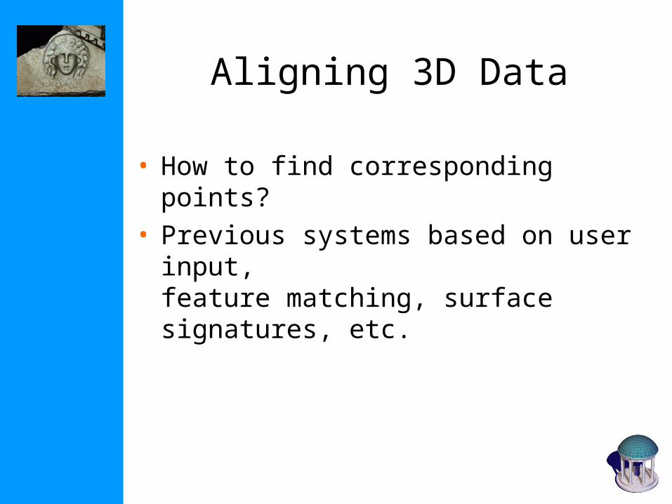
• How to find corresponding points?• Previous systems based on user
input,feature matching, surface signatures, etc.
Aligning 3D Data
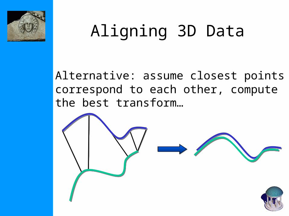
Alternative: assume closest points correspond to each other, compute the best transform…

Aligning 3D Data
… and iterate to find alignmentIterated Closest Points (ICP) [Besl & McKay
92]
Converges if starting position “close enough“

ICP Variants
• Classic ICP algorithm not real-time• To improve speed: examine stages of ICP and evaluate proposed variants
[Rusinkiewicz & Levoy, 3DIM 2001]
1.1. SelectingSelecting source points (from one or both meshes) source points (from one or both meshes)2.2. MatchingMatching to points in the other mesh to points in the other mesh3.3. WeightingWeighting the correspondences the correspondences4.4. RejectingRejecting certain (outlier) point pairs certain (outlier) point pairs5.5. Assigning an Assigning an error metricerror metric to the current transform to the current transform6.6. MinimizingMinimizing the error metric the error metric

ICP Variant – Point-to-Plane Error Metric
• Using point-to-plane distance instead of point-to-point lets flat regions slide along each other more easily [Chen & Medioni 91]

Finding Corresponding Points
• Finding closest point is most expensive stage of ICP• Brute force search – O(n)• Spatial data structure (e.g., k-d tree) – O(log n)• Voxel grid – O(1), but large constant, slow
preprocessing

Finding Corresponding Points
• For range images, simply project point [Blais 95]• Constant-time, fast• Does not require precomputing a spatial data
structure

High-Speed ICP Algorithm
• ICP algorithm with projection-based correspondences, point-to-plane matchingcan align meshes in a few tens of ms.(cf. over 1 sec. with closest-point)
[Rusinkiewicz & Levoy, 3DIM 2001]

3D Global Registration

3D Global registrationThe problem:• Given: n scans around an object• Goal: align them all• First attempt: ICP each scan to one
other

• Want method for distributing accumulated error among all scans
3D Global registration

Approach #1: Avoid the Problem
• In some cases have 1 scan that covers large part of surface (e.g., cylindrical scan)
• Align all other scans to this “anchor”• Disadvantage: not always practical to
obtain anchor scan

Approach #2: The Greedy Solution
• Align each new scan to all previous scans
• Disadvantages:• Order dependent• Doesn’t spread out error

Approach #3: Brute-Force Solution
• While not converged:• For each scan:
• For each point:– For every other scan
» Find closest point
• Minimize error w.r.t. transforms of all scans
• Disadvantage:• Solve (np)(np) matrix equation, where
n is number of scans and p is number of points per scan

Approach #3a: Slightly Less Brute-Force
• While not converged:• For each scan:
• For each point:– For every other scan
» Find closest point
• Minimize error w.r.t. transform of this scan
• Faster than previous method (matrices are pp)

Graph Methods
• Many globalreg algorithms create a graph of pairwise alignments between scans
Scan 1Scan 1Scan 1Scan 1 Scan 5Scan 5Scan 5Scan 5
Scan 4Scan 4Scan 4Scan 4
Scan 3Scan 3Scan 3Scan 3
Scan 2Scan 2Scan 2Scan 2 Scan 6Scan 6Scan 6Scan 6

Pulli’s Algorithm
• Perform pairwise ICPs, record sample (e.g. 200) of corresponding points
• For each scan, starting w. most connected• Align scan to existing set• While (change in error) > threshold
• Align each scan to others
• All alignments during globalreg phase use precomputed corresponding points

Sharp et al. Algorithm
• Perform pairwise ICPs, record only optimal rotation/translation for each
• Decompose alignment graph into cycles
• While (change in error) > tolerance• For each cycle:
• Spread out error equally among all scans in the cycle
• For each scan belonging to more than 1 cycle:
• Assign average transform to scan

Lu and Milios Algorithm
• Perform pairwise ICPs, record optimal rotation/translation and covariance for each
• Least squares simultaneous minimization of all errors (covariance-weighted)
• Requires linearization of rotations• Worse than the ICP case, since don’t
converge to (incremental rotation) = 0

Open Questions in Global Registration
• Best way to do correctly-weighted globalreg without linearizing rotations?
• How to prevent bias (if many scans in one area, few scans in another)?
• Robust outlier detection• For graph methods, pairwise ICP often
automated• One bad ICP can throw off the entire
model

Bad ICP in Globalreg
One bad ICP can throw off the entire model
Correct GlobalregCorrect Globalreg Globalreg Including Globalreg Including Bad ICPBad ICP

Huber’s Automatic Modeling System
• Start with unaligned cans• Generate candidate pairwise
alignments using spin images• Incrementally add scans, checking
consistency• ICP error in overlapping regions• Free space consistency• Occupied space consistency

Spin Images
• Johnson and Hebert• “Signature” that captures local
shape• Similar shapes similar spin
images

Computing Spin Images
• Start with a point on a 3D model• Find (averaged) surface normal at
that point• Define coordinate system centered
at this point, oriented according to surface normal and two (arbitrary) tangents
• Express other points (within some distance) in terms of the new coordinates

Computing Spin Images
• Compute histogram of locations of other points, in new coordinate system, ignoring rotation around normal:
n̂ p n̂ p
n̂p n̂p

Computing Spin Images

Spin Image Parameters
• Size of neighborhood• Determines whether local or global shape
is captured• Big neighborhood: more discriminatory
power• Small neighborhood: resistance to clutter
• Size of bins in histogram:• Big bins: less sensitive to noise• Small bins: captures more detail, less
storage

Using Spin Images for Alignment
Not robust

Verification – Overlap Distance
Views 1 and 2: 48%, 2.1 Views 1 and 2: 48%, 2.1 mmmm
Views 1 and 9: 15%, 3.1 mmViews 1 and 9: 15%, 3.1 mm

Verification – Visibility Consistency
consistentconsistentsurfacessurfaces
SS11 SS22
CC11 CC22
surfaces are closesurfaces are close
free spacefree spaceviolationviolation
SS11SS22
CC11CC22
SS22 blocks blocks SS11
occupied spaceoccupied spaceviolationviolation
SS11 SS22
CC11 CC22
SS11 is not observed is not observed

Automatically Modeling the Angel
top view
connectivity afterconnectivity afterlocal verificationlocal verification
horizontal slice
11
44
99
55
6688
1111
1212
1414
15151313
1010
22
33
77
11
44
99
55
6688
11111212
1414
15151313
1010
22
33
77
initial modelinitial model((bad matches in redbad matches in red))
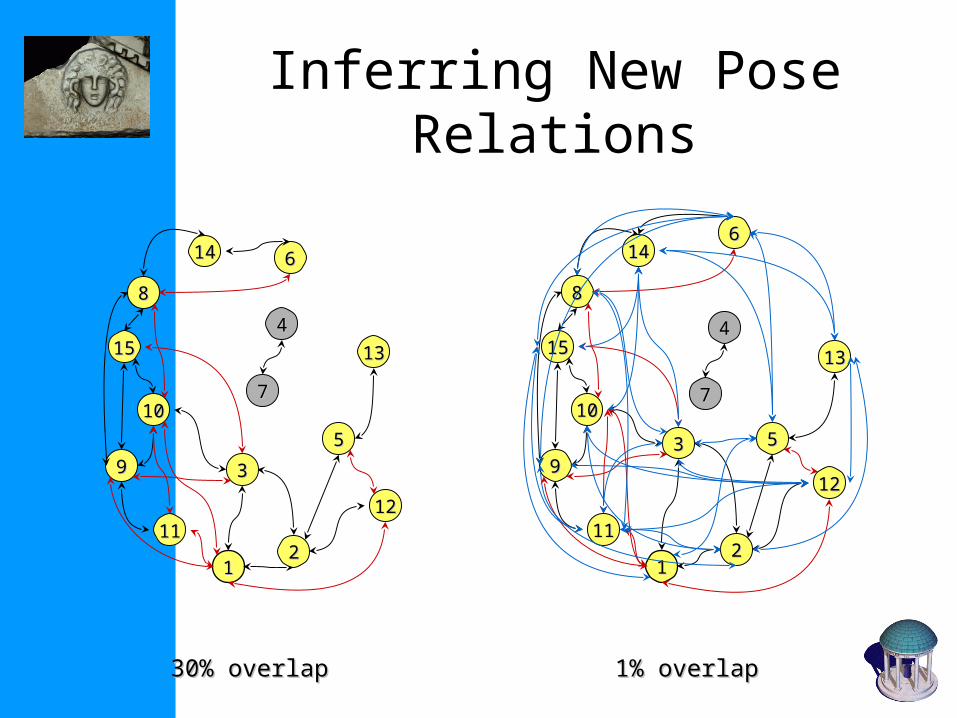
Inferring New Pose Relations
11
44
99
55
66
88
1111
1212
1414
15151313
1010
22
33
77
30% overlap30% overlap 1% overlap1% overlap
11
99
55
66
88
11111212
1414
1515 1313
1010
22
33
44
77

horizontal slice
The Final Angel Model
top view

Problems With Reconstruction from Point Clouds

Surface Reconstruction from Range Images
• Often an easier problem than reconstruction from arbitrary point clouds• Implicit information about adjacency,
connectivity• Roughly uniform spacing

Surface Reconstruction From Range Images
• First, construct surface from each range image
• Then, merge resulting surfaces• Obtain average surface in overlapping
regions• Control point density

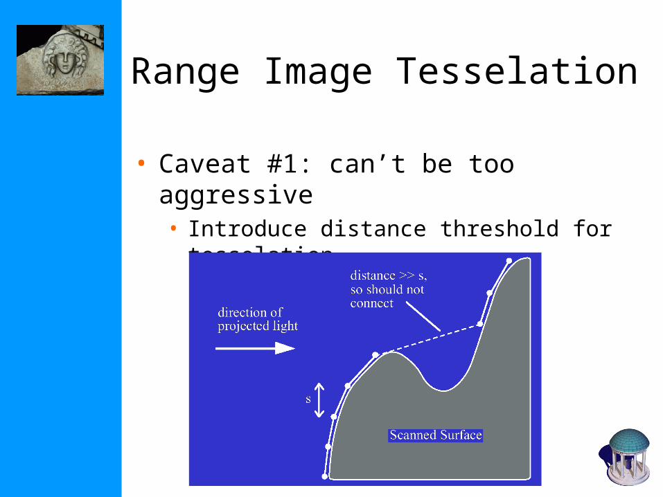
Range Image Tesselation
• Given a range image, connect up the neighbors

3D surface model
Depth image Triangle mesh Texture image
Textured 3DWireframe model
Range Image Tesselation
• Caveat #1: can’t be too aggressive• Introduce distance threshold for
tesselation

• Caveat #2: Which way to triangulate?
• Possible heuristics:• Shorter diagonal• Dihedral angle closer to 180• Maximize smallest angle in both triangles• Always the same way (best triangle
strips)
Range Image Tesselation

Scan Merging Using Zippering
• Turk & Levoy, 1994• Erode geometry in overlapping
areas• Stitch scans together along
seam• Re-introduce all data
• Weighted average

Zippering

Point Weighting
• Higher weights to points facing the camera• Favor higher sampling rates

Point Weighting
• Lower weights(tapering to 0)near boundaries• Smooth blends
between views

Volumetric Reconstruction
• Implicit function defined volumetrically
• Usually stored sampled on a 3D grid• Can be compressed (e.g., using RLE)• Another possibility: hierarchical data
structures
• Can extract isosurface (i.e., subset of space where implicit function = some constant)
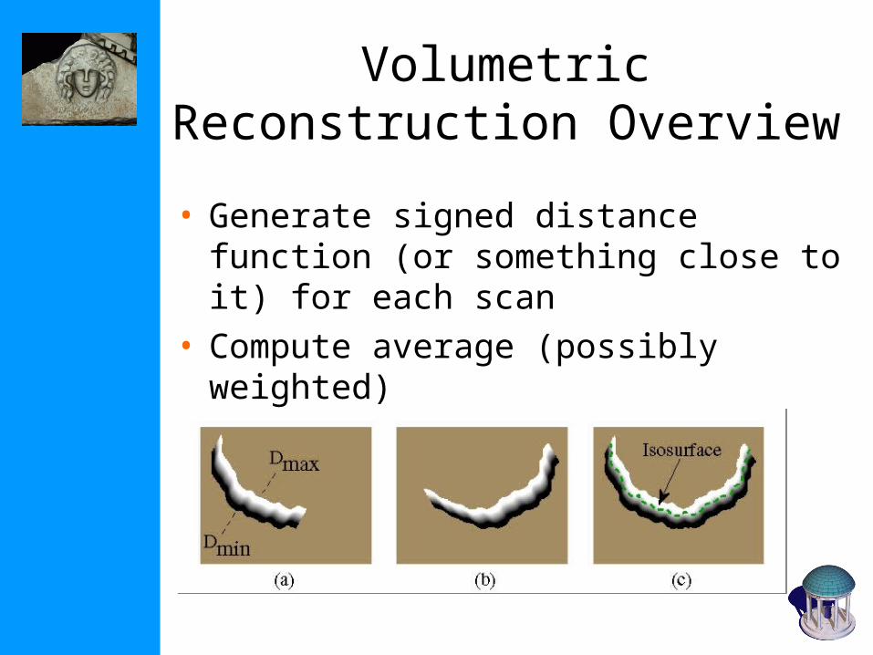
Volumetric Reconstruction Overview
• Generate signed distance function (or something close to it) for each scan
• Compute average (possibly weighted)
• Extract isosurface

Volumetric integration(Curless and Levoy, Siggraph´96)
sensor
range surfaces
volume
distance
depth
weight(~accuracy)
signed distanceto surface
surface1
surface2
combined estimate
• use voxel space• new surface as zero-crossing (find using marching cubes) • least-squares estimate (zero derivative=minimum)
Volumetric Reconstruction Benefits
• Always generates a manifold surface• Can control sampling density• Averaging of signed distance
functions corresponds to averaging the surfaces

Volumetric Reconstruction Drawbacks
• Represent a 3D entity rather than 2D• Running time• Storage
• Resampling step – bandlimits the function
• Generates consistent topology, but not always the topology you wanted
• Problems with very thin surfaces

From volume to mesh:Marching Cubes
First 2D, Marching Squares
“Marching Cubes: A High Resolution 3D Surface Construction Algorithm”,William E. Lorensen and Harvey E. Cline,Computer Graphics (Proceedings of SIGGRAPH '87), Vol. 21, No. 4, pp. 163-169.

From volume to mesh:Marching Cubes
“Marching Cubes: A High Resolution 3D Surface Construction Algorithm”,William E. Lorensen and Harvey E. Cline,Computer Graphics (Proceedings of SIGGRAPH '87), Vol. 21, No. 4, pp. 163-169.

From volume to mesh:Marching Cubes
Improvement
“Marching Cubes: A High Resolution 3D Surface Construction Algorithm”,William E. Lorensen and Harvey E. Cline,Computer Graphics (Proceedings of SIGGRAPH '87), Vol. 21, No. 4, pp. 163-169.

Multiple depth images Volumetric integration
Volumetric 3D integration

Next class: appearance modeling


