778 IEEE TRANSACTIONS ON ROBOTICS, VOL. 33, NO. 4, AUGUST 2017
Dynamic In-Hand Sliding ManipulationJian Shi, J. Zachary Woodruff, Student Member, IEEE, Paul B. Umbanhowar, and Kevin M. Lynch, Fellow, IEEE
Abstract—This paper presents a framework for planning themotion of an n-fingered robot hand to create an inertial load ona grasped object to achieve a desired in-grasp sliding motion. Themodel of the sliding dynamics is based on a soft-finger limit sur-face contact model at each fingertip. A motion planner is derivedto automatically solve for the finger motions for a given initial anddesired configuration of the object relative to the fingers. Iterativeplanning and execution are shown to reduce the errors that occurdue to the modeling and trajectory tracking errors. The frame-work is applied to the problem of regrasping a laminar objectheld in a pinch grasp. We propose a limited surface model of thecontact pressure distribution at each finger to predict the slidingdirections. Experimental validations are shown, including iterativeerror reduction and repeatability of the experiment.
Index Terms—Dexterous manipulation, dynamics, grasping,in-hand manipulation, manipulation planning.
I. INTRODUCTION
A. Background
MOST human, animal, and even robot manipulation tasksinvolve controlling motion of the object relative to the
manipulator, particularly in nonprehensile (graspless) manipu-lation modes such as pushing, rolling, pivoting, tipping, tapping,and kicking. Even in pick-carry-place manipulation, in whichthe carry portion of the task keeps the object stationary relativeto the hand, the pick and place phases typically involve the ob-ject sliding or rolling on the fingers as the hand achieves a firmgrasp or releases the object. Other examples of controlled rela-tive motion in grasping manipulation include finger gaiting, inwhich the fingers quasi-statically walk over the object to achievea regrasp, all the while maintaining a stable grasp, rolling theobject on the fingertips, and letting the object slide relative to thefingertips. Together we refer to these types of relative motion asin-hand manipulation.
We are studying in-hand manipulation by controlled slidingfor three purposes:
Manuscript received August 5, 2016; revised January 18, 2017; acceptedMarch 12, 2017. Date of publication April 27, 2017; date of current versionAugust 7, 2017. This paper was recommended for publication by Associate Ed-itor J. Piater and Editor A. Billard upon evaluation of the reviewers’ comments.This work was supported by the National Science Foundation under GrantIIS-0964665, Grant IIS-1527921, and Grant DGE-1324585. (Correspondingauthor: Jian Shi.)
J. Shi, J. Z. Woodruff, and P. B. Umbanhowar are with the Neuroscienceand Robotics Laboratory, Northwestern University, Evanston, IL 60208 USA(e-mail: [email protected]; [email protected];[email protected]).
K. M. Lynch is with the Neuroscience and Robotics Laboratory, North-western University, Evanston, IL 60208 USA, and is also with the North-western Institute on Complex Systems, Evanston, IL 60201 USA (e-mail:[email protected]).
Color versions of one or more of the figures in this paper are available onlineat http://ieeexplore.ieee.org.
Digital Object Identifier 10.1109/TRO.2017.2693391
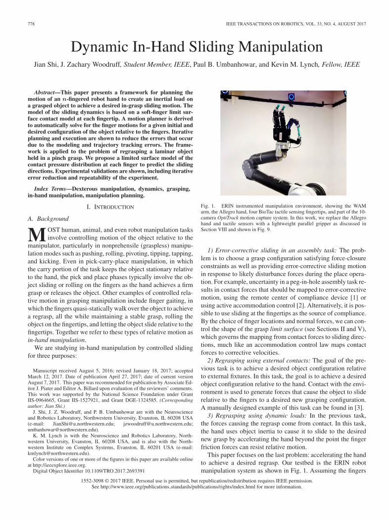
Fig. 1. ERIN instrumented manipulation environment, showing the WAMarm, the Allegro hand, four BioTac tactile sensing fingertips, and part of the 10-camera OptiTrack motion capture system. In this work, we replace the Allegrohand and tactile sensors with a lightweight parallel gripper as discussed inSection VIII and shown in Fig. 9.
1) Error-corrective sliding in an assembly task: The prob-lem is to choose a grasp configuration satisfying force-closureconstraints as well as providing error-corrective sliding motionin response to likely disturbance forces during the place opera-tion. For example, uncertainty in a peg-in-hole assembly task re-sults in contact forces that should be mapped to error-correctivemotion, using the remote center of compliance device [1] orusing active accommodation control [2]. Alternatively, it is pos-sible to use sliding at the fingertips as the source of compliance.By the choice of finger locations and normal forces, we can con-trol the shape of the grasp limit surface (see Sections II and V),which governs the mapping from contact forces to sliding direc-tions, much like an accommodation control law maps contactforces to corrective velocities.
2) Regrasping using external contacts: The goal of the pre-vious task is to achieve a desired object configuration relativeto external fixtures. In this task, the goal is to achieve a desiredobject configuration relative to the hand. Contact with the envi-ronment is used to generate forces that cause the object to sliderelative to the fingers to a desired new grasping configuration.A manually designed example of this task can be found in [3].
3) Regrasping using dynamic loads: In the previous task,the forces causing the regrasp come from contact. In this task,the hand uses object inertia to cause it to slide to the desirednew grasp by accelerating the hand beyond the point the fingerfriction forces can resist relative motion.
This paper focuses on the last problem: accelerating the handto achieve a desired regrasp. Our testbed is the ERIN robotmanipulation system as shown in Fig. 1. Assuming the fingers
SHI et al.: DYNAMIC IN-HAND SLIDING MANIPULATION 779
are compliantly mounted, and the initial grasp configuration ischosen, current research problems include:
1) given the state of the hand and object, the contact normalforces, and the acceleration of the hand, find the relativeacceleration of the object (forward dynamics);
2) given the state of the hand and object and the desiredrelative acceleration of the object, find appropriate handaccelerations and contact normal forces (inverse dynam-ics);
3) plan the hand motion (and possibly contact normal forces)to achieve a desired regrasp;
4) repeatedly plan and execute hand motions to iterativelyreduce grasp error;
5) use real-time feedback control of hand motion and fingernormal forces during sliding motion to achieve the desiredregrasp; and
6) estimate friction properties from observed hand and objectmotions, given the contact normal forces.
In this study, we use a simple, spring-actuated passive handin place of the Allegro hand and tactile sensors, and we studyitems (1)–(4) above. In particular, we focus on the case ofplanar motion, in which the laminar object moves with threedegrees of freedom (two translational and one rotational) andthe fingers contact the object on opposite sides that are parallelto the plane of motion. This paper extends our preliminarywork reported in [4].
B. Paper Outline
Section II reviews previous work on which this paper builds.In Section III, we solve problems (1)–(4) for a simple 1-DOF ex-ample, as a template for the more general case. In Section IV, wegeneralize the problem statement to an n-fingered grasp movingin a plane. In Section V, we discuss the limit surface model forfriction and derive expressions for the frictional wrench giventhe sliding velocity of an object in an n-fingered grasp con-sisting of patch contacts. In Section VI, we derive the slidingdynamics within the motion plane and outline a method to cal-culate the acceleration of the object relative to each finger giventhe accelerations of the fingers. In Section VII, we solve thefinger motion planning problem for a given n-fingered grasp toachieve a desired regrasp.
The material in Sections IV–VII solves the planar regraspproblem for general n-fingered grasps of an object with parallelfaces. The details of the finger normal forces and grasp limitsurface depend on the particular grasp configuration, however.In Section VIII, we derive the details of the grasp limit surfacefor a particular type of grasp, a two-fingered pinch grasp. InSection IX, we implement the motion planning algorithm forin-hand manipulation with a two-fingered pinch grasp, and weshow experimentally that iterative planning and execution canfurther reduce error in the final grasp configuration.
II. RELATED WORK
A. In-Hand Manipulation
There has been extensive work on kinematic in-hand manip-ulation where an object is moved relative to a finger without
breaking contact or sliding on the surface. This is sometimes re-ferred to as precision manipulation. Li et al. [5] and Yoshikawaand Nagai [6] used rigid, rolling finger contacts to calculategrasp stability and manipulability, and to develop controllersfor tracking a position trajectory while maintaining a desiredgrasp force. More recent related work by Rojas and Dollar [7]estimated the precision manipulation capabilities of arbitrarymanipulator/object configurations for use in autonomous ma-nipulation planning.
In-hand sliding manipulation can also be used to quicklyreposition an object in the hand. Traditional dexterous regraspmethods such as finger gaiting or “pick” and “place” may beslow or impossible given the number of fingers or the surround-ing environment. Brock [8] addressed the problem of controlledsliding by first generating a constraint state map that outlinesconstraints on a grasped object due to the contact types andforces. By varying the contact forces he achieved controlled slid-ing in desired directions for a grasped cylinder. Cole et al. [9]explored a dynamic coordinated control scheme to repositionobjects with controlled slip. Trinkle and Hunter [10] extendedthe dexterous manipulation planning problem to consider rollingand slipping contact modes. The hybrid planning problem wasfurther developed by Yashima et al. [11]. The space of reach-able object states can be further expanded by breaking con-tact with a single finger, moving it, and regrasping the objectwhile the remaining fingers maintain the object in force clo-sure. This in-hand regrasp technique is called finger gaiting[12]–[13].
Dynamic forces can also be used for in-hand manipulation.Furukawa et al. [14] demonstrated regrasping by tossing a foamcylinder up and catching it. Chavan-Dafle et al. [3] tested hand-coded regrasps that take advantage of external forces such asgravity, dynamic forces, and contact with the environment toregrasp objects using a simple manipulator. A more recent workby Chavan-Dafle et al. [15] explored in-hand manipulation ofan object by external contacts with the environment. With de-signed finger actions, motions of the object were simulated andvalidated experimentally with different shapes of contacts. Vinaet al. [16]–[17] showed that by using adaptive control with vi-sion and tactile feedback, monodirectional pivoting of an objectpinched by a pair of fingers can be achieved by changing thegripping forces. Kumar et al. [18] programmed a pneumati-cally actuated hand to learn in-hand manipulation skills usingmodel-based reinforcement learning. Sintov and Shapiro [19]developed an algorithm to swing up a rod by generating grippermotions, in which the contact point was modeled as a pivot jointthat can apply frictional torques. The method was validated insimulation. Hou et al. [20] studied dynamic planar pivoting ofa pinched object driven by the hand swing motion and contactnormal force control.
Arisumi et al. [21] explored casting manipulation where a ma-nipulator is thrown and its “free flight” trajectory is controlledin midair using tension forces on a tether. Similarly, dynamicin-hand sliding motions allow the manipulator to impart forceson the object during motion. This allows for feedback controland the ability to quickly regrasp the object at any point through-out the trajectory.
780 IEEE TRANSACTIONS ON ROBOTICS, VOL. 33, NO. 4, AUGUST 2017
B. Friction Modeling
Goyal et al. [22]–[24] describe the concept of a limit sur-face as a 2-D surface in a 3-D force–moment space. The limitsurface defines the maximum set of external wrenches that canbe resisted by the frictional forces due to the contact. Xydasand Kao [25] derived models of soft-finger contacts and theresulting limit surfaces. Recent work by Zhou et al. [26] pro-posed a fourth-order polynomial limit surface model for planarsliding and identified model parameters using simulation andexperimental data.
III. 1-DOF EXAMPLE
In this section, we address research topics (1)–(4) from theintroduction for a 1-DOF example with no gravity. This exampleserves as a template for the more general problem beginning inSection IV.
Consider an object that accelerates in the positive or negativedirection due to frictional contact with a single finger. Based on aCoulomb friction coefficient μ and a normal force fN , the fingercan provide a tangential force to the object of up to μfN beforesliding. We assume the object has unit mass, so the maximumobject acceleration is ao = μfN . We also assume the finger iscapable of a maximum acceleration af > ao . Additionally, wedefine a finger acceleration a greater than 0 but less than ao .The relationship between the accelerations can be written asaf > ao > a > 0.
Let qf (0) = qo(0) be the initial position of the finger andthe object w.r.t. the world frame W respectively, and let d(t) =qo(t) − qf (t) be the object position relative to the finger positionat time t. The problem is to choose a finger acceleration profileqf : [0, T ] → R that causes the object to slide relative to thefinger by dgoal at time T , i.e., d(T ) = qo(T ) − qf (T ) = dgoal asshown in Fig. 2. Without loss of generality, assume dgoal > 0.Similar reasoning applies for the case dgoal < 0.
A. Forward Dynamics
The forward dynamics problem is to determine the relativesliding acceleration d given a finger acceleration qf . If d �= 0,then d = sgn(d)ao − qf . If d = 0 and |qf | ≤ a0 , no sliding oc-curs (d = 0). If d = 0 and |qf | > a0 , then d = sgn(qf )a0 − qf .
B. Inverse Dynamics
The inverse problem is to determine the finger acceleration qfthat achieves a desired relative sliding acceleration d. If d �= 0,then qf = sgn(d)ao − d. If d = d = 0, no slip occurs so any|qf | ≤ ao is valid. If d = 0 and |d| > 0 (you are trying to initiateslip), then qf = sgn(d)a0 − d.
C. Motion Planning
We assume the finger and object are initially at rest andqf (0) = qo(0) = 0, and require that the finger’s net displace-ment and velocity after the motion are zero. To achieve thesliding regrasp while satisfying these constraints, we first ac-celerate the finger with qf = a for time T1 . We then apply the
Fig. 2. (Top) Configuration of the 1-DOF system. The red diamond showsthe center of mass (CM) of the object and the blue dot shows the contact pointof the finger. (Bottom) An example of in-hand sliding of the 1-DOF systemwith initial condition qf (0) = qo (0) = 0. The finger initially accelerates to theright, and then accelerates to the left causing the finger to slide on the object andachieve a desired position relative to the object CM dgoal. The correspondingacceleration, velocity, and position profiles are shown in Fig. 3.
maximum negative acceleration qf = −af for time T2 . Nextwe apply qf = a for time T3 + T4 = T34 . To achieve zero finaldisplacement and velocity for the finger, we choose T1 = T34and qf (T1) = −qf (T1 + T2).
The motion plan consists of three phases: an initial stick-ing phase of duration T1 , a sliding phase of duration T2 + T3 ,and a final sticking phase of duration T4 . During phase 1(0 ≤ t < T1), d is zero and |qf | ≤ ao so no relative motionoccurs. During the first part of phase 2 (T1 ≤ t < T1 + T2),the negative acceleration is sufficiently high that sliding occurs(qf < −ao ). During the second part of phase 2 (T1 + T2 ≤t < T1 + T2 + T3), the acceleration magnitude is decreased(|qf | ≤ ao ), but d �= 0 so sliding still occurs until d→ 0. Duringphase 3 (T1 + T2 + T3 ≤ t < T1 + T2 + T3 + T4), the object issticking and d = 0. Fig. 2 shows an example of in-hand slidingof the 1-DOF system. The full series of accelerations, resultingvelocities, and positions are shown in Fig. 3.
The total relative sliding distance dgoal is the integral betweenthe finger and object velocity curves in the sliding phase. Withgiven values of af , ao , a, and dgoal, we solve the following con-straints to find the durations T1 , T2 , T3 , and T4 :
2aT1 = af T2 (1)
ao(T2 + T3) = a(2T1 − T3) (2)
dgoal = 0.5(af − ao)(T 22 + T2T3) (3)
T4 = T1 − T3 . (4)
SHI et al.: DYNAMIC IN-HAND SLIDING MANIPULATION 781
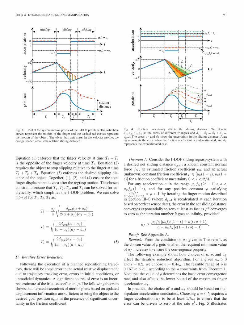
Fig. 3. Plot of the system motion profile of the 1-DOF problem. The solid bluecurves represent the motion of the finger and the dashed red curves representthe motion of the object. The object has unit mass. In the velocity profile, theorange shaded area is the relative sliding distance.
Equation (1) enforces that the finger velocity at time T1 + T2is the opposite of the finger velocity at time T1 . Equation (2)requires the object to stop slipping relative to the finger at timeT1 + T2 + T3 . Equation (3) enforces the desired slipping dis-tance of the object. Together, (1), (2), and (4) ensure the totalfinger displacement is zero after the regrasp motion. The chosenconstraints ensure that T1 , T2 , T3 , and T4 can be solved for an-alytically, which simplifies the 1-DOF problem. We can solve(1)–(3) for T1 , T2 , T3 as:
T1 =afa
√dgoal(a+ ao)
2(a+ af )(af − ao)
T2 =
√2dgoal(a+ ao)
(a+ af )(af − ao)
T3 =
√2dgoal(af − ao)
(a+ af )(a+ ao). (5)
D. Iterative Error Reduction
Following the execution of a planned repositioning trajec-tory, there will be some error in the actual relative displacementdue to trajectory tracking error, errors in initial conditions, orunmodeled dynamics. A significant source of error is an incor-rect estimate of the friction coefficient μ. The following theoremshows that iterated executions of motion plans based on updateddisplacement information are sufficient to bring the object to thedesired goal position dgoal in the presence of significant uncer-tainty in the friction coefficient.
Fig. 4. Friction uncertainty affects the sliding distance. We denoted1 , d2 , d3 , d4 as the areas of different triangles and d1 + d2 = d3 + d4 =dgoal. The areas d2 and d3 show the uncertainty in the sliding distance. Aread2 represents the error when the friction coefficient is underestimated, and d3represents the overestimated case.
Theorem 1: Consider the 1-DOF sliding regrasp system witha desired net sliding distance dgoal, a known constant normalforce fN , an estimated friction coefficient μ0 , and an actual(unknown) constant friction coefficient μ ∈ [μ0(1 − ε), μ0(1 +ε)] for a friction coefficient uncertainty 0 < ε < 2/3.
For any acceleration a in the range μ0fN (2ε− 1) < a <μ0fN (1 − ε), and for any positive constant ρ satisfying
μ0 fN εa+μ0 fN (1−ε) < ρ < 1, by iterating the finger motion describedin Section III-C (where dgoal is recalculated at each iterationbased on perfect sensor data), the error in the net sliding distanceconverges exponentially to zero at least as fast as ρk convergesto zero as the iteration number k goes to infinity, provided
Proof: See Appendix A.Remark: From the condition on af given in Theorem 1, as
the chosen value of ρ gets smaller, the required minimum valueof af increases to ensure the convergence property.
The following example shows how choices of a, ρ, and afaffect the iterative reduction algorithm. For a given ao > 0and ε = 0.2, we choose a = 0.4ao . The feasible range of ρ is0.167 < ρ < 1 according to the ρ constraints from Theorem 1.Note that the value of ρ determines the basic error convergencerate, and also affects the lower bound of the maximum fingeracceleration af .
In practice, the choice of ρ and af should be based on ma-nipulator acceleration constraints. Choosing ρ = 0.5 requires afinger acceleration af to be at least 1.7a0 to ensure that theerror can be driven to zero at the rate ρk . Fig. 5 illustrates
782 IEEE TRANSACTIONS ON ROBOTICS, VOL. 33, NO. 4, AUGUST 2017
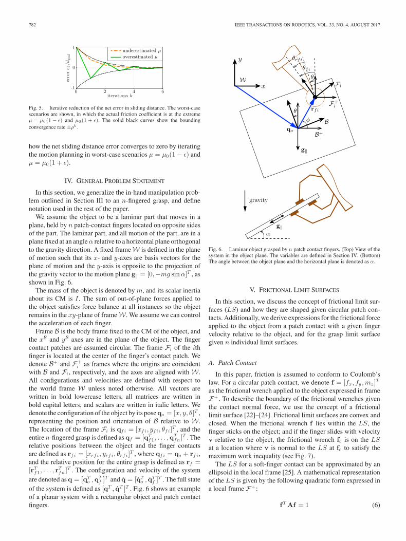
Fig. 5. Iterative reduction of the net error in sliding distance. The worst-casescenarios are shown, in which the actual friction coefficient is at the extremeμ = μ0 (1 − ε) and μ0 (1 + ε). The solid black curves show the boundingconvergence rate ±ρk .
how the net sliding distance error converges to zero by iteratingthe motion planning in worst-case scenarios μ = μ0(1 − ε) andμ = μ0(1 + ε).
IV. GENERAL PROBLEM STATEMENT
In this section, we generalize the in-hand manipulation prob-lem outlined in Section III to an n-fingered grasp, and definenotation used in the rest of the paper.
We assume the object to be a laminar part that moves in aplane, held by n patch-contact fingers located on opposite sidesof the part. The laminar part, and all motion of the part, are in aplane fixed at an angleα relative to a horizontal plane orthogonalto the gravity direction. A fixed frame W is defined in the planeof motion such that its x- and y-axes are basis vectors for theplane of motion and the y-axis is opposite to the projection ofthe gravity vector to the motion plane g‖ = [0,−mg sinα]T , asshown in Fig. 6.
The mass of the object is denoted by m, and its scalar inertiaabout its CM is I . The sum of out-of-plane forces applied tothe object satisfies force balance at all instances so the objectremains in the xy-plane of frame W . We assume we can controlthe acceleration of each finger.
Frame B is the body frame fixed to the CM of the object, andthe xB and yB axes are in the plane of the object. The fingercontact patches are assumed circular. The frame Fi of the ithfinger is located at the center of the finger’s contact patch. Wedenote B+ and F+
i as frames where the origins are coincidentwith B and Fi , respectively, and the axes are aligned with W .All configurations and velocities are defined with respect tothe world frame W unless noted otherwise. All vectors arewritten in bold lowercase letters, all matrices are written inbold capital letters, and scalars are written in italic letters. Wedenote the configuration of the object by its poseqo = [x, y, θ]T ,representing the position and orientation of B relative to W .The location of the frame Fi is qf i = [xf i, yf i , θf i ]T , and theentire n-fingered grasp is defined as qf = [qTf 1 , . . . ,q
Tf n ]T . The
relative positions between the object and the finger contactsare defined as rf i = [xrf i , yrf i , θrf i ]T , where qf i = qo + rf i ,and the relative position for the entire grasp is defined as rf =[rTf 1 , . . . , r
Tf n ]T . The configuration and velocity of the system
are denoted as q = [qTo ,qTf ]T and q = [qTo , q
Tf ]T . The full state
of the system is defined as [qT , qT ]T . Fig. 6 shows an exampleof a planar system with a rectangular object and patch contactfingers.
Fig. 6. Laminar object grasped by n patch contact fingers. (Top) View of thesystem in the object plane. The variables are defined in Section IV. (Bottom)The angle between the object plane and the horizontal plane is denoted as α.
V. FRICTIONAL LIMIT SURFACES
In this section, we discuss the concept of frictional limit sur-faces (LS) and how they are shaped given circular patch con-tacts. Additionally, we derive expressions for the frictional forceapplied to the object from a patch contact with a given fingervelocity relative to the object, and for the grasp limit surfacegiven n individual limit surfaces.
A. Patch Contact
In this paper, friction is assumed to conform to Coulomb’slaw. For a circular patch contact, we denote f = [fx, fy ,mz ]T
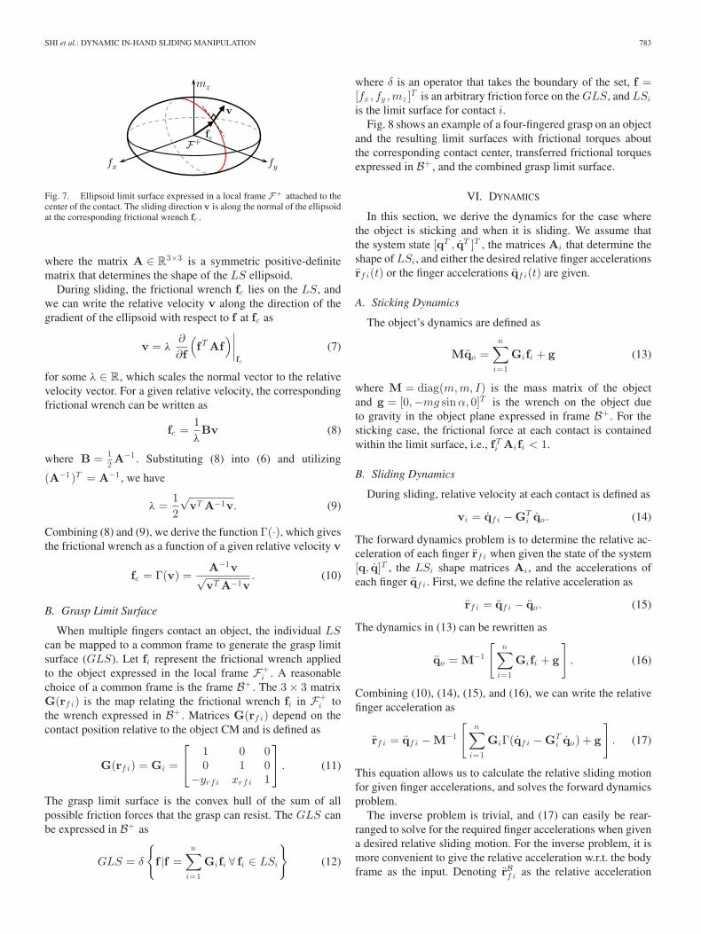
as the frictional wrench applied to the object expressed in frameF+ . To describe the boundary of the frictional wrenches giventhe contact normal force, we use the concept of a frictionallimit surface [22]–[24]. Frictional limit surfaces are convex andclosed. When the frictional wrench f lies within the LS, thefinger sticks on the object; and if the finger slides with velocityv relative to the object, the frictional wrench fc is on the LSat a location where v is normal to the LS at fc to satisfy themaximum work inequality (see Fig. 7).
The LS for a soft-finger contact can be approximated by anellipsoid in the local frame [25]. A mathematical representationof the LS is given by the following quadratic form expressed ina local frame F+ :
fT Af = 1 (6)
SHI et al.: DYNAMIC IN-HAND SLIDING MANIPULATION 783
Fig. 7. Ellipsoid limit surface expressed in a local frame F+ attached to thecenter of the contact. The sliding direction v is along the normal of the ellipsoidat the corresponding frictional wrench fc .
where the matrix A ∈ R3×3 is a symmetric positive-definitematrix that determines the shape of the LS ellipsoid.
During sliding, the frictional wrench fc lies on the LS, andwe can write the relative velocity v along the direction of thegradient of the ellipsoid with respect to f at fc as
v = λ∂
∂f
(fT Af
)∣∣∣∣fc
(7)
for some λ ∈ R, which scales the normal vector to the relativevelocity vector. For a given relative velocity, the correspondingfrictional wrench can be written as
fc =1λBv (8)
where B = 12 A−1 . Substituting (8) into (6) and utilizing
(A−1)T = A−1 , we have
λ =12
√vT A−1v. (9)
Combining (8) and (9), we derive the function Γ(·), which givesthe frictional wrench as a function of a given relative velocity v
fc = Γ(v) =A−1v√vT A−1v
. (10)
B. Grasp Limit Surface
When multiple fingers contact an object, the individual LScan be mapped to a common frame to generate the grasp limitsurface (GLS). Let fi represent the frictional wrench appliedto the object expressed in the local frame F+
i . A reasonablechoice of a common frame is the frame B+ . The 3 × 3 matrixG(rf i) is the map relating the frictional wrench fi in F+
i tothe wrench expressed in B+ . Matrices G(rf i) depend on thecontact position relative to the object CM and is defined as
G(rf i) = Gi =
⎡⎣ 1 0 0
0 1 0−yrf i xrf i 1
⎤⎦ . (11)
The grasp limit surface is the convex hull of the sum of allpossible friction forces that the grasp can resist. The GLS canbe expressed in B+ as
GLS = δ
{f |f =
n∑i=1
Gifi ∀ fi ∈ LSi
}(12)
where δ is an operator that takes the boundary of the set, f =[fx, fy ,mz ]T is an arbitrary friction force on theGLS, and LSiis the limit surface for contact i.
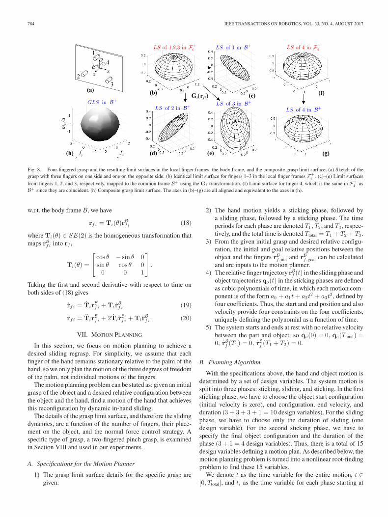
Fig. 8 shows an example of a four-fingered grasp on an objectand the resulting limit surfaces with frictional torques aboutthe corresponding contact center, transferred frictional torquesexpressed in B+ , and the combined grasp limit surface.
VI. DYNAMICS
In this section, we derive the dynamics for the case wherethe object is sticking and when it is sliding. We assume thatthe system state [qT , qT ]T , the matrices Ai that determine theshape of LSi , and either the desired relative finger accelerationsrf i(t) or the finger accelerations qf i(t) are given.
A. Sticking Dynamics
The object’s dynamics are defined as
Mqo =n∑i=1
Gifi + g (13)
where M = diag(m,m, I) is the mass matrix of the objectand g = [0,−mg sinα, 0]T is the wrench on the object dueto gravity in the object plane expressed in frame B+ . For thesticking case, the frictional force at each contact is containedwithin the limit surface, i.e., fTi Aifi < 1.
B. Sliding Dynamics
During sliding, relative velocity at each contact is defined as
vi = qf i − GTi qo . (14)
The forward dynamics problem is to determine the relative ac-celeration of each finger rf i when given the state of the system[q, q]T , the LSi shape matrices Ai , and the accelerations ofeach finger qf i . First, we define the relative acceleration as
rf i = qf i − qo . (15)
The dynamics in (13) can be rewritten as
qo = M−1
[n∑i=1
Gifi + g
]. (16)
Combining (10), (14), (15), and (16), we can write the relativefinger acceleration as
rf i = qf i − M−1
[n∑i=1
GiΓ(qf i − GTi qo) + g
]. (17)
This equation allows us to calculate the relative sliding motionfor given finger accelerations, and solves the forward dynamicsproblem.
The inverse problem is trivial, and (17) can easily be rear-ranged to solve for the required finger accelerations when givena desired relative sliding motion. For the inverse problem, it ismore convenient to give the relative acceleration w.r.t. the bodyframe as the input. Denoting rBf i as the relative acceleration
784 IEEE TRANSACTIONS ON ROBOTICS, VOL. 33, NO. 4, AUGUST 2017
Fig. 8. Four-fingered grasp and the resulting limit surfaces in the local finger frames, the body frame, and the composite grasp limit surface. (a) Sketch of thegrasp with three fingers on one side and one on the opposite side. (b) Identical limit surface for fingers 1–3 in the local finger frames F+
i . (c)–(e) Limit surfaces
from fingers 1, 2, and 3, respectively, mapped to the common frame B+ using the Gi transformation. (f) Limit surface for finger 4, which is the same in F+4 as
B+ since they are coincident. (h) Composite grasp limit surface. The axes in (b)–(g) are all aligned and equivalent to the axes in (h).
w.r.t. the body frame B, we have
rf i = Ti(θ)rBf i (18)
where Ti(θ) ∈ SE(2) is the homogeneous transformation thatmaps rBf i into rf i
Ti(θ) =
⎡⎣ cos θ − sin θ 0
sin θ cos θ 00 0 1
⎤⎦ .
Taking the first and second derivative with respect to time onboth sides of (18) gives
rf i = TirBf i + Ti rBf i (19)
rf i = TirBf i + 2Ti rBf i + Ti rBf i . (20)
VII. MOTION PLANNING
In this section, we focus on motion planning to achieve adesired sliding regrasp. For simplicity, we assume that eachfinger of the hand remains stationary relative to the palm of thehand, so we only plan the motion of the three degrees of freedomof the palm, not individual motions of the fingers.
The motion planning problem can be stated as: given an initialgrasp of the object and a desired relative configuration betweenthe object and the hand, find a motion of the hand that achievesthis reconfiguration by dynamic in-hand sliding.
The details of the grasp limit surface, and therefore the slidingdynamics, are a function of the number of fingers, their place-ment on the object, and the normal force control strategy. Aspecific type of grasp, a two-fingered pinch grasp, is examinedin Section VIII and used in our experiments.
A. Specifications for the Motion Planner
1) The grasp limit surface details for the specific grasp aregiven.
2) The hand motion yields a sticking phase, followed bya sliding phase, followed by a sticking phase. The timeperiods for each phase are denoted T1 , T2 , and T3 , respec-tively, and the total time is denoted Ttotal = T1 + T2 + T3 .
3) From the given initial grasp and desired relative configu-ration, the initial and goal relative positions between theobject and the fingers rBf ,init and rBf ,goal can be calculatedand are inputs to the motion planner.
4) The relative finger trajectory rBf (t) in the sliding phase andobject trajectories qo(t) in the sticking phases are definedas cubic polynomials of time, in which each motion com-ponent is of the form a0 + a1t+ a2t
2 + a3t3 , defined by
four coefficients. Thus, the start and end position and alsovelocity provide four constraints on the four coefficients,uniquely defining the polynomial as a function of time.
5) The system starts and ends at rest with no relative velocitybetween the part and object, so qo(0) = 0, qo(Ttotal) =0, rBf (T1) = 0, rBf (T1 + T2) = 0.
B. Planning Algorithm
With the specifications above, the hand and object motion isdetermined by a set of design variables. The system motion issplit into three phases: sticking, sliding, and sticking. In the firststicking phase, we have to choose the object start configuration(initial velocity is zero), end configuration, end velocity, andduration (3 + 3 + 3 + 1 = 10 design variables). For the slidingphase, we have to choose only the duration of sliding (onedesign variable). For the second sticking phase, we have tospecify the final object configuration and the duration of thephase (3 + 1 = 4 design variables). Thus, there is a total of 15design variables defining a motion plan. As described below, themotion planning problem is turned into a nonlinear root-findingproblem to find these 15 variables.
We denote t as the time variable for the entire motion, t ∈[0, Ttotal], and ti as the time variable for each phase starting at
SHI et al.: DYNAMIC IN-HAND SLIDING MANIPULATION 785
zero and ending at the duration of that phase, ti ∈ [0, Ti ], i =1, 2, 3. The details of the design variables and constraints oneach phase are given below.
1) First Sticking Phase: The design variables areqo(0),qo(T1), qo(T1), and T1 . The use of cubic polynomialsmeans there are no freedoms in the trajectory shapes once theboundary conditions are set. Therefore, qo(t1) is determinedwith a given set of the ten design variables. Note that becausethe initial relative position is not relevant to where the object isin the world frame, we can choose any initial position qo(0).The frictional wrench fi(t1) can be calculated by the stickingdynamics discussed in Section VI-A. Since there is no relativemotion in the sticking phase, the finger motions qf i(t1) are de-termined as long as qo(t1) and the relative positions rBf ,init aregiven.
The constraints that have to be satisfied are manipulator con-straints (including workspace, velocity, and acceleration limits)and that the frictional wrenches are always inside the limit sur-faces during the first sticking phase.
2) Sliding Phase: The design variable is T2 . In the slidingphase, the cubic polynomial defining the object motion relativeto the hand is fully specified by rBf ,init and rBf ,goal, which are given.The initial state of the hand is given by the design variablesqo(T1) and qo(T1) from the first sticking phase above. To findthe hand motion during this sliding phase, we first solve theinverse dynamics using the hand state at the beginning of thetrajectory, as well as rBf , to find the hand acceleration qf . Takinga small integration step, we get the next state of the hand, solvethe inverse dynamics again, etc., until we have numericallyconstructed the trajectory of the hand during the sliding phasebased on the initial state of the hand and the prespecified relativeobject motion during sliding.
The constraints that have to be satisfied in the sliding phaseare manipulator constraints.
3) Second Sticking Phase: The design variables are qo(Ttotal)and T3 . Similar to the first sticking phase, the hand motionqf i(t3) and object motion qo(t3) are determined by the speci-fied final conditions and the initial conditions q(T1 + T2) andq(T1 + T2) from the final state of the sliding phase.
The constraints that have to be satisfied are manipulator con-straints and that the frictional wrenches are always inside thelimit surfaces during the second sticking phase.
This is a multidimensional root-finding problem with con-straints, and we use MATLAB’s fmincon SQP solver to solveit. An initial guess of the design variables is automatically gen-erated based on heuristics encoding our knowledge of the task.
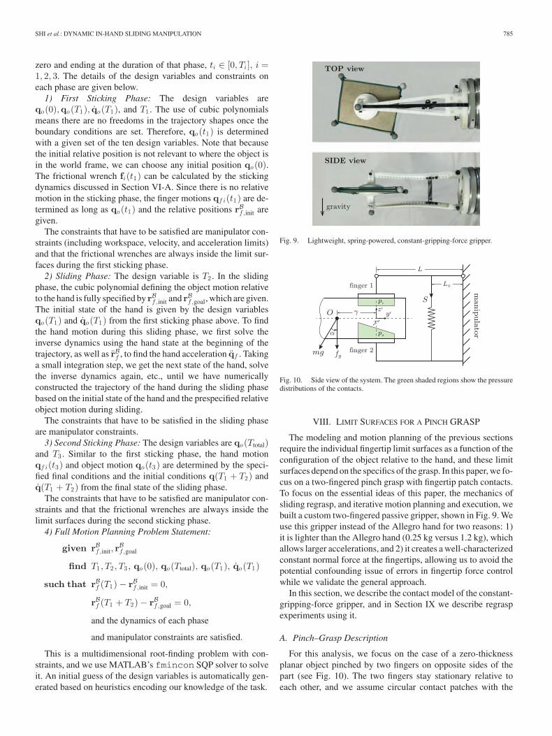
Fig. 10. Side view of the system. The green shaded regions show the pressuredistributions of the contacts.
VIII. LIMIT SURFACES FOR A PINCH GRASP
The modeling and motion planning of the previous sectionsrequire the individual fingertip limit surfaces as a function of theconfiguration of the object relative to the hand, and these limitsurfaces depend on the specifics of the grasp. In this paper, we fo-cus on a two-fingered pinch grasp with fingertip patch contacts.To focus on the essential ideas of this paper, the mechanics ofsliding regrasp, and iterative motion planning and execution, webuilt a custom two-fingered passive gripper, shown in Fig. 9. Weuse this gripper instead of the Allegro hand for two reasons: 1)it is lighter than the Allegro hand (0.25 kg versus 1.2 kg), whichallows larger accelerations, and 2) it creates a well-characterizedconstant normal force at the fingertips, allowing us to avoid thepotential confounding issue of errors in fingertip force controlwhile we validate the general approach.
In this section, we describe the contact model of the constant-gripping-force gripper, and in Section IX we describe regraspexperiments using it.
A. Pinch–Grasp Description
For this analysis, we focus on the case of a zero-thicknessplanar object pinched by two fingers on opposite sides of thepart (see Fig. 10). The two fingers stay stationary relative toeach other, and we assume circular contact patches with the
786 IEEE TRANSACTIONS ON ROBOTICS, VOL. 33, NO. 4, AUGUST 2017
same fixed radius a. The plane in which the object and themanipulator move is tilted by angle α from the horizontal planeas shown in Fig. 6. We denote fg = −mg cosα as the gravityforce acting on the object in the out-of-plane direction.
Finger 1, on the top of the object, is connected to the manip-ulator by two hinges and an arm of length L. Finger 2, on thebottom of the object, is connected to the manipulator through anarm fixed to the manipulator with the same length L. The twohinges keep the two flat circular fingers parallel to each otherand in full contact with the object. The distance from the hingesto the contact of finger 1 is assumed to be zero. The spring islocated LS away from the manipulator and the spring force isdenoted S. This model allows us to control the normal forces atthe fingers by the spring stiffness (another model could be forcecontrol of the manipulator in the normal direction and motioncontrol in the two linear tangent directions and rotation aboutthe contact normal).
B. Fingertip Limit Surfaces
We first note four important features of the two-fingered pinchgrasp:
1) Collocated Point Fingers Cannot Hold the Object: Re-membering that the laminar object is modeled in the limitof zero thickness, the contact point of each finger wouldbe at the same point. Therefore, contact forces from thetwo collocated fingertips always make zero moment aboutthe contact point, and they cannot balance the moment dueto gravity. This issue can be addressed by having contactpatches instead of point contacts.
2) Pressure Distribution at a Contact Patch is GenerallyUnknowable: If the object and fingertip are modeled asrigid bodies, then the pressure as a function of the locationon a continuous contact patch will be indeterminate. Ourapproach is to use the simplest possible model of thepressure distribution that is physically consistent, and toaccount for any unknowable modeling errors by iterativeregrasping.
3) Simplest Pressure Distribution, Uniform Pressure, isPhysically Inconsistent: If both contact patches have auniform pressure distribution, then the two design vari-ables available (the pressure at each patch) are insufficientto provide force–moment balance of the object in gravity.
4) Lowest Order Physically Consistent Pressure Distribu-tion Model is Uniform Pressure on Finger 1 and LinearlyVarying Pressure on Finger 2: The uniform pressure onfinger 1 assures that the total normal force passes throughthe rotational joint above the finger. The linearly vary-ing pressure distribution on finger 2 provides the extravariable needed to solve uniquely for the pressure distri-butions while assuring that the object remains in the planeof motion.
Fig. 10 illustrates the two contact pressure distributions,viewed from the side. The pressure p1 is constant over the con-tact patch, modeled as a disk of radius a. The pressure p2 isalso defined over a disk of radius a. Defining a y′ axis as theaxis from the center of mass of the object to the center of the
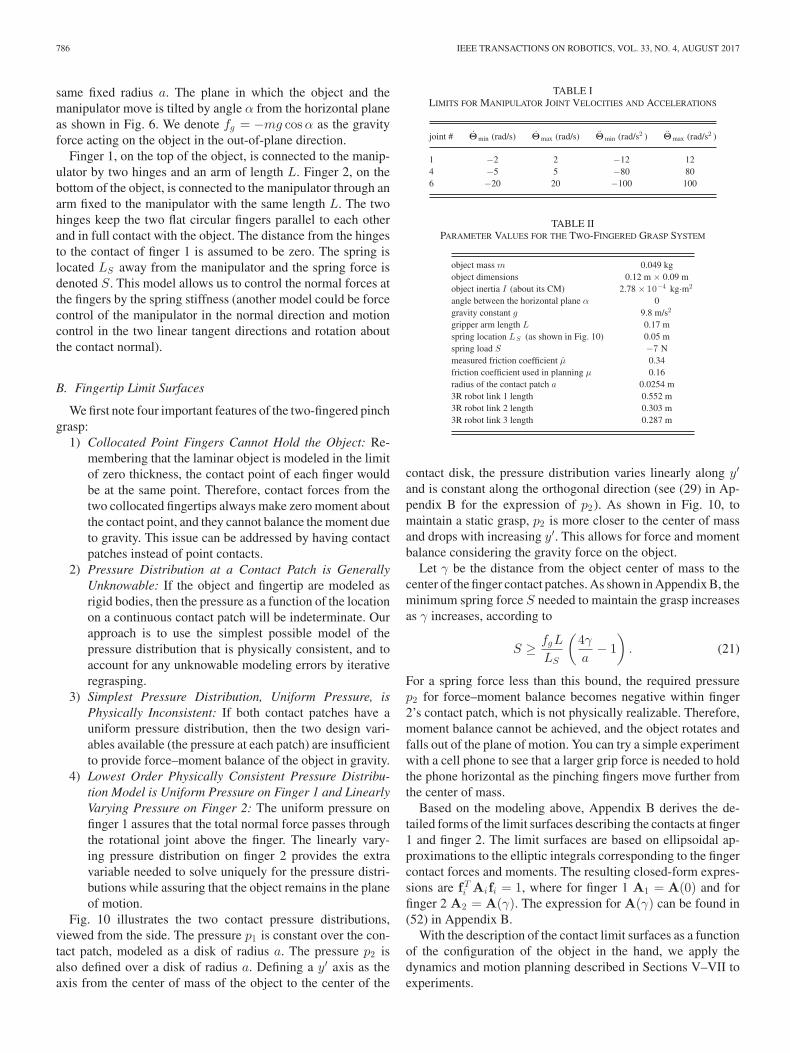
TABLE ILIMITS FOR MANIPULATOR JOINT VELOCITIES AND ACCELERATIONS
TABLE IIPARAMETER VALUES FOR THE TWO-FINGERED GRASP SYSTEM
object mass m 0.049 kgobject dimensions 0.12 m × 0.09 mobject inertia I (about its CM) 2.78 × 10⁻⁴ kg·m2
angle between the horizontal plane α 0gravity constant g 9.8 m/s2
gripper arm length L 0.17 mspring location LS (as shown in Fig. 10) 0.05 mspring load S −7 Nmeasured friction coefficient μ 0.34friction coefficient used in planning μ 0.16radius of the contact patch a 0.0254 m3R robot link 1 length 0.552 m3R robot link 2 length 0.303 m3R robot link 3 length 0.287 m
contact disk, the pressure distribution varies linearly along y′
and is constant along the orthogonal direction (see (29) in Ap-pendix B for the expression of p2). As shown in Fig. 10, tomaintain a static grasp, p2 is more closer to the center of massand drops with increasing y′. This allows for force and momentbalance considering the gravity force on the object.
Let γ be the distance from the object center of mass to thecenter of the finger contact patches. As shown in Appendix B, theminimum spring force S needed to maintain the grasp increasesas γ increases, according to
S ≥ fgL
LS
(4γa
− 1). (21)
For a spring force less than this bound, the required pressurep2 for force–moment balance becomes negative within finger2’s contact patch, which is not physically realizable. Therefore,moment balance cannot be achieved, and the object rotates andfalls out of the plane of motion. You can try a simple experimentwith a cell phone to see that a larger grip force is needed to holdthe phone horizontal as the pinching fingers move further fromthe center of mass.
Based on the modeling above, Appendix B derives the de-tailed forms of the limit surfaces describing the contacts at finger1 and finger 2. The limit surfaces are based on ellipsoidal ap-proximations to the elliptic integrals corresponding to the fingercontact forces and moments. The resulting closed-form expres-sions are fTi Aifi = 1, where for finger 1 A1 = A(0) and forfinger 2 A2 = A(γ). The expression for A(γ) can be found in(52) in Appendix B.
With the description of the contact limit surfaces as a functionof the configuration of the object in the hand, we apply thedynamics and motion planning described in Sections V–VII toexperiments.
SHI et al.: DYNAMIC IN-HAND SLIDING MANIPULATION 787
Fig. 11. Repositioning example: showing trajectories found by the motion planner. The plot on the left shows the entire motion with a time interval betweenframes of 60 ms. Plots on the right show the initial and final configurations, and give more details of motion during the sliding phase. Solid gray curves are theobject CM trajectories, red dots represent the finger contacts, and the brown lines represent the finger orientation. Thick black arrows show the directions of theobject motion. Thick black curves show the sliding regions. Thin red and green arrows are the x and y directions of the body frame B.
Fig. 12. Repositioning example: showing the trajectories of the object (red dashed curves) and the finger (blue solid curves) found by the motion planner toreposition an object. Green shaded regions show the planned sliding phase. (Left) Finger contact center trajectories qf and object CM trajectories qo . Initialrelative position error is shown as the space between the dashed red line and the blue line, which is reduced to zero after the sliding motion. (Middle) Fingervelocities qf and object contact points velocities (points on the object that are coincident with the contact center) GT qo are shown to demonstrate relativevelocities at the contact. (Right) Finger accelerations qf and object contact point accelerations d
dt (GT qo ) demonstrate relative accelerations at the contact.
IX. EXPERIMENT
We tested the motion planner discussed in Section VII with apinch–grasp introduced in Section VIII using the ERIN systemdescribed in Section I-A.
We used the lightweight passive gripper rather than the Al-legro hand for the higher achievable accelerations and bettercontact force characterization as discussed in the beginning ofSection VIII. We used three joints of the 7-DOF WAM arm(joints 1, 4, and 6) while keeping the other joints fixed to em-ulate a 3R planar arm. Manipulator workspace, velocity, andacceleration constraints in the root-finding problem were basedon joint, velocity, and motor properties given by the manufac-turer as well as conservative estimates of the inertia matrix. Thevalues of manipulator velocity and acceleration constraints areshown in Table I.
Given initial and goal relative configurations, the motion plan-ner plans the hand trajectory and solves the joint trajectoriesusing inverse kinematics. The planned joint trajectories weregenerated offline, and real-time control was used to follow thetrajectories specified by the planner. The motion control loopused encoder feedback and ran at 500 Hz on a Linux PC withan Intel Core i7-4770 CPU and 16 GB RAM. Motion was in ahorizontal plane (α = 0) to achieve more isotropic control au-thority than would be the case in a vertical plane. The valuesof the constants used in modeling and planning are summarizedin Table II.
A. One-Shot Planning and Execution
Before planning, the initial relative position rBf ,init was mea-sured by the vision system. With the goal relative position rBf ,goal
788 IEEE TRANSACTIONS ON ROBOTICS, VOL. 33, NO. 4, AUGUST 2017
Fig. 13. Repositioning example: blue curves showing the planned joint positions, velocities, and accelerations of the manipulator calculated from the fingertrajectories shown in Fig. 12 by solving inverse kinematics. The green dashed lines are the joint velocity and acceleration limits corresponding to the values inTable I. Joint position limits are not shown since the trajectories are far from the limits.
Fig. 14. Experiment result of one-shot planning showing the relative positionchanges versus time. Red dashed curves show the reference relative positionrBf trajectories. Blue curves represent the actual relative position trajectories.Green shaded regions indicate the planned sliding phase.
Fig. 15. Experiment result of one-shot planning, showing the finger contactcenter trajectories. Green shaded regions indicate the planned sliding phase.The mean absolute tracking errors are [1.02 mm, 2.56 mm, 0.296 ◦]T , and thestandard deviations are [1.04 mm, 2.75 mm, 0.27 ◦]T .
given by the user, the motion planner calculated the motion of therobot to realize the repositioning satisfying all the constraints.
Figs. 11 and 12 show the motion planning result of a slid-ing regrasp example. The initial relative position was measuredas rBf ,init = [−0.011 m,−0.022 m, 164◦]T , and the goal relative
position was given as rBf ,goal = [0, 0, 180◦]T . Fig. 13 shows theplanned joint trajectories of the 3R robot, which were calcu-lated from the inverse kinematics applied to the finger positiontrajectories in Fig. 12. The planned time periods for each phasewere T1 = 0.64 s, T2 = 0.29 s, and T3 = 1.33 s.
The planned motions were tested experimentally. The WAMarm followed the preplanned joint trajectories using a PID-based joint position controller. The object poses were obtainedfrom the vision system. To prevent overshoot during the slid-ing motion, we chose an underestimated friction coefficient inthe motion planner. Experimental results of relative positionchange are shown in Fig. 14. Finger position tracking results areshown in Fig. 15, where the finger poses were calculated fromthe recorded joint angles and the forward kinematics of thesystem.
During the implementation, the finger moved relative to theobject along the desired direction and ended up with some un-dershoot errors, which were more apparent in the y direction.One reason for this undershoot is the intentionally underesti-mated friction coefficient in the motion planner. Another reasonis the trajectory tracking error is larger in the y direction asshown in Fig. 15. Since there is more error in the y directionfrom the initial configuration, the planned motion has higher ac-celerations in this direction, which increases the tracking error.The final relative position errors could also have been causedby modeling errors and uncertainties in measuring the initialrelative positions.
B. Iterative Planning and Execution
This section reports the results of iterative planning and exe-cution for 3-DOF planar regrasping. Unlike the idealized 1-DOFexample in Section III, we have no theoretical convergence re-sults for iterative in-hand regrasping for the 3-DOF case and allpossible sources of error. The motivation for iterative regrasping(essentially discrete-time one-step deadbeat feedback control)is the same, however.
In each experiment, we tested three iterations of motion plan-ning and execution with the same goal. In each iteration, the
SHI et al.: DYNAMIC IN-HAND SLIDING MANIPULATION 789
Fig. 16. Experimental results of iterative planning and execution for one experiment consisting of three iterations. The plots show the planned and actual relativeconfigurations rBf (t). Each color represents one iteration. Triangles and circles show the initial and final points of each trajectory. The dashed lines are the plannedtrajectories and the solid curves shows the experimental results. Plots on the left and right show the same result from different viewpoints.
Fig. 17. Iterative planning experiment corresponding to Fig. 16. Total times for iterations 0, 1, and 2 are 2.26 s, 1.6 s, and 1.95 s, respectively. Time intervalsbetween snapshots were manually chosen to show the motion of the system. A video of this experiment is shown in the attached media.
initial state was measured from the last state of the previousiteration. The robot trajectories were planned automatically bythe motion planner based on the initial state and goal state. Then,the robot followed the planned trajectories.
Results of the iterative planning are shown in Figs. 16 and17. The first iteration corresponds to the example given inSection IX-A. After each iteration, the relative position wascloser to the goal configuration. Once the object is near thegoal state, additional iterations did not decrease the error. Incases where the error was close to the mean vision error of thevision system (∼0.5 mm), additional iterations could actuallyintroduce more error.
C. Repeatability
To test the repeatability of the repositioning experiment, weran the previous three-iteration experiment ten times, makinga total of 30 motion plans and executions. At the beginningof each three-iteration trial, the object was manually placed at
approximately the same initial configuration. Fig. 18 shows aboxplot of the relative position changes. Fig. 19 shows a boxplotof the planning time. Further iterations produce no statisticallysignificant improvement (or worsening) of the grasp.
Sources of error in achieving planned regrasps include vi-sion errors (as mentioned above), error in following the plannedrobot trajectory, and contact modeling errors (e.g., the Coulombfriction approximation and the contact pressure distribution ap-proximations). The mean absolute robot trajectory tracking er-rors were [1.2 mm, 2.6 mm, 0.35 ◦]T , with standard deviations[0.91 mm, 2.6 mm, 0.22 ◦]T , respectively. Errors induced by theassumed form of the contact pressure distributions are likelyless meaningful for n-fingered grasps than for our 2-fingeredgrasp, because the distances between the finger contacts playa larger role in determining the shape of the grasp limit sur-face than the detailed pressure distribution at single fingers.While our finger/object contacts approximately obeyed a dryCoulomb friction model, other finger/object contacts, particu-
790 IEEE TRANSACTIONS ON ROBOTICS, VOL. 33, NO. 4, AUGUST 2017
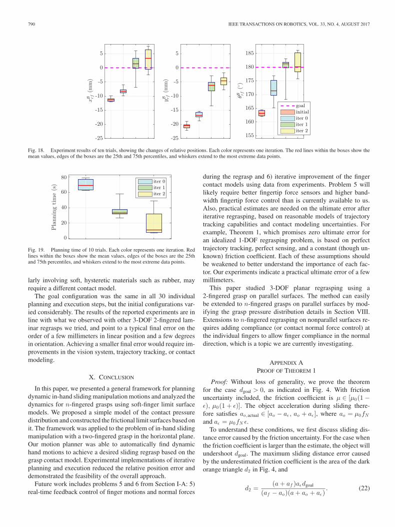
Fig. 18. Experiment results of ten trials, showing the changes of relative positions. Each color represents one iteration. The red lines within the boxes show themean values, edges of the boxes are the 25th and 75th percentiles, and whiskers extend to the most extreme data points.
Fig. 19. Planning time of 10 trials. Each color represents one iteration. Redlines within the boxes show the mean values, edges of the boxes are the 25thand 75th percentiles, and whiskers extend to the most extreme data points.
larly involving soft, hysteretic materials such as rubber, mayrequire a different contact model.
The goal configuration was the same in all 30 individualplanning and execution steps, but the initial configurations var-ied considerably. The results of the reported experiments are inline with what we observed with other 3-DOF 2-fingered lam-inar regrasps we tried, and point to a typical final error on theorder of a few millimeters in linear position and a few degreesin orientation. Achieving a smaller final error would require im-provements in the vision system, trajectory tracking, or contactmodeling.
X. CONCLUSION
In this paper, we presented a general framework for planningdynamic in-hand sliding manipulation motions and analyzed thedynamics for n-fingered grasps using soft-finger limit surfacemodels. We proposed a simple model of the contact pressuredistribution and constructed the frictional limit surfaces based onit. The framework was applied to the problem of in-hand slidingmanipulation with a two-fingered grasp in the horizontal plane.Our motion planner was able to automatically find dynamichand motions to achieve a desired sliding regrasp based on thegrasp contact model. Experimental implementations of iterativeplanning and execution reduced the relative position error anddemonstrated the feasibility of the overall approach.
Future work includes problems 5 and 6 from Section I-A: 5)real-time feedback control of finger motions and normal forces
during the regrasp and 6) iterative improvement of the fingercontact models using data from experiments. Problem 5 willlikely require better fingertip force sensors and higher band-width fingertip force control than is currently available to us.Also, practical estimates are needed on the ultimate error afteriterative regrasping, based on reasonable models of trajectorytracking capabilities and contact modeling uncertainties. Forexample, Theorem 1, which promises zero ultimate error foran idealized 1-DOF regrasping problem, is based on perfecttrajectory tracking, perfect sensing, and a constant (though un-known) friction coefficient. Each of these assumptions shouldbe weakened to better understand the importance of each fac-tor. Our experiments indicate a practical ultimate error of a fewmillimeters.
This paper studied 3-DOF planar regrasping using a2-fingered grasp on parallel surfaces. The method can easilybe extended to n-fingered grasps on parallel surfaces by mod-ifying the grasp pressure distribution details in Section VIII.Extensions to n-fingered regrasping on nonparallel surfaces re-quires adding compliance (or contact normal force control) atthe individual fingers to allow finger compliance in the normaldirection, which is a topic we are currently investigating.
APPENDIX APROOF OF THEOREM 1
Proof: Without loss of generality, we prove the theoremfor the case dgoal > 0, as indicated in Fig. 4. With frictionuncertainty included, the friction coefficient is μ ∈ [μ0(1 −ε), μ0(1 + ε)]. The object acceleration during sliding there-fore satisfies ao,actual ∈ [ao − aε, ao + aε ], where ao = μ0fNand aε = μ0fN ε.
To understand these conditions, we first discuss sliding dis-tance error caused by the friction uncertainty. For the case whenthe friction coefficient is larger than the estimate, the object willundershoot dgoal. The maximum sliding distance error causedby the underestimated friction coefficient is the area of the darkorange triangle d2 in Fig. 4, and
d2 =(a+ af )aεdgoal
(af − ao)(a+ ao + aε). (22)
SHI et al.: DYNAMIC IN-HAND SLIDING MANIPULATION 791
For the case where the actual friction coefficient is smallerthan the estimate, the object will slide more than dgoal. Themaximum sliding distance error is the area of the dark greentriangle d3 in Fig. 4, which can be expressed as
d3 =(a+ af )aεdgoal
(af − ao)(a+ ao − aε). (23)
From (22) and (23), the maximum sliding distance errorssatisfy d2 < d3 for any af > ao regardless of what af is chosen.Therefore, we focus on the conditions on d3 to ensure that thesliding distance errors decrease within the given rate.
From (23), when af > ao , and with given ao and aε , asaf increases to infinity d3 converges to its minimum value ofaε dgoal
a+ao−aε . Although it initially seems counterintuitive, increasingthe finger acceleration af decreases the overshoot error becausethe phase durations become smaller [see (5)]. To prevent theobject from sliding too far, the condition d3 < dgoal should beensured. Therefore, we have a lower bound for a:
aεa+ ao − aε
< 1 ⇒ a > μ0fN (2ε− 1).
An upper bound on a ensures that the object sticks in the be-ginning and end modes when the friction is overestimated, andis expressed by a < μ0fN (1 − ε). To ensure a feasible a exists,the upper and lower bounds of a should satisfy
μ0fN (2ε− 1) < μ0fN (1 − ε) ⇒ ε < 2/3.
Note that the decrease of the net sliding error from one iter-ation to the next is never better than aε
a+ao−aε = μ0 fN εa+μ0 fN (1−ε) .
This gives the lower bound on the feasible convergence rate ρ.The range of the actual sliding distance can be written as
dactual ∈ [dgoal − d2 , dgoal + d3 ], and the error in sliding distanceas e = dgoal − dactual ∈ [d2 ,−d3 ].
At each iteration, the error ek from the previous iterationbecomes new (dgoal)k and is used to replan a sliding motion:
To have the error in the net sliding distance converge to zeroat least as fast as ρk , we need to choose a maximum fingeracceleration af such that ek ≤ ρ(dgoal)k . For the case of anoverestimated friction coefficient, (3) and (22) show that whenaf ≥ μ0 fN [μ0 fN (ε−1)ρ−a(ε+ρ)]
μ0 fN (ερ−ρ+ε)−aρ we have
|(d2)k ||(dgoal)k | ≤
ao + a− aεao + a+ aε
ρ < ρ. (25)
Similarly for the case of an underestimated friction coefficient,(3) and (23) show that when af ≥ μ0 fN [μ0 fN (ε−1)ρ−a(ε+ρ)]
μ0 fN (ερ−ρ+ε)−aρ wehave
|(d3)k ||(dgoal)k | ≤ ρ. (26)
From (22) and (23), we have d2 < d3 for any af > ao . There-fore, we only need to satisfy the af constraint that leads to (25),
which yields af ≥ μ0 fN [μ0 fN (ε−1)ρ−a(ε+ρ)]μ0 fN (ερ−ρ+ε)−aρ .
Combining (24)–(26) gives∣∣∣ (dgoal)k + 1
(dgoal)k
∣∣∣ < ρ, which demon-
strates that |(dgoal)k | converges exponentially to zero as thenumber of iterations k increases. �
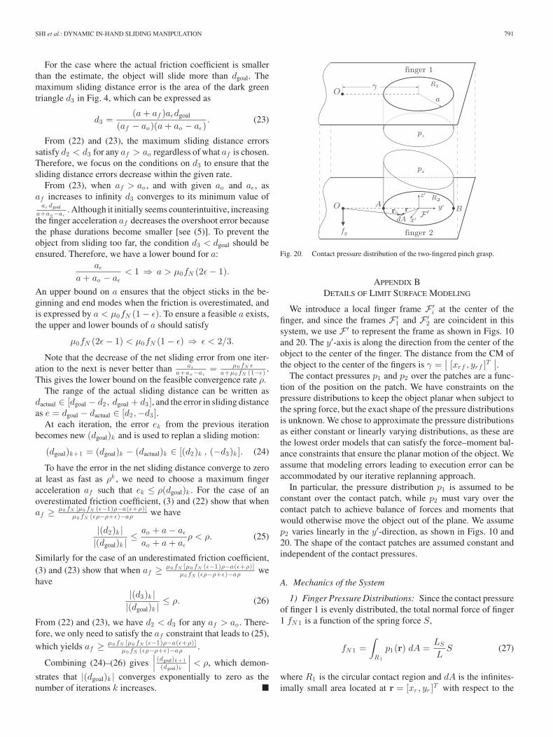
Fig. 20. Contact pressure distribution of the two-fingered pinch grasp.
APPENDIX BDETAILS OF LIMIT SURFACE MODELING
We introduce a local finger frame F′i at the center of the
finger, and since the frames F′1 and F′
2 are coincident in thissystem, we use F′ to represent the frame as shown in Figs. 10and 20. The y′-axis is along the direction from the center of theobject to the center of the finger. The distance from the CM ofthe object to the center of the fingers is γ =
∣∣ [xrf , yrf ]T∣∣.
The contact pressures p1 and p2 over the patches are a func-tion of the position on the patch. We have constraints on thepressure distributions to keep the object planar when subject tothe spring force, but the exact shape of the pressure distributionsis unknown. We chose to approximate the pressure distributionsas either constant or linearly varying distributions, as these arethe lowest order models that can satisfy the force–moment bal-ance constraints that ensure the planar motion of the object. Weassume that modeling errors leading to execution error can beaccommodated by our iterative replanning approach.
In particular, the pressure distribution p1 is assumed to beconstant over the contact patch, while p2 must vary over thecontact patch to achieve balance of forces and moments thatwould otherwise move the object out of the plane. We assumep2 varies linearly in the y′-direction, as shown in Figs. 10 and20. The shape of the contact patches are assumed constant andindependent of the contact pressures.
A. Mechanics of the System
1) Finger Pressure Distributions: Since the contact pressureof finger 1 is evenly distributed, the total normal force of finger1 fN 1 is a function of the spring force S,
fN 1 =∫R1
p1(r) dA =LSLS (27)
where R1 is the circular contact region and dA is the infinites-imally small area located at r = [xr , yr ]T with respect to the
792 IEEE TRANSACTIONS ON ROBOTICS, VOL. 33, NO. 4, AUGUST 2017
local frame F′ as shown in Fig. 20. From (27), we have
p1(r) =
{LS Sπa2L for |r| ≤ a
0 for |r| > a.(28)
For finger 2, the contact pressure is assumed to be symmetri-cal about the y′-axis. Since we assume the shape of the pressuredistribution function changes linearly in the y′-direction, as ex-pressed by
p2(r) =
{C2 + kyr for |r| ≤ a
0 for |r| > a(29)
where k is the change in pressure dp/dyr , andC2 is the constantterm of p2 . The total normal force of finger 2 is
fN 2 =∫R2
p2(r) dA =∫ a
−a
∫ √a2 −y 2
r
−√a2 −y 2
r
(C2 + kyr )dxrdyr
= πa2C2 . (30)
Since the motion of the system is in the xy plane of W , thetotal force in the vertical direction and moments about the objectCM must be balanced. We denote the total contact momentsabout the CM of the object as mti . Therefore, we have
mt1 =∫R1
[ro × z′]p1(r) dA =LSSγ
L(31)
where ro is the vector pointing from the object center O to theinfinitesimally small area dA, ro = [xr , yr + γ]T as shown inFig. 20, and z′ is the unit vector in +z′-direction. For finger 2,we have
mt2 =∫R2
[ro × z′]p2(r) dA =πa2
4(a2k + 4C2γ). (32)
The force and moment balance equations of the object are
fN 1 + fN 2 + fg = 0 (33)
mt1 +mt2 = 0. (34)
Substituting (27), (30), (31), and (32) into (33) and (34) gives
C2 = − 1πa2
(fg +
LSS
L
)(35)
k =4fgγπa4 . (36)
Substituting (35) into (30) gives
fN 2 = −(fg +
LSS
L
). (37)
The finger contacts can only apply forces into the object,which means that for finger 2 the contact pressure at any con-tact point must be nonnegative, i.e., ∀r ∈ R2 : p2(r) ≥ 0. From(36), we have k ≤ 0. Since γ ≥ 0 and fg ≤ 0, the minimumcontact pressure of finger 2 is the pressure at point B. To en-sure feasible contact pressures, p2(rB ) ≥ 0 should be satisfied,where rB = [0, a]T . By substituting (29), (35), and (36) into
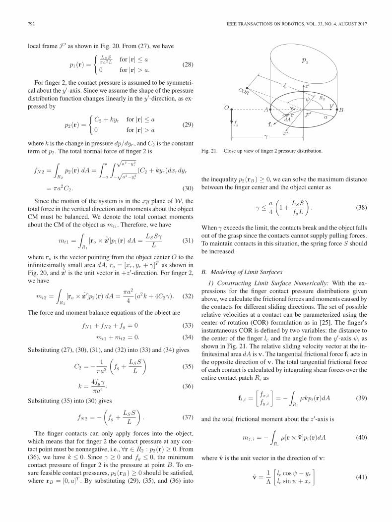
Fig. 21. Close up view of finger 2 pressure distribution.
the inequality p2(rB ) ≥ 0, we can solve the maximum distancebetween the finger center and the object center as
γ ≤ a
4
(1 +
LSS
fgL
). (38)
When γ exceeds the limit, the contacts break and the object fallsout of the grasp since the contacts cannot supply pulling forces.To maintain contacts in this situation, the spring force S shouldbe increased.
B. Modeling of Limit Surfaces
1) Constructing Limit Surface Numerically: With the ex-pressions for the finger contact pressure distributions givenabove, we calculate the frictional forces and moments caused bythe contacts for different sliding directions. The set of possiblerelative velocities at a contact can be parameterized using thecenter of rotation (COR) formulation as in [25]. The finger’sinstantaneous COR is defined by two variables: the distance tothe center of the finger lc and the angle from the y′-axis ψ, asshown in Fig. 21. The relative sliding velocity vector at the in-finitesimal area dA is v. The tangential frictional force ft acts inthe opposite direction of v. The total tangential frictional forceof each contact is calculated by integrating shear forces over theentire contact patch Ri as
ft,i =[fx,ify ,i
]= −
∫Ri
μvpi(r)dA (39)
and the total frictional moment about the z′-axis is
mz,i = −∫Ri
μ[r × v]pi(r)dA (40)
where v is the unit vector in the direction of v:
v =1Λ
[lc cosψ − yrlc sinψ + xr
](41)
SHI et al.: DYNAMIC IN-HAND SLIDING MANIPULATION 793
Fig. 22. Numerically integrated and approximated limit surfaces of finger 2.The axes of the friction force space are aligned with the local frame F′ andnormalized. Blue dots are the numerical integration results, green ellipsoidsshow the approximated limit surfaces.
Fig. 23. Numerically integrated and approximated limit surfaces when theCOR is moving along the y ′-axis, shown in the fxmz -plane. Blue dots arenumerical integration results, green ellipsoids show the approximated limitsurfaces.
where Λ =√l2c − 2yr lc cosψ + 2xlc sinψ + x2
r + y2r . Substi-
tuting (41) into (39) and (40), we have
ft,i =∫ a
−a
∫ √a2 −y 2
r
−√a2 −y 2
r
−μpi(r)Λ
[lc cosψ − yrlc sinψ + xr
]dxrdyr
(42)
mz,i =∫ a
−a
∫ √a2 −y 2
r
−√a2 −y 2
r
−μΦpi(r)Λ
dxrdyr (43)
where Φ = lcxr sinψ − lcyr cosψ + x2r + y2
r .The frictional forces and moments of finger 1 can be consid-
ered as a special case of finger 2, where γ = 0 and both p1 andp2 are constant. Therefore, we only analyze the limit surface forfinger 2.
Equations (42) and (43) do not have closed-form solutionssince they are elliptic integrals. Equations (35) and (36) can benumerically integrated to construct the limit surfaces. Figs. 22and 23 show the results of numerical integration of limit
surfaces of finger 2 with four different values of γ. Each bluedot represents an integration result of a COR position on thex′y′-plane (a pair value of lc and ψ). Substituting LS = 0.05m, L = 0.17 m, fg = − 0.5 N, S = − 7 N, a = 0.0254 m into(38), we find the maximum γ is γmax ≈ 1.279 a.
2) Approximation of the Limit Surfaces: Since the shape ofLS1 is a special case of LS2 when γ = 0, in this section wefocus on the derivation of the expression for the approximatedLS2 . The idea is to fit an ellipsoid to the numerical integralsin the local frame F′ that deforms as γ increases. This LSapproximation is then expressed in the local frame F+ , whichis used in the dynamics derived in Section V.
Observation 1: From Figs. 22 and 23, we observe that as thedistance γ from the object center to the finger center increases,the mz components of points on the limit surface increase ordecrease by a factor linear in both γ and fx .
From (37), the total normal force is not affected by γ, whichmeans that the maximum linear frictional force μfN2 will be thesame as long as γ ≤ γmax, and the projection of the limit surfacesto the fxfy -plane will be the same circle centered at the originwith radius μfN2 . Equation (36) shows that the contact pressuredistribution is determined by γ, which also affects the maximumfrictional moment mz,2 at each COR. Therefore as γ changes,the shape of the limit surfaces changes in the mz -direction.
Based on observation 1, we use deformed ellipsoidsto approximate the limit surfaces. We denote fF
′e =
[fx,e , fy ,e ,mz,e ]T as an arbitrary vector on an ellipsoid cen-tered at the origin of the local finger frame F′, and fF
′=
[fx, fy ,mz ]T as an arbitrary vector on the corresponding ap-proximated limit surface. The ellipsoid is represented by
(fF′
e )T AefF′
e = 1 (44)
where the matrix Ae ∈ R3×3 is a symmetric positive-definitematrix that determines the shape of the ellipsoid. In the gen-eral ellipsoid definition, Ae = diag(s−2
1 , s−22 , s−2
3 ) where s1 ,s2 , and s3 represent the lengths of the semiprincipal axes. Weagain assume isotropic dry friction so the maximum tangentialforce the contact can resist is s1 = s2 = μ|fNi
|. The maximummoment along the normal direction is s3 = caμ|fNi
|, where ais the radius of the contact patch and c is a constant from numer-ical integration. Here, we take c = 0.63 based on the findings in[25].
Since the limit surface is approximated by the ellipsoid de-formed linearly in the mz -direction proportional to fx , we have
mz = mz,e + κ(γ)fx,e (45)
where κ(γ) is a variable that determines the linear mapping.To deriveκ(γ), we choose a critical point fF
′∗ = [f ∗x , f
∗y ,m
∗z ]T
in the frame F′. Let f ∗x = μfN2 , f∗y = 0 so the projection of fF
′∗
in the fxfy -plane is at the edge of the limit circle. At this point,from the ellipsoid definition, we have m∗
z ,e = 0. From (45), wefind
κ(γ) = m∗z /f
∗x,e . (46)
794 IEEE TRANSACTIONS ON ROBOTICS, VOL. 33, NO. 4, AUGUST 2017
We calculate m∗z from (36) and (43) by substituting ψ = 0 and
lc = −∞
m∗z = −μ
∫ a
−a
∫ √a2 −y 2
r
−√a2 −y 2
r
yr (C2 + kyr )dxrdyr
= −μπa4k
4= −μfgγ. (47)
Since the ellipsoid is only deformed in the mz -direction, wehave f ∗x,e = f ∗x = μfN2 . Substituting this expression and (47)into (46), we have
κ(γ) =m∗z
f ∗x= −fgγ
fN2
. (48)
The transformation from the ellipsoid to the limit surface isgiven by (
fF′)T
=(fF
′e
)TD (49)
where D is an affine transformation matrix that deforms theellipsoid as
D =
⎡⎣1 0 κ
0 1 00 0 1
⎤⎦ .
From (44) and (49), we have (fF′)T D−1AeD−T fF
′= 1. The
expression for all the points on the limit surface can be writtenas (
fF′)T
Am fF′= 1 (50)
where
Am = D−1AeD−T =
⎡⎣ (κ2/s2
3 + s−21 ) 0 −κ/s2
30 s−2
2 0−κ/s2
3 0 s−23
⎤⎦ .
To describe the frictional limit surface in the frame F+ , wehave
fT =(fF
′)T
RF′F+(51)
where RF′F+is a transformation matrix that transfers the ref-
erence frame of linear force vectors from F′ to F+ and
RF′F+=
⎡⎣ sinφ − cosφ 0
cosφ sinφ 00 0 1
⎤⎦
where φ = tan−1( yr f 2xr f 2
), as shown in Fig. 6. From (50) and (51),
we write the equation of the limit surface in frame F+ as
fT Af = 1 (52)
where A = (RF′F+)−1Am (RF′F+
)−T .Comparisons showing the good agreement between the ap-
proximated frictional limit surface and the numerically inte-grated points are shown in Figs. 22 and 23.
REFERENCES
[1] D. E. Whitney, “Quasi-static assembly of compliantly supported rigidparts,” J. Dyn. Syst., Meas. Control, vol. 104, no. 1, pp. 65–77, 1982.
[2] S. Huang and J. M. Schimmels, “Admittance selection for force-guidedassembly of polygonal parts despite friction,” IEEE Trans. Robot., vol. 20,no. 5, pp. 817–829, Oct. 2004.
[3] N. Chavan-Dafle et al., “Extrinsic dexterity: In-hand manipulation withexternal forces,” in Proc. IEEE Int. Conf. Robot. Autom., May 2014,pp. 1578–1585.
[4] J. Shi, J. Woodruff, and K. Lynch, “Dynamic in-hand sliding manipula-tion,” in Proc. 2015 IEEE/RSJ Int. Conf. Intell. Robots Syst., Sep. 2015,pp. 870–877.
[5] Z. Li, P. Hsu, and S. Sastry, “Grasping and coordinated manipulation by amultifingered robot hand,” The Int. J. Robot. Res., vol. 8, no. 4, pp. 33–50,1989.
[6] T. Yoshikawa and K. Nagai, “Manipulating and grasping forces in manip-ulation by multifingered robot hands,” IEEE Trans. Robot. Autom., vol. 7,no. 1, pp. 67–77, Feb. 1991.
[7] N. Rojas and A. Dollar, “Characterization of the precision manipulationcapabilities of robot hands via the continuous group of displacements,” inProc. IEEE/RSJ Int. Conf. Intell. Robots Syst. Conf., Sep. 2014, pp. 1601–1608.
[8] D. Brock, “Enhancing the dexterity of a robot hand using controlled slip,”in Proc. IEEE Conf. Robot. Autom., Apr. 1988, vol. 1, pp. 249–251.
[9] A. Cole, P. Hsu, and S. Sastry, “Dynamic control of sliding by robot handsfor regrasping,” IEEE Trans. Robot. Autom., vol. 8, no. 1, pp. 42–52, Feb.1992.
[10] J. Trinkle and J. Hunter, “A framework for planning dexterous manipula-tion,” in Proc. IEEE Int. Conf. Robot. Autom., Apr. 1991, vol. 2, pp. 1245–1251.
[11] M. Yashima, Y. Shiina, and H. Yamaguchi, “Randomized manipulationplanning for a multi-fingered hand by switching contact modes,” in Proc.IEEE Int. Conf. Robot. Autom., vol. 2, Sep. 2003, pp. 2689–2694.
[12] R. Fearing, “Simplified grasping and manipulation with dextrous robothands,” IEEE J. Robot. Autom., vol. 2, no. 4, pp. 188–195, Dec. 1986.
[13] M. Cherif and K. K. Gupta, “Global planning for dexterous reorientationof rigid objects: Finger tracking with rolling and sliding,” The Int. J. Robot.Res., vol. 20, no. 1, pp. 57–84, 2001.
[14] N. Furukawa, A. Namiki, S. Taku, and M. Ishikawa, “Dynamic regraspingusing a high-speed multifingered hand and a high-speed vision system,”in Proc. IEEE Int. Conf. Robot, May 2006, pp. 181–187.
[15] N. Chavan-Dafle and A. Rodriguez, “Prehensile pushing: In-hand manip-ulation with push-primitives,” in Proc. 2015 IEEE/RSJ Int. Conf. Intell.Robots Syst., Sep. 2015, pp. 6215–6222.
[16] F. E. Vina, B. Y. Karayiannidis, K. Pauwels, C. Smith, and D. Kragic,“In-hand manipulation using gravity and controlled slip,” in Proc. 2015IEEE/RSJ Int. Conf. Intell. Robots Syst., Sep. 2015, pp. 5636–5641.
[17] F. E. Vina, B. Y. Karayiannidis, C. Smith, and D. Kragic, “Adaptivecontrol for pivoting with visual and tactile feedback,” in Proc. 2016 IEEEInt. Conf. Robot. Autom., May 2016, pp. 399–406.
[18] V. Kumar, E. Todorov, and S. Levine, “Optimal control with learned localmodels: Application to dexterous manipulation,” in Proc. 2016 IEEE Int.Conf. Robot. Autom., May 2016, pp. 378–383.
[19] A. Sintov and A. Shapiro, “Swing-up regrasping algorithm using en-ergy control,” in Proc. 2016 IEEE Int. Conf. Robot. Autom., May 2016,pp. 4888–4893.
[20] Y. Hou, Z. Jia, A. M. Johnson, and M. T. Mason, “Robust planar dy-namic pivoting by regulating inertial and gripping forces,” in WorkshopAlgorithmic Found. Robot., 2016.
[21] H. Arisumi, K. Yokoi, and K. Komoriya, “Casting manipulation—Midaircontrol of a gripper by impulsive force,” IEEE Trans. Robot., vol. 24,no. 2, pp. 402–415, Apr. 2008.
[22] S. Goyal, “Planar sliding of a rigid body with dry friction: Limit surfacesand dynamics of motion,” Ph.D. dissertation, Cornell Univ., Ithaca, NY,USA, 1989.
[23] S. Goyal, A. Ruina, and J. Papadopoulos, “Planar sliding with dryfriction—Part 1. Limit surface and moment function,” Wear, vol. 143,no. 2, pp. 307–330, 1991.
[24] S. Goyal, A. Ruina, and J. Papadopoulos, “Planar sliding with dry friction—Part 2. Dynamics of motion,” Wear, vol. 143, no. 2, pp. 331–352, 1991.
[25] N. Xydas and I. Kao, “Modeling of contact mechanics and friction limitsurfaces for soft fingers in robotics, with experimental results,” The Int. J.Robot. Res., vol. 18, no. 9, pp. 941–950, 1999.
[26] J. Zhou, R. Paolini, J. A. Bagnell, and M. T. Mason, “A convex polynomialforce-motion model for planar sliding: Identification and application,” inProc. IEEE Int. Conf. Robot. Autom., May 2016, pp. 372–377.
SHI et al.: DYNAMIC IN-HAND SLIDING MANIPULATION 795
Jian Shi received the B.S. degree in mechanical en-gineering and automation from Beihang University,Beijing, China, in 2011. He is currently working to-ward the Ph.D. degree in mechanical engineering atNorthwestern University, Evanston, IL, USA.
His research interests include motion planning andcontrol of dynamic robot manipulation.
J. Zachary Woodruff (S’15) received the B.S. de-gree in mechanical engineering from University ofNotre Dame, Notre Dame, IN, USA, in 2013, and theM.S. degree in mechanical engineering from North-western University, Evanston, IL, USA, in 2016. Heis a mechanical engineering Ph.D. candidate at North-western University in the Neuroscience and RoboticsLab (nxr.northwestern.edu).
His research interests include motion planningand control for hybrid dynamical systems with un-certainty.
Mr. Woodruff received the National Science Foundation Graduate ResearchFellowship in 2015.
Paul B. Umbanhowar received the B.A. degreein physics from Carleton College, Northfield, MN,USA, in 1987, and the Ph.D. degree in physics fromThe University of Texas at Austin, Austin, TX, USA,in 1996.
He is a Research Associate Professor in the De-partment of Mechanical Engineering, NorthwesternUniversity, Evanston, IL, USA, and an affiliate mem-ber of the Neuroscience and Robotics Laboratory.His research interests include locomotion on yield-ing substrates, frictional and vibratory manipulation,
and flow, segregation, and mixing of granular materials.
Kevin M. Lynch (S’90–M’96–SM’05–F’10) re-ceived the B.S.E. degree in electrical engineeringfrom Princeton University, Princeton, NJ, USA, in1989, and the Ph.D. degree in robotics from CarnegieMellon University, Pittsburgh, PA, USA, in 1996.
He is a Professor and the Chair of the MechanicalEngineering Department, Northwestern University,Evanston, IL, USA. He is a member of the Neuro-science and Robotics Laboratory and the Northwest-ern Institute on Complex Systems. His research inter-ests include dynamics, motion planning, and control
for robot manipulation and locomotion; self-organizing multiagent systems; andfunctional electrical stimulation for restoration of human function. He is a coau-thor of the textbooks Principles of Robot Motion (MIT Press, 2005), EmbeddedComputing and Mechatronics (Elsevier, 2015), and Modern Robotics: Mechan-ics, Planning, and Control (Cambridge University Press, 2017).