A comparative study of the UPFC system by simulation with PI-D and (NEWELM and NIMC) controllers based on the adaptive control for

the compensation of power

BOUANANE ABDELKRIM1, YAHIAOUI MERZOUG1, BENYAHIA KHALED1, CHAKER ABDELKADER2

1Department of Electrical Engineering,L.G.E Laboratory Dr. Mouly Taher University of Saida, Algeria

BP.138 el-Nasr Saida, ALGERIA E-mail: bouananeabd@ yahoo.fr, myahiaoui2001@yahoo.fr, kh.benyahia@yahoo.fr

2Department of Electrical Engineering, LGEER Laboratory ENPO oran ALGERIA

Abstract: -Flexible Alternating Current Transmission System devices (FACTS) are power electronic components. Their fast response offers potential benefits for power system stability enhancement and allows utilities to operate their transmission systems even closer to their physical limitations, more efficiently, with improved reliability, greater stability and security than traditional mechanical switching technology. The unified Power Flow Controller (UPFC) is the most comprehensive multivariable device among the FACTS controllers. According to high importance of power flow control in transmission lines, new controllers are designed based on the Elman Recurrent Neural Network (NEWELM) and Neural Inverse Model Control (NIMC) with adaptive control. The Main purpose of this paper is to design a controller which enables a power system to track reference signals precisely and to be robust in the presence of uncertainty of system parameters and disturbances. The performances of the proposed controllers (NEWELM and NIMC) are based neural adaptive control and simulated on a two bus test system and compared with a conventional PI controller with decoupling (PI-D). The studies are performed based on well known software package MATLAB/Simulink tool box.

Key-Words: - FACTS - UPFC - PI-D – NEWELM- NIMC- Neural Adaptive Control- Synthesis- Stability- Robustness.

Received: July 14, 2019. Revised: December 22, 2019. Accepted: January 14, 2020. Published: February 3, 2020.

1 Introduction The industrialization and the growth of the population

are the first factors for which the consumption of electrical energy increases regularly. In addition we live today in the era of electronics and informatics and any expenses are very sensitive to disturbances that occur on their supplies: a loss of power can cause the interruption of the different processes of the production; and in front of consumers who are becoming more demanding in wanting more energy and best quality, enterprises of production of electrical energy must therefore ensure the regular supply of this request, and without interruption, through a mesh network and interconnected in order to prove a reliability in their service; and increase the number of power plants, lines, transformers etc., which implies an increase of the cost and the degradation of the natural environment[14].The networks increased continuously And they becomes complex and more difficult to control. This system must drive in large quantities of energy in the absence of control devices and sophisticated adequate, a lot of problems can occur on this network such as: the transit of the reactive power in

excess in the lines, the hollow of voltage between different parts of the network…etc. and this fact the potential of the interconnection of the network will not operate properly. Up to the end of the eighties, the electrical networks were controlled by electromechanical devices having a response time of the more or less long, coils of inductance and Capacitors switched by circuit breakers for the maintenance of the voltage and the management of the reagent[4]. However, problems of wear as well as their slow action does not allow to operate these devices more than a few times a day, they are therefore difficult to use for a continuous control of the flow of power. Another technique of adjustment and control of reactive powers, tensions and transits of power using the power electronics has made its evidence.

The solution of these problems happening by improving the control of electrical systems already in place. It is necessary to equip these systems of a certain degree of flexibility allowing them to better adapt to the new requirements. The rapid development of the electronic power has had a considerable effect in the improvement of the conditions for the functioning of the

WSEAS TRANSACTIONS on ELECTRONICS DOI: 10.37394/232017.2020.11.4

Bouanane Abdelkrim, Yahiaoui Merzoug, Benyahia Khaled, Chaker Abdelkader

E-ISSN: 2415-1513 22 Volume 11, 2020

Vb V1

Ish T2

T1 Inverter (1) Inverter

( )

Vsh C

Vse

The The references Control

electrical networks in the performance of the control of their settings by the introduction of control devices on the basis of components of Electronic Power very advanced (GTO, IGBT) known under the acronym facts: "flexible alternating current transmission systems"[2,6,9,10].

The contribution of this technology "FACTS" (Narain and al ,1999)for the companies of the electricity is to open new prospects for controlling the flow of power in networks and to increase the capacity used existing lines similar to extensions in the latter. The UPFC consists of two voltage-source inverters with fully switchable elements (GTO, IGBT) that are connected through a common continuous link (DC-link). One, Mounted in shunt, called STATCOM (Static compensator), injects an almost sinusoidal current of adjustable magnitude. The second, mounted in series, called SSSC (Static Series synchronous compensator) [4, 7, 16, 21], injects in series an almost alternative voltage with an adjustable amplitude and phase angle in the transport line. Each inverter can swap the necessary reactive power locally, and produce the active power as a result of the serial injection of a voltage. The basic function of the shunt inverter (Inverter 1) is to supply or absorb the active power requested by the serial inverter (Inverter 2) through the common DC connection. It can also produce or absorb reactive power as required and provide voltage support at the network connection point.

Fig.1. Basic circuit configuration of a UPFC.

2. Modeling of A UPFC System

The equivalent crcuit of a UPFC system is shown in Fig. 2 where the series and shunt inverters are represented by voltage sources vc

and vp

respectively. The transmission

line is modeled [1, 3, 19, 28] as a series combination of resistance r and inductance L. The parameters rp and Lp

represent the shunt transformer resistance and leakage inductance respectively. The non linearity’s caused by the switching of the semiconductor devices, transformer saturation and controller time delays are neglected in the equivalent circuit and it is assumed that the transmission system is symmetrical. The simplified circuit of the UPFC control and compensation system is shown in Figure 2.

Fig.2. Equivalent circuit of UPFC system.

The modeling of this circuit is based on hypotheses simplifying. The dynamic equations of the UPFC are divided into three systems of equations. By performing d-q transformation, the current through the transmission line can be described by the following equations.

ωi ‐ i

v ‐v ‐v

‐ωi ‐ i v ‐v ‐v (1)

Similarly, the shunt inverter can be described by:

ωi

i v ‐v ‐v

‐ωi i v ‐v ‐v

(2)

By the use of power balance if one neglects the losses of the inverter it is possible to express the continuous voltage by:

V i V i ‐V i ‐V i (3)

The DC-link capacitor C must be selected to be large enough to minimize voltage transients

3. Controller Design

The control system of the UPFC consists of the shunt inverter with the control circuit [9, 11, 20], as well as the series inverter. First, we justify the possibility of separation of the two control circuits and similarly we are interested in the adjustment of the inverter for the additional voltage and more particularly to the setting of the active and reactive power transmitted.Then we will develop the different settings considered in this study and we will show the transient behavior of the control circuits using a simulation of the regulators considered in the adjustment of the closed loop UPFC system in order to improve the performances in the case of active or reactive power change. , (change one of the three parameters of the line).

3.1 PI decoupling control (PI-D):

The objective of using the is to provide independent control of active P and reactive Q power flow in the system for fixed values of Vs and Vr .This can be

WSEAS TRANSACTIONS on ELECTRONICS DOI: 10.37394/232017.2020.11.4

Bouanane Abdelkrim, Yahiaoui Merzoug, Benyahia Khaled, Chaker Abdelkader

E-ISSN: 2415-1513 23 Volume 11, 2020

achieved by properly controlling the series injected voltage of the UPFC. The voltage, current and power flow are related through the following equations. The principle of this control strategy is to convert the measured three phase currents and voltages into d-q values and then to calculate the current references and measured voltages as follow:

(4)

(5)

With and

∗ ∗ ∗

∆ (6)

∗ ∗ ∗

∆ (7)

With: ∆ (8)

According to the system of equations (1) or (2), one can have the system contains a coupling between the reactive and active current Id Iq .The interaction between current caused by the coupling term (ω) Fig. 3.

Fig.3. Control design with PI corrector.

To be able to lead to a reliable command of the system, it is indispensable to proceed to a decoupling of the two components. The decoupling of two loops is obtained by subtracting the term ( ) through a reaction against .It is then conducted to a rule which provides a command with decoupling (PI-D) of the currents Id and Iq with a model which can be rewritten in the following form:

1

1

(9)

The design of the control system must begin with the selection of variables to adjust and then that of the control variables and their association with variables set. There is various adjustment techniques well suited to the PI controller.The structure of the PI controller is represented by the first block diagram of Figure 4.

Fig. 4. Adjustment structure of the PI type.

In control, we obtain the following controller, depending on the damping coefficient and the frequency N :

2

2

Ni

Np

k

ak

(10)

There are two well-known empirical approaches proposed by Ziegler and Tit for determining the optimal parameters of the PI controller Table 1.

Table 1. OPTIMAL PARAMETERS OF THE PI CONTROLLER.

Type of regulator Kp Ti Kd

PI 0.45Kcr 0.83 Pcr 0

The method Ziegler-Nichols [29] used in the present article is based on a trial conducted in closed loop with a simple analogy proportional controller. The gain Kp of the regulator is gradually increased until the stability limit, which is characterized by a steady oscillation. Based on the results obtained, the parameters of the PI controller given by TABLE 2:

Table 2.PARAMETERS PI CONTROLLER IN OUR SYSTEM

Parameters Ki Kp ξ

Valeas 20.000 314.156 0.45 0.200

a. PERFORMANCE EVALUATION:

Simulation are performed a Pentium PC under MATLAB/Simulink software program. The transmission line and the UPFC (two inverters) system are implemented with simulink blocks.For each of the control systems, a simulation model is created which includes the required PWM.The parameters of the simulation model are selected to be equal to the parameters of a laboratory UPFC model [3] which are listed in TABLE 3.

Table 3. The parameters of the laboratory UPFC model

Vt = 220 V Vs = 220 V V*dc = 280 V C = 2 mF

Rp = 0.4 Ω Lp = 10 H R = 0.8 Ω

L = 10 H

Lrs /

1

y

refy

d

s

kk i

p

WSEAS TRANSACTIONS on ELECTRONICS DOI: 10.37394/232017.2020.11.4

Bouanane Abdelkrim, Yahiaoui Merzoug, Benyahia Khaled, Chaker Abdelkader

E-ISSN: 2415-1513 24 Volume 11, 2020

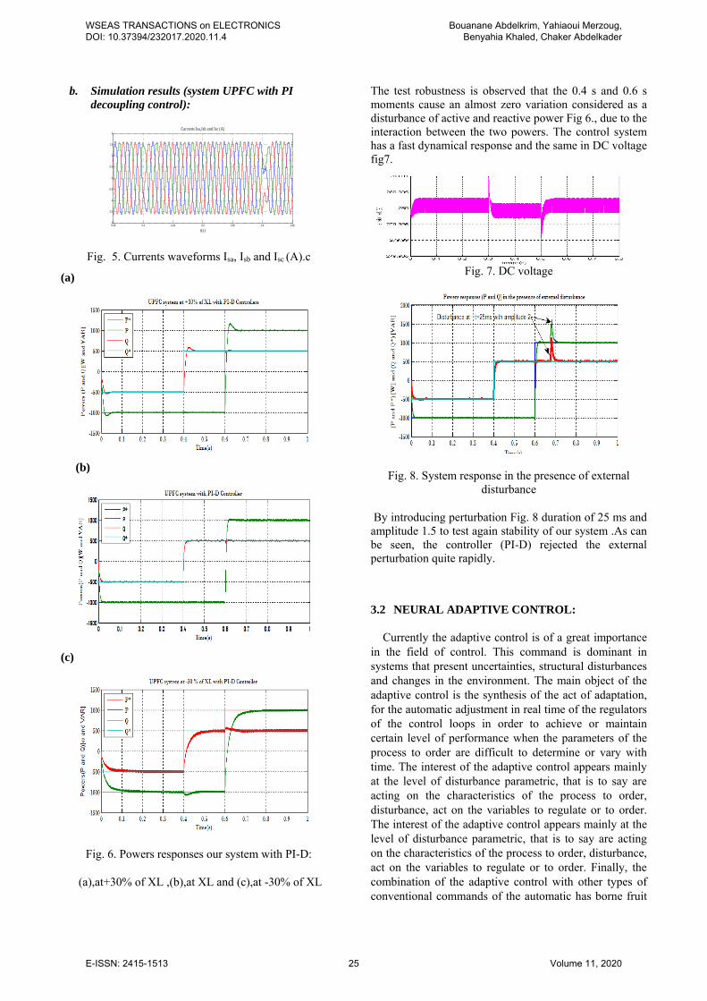
b. Simulation results (system UPFC with PI decoupling control):

Fig. 5. Currents waveforms Isa, Isb and Isc (A).c

(a)

(b)

(c)

Fig. 6. Powers responses our system with PI-D:

(a),at+30% of XL ,(b),at XL and (c),at -30% of XL

The test robustness is observed that the 0.4 s and 0.6 s moments cause an almost zero variation considered as a disturbance of active and reactive power Fig 6., due to the interaction between the two powers. The control system has a fast dynamical response and the same in DC voltage fig7.

Fig. 7. DC voltage

Fig. 8. System response in the presence of external disturbance

By introducing perturbation Fig. 8 duration of 25 ms and amplitude 1.5 to test again stability of our system .As can be seen, the controller (PI-D) rejected the external perturbation quite rapidly.

3.2 NEURAL ADAPTIVE CONTROL:

Currently the adaptive control is of a great importance in the field of control. This command is dominant in systems that present uncertainties, structural disturbances and changes in the environment. The main object of the adaptive control is the synthesis of the act of adaptation, for the automatic adjustment in real time of the regulators of the control loops in order to achieve or maintain certain level of performance when the parameters of the process to order are difficult to determine or vary with time. The interest of the adaptive control appears mainly at the level of disturbance parametric, that is to say are acting on the characteristics of the process to order, disturbance, act on the variables to regulate or to order. The interest of the adaptive control appears mainly at the level of disturbance parametric, that is to say are acting on the characteristics of the process to order, disturbance, act on the variables to regulate or to order. Finally, the combination of the adaptive control with other types of conventional commands of the automatic has borne fruit

0.35 0.4 0.45 0.5 0.55 0.6 0.65-2

-1.5

-1

-0.5

0

0.5

1

1.5

2Currents Isa,Isb and Isc (A)

t(s)

WSEAS TRANSACTIONS on ELECTRONICS DOI: 10.37394/232017.2020.11.4

Bouanane Abdelkrim, Yahiaoui Merzoug, Benyahia Khaled, Chaker Abdelkader

E-ISSN: 2415-1513 25 Volume 11, 2020

and has been the source of many jobs. The adaptive laws implanted in the ideal case could lead to instability in the case of external disturbances bounded.

In this article we present the Adjustment method proposed for the UPFC, favoring the classical approach based on neurons networks. Neural Network is trained by adaptive learning [3, 22, 27], the network ‘learns’ how to do tasks, perform functions based on the data given for training. The knowledge learned during training is stored in the synaptic weights. The standard Neural Network structures (feed forward and recurrent) are both used to model the UPFC system. The main task of this paper is to design a neural network controller which keeps the UPFC system stabilized. Elman's network [26] said hidden layer network is a recurrent network, thus better suited for modeling dynamic systems. His choice in the neural control by state feedback, is justified by its role, this network can be interpreted as a state space model nonlinear. Learning by back propagation algorithm standard is the law used for identification of the UPFC.

Fig. 9. Structure of the Elman network

A. Neural Adaptive Control by State Space UPFC System with ERNN (NACSSS-ERNN):

The integration of these two approaches (neural adaptive control ) in a single hybrid structure, that each benefits from the other, but to change the dynamic behavior of the UPFC system was added against a reaction calculated from the state vector (state space) Fig. 7.

Fig. 10. Diagram of a UPFC control by state feedback The state feedback control is to consider the process

model in the form of an equation of state: ∗ (11) And observation equation: (12) Where u (t) is the control vector, x (t) the state

vector, and y (t) the output vector of dimension for a discrete system to the sampling process parameters Te at times of Te sample k are formalized as follows:

X 1 (13) (14) The system is of order 1, so it requires a single state

variable x. this state variable represents the output of an integrator as shown in Fig.

x(t) = y(t) x* (t) = y*(t)

Fig. 11. Block diagram of the state representation of the UPF

The transfer function G s Y s U s⁄ of our

process UPFC can be written as:

G s ⁄

(15)

We deduce the equations of state representation of the UPFC:

∗

(16)

With: U t e t kx t Let:X t 1 x t e t (17) (18) The dynamics of the process corrected by state space

is presented based on the characteristic equation of the matrix [Ad - Bd K], where K is the matrix state space controlled process. Our system is described in matrix form in the state space:

Where:∗

(19)

,

10

01 , 1 0

0 1, 0 0

0 0

, ,

a. UPFC SYSTEM IDENTIFICATION USING ERNN( NEWELM) :

The identification makes it possible to obtain a mathematical model that represents as faithfully as possible the dynamic behavior of the process [5, 17].

A process identified will then be characterized by the structure of the model, of its order and by the values of the Settings .It is therefore, a corollary of the process simulation for which one uses a model and a set of coefficients in order to predict the response of the system.

The figure shows the network Elman consisting of three layers: a layer of entry, hidden layer and a layer of output. The layers of entry and exit interfere with the outside environment, which is not the case for the intermediate layer called hidden layer. In this diagram, the entry of the network is the command U(t) and its

Input layer Hidden layer Output layer

y*=x* U Y=x +

L

r

UPFC System

K

E (t) U (t) Y (t)

X (t)

+

WSEAS TRANSACTIONS on ELECTRONICS DOI: 10.37394/232017.2020.11.4

Bouanane Abdelkrim, Yahiaoui Merzoug, Benyahia Khaled, Chaker Abdelkader

E-ISSN: 2415-1513 26 Volume 11, 2020

output is Y (t) .The vector of state X(t) from the hidden layer is injected into the input layer.

Fig. 12. Structure of the NEWELM The state vector X (t) from the hidden layer is

injected into the input layer. We deduce the following equations: X t W X t 1 W U t 1 (20)

Y t W X t (21)

Where, Wh ; Wr et Wo are the weight matrices. Equations are standard descriptions of the state space of dynamical systems. The order of the system depends on the number of states equals the number of hidden layers. When an input-output data is presented to the network at iteration k squared error at the output of the network is defined as:

(22)

For the whole training data u (t), yd (t) de t = 1, 2… N, the summed squared errors is:

∑ (23)

The weights are modified at each time step for W0 :

. (24)

For Wh et Wr,

. .

. 0. (25)

.ķ.

. . (26)

The latter we obtain:

1 (27)

Equation shows that there is a dynamic trace of the gradient. This is similar to back propagation through time. Because the general expression for weight modification in the gradient descent method is:

(28)

The dynamic back propagation algorithm used to identify a state space model of the UPFC for NEWELM (Elman network) can be summarized as follows:

(29)

. (30)

. (31)

If the dependence of X (t-1) on Wi is ignored, the above

algorithm degretes is the standard back propagation

algorithm:

1 (32)

Fig. 13. UPFC system presentation with state space and (ERNN-NEWELM).

Note that the performance of the identification is

better when the input signal is sufficiently high in frequency to excite the different modes of process. The three weights Wo ,Wr and Wh which are respectively the

Network with ERNN-NEWELM

Input layer

Hidden layer

y(t)W0

x(t)

Wr

Wh

U(t)

Output layer

UPFC with SSNN

e (t) = i*sd

u (t) = vcd

v (t) = id

K

WSEAS TRANSACTIONS on ELECTRONICS DOI: 10.37394/232017.2020.11.4

Bouanane Abdelkrim, Yahiaoui Merzoug, Benyahia Khaled, Chaker Abdelkader

E-ISSN: 2415-1513 27 Volume 11, 2020

matrices of the equation of state of the process system (UPFC) [C, A and B] became stable after a rough time t = 0.3s and several iterations fig. 9.NB . For the NEWELM is assumed through the vector is zero (D = 0).

In online learning Elman network, the task of identifying and correcting same synthesis are one after the other. Or correction of the numerical values of the parameters is done repeatedly so the estimation error Fig. 10 takes about almost a second (t = 1s) to converge to zero ie regulation in pursuit

a. Estimation of the parameters:

The input used of the Echelon type, is envisaged for identification systems [15]. It is obvious that the entry is better than on the other (rail, Sinusoid……) from the point of view of the identification. In order to allow an identification by entries to excite the maximum of the modes of the system without too disrupt its normal operation, if it wants to pull a lot of information, in particular the excite in the entire frequency band interesting, one uses in general a variation in the niche market of pseudorandom binary sequence (PRBS) Superim The design of a system of efficient regulation and robust requires knowing the dynamic model of the process, which describes the relationship between the variations of the command and the variations of the measure. The dynamic model can be determined by direct identification.

The classic method type "Response Level"

requires signals of excitation of large amplitudes; its accuracy is reduced, and does not allow the validation of the model.

The current methods, with algorithms for recursive identification on micro computers offer a better precision and operate in open or closed loop mode with excitation signals of very low amplitude (0.5 to 5 per cent of the op pseudo random binary sequence (PRBS), and rich in frequency.

The Pseudo Random Binary Sequence (PRBS) is a signal consisting of rectangular pulses modulated randomly in length, which approximate a white noise discreet, therefore rich in frequency and average value of zero, not amending the operating point of the process. Easy to generate; it is commonly used in the identification procedures. Posed on useful signal.

Therefore, in our project it was used for the identification of the parameters of the system a network neuron said network of Elman with three layers .As has already been seen. Note that the performances of the identification are best when the input signal is rich

enough in frequencies to excite the different modes of process.

To obtain its results, a pseudo random binary sequence ( PRBS) is used as the excitation signal and are of the estates of rectangular pulses modulated in width, which are approximate to a white noise discrete which have a rich content of frequencies.

For the simulation it was chosen: Network Elman (NEWELM) to three layers

[Entry, hidden and output] is respectively [vector command, the vector of state and output vector]

A rich signal of frequency pseudorandom binary sequence is of languor in 1023 and of amplitude 1V.

A PRBS signal fig 14. Is input to system to provide reasonable convergence of the neural network weights for the controller to start with.

Fig. 14. PRBS signal and changing weights

There is after the application of pseudorandom binary sequence (PRBS) signal that the pace of three weights wo, wr and wh who are respectively the matrices of the equation of state of the process (UPFC system).[C, A and B] are become stable after an approximate time t=0.3s and several iterations and [D] equal to zero for the NEWELM figure15.

Fig. 15. Estimation error

In online learning the network Elman fig.15, the tasks of identifying, synthesis and correction are one after the other, where the correction of the numerical values of the parameters is made of recurring ways so the error of the estimate is approximately almost a second (t=1s) to converge toward zero the flowing of results with Fig. 19.

WSEAS TRANSACTIONS on ELECTRONICS DOI: 10.37394/232017.2020.11.4

Bouanane Abdelkrim, Yahiaoui Merzoug, Benyahia Khaled, Chaker Abdelkader

E-ISSN: 2415-1513 28 Volume 11, 2020

B. Neural adaptive control by internal model of a

UPF system (NACIMS):

Several techniques can be envisaged in order to improve the performance. In this work, we use the command by internal model, which belongs to the family of commands in a closed loop (feedback). Its principle is call to a model of the system and has the property to operate in quasi open loop as long as the system and their models are identical, which reduces the risks of instability encountered in the technical standards of counter-reaction. This solution can be used on any architecture or technology of the chain because the only elements to be added are a couple and a demodulator to the issuance to retrieve information on the distortions introduced. In order to assess the performance of this technique, we have applied in simulation on our system UPFC.

a. Internal Model Control:

Figure 16 represents the basic scheme of IMC. For reasons of simplicity, it illustrates the general principle on a linear system in the field of Laplace knowing that this representation can be extended to the discrete domain.

Fig. 16. Basic scheme of IMC

In this figure, we find the main elements of a feedback loop:

The system H(s), output y(t), The model of the system, obtained by

prior identification of the system, The corrector R(s), The set point or the excitation e(t), A disturbance d(t).

The study of the structure makes it possible to establish the following operating equation, linking the output Y to the input E and the perturbation D:

.

..

.

.. (32)

The error of characterization (or modeling) the system that represents the difference between the system and its model is represented by the term:

(34)

The errors signal w (t) rebuilt the disturbance D (t) and the error of characterization following the command u (t):

. (36)

So we can say that the stability of the whole when R(s) and are stable. For an ideal model and a perfect pursuit of trajectory

, ∀ d (t)

An online estimate of unmeasured disturbances

(37)

b. Neural Inverse Model Control Design:

It is quite obvious that this excludes many cases, and thus the effective implementation of the IMC structure goes through techniques which are in two general principles: Minimize the sensitivity of the IMC structure for

maximum disturbance rejection Maximizing the complementary sensitivity for a

better pursuit

In the basic principle of the internal model control, the closer the model is to reality the more the structure approaches an open-loop structure. A closed loop type corrector can therefore compensate for this handicap while enlarging the class of systems for which the structure is applicable. On the other hand, the gap between the actual system and its behavioral model may be due to multiple reasons, so it is more reasonable to consider this signal as exogenous to the control. The structure of Figure 16 is modified as shown in Figure 17 [1].

Figure 17 Block diagram of IMC with input disturbance

The model M is determined by the Widrow-Hoff learning law [25] .The training of the network consists in modifying, with each step, the weights and bias in order to minimize the quadratic errors at output by using the law of Windrow-Hoff. With each step of training, the

e(t)

H (s)

H(s) R(s)

d

Filtering model

Controller C

Model

System P G(s)

Desired output

+ + + -

WSEAS TRANSACTIONS on ELECTRONICS DOI: 10.37394/232017.2020.11.4

Bouanane Abdelkrim, Yahiaoui Merzoug, Benyahia Khaled, Chaker Abdelkader

E-ISSN: 2415-1513 29 Volume 11, 2020

error at output is calculated as the difference between the required target t and the output y of the network. The quantity to be minimized, with each step of training k, is the variance of the error at the output of the network.

2 (38)

Te: The sampling time is equal to 1ms .This time will be maintained throughout this study.

The estimation of output and the error are calculated by:

1 1 ;

(39)

The learning of the network of neuron is to modify, at each sampling, the weight and bias (estimation of parameters) in order to minimize the quadratic criterion of the squares of the errors in the output.

The inverse model controller y (t) is given by the following equation:

1 (40)

Where:

1 2 (41)

So the weights and the bias fig. 18 are calculated as

follows: , and

The control law is described by: with

and

1 2 (42)

Fig. 18. Evolution of the weights and Estimation error (NACIM)

a. simulation with NACSS-NEWELM

Fig. 19. Powers (P and Q) of the control system with

( NACSS-NEWELM) at ± 30% of XL

Time (s)

Evolution of the Weights NACIMS

WSEAS TRANSACTIONS on ELECTRONICS DOI: 10.37394/232017.2020.11.4

Bouanane Abdelkrim, Yahiaoui Merzoug, Benyahia Khaled, Chaker Abdelkader

E-ISSN: 2415-1513 30 Volume 11, 2020

b. simulation with NACIMS

Fig. 20. Powers (P and Q) of the control system with

(NACIMS) at ± 30% of XL

4. Comparative simulation studies between NACSS-NEWELM and NACIMS:

Adaptive Neural Feedback Control (ANFC) is a hybrid control that has allowed them to control any variation in tracking, regulation or stability. The results of the simulation showed the strength of our neural adaptive controller (NAC).We can say that the decoupled PI regulator would be ideal for the UPFC system control if

the ± 30% variation of the reactance did not degrade its dynamic performance, as pointed out in this article. The process model is never perfect.The results of this analysis of the two controls by neural networks at ± 30% of XL fig.19 are summarized in the following points:

All control strategies indicate that the proposed regulators have better dynamic performance and are much more robust than the traditional PI controller. They seem to be very high performance dynamic regulators.

Thanks to the generalization capacity of network neurons, the use of a neural identification regulator allows an improvement in the dynamic performance of the regulator approached. It has even been demonstrated by simulation that a neural identification regulator can solve the problem of the incapacity of parametric variations regulator PI of the line.

5. Conclusions

In this article, our UPFC system based on three robust control methods has been proposed. As the controller (PI – D) and approach the control of neural adaptive applied on (NEWELM and NIMC). These control strategies introduce enough flexibility to set the desired level of stability and performance. Practical constraints were considered by introducing appropriate uncertainties. The methods above have been applied to a typical test of a single-phase power system bridge. Simulation results showed that designed regulators were able to ensure a robust stability and performance a wide range of uncertainty of parameters of transmission .but line orders two hybrid (NACSSS-ERNN and NACIMS) in case of modification of the parameters of the system and an excellent ability to improve the stability of the system under small disturbances.

References: [1] Alf Isaksson” Model based control design Supplied

as supplement to course book inAutomatic Control Basic” course (Reglerteknik AK) September, 1999.

[2] B.A. Renz, A. Keri, A.S. Mehraben, C. Schauder, E. Stacey, I. Kovalsky, L. Gyugyi, and A. Edris, 1999, “AEP Unified Power Flow Controller Performance”, IEEE Trans. on Power Delivery, 14(4), pp. 1374-1381.

[3] Bouanane A. ,Chaker A. and Amara M. “adaptive control with SSNN of UPFC system for compensation of active and reactive power”. Res J. Appl. Sci. Eng. Technol. Vol 6(4):739-747,2013.

[4] Ch. Praing, T. Tran-Quoc, R. Feuillet, J.C Sabonnadiere, J. Nicolas, Boi K. Nguyen “Impact of FACTS devices on voltage and transient stability of a power system including long transmission lines’’, IEEE Transactions on Power Engineering Society. Vol. 3 , pp. 1906 - 1911,2000.

WSEAS TRANSACTIONS on ELECTRONICS DOI: 10.37394/232017.2020.11.4

Bouanane Abdelkrim, Yahiaoui Merzoug, Benyahia Khaled, Chaker Abdelkader

E-ISSN: 2415-1513 31 Volume 11, 2020

[5] Delgado,A. and al (1995) “dynamic recurrent neural networks for system identification and control” IEE Proc.Control Theory Applications, Vol 142,n°4,pp.307-314.

[6] Gyungui. L, FIEE. (2008) ‘Unified Power Flow Control concept for Flexible AC Transmission System’ IEE proceedings- C, Vol.139, No.4

[7] H. Johal and D. Divan, “ Design considerations for series –connected distributed FACTS converters”, IEEE Transactions on industry applications, Vol.43,PP: 1609-1618, Nov/Dec. 2007.

[8] Henriques, J. and A. Dourado, 1999. A hybrid neural- decoupling pole placement controller and its application. Proceeding of 5th European Control Conference (ECC99). Karlsruhe, Germany.

[9] Hideaki Fujita, Yasuhiro Watanabe, Hirofumi Akagi, “Control and Analysis of a Unified Power Flow Controller”, IEEE TRANSACTIONS ON POWER ELECTRONICS, VOL. 14, NO. 6 November 1999, pp.1021-1027.

[10] J. Bian, D.G. Ramey, R.J. Nelson, and A. Edris, 1997, “A Study of Equipment Sizes and Constraints for a Unified Power Flow Controller”, IEEE Trans. on Power Delivery, 12(3), pp. 1385-1391.

[11] Kannan. S, Shesha Jayaram and M.M.A.Salama. (2007) ‘Real and Reactive Power Coordination for a Unified Power Flow Controller’ IEEE Transactions on Power Systems, 2007, vol.19.No.3, pp. 1454 – 1461.

[12] K.K. Sen, 1998, “SSSC – Static Synchronous Series Compensator: Theory, Modeling and Application”, IEEE Trans. on Power Delivery, 13(1), pp. 241-246.

[13] L. Gyugyi, C.D. Schauder, S.I. Williams, T.R. Reitman, D.R. Torgerson, and A. Edris, 1995, “The Unified Power Flow Controller: A new approach to power transmission control”, IEEE Trans. on Power Delivery, 10(2), pp. 1085-1097.

[14] L. Gyugyi, 1994, “Dynamic Compensation of AC Transmission Line by Solid State Synchronous Voltage Sources,” IEEE Transactions on Power Delivery, 9(22), pp. 904-911.

[15] M. I. Marei, "A unified control strategy based on phase angle estimation for matrix converter interface system," IEEE Systems Journal, vol. 6, no. 2, pp. 278-286, 2012.

[16] Narain, G.H. and G. Laszlo, 1999. Understanding FACTS: Concepts and Technology of Flexible AC Trnasmission Systems. Wiley-IEEE Press Marketing, pp: 297-352; 407-424.

[17] Narendra K.,Parthasarathy K.(1990) “identification and control of dynamical systems using neural networks” ,IEEE Trans. Neural Networks ,Vol 1 ,pp4-27 .

[18] Nguyen, D. and B. Widrow, 1990. Neural networks for self-learning control systems. IEEE Control Syst. Mag., 10(3): 18-23.

[19] P. Jagtap and N. Sharma, "Modelling and Application of Unified Power Flow Controller (UPFC)," Emerging Trends in Engineering &

Technology, International Conference (ICETET), Goa, India, 2010, pp. 350-355.

[20] Papic, I., P. Zunko, D. Povh and M. Weinhold, 1997.Basic control of unified power flow controller. IEEE T. Power Syst., 12(4): 1734-1739.

[21] R. Mohan Mathur and R. K. Varma. Thyristor-based FACTS Controllers for Electrical Transmission Systems, IEEE Series on Power Engineering, US, 2002.

[22] Reaz, M.B.I., Wei, L.S.: Adaptive linear neural network Ölter for fetal ECG extraction. In: The International Conference on Intelligent Sensing and Information Processing. (2004) pp.321-324.

[23] S Kannan Real & Reactive power coordination for UPFC, IEEE Transaction on power system vol19 n0 3 Aug 2004

[24] Sen, K.K. and A.J.F. Keri, 2003. Comparison of field results and digital simulation results of voltage- sourced converter-based facts controllers. IEEE.T. Power Deliver., 18: 300-306.

[25] Widrow, B., Lehr, M.A “ 30 years of adaptive neural networks: Perceptrons, madeline and backpropagation”. Proc. of IEEE 78 (1990) 1415ñ1442

[26] Xiang, L., C. Guanrong, C. Zengqian and Z. Yuan, 2002. Chaotifying linear Elman networks. IEEE T. Neural Networ., 13(5): 1193-1199.

[27] Xie, J.X., C.T. Cheng, K.W. Chau and Y.Z. Pei, 2006. A hybrid adaptive time-delay neural network model for multi-step-ahead prediction of sunspot activity. Int. J. Environ. Poll., 28: 364-381

[28] Zhengyu, H., N. Yinxin, C.M. Shen, F.F. Wu,C. Shousun and Z. Baolin, 2000. Application of unified power flow controller in interconnected power systems-modeling, interface, control strategy and case study. IEEE T. Power Syst., 15: 817-824.

[29] Ziegler, J.G. and N.B. Nichols, 1942. Optimum settings for automatic controllers. Trans. ASME, 64: 759-768.

WSEAS TRANSACTIONS on ELECTRONICS DOI: 10.37394/232017.2020.11.4

Bouanane Abdelkrim, Yahiaoui Merzoug, Benyahia Khaled, Chaker Abdelkader

E-ISSN: 2415-1513 32 Volume 11, 2020