A manufacturing network design model based on processor ...

A manufacturing network design model based on processor and worker capabilities

Marc Paquet,

Alain Martel

and

Benoit Montreuil

April 2005

Working Paper DT-2005-AM-1

(Revised March 2006)

Network Organization Technology Research Center (CENTOR),

Université Laval, Québec, G1K 7P4, Canada

© Centor, 2006

DT-2005-AM-1 1


Marc Paquet1, 2, Alain Martel1 and Benoit Montreuil1, 3, 4 1 CENTOR Research Center

Faculté des sciences de l’administration Université Laval Québec (Québec), CANADA, G1K 7P4

2 Department of Automated Manufacturing Engineering École de technologie supérieure 1100, Notre-Dame Ouest Montréal (Québec), CANADA, H3C 1K3 Corresponding Author: [email protected]

3 Canada Research Chair in Enterprise Engineering

4 NSERC/Bell/Cisco Business Design Research Chair Abstract

This paper presents an optimization methodology to design networks of manufacturing

facilities producing several products under deterministic demand. The bill of materials and

the operations for each product are taken into account through the use of a product-state

graph. Starting from the current state of the manufacturing network, the approach considers

a multi-period planning horizon. For each period it specifies the facilities to open within the

set of current and potential facilities, the mission for each of the centers in the selected

facilities, the equipment to be used for producing the goods, and the structure of the

network. Taking human resource competencies into account, the approach selects the type

of workers to use for executing the manufacturing tasks. The transfer of resources between

plants is also considered. A multi-period mixed integer linear programming model is

formulated, a solution method based on the addition of specialized cuts is proposed and

computational results are presented.

Keywords

Logistics, Supply Chain Design, Manufacturing Network Design, Location-Allocation,

Mixed Integer Programming (MIP)


DT-2005-AM-1 2

1. Problem Context

This paper presents an optimization methodology to design manufacturing networks under

deterministic demand. In a previous paper, a static network design model including

technology selection decisions was proposed (Paquet et al., 2004). The present work

extends our previous approach by considering the evolving needs of a network of multiple

production center plants over a multi-period planning horizon, and incorporating

manufacturing resources (processors and workers) assignment decisions based on their

respective capabilities. This kind of decision is critical in many industrial sectors such as

semi-conductors, optics-photonics, electronics and telecommunications. Product-state

graphs, similar to classical operation process charts, are used to describe the production

process of the manufactured products, as illustrated in Figure 1.

Figure 1: Manufacturing Product-State Graph

This graph can be derived from the bill-of-material (BOM) graph and the sequence of

operations required to manufacture each BOM-product, as illustrated in Figure 2. In this

figure, products 1, 2 and 3 are raw materials, product-states 43 (read Product 4, Process 3),

54, 63 and 73 are manufactured products, and product-states 85 and 95 are finished

products. These end-of-process products can be stored, they can be transferred between

production centers in a plant and between plants, and they can be shipped to customers. The


DT-2005-AM-1 3

other product-states in Figure 1 are intermediate parts which can be transferred between

centers, but cannot be stored or shipped between plants. These product-states correspond to

manufacturing processes required to build the part. All product-states require various

resources to be produced.

Figure 2: Product Graph & Production Processes

This work is related to several publications in the Supply Chain Design field. Early work

on facility location problems with capacity expansion and technology selection is well

documented in Verter and Dincer (1992), while Revelle and Laporte (1996) discuss many

possible extensions. The modeling advances include concepts like multiple production

echelons in the manufacturing network, plant loading, economies of scale and scope,

international issues, suppliers selection, outsourcing, etc. Cohen and Moon (1990), Cohen

and Moon (1991), Mazzola and Schantz (1997) and Verter and Dasci (2002) take into

account economies of scale and scope in their models. Benjaafar and Gupta (1998) and

Paquet et al. (2004) discuss technology choice and capacity planning decisions in a

manufacturing network. Benjaafar and Sheikhzadeh (2000) discuss the importance of

flexible technology at a manufacturing site. The selection of suppliers is also an important

issue as discussed in Vonderembse and Tracey (1999). Lakhal et al. (2001) propose a

model to determine the activities to outsource. Dogan and Goetschalckx (1999) introduce a

multi-season design model. The models proposed by Cohen et al. (1989), Arntzen et al.

(1995), Cordeau et al. (2002) and Martel (2005) include many of these critical supply chain

design aspects and they are among the most comprehensive models published to date. The

evolution of strategic logistic network design models is discussed in Geoffrion and Powers


DT-2005-AM-1 4

(1995). Shapiro (2001) also discusses several strategic and tactical supply chain planning

issues.

Important weaknesses of current manufacturing network design models are the lack of

consideration of manufacturing operations, of the organization of plants into production

centers, and of the impact worker competencies may have in some industrial sectors. Also

most models in the literature are static: they do not consider evolving production needs,

which can be crucial when product life-cycles are relatively short. This paper proposes a

design model addressing these issues. The structure of the network, the transfer of

resources (processors and workers) between plants, the customer service assignments and

the choice of raw material suppliers, over a multi-period planning horizon, are also taken

into account by the proposed model. Section 2 presents the model formulation details.

Section 3 discusses the solution method, section 4 presents the experimental evaluation of

the model and section 5 concludes the paper.

2. Model Formulation

The structure of the manufacturing network considered is illustrated in Figure 3, where

only a subset of the demand zones and outbound flows are illustrated. The model considers

a set of planning periods which could cover half a year to several years depending on the

industry context, and it takes into account the initial state of the network.

Some plants are in use at the beginning of the design process. These plants have resources

(processors and workers with different capabilities organized in production centers). Some

of these plants can be closed by the model and new plants can be opened on predetermined

sites. The configuration of production centers can be adjusted (processor types and required

workers). The demand nodes are predetermined and correspond to retailers, warehouses or

customer zones. These nodes require finished products and spare parts under a

deterministic demand scenario obtained from a set of forecasts based on product life cycle

curves. The network operates in a just-in-time or make-to-order manufacturing context and,

hence, there is no need to plan for significant inventory storage centers to support customer

demand in the network.


DT-2005-AM-1 5

Figure 3: Potential and Current Manufacturing Network for Finished Products P85 & P95

The raw materials come from potential supplier nodes. Limited amounts of each of the raw

materials are available from each of the suppliers. The model selects the best supply

sources. The manufacturing sites are characterized by a limited space for processors. These

processors have a limited capacity and their capabilities are linked to the product-state

graph of Figure 1. Specific worker types are required for each product-state on these

processors. Human resources are modeled separately of processor resources because they

use several processors in their work. The workers taken into consideration in the model are

specialists and they may be difficult to find on specific labor markets. They are therefore

strategic resources for the firm and their hiring and use must be planned carefully. All

workers are flexible within their capability limits. They are not allocated to a specific

processor. They can be assigned to any of the different product-states for which they have

the required competencies in a specific center.

Resource choices are possible for a given product-state, as illustrated in Figure 4.

Substitutions are possible between processors and also between workers. The resources

have capabilities, e.g. they can produce a limited set of product-states and they have

different processing times and costs. For human resources, highly qualified workers can


DT-2005-AM-1 6

perform lower level tasks (hierarchy of capabilities), but they cost more then less qualified

workers (Vercellis, 1991). The highly qualified workers may also be more difficult to find

on specific labor markets. In Figure 4, worker type capability hierarchies are illustrated. In

each of these hierarchies, higher number worker types are more qualified than lower

number worker types, i.e. in a given hierarchy, a worker type can perform the tasks of

preceding worker types. The resources (processors and workers) can be moved from a

manufacturing node to another and workers can be laid-off or hired at a specific plant.

Overtime can also be used to provide additional capacity during a planning period. It is

assumed that the capacity consumption of all resources is linear and that all available time

can be used.

Figure 4: Resource Capabilities

A production center is defined by a specific mission related to the product-states it can

produce and the potential resource types it has to produce these product-states. Four types

of center are distinguished (see Montreuil and Lefrançois (1996) and Montreuil et al.

(1998) for a discussion of center types and missions), as illustrated in Figure 5: product

centers (grouping of product-states by product, as shown in Figure 1), function centers

(grouping of product-states by process / shape, as shown in Figure 4), product group


DT-2005-AM-1 7

centers (grouping of two or more products) and process centers (grouping of two or more

consecutive processes required in more than one product). Each type of center has a unit

material handling cost, a total availability (e.g. a work shift) over the planning horizon and

a specific efficiency for its resources. This efficiency reflects the extent to which the

resources can be used in a particular type of production center. For example, for the

manufacturing of a specific product and all its parts, product centers are more efficient than

the corresponding set of function centers because they require less product handling

between processors.

Figure 5: Examples of Potential Production Center with Specific Missions

To formulate the model, the following sets are required:

P: Nodes of the product-state graph. B ⊂ P: Raw materials. M ⊂ P: Product-states of manufactured products. O ⊂ M: Finished products and spare parts. R: Processor types.

uR ⊂ R: Potential processor types at plant u (u ∈ U).

ucR ⊂ uR : Potential processor types at center c (c ∈ uC ) of plant u (u ∈ U).

pR ⊂ R: Processor types which can manufacture product-state p (p ∈ M).

ucpR ⊂ R: Processor types which can manufacture product-state p (p ∈ M) at center c (c ∈ uC ) of plant u (u ∈ pU ).

W: Worker types. uW ⊂ W: Potential worker types at plant u (u ∈ U).

ucW ⊂ uW : Potential worker types at center c (c ∈ uC ) of plant u (u ∈ U).


DT-2005-AM-1 8

rpW ⊂ W: Worker types which can make product-state p (p ∈ M) on processor type r (r ∈ pR ).

ucrpW ⊂ W: Worker types which can make product-state p (p ∈ M) on processor type r (r ∈ pR ) at center c (c ∈ uC ) of plant u (u ∈ pU ).

N: Nodes of the potential manufacturing network. V ⊂ N: Potential suppliers.

pV ⊂ V: Suppliers which can supply product-state p (p ∈ B). U ⊂ N: Potential plants.

/tU + − ⊂ U: Plants which can be opened (+) or closed (-) in period t (t ∈ T).

pU ⊂ U: Potential plants which can manufacture product-state p (p ∈ M). D ⊂ N: Demand zones.

pD ⊂ N: Demand zones for product p (p ∈ O). C: Potential production centers.

uC ⊂ C: Potential centers in plant u (u ∈ U).

pC ⊂ C: Centers which can manufacture product-state p (p ∈ M).

upC ⊂ C: Centers which can manufacture product-state p (p ∈ M) in plant u (u ∈ pU ) ≡ uC ∩ pC .

T: Periods of the planning horizon. The indices used for the different sets are:

p, p'∈ P: Product-states. v ∈ V: Suppliers. c ∈ C: Centers. u, u’ ∈ U: Plants. d ∈ D: Demand zones. r ∈ R: Processor types. w ∈ W: Worker types. t ∈ T: Periods.

It is assumed that the product-states are numbered in topological order, i.e. that for each arc

(p, p’) we have p’ > p, so that the arcs matrix of the product-states graph is upper-

triangular.

The following decision variables are necessary:

vuptF : Number of units of product-state p (p ∈ B) transported from supplier v (v ∈ pV ) to plant u (u ∈ U) in period t (t ∈ T).


DT-2005-AM-1 9

'uu ptF : Number of units of product-state p (p ∈ M) transported from plant u (u ∈ pU ) to plant u’ (u’ ∈ U; u’ ≠ u) in period t (t ∈ T).

udptF : Number of units of product-state p (p ∈ O) transported from plant u (u ∈ pU ) to demand zone d (d ∈ pD ) in period t (t ∈ T).

ucptG : Binary variable equal to 1 if center c (c ∈ upC ) of plant u (u ∈ pU ) has the mission to manufacture product p (p ∈ M) during period t (t ∈ T), and to 0 otherwise.

ucwtH : Number of workers of type w (w ∈ ucW ) required in center c (c ∈ uC ) of plant u (u ∈ U) during period t (t ∈ T).

oucwtH : Overtime required from workers of type w (w ∈ ucW ) in center c (c ∈ uC )

of plant u (u ∈ U) in time units during period t (t ∈ T). /

uwtH + − : Number of workers of type w (w ∈ uW ) to hire (+) or lay-off (-) at plant u (u ∈ U) at the beginning of period t (t ∈ T).

'uu wtH : Number of workers of type w (w ∈ uW ∩ 'uW ) to transfer from plant u (u ∈ U) to plant u’ (u’ ∈ U; u’ ≠ u) at the beginning of period t (t ∈ T).

ˆucwrptH : Time required from workers of type w (w ∈ ucrpW ) to produce product p

(p ∈ M) at center c (c ∈ upC ) of plant u (u ∈ pU ) with processor r (r ∈ ucpR ) during period t (t ∈ T).

ucwrptX : Number of units of product-state p (p ∈ M) manufactured in center c (c ∈ upC ) of plant u (u ∈ pU ) with processor r (r ∈ ucpR ) by workers of type w (w ∈ ucrpW ) in period t (t ∈ T).

utY : Binary variable equal to 1 if plant u (u ∈ U) is open during period t (t ∈ T) and to 0 otherwise.

/utY + − : Binary variable equal to 1 if plant u (u ∈ U) is to be opened (+) (u ∈ tU + ) or

closed (-) (u ∈ tU − ) at the beginning of period t (t ∈ T) and to 0 otherwise.

ucrtZ : Number of processors of type r (r ∈ ucR ) required in center c (c ∈ uC ) of plant u (u ∈ U) during period t (t ∈ T).

oucrtZ : Overtime from processors of type r (r ∈ ucR ) required in center c (c ∈ uC )

of plant u (u ∈ U) in time units during period t (t ∈ T). /

urtZ + − : Number of processors of type r (r ∈ uR ) to buy (+) or sell (-) at plant u (u ∈ U) at the beginning of period t (t ∈ T).

'uu rtZ : Number of processors of type r (r ∈ uR ∩ 'uR ) to relocate from plant u (u ∈ U) to plant u’ (u’ ∈ U; u’ ≠ u) at the beginning of period t (t ∈ T). Relocations of processors between centers of a given plant are omitted.

ˆucrptZ : Time on processors of type r (r ∈ ucpR ) required to produce product p

(p ∈ M) at center c (c ∈ upC ) of plant u (u ∈ pU ) during period t (t ∈ T). The following parameters describe the initial state of the manufacturing network:


DT-2005-AM-1 10

0ucwH : Number of workers of type w (w ∈ ucW ) initially working in center c (c ∈ uC ) of plant u (u ∈ U).

0uY : Equal to 1 if plant u (u ∈ U) is initially open and 0 otherwise.

0ucrZ : Number of processors of type r (r ∈ ucR ) initially available in center c (c ∈ uC ) of plant u (u ∈ U).

It is assumed that the stakeholders want to find the design which minimizes the sum of state

transition costs, fixed costs and variable operating costs over the planning horizon. Without

loss of generality, the transition costs and the variable operating costs are assumed to be

paid during the planning period in which they are incurred and the fixed costs are assumed

to cover real plant and equipment devaluation, opportunity costs and fixed operating costs

for the period considered. All costs are expressed in net present value. The model includes

the following costs parameters:

uuta : Fixed cost associated to the use of plant u (u ∈ U) during period t (t ∈ T). rurta : Fixed cost associated to the use of a processor of type r (r ∈ uR ) at plant u

(u ∈ U) during period t (t ∈ T). wuwta : Fixed cost associated to the use of a worker of type w (w ∈ uW ) at plant u

(u ∈ U) during period t (t ∈ T). urtc : Variable cost associated to the use in overtime of a processor of type r

(r ∈ uR ) at plant u (u ∈ U) during period t (t ∈ T). ouwtc : Variable cost associated to the use in overtime of a worker of type w

(w ∈ uW ) at plant u (u ∈ U) during period t (t ∈ T). vvuptc : Unit purchase cost of raw material p (p ∈ B) from supplier v (v ∈ pV ) by

plant u (u ∈ U) during period t (t ∈ T). tvuptc : Unit delivery cost of raw material p (p ∈ B) from supplier v (v ∈ pV ) to

plant u (u ∈ U) during period t (t ∈ T). '

tuu ptc : Unit transportation cost of product-state p (p ∈ M) from plant u (u ∈ pU ) to

plant u’ (u’ ∈ U) during period t (t ∈ T). tudptc : Unit transportation cost of product-state p (p ∈ O) from plant u (u ∈ pU ) to

demand zone d (d ∈ pD ) during period t (t ∈ T). p

ucptc : Unit handling cost of product-state p (p ∈ M) in center c (c ∈ upC ) of plant u (u ∈ pU ) during period t (t ∈ T).

'ruu rtc : Unit cost of relocating a processor of type r (r ∈ uR ∩ 'uR ) from plant u

(u ∈ U) to plant u’ (u’ ∈ U) at the beginning of period t (t ∈ T).


DT-2005-AM-1 11

/uuto + − : Fixed cost associated to the opening (+) or closing (-) of plant u (u ∈ tU + ;

u ∈ tU − ) at the beginning of period t (t ∈ T). /w

uwto + − : Unit cost of hiring (+) or laying-off (-) a worker of type w (w ∈ uW ) in plant u (u ∈ U) at the beginning of period t (t ∈ T).

'wuu wtc : Unit cost of transferring a worker of type w (w ∈ uW ∩ 'uW ) from plant u

(u ∈ U) to plant u’ (u’ ∈ U; u’ ≠ u) at the beginning of period t (t ∈ T). /r

urto + − : Unit buying (+) or selling (-) cost of a processor of type r (r ∈ uR ) by plant u (u ∈ U) at the beginning of period t (t ∈ T).

To formulate the model, the following functional parameters are also required:

rucrtb : Capacity provided in time units by a processor of type r (r ∈ ucR ) at center c

(c ∈ uC ) of plant u (u ∈ U) during period t (t ∈ T). wucwtb : Capacity provided in time units by a worker of type w (w ∈ ucW ) at center c

(c ∈ uC ) of plant u (u ∈ U) during period t (t ∈ T). oucwtb : Maximum overtime a worker of type w (w ∈ ucW ) can do at center c

(c ∈ uC ) of plant u (u ∈ U) during period t (t ∈ T). vpvtb : Upper bound on the amount of raw material p (p ∈ B) that can be provided

by supplier v (v ∈ pV ) during period t (t ∈ T). rre : Space required by a processor of type r (r ∈ R), including working space

and buffer space. uue : Total space available for processors at site u (u ∈ U).

wtg : Upper bound on the number of workers of type w (w ∈ W) which can be employed by the company during period t (t ∈ T).

/uwtg+ − : Upper bound on the number of workers of type w (w ∈ uW ) which can be

hired (+) or laid-off (-) by plant u (u ∈ U) at the beginning of period t (t ∈ T). rrpth : Number of time units of processor of type r (r ∈ pR ) required to produce

one unit of product-state p (p ∈ M) during period t (t ∈ T). wrwpth : Number of time units of worker of type w (w ∈ rpW ) required on a

processor of type r (r ∈ pR ) to manufacture one unit of product-state p (p ∈ M) during period t (t ∈ T).

'ppn : Number of units of product-state p (p∈ B ∪ M) required to make one unit of product-state p' (p'∈ M).

pdtx : Number of units of product p (p ∈ O) required by demand node d (d ∈ pD ) during period t (t ∈ T).


DT-2005-AM-1 12

Given these sets, parameters, indices and variables, the problem is formally defined by the

following mixed-integer programming model. The size of the model, in terms of number of

variables and constraints, is given roughly by the following expressions:

• Number of variables: (|U|×|P|+3|U|×|U|+|U|×|D|+6|C|+|U|+|W|+|R|+|P|)×|T| • Number of binary variables: (|C|+|U|)×|T| • Number of constraints: (|V|+5|U|+9|C|+|D|+|R|+4|W|+3|P|)×|T|

(1)

Minimize all relevant costs: MIPP

Utilization, Opening, Closing of Plants, and Production:

p up ucrp ucpt t

u u u put ut ut ut ut ut ucpt ucwrpt

u U t T t T t T u U c C w W r R p M t Tu U u U

a Y o Y o Y c X+ −

+ + − −

∈ ∈ ∈ ∈ ∈ ∈ ∈ ∈ ∈ ∈∈ ∈

+ + +∑∑ ∑∑ ∑∑ ∑ ∑ ∑ ∑ ∑∑

Utilization, Overtime, Hiring and Laying-Off of Workers: ( ) ( )

u uc u

w o o w wuwt ucwt uwt ucwt uwt uwt uwt uwt

u U c C w W t T u U w W t Ta H c H o H o H+ + − −

∈ ∈ ∈ ∈ ∈ ∈ ∈

+ + + +∑∑ ∑ ∑ ∑ ∑∑

Transfer of Workers and Processors:

' '

' ' ' '' 'u u u u

w ruu wt uu wt uu rt uu rt

u U u U w W W t T u U u U r R R t Tc H c Z

∈ ∈ ∈ ∩ ∈ ∈ ∈ ∈ ∩ ∈

+ +∑∑ ∑ ∑ ∑∑ ∑ ∑

Utilization, Overtime, Buying and Selling of Processors: ( ) ( )

u uc u

r o r rurt ucrt urt ucrt urt urt urt urt

u U c C r R t T u U r R t Ta Z c Z o Z o Z+ + − −

∈ ∈ ∈ ∈ ∈ ∈ ∈

+ + + +∑∑ ∑∑ ∑∑∑

Raw Materials Supply and Transportation of Products: ( ) ' '

'p p p p

v t t tvupt vupt vupt uu pt uu pt udpt udpt

v V u U p B t T u U u U p M t T u U d D p O t Tc c F c F c F

∈ ∈ ∈ ∈ ∈ ∈ ∈ ∈ ∈ ∈ ∈ ∈

+ + + +∑∑∑∑ ∑ ∑ ∑∑ ∑ ∑ ∑∑

(2)

Subject to:

External Supplier Capacity Constraints: , ,v

vupt pvt pu U

F b p B v V t T∈

≤ ∀ ∈ ∈ ∈∑ (3)

Raw Material Requirement Constraints:

' ' '

' ''

0 , ,up ucrp ucp p

pp ucwrp t vuptc C w W r R p M v V

n X F p B u U t T∈ ∈ ∈ ∈ ∈

− ≤ ∀ ∈ ∈ ∈∑ ∑ ∑ ∑ ∑ (4)

Processor Requirement Constraints: ˆ 0 , , , ,

ucrp

rrpt ucwrpt ucrpt p up ucp

w Wh X Z u U c C r R p M t T

∈

− = ∀ ∈ ∈ ∈ ∈ ∈∑ (5)

Processor Capacity Constraints: ˆ 0 , , ,r o

ucrpt ucrt ucrt ucrt u ucp M

Z b Z Z u U c C r R t T∈

− − ≤ ∀ ∈ ∈ ∈ ∈∑ (6)


DT-2005-AM-1 13

Worker Time Requirement Constraints: ˆ 0 , , , , ,w

rwpt ucwrpt ucwrpt p up ucrp ucph X H u U c C w W r R p M t T− = ∀ ∈ ∈ ∈ ∈ ∈ ∈ (7)

Worker Capacity Constraints: ˆ 0 , , ,

ucp

w oucwrpt ucwt ucwt ucwt u uc

p M r RH b H H u U c C w W t T

∈ ∈

− − ≤ ∀ ∈ ∈ ∈ ∈∑ ∑ (8)

Worker Overtime Limit Constraints: 0 , , ,o o

ucwt ucwt ucwt u ucH b H u U c C w W t T− ≤ ∀ ∈ ∈ ∈ ∈ (9)

Space Floor Constraints: 0 ,

u uc

r ur ucrt u ut

c C r R

e Z e Y u U t T∈ ∈

− ≤ ∀ ∈ ∈∑ ∑ (10)

Product Flow Constraints:

' ' '

' '' '

' ''

0 , ,up ucrp ucp p p

up ucrp ucp

ucwrpt u upt uu pt udptc C w W r R u U u U d D

pp ucwrp t pc C w W r R p p M

X F F F

n X u U p M t T∈ ∈ ∈ ∈ ∈ ∈

∈ ∈ ∈ > ∈

+ − −

− ≥ ∀ ∈ ∈ ∈

∑ ∑ ∑ ∑ ∑ ∑

∑ ∑ ∑ ∑

(11)

Product Demand Constraints: , ,

p

udpt pdt pu U

F x p O d D t T∈

= ∀ ∈ ∈ ∈∑ (12)

Processor Accounting Constraints: ' ' 1

' '0 , ,

u u

ucrt urt urt uu rt u urt ucrt uc C u U u U c C

Z Z Z Z Z Z u U r R t T− +−

∈ ∈ ∈ ∈

+ − + − − = ∀ ∈ ∈ ∈∑ ∑ ∑ ∑ (13)

Worker Accounting Constraints: ' '

' '

1 0 , ,u

u

ucwt uwt uwt uu wt u uwtc C u U u U

ucwt uc C

H H H H H

H u U w W t T

− +

∈ ∈ ∈

−∈

+ − + −

− = ∀ ∈ ∈ ∈

∑ ∑ ∑

∑

(14)

Worker Employment Constraints: , ,uwt uwt uH g u U w W t T+ +≤ ∀ ∈ ∈ ∈

(15)

Worker Lay-off Constraints: , ,uwt uwt uH g u U w W t T− −≤ ∀ ∈ ∈ ∈

(16)

Global Workforce Size Constraints: ,

u

ucwt wtu U c C

H g w W t T∈ ∈

≤ ∀ ∈ ∈∑∑ (17)

Plant State Constraints: 1 0 ,ut ut ut utY Y Y Y u U t T− +−+ − − = ∀ ∈ ∈

(18)

Plant Opening and Closing Constraints: 1 ,ut utY Y u U t T− ++ <= ∀ ∈ ∈

(19)


DT-2005-AM-1 14

Center Mission Constraints (for processors): ( )ˆ 0 , , ,

ucp

ucrpt ucpt p upr R

Z M G u U c C p M t T∈

− ≤ ∀ ∈ ∈ ∈ ∈∑ (20)

Center Mission Constraints (for workers): ( )ˆ 0 , , ,

ucp ucrp

ucrpt ucpt p upr R w W

H M G u U c C p M t T∈ ∈

− ≤ ∀ ∈ ∈ ∈ ∈∑ ∑ (21)

Center in Plant Constraints: 0 , , ,ucpt ut p upG Y u U c C p M t T− ≤ ∀ ∈ ∈ ∈ ∈

(22)

Integrality and Non Negativity Constraints: 0 , , ,vupt pF v V u U p B t T≥ ∀ ∈ ∈ ∈ ∈ (23)

' 0 , ' , ,uu pt pF u U u U p M t T≥ ∀ ∈ ∈ ∈ ∈ (24)0 , , ,udpt p pF u U d D p O t T≥ ∀ ∈ ∈ ∈ ∈ (25)

0 , , , , ,ucwrpt p up ucrp ucpX u U c C w W r R p M t T≥ ∀ ∈ ∈ ∈ ∈ ∈ ∈ (26)0 integer; 0 , , ,o

ucwt ucwt u ucH H u U c C w W t T≥ ≥ ∀ ∈ ∈ ∈ ∈ (27)0; 0 , ,uwt uwt uH H u U w W t T+ −≥ ≥ ∀ ∈ ∈ ∈ (28)

' '0 , ' , ,uu wt u uH u U u U w W W t T≥ ∀ ∈ ∈ ∈ ∩ ∈ (29)ˆ 0 , , , , ,ucwrpt p up ucrp ucpH u U c C w W r R p M t T≥ ∀ ∈ ∈ ∈ ∈ ∈ ∈ (30)

0 integer , , ,ucrt u ucZ u U c C r R t T≥ ∀ ∈ ∈ ∈ ∈ (31)0; 0 , ,urt urt uZ Z u U r R t T+ −≥ ≥ ∀ ∈ ∈ ∈ (32)

' '0 , ' , ,uu rt u uZ u U u U r R R t T≥ ∀ ∈ ∈ ∈ ∩ ∈ (33)ˆ 0 , , , ,ucrpt p up ucpZ u U c C r R p M t T≥ ∀ ∈ ∈ ∈ ∈ ∈ (34)

{ }0,1 , , ,ucpt p upG u U c C p M t T∈ ∀ ∈ ∈ ∈ ∈ (35){ }0,1 ; 0; 0 ,ut ut utY Y Y u U t T+ −∈ ≥ ≥ ∀ ∈ ∈ (36)

The objective (2) computes all the costs associated with the current network design.

Constraints (3) ensure that the capacity of external suppliers is not exceeded. Constraints

(4) ensure that the required raw materials are shipped to the plants in the network.

Constraints (5) compute the requirement in terms of processors for producing each product.

Constraints (6) compute the total requirements for each processor type. Constraints (7)

compute worker time requirements for each product. Constraints (8) compute total worker

requirements and overtime requirements. Constraints (9) ensure that production in overtime

does not exceed the overtime which can be done by the workers. Constraints (10) ensure

that the space used in the plants does not exceed its availability. Constraints (11) ensure

product flow equilibrium at each node. Constraints (12) are demand satisfaction constraints.


DT-2005-AM-1 15

Constraints (13) and (14) ensure that processor and worker movements, acquisitions and

disposals are properly accounted for. Constraints (15), (16) and (17) impose restrictions on

workforce changes. Constraints (18) and (19) relate the opening and closing of plants to the

initial and final site states. Constraints (20) and (21) ensure that work is done only in

opened centers and (22) ensure that centers are located only in opened plants. Constraints

(23) to (36) are integrality and non-negativity constraints. Capacity constraints for

processor resources (5) and (6) and human resources (7) and (8) are modeled in two sets of

constraints for better computational efficiency.

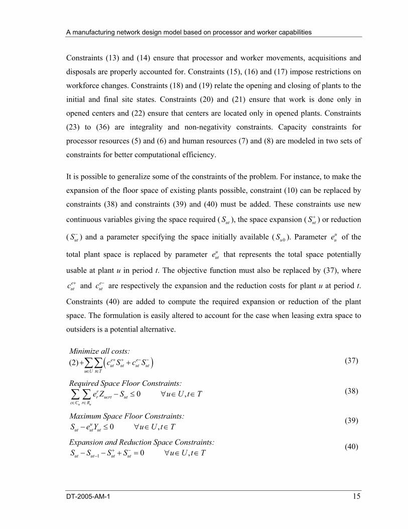
It is possible to generalize some of the constraints of the problem. For instance, to make the

expansion of the floor space of existing plants possible, constraint (10) can be replaced by

constraints (38) and constraints (39) and (40) must be added. These constraints use new

continuous variables giving the space required ( utS ), the space expansion ( utS + ) or reduction

( utS − ) and a parameter specifying the space initially available ( 0uS ). Parameter uue of the

total plant space is replaced by parameter uute that represents the total space potentially

usable at plant u in period t. The objective function must also be replaced by (37), where eutc + and e

utc − are respectively the expansion and the reduction costs for plant u at period t.

Constraints (40) are added to compute the required expansion or reduction of the plant

space. The formulation is easily altered to account for the case when leasing extra space to

outsiders is a potential alternative.

Minimize all costs: (2) ( )e e

ut ut ut utu U t T

c S c S+ + − −

∈ ∈

+ +∑∑ (37)

Required Space Floor Constraints: 0 ,

u u

rr ucrt ut

c C r Re Z S u U t T

∈ ∈

− ≤ ∀ ∈ ∈∑ ∑ (38)

Maximum Space Floor Constraints: 0 ,u

ut ut utS e Y u U t T− ≤ ∀ ∈ ∈ (39)

Expansion and Reduction Space Constraints: 1 0 ,ut ut ut utS S S S u U t T+ −−− − + = ∀ ∈ ∈

(40)


DT-2005-AM-1 16

To ensure a minimum activity level at a plant, constraints (41) can be added to the

formulation. The parameter utl represents the minimum activity level for the plant u in time

units in period t.

Minimum Plant Activity Level Constraints: 0 ,

up ucp ucrp

wrwpt ucwrpt ut ut

c C p M r R w Wh X l Y u U t T

∈ ∈ ∈ ∈

− ≥ ∀ ∈ ∈∑ ∑ ∑ ∑ (41)

To be more flexible, each plant could use a pool of mobile workers. In this case, some

workers are no longer assigned to specific centers in a plant. In order to achieve this type of

assignment, the number of mobile workers must be accounted for on a per plant basis,

which is done by adding constraint (42). The capacity provided by a mobile worker, muwtb , is

from a plant perspective, as well as the total number of required mobile workers, muwtH , and

the necessary overtime, mouwtH . These decision variables need to be added in the objective

function (2).

Mobile Worker Capacity Constraints: ( )ˆ 0

, ,u ucp u

w o m m moucwrpt ucwt ucwt ucwt uwt uwt uwt

c C p M r R c C

uc

H b H H b H H

u U w W t T∈ ∈ ∈ ∈

− + − − ≤

∀ ∈ ∈ ∈

∑ ∑ ∑ ∑ (42)

To take economies of scale and scope into account, processor types with distinct flexibility,

capacity and floor space requirements can be used. In extreme cases, it is also possible to

replace the processor concept used in this paper by the technology options concept

proposed by Paquet et al. (2004). Each of these technology options would correspond to a

specified number of processors with associated floor space requirements. Other

generalizations may be required for specific situations.

The model can be used to design a new manufacturing network, or to reengineer an existing

network, by examining different potential scenarios. These scenarios can be associated to

different demand patterns, different service policies, different sets of potential vendors,

different sets of potential manufacturing sites, etc. The model could also be used to guide

decisions on overtime rules in the context of a labor negotiation, on the introduction of new

products, on the opportunity to enter new markets, etc. Finally, it can be used to investigate


DT-2005-AM-1 17

potential threats, such as the restricted availability of specialized personnel on specific

labor markets.

3. Solution Method

With the power of modern commercial solvers, the first solution method to examine is the

proprietary branch and bounds algorithm that these solvers implement. Our mixed integer

programming (MIP) model can be directly implemented and solved with solvers like

CPLEX 9.0 (ILOG, 2003), which was used in our experiments. Commercial solvers can be

configured to automatically generate generic cuts to reduce computation times. For

example, CPLEX allows the generation of Gomory fractional cuts. Furthermore, our past

research (Paquet et al., 2004) showed that specific cuts can be derived to speed up the

resolution. The cuts proposed for the model presented here are related to capacity and are

defined by equations (43) to (45). A new parameter is required to describe these cuts: the

total network requirements for product-state p in period t ( ptx ). These requirements can be

derived from the deterministic demands pdtx . Cuts (43) and (44) calculate the minimum

number of processors and workers, respectively, required to satisfy total network demand.

Cuts (45) ensures that at least one center is used in the entire network for each

manufactured product-states.

Cuts Based on the Minimum Number of Processors: ˆ1 ,

p up ucp

r ucrpt ptrptu U c C r R

Z x p M t Th∈ ∈ ∈

≥ ∀ ∈ ∈∑ ∑ ∑ (43)

Cuts Based on the Minimum Number of Workers: ˆ1 ,

p up ucp ucrp

w ucwrpt ptrwptu U c C r R w W

H x p M t Th∈ ∈ ∈ ∈

≥ ∀ ∈ ∈∑ ∑ ∑ ∑ (44)

Cuts Based on the Minimum Number of Centers: 1 ,

p up

ucptu U c C

G p M t T∈ ∈

≥ ∀ ∈ ∈∑ ∑ (45)

These conceptually promising accelerative techniques were evaluated, in terms of

computational time reduction, through empirical experimentations. In most cases, these

techniques, when used with the default parameters of CPLEX, reduce the resolution time

slightly. For the experimental evaluations presented in the next section, in order to reduce


DT-2005-AM-1 18

computational times significantly for all cases, the following branch and bound CPLEX

parameter settings are used:

• CPX_PARAM_MIPEMPHASIS is set to CPX_MIPEMPHASIS_HIDDENFEAS, which instructs the solver to search high quality feasible solutions early in the optimization.

• CPX_PARAM_VARSEL is set to CPX_VARSEL_MAXINFEAS, which instructs the solver to branch on variable with maximum infeasibility.

• CPX_PARAM_BRDIR is set to CPX_BRDIR_UP, which instructs the solver to select the up branch first at each node of the branch and bound tree.

• CPX_PARAM_NODESEL is set to CPX_NODESEL_BESTEST, which instructs the solver to select the node with the best estimate of the integer objective value.

• CPX_PARAM_PROBE is set to 3, which is the maximum probing level on variables before branching.

For example, the computational time is decreased from 579 seconds with the default

settings to 195 seconds with these parameters for Scenario 1 discussed in the next section.

In what follows, the use of these CPLEX parameter values is referred to as optimal settings.

In order to obtain good solutions in an acceptable time for large problems, two additional

solver settings were used to reduce the number of branches explored in the branch and

bounds solutions tree:

• CPX_PARAM_OBJDIF is set to 500, which instructs the solver to select nodes that have a potential of decreasing the solution by at least 500 $.

• CPX_PARAM_EPGAP is set to 0.03, which instructs the solver to stop the resolution when the best node available has a potential of decreasing the solution by a maximum of 3% of the current best solution.

The problem is not solved to optimality when these parameter values are used and their

effect is discussed in the next section. In what follows, the use of these CPLEX parameter

values in addition to the optimal settings is referred to as near-optimal settings. The recent

technological progress of commercial solvers enables the efficient solution of more difficult

models. It is now possible to tackle realistic problems with commercial solvers and often to

solve them more efficiently than with specialized decomposition algorithms when

appropriate cuts are used (see Paquet et al. (2004) for a discussion on this topic). It is this

solution approach that is tested in this paper.


DT-2005-AM-1 19

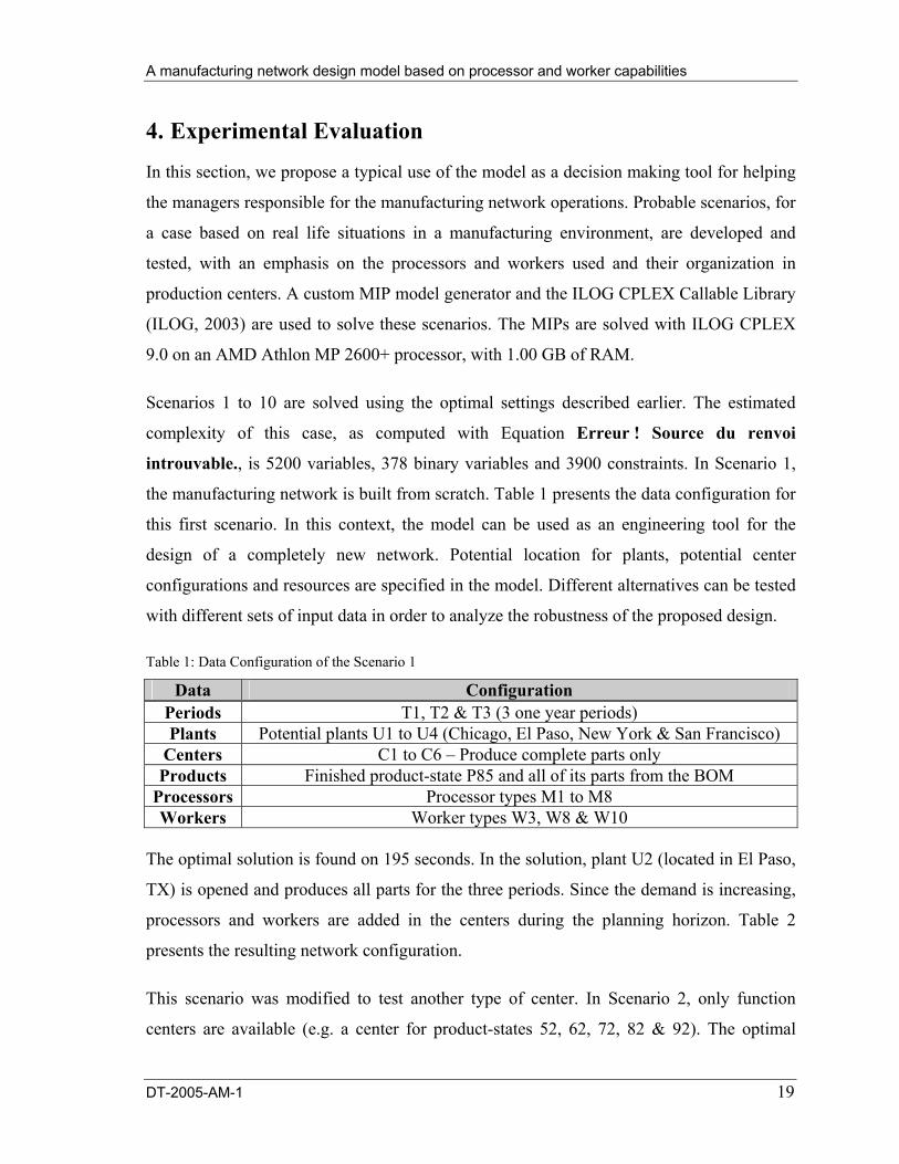
4. Experimental Evaluation

In this section, we propose a typical use of the model as a decision making tool for helping

the managers responsible for the manufacturing network operations. Probable scenarios, for

a case based on real life situations in a manufacturing environment, are developed and

tested, with an emphasis on the processors and workers used and their organization in

production centers. A custom MIP model generator and the ILOG CPLEX Callable Library

(ILOG, 2003) are used to solve these scenarios. The MIPs are solved with ILOG CPLEX

9.0 on an AMD Athlon MP 2600+ processor, with 1.00 GB of RAM.

Scenarios 1 to 10 are solved using the optimal settings described earlier. The estimated

complexity of this case, as computed with Equation Erreur ! Source du renvoi

introuvable., is 5200 variables, 378 binary variables and 3900 constraints. In Scenario 1,

the manufacturing network is built from scratch. Table 1 presents the data configuration for

this first scenario. In this context, the model can be used as an engineering tool for the

design of a completely new network. Potential location for plants, potential center

configurations and resources are specified in the model. Different alternatives can be tested

with different sets of input data in order to analyze the robustness of the proposed design.

Table 1: Data Configuration of the Scenario 1

Data Configuration Periods T1, T2 & T3 (3 one year periods) Plants Potential plants U1 to U4 (Chicago, El Paso, New York & San Francisco)

Centers C1 to C6 – Produce complete parts only Products Finished product-state P85 and all of its parts from the BOM

Processors Processor types M1 to M8 Workers Worker types W3, W8 & W10

The optimal solution is found on 195 seconds. In the solution, plant U2 (located in El Paso,

TX) is opened and produces all parts for the three periods. Since the demand is increasing,

processors and workers are added in the centers during the planning horizon. Table 2

presents the resulting network configuration.

This scenario was modified to test another type of center. In Scenario 2, only function

centers are available (e.g. a center for product-states 52, 62, 72, 82 & 92). The optimal


DT-2005-AM-1 20

solution is found in 21 seconds. The same plant is opened (El Paso, TX), 145 processors are

required for period 1 (+13 for period 2 & +18 for period 3) and 148 workers are required at

period 1 (+14 for period 2 & +19 for period 3). The total investment for this scenario is

36 769 066 $ (in present value). The resources needed for these two scenarios are

equivalent, but with a difference in the overall cost of more than 435 000 $.

Table 2: Optimal Network Configuration Based on Scenario 1

Data Period 1 Period 2 Period 3 El Paso C1 Activated Active Active El Paso C3 Activated Active Active El Paso C4 Activated Active Active Centers

El Paso C5 Activated Active Active El Paso M1 17 +1 +2 El Paso M2 41 +2 +5 El Paso M3 49 +5 +6 El Paso M4 5 +1 0 El Paso M5 7 0 0 El Paso M6 16 0 +4 El Paso M7 11 +3 0 El Paso M8 3 +1 0

Processors

Total 149 +13 +17 El Paso W3 34 +3 +4 El Paso W8 109 +8 +15 El Paso W10 3 +1 0 Workers

Total 146 +12 +19 Total Cost 36 332 558 $ (in present value) for 3 years

The first scenario has also been run with the complete set of developed centers in Scenario

3. The solution is found in 293 seconds at a cost of 36 102 756 $ (in present value). This is

a saving of 175 000 $ (compared with Scenario 1). As in the first two scenarios, El Paso,

TX, plant is opened. For this scenario, 147 processors are required in period 1 (+12 in

period 2 & +17 in period 3) and 144 workers are required for period 1 (+14 for period 2 &

+20 for period 3). A combination of product and function centers is selected. Table 3

compares these first three scenarios. These three scenarios show that this formulation can

be used to design manufacturing networks by selecting plants and suppliers of raw

materials, and by configuring the opened production plants. They also show that the


DT-2005-AM-1 21

organization of production centers has a significant effect on resource utilization, efficiency

and costs.

In Scenario 4 (3645 variables, including 216 binary variables, and 2607 constraints), the

addition of a new product (product-state P95) to the current manufacturing network

(Scenario 1) is analyzed. The demand forecast for the two finished products is optimistic in

this scenario, in particular for the new product P95 which has a very promising demand for

periods 2 and 3. The addition of this new product leads to the use of a second plant (Plant 3

– New York, NY) in the third year of the planning horizon. This scenario has a cost of

86 516 107 $ and the optimal solution is found in 144 seconds.

Table 3: Comparison of Scenarios 1, 2 & 3

Data Scenario 1 Scenario 2 Scenario 3 Plants Plant U2 (El Paso) Plant U2 (El Paso) Plant U2 (El Paso)

Centers Product centers only Function centers only All centers available Processors 149 + 13 + 17 = 179 145 + 13 + 17 = 175 147 + 12 + 18 = 176 Workers 146 + 12 + 19 = 177 148 + 13 + 18 = 179 144 + 14 + 20 = 178

Costs 36 332 558 $ 36 769 066 $ 36 102 756 $ Variables 4032 (276 bin. var.) 3672 (276 bin. var.) 5676 (588 bin. var.)

Constraints 2873 2513 4653 Time 195 s. 21 s. 293 s.

In Scenario 5 (5280 variables, including 345 binary variables, and 3487 constraints), a new

network is designed to make product P95 by considering a new set of potential plants (five

potential plants are used). This new network is completely independent of the network of

Scenario 1 in order to emulate a new enterprise. The solution leads to the opening of a plant

in Portland, OR. This plant is sufficient in space for the three years of the planning horizon.

This scenario has a cost of 49 404 443 $ and the solution is found in 185 seconds.

A new network for products P85 & P95 is build from scratch in Scenario 6 (16183

variables, including 1269 binary variables, and 9075 constraints). The complete sets of

plants and centers are used. Since we already know a solution for a subset of this problem

from Scenario 4, we use this information as MIP starts values in CPLEX to speed up the

resolution of this problem. This scenario has a cost of 87 702 458 $ and the solution is


DT-2005-AM-1 22

found in 620 seconds with the help of the starting solution. Without this technique, the

solution is found in 780 seconds.

The next three scenarios analyze resource capabilities (processors and workers). In these

scenarios, the manufacturing network obtained for Scenario 4 is used as the starting

network. A base scenario with no modification is built in order to obtain a comparison

point for these evaluations, over a three year planning horizon. For Scenario 7, a new

flexible processor (M11) is available on the market. The solution leads to a replacement of

the processors M3 by this new processor type. A saving of more than 5 000 000 $ over

three years can be achieved by using this new type of processor with the current capabilities

of the workers. For Scenario 8, a new flexible processor (M12) is available on the market,

but this time, new competencies are required for the workers to use it. If the enterprise

wants to use this processor type, workers of type W4 are also required. During the planning

horizon, processors of type M6 are replaced by processors of type M12 and workers of type

W3 are replaced by workers of type W4. This configuration leads to a saving of more than

5 500 000 $ over three years. For Scenario 9, the data of Scenario 8 is used as input, but

flexible workers W4 have limited availability. In this case, the cost related to this lack of

availability is 2 800 000 $ over three years (compared with Scenario 8). Table 4 shows the

comparison of these three scenarios related to the base scenario built from the resulting

manufacturing network of Scenario 4.

Table 4: Comparison of Scenarios 7, 8 & 9

Data Base (Scenario 4) Scenario 7 Scenario 8 Scenario 9 Processors M1 to M8 +M11 +M12 +M12 Workers W3, W8, W10 – +W4 +W4 (limited)

Costs 133,118,610 $ 127,280,403 $ 127,548,771 $ 130,141,467 $ Variables 2280 (135 bin.) 2442 (135 bin.) 2598 (135 bin.) 2598 (135 bin.)

Constraints 1950 2034 2049 2142 Time 3 s. 102 s. 54 s. 114 s.

Scenario 10 (3645 variables, including 216 binary variables, and 2469 constraints) is built

from Scenarios 1 (current network for product P85) and 5 (acquired network for product

P95), which emulate the acquisition of a plant and a reconfiguration of the current

manufacturing network. Initially, each plant produces one finished product. For this


DT-2005-AM-1 23

solution, each plant produces all finished products in the last period of the planning

horizon. This new configuration requires the rationalization of the resources during the

planning horizon (buy, sell, hire, layoff and transfer). At the end of the planning horizon the

second plant produces a main product-state (P43) for all plants and one or two finished

products for 35% of the clients. The complete solution costs is 107 891 842 $ and the

solution is found in 231 seconds (a saving of about 500 000 $ if Scenarios 1 & 5 are run

independently with the same demand). Table 5 presents the details of the solution. The

values between brackets represent resources transferred from (–) or to (+) a specific plant.

Table 5: Details of the Solution of Scenario 10

Plant U2 (El Paso, TX) Plant U6 (Portland, OR) Period Products Processors Workers Products Processors Workers

0 43, 63, 73, 85 & 95

179 177 43, 54, 73 & 95

334 328

1 43, 54, 63, 73, 85 & 95

427 [+246 (U6)]

423 43, 54, 73 & 95

66 [–246 (U2)]

63

2 43, 54, 63, 73, 85 & 95

433 [+6 (U6)]

426 43, 73, 85 & 95

76 [–6 (U2)]

66

3 43, 54, 63, 73, 85 & 95

434 [+3 (U6)]

430 43, 73, 85 & 95

74 [–3 (U2)]

68

Scenarios 11 to 25 were elaborated to test the model solution times for real size problems.

These scenarios were randomly generated using the data presented in Table 6. Each

scenario is generated with realistic data intervals for the customer demands of each period

of the planning horizon, and with the same initial state.

Table 6: Data Configuration of the Scenarios 11 to 25

Data Configuration Periods 3 one year periods

Suppliers 30 potential suppliers Plants 10 potential plants

Centers 30 potential centers for all plants (product centers, function centers, process centers & product group centers)

Demand Zones 189 demand zones corresponding to geographically aggregated customers locations

Products 6 finished product families and all of their parts (94 product-states) Processors 54 processor types Workers 38 worker types


DT-2005-AM-1 24

The problem size for these cases, as estimated with Equation Erreur ! Source du renvoi

introuvable., is 14058 variables, 930 binary variables and 10395 constraints. The exact

size of the problem generated is comprised between 14961 and 32559 continuous variables,

789 and 1398 binary variables and 11184 and 20967 constraints. The models to solve for

these scenarios are up to 10 time larger than for scenarios 1 to 10 (at least 3 times according

to the estimations of Equation Erreur ! Source du renvoi introuvable.). The near-optimal

settings were used to solve these ploblems. The potential network for these scenarios is

illustrated in Figure 6.

Figure 6: Potential Network for Scenarios 11 to 25

Figure 7 presents an example of solution quality and solution time for near-optimal,

optimal and default settings of the solver for Scenario 11. The problem to solve for this

scenario is composed of 26265 variables (1134 binary variables) and 15093 constraints.

The customized cuts permit to solve the linear relaxation of the problem in 9 seconds

compared of 18 seconds without the cuts. Since all nodes evaluated are solved faster, the

solution procedure is also faster. Note also that the starting lower bound with the

customized cut is higher by 1 690 000 $, which help for the proof of optimality. The

optimal solution is found with the customized parameter settings in more than 15000


DT-2005-AM-1 25

seconds. The default parameter solution was stopped after 12 hours of computation with a

current solution higher than the optimal cost by more than 2 600 000 $. The near-optimal

solution obtained in 874 seconds is less than 32 000 $ (0.03%) higher than the optimal

solution. Actually, it takes intensive computational efforts to prove that the near-optimal

solution is near the optimal cost. For these 15 scenarios, the solution time is between 454

and 3692 seconds and their solution quality is comprised between 0.01% and 0.81% of the

optimal cost.

Figure 7: Example of Solution Quality as a Function of Computational Time for Scenario 11

The 25 scenarios tested demonstrate the usefulness of the model as a design and what-if

analysis tool for the planning of a manufacturing network with explicit consideration of

resources. Some of these scenarios are difficult to solve to optimality with the solver

default settings. In fact, the optimal solution is often found after a short amount of time.

However, it takes a lot more time to prove that it is optimal, as shown in Figure 7. In order

to reduce this time, a better lower bound must be found for the problem. To achieve this,

custom cuts have been developed and customized solver settings were used. It is also


DT-2005-AM-1 26

possible to reduce the solution time by finding a better upper bound, that is, a good start-up

solution, using information obtained from previous scenarios (see Scenario 6 for an

example).

5. Conclusion

This paper has introduced a multi-period optimization model and a methodology to design

networks of manufacturing facilities producing several products under deterministic

demand. The approach can deal with the manufacturing operations required for each

product, as well as the availability and mobility of manufacturing resources, in multiple

production center plants. The operations for each product are taken into account by

incorporating product-state graphs in the model. Worker competencies, overtime and

processor flexibility are also taken into account. Computational results show that the

proposed model can be solved efficiently with commercial mixed-integer programming

solvers by adding appropriate cuts to the original model. Future work related to this

problem concerns the integration of the order-to-delivery time and the service level in the

methodology of manufacturing network design. These factors must be taken into account in

order to capture the variation of the demand and its effect on the capacity required.

6. References

Arntzen, B.C., G.G. Brown, T.P. Harrison and L.L. Trafton (1995) Global Supply Chain Management at Digital Equipment Corporation. Interfaces 25(1), 69-93.

Benjaafar, S. and D. Gupta (1998) Scope Versus Focus: Issues of Flexibility, Capacity, and Number of Production Facilities. IIE Transactions 30(5), 413-425.

Benjaafar, S. and M. Sheikhzadeh (2000) Design of Flexible Plant Layouts. IIE Transactions 32(4), 309-322.

Cohen, M.A., M. Fisher and R. Jaikumar (1989) International Manufacturing and Distribution Networks: A Normative Model Framework. In: Managing International Manufacturing, Kasra Ferdows (ed), 67-93, Amsterdam: Elsevier Science Publishers.

Cohen, M.A. and S. Moon (1991) An Integrated Plant Loading Model with Economies of Scale and Scope. European Journal of Operational Research 50(3), 266-279.

Cohen, M.A. and S. Moon (1990) Impact of Production Scale Economies, Manufacturing Complexity, and Transportation Costs on Supply Chain Facility Networks. Journal of Manufacturing and Operation Management 3, 269-292.


DT-2005-AM-1 27

Cordeau, J.-F., F. Pasin and M.M. Solomon (2002) An Integrated Model for Logistics Network Design. Les Cahiers du GERAD G–2002–07, 30 p.

Dogan, K. and M. Goetschalckx (1999) A Primal Decomposition Method for the Integrated Design of Multi-Period Production-Distribution Systems. IIE Transactions 31(11), 1027-1036.

Geoffrion, A.M. and R.F. Powers (1995) Twenty Years of Strategic Distribution System Design: An Evolutionary Perspective. Interfaces 25(5), 105-127.

ILOG (2003) ILOG CPLEX 9.0 User's Manual.

Lakhal, S., A. Martel, O. Kettani and M. Oral (2001) On the Optimization of Supply Chain Networking Decisions. European Journal of Operational Research 129(2), 259-270.

Martel, A. (2005) The Design of Production-Distribution Networks: A Mathematical Programming Approach. In: Supply Chain Optimization, Geunes, J. and Pardalos, P. (eds), Kluwer Academic Publishers.

Mazzola, J. and R. Schantz (1997) Multiple-Facility Loading Under Capacity-Based Economies of Scope. Naval Research Logistics 44, 229-256.

Montreuil, B. and P. Lefrançois (1996) Organizing Factories as Responsability Networks. In: Progress in Material Handling Research: 1996, Robert Graves et al. (eds), 36 p., Ann Arbor, Michigan, U.S.A.: Material Handling Institute, Braum-Brumfield inc.

Montreuil, B., Y. Thibault and M. Paquet (1998) Dynamic Network Factory Planning and Design. In: Progress in Material Handling Research: 1998, Robert Graves et al. (eds), 353-380, Ann Arbor, Michigan, U.S.A.: Material Handling Institute, Braum-Brumfield inc.

Paquet, M., A. Martel and G. Desaulniers (2004) Including Technology Selection Decisions in Manufacturing Network Design Models. International Journal of Computer Integrated Manufacturing 17(2), 117-125.

Revelle, C.S. and G. Laporte (1996) The Plant Location Problem: New Models and Research Prospects. Operations Research 44(6), 864-874.

Shapiro, J.F. (2001) Modeling The Supply Chain. 586 p. Duxbury.

Vercellis, C. (1991) Multi-Criteria Models for Capacity Analysis and Aggregate Planning in Manufacturing Systems. International Journal of Production Economics 23(1-3), 261-272.

Verter, V. and A. Dasci (2002) The Plant Location and Flexible Technology Acquisition Problem . European Journal of Operational Research 136(2), 366-382.

Verter, V. and M.C. Dincer (1992) An Integrated Evaluation of Facility Location, Capacity Acquisition, and Technology Selection for Designing Global Manufacturing Strategies. European Journal of Operational Research 60(1), 1-18.

Vonderembse, M.A. and M. Tracey (1999) The Impact of Supplier Selection Criteria and Supplier Involvement on Manufacturing Performance. Journal of Supply Chain Management 35(3), 33-39.

Date post:	15-Mar-2022
Category:	Documents
Upload:	others
View:	2 times
Download:	0 times

A manufacturing network design model based on processor ...

Documents