A Programmable Architecture for Real-time Derivative Trading

A Programmable Architecture for Real-time

Derivative Trading

Sachin TandonT

HE

U N I V E RS

IT

Y

OF

ED I N B U

RG

H

Master of Science

Computer Science

School of Informatics

University of Edinburgh

2003

Abstract

Derivatives are financial securities that are used to hedge business risks, caused by

changes in foreign exchange rates, interest rates or prices of goods. The algorithms in

the models used to analyse such derivatives often cannot handle the real-time process-

ing of large volumes of financial data in a pure software environment.

This thesis aims to document the investigation into the implementation of such models

onto a Xilinx Virtex-II Pro architecture, which consists of an embedded processor and

an FPGA. The project explores the partitioning of the software algorithm over the two

components in this architecture, so as to be capable of processing the financial data in

real-time.

The thesis looks at the implementation of progressively computationally intensive al-

gorithms of this architecture, and the results and conclusions drawn from the experi-

ments. It also highlights the problems faced in this context, along with future work to

remedy these issues. It finds that the financial algorithms are suitable for processing

on this platform, and performance would be greatly enhanced.

i

Acknowledgements

I would like to first and foremost thank my supervisors, Christopher von Mecklenburg

and D.K. Arvind for their guidance, support and patience throughout the course of

the project. A special thanks also to Janek Mann, who devoted a lot of his valuable

time to answering my many questions, and for sharing his Partitioner software. I am

grateful towards Olsen Ltd. for their support, by providing their proprietary software

and historical data.

I would also like to thank Mathematica and UnRisk for providing evaluation copies of

their software for this project. A special thanks also to Reliance Industries Ltd., for the

opportunity to do an ethnographic study of their derivatives trading room.

The experiments were performed using software from Xilinx, Symphony, ARM and

Mathematica. WinEdt and MiKTeX were used for typesetting this document.

ii

Declaration

I declare that this thesis was composed by myself, that the work contained herein is

my own except where explicitly stated otherwise in the text, and that this work has not

been submitted for any other degree or professional qualification except as specified.

(Sachin Tandon)

iii

Table of Contents

1 Introduction 1

1.1 Thesis organisation . . . . . . . . . . . . . . . . . . . . . . . . . . . 2

2 Theory and Background 4

2.1 Derivatives . . . . . . . . . . . . . . . . . . . . . . . . . . . . . . . 4

2.1.1 Definition . . . . . . . . . . . . . . . . . . . . . . . . . . . . 4

2.1.2 Categorisation of derivatives . . . . . . . . . . . . . . . . . . 4

2.1.3 Common derivatives . . . . . . . . . . . . . . . . . . . . . . 6

2.2 Soft-Hardware computation . . . . . . . . . . . . . . . . . . . . . . . 9

2.2.1 Embedded Computation . . . . . . . . . . . . . . . . . . . . 9

2.2.2 Reconfigurable logic . . . . . . . . . . . . . . . . . . . . . . 11

2.2.3 Mixed environment . . . . . . . . . . . . . . . . . . . . . . . 14

3 Preliminary Analysis and Design 16

3.1 Project Architecture . . . . . . . . . . . . . . . . . . . . . . . . . . . 16

3.1.1 Computation Engine . . . . . . . . . . . . . . . . . . . . . . 17

3.1.2 Wireless Transceivers . . . . . . . . . . . . . . . . . . . . . . 18

3.1.3 The Data Filter . . . . . . . . . . . . . . . . . . . . . . . . . 18

3.2 Architecture considerations . . . . . . . . . . . . . . . . . . . . . . . 19

3.2.1 Processor selection . . . . . . . . . . . . . . . . . . . . . . . 20

3.2.2 FPGA design methodology . . . . . . . . . . . . . . . . . . . 21

4 Interest-Rate based Computations 24

4.1 OANDA’s financial model . . . . . . . . . . . . . . . . . . . . . . . 24

4.1.1 Service Model . . . . . . . . . . . . . . . . . . . . . . . . . 24

4.1.2 Applicability to this project . . . . . . . . . . . . . . . . . . 25

4.1.3 Interest Calculation Algorithms . . . . . . . . . . . . . . . . 25

4.1.4 Implementation . . . . . . . . . . . . . . . . . . . . . . . . . 26

iv

4.2 The Greeks . . . . . . . . . . . . . . . . . . . . . . . . . . . . . . . 28

4.2.1 Volatility Background . . . . . . . . . . . . . . . . . . . . . 29

4.2.2 The different Greeks . . . . . . . . . . . . . . . . . . . . . . 29

4.2.3 The Delta . . . . . . . . . . . . . . . . . . . . . . . . . . . . 30

4.2.4 Implementation . . . . . . . . . . . . . . . . . . . . . . . . . 31

5 Option Pricing 35

5.1 Black-Scholes Option Pricing . . . . . . . . . . . . . . . . . . . . . . 35

5.2 Standard Normal Distribution . . . . . . . . . . . . . . . . . . . . . . 37

5.2.1 The Erf function . . . . . . . . . . . . . . . . . . . . . . . . 37

5.3 Reference computation . . . . . . . . . . . . . . . . . . . . . . . . . 39

5.3.1 Reference standard normal distribution . . . . . . . . . . . . 39

5.4 Implementation . . . . . . . . . . . . . . . . . . . . . . . . . . . . . 40

5.4.1 FPGA Implementation . . . . . . . . . . . . . . . . . . . . . 40

5.4.2 ARM implementation . . . . . . . . . . . . . . . . . . . . . 42

5.4.3 Results . . . . . . . . . . . . . . . . . . . . . . . . . . . . . 42

6 Analysis and Conclusions 48

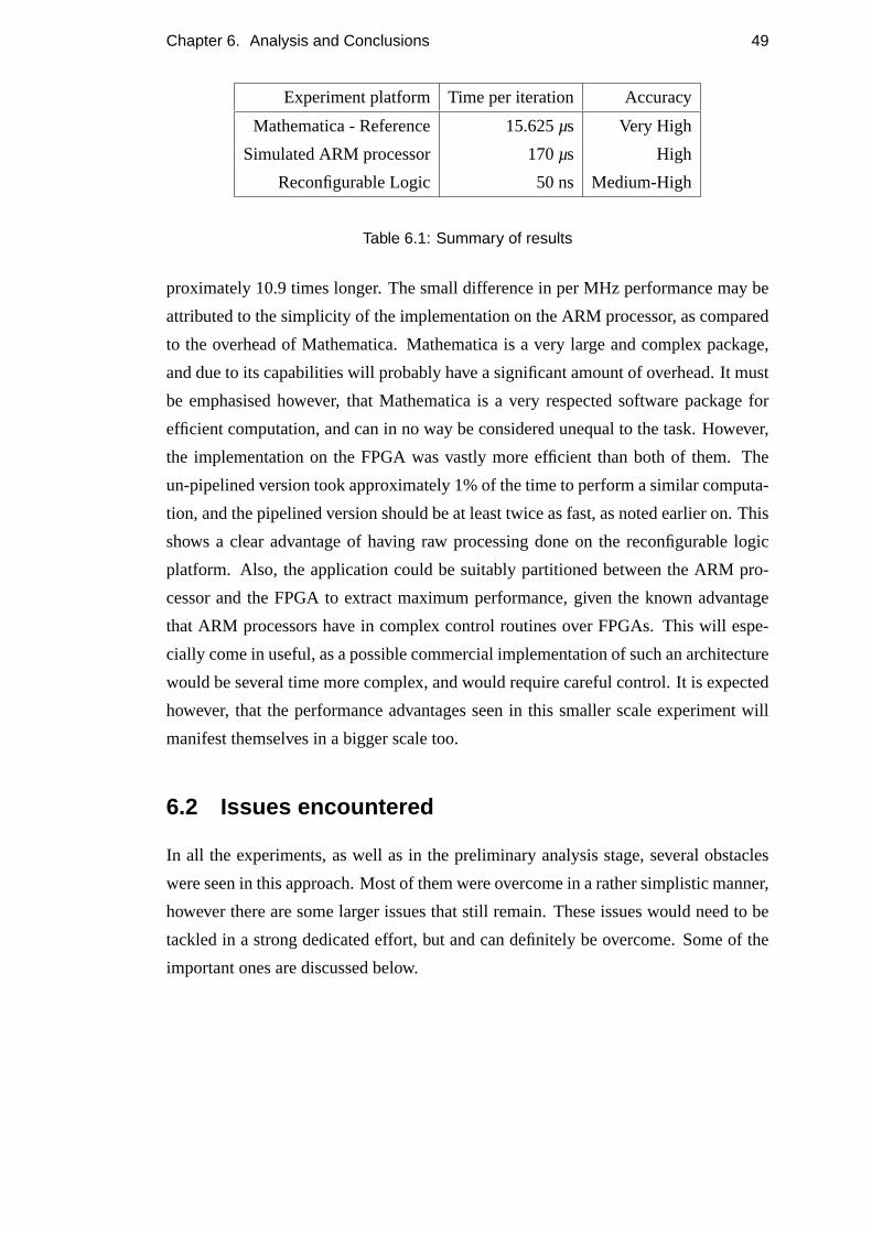
6.1 Evaluation of results . . . . . . . . . . . . . . . . . . . . . . . . . . 48

6.1.1 Option Pricing experiment results . . . . . . . . . . . . . . . 48

6.2 Issues encountered . . . . . . . . . . . . . . . . . . . . . . . . . . . 49

6.2.1 Floating-Point computations . . . . . . . . . . . . . . . . . . 50

6.2.2 Data acquisition . . . . . . . . . . . . . . . . . . . . . . . . 51

6.2.3 Mathematical infrastructure for computation . . . . . . . . . 51

6.3 Conclusions . . . . . . . . . . . . . . . . . . . . . . . . . . . . . . . 52

6.3.1 Feasibility of approach . . . . . . . . . . . . . . . . . . . . . 52

6.3.2 Benefits of approach . . . . . . . . . . . . . . . . . . . . . . 53

6.4 Future Work . . . . . . . . . . . . . . . . . . . . . . . . . . . . . . . 54

6.4.1 Fixed-Point Computation . . . . . . . . . . . . . . . . . . . . 54

6.4.2 Mathematical Infrastructure . . . . . . . . . . . . . . . . . . 55

6.4.3 Hull-White model . . . . . . . . . . . . . . . . . . . . . . . 55

A Reference Black-Scholes implementation 56

B Output run from OANDA implementation 58

Bibliography 60

v

List of Figures

2.1 Linear Derivative . . . . . . . . . . . . . . . . . . . . . . . . . . . . 5

2.2 Convex Derivative . . . . . . . . . . . . . . . . . . . . . . . . . . . . 5

2.3 Concave Derivative . . . . . . . . . . . . . . . . . . . . . . . . . . . 5

2.4 Mixed Derivative . . . . . . . . . . . . . . . . . . . . . . . . . . . . 5

2.5 Generic FPGA Layout . . . . . . . . . . . . . . . . . . . . . . . . . 13

3.1 Project Architecture . . . . . . . . . . . . . . . . . . . . . . . . . . . 17

3.2 FPGA Design Flow . . . . . . . . . . . . . . . . . . . . . . . . . . . 23

5.1 PDF of the Standard Normal Distribution . . . . . . . . . . . . . . . 38

5.2 CDF of the Standard Normal Distribution . . . . . . . . . . . . . . . 38

5.3 Mathematica : Black-Scholes verification . . . . . . . . . . . . . . . 44

5.4 ARM Processor : Black-Scholes verification . . . . . . . . . . . . . . 44

vi

Chapter 1

Introduction

Today, a very important part of the burgeoning financial markets is the trading of

derivative securities. These financial instruments are high risk investments that are

devices for transferring risk. The biggest market that derivative securities are involved

in is the foreign exchange market, although commodity markets are no stranger to

these instruments. Apart from being very risky, the models and tools used to analyse

derivatives are extremely complicated. Also, their volume of trading in the financial

markets result in the generation of large volumes of numerical data, such as prices of

derivatives, related interest rates, foreign exchange rates etc. The algorithms thus used

in these analysis models have to deal with these large amounts of data, and are compu-

tationally very intensive. For some of these algorithms, a fully software based solution

will not be able to handle the processing of data in real time.

This project has aimed to look into the implementation of these algorithms on a mixed

software-hardware platform. The architecture used was based on the Xilinx Virtex-II

Pro platform, which consists of a FPGA and an embedded processor. The said financial

algorithms can be partitioned across the processor and the FPGA, and thus will be able

to analyse the market data in real time to deliver maximum strategic knowledge to the

investor. Initially the project has looked into the feasibility of this approach, and the

benefits achieved by it. After this, the project looked into the implementation of some

of the algorithms onto such an architecture, starting initially with simple algorithms

and progressing to more computationally intensive ones.

1

Chapter 1. Introduction 2

1.1 Thesis organisation

In Chapter 2, the thesis outlines some of the background information about derivative

securities, and provides an introduction to some of the common derivatives with ex-

amples. It then goes on to highlight the target architecture and its components, for

implementation of the financial algorithms. It gives a brief introduction to embedded

computation for the processor portion of the architecture, and reconfigurable logic for

the FPGA portion.

Chapter 3 details the broad project design that is being envisioned. It consists of a

model where raw data is received from a market data source, filtered to remove anoma-

lies, and then run through a computation engine where the financial algorithms process

this data. The results of this computational analysis are then distributed to the end user

investors. While keeping the project vision in mind, the work done here has focused

on the computation engine specifically. This chapter also talks about the design deci-

sions that were made for this project regarding the specifics of the architecture and the

reasons for them.

Chapter 4 looks at the first two experiments that were conducted during the course of

the project. The first experiment tries to replicate a part of the FXTrade online service

by OANDA. It concerns a trading service where interest is both charged and paid to the

subscribers of the service, based on their investments in the foreign exchange market.

This is a mostly lightweight computation with regards to the architecture, and is thus

implemented on only the processor portion of the target architecture. The second ex-

periment has a greater requirement of computational power, and is partitioned across

both the processer and the FPGA. This experiment looks at a set of analysis tools for

derivatives called the Greeks, and the implementation of one of them, the Delta. These

analytical tools are values that are a measure of the sensitivity of a particular derivative,

and are very helpful to traders in deciding their strategy.

In Chapter 5, a third experiment is conducted, which is rather computationally inten-

sive. This experiment looks at some aspects of the theory and implementation of the

Black-Scholes option pricing model, which is used to compute the fair value price of

a special type of derivative called an option. A paper by S. Benninga and Z. Wiener

[Benninga and Wiener, 1997b] contains an implementation of this model in the Math-

ematica environment, which is taken as a reference point. Similar implementations are

done on two independent platforms, an embedded processor and an FPGA. This exper-

iment is an attempt to show the superiority of the FPGA for such purposes, by pitting

Chapter 1. Introduction 3

it against an embedded processor environment, and a more complex, general-purpose

processor environment, i.e. Mathematica. Tests are then conducted to show the perfor-

mance of the three platforms for this particular model, and the results are presented.

In the final chapter, an evaluation of the results of the third experiment are shown, fol-

lowed by a discussion into three of the issues and problems faced during the course

of this project. They are the issue of support of floating-point computation in pro-

grammable hardware, the problem of data acquisition and the need for a mathemat-

ical library of computational functions which can fulfill the needs of most financial

algorithms. The broad and qualitative conclusions of the project are also presented,

specifically looking at the feasibility and the benefits of this project. These reflect that

this project is a positive approach in the right direction, and financial traders may well

benefit significantly if their analytical tools are implemented on a platform such as the

one proposed. An insight is also provided into future directions that may be inves-

tigated following the results of this project. These directions include rectification of

the obstacles faced in this project and investigation into the implementation of more

complex algorithms.

Chapter 2

Theory and Background

2.1 Derivatives

2.1.1 Definition

A derivative is a financial contract whose value is derived from the value of another as-

set, called an underlying asset. A derivative may also be defined as a financial security,

just as stocks, debts and other equity assets are.

2.1.2 Categorisation of derivatives

Although it is possible to group derivatives in several different ways, the most lucid

approach is to categorise them them intolinear andnon-linearcategories. The differ-

ence between the two is in how the payoff function of the derivative is, as related to

the value of the underlying asset.

2.1.2.1 Linear derivatives

Linear derivatives are ones in which the payoff function is a linear function (Figure

2.1). The payoff for this kind of a derivative does not change with time and space, and

is fixed for every tick movement in the markets. It is easy to hedge (Section 2.1.3.1)

and one can be completely locked into the contract.

A derivative security will be locally linear if, between asset pricesS1 and S2, and

0 < λ < 1, the following equality is satisfied :

V(λS1 +(1−λ)S2) = λV(S1)+(1−λ)V(S2) (2.1)

4

Chapter 2. Theory and Background 5

Underlying Asset

Derivative Price

Figure 2.1: Linear Derivative

Underlying Asset

Derivative Price

Figure 2.2: Convex Derivative

2.1.2.2 Non-Linear derivatives

In non-linear derivatives, the payoff function changes with space and time and is thus

non-linear. It is possible for the function to follow a convex (Figure 2.2), concave

(Figure 2.3) or a mixed path (Figure 2.4) too. Generally speaking, for asset pricesS1

andS2, with 0 < λ < 1, the derivative function will be convex betweenS1 andS2 if:

V(λS1 +(1−λ)S2)≤ λV(S1)+(1−λ)V(S2) (2.2)

and concave if:

V(λS1 +(1−λ)S2)≥ λV(S1)+(1−λ)V(S2) (2.3)

Underlying Asset

Derivative Price

Figure 2.3: Concave Derivative

Underlying Asset

Derivative Price

Figure 2.4: Mixed Derivative


2.1.3 Common derivatives

Derivatives are a very import part of the international trading markets. The first deriva-

tive market was in the mid-1800s in Chicago, U.S.A where a futures market was

formed. Derivative securities today range from simplerfuturesandforwards, to more

exoticoptions, with a wide range in between. Futures and forwards are generally put in

the same category of derivatives because of a seemingly similar structure, but in reality

there are big differences in the way that deals involving them are executed. This re-

sults in them having different risks associated with them, and being accorded different

levels of flexibility. They are both linear derivatives, whereas options are non-linear

derivatives.

2.1.3.1 Forwards

A forward is anOver-The-Counter(OTC) contract, which specifies an obligation to

buy or sell a financial instrument or to make a payment at some point of time in the

future. An obligation to make a delivery in a forward is called as being theshort

position, and an obligation to accept a delivery in a forward is called as being in the

long position.

The terms of this agreement are dictated by the actual contract, which include the

date of the forward transaction and the place where it shall take place, among others.

These details are settled privately between the concerned parties. Also, being an OTC

contract, it is traded through a broker, and not an exchange. The two parties agree to

assume the credit risk of the other, and may, but are not required to set aside some

collateral in case of default, as is usually the case. If one of the parties wishes to

withdraw from the contract, it is at the mercy of the other party.

The important point to note about a forward contract is that it is neither an asset or a

liability for either of the parties involved, simply an agreement. Thus, itsMark-To-

Marketvalue at the time of inception is zero. Forward contracts are also generally not

traded in a secondary market.

Forwards Example : Hedging A firm in Europe owes an American company US$

1,000,000 after a time period of 6 months. Their home currency is the Euro, and

it is possible that 6 months later the Euro would have dropped with respect to the

US$, and they might pay more than they were planning to. Thus, they canhedge

the risk with another party, such as a bank to provide them with US$ 1,000,000

after 6 months in return for a fixed amount of Euros, which is decided today.


Thus the firm pays a little bit extra today, as insurance against major losses due

to foreign exchange fluctuations later on. The bank is expecting the Euro to rise

in the next 6 months, and thus takes on this risk on itself.

2.1.3.2 Futures

A future is an exchange-traded contract, which specifies an obligation to buy or sell

a commodity such as a financial instrument or to make a payment on a fixed delivery

date in the exchange. The details of the future contract are available publicly to the

exchange and settlement of the contract takes place through the exchange itself. This

is in contrast to the forward contract, in which this part of the transaction takes place

Over-The-Counter, in private. Because of this method of dealing, the terms in futures

contracts are generally standardised which are:

• Quantity of the underlying asset

• Quality of the underlying asset (Required only for non-financial assets)

• Date of delivery

• Units of price quotation, and tick-size

• Location of transaction

Since futures contracts are traded on the exchange, they have greater liquidity as

compared to forwards and therefore have a lower measure of risk. In the futures mar-

ket, the clearing house or the exchange is a counter-party to every trade, thus trans-

ferring the credit risk to the exchange, rather than on individual parties. Thus the risk

of default in trading is almost nil. Also, futures are more liquid, because of standard-

ised reporting of volumes and prices. Furthermore, if a party wishes to back out of a

contract, a futures contract can be reversed with anyone in the exchange. Commonly

traded futures include commodities (agricultural or otherwise), foreign exchange, stock

indices, interest rates etc.

Futures Example While trading in the foreign exchange futures market (which is the

biggest futures market), a firm enters into a futures contract to receive X units

of the US$ at a fixed price, 6 months later on by paying Y units of the British

pound. Thus the firm is in along position. Since this is traded on an exchange,

a cash settlement is done at the end of every trading day for the change in ex-

change rates. Sometime later, the firm may choose to goshort, by entering into


a contract to deliver X units of the US$ at the same day as the previous contract

for a higher price. Thus the firm has a guaranteed profit of the price difference

between the new and the old contract.

2.1.3.3 Options

An option is an agreement between two parties, that gives one of the parties the right,

but not the obligation to buy or sell an asset at a specified date (or during a specified

time frame) at a pre-determined price. If the option is not exercised within the stipu-

lated time-period, it simply expires and reduces its value reduces to zero. The price of

the option is called thestrike price, and the date of expiration of the option is called

thematurity dateor simply, theexpiry date. As a price for having the option, but not

the compulsion to perform the transaction, the option holder usually pays apremiumto

the option issuer. There are different styles of the option contract, which dictate when

the option can be exercised. A European style option can only be exercised on the

pre-decided maturity date, whereas an American style option can be exercised at any

given date before the maturity, and after the agreement. As a middle-path, a Bermudan

style option can be exercised on specific days between the agreement and the maturity

date. There are two basic type of option agreements, acall option and aput option.

• Call - A call gives the option holder the right, but not the obligation to buy an

asset as per the terms of the option. In a call, the buyer has the right to cancel

the option, or let it expire.

• Put - A put gives the option holder the right, but not the obligation to sell an

asset as per the terms of the option. In a put, the seller has the right to cancel the

option, or let it expire.

Options Example : Real-estateIn the real-estate market, a prospective buyer X wishes

to make money by dealing on properties. X then approaches the owner Y of

a particular property item, and purchases the option to buy the property af-

ter 6 months for US$100,000, and pays US$10,000 to Y for this right. Thus

US$100,000 is the decided price, and US$10,000 is the premium paid. If at the

end of 6 months, property prices rise, and X feels he can sell that property for a

price greater than the decided price of US$100,000, he/she decides to exercise

the option and pays Y the decided price and acquires the property. However, if

at the end of 6 months, property prices fall, and X feels that the property would


be a losing proposition, he/she lets the option expire and Y keeps the initial pre-

mium paid of US$10,000. This is a European style option, and were the option

such that X could purchase the property at any time in those 6 months, it would

have been an American style option.

2.2 Soft-Hardware computation

Traditionally, most applications that require any form of computation have been using a

pure software environment for processing, or have resorted to a hardware environment,

such as dedicated logic. The exception have been applications which are meant to be

extremely dependable, yet are extremely complex, such as avionic systems, as they

form a blend of both. In an area like financial computation, given the complexity of

data involved, and the desired approximate results, software based computation has

always been preferred, as it was not worth investing heavily inApplication Specific

Integrated Circuits(ASICs) or similar computational methods.

In this project, I propose the usage ofsoft-hardware computation, which is essentially

a balanced mixture of a software environment for processing of information and to

function as a control system, with a hardware/reconfigurable logic environment for

core processing of data. For this purpose, I wish to talk about two specific forms of

computation that I have been involved with in this project.

2.2.1 Embedded Computation

Embedded computation takes place in an embedded system, which is usually aspecial-

purposecomputer targeted to meet specific requirements. However, the lines are a

little blurry today, with the advent of more powerful computers and architectures, thus

resulting in more general-purpose computers being reduced to perform as an embedded

system. Thus we have general-purpose CPUs being used for this form of computation,

such as the ones mentioned in Section 2.2.1.2.

2.2.1.1 Benefits

The primary benefit of using an embedded system for computation for specialised ap-

plications is that almost all of the unnecessary functionality of the system is removed.

This itself gives rise to several benefits, some of which are briefly listed below.


Computational efficiency Eliminating non-essential functionality can lead to faster

computation simply by eliminating series of function calls, unnecessary valida-

tion code etc. Since an embedded system is constrained by its resources, it often

can be designed to handle very specific situations, and ignore all others. This

gives the ability of the Operating System or the application involved to behave

as a soft or hard real-time system. For example, it may be be possible to execute

some code directly within kernel space in aReal-Time Operating System(RTOS)

as it can be assumed to be safe, and thus skip some of the bounds checking done

in the user-space portion of the kernel, and the stacking of function calls to ex-

ecute the privileged portions of the code in kernel space. This however, does

lead to the problem of RTOS’s not being as scalable to more powerful embedded

architectures or to more complex functionality sometimes desired. However, an

added benefit of this is the cost of the designed system, as processors with much

lower computational power can be used. Today, the processors in the embedded

systems can be up to one-tenth the clock speed of their counterparts in general-

purpose computers.

Small stack sizeThe eliminating of functionality from the OS or the stack leads to

a much smaller executable size, thus allowing it to fit within the constrained

resources. For example, a specialised embedded software system for an avionics

component will probably not have any use for specific I/O technologies like USB

and IEEE 1394, nor would it used networking technologies like Ethernet. The

code size reduction from the removal of driver code alone from these systems is

significant. Similarly, some systems do not need code to handle file-systems, or

graphical user interfaces, which can all be removed. This too benefits the cost of

the designed system, as much lower resources in terms of primary and secondary

memory may be required. Some of the cost thus reduced is the manufacturing

cost, as the bill of materials value will drop down.

Lower rate of errors Humphrey [Humphrey, 1995] says that an experience software

engineer injects about 100 defects in every KLOC (Thousand Lines of Code).

This is a rather high rate of errors, and extensiveverification and validationis

required for the removal of these errors. Products still usually ship with some

errors, as it is very hard to make software that is a hundred percent correct, even

when methodologies like Cleanroom Software Engineering are used. Method-

ologies like that are often extremely costly to follow in both monitory and tem-


poral terms. However, embedded systems are designed for high reliability and

and must be very close to being error free. Removing unnecessary functional-

ity from a system often reduces the code size substantially, and thus lowers the

number of errors injected into the system. Also the smaller code size can be

more easily verified and validated, removing a larger percentage of errors during

that process. Thus the resultant system is highly reliable in most circumstances.

2.2.1.2 Architectures

Some of the architectures that are common for embedded computation today are briefly

described below.

PowerPC The PowerPC architecture was formed by IBM, Motorola and Apple as part

of the PowerPC alliance. The processors are designed asReduced Instruction

Set Computing(RISC) processors, as compared to the x86 desktop architecture

used by Intel which areComplex Instruction Set ComputingCISC processors.

The PowerPC 405 CPUs are very popular in the embedded segment, although

several other products are also available. The PowerPC architecture (with some

additional enhancements) is also used on the general-purpose platform for com-

puters by companies such as Apple and IBM.

ARM The ARM architecture is developed by ARM Ltd. which makes both 16 and 32

bit RISC microprocessors. The architecture is very ideal for embedded compu-

tation and a variety of extensions are available for specialised on-chip process-

ing such as Jazelle enhancements for Java, and audioDigital Signal Processing

(DSP) purposes. A variant of this architecture by Digital, called StrongARM has

been extended in collaboration with Intel to provide the XScale processors for

hand-held and other embedded devices.

MIPS MIPS has been the industry standard for a long time, and provides for high-

performance 32 and 64 bit architectures for embedded (and general-purpose)

computing. It is widely used in network processors (Cisco), gaming consoles

(Nintendo), cable set-top boxes, printers and smart cards among other devices.

2.2.2 Reconfigurable logic

Hardware based systems traditionally are several times faster than a pure software, or

embedded system. These systems are hand-designed to give optimum performance at


the hardware level, however, designing applications on hardware is extremely time-

consuming and quite difficult. The answer to this has been reconfigurable logic, en-

abled by the use of aField Programmable Device(FPD). There are various types of

FPDs, ranging from a simple Programmable Logic Array (PLA), to a more complex

type like aComplex Programmable Logic Device(CPLD) and aField Programmable

Gate Array(FPGA). FPGAs are generally used for more complex applications than

their closest counterparts, the CPLDs. A CPLD provides wider logic resources (more

AND planes), but a lower ratio of flip-flops to logic resources [Brown and Rose, 1996].

An important technology that allowed for the development of FPDs was the various

different types of switch technologies. Today, CPLDs use either anErasable Pro-

grammable Read-Only Memory(EPROM) or anElectrically Erasable Programmable

Read-Only Memory(EEPROM), while FPGAs useStatic Random Access Memory

(SRAM) andantifusetechnologies. SRAM is a CMOS technology, and it is volatile,

whereas antifuse is a CMOS+ technology which is non-volatile, but is not repro-

grammable (write once only). An FPGA primarily consists of logical units(Logic

blocks), and Input/Output Units (I/O Blocks) and interconnects. An diagram show-

ing the layout of a generic FPGA is as shown in Figure 2.5.

2.2.2.1 Benefits

Reconfigurable logic has one main disadvantage as compared to a pure-software envi-

ronment for computation, which is that it is generally a little harder and more expensive

to design and implement, even though the design cycle is simpler than an ASICs design

cycle. Advancements have been made in this field, and most problems have been over-

come. The advantages however, of reconfigurable logic over a microprocessor based

computation environment are many, according to [Hwu, 2003]. Some of them are

Spacial vs. Temporal Computation In a software environment, where computation

is done in a general-purpose CPU or an embedded CPU, all processing is tem-

poral, or more specifically,serial. Thus, only one computation can proceed at

a time, resulting in inefficient use of the system. The CPU has to wait while

program code or data is fetched, in which time it is idle. Pipelining in CPUs has

addressed this problem partially, but it is not true parallelism. In contrast, in an

FPGA or similar device, all processing is spatial, or more specifically,parallel.

Thus one set of gates is processing some part of the application, while another

set of gates is busy with another task. Of course, an FPGA would also have to


I/O Blocks

Logic Blocks

Programmable Interconnects

Figure 2.5: Generic FPGA Layout

wait for data to be fetched from memory, but in the meantime other processing

could continue. This results in an efficient use of the hardware, thus providing

much better performance. FPGAs can be designed to process data in a more

serial fashion, but are usually pipelined.

Specialisation A general-purpose processor provides a lot of hardware that may not

be required for the computation involved in the specific application. Only a part

of the hardware might be used, and this would result in higher costs and perhaps

size depending on the fabrication technique. An efficiently made FPGA would

be more suitable for specific applications, as it will provide only that hardware

as is required.


Memory Bandwidth In a software based computation, the program code is stored in

memory and it needs to be fetched. However, all data for the computation does

not fit in the registers in the CPU and needs to be repeatedly fetched. Also,

some processors have instructions of different lengths and therefore the memory

bandwidth and the CPU need to accommodate that. In an FPGA, this problem

is not encountered, as the instructions for execution are designed into the logic

gates of the chip itself.

2.2.2.2 Design Cycle

The steps involved in designing applications for a FPGA are a bit more different than

for a pure software environment, and an important point to note is that as the complex-

ity of the FPD increases, so does the time taken for the design/implementation. Like a

software environment, the first step is manual and the remaining are automated. Sim-

ilar to writing code for an application in a programming language, when designing a

FPGA, the application is either described schematically (using schematic diagrams) or

in a textual manner (using some form of a hardware description language, like ABEL,

VHDL or Verilog) or a combination of both. After this, the automated phase begins,

in which first the circuits are optimised using algorithms. After this step, a ”fitting”

step takes place in which the circuits are fitted onto the chip. For more complex FLDs

like a FPGA, this step can be very complex and often very time consuming, although

automated. After this, the device is simulated to test and verify the design. If there is

any error, the input data, i.e. the schematics or the textual description of the circuits is

modified, and the cycle is repeated. Once the design is simulated correctly, it is loaded

onto a programming unit which configures the chip accordingly.

2.2.3 Mixed environment

In this project I have sought to design an environment that is a combination of both of

the above steps, where some part of the processing is done on an embedded software

environment, and some on reconfigurable logic. The reason for such a mixed approach

is the availability of complex FPGA-processor combination architectures in the market

today, from companies such as Xilinx. Their products combine a powerful FPGA like

the Virtex II Pro, and an associated embedded processor such as the PowerPC 405 (Sec-

tion 3.2) to provide a platform where the processing can be appropriately partitioned

between the two to provide faster and easier design along with enhanced performance


where required. In such a processor-FPGA combination, the processor can be used

to interact with general-purpose computing devices via networks like the Internet or

specialised I/O technologies for the purpose of fetching data etc. The processing of the

data can then be done at high speeds on the FPGA, because of the interfacing between

them. A primary reason for a mixed environment would be that although a solution

based on reconfigurable logic provides greater performance for most dedicated compu-

tations, a processor can function as a control system more efficiently. The processing

has to be partitioned correctly between the processor and the FPGA, so that optimum

results are achieved.

2.2.3.1 Challenges

The challenged involved in an environment like this are essentially to do with the de-

sign/simulation and the interfacing of the two primary components, the processor and

the FPGA. When designing the application, it is very hard to provide a link between

the two components for the purpose of exchange of data. The design for the two com-

putational platforms is often done on separate tools, interfacing between which is a

slightly difficult task. Even if this is done, it is difficult to replicate the performance as

it would be on the actual system. Thus to properly test and verify the designs, it takes

a longer time as the FLD has to be reprogrammed.

Chapter 3

Preliminary Analysis and Design

Initially, the project was approached with a much broader scope in mind and narrowed

down to the components more important in this phase, namely the ones involved in a

feasibility analysis of the project. Alongside this feasibility analysis would be research

into the benefits of the approach, and troubleshooting methods of the problems en-

countered. The broad vision of the project consists of a full-fledged model for trading

derivatives over a real-time architecture, and this project is a stepping stone in the de-

velopment of the model, by looking into the implementation of the important elements

on a novel architecture.

3.1 Project Architecture

To get a perspective on the scope of the project, the flow and the physical architecture

of the project are described as below. Also, please refer to Figure 3.1 for a graphical

view of the components.

The principal components involved are the computation engine, the wireless transceivers

and the data filter. Historic market data as well as current, real-time market data is

channelled through a data filter (Section 3.1.3), which cleans noise from the incoming,

raw data and feeds it to the computation engine (Section 3.1.1). Here the data is anal-

ysed, and processed, and a host of computations can be performed on it. The power

of this component will allow powerful algorithms to execute which provide accurate

analysis of data, to help the trader make his decisions. This engine could also have

a feedback loop, where it receives parametric data from the end users via a wireless

interface and analyses unique, individual data for each trader. This computation engine

16

Chapter 3. Preliminary Analysis and Design 17

Olsen Data Filter

Reuters Live Feed

Olsen Data Filter

Computation Engine

Wireless Transmitter

Historic and current data

Future Stages

Wireless Receiver

Figure 3.1: Project Architecture

is linked wirelessly to each of the end users who have additional, local computational

platforms, that relay the results of the computations to them, parameterised or generic.

This part of the broad project scope is discussed more in Section 3.1.2.

3.1.1 Computation Engine

This component is the core of the architecture, as it contains the processor-FPGA com-

bination for the analysis of the financial data and the calculations involved. The pro-

cessor component is an ARM processor (Section 2.2.1.2), the FPGA is a Xilinx chip

of the Virtex-II Pro family. The algorithms for the ARM processor are implemented

in ANSI-C. The design flow on the Xilinx FPGA is in VHDL, although Verilog is a

possible alternative. As mentioned before, the applications are partitioned across the

processor and the FPGA, so as to harness the core competencies of both the compo-

nents completely.


3.1.2 Wireless Transceivers

As the project is intended to benefit traders by giving them an easy to use, and reliable

platform to trade on, it is essential that the project architecture encompasses the com-

munication of the system with the users. Research into this part of the project may be

looked at into a later stage as the core part of the project is the Computation Engine.

However, it is necessary to briefly describe the elements of this part of the architec-

ture. On the system (or the server) side, there will be a component, the Main Wireless

Transmitter, which will interface with the Computation Engine. This interface may

be via a Printed Circuit Board (PCB), a serial connection, or any short-range wireless

technology like Infra-Red, Bluetooth or Ultra-Wideband Radio. The Main Wireless

Transmitter also interfaces with the users, with their Wireless Receivers. The connec-

tion between these two would most probably be the public cellular phone network. A

3G network would obviously provide more bandwidth, but a 2/2.5G network may also

suffice depending on the actual data required to be communicated. On the user (or the

client) end, the wireless receiver will communicate with the user by interfacing with

devices such as computers, cellular phones or Personal Desktop Assistants (PDAs).

The user side of the computation could be handled either using a software based plat-

form like Java (J2SE or J2ME depending on the device), or a chip, presumably an

FPGA which could be designed to be embedded into the user end of the system, with

minimal cost.

3.1.3 The Data Filter

The data filter is another component of the overall project architecture which is not to

be looked into initially. Nevertheless, the data filter itself is an important component in

the project. Normally, large amounts of financial data from the markets are transmitted

to the systems via services such as Reuters, Bloomberg and Olsen Data. These items of

data are values such as the price for a specific financial security, such as a derivative, or

even raw foreign exchange data. The incoming form of data usually has a timestamp,

one or two levels of data, and occasionally quote confidence values depending on the

feed, such as

CHFJPY,31.08.2003,22:53:31.010886,83.3,83.4,0.9709

The filter is essentially a computer algorithm that sifts through the incoming data

and cleans it as required. This phase happens before any data analysis is done, or any


decisions are made on the basis of the result of the computations on the data. The type

of cleaning that is done is basically to remove extraneous values of data that have crept

into the input stream, either by human error or by system error. Some of the different

types of errors are

• Typing errors : Human error in input of data

• Decimal errors : Incorrect rounding up and down of numbers

• Test ticks : Dummy values of data sent to test the connection

• Scaling errors : Values quoted accidentally in different units of measurement

Some of the techniques for filtering this data are adaptive in nature, i.e. they learn from

past data and adjust their noise thresholds accordingly. Thus, there is a build-up period

for these algorithms, after which they can somewhat reliably recognise invalid data.

Most of the analysis by these algorithms is statistical in nature. One of the important

reasons why an adaptive filter is required is because financial data is usually periodical

in nature. The markets are closed at certain times of the day, leading to sparse data,

and some days in the year see less trading, such as weekends and holidays, leading to

long-term variations.

One such filter was looked at, kindly provided by Olsen Ltd., Switzerland. Although

some technical difficulties were encountered in connecting it to historical or live/real-

time data, a basic analysis showed the complexity involved was very high. These

technical difficulties can be overcome with the support of Olsen Ltd., as and when

required. The complexity of this filter shows that it may be an ideal component to also

transfer onto a computation engine such as the one proposed for this project. This may

be eventually required, as the volume of data coming from the market is extremely

high. This is because the granularity of the incoming information is extremely high,

and often a tick (or movement) of data is generated every second.

3.2 Architecture considerations

The core approach of the project was to experiment on a processor-FPGA platform.

The Xilinx Virtex II Pro family of FPGAs is among the more powerful FPGAs avail-

able today, because of their high number of gates among other factors. Also, they in-

tegrate well with embedded processors. Thus they were a natural choice, and although


the project deals with aspects particular to the Xilinx FPGA platform, the approach

can be extended to any similarly capable, powerful FPGA. However, some decisions

needed to be taken on the details of the platform architecture, such as the embedded

processor to be used, as well as the design methodology of the reconfigurable logic

components. These decisions are actually guidelines, and are intended to explore suit-

able architectural components for a project of this type, and there are always alterna-

tives available in the market. Also, since the actual hardware mentioned (FPGA or

processor) was actually not used, but simply simulated, the dependency of this project

approach on the decided hardware is quite limited.

3.2.1 Processor selection

The two primary candidates for the processor family were the ones based on the Pow-

erPC architecture and the ones based on the ARM architecture.

PowerPC The mentioned Xilinx FPGAs have native integration with the PowerPC ar-

chitecture, as a PowerPC 405 processor core can be embedded within the FPGA

architecture. These processors clock speeds up to 400 Mhz, and are capable

of 600 Dhrystone MIPS. Each system within this architecture can have 1, 2 or

4 PowerPC processors included, depending on performance requirements. The

key advantages of this approach are higher bandwidth between the processor and

the FPGA and lower application development efforts due to the tight integration

of the two components.

ARM Although there is no native form of integration between the Xilinx family of

FPGAs mentioned with the ARM processor, it is possible to integrate the two

within the same system, according to [Soudan, 2000] . The ARM microproces-

sor can either be designed into anApplication Specific Integrated Circuit(ASIC)

or placed on the same board as the FPGA using an ARMApplication Specific

Standard Product(ASSP). For the ASIC route, the microprocessor and other

necessary logic are designed into a custom chip, giving tight integration, albeit

a slightly harder design process. This route can also be taken if an FPGA is not

required on board the system. If an ASSP is used, the microprocessor is avail-

able as one of the parts on the integration board, on to which an FPGA can be

integrated.


Although during the course of the project, it was not intended to actually synthesise the

designs and put them on an FPGA-processor combination, but merely to simulate then

in a software environment, these issues needed to be given some consideration, and

should be given more careful thought when a project is actually implemented till the

synthesis stage. For this project, initially the PowerPC processor was considered as a

viable alternative, given its apparent advantages in integration with the Xilinx FPGAs.

However, experimentation was shifted on to the ARM processor, given the superior

development tools available for the design cycle. The ARM Developer Suite integrates

the CodeWarrior development environment to provide a C/C++ based development

and simulation environment. Also, the ARM processor was given greater weightage

due to its prevalence in the hand-held/PDA devices in the market today (specifically,

in the Pocket PC and the Palm OS environments). This is due to the fact that in the

larger view of the project, there will be some processing on the user/trader end of the

project spectrum, a common development base would be an advantage, where some

computation could be moved from the computation engine to the user’s computational

platform.

3.2.2 FPGA design methodology

When designing applications for reconfigurable logic, there are primarily two design

techniques to choose from, depending on the complexity of the application, the de-

sired requirements, as well as the skill set of the designer. However the back-end of

reconfigurable logic design is the same, independent of front end design methodology

which really constitutes the two different design techniques. The front-end part of the

design flow can be either using a direct hardware modelling approach, or a software

engineering style approach.

Direct hardware modelling In this approach, the entities at the hardware level are

modelled directly in a hardware description language like VHDL or Verilog, or

in a schematic manner. The input languages, which are a form ofReal-Time

Logic (RTL), are then taken through the phases of logic synthesis, physical lay-

out design and then device configuration. The advantage of such an approach is

a high-performance design that can be finely tuned by the designer. The disad-

vantage of it is that it is slightly more complex in terms of the design process.

The design flow for this approach is shown in Figure 3.2.

Software engineering approachThe design can also be approached from a software


perspective, where the design is done in a high level language such as C, C++ or

Java. Alternatively, there are variants of ANSI-C such as SystemC and Handel-

C which are specialised languages for designing reconfigurable logic systems.

There are various compilers and tools available for this design approach, al-

though most of them focus on using SystemC or ANSI-C style constructs for

code. Handel-C has added extensions to ANSI-C to achieve parallelism in pro-

cessing among other features , and Xilinx provides a tool called Forge to design

in Java. In most of these tools, the high level language is compiled down to

the RTL level to a language like VHDL or Verilog, after which it has a similar

design flow as modelling hardware directly. This approach is preferred for ease

of design, however machine-generated RTL is not always well-tuned for high

performance.

For this project, it was decided that since performance issues were paramount,

the direct hardware modelling approach would be better, and thus the reconfigurable

logic component of the design would be in VHDL. VHDL was chosen over Verilog

because of several factors. Verilog has a lower learning curve as compared to VHDL,

since it is closer in syntax to a programming language. However, VHDL is more

suitable as it represents abstract hardware types better [Smith, 2003]. This would have

a direct impact in the readability of the designs and in relating them to their equivalent

components in the financial algorithms. Also, even though the logic used in these

projects was not very complex, the organisation of the packages and statements was

handled better in VHDL than in Verilog, as Verilog primarily is an interpreted language

and thus has lesser support for managing and organising different blocks of code. For

applications where gate-level modelling was required, Verilog would have been a better

choice, as it handles low level constructs better than VHDL. However, the financial

algorithms do not fit into that class of operations, and thus the decision to chose VDHL.


VHDL/Verilog RTL Specification

Schematic Design

Functional Simulation

Logic Synthesis

Post-Synthesis Simulation

Place-and-Route

Post-P&R Simulation

Design Capture

Timing Analysis

Fitting Process

Device Programming

Figure 3.2: FPGA Design Flow

Chapter 4

Interest-Rate based Computations

4.1 OANDA’s financial model

OANDA is an online trading corporation, and their FXTrade service allows customers

to trade foreign exchange through their web site. Along with that it also provides

several analysis tools for the trader to invest wisely and manage his portfolio.

4.1.1 Service Model

The service model and interest calculation algorithms are implemented taking OANDA’s

website [OANDA, 2003b] as a reference point. Like other financial trading firms,

OANDA allows you to purchase or sell units of foreign exchange involving two curren-

cies. It charges interest on the amount of currency that you areshort(Section 2.1.3.1),

and pays you interest on the amount of currency that you arelong (Section 2.1.3.1).

The interest rates for these are determined by the borrowing and lending interest rates

of the respective currencies.

4.1.1.1 Lending Interest Rate

OANDA charges the lending interest rate of a currency that you are short on. This is

essentially because OANDAlends you moneyto purchase currency.

4.1.1.2 Borrowing Interest Rate

OANDA pays you the borrowing interest rate of a currency that you are long on. In

this case, OANDA isholding your moneyand thus needs to pay you interest on it. This

rate is always lower than the lending interest rate.

24

Chapter 4. Interest-Rate based Computations 25

4.1.2 Applicability to this project

The reason for OANDA’s approach to be specifically applicable to this project is be-

cause of the way they compute interest. Most financial firms, interest rate payments

are made per day, and the intervals have a minimum unit of one day. Thus, one expects

that at a set time, with set data values valid at that time, transactions for processing of

interest payments would be scheduled, and they would be performed. What is different

about OANDA’s approach is that interest rates are charged and paid continuously, and

the tick intervals are every second. This makes for intense amounts of computation and

is harder to handle on a pure software environment. However, OANDA does interest

crediting and debiting at a set time in the day too, although the interest is computed

constantly. According to [OANDA, 2003a], the reason for doing this is to promote

stability in the foreign exchange rates and the interest rates, as compared to trading on

a daily basis, which introduces instability into the system. If the continuous interest

payments model is adopted, the shortest increment in the yield curve will reduce to

one-second. Also, the central banks of different countries will also be able to inter-

vene on the micro-yield curve, just as they can affect daily interest rates. The rational

trader will also prefer the continuous interest payment method, because he gets an ad-

ditional investment with the continuous interest rate differential, on which he can earn

additional income.

4.1.3 Interest Calculation Algorithms

Even for a continuous interest payment (daily) , the technique for computing the in-

terest on the account balance is quite simple. The account balance held during each

second during the 24 hour time period is analysed and interest is paid accordingly by

OANDA on that amount. Thus if the value of the account balance for 12 hours is US$

X, and for the remaining 12 hours it is US$ Y, then interest is paid worth 12 hours of

X and 12 hours of Y.

For computation of interest on open trades, a different method is used.

Long Position The amount that OANDA owes the customer is the borrowing interest

on the base currency in terms of the US$. The amount that OANDA is owed by

the customer is the lending interest on the quote currency in terms of the US$.

The difference between these two values is what OANDA pays, or is paid.

Short Position The amount that OANDA owes the customer is the borrowing interest


on the quote currency in terms of the US$. The amount that OANDA is owed

by the customer is the lending interest on the base currency in terms of the US$.

Again, the difference between these two values is what OANDA pays, or is paid.

To actually calculate the interest on the amounts, the following formula is used :

Interest= Units× Seconds31,557,600

× InterestRate100

×US$ exchange rate (4.1)

whereUnits is the number of units of foreign exchange,Secondsis the number of

seconds of the duration of the trade, and theUS$ exchange rateis either the Bid rate or

the Ask rate, depending on whether the currency is being bought or sold. The number

of units is expressed as the purchase number for the base currency, and for the quote

currency, the number of bought units is represented in terms of the base currency, and

thus is multiplied with the price of the currency. For e.g., for a purchase of 100 units

of EUR/CHF at a price of X, where EUR (Euro) is the base currency, and CHF (Swiss

Francs) is the quote currency, the interest will be computed on 100 units for obtained

interest on EUR, and on 100X units for interest charged on CHF. The constant of

31,557,600 is used as it is the number of seconds in a year, and thus the lifetime of the

trade is represented in number of years. This is because the interest rates are quoted on

a yearly basis. Also, the interest rate is quoted in percentage points, thus it is divided by

100. It is important to note that the US$ is used as the trading currency here, however

it is also possible to have trading accounts in different currencies.

4.1.4 Implementation

The implementation of the OANDA interest computation model, using Equation 4.1,has

been written in the C programming language, designed to run on an embedded proces-

sor based on the ARM architecture. Since the computation is not very intensive in this

prototype , it does not utilise the FPGA’s processing power. However, when this com-

putation is migrated to a full project, the FPGA will be needed to process data, and the

embedded software component will simply function as a control system, guiding the

processing through the FPGA.

As a functioning prototype of the service modelled, this program primarily takes the

following steps.

• Read currency data

• Read trades data


• Calculate interest obtained

• Calculate interest charged

• Compute difference to find net figure

• Output results

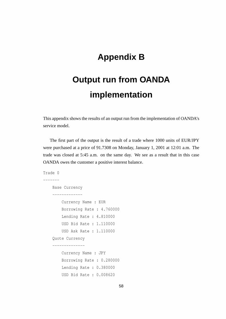
During a run of the implementation with some sample data, information was sent to

the console as output. The output of the program can be seen in Appendix B. I would

like to elucidate on some of the important parts of the implementation, as mentioned

in the program steps above, alongside some important associated issues.

Read currency and trades data In this step, the program reads two kinds of data,

currency data and trades data. Currency data is essentially the currency symbol

and required parameters during computation for the different currencies being

used. It follows the format below:

SYMBOL,BOR,LEN,BID,ASK

where SYMBOL is the currency code, BOR is the borrowing interest rate, LEN

is the lending interest rate, BID is the Bid US$ exchange rate and ASK is the

Ask US$ exchange rate. Each currency is on its own line, and an example is as

such:

EUR,1.90,2.30,1.1141,1.1143

Once a database of currency information is created in the program via the input

of the currency data, the program receives information about the specific trader’s

transactions, or his open trades in a service such as OANDA’s FXTrade.

BASE,QUOTE,TRANS,PRICE,UNITS,START,END

where BASE is the base currency, QUOTE is the quoted currency, TRANS is

the type of transaction, which is either BUY or SELL, UNITS is the number of

units traded in, START is the starting time and date of the trade, and END is the


ending time and date of the trade. START and END itself are decomposed into

the day, month, year, hour and minute units (can be decomposed into seconds if

required). An example format is as such:

EUR,JPY,BUY,91.7308,1000,5,7,2003,5,25,6,7,2003,5,15

An important point to note in this prototype is that data is being pre-read into

the program. However, the ultimate aim is to have this program connected to a

live (or historical) stream of data from a source such as one provided by Olsen

Data (Switzerland). This will enable the program to continuously read live data

and update its database so that all computations are based on current data. Thus

this input of data will cease to be a step in the execution of the program, and will

become a background process. Refer to Figure 3.1 for a visual view of this.

Calculate interest obtained and chargedThese steps in the program compute the

interest obtained by the trader from OANDA according to the formula shown

in Equation 4.1. When computing interest obtained by the trader, if it is a sale

transaction, then the number of units will be multiplied by the price to get the

real number of units in terms of the base currency. Similarly, when computing

interest charged to the trader, if it is a purchase transaction, then the number of

units will also be multiplied by the price.

Time computation For computation related to time in steps such as calculating dura-

tions of the trade, I have used much of the Standard Library (STDLIB) provided

by ANSI-C, and written code on top of it. Here, there is an implicit assumption

that the underlying code is free from errors, as well as the fact that it is accurate

in its computations. Even a slight loss of accuracy in computations related to

time can make an noticeable impact on the values calculated and care should be

taken in a real-world situation that the temporal computations are accurate.

4.2 The Greeks

Options are a very common derivative security traded today. However trading in op-

tions is not far from risky. Therefore traders use techniques to break down the risk in

a position that is easily understandable, and thus can be hedged. An important set of


analysis tools used is calledThe Greeks.

4.2.1 Volatility Background

The Greeks are the sensitivity of the option prices with respect to certain parameters

governing them. They are values the traders can look at and decide on an investment

strategy. This is because when people on the market trade options, they are essentially

tradingvolatility. When a trader purchases an option, he does so because he believes

that the market is volatile enough that he can trade/expose the option and earn a greater

profit than the amount he pays for the premium on the option. Similarly, when a trader

sells an option, it is because he feels that the premium that he earns on the sale is

greater than the profit he can make by trading the option on the market, because of its

lower volatility. Volatility is defined as the amount of variability in the returns of a

particular asset [Taleb, 1996]. There are essentially 2 types of volatility.

4.2.1.1 Historic volatility

Historic volatility is a measure of how much the market (in this case, the spot price)

moves over a specified time period. It is usually calculated as the standard deviation of

change in the price of the underlying asset over a period.

4.2.1.2 Implied volatility

Implied volatility (IV) is the market’s perception of the volatility of the underlying

security. Essentially, instead of estimating a volatility parameter to enter into an option

pricing model, such as the Black-Scholes pricing model (Section 5.1) and getting back

an option price, one can reverse the equation using current option prices in the market.

This results in the pricing model to output what is the calculated or implied volatility

of an option based on the current market price of the option.

4.2.2 The different Greeks

4.2.2.1 Delta

The Delta is the sensitivity of the option price to the change in the underlying asset

price. It is expressed as:

∆ =∆F∆U

(4.2)


where F is the derivative F(U,t) and U is the underlying asset.

4.2.2.2 Gamma

The Gamma is the sensitivity of the Delta to the change in the underlying asset price.

It is expressed as:

Γ =∆2F∆U2 (4.3)

where F is the derivative F(U,t) and U is the underlying asset.

4.2.2.3 Vega

The Vega is the sensitivity of the option price to the change in implied volatility (Sec-

tion 4.2.1.2). The simple Vega is expressed as:

Vega=∂F∂U

(4.4)

where F is the derivative F(U,t) and U is the underlying asset. Note: since there is no

Greek symbol for the Vega, sometimes Tau (τ) is used in place of it.

4.2.2.4 The other Greeks

There are a few other Greeks which serve as useful analytical tools, the more important

of which are:

Theta The Theta is the expected change in the option price with the passage of time,

assuming risk-neutral growth in the asset.

Rho The Rho is the sensitivity of the option price to interest rates, or to dividend

payout.

4.2.3 The Delta

The Delta is the first mathematical derivative of an option with respect to the underly-

ing asset. It is expressed as a percentage of the sensitivity of the underlying asset, or it

could also be expressed as the actual value of that percentage. The original definition

of the delta is:

Delta=∂F∂U

(4.5)

where F is the derivative F(U,t) and U is the underlying derivative. However, it is not

possible in the real world to gauge such values from an infinitely small change in the


price, and thus the definition of the delta is modified to be as in Equation 4.2. The

Delta could be further modified for accuracy also, e.g. to represent the up-movements

and the down-movements of the price better.

The Delta however is not restricted to options only. It can be as useful a tool for linear

derivatives (Section 2.1.2.1). Thus it is equally applicable to futures and forwards,

which is what this experiment deals with, specifically with a foreign currency forward.

The algorithms involved with computing the delta of a linear derivative use different

parameters, however.

4.2.3.1 Foreign Currency Forwards

The basic formula for computing the forward price for a foreign currency forward is

F = e(r−r f )tS (4.6)

The derivative security does not however immediately deliver profits or losses. There

is a waiting period till the settlement date. Since the profit turns into cash at the end

of the one-year forward, the profit/loss needs to be discounted back to cash using the

standard technique for a non-interest bearing asset. Thus usingSas the spot price,r as

the domestic interest rate,rf as the foreign interest rate, andt as the time to expiration,

we get

P/L o f F = e−rt e(r−r f )t∆S (4.7)

= e−r f t ∆S

Taking the derivative of that, to compute the Delta, we get

Delta= e−r f t (4.8)

4.2.4 Implementation

The aim of this experiment has been to set up the infrastructure around the computation

of Equation 4.8. This experiment was designed to take advantage of both the embedded

computation architecture as well as the reconfigurable logic architecture, i.e. the ARM

processor as well as the FPGA. This shows a prototype of how the embedded processor

could be used to control the processing, and guide the FPGA towards the raw data

processing.


4.2.4.1 The embedded component

This portion of the prototype is designed to be the link between real-time or non real-

time data sources and the FPGA, and thus prepares the data for quick computation on

the FPGA. The program executes the following steps:

Read Currency Data This program builds on the program written for computing in-

terest via OANDA’s financial model (Section 4.1 )and thus its input of currency

data is in the same form. It reads in data regarding specific currencies and pre-

pares its database for processing on trades. For the details of how the data is read

in, and its format, please refer to Section 4.1.4.

Read Trades Data As the focus on computation in this experiment is different from

the experiment mentioned above, its requirements of reading in data relating

to trades is also different. The program essentially needs the currencies being

traded and the expiry date and time of the forward contract. The format for the

data being read in is

BASE,QUOTE,EXPIRY

where BASE is the symbol of the base currency, QUOTE is the symbol of the

quoted currency, and EXPIRY is the time of the expiry of the forward contract.

EXPIRY is decomposed into the date, the month, the year, the hour and the

minute. It is also possible to modify the program to compute down to the seconds

although it has not been implemented currently. As in the financial markets, the

starting time is assumed to be now, i.e the forward is already active. And example

format is

CHF,JPY,13,7,2003,0,0

Output data for further computation In this step of the execution, the program re-

trieves the borrowing interest rate for the base currency, and the lending interest

rate for the fixed currency. It also computes the total time remaining for the ex-

piry of the forward, and outputs all of this data to a file for computation by the

FPGA. The format of output is


BASE/QUOTE

LEND

BOR

TIME

where BASE is the symbol of base currency, QUOTE is the symbol of the quoted

currency, LEND is the lending interest rate of the base currency, BOR is the

borrowing interest rate of the quote currency, and TIME is the number of seconds

left for expiry of the forward contract.

4.2.4.2 The reconfigurable logic component

For the next phase of computation in this prototype, VHDL has been used as a develop-

ment language for logic design. Other options were to go for a language like Verilog,

or to have a schematic design input. VHDL was chosen because of the short learning

curve and quick turnaround time in developing a prototype. For more details on this

selection, please refer to Section 3.2.2.

The Delta Entity In the program, an entity in VHDL has been described, calleddelta.

The ports in the entity are:

expiry This is an input port of type real. It is used for receiving the signal

containing the number of seconds till expiry of the forward contract.

rate 1 This is an input port of type real. It is used for receiving the signal

containing the lending interest rate of the base currency.

rate 2 This is an input port of type real. It is used for receiving the signal

containing the borrowing interest rate of the quote currency.

delta This is an output port of type real. It is used for sending the signal con-

taining the computed delta for the forward contract.

The behavioural description of the thedelta entity does the computation spec-

ified in Equation 4.8 and sends the output to the delta port in the entity. Since

the interest rates used are in percentage points, on a yearly basis, the number of

seconds also has to be taken on a yearly basis. Thus a constant has been defined

in the behavioural description of the entity which is the number of seconds in a


year, i.e. 31,536,000. The number of seconds till expiry is divided by this con-

stant. From a practical point of view, it may be required to change this constant,

if one were to assume the number of trading days in a year (∼ 250), rather than

the total number of days.

The Testbench A VHDL testbench has also been created, which is known asdelta tb.

Recall that the input data to this prototype comes from the embedded computa-

tion phase of the program. This testbench reads and interprets the data from

that output and sends the data across the signals to the delta entity. Given the

computation that is being performed currently, the lending rate of the base cur-

rency is not required to be implemented in the program. However, it has been

included in the data transfer and the model of the port for future use, i.e. it

should be relatively simpler to change the computation being performed without

adding another data element to the system. Also, the data is being read from

a file by the testbench. From a performance point of view, this does cause a

slight slowdown in the execution of the program, as disk I/O is usually slower.

The performance could be enhanced by embedding sample data for the proto-

type directly inside the testbench code. However, in this case such slowdowns

in performance are not relevant, as the ultimate aim is to put programs such as

these onto a processor-FPGA combination, and any bottlenecks will shift else-

where in the system. However, the core of of the computation engine will give

the performance desired by this experiment.

Chapter 5

Option Pricing

Option pricing has been a matter of significant research and study since several years,

and a sizeable proportion of research into the mathematical modelling of financial

markets has gone into this field. The problem basically entails computing a fair value

for the price of an option, although it is also used to calculate values such as implied

volatility (IV). As early as 1900, the French mathematician Louis Bachelier wrote

about pricing options using geometric Brownian motion. He used these techniques

to model options on French government bonds. However, the biggest breakthrough

came in 1973, when Fischer Black and Myron Scholes published their landmark paper

describing the Black-Scholes option pricing theory. There had also been earlier work

in the field by Samuelson, and later on improvements in option pricing theory by John

Hull and Alan White.

5.1 Black-Scholes Option Pricing

The Black-Scholes option pricing theory is the most commonly used model for pricing

of options by academics and traders alike. It makes several assumptions, some of

which seem unrealistic, and have been addressed by further research into newer, more

accurate models. Nevertheless, the Black-Scholes model of option pricing continues

to be the among the most used tools to dynamically hedge an option in the market.

Some of the important assumptions of the model are:

• The price of the underlying asset follows a geometric Brownian motion, and has

constant volatility. The fact that it has constant volatility is known not to be true

and has been addressed by Hull-White in [Hull and White, 1987]. Due to this,

the model generally overprices models, as most trading happens with the strike

35

Chapter 5. Option Pricing 36

price being within 10% of the underlying asset price, and the model is shown to

have overpriced options that are close to being at the money.

• There are no transaction fees.

• The risk-free interest rate does not change with respect to time.

• Arbitrage in the market is not risk-free.

The model defines a partial differential equation, as in Equation 5.1.

∂V∂t

+12

σ2S2∂2V∂S2 + rS

∂V∂S− rV = 0 (5.1)

The above is a second order differential equation, and is general in nature. Different

boundary conditions can be applied to make it price any option. Black and Scholes

specifically applied boundary conditions to this differential equation for a European

call option, and this resulted in the following formula, called the Black-Scholes option

pricing formula as in Equation 5.2, Equation 5.3 and Equation 5.4.

PCall(S,X,σ,R,T) = Sφ(d1)−Xe−RTφ(d2) (5.2)

d1 =loge( S

X )+(R+ σ2

2 )Tσt

(5.3)

d2 = d1−σ√

T (5.4)

where

PCall is the price of the European option call

S is the current price of the underlying asset

X is the strike price

σ is the implied volatility

R is the risk-free interest rate, compounded continuously

T is the time till expiration, in years

φ is the standard normal cumulative distribution function (Section 5.2)

The concept of put-call parity in financial mathematics allows us to have a relation-

ship between calls and puts in options, if they have a similar strike price and expire at

the same time. This allows one to derive a formula for a European style put option as

in Equation 5.5.


PPut = PCall +Xe−RT−S (5.5)

where all the variables are as defined above.

5.2 Standard Normal Distribution

The standard normal distribution is an important part of option pricing with the Black-

Scholes model. Financial variables often exhibit scales that fit the normal distribution

quite well, such as interest rates and exchange rates. The normal distribution is essen-

tially another name for a Gaussian distribution. The variables affecting the distribution

are themeanµ and thestandard deviationσ2. The probability density graph looks like

a Gaussian curve (Figure 5.1) and theprobability density functionis

P(x)dx=1

σ√

2πe−

(x−µ)2

2σ2 dx (5.6)

If we take the meanµ = 0 and the standard deviationσ2 = 1, we get the standard

normal distribution, whose probability function is

P(x) =1√2π

e−x22 (5.7)

For the standard normal distribution function, the distribution function looks Sig-

moid (Figure 5.2 )and is given by

D(x) =er f( x√

2)+1

2(5.8)

5.2.1 The Erf function

The erf function is the error function which occurs when the standard normal distribu-

tion function is integrated. It is defined as

er f(x) =2√π

∫ x

0e−t2

dt (5.9)

The complimentary function erfc is defined as

er f c(x) =2√π

∫ ∞

xe−t2

dt (5.10)

er f c(x) = 1−er f(x) (5.11)


-0.05

0

0.05

0.1

0.15

0.2

0.25

0.3

0.35

0.4

0.45

-3 -2 -1 0 1 2 3

X

P(X

)

Figure 5.1: PDF of the Standard Normal Distribution

-0.2

0

0.2

0.4

0.6

0.8

1

1.2

-3 -2 -1 0 1 2 3

X

D(X

)

Figure 5.2: CDF of the Standard Normal Distribution


5.3 Reference computation

In [Benninga and Wiener, 1997b], the objective of the authors is to show numerically

that using the binomial option pricing formula shown in [Benninga and Wiener, 1997a],

the price converges to the price as as computed using the Black-Scholes option pricing

formula. This is shown to be true for European style options and some American style

options. In doing so, they provide an implementation for the Black-Scholes option

pricing formula, which I have used as a reference point for computation and perfor-

mance testing. This implementation is on the Mathematica environment, and is also

available in an electronic form along with the paper. An extract of the relevant parts of

the code from this paper is shown in Appendix A.

5.3.1 Reference standard normal distribution

In [Benninga and Wiener, 1997b], the authors have noted that it is possible to compute

the values of the standard normal distributions in many different ways, and they show

four different methods of computation. They are

Integration In this approach, the standard normal distribution as shown in Equation

5.7 is integrated as below. ∫ x

−∞

ez2/2√

2π(5.12)

Numerical approximation In the second approach, a numerical approximation of

Equation 5.12 is computed.

Distribution Function Here, the distribution function of the standard normal distri-

bution as shown in Equation 5.8 is computed.

Normal Distribution In the fourth approach, the built-in package of Mathematica for

sampling a normal distribution is used, and given values of 0 and 1 for the mean

µ and the standard deviationσ2 to get a sample value.

The reason for having so many approaches is to show how computationally intensive

a specific approach can get. In the paper, the authors show the results of timing the

sampling of 100 values from each approach, of which the third approach is shown to

be the fastest, and just under 2000 times faster than the first approach. Since the third

approach is not only the fastest, but also the most feasible to implement on reconfig-

urable logic, that is my chosen approach for both implementation and performance

measurement.


5.4 Implementation

The computations involved in the Black-Scholes algorithm are rather complex and very

intensive, and thus implementations were done on both an FPGA as well as an ARM

processor independent of each other.

5.4.1 FPGA Implementation

After due consideration, and taking into account the advantages of VHDL over Verilog

described in Section 3.2.2, VHDL was used for describing the logic in the component,

and it was targeted towards a Xilinx Virtex II Pro FPGA.

5.4.1.1 Entity and Testbench

The VHDL logic defines a basic VHDL entity calledbsPrice. This entity receives

input values, does the required computations via the Computations package (Section

5.4.1.2), and returns the results via its output ports. The ports defined in the entity are

directly derived from Equation 5.2 and Equation 5.5 and are as below

S This is an input port of type real. It represents the current price of the underlying

asset of the option.

X This is an input port of type real. It represents the current strike price of the deriva-

tive security, the option.

Sigma This is an input port of type real. It represents the implied volatility (Section

4.2.1.2) of the option.

T This is an input port of type real. It represents the time till the expiration of the

option, in years.

Rf This is an input port of type real. It represents the current risk-free interest rate.

isACall This is an input port of type integer. It is essentially a control port, that spec-

ifies whether the price to be computed is for a put option or a call option. Since

the variables required for computation are the same, this port suffices as the only

control port.

Price This is an output port of type real. It is used to output the price of the call or the

put, after computation.


The behavioural description of the bsPrice entity looks at the control port value and

sends data on the output port accordingly. If the isACall has a value of ”1”, then the

call pricing function in the Computations package is called, or if the signal has a value

of ”0”, the put pricing function in the computation is called. For a third control value of

”2”, the FPGA disables the processing of the algorithm, and does not send any signal

on the output port.

The testbench associated with the above entity is bsPriceTB. The input values have

been hardcoded into the testbench, but they have also been tested to be read from

external data sources, like a virtual console or a file.

5.4.1.2 Associated Computations package

All the computations as described in the set of equations described in Section 5.1

and Section 5.2 have been implemented within a package external to the entity, in an

attempt to modularise the implementation, and make it more extensible. The functions

thus created in the package are

bsCall This function is a top-level function for computing the price of a call option. It

implements Equation 5.2.

bsPut This function is a top-level function for computing the price of a put option. It

implements Equation 5.5.

d1 This function computes thed1 function as described in Equation 5.3.

d2 This function computes thed2 function as described in Equation 5.4.

snormal This function is a top-level function for sampling a value from the standard

normal distribution using the computation described in Equation 5.8.

erf The erf function is used for obtaining a value from the standard normal distribu-

tion and is defined as in Equation 5.9. However, its implementation is a little

different in this context. Since its computation involves approximating an inte-

gral, it is not feasible to implement an architecture for calculus on reconfigurable

logic within the scope of this project. Also, the purpose of implementing this on

an FPGA is to increase the speed of processing, thus implementing an infras-

tructure for calculus processing would be counter-productive. Thus I used a

numerical approximation for the function, which I adapted from a version used

in the Radiance project [RadianceOnline, 2003]. Also, a full implementation of


the function has not been done, but only the part required to handle the specific

input values that can be expected in the sample data. It is a trivial task to com-

plete the function to handle all possible data values, but it is not required in this

scenario.

5.4.2 ARM implementation

The ARM implementation of the reference computation was done in ANSI-C, and tar-

geted towards a ARM 7 processor. The basic functions implemented in the program are

the same as described in the Computations package in FPGA implementation (Section

5.4.1.2).

5.4.3 Results

The reference computation in this experiment has been implemented in Mathematica.

The intent at the start of the experiment was to implement equivalent processes on

independent components of the soft-hardware platform (on reconfigurable logic as well

on an ARM processor) and have a direct comparison of the performance. As a result,

the implemented designs are behaviourally similar to the reference computation, as

well as having utilised the same or equivalent techniques. This is evident from the

following points.

Black-Scholes formula To compute the actual pricing for the call option and the put

option, the same formula has been used, as defined in Equation 5.2, 5.3, 5.4 and

5.5. No optimisations were made to affect performance in any way, although

in an implementation targeted for regular use, rather than comparison, the algo-

rithms should be tweaked in all possible ways.

Standard Normal Distribution implementation As with the Black-Scholes pricing

formula, the same method of sampling a value from a Standard Normal Dis-

tribution has been used, as defined in Equation 5.8. It may be recalled from

Section 5.3.1, that the fastest technique was chosen and used by the reference

computation as well as both these implementation.

Erf function Recall from Section 5.4.1.2 that it is infeasible for the scope of this

project to implement a calculus computation infrastructure on the FPGA. Thus, a


numerical approximation has been implemented instead. However, in the refer-

ence computation too, the implementation uses Mathematica’s built-in Erf func-

tion, and may be assumed to have suitable optimisations or approximations in-

stead. For the implementation on the ARM processor, the libraries which accom-

pany the development and simulation environment provided an implementation

of the Erf function, which was used. It is assumed that this function also uses a

numerical approximation.

Input data For the purposes of the intended evaluation, the same values of input data

were given to the three implementations, and are the same as used in the refer-

ence paper, as in [Benninga and Wiener, 1997b]

To verify that the implementations on the different platforms was similar and correct,

an initial test was conducted. The output from runs on the Mathematica platform and

the embedded ARM platform were captured, and plotted. Similar values of input data

as shown in Table 5.1 were given to the implementations to compute the Black-Scholes

price for a call option and a put option, and the time to expiry (in years) was varied from

0 to 1. As we can see in Figure 5.3 for the Mathematica implementation and Figure

5.4 for the ARM Processor implementation, the results of both the implementations

are the same. It was infeasible to run a similar test on the FPGA implementation, due

to the granularity of the test. However, randomly chosen values from the set of input

data for this test were used in the FPGA implementation and the output was verified to

be the same.

To test performance however, different input values should be preferably used for the

put and call pricing functions, although the data would be common across the three

different platforms. The input data for these functions used in the performance test is

as shown in Table 5.2. For a description the variables in the input data, please refer to

Section 5.4.

For the Mathematica based implementation, it was quite straightforward to analyse

the time taken for computation. A loop based test for 10000 iterations of execution of

both call and put pricing algorithms was conducted. Each iteration consisted of one

call to a call pricing function,bsCall and one call to a put pricing function,bsPrice.

This test yielded an approximate computation time of 15.625µs for each iteration. The

test was conducted on Mathematica 5.0 running on an Intel Pentium 4 processor, with

a clock speed of 2.53 GHz.


Figure 5.3: Mathematica : Black-Scholes verification

0

2

4

6

8

10

12

14

0 0.2 0.4 0.6 0.8 1

Expiry in Years

Op

tio

n P

rice

Call Option

Put Option

Figure 5.4: ARM Processor : Black-Scholes verification


Variable bsCall bsPrice

S 50.0 50.0

X 45.0 45.0

Sigma√

0.2√

0.2

T 0 to 1 0 to 1

Rf 0.06 0.06

Table 5.1: Input data for verification test

Variable bsCall bsPrice

S 50.0 45.0

X 45.0 45.0

Sigma√

0.2 0.3

T 0.25 1.0

Rf 0.06 0.08

Table 5.2: Input data for performance test

On the ARM processor, performance testing was done on a simulated ARM7TDMI

processor. In the implementation, themain function calls both the bsCall and bsPut

functions in one iteration, and to reduce the effect of bias due to the program’s startup

and shutdown overhead, the iteration count was set at 10000. To estimate execution

time, the formula as shown in Equation 5.13 is used.

Execution Time=Number o f CPU Cycles

Speed o f Processor(5.13)

Simulation of execution of the program on the ARM processor showed that there were

a total of 345,582,880 CPU cycles consumed. I simulated the execution on an ARM

processor capable of speeds of 200Mhz, i.e. capable of doing2×108 calculations per

second. Thus plugging these values into Equation 5.13, we get the execution time as

1.7279144 seconds. Recall that this is the execution time for 10000 iteration, and this

gives an approximate time of execution for each iteration to be 170µs. This computa-

tion was floating point based, and the target ARM processor in the simulation did not

have a floating-point coprocessor installed. Thus, all floating point computation was

simulated within the processor itself, as was revealed by the results of profiling the

execution on the processor. With a floating-point coprocessor installed, it is estimated

that this number will reduce significantly, as the wrapper calls for the floating point


simulation will be removed, thereby lowering the CPU cycle count. Conservative es-

timates, taking into account the profiling report, show that the execution time could

drop by approximately 1% to 2%, and thus may be disregarded in the context of this

experiment due to the minor changes shown.

For the FPGA based implementation however, the design could not be synthesised due

to it being a purely floating-point computation. For further details, please refer Section

6.2.1. However, some modifications were made to the design to make it integer based.

These modifications render the output of the program incorrect, but the emphasis of the

changes made was to have a relatively similar number of units of computation. With

these modifications, it was possible to synthesise the logic, and derive performance

measures. A timing report yielded that this design has a minimum input arrival time

before the clock of 30.091 ns for each iteration of the pricing of a call option and a

put option, as in the test for the reference computation. Of this time, approximately

25.273 ns (84%) was logic time (combined latency of the blocks), and 4.818 ns (16%)

was routing time. Also, the timing report shows that the design had a maximum output

required time after the clock of 7.189 ns. This consisted of 6.781 ns logic time (94.3%)

and 0.408 ns of routing time (5.7%). However, before any conclusion are drawn on the

basis of these results, the following points need to be strongly emphasised.

• This logic had been modified to perform approximately similar number of com-

putations. The actual numbers will most probably not match, but should be in

the close vicinity of each other.

• These results are for integer based calculations, not real numbers as the original

design is.

• It was not possible to modify the computation of the Erf function in the design,

and thus the functionality was reduced to simply being an additional function

call in the RTL, and will be represented by a small block in the resultant FPGA

architecture. However, equivalent computations and execution profiling done on

an embedded ARM processor yielded that the Erf function contributes for less

than 4% of the computation in an iteration. This results in the impact of this

significant modification to be lessened.

Thus, rough approximations can be made to assume that the actual design can have

25% to 30% more total latency than this modified design. These approximations are

justified only via a visual inspection of the changes, however. Thus, one can expect


a total latency time for the actual design to be less than 50 ns. Another point to note

is that this design hasnot been pipelined, and is a straightforward, almost serially

executing design. Pipelining of this design to provide parallel execution, this latency

time can be greatly reduced. One of the primary motivations behind considering a

soft-hardware architecture as compared to a pure software environment has been the

natural parallelism that is available (Section 2.2.2.1). Thus it is natural to assume

that this FPGA design should be pipelined to fully extract the desired and expected

performance. Performing a mental analysis of the functioning of the Black-Scholes

option pricing formula, conservative estimates can be made that the pipelined version

should reduce the latency time by at least 50%, if not more, giving an approximate

total latency time of approximately 25 ns.

Chapter 6

Analysis and Conclusions

In this chapter, I shall provide an analysis of the results of the third experiment, and

then look at issues encountered during the design and implementation phases of the

experiments. Then I shall state the conclusions drawn from these experiments and talk

about future work to extend this project.

6.1 Evaluation of results

Since the first two experiments, on interest rate derivatives do not have a reference point

for performance, any performance measures from them would not have much bearing

and impact on the conclusions. What is important from those two experiments is the

actual design and implementation phase which exposed problems, and gave valuable

inputs to the feasibility aspects of this project, as well as to the perceived advantages.

For the third experiment however, there are also some interesting results that should be

considered.

6.1.1 Option Pricing experiment results

Based on the results shown in Section 5.4.3, a summary of the time taken to execute

one interation each of a call option pricing and put option pricing is as in Table 6.1.

It may be noted that the reference computation on Mathematica and the imple-

mentation simulated on an ARM processor have very similar number of computational

units, due to the similarities in performance. The processor that Mathematica ran on

was approximately 12.95 the speed of the ARM processor, as may be recalled from

Section 5.4.3. Consequently the implementation done on the ARM processor took ap-

48

Chapter 6. Analysis and Conclusions 49

Experiment platform Time per iteration Accuracy

Mathematica - Reference 15.625µs Very High

Simulated ARM processor 170µs High

Reconfigurable Logic 50 ns Medium-High

Table 6.1: Summary of results

proximately 10.9 times longer. The small difference in per MHz performance may be

attributed to the simplicity of the implementation on the ARM processor, as compared

to the overhead of Mathematica. Mathematica is a very large and complex package,

and due to its capabilities will probably have a significant amount of overhead. It must

be emphasised however, that Mathematica is a very respected software package for

efficient computation, and can in no way be considered unequal to the task. However,

the implementation on the FPGA was vastly more efficient than both of them. The

un-pipelined version took approximately 1% of the time to perform a similar computa-

tion, and the pipelined version should be at least twice as fast, as noted earlier on. This

shows a clear advantage of having raw processing done on the reconfigurable logic

platform. Also, the application could be suitably partitioned between the ARM pro-

cessor and the FPGA to extract maximum performance, given the known advantage

that ARM processors have in complex control routines over FPGAs. This will espe-

cially come in useful, as a possible commercial implementation of such an architecture

would be several time more complex, and would require careful control. It is expected

however, that the performance advantages seen in this smaller scale experiment will

manifest themselves in a bigger scale too.

6.2 Issues encountered

In all the experiments, as well as in the preliminary analysis stage, several obstacles

were seen in this approach. Most of them were overcome in a rather simplistic manner,

however there are some larger issues that still remain. These issues would need to be

tackled in a strong dedicated effort, but and can definitely be overcome. Some of the

important ones are discussed below.


6.2.1 Floating-Point computations

One of the major problems encountered during the course of this project is that em-

bedded systems and FPGAs are not naturally suited for floating point computation.

Embedded ARM processors usually come with a floating-point coprocessor, or have

soft floating-pointsupport, which allows them to emulate this capability with only a

small performance hit. The major problem however, comes when working with recon-

figurable logic. As with ASICs, FPGAs cannot directly handle any form of floating

bit-width in the computation. This is due to the very nature of hardware, that is pre-

configured to work with a specific set of signals, and cannot dynamically adapt to a

different combination set of a signal. This problem was encountered in two exper-

iments in this project, which were the implementations of the Delta and the Black-

Scholes Option pricing formula. In both cases, the design could not be synthesised

to get accurate performance results. The designs were not synthesisable because the

IEEE math library that was used for the floating point computations was designed for

simulation only. Also, when working with financial applications, almost all the compu-

tations involved are composed of real numbers, rather than integers. All the variables

used as parameters to the algorithms, such as interest rates, stock prices, expiry times

among others cannot be represented with the set of integers. However, this is not an

impediment of the form that invalidates this approach entirely. On investigation, sev-

eral solutions were found, although it was not feasible to employ any of them in this

project, due to resource constraints, both temporal and monetary. Some of the consid-

ered solutions include

Commercial floating point IP cores There are several commercial floating point IP

cores available, which can be integrated within the logic design during the design

capture phase. These products give floating point computational abilities com-

patible with the IEEE 754 standard, and usually provide very good performance

too. Some of the companies providing these IP cores are Transtech, Digital Core

Designs, Nallatech, ASICS, Altera and Digital Engineering. The only known

downside to these products is the cost, although it remains to be seen how well

they integrate with the different FPGAs in the market.

Public domain floating point libraries There are some synthesisable floating point

libraries available for free, but they usually do not support all floating-point op-

erations, and performance is suspect. It is not a viable option for a commercial

undertaking as yet, although there may be some libraries that would be suitable


for testing and verification purposes.

Fixed point computation Using fixed point computational techniques instead of float-

ing point is a very viable solution to this problem. This process does involve ad-

ditional effort though, as most development tools or libraries do not have direct

support for fixed point computation. For more details on fixed-point compu-

tation, please refer to Section 6.4.1. However, progress is being made in this

regard, with efforts for incorporating fixed-point design in embedded and recon-

figurable logic systems ([Menard et al., 2002]).

Integer based computation This is a last resort option, however quite achievable.

Basically, all real numbers in the application are converted to integers, by multi-

plying by a pre-decided number before being sent to the FPGA. After processing

is complete, these numbers are reconverted back to real numbers in floating point

storage. However, this technique is not always applicable, and may not work for

anything more than the simplest of cases.

6.2.2 Data acquisition

When working on financial algorithms, it is often hard to come by good sample data

for input. In most cases, the data is sold as a service by some company, and it is

expensive to get huge reams of data to work with during the design process. Smaller

amounts are more accessible, but that accordingly affects testing efforts. In this project,

Olsen Ltd. has been very generous in providing input data for testing the algorithms,

however, to get exactly the kind of data that is being used, often may turn out to be

expensive. Also, the data itself may need some massaging and modification to suit the

program, and there may be a requirement for the computation engine to perform this

modification itself. Of course, it would not be rational to embark on such a project

without being confident of availability of data during actual execution, however this is

an issue that mostly limits itself to the design and implementation phases.

6.2.3 Mathematical infrastructure for computation

The financial industry and markets are one of the major target areas of applied mathe-

matics. As a result, the models used in the computations in this sector are rather com-

plex, and usually delve deeper than within the confines of simple integer arithmetic.


This results in financial models that are very heavily dependent on calculus, probabil-

ity, statistics and other fields of mathematics. Thus, a mathematical infrastructure is

required for tasks such as the following.

• Integration

• Higher Order Derivation

• Random Number Generation

• Statistical and Stochastic Modelling

• Vector Calculus

• Trigonometric Functions

• Logarithmic Functions

The fundamental functions of these do appear in several software libraries, and the

advanced ones use specialised packages such as Mathematica and Matlab. However, if

the financial algorithms which use all these functions are to moved onto an FPGA, then

logic libraries need to be available to perform such functions, as currently there is only

very basic support for these applications of mathematics. A recommended approach

would be to develop such a computational infrastructure for FPGAs and embedded

processors first, and then the implementation of various different financial algorithms

would be much simpler.

6.3 Conclusions

It is apparent from the experiments conducted, and the research that went into their

design that implenting a programmable real-time trading architecture on a processor-

FPGA platform is a step in the right direction. The work has been a little harder than

expected, due to the relative lack of previous work into this specific field. It is mostly a

novel idea, and has yielded positive results. The specific observations can be summed

up by discussing the feasibility and the advantages of such an approach.

6.3.1 Feasibility of approach

As mentioned in Section 6.2, there have been a few problems in this project, some of

which remain unsolved, although possible solutions have been investigated. However,


those issues can be considered almost minor as compared to the general feasibility that

has been encountered in the project. All throughout the experiments, the primary ob-

servation has been that financial algorithms are quite suitable for implementation on

a processor-FPGA architecture. Although RTL languages like VHDL and Verilog are

powerful enough to express most algorithms with ease, there is additional help avail-

able from other quarters. Gradually, there has been an increase in the availability of

tools and techniques for programming hardware from a strongly software engineer-

ing style approach. As mentioned in Section 3.2.2, it is not possible to use high-level

languages such as C, C++ and Java, along with variants like SystemC and Handel-C

for use in such applications. Although for high performance, it is preferred to design

directly in RTL, using high-level languages has proved to be a worthwhile solution,

both for programming hardware as well as for writing programs for an embedded pro-

cessor. Financial algorithms are generally easy to express once an infrastructure for

mathematical computation, as mentioned in Section 6.2.3 is in place. It has also been

especially noted that financial computation algorithms are quite suitable for partition-

ing between an ARM processor and and an FPGA, as they are traditionally contain

control intensive segments as well as raw computational units.

6.3.2 Benefits of approach

Experimentally, it is seen through the analysis of the results of the experiment involving

implementation of the Black-Scholes option pricing formula in Section 6.1.1, that there

is a clear advantage in performing computations, especially financial computations on

an FPGA as compared to a general purpose or embedded processor. The control re-

lated segments of the application however, may be better suited for a processor than an

FPGA. Also, it is important to note that a simple, and more targeted implementation

of the experiment on the ARM processor performed slightly better than the implemen-

tation on the Mathematica platform on a general purpose desktop CPU. Although the

difference is slight, it highlights the need to shift away from a generic software envi-

ronment for financial computation packages.

However, performance is the not the only benefit perceived from a shift to this architec-

ture for financial trading. Ease of use contributes greatly to the strength of such a plat-

form. Traders in the financial markets use tools built on platforms such as Mathematica

to perform analysis and get the information they need. One such tool was looked at,

called UnRisk. It is a numerical engine that contains a numerical computation engine


implemented in C++, and connects to Mathematica for symbolic manipulation and vi-

sualisation. One of the primary and powerful front-ends for the tool is Mathematica

itself. UnRisk allows a trader to perform many derivative analysis tasks, including

sensitivity analysis. It allows a trader to build models of complex contracts and extract

various numerical and visual results from it. However, using Mathematica as a front

end for such work is slow, cumbersome and prone to error. Also, the average financial

trader would not be expected to be comfortable using programming techniques for data

analysis. This project recognises that as a problem, and aims to make such data analy-

sis easier for traders to use. Referring back to the architecture as envisioned in Figure

3.1, an interface could be provided to a user wherein he simply receives realtime anal-

ysed results from the data, while still being able to parameterise the computation. This

form of an architecture can specifically be viable when a processor-FPGA combination

is used for the Computation Engine, as the process of providing fluidity of analysed

data to the trader would require heavy computational power.

6.4 Future Work

One of the obvious extensions to this work could be work on the solutions to the issues

mentioned in Section 6.2. This would involve the possible creation of a fixed-point

library for computation as a very likely candidate, along with the development of an

infrastructure for mathematical computation, as required by the financial algorithms

dealing with derivative trading. Also, given the conclusions of this project, it seems

feasible to extend this work by working on the implementation of a more complex

algorithm in this field, such as the Hull-White model for option pricing, as shown in

[Hull and White, 1987].

6.4.1 Fixed-Point Computation

In this technique, the position of the decimal separating the integer and fraction por-

tions of the number is fixed, rather than floating. First, all the real numbers being input

into the logic are converted to a vector representation [Seidel, 2003], and a total width

size W is chosen, based on the level of precision required. For e.g., when working in

the radix 10, if W is set to 4, then 0.5 can be represented by0.510×10W/2 = 005010.

This vector format is then used for the required arithmetic operations such as addition

and subtraction as normal. For multiplication and division, there is a scaling problem


encountered, which can be overcome with a slight loss of precision. At any time, this

bit vector can be represented as a real number by converting it back again. For e.g.

005010÷10W/2 = 0.510.

6.4.2 Mathematical Infrastructure

As mentioned in Section 6.2.3, further work would be greatly helped by the devel-

opment of a library of mathematical functions. However, one should choose a base

architecture for computations on real numbers first. For example, if fixed-point com-

putation is decided as the most favourable approach to pursue, then the mathematical

library should use fixed-point data types for all computations.

6.4.3 Hull-White model

This model adds a complexity factor by assuming that the volatility of a derivative

security is stochastic in nature, and not fixed, as assumed in the Black-Scholes model

of option pricing. This model would be able to provide financial traders with even

greater accuracy in pricing, as compared to the Black-Scholes model, which has known

problems due to its assumptions (Section 5.1). This could lead to greater adoption of

the Hull-White model, which so far has been limited given its complexity. Building

on a base such as the one proposed in this project, and taking advantage of the soft-

hardware architecture to provide high performance would be highly instrumental in

abstracting the complexity from the market operators.

Appendix A

Reference Black-Scholes

implementation

This appendix contains an extract of the relevant portions of the reference implemen-

tation of the Black-Scholes option pricing formula used in the third experiment.

The first part of the extract describes the definition of the different functions for

sampling a value from a standard normal distribution.

snormal1[x_]:= Integrate[Exp[-z2/2]/Sqrt[2*Pi],

{z,-Infinity,x}]//N

snormal2[x_]:=

NIntegrate[Exp[-z2/2]/Sqrt[2*Pi], {z,-Infinity,x}];

snormal3[x_]:= Erf[x/Sqrt[2]]/2+0.5; In[2]:=

Needs["Statistics‘Master‘"] ndist=NormalDistribution[0,1]; In[3]:=

snormal4[x_]:=CDF[ndist,x]//N;

In this second portion of the code extract, the functions representing the Black-

Scholes option pricing formula are defined.

In[5]:= Clear[snormal, d1, d2, bsCall, bsPut] snormal=snormal3;

d1[s_, x_, sigma_, T_, r_]:= (Log[s/x]+(r+sigma2/2)*T)/

(sigma*Sqrt[T]) d2[s_, x_, sigma_, T_, r_]:= d1[s, x, sigma, T,

r]-sigma*Sqrt[T] bsCall[s_, x_, sigma_, T_, r_]:=

s*snormal[d1[s,x,sigma,T,r]]-x*

Exp[-r*T]*snormal[d2[s,x,sigma,T,r]] bsPut[s_,x_,sigma_,T_,r_]:=

bsCall[s,x,sigma,T,r]+x*Exp[-r*T]-s

56

Appendix A. Reference Black-Scholes implementation 57

In this final portion, the functions are called for one iteration of pricing a put option

and a call option. The results are also shown.

bsCall[50, 45, Sqrt[0.2], 0.25, 0.06]

bsPut[45, 45, 0.3, 1, 0.08]

7.62426

3.61033

Appendix B

Output run from OANDA

implementation

This appendix shows the results of an output run from the implementation of OANDA’s

service model.

The first part of the output is the result of a trade where 1000 units of EUR/JPY

were purchased at a price of 91.7308 on Monday, January 1, 2001 at 12:01 a.m. The

trade was closed at 5:45 a.m. on the same day. We see as a result that in this case

OANDA owes the customer a positive interest balance.

Trade 0

-------

Base Currency

-------------

Currency Name : EUR

Borrowing Rate : 4.760000

Lending Rate : 4.810000

USD Bid Rate : 1.110000

USD Ask Rate : 1.110000

Quote Currency

--------------

Currency Name : JPY




58

Appendix B. Output run from OANDA implementation 59


Transaction : BUY

Price : 91.730800

Units : 1000

Duration : From 1/1/2001, 00:01 to 1/1/2001, 05:45

Difference : 0.034557 - 0.001947 = 0.032610

In the second part of the output run, we examine a trade where 2000 units of

GBP/CHF were sold at the price of 2.5822 on Monday, January 1, 2001 at 4:00 a.m.

This trade was closed at 5:45 a.m. the same day.

Trade 1

-------

Base Currency

-------------

Currency Name : CHF





Quote Currency

--------------

Currency Name : GBP





Transaction : SELL

Price : 2.582200

Units : 2000

Duration : From 1/1/2001, 04:00 to 1/1/2001, 05:45

Difference : 0.023586 - 0.038090 = -0.014504

Bibliography

[Ashenden, 1990] Ashenden, P. (1990). The VHDL cookbook. On-

line copy viewed July 2003 : http://tech-www.informatik.uni-

hamburg.de/vhdl/doc/cookbook/VHDL-Cookbook.pdf.

[Benninga and Wiener, 1997a] Benninga, S. and Wiener, Z. (1997a). The binomial

option pricing model.Mathematica in Education and Research, 6(3):27–34.

[Benninga and Wiener, 1997b] Benninga, S. and Wiener, Z. (1997b). Binomial option

pricing, the Black-Scholes option pricing formula, and exotic options.Mathematica

in Education and Research, 6(4):11–14.

[Bingham and Keisel, 1998] Bingham, N. H. and Keisel, R. (1998).Risk-Neutral Val-

uation : Pricing and Hedging of Financial Derivatives. Springer Verlag.

[Bombay Stock Exchange, 2003] Bombay Stock Exchange, I. (Viewed : May 2003).

Introduction to derivatives. http://www.bseindia.com/faqs/intro.asp.

[Brown and Rose, 1996] Brown, S. and Rose, J. (1996). Architecture of FPGAs and

CPLDs: A tutorial.IEEE Design and Test of Computers, 13(2).

[Dacorogna et al., 2001] Dacorogna, M. M., Gencay, R., Muller, U. A., Olsen, R. B.,

and Pictet, O. V. (2001).An Introduction to High-Frequency Finance. Academic

Press.

[DerivativesRUs, 2003] DerivativesRUs (Viewed : June,

2003). Forward contracts and futures contracts,

http://www.ivey.uwo.ca/faculty/ssapp/teaching/derivatives/dru/v1n15.htm.Deriva-

tives R Us, 1995, 1(15).

[Hull and White, 1987] Hull, J. and White, A. (1987). The pricing of options on assets

with stochastic volatilities.Journal of Finance, 42(2).

60

Bibliography 61

[Hull and White, 1990] Hull, J. and White, A. (1990). Pricing interest rate derivative

securities.The Review of Financial Studies, 3.

[Humphrey, 1995] Humphrey, W. S. (1995).A Discipline for Software Engineering.

Addison-Wesley.

[Hwu, 2003] Hwu, W.-M. (Viewed: July, 2003). Computing with FPGAs and recon-

figurable logic. http://courses.ece.uiuc.edu/ece311/lectures/lecture18.pdf.

[Kozlowski, 2002] Kozlowski, A. (2002). Derivative pricing with mathematica. In

6th World Multiconference on Systemics, Cybernetics, and Informatics. Toyama In-

ternational University, Japan.

[Menard et al., 2002] Menard, D., Chillet, D., Charot, F., and Sentieys, O. (2002).

Automatic floating-point to fixed-point conversion for DSP code generation.CASES

2002, pages 8–11.

[Moore and Luk, 1991] Moore, W. R. and Luk, W., editors (1991).FPGAs. Abing-

done EE&CS Books. Edited from the Oxford 1991 International Workshop on Field

Programmable Logic and Applications.

[Moore and Luk, 1993] Moore, W. R. and Luk, W., editors (1993).More FPGAs.

Abingdone EE&CS Books. Edited from the Oxford 1993 International Workshop

on Field Programmable Logic and Applications.

[OANDA, 2003a] OANDA (Viewed : June 2003a). Effects of continuous interest rate

payment. http://fxtrade.oanda.com/fxtrade/interestpayment.shtml.

[OANDA, 2003b] OANDA (Viewed : June 2003b). Oanda interest rate calculation.

http://fxtrade.oanda.com/fxtrade/interestcalculation.shtml.

[Paskov and Traub, 1995] Paskov, S. and Traub, J. (1995). Faster valuation of finan-

cial derivatives.The Journal of Portfolio Management, 22(1):113–120.

[RadianceOnline, 2003] RadianceOnline (Viewed : July 2003). www.radiance-

online.org.

[Seidel, 2003] Seidel, S. (Viewed : August 2003). Fixed point numerical representa-

tion. http://www.aftersleeves.org/projects/fixed.html.

Bibliography 62

[Smith, 2003] Smith, D. J. (Viewed : July 2003). Vhdl & verilog com-

pared & contrasted plus modeled example written in vhdl, verilog and c.

http://www.esperan.com/vhdlvlogcompared.pdf.

[Soudan, 2000] Soudan, B. (2000). Using FPGAs with ARM processors.Xilinx,

(WP123).

[Srinivasan, 2002] Srinivasan, A. (2002). Parallel and distributed computing issues

in pricing financial derivatives through Quasi Monte Carlo. InProceedings of the

International Parallel and Distributed Processing Symposium (IPDPS.02), page 14.

IEEE Computer Society.

[Taleb, 1996] Taleb, N. (1996).Dynamic Hedging : Managing Vanilla and Exotic

Options. Wiley Series in Financial Engineering. John Wiley & Sons, Inc.

Date post:	01-Jan-2017
Category:	Documents
Upload:	vothuan
View:	224 times
Download:	0 times

A Programmable Architecture for Real-time Derivative Trading

Documents