Working Paper Series Congressional Budget Office Washington, D.C. A Review of Recent Research on Labor Supply Elasticities Robert McClelland Congressional Budget Office [email protected]Shannon Mok Congressional Budget Office [email protected]October 2012 Working Paper 2012-12 To enhance the transparency of the work of the Congressional Budget Office (CBO) and to encourage external review of that work, CBO’s working paper series includes both papers that provide technical descriptions of official CBO analyses and papers that represent independent research by CBO analysts. Working papers are not subject to CBO’s regular review and editing process. Papers in this series are available at http://go.usa.gov/ULE. The authors thank William Carrington, Raj Chetty, Bradley T. Heim, Janet Holtzblatt, Frank Sammartino, and David Weiner for helpful comments and suggestions.
Transcript
Working Paper Series Congressional Budget Office
Washington, D.C.
A Review of Recent Research on Labor Supply Elasticities
To enhance the transparency of the work of the Congressional Budget Office (CBO) and to encourage external review of that work, CBO’s working paper series includes both papers that provide technical descriptions of official CBO analyses and papers that represent independent research by CBO analysts. Working papers are not subject to CBO’s regular review and editing process. Papers in this series are available at http://go.usa.gov/ULE. The authors thank William Carrington, Raj Chetty, Bradley T. Heim, Janet Holtzblatt, Frank Sammartino, and David Weiner for helpful comments and suggestions.
Abstract This paper updates a review conducted by the Congressional Budget Office (CBO) in 1996 in which the agency evaluated the academic research on the effects of changes in after-tax wages on labor supply in the U.S. economy. That review concluded that substitution elasticities were larger in absolute value than income elasticities and that the decision to work was more responsive to after-tax wages than was the choice of hours. In this update, we find that for men and single women, estimates of substitution elasticities have increased, and income elasticities still appear to be smaller in absolute value than substitution elasticities. We also find that labor supply elasticities of married women have fallen substantially in the last three decades, although they are still higher than the elasticities of men and unmarried women. Based on our review, the elasticities of broad measures of income (total income less capital gains) from tax return data are in most instances consistent with the labor supply elasticities estimated using survey data. We find little compelling evidence that high-income taxpayers have substantially higher elasticities with respect to their labor input than other taxpayers: While some studies have estimated higher elasticities of broad income among high-income taxpayers, those results appear to reflect those taxpayers’ greater ability to time their income. In contrast, we find evidence that low-income workers have higher elasticities of labor supply than other workers, especially in the component of their labor response that reflects movement in and out of the workforce.
2
Introduction
The extent to which workers respond to changes in their after-tax wages, and hence tax rates,
can affect the supply of labor, total output, and other aspects of the economy. Workers can change the
amount that they work in three ways: they can decide to work or not, they can adjust the number of
hours they work, and they can alter the intensity of their work for a given number of hours at work. All
of those responses affect labor supply in the economy. Changes in employment are also affected by
employers’ decisions, but labor demand considerations are outside the scope of this paper.
Many workers can respond to changing tax rates in other ways as well. They can adjust the
forms in which they receive compensation—for example, by choosing to receive more or less of their
compensation in untaxed fringe benefits or by shifting the payment of compensation from one year to
another. Such responses can affect the wages workers receive in a given period but do not change the
amount of labor input to the economy. Workers can also respond by adjusting how much income they
report to the tax authorities. Those responses affect the amount of revenue collected but do not affect
either labor supply or the forms of compensation.
This paper reviews the academic research that attempts to identify the first set of responses—
the changes in labor supply that result from changes in tax rates. The paper updates a previous review
conducted by the Congressional Budget Office (CBO, 1996) more than 15 years ago.1 Because the true
responses are unknown and estimates of the responses vary, that previous review presented ranges of
estimates (see Table 1). The review found that in each population subgroup, the substitution elasticities
were greater in absolute value than the income elasticities, and the decision to work showed greater
1 Although CBO has not previously published an update to its 1996 literature review, it did subsequently review the literature and adjusted its labor supply elasticity estimates to reflect that updated information. See, for example, Congressional Budget Office, The Effect of Tax Changes on Labor Supply in CBO’s Microsimulation Model, Background Paper (April 2007), p. 6.
responsiveness than the choice of hours. The range of labor supply elasticities for married women was
higher than, and did not overlap with, the range for men.
More-recent research has extended the earlier studies in several ways. One is that newer
studies capture changes in the economy since 1996, such as the higher attachment of married women
to the labor force compared with that in earlier periods. Another is that many studies have shifted from
measuring labor input using hours worked reported on surveys to using income reported on tax returns.
A third development is that researchers have used the variation in marginal and average tax rates arising
from expansions of the earned income tax credit (EITC) and significant changes in tax law in 1986 and
1993 to isolate the effects of tax changes on labor supply.
Adding information from the recent research literature to the studies reviewed in the previous
CBO report, we developed new ranges of estimates of the responses of labor supply to changes in tax
rates (see Table 2). We find that:
• Among men and single women, substitution elasticities appear to have increased and now range
from 0.1 to 0.3. Income elasticities still appear to be smaller in absolute value than substitution
elasticities and remain in the range of -0.1 to zero.2
• Labor supply elasticities of married women—historically much higher than the elasticities of
men and unmarried women—have fallen substantially in the last three decades, although they
are still higher than elasticities of men and unmarried women. The substitution elasticity of
married women appears to range from 0.2 to 0.4, and their income elasticity appears to range
from -0.1 to zero.
2 Both the review in 1996 and the current review assume that unmarried women and female heads of households have labor supply responses similar to men’s. Working-age single men and women typically must work to support themselves, so one would expect very low labor supply elasticities, especially regarding participation in the labor force. By comparison, married women have traditionally shown greater sensitivity of their labor supply to after-tax wages.
4
• Combining the elasticities for married women with those of men and single women yields
substitution elasticities for the total population that range from 0.1 to 0.3, compared with a
range of 0.2 to 0.4 in CBO’s previous review. Combining elasticities for those demographic
groups yields income elasticities for the total population that range from -0.1 to zero, compared
with a range of -0.2 to -0.1 in CBO’s previous review.
• Some recent studies have estimated separate hours and participation elasticities. Some of those
studies have examined specific subgroups, such as EITC-eligible workers, that may not be
representative of all men or single women. Nevertheless, for men and single women, the range
of elasticities for the choice of hours to work, conditional on working, appears to be -0.1 to 0.2,
and the range of elasticities for whether to work appears to be zero to 0.1. Married women
appear to be more responsive than single men and women along both the hours margin—with a
range of elasticities from 0.1 to 0.3—and the participation margin—with a range of elasticities
from zero to 0.3.
• Estimates of the elasticity of broad income (total income less capital gains, generally as reported
on tax returns) are within the range of zero to 0.3. These sorts of estimates have some
advantages and disadvantages relative to the traditional labor supply literature for assessing the
elasticity of labor supply: Although these estimates do not fully capture participation elasticities
and include responses such as income shifting that are unrelated to labor supply, earnings and
broad income are probably more accurately measured than hours worked and capture
responses in work intensity. The range of those estimates does not vary far from the range of
estimated elasticities from the traditional labor supply literature, perhaps in part because many
low- and moderate-income taxpayers have only a limited opportunity to change their work
intensity and thus their income.
5
• There is little compelling evidence that high-income taxpayers have substantially higher
elasticities with respect to their labor input than lower-income taxpayers. Higher estimates of
the elasticity of broad income among high-income taxpayers appear to reflect their greater
ability to time their income rather than greater changes in their labor supply.
• Low-income workers appear to have higher elasticities of labor supply than other workers.
Among taxpayers eligible for the EITC, increases in after-tax income boosted labor force
participation, particularly among single mothers, but had little effect on the choice of hours
worked. Estimates of the participation elasticity for lower-income taxpayers eligible for the EITC
range from 0.3 to 1.2, which are higher than estimates of participation elasticities for the total
population.
Measures of Changes in Labor Supply
Total hours worked can change because people enter or leave employment or because existing
workers change their hours. For that reason, many studies decompose the change in total hours worked
into two separate decisions: the decision to work and the decision about how many hours to work.
Some studies separately examine the substitution and income elasticities of hours worked and ignore
the participation decision.
The substitution effect measures the decline in effort when the return to work is lowered. The
income effect measures the increase in effort when income declines—including when the return to
work is lowered, because it then takes more hours of work to receive the same after-tax income.
Because substitution and income effects generally work in opposite directions when tax rates change,
their relative magnitude will determine whether hours worked increase or decrease.
It is frequently useful to measure a change in total hours worked relative to the existing number
of hours. For that purpose, economists use elasticities, which describe changes in percentage terms:
6
• The participation elasticity is the percentage change in the share of the population that is
working resulting from a 1 percent change in after-tax wage rates.
• The hours elasticity is the percentage change in the hours worked resulting from a 1 percent
change in after-tax wage rates, among people already working.
• The substitution elasticity is the percentage change in hours worked resulting from a 1
percent change in the after-tax marginal wage rate, holding the well-being of the individual
constant.
• The income elasticity is the percentage change in hours worked resulting from a 1 percent
change in total after-tax income, holding the after-tax marginal wage rate constant.
The income and substitution elasticities cannot be readily aggregated because different changes
in tax policy that have similar effects on the after-tax marginal wage rate (and thus similar substitution
effects) can have very different effects on total after-tax income (and thus very different income
effects). For example, increasing the standard deduction would have no effect on the after-tax marginal
wage rate for any taxpayer taking the standard deduction but would increase incomes differently for
those filing joint returns and those filing single returns. As another example, the income effect from
changing the tax on capital gains would affect taxpayers in proportion to their capital gains. Thus, the
total wage elasticity equals the sum of the income and substitution elasticities only for changes in taxes
that are proportionate at every level of income and for every source of income.3
Elasticities also depend on workers’ perceptions of the financial return to working and other
factors that can change over time. If workers do not accurately perceive their after-tax marginal wage
rates, changes in those rates will probably have less effect on their labor supply. That point implies that
3 Researchers have examined the response of labor supply to the net-of-tax rate (1 minus the marginal tax rate) and to the after-tax wage rate (the hourly wage times the net-of-tax rate). These elasticities differ in a progressive tax system because a change in the marginal tax rate alters only taxpayer income covered by that tax rate, while a change in the wage alters total income by that same percentage. If income effects are small, however, the two elasticities should be similar because the substitution elasticities are the same in both cases.
7
a worker’s labor supply is probably less elastic in the short run than in the long run, because workers
probably learn about changes in after-tax marginal wage rates over time. It also implies that a worker’s
labor supply is probably less elastic in response to subtle policy changes than to salient policy changes.
Microeconomic and Macroeconomic Studies
The studies discussed in CBO’s 1996 review and in this paper analyze microeconomic data,
primarily survey information or tax data gathered from working-age men and women. Other studies—
including Prescott (2003), Davis and Henrekson (2005), and Prescott (2006)—rely on macroeconomic
data and typically estimate total elasticities of labor supply near 1, which is substantially larger than the
elasticities appearing in studies based on microeconomic data.
There are several explanations for the relatively high elasticities in macroeconomic studies.4
First, macroeconomic studies generally include workers’ shifting their labor input from one period to
another in response to temporary changes in the after-tax wage rate (the intertemporal substitution of
labor), rather than focusing on the permanent change in labor input resulting from permanent changes
in the after-tax wage rate.5 Second, some macroeconomic studies may implicitly include the effects of
contemporaneous changes in social insurance programs that lower the cost to workers of being
unemployed. Third, macroeconomic studies sometimes look at tax changes that include lump sum
redistributions, which reduce or eliminate the income effect. And fourth, macroeconomic studies often
rely on assumptions about people’s preferences that tend to boost estimated elasticities.
4 See Davis and Henrekson (2005) for a discussion. 5 The Frisch elasticity captures people’s willingness to trade off work and consumption over time. For a separate review of research studies that estimate Frisch elasticities, see Felix Reichling and Charles Whalen, Review of Estimates of the Frisch Elasticity of Labor Supply, Congressional Budget Office Working Paper 2012-13 (October 2012).
Research published since CBO’s 1996 review has utilized new sources of data. While many of the
newer studies of labor supply continue to use survey data, a related literature has developed using tax
return data to estimate the elasticity of income with respect to changes in tax rates. While elasticity
estimates based on tax return data are not directly comparable to estimates from the traditional labor
supply literature, they are useful benchmarks for the elasticities found in that literature.
Survey Data
The traditional approach to estimating labor supply elasticities uses information from household
surveys to examine changes in the number of hours worked or employment rates resulting from
changes in after-tax wage rates. An advantage of such surveys is the availability of data on both labor
income and labor supply, as well as the characteristics of the workers. However, studies taking this
traditional approach encounter a number of challenges due to the nature of survey data.
Some surveys ask respondents about their usual hourly wage rate, but when it is not available,
studies generally compute wages rates from annual earnings divided by the annual number of hours
worked. (Surveys typically ask respondents about the hours worked in the last year and annual
earnings.) Because the figure for annual hours worked is often measured with error and appears in the
statistical model as both the dependent variable and in the denominator of the key independent
variable of wage rates, there is a spurious negative correlation between hours and wage rates. As a
result of that denominator or division bias, one would expect that the estimated coefficient on wages is
biased downwards; indeed, Keane (2011) finds that studies that use direct measures of wages generally
produce higher elasticity estimates than those that compute hourly wages from annual earnings divided
by hours.
9
Studies also vary in how they measure non-labor income, often because of limitations in data
availability. Non-labor income and total wages and salary may be jointly determined (for example, by
the division of total compensation into salary and stock options), which is resolved in some studies
through various statistical methods. In addition, simple static models that do not consider long-term
changes often measure non-labor income using current asset income, but assets at a point in time may
not accurately reflect lifetime wealth, which matters for the income effect. Researchers have tried to
address this problem by adjusting non-labor income to account for life-cycle effects.
Tax Return Data
Studies that use tax return data to estimate the elasticity of income with respect to the net-of-
tax rate provide additional information about the elasticity of labor supply. This literature focuses on the
elasticity of income to estimate the responsiveness of tax revenues to changes in tax rates. Estimates
from this literature—reviewed by Saez, Slemrod, and Giertz (2012)—have both advantages and
disadvantages relative to estimates from the traditional literature on labor supply elasticities.
A primary advantage of the tax return literature is its use of income data from tax returns.
Incomes, especially for income sources subject to third-party reporting such as wages, are more
accurately measured than hours worked reported in surveys. Moreover, changes in income capture
changes in the intensity of work and changes in career paths, both of which typically are absent from
traditional studies of labor supply. In addition, some researchers have access to panels of tax return
data, which allows them to estimate elasticities over long enough periods of time to distinguish short-
term effects and long-term effects.
However, a key disadvantage of the tax return literature is that reported income can change for
reasons unrelated to labor supply, such as changes in the type of compensation, changes in the timing of
compensation, changes in tax avoidance, and changes in tax evasion. As a result of evasion, some
sources of income that are not easily verifiable, such as self-employment income, are more prone to
10
reporting error than wages, which are independently reported to the Internal Revenue Service by
employers. The definition of income used also affects how closely changes in income reflect changes in
labor supply. Many studies estimate the elasticity of taxable income excluding capital gains from the
measure of taxable income. By excluding capital gains, the researchers eliminate a highly variable source
of income that probably has little relationship to labor supply decisions. However, taxable income
changes when deductions change, and taxpayers can adjust their itemized deductions to alter their
taxable income much more easily than they can change the number of hours they work or switch jobs.
Thus, the elasticity of taxable income is likely to be higher than the elasticity of labor supply because of
the additional responses reflected in taxable income.
Fortunately, some studies also include a broader income measure—total income (rather than
taxable income) less capital gains.6 Unlike taxable income, total income does not reflect deductions or
exemptions. Since total income cannot be changed by altering deductions, estimates of its elasticity with
respect to changes in tax rates are generally lower than those of taxable income. Because wages and
salaries are the largest component of total income for most taxpayers, we consider elasticities of total,
or broad, income for this review. However, there are segments of the population for whom those
elasticities probably incorporate types of behavioral changes other than those affecting labor supply. In
particular, earned income is a relatively small share of total income for high-income individuals, so their
elasticity of broad income probably reflects some behavior unrelated to labor supply.
Elasticity estimates based on tax return data have other limitations for measuring labor supply
effects. First, the use of tax return data means that the participation decision is not measured separately
and in some cases is not measured at all. For single filers, the estimates of the elasticity of broad income
generally reflect decisions only about how many hours to work because individuals who are outside the
6 Chetty (2011) suggests that wage income might be useful in the same way. However, most published elasticity estimates using tax return data are based on broad income, not wage income.
11
workforce generally do not file tax returns and therefore are not included in the analyses. For married
couples filing jointly, the estimates of the elasticity include decisions on whether or not to work as well
as how many hours to work because the broad income of the tax unit (and not the broad income of each
spouse) is the focus of the analysis. However, researchers studying a decrease in tax rates, say, generally
do not distinguish between an increase in hours worked by the spouse who is initially in the labor force
and a decision to enter the workforce by the other spouse. It would be possible to see if one or both
spouses worked using information from Forms W-2 (the information return used by employers to report
wage income to taxpayers and the Internal Revenue Service) or Schedules SE (the schedules used by
taxpayers to determine their self-employment income tax liability), but most researchers do not have
access to those data. A further limitation of elasticity estimates from tax return data is that, because of
limited demographic information on tax returns, the estimates from this literature do not distinguish
between elasticities of men and women. Finally, the tax return literature typically does not estimate
substitution and income elasticities separately. In some studies, income elasticities are assumed to be
zero, while in others no mention is made of the distinction between substitution and income elasticities.
Changes in the Labor Market Reflected in Recent Studies
Changes in public policies and in the demographic characteristics of the labor force have had a
substantial impact on the labor market in recent decades. Among the most important of these changes
have been the expansion in earnings subsidies provided through the tax system and the increase in the
role of married women in the labor force. Although these trends started decades ago, lags in the
availability of data mean that the studies included in CBO’s 1996 review did not reflect the trends as well
as more-recent studies have.
12
Expansion of the Earned Income Tax Credit
The EITC was originally enacted in 1975, but substantial expansions in eligibility and increases in
the credit amount occurred in subsequent years. The total cost for the EITC increased from $1.3 billion
in 1975 to $59.6 billion in 2010. The EITC reduces tax liability on the basis of a taxpayer’s earnings (or
adjusted gross income, if that is larger, in the credit’s phaseout range) and number of children. The
credit is refundable; in other words, if it exceeds the taxpayer’s income tax liability before that credit,
then the excess is paid as a refund. The main features of the EITC—the rate at which it phases in and
out, the maximum amount of the credit, and the income thresholds for the phase-in and phaseout—
depend on the number of children in the taxpayer’s household.
Several studies have used the 1994-1996 expansion of the EITC to estimate labor supply
elasticities for lower-income workers. That expansion increased the maximum credit for taxpayers with
children and created a credit for childless taxpayers. In addition, the expansion boosted the credit for
taxpayers with two or more children by more than that for taxpayers with one child.7
The EITC can dramatically alter marginal tax rates for taxpayers who claim it, especially
taxpayers with children. For individuals with income in the credit’s phase-in range, the EITC reduces
marginal rates by between 7.65 and 40 percentage points below the statutory tax bracket rates, usually
to negative levels. Throughout the plateau—the income range between the two thresholds where
taxpayers receive the maximum credit—the EITC has no effect on marginal tax rates. In the phaseout
range, the EITC adds between 7.65 and 21.06 percentage points to taxpayers’ marginal rates.
Increase in the Role of Married Women in the Labor Force
Changes in the characteristics and labor force attachment of married women may have affected
their labor supply elasticities. First, the share of women who are married has declined over time.
7 For historic EITC parameters, see Tax Policy Center, http://www.taxpolicycenter.org/taxfacts/ displayafact.cfm?Docid=36.
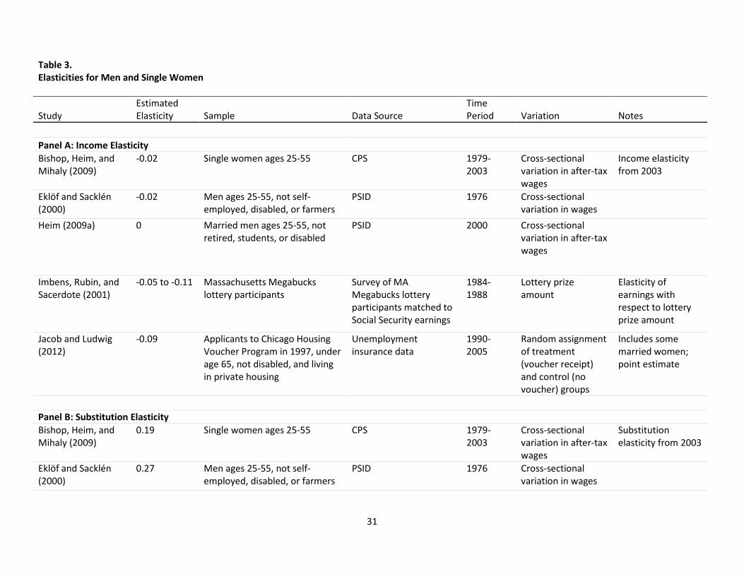
Sacerdote (2001) use data on lottery winnings and estimate income elasticities of wage income between
-0.05 and -0.11, and Jacob and Ludwig (2012) use a randomized lottery for housing vouchers and
estimate an income elasticity of hours worked by members of lower-income households who apply for
housing assistance of -0.09. Using recent survey data, Bishop, Heim, and Mihaly (2009) and Heim
(2009a) find income elasticities close to zero for single women and married men. For working-age men,
Eklöf and Sacklén (2000) also estimate an income elasticity near zero. The results of those studies are
consistent with the range of estimated income elasticities between -0.1 and zero found in the earlier
CBO review.
Substitution Elasticity. In a recent survey of the literature on labor supply elasticities for men,
Keane (2011) cites only one study using a static model—Eklöf and Sacklén (2000)—that has been
published since CBO’s 1996 review (see Table 3, Panel B). Using a direct wage measure and examining
the impact of alternative sample restrictions and variable definitions, Eklöf and Sacklén estimate the
substitution elasticity to be 0.27 following the methods used by Hausman (1981). Heim (2009a)
estimates the substitution elasticity for married men to be in the range of 0.04 to 0.07. Other recent
studies (Bishop, Heim, and Mihaly, 2009, and Jacob and Ludwig, 2012) estimate elasticities to be about
0.2. Considering all of the evidence, we conclude that the range encompassing most estimates extends
from 0.1 to 0.3 (a range with a higher upper end than that of the 0.1 to 0.2 range reported in CBO’s 1996
review).
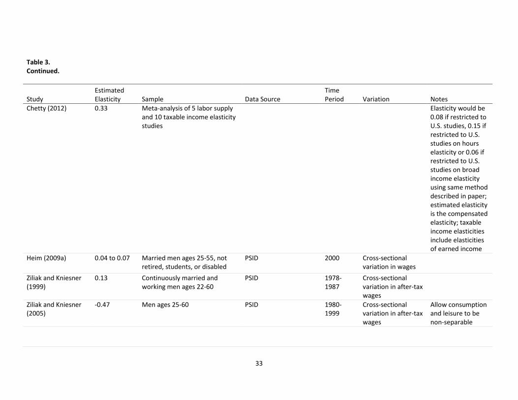
Elasticities of Participation and Hours Worked. Ziliak and Kniesner (1999) estimate an hours
elasticity of 0.13 for married men ages 21 to 61 (see Table 3, Panel C). In a later study (2005) that uses
more years of data, they estimate an elasticity of -0.47. Unlike many of the other studies included in this
review, these studies make strong assumptions about preferences and life-cycle effects. They also
include different control variables than most other papers. The unusually large and negative estimated
elasticity could be the result of those differences.
16
Chetty (2012) finds an average participation elasticity of 0.25 (see Table 3, Panel D). This
estimate includes participation elasticities of married women and single mothers who are the target of
EITC expansions and welfare reform; elasticities of that group tend to be higher than those of the
general population of men and single women. Juhn, Murphy, and Topel (2002) estimate participation
elasticities between 0.05 and 0.29 for men stratified by income group, with a population-weighted
average of 0.13. Bishop, Heim, and Mihaly (2009) find that the hours and participation elasticities for
single women fell between 1979 and 2003. Over the period 1996 through 2003, the estimated hours
elasticities varied from about 0.10 to -0.03, and the estimated participation elasticities varied from
about 0.1 to 0.2. The hours elasticities are within the range reported in other studies for men, while the
participation elasticities are slightly higher. For married men, Heim (2009a) finds no response of
participation and elasticities ranging from 0.04 to 0.07 for hours.
In the prior subsections, we extended the upper bound on substitution elasticities from 0.2 in
the 1996 review to 0.3 in order to incorporate a new estimate but did not changed the range of income
elasticities from the 1996 review. That extension of the range of substitution elasticities would be
reflected in either higher hours elasticities or higher participation elasticities. However, labor force
participation rates for this population are already high, leaving little room for an increase, and most men
and single women have little ability to cease working while maintaining a satisfactory income.
Consequently, we assume that the increase in the total reflects an increase in the hours elasticity. We
therefore raise the upper bound on the hours elasticity by 0.1 relative to CBO’s 1996 review, producing
a range for the hours elasticity of -0.1 to 0.2. The recent literature estimates participation elasticities
ranging from zero to 0.1 for men (for example, see Heim 2009a and Juhn, Murphy, and Topel 2002).
Although one paper reports an estimated elasticity for single women that is higher (Bishop, Heim, and
Mihaly 2009), the difference is not enough to justify changing the combined elasticity for men and single
17
women. We therefore conclude that the range of zero to 0.1 from CBO’s 1996 review still summarizes
the literature about the participation elasticity.
Elasticities for Married Women
The growth in women’s labor force participation in recent decades has motivated a number of
papers examining the labor supply elasticities for married women. Heim (2007) presents convincing
evidence that changes in women’s age profile and education levels are responsible for declines in their
labor supply elasticities between 1979 and 2003, but the magnitudes of the declines are not clear.9 Blau
and Kahn (2007) find similar declines in labor supply elasticities using cross-sectional wage variation in
three periods between 1979 and 2001, although their point estimates of the elasticities differ from
Heim’s estimates.
Income Elasticity. Research shows that income elasticities of married women are small in
magnitude. Blau and Kahn (2007) and Heim (2007) find income elasticities of about -0.1 (see Table 4,
Panel A). Jacob and Ludwig (2012) include married women in their sample; their estimates of -0.09 are
consistent with the elasticities estimated using survey data restricted to married women. Thus, the
recent literature suggests income elasticities of -0.1 for this group.10 However, because married
women’s labor supply elasticities are declining and therefore becoming more similar to those of men
and single women, we assume the range of income elasticities for married women matches that
discussed above for men and single women—namely, -0.1 to zero.
9 Heim’s estimates are derived from regression analysis on point elasticities estimated for each year using a combination of instrumental variables and sample selection models. The precision of the estimated point elasticities depends on the strength of the instruments, and the high year-to-year variation in the elasticities may arise because the instruments used are not very strong. It is not clear that using regression analysis on those points is an appropriate procedure for increasing the precision of the estimates. 10 Kumar (2012) estimates income elasticities for married women between -0.4 and -0.6 using 1986 tax reforms for identification. As demonstrated in Heim (2007), married women’s labor supply elasticities have sharply declined since that time. Thus, those estimates are not included in our range of elasticities for married women.
18
Substitution Elasticity. Blau and Kahn (2007) estimate that the total elasticity of hours worked
by married women with respect to after-tax wages fell from 0.7 between 1979 and 1981 to 0.3 or 0.4
between 1999 and 2001 (see Table 4, Panel B).11 Heim (2007) also finds a sharp decline in the
substitution elasticity and estimates a value of about 0.2, representing an hours response of 0.14 and a
participation response of 0.03. Using an estimation approach that assumes a quadratic utility function,
Heim (2009a) finds substitution elasticities of about 0.3. Thus, based on the recent literature,
substitution elasticities appear to range from 0.2 to 0.4.
Elasticities of Participation and Hours Worked. For married women, Heim (2009a) estimates
that the elasticity of hours worked with respect to wages is between 0.2 and 0.3 and that the elasticity
of participation with respect to wages is 0.1 and 0.2 (see Table 4, Panels C and D). Although the study
specifies the utility function of workers, it finds a range of elasticities that is not very different from
those found in other studies. Heim (2007) also distinguishes between income and substitution
elasticities for both the hours and participation responses. For hours worked, he estimates that
substitution elasticities decreased from 0.36 to 0.14 and income elasticities fell from -0.05 to -0.02
between 1978 and 2002 (elasticities from 1978 are not shown in the table); for participation, over this
time period income elasticities fell from -0.13 to -0.05, while substitution elasticities fell from 0.66 to
0.03.12 If substitution effects dominate income effects, as suggested by significant amounts of other
research, the hours and participation elasticities should be somewhat close to the substitution
components of those elasticities. The hours elasticity would then be 0.1, and the participation elasticity
would be zero, and those values form our lower bounds. While we find no evidence that would lead to
11 Studies of women’s labor supply differ on how education and fertility are modeled. If women who prefer fewer children also tend to earn higher wages and have a higher labor supply, then omitting the number of children as an explanatory variable can result in a spurious positive correlation between wages and labor supply. If, however, fertility is influenced by wages (for example, if higher wages induce women to work more and have fewer children), then controlling for the number of children will understate the total effect of wages on labor supply. 12 Because Heim does not report the ratio of labor income to nonlabor income, we cannot calculate the corresponding participation and hours elasticities.
19
changes in the upper bounds on hours elasticities, Blau and Kahn (2007) effectively demonstrate that
the upper bound on the participation elasticity has fallen to 0.3. Therefore, our ranges for hours and
participation elasticities for married women are 0.1 to 0.3 and zero to 0.3, respectively.
Elasticity of Broad Income
The range of estimates of the elasticity of broad income is similar to the range of estimates of
the elasticity of labor supply from the traditional labor supply literature. As discussed above, the
elasticity of broad income has some advantages and disadvantages relative to the elasticity of hours
worked as a measure of the responsiveness of labor supply. However, we interpret the similarity of the
ranges of estimates as supporting the ranges we identified in the previous sections of this review.
Income Elasticity. In this literature, the income elasticity is generally assumed to be zero (for
example, see Saez, 2004, and Saez, Slemrod, and Giertz, 2012). A few studies that distinguish income
elasticities (for example, see Kopczuk, 2005, and Gruber and Saez, 2002) estimate that the income
elasticity is small and insignificantly different from zero. Using Social Security earnings records matched
to survey data for lottery participants, Imbens, Rubin, and Sacerdote (2001) estimate income elasticities
ranging from -0.05 to -0.11, which is still quite small. Therefore, we interpret estimates of the elasticity
of broad income as substitution elasticities.
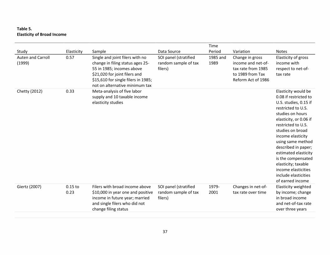
Substitution Elasticity. Broad income elasticities estimated using tax returns generally range
between zero and 0.3 (see Table 5). Gruber and Saez (2002) estimate that the elasticity of broad income
with respect to the net-of-tax rate is between 0.07 and 0.12 using three-year changes over the period
1979 through 1990, while Giertz (2007) estimates that this elasticity is between 0.15 and 0.23 using a
different dataset and including an additional decade—marked by significant changes in tax law—of data.
Additional studies using data spanning fewer years find similar elasticities—0.1 (Saez, 2003) and 0.2
(Heim, 2009b). Two studies, Kopczuk (2005) and Giertz (2010), form both the lower and upper bounds of
the range we identify. Both studies find a lower bound of about zero, with Giertz’s estimate reflecting
20
the short-term response of hours to a permanent change in tax rates, and both find an upper bound of
about 0.3. This range encompasses the range of substitution elasticities found in the traditional labor
supply literature for men and single women and is on the lower end of that range for married women.
Elasticities can depend on the length of time over which the response is measured. On one
hand, as noted above, workers may be better able to change their work hours or labor force
participation over a longer period of time. On the other hand, changes in the timing of income can result
in a higher responsiveness of taxable income to changes in net-of-tax rates over short periods of time.
Estimates outside the range from zero to 0.3 that we identify appear to be attributable to income timing
by high-income taxpayers (see Goolsbee, 2000) or to short-term income shifting around a major tax
change (see Auten and Carroll, 1999).13
Role of Frictions. Chetty (2012) reconciles the wide range of estimated substitution elasticities
by introducing a role for frictions. He argues that the observed response to tax changes can differ from
the true substitution elasticity because of frictions in the labor market; those frictions can be thought of
as adjustment costs or price misperceptions. Chetty derives bounds on a true elasticity using the tax
change, the observed elasticity, and an exogenously determined magnitude of frictions (expressed as
the percentage of earnings lost from not working the optimal number of hours). When there are
multiple observed estimates of an elasticity, a point estimate of the true elasticity can be derived by
finding the minimum amount of frictions that generates bounds consistent with the observed estimates.
In his meta-analysis pooling five studies using hours data and ten studies using tax return data,
Chetty calculates a long-run true substitution elasticity for hours worked by people in the labor force
13 Saez, Slemrod, and Giertz (2012) point out that using only two years of data when tax-rate changes are concentrated in one portion of the income distribution can lead to unconvincing results. Auten and Carroll (1999) show that using two years of data can lead to estimates that are very sensitive to specification choices.
21
with respect to net-of-tax rates of 0.33 (see Table 5).14 Although income should be more sensitive to
taxes than are hours worked, for the reasons discussed above, the average elasticity of income and the
average elasticity of hours are both 0.15 among the studies analyzed by Chetty.15
The studies used by Chetty to bound the elasticity for hours worked by people in the labor force
examine responses to tax changes in the United States, Sweden, the United Kingdom, Iceland, and
Denmark. The size of the tax changes studied varied greatly among the five countries, with Iceland and
Sweden experiencing substantially larger rate changes than the other three countries. Because the costs
of adjusting labor supply are probably smaller relative to the potential gains (that is, the frictions are
probably less important) in the countries with the larger rate changes, Chetty asserts that the observed
elasticities for Iceland and Sweden are closer to the true elasticity. However, institutional differences in
tax systems and labor markets in these countries may also lead to higher elasticities. For example,
because health insurance in Sweden is not tied to full-time employment, the average number of hours
worked may be more sensitive to changes in after-tax wage rates. If we consider only the studies used
by Chetty that examine responses to tax changes in the United States, the derived true elasticity for
hours worked by people in the labor force drops sharply from 0.33 to 0.08, while the average elasticity
of hours falls slightly from 0.15 to 0.12. Nevertheless, it is reasonable to believe that labor market
frictions mean that estimated elasticities of labor supply are biased downward to some extent. The
range of elasticities in the long run is therefore likely to exceed the range of elasticities that has been
estimated for the U.S. economy.
14 Chetty (2012) and Chetty et al. (2012) also examine the possible role of frictions in estimates of the participation elasticity in the traditional labor supply literature. They conclude that frictions would have to be implausibly large to explain the differences among those estimates, so those differences probably reflect differences in the true elasticities of the groups being studied. 15 The estimates of taxable income elasticities used by Chetty (2012) also include studies using earned income.
22
Elasticities by Income Group
Labor supply elasticities may differ by income group (see Juhn, Murphy, and Topel, 2002, and
Ziliak and Kniesner, 1999). If, for example, lower-income people have lower labor force participation
rates, then their participation response to reductions in tax rates could be higher because there are
more people who could enter the workforce. And if elasticities vary by income, then tax policies that
target lower-income taxpayers may produce different labor supply responses than policies that target
higher-income taxpayers. Therefore, it is inappropriate to use the ranges of elasticities presented in
Table 2 as estimates for the changes in labor supply that would result from all potential changes in tax
policies.
High-Income Individuals. Several studies use tax-return data to examine the elasticity of broad
income among high-income taxpayers. Compared to survey data, the tax data used in these studies
oversample high-income taxpayers, so sample sizes are larger. Relative to other taxpayers, high-income
taxpayers typically have more non-wage and salary income and more opportunities to reduce taxation
by shifting income from year to year or from taxed sources to untaxed (or more lightly taxed) sources.
Therefore, the responsiveness of broad income is probably less reflective of the labor supply response
for high-income individuals than for other individuals, and in particular the estimated elasticity of broad
income for high-income individuals probably exceeds their labor supply elasticity.
For example, Saez (2004) notes that although the elasticity of broad income among all taxpayers
is 0.2, the elasticity varies across income groups (see Table 6, Panel A). Among the top 1 percent of
taxpayers, a 1 percentage-point increase in the net-of-tax rate increases broad income by 0.5
percentage points, but among the bottom 99 percent of taxpayers, a similar increase in the net-of-tax
rate has a very small (and imprecisely estimated) effect on broad income. Heim (2009b) finds an even
greater elasticity of 0.7 to 0.9 for taxpayers with incomes above $500,000 in the base year, while his
estimates of elasticities for other taxpayers are close to zero and imprecisely estimated.
23
There have been several attempts to abstract from other sorts of responses by high-income
taxpayers in order to focus on their labor supply responses. Showalter and Thurston (1997) use survey
data of self-employed physicians to estimate the elasticity of physicians’ hours; their estimated elasticity
of 0.33 is higher than many estimates for other groups. Goolsbee (2000) uses the Execucomp database
to examine the taxable income elasticities of executives. While estimated short-run elasticities (which
incorporate income shifting) exceed 1, estimated longer-run elasticities vary from -0.17 to 0.40. The
estimated short-run elasticities for executives with incomes over $1 million exceed 2, mostly due to
shifts in the timing of compensation and especially the choice of when to exercise stock options, and
executives with incomes between $275,000 and $500,000 have short-run elasticities less than 0.4. The
estimated long-run elasticities show a similar pattern across income levels: 0.55 for executives with
incomes over $1 million and 0.34 for those with incomes between $275,000 and $500,000.
Furthermore, the estimated short-run and long-run elasticities for salary and bonuses are relatively low:
0.15 and 0.09, respectively. In sum, with the exception of executives with incomes in excess of
$1 million, the elasticities of executives’ labor supply and wage income are barely outside the ranges of
elasticities presented in Table 2.
Low-Income Individuals. Juhn, Murphy, and Topel (2002) estimate participation elasticities for
men at different points in the wage distribution using cross-sections of the Current Population Survey.
They find that participation elasticities are largest at the lower end of the distribution—for example, the
estimated participation elasticity for workers in the bottom 10 percent of the wage distribution is more
than twice as large as that for workers near the middle of the distribution.
A number of studies have used the variation in after-tax wage rates created by the expansion of
the EITC to estimate the labor supply response among low-income workers. Eissa and Hoynes (2006)
review the research on the effect of the EITC on labor supply. They find that studies consistently show a
statistically significant link between expansions of the EITC and increases in labor force participation
24
among single mothers. However, those studies have not found evidence that those expansions cause
people already in the work force to change the number of hours they worked. The consistency of those
findings is notable, occurring across studies using different policy changes, control groups, and
methodologies.
There are a few possible explanations for the lack of a statistically significant effect of changes in
the EITC on how many hours people work. The first possible explanation is that the true effect is weak.
Indeed, a number of studies find that the labor supply elasticity of working women is lower than the
elasticity of all women (for example, see Mroz, 1987, and Triest, 1990). Another possible explanation is
that the estimates are imprecise. Many of the studies use quasi-experimental or semi-parametric
approaches that, because they impose fewer restrictions on the form of the relationship between after-
tax wages and hours worked, generally result in less precise estimates than parametric approaches; also,
the variable of interest—hours worked—is imprecisely measured. A final possible explanation is that,
while the EITC as a refundable tax credit for low-income workers is well-publicized, the marginal tax
rates associated with the phase-in and phaseout ranges are probably less well known and are obscured
by interactions with other tax provisions. If EITC recipients do not recognize the incentives created by
changes in the EITC, then they would not change their labor supply in response. Recent work by Chetty,
Friedman, and Saez (2012) using tax return data suggests that almost all of the labor supply response to
the EITC comes from workers in the phase-in region. In contrast to most of the previous literature, they
find that the most of the increase in EITC refunds is due to increases in wages among individuals who are
already working; the estimated elasticity of participation is smaller than the estimated elasticity of hours
worked.
On the participation margin for low-income individuals, Hotz and Scholz (2003) find elasticities
with respect to after-tax income ranging from 0.69 to 1.16 in their review of the literature (see Table 6,
Panel B). Using variation in wages from expansions of the EITC and means-tested transfers, Meyer and
25
Rosenbaum (2001) estimate that, for single mothers, the elasticity of working during the year with
respect to after-tax wages is 0.4. Eissa and Hoynes (2004) use data from 1984 to 2006 to examine the
effect of the EITC on participation rates for married couples with children. The authors estimate that the
total elasticity of participation by married women with respect to after-tax wages is 0.27, while the
participation elasticity for husbands is only 0.03. The authors also estimate that a $1,000 increase in net
unearned income reduces the participation of wives by 0.1 percentage points and of husbands by
0.5 percentage points, implying income elasticities of -0.04 and -0.01, respectively.
Estimates of the elasticity of participation from the EITC literature are generally higher than
those estimated for groups not eligible for the EITC, which is consistent with the higher estimated
elasticities found by Juhn, Murphy, and Topel (2002). For comparison, Blau and Kahn (2007) estimate
participation elasticities with respect to wages ranging from 0.27 to 0.30 among married women. The
higher elasticities found in the EITC literature may reflect the lower initial labor force participation of
lower-income single women with children, the focus of a number of EITC studies.
26
References
Auten, Gerald, and Robert Carroll. 1999. “The Effect of Income Taxes on Household Income,“ Review of Economics and Statistics, 81 (4): 681-693. Bishop, Kelly, Bradley Heim, and Kata Mihaly. 2009. “Single Women’s Labor Supply Elasticities: Trends and Policy Implications,” Industrial and Labor Relations Review, 63 (1): 146-168. Blau, Francine D., and Lawrence M. Kahn. 2007. “Changes in the Labor Supply Behavior of Married Women: 1980-2000,” Journal of Labor Economics, 25, 393-438. Chetty, Raj. 2012. “Bounds on Elasticities with Optimization Frictions: A Synthesis of Micro and Macro Evidence on Labor Supply,” Econometrica, 80 (3): 969-1018. Chetty, Raj, John Friedman, and Emmanuel Saez. 2012. “Using Differences in Knowledge Across Neighborhoods to Uncover the Impacts of the EITC on Earnings,” National Bureau of Economic Research Working Paper 18232. Chetty, Raj, Adam Guren, Day Manoli, and Andrea Weber. “Does Indivisible Labor Explain the Difference Between Micro and Macro Elasticities? A Meta-Analysis of Extensive Margin Elasticities,” National Bureau of Economic Research Macroeconomics Annual, 2012. Congressional Budget Office. 1996. Labor Supply and Taxes. CBO Memorandum, www.cbo.gov/publication/13598. Davis, Stephen J., and Magnus Henrekson. 2005. “Tax Effects on Work Activity, Industry Mix and Shadow Economy Size: Evidence from Rich Country Comparisons,” in Labour Supply and Incentives to Work in Europe, R. Gómez-Salvador, A. Lamo, B. Petrongolo, M. Ward, E. Wasmer, eds., 44-104. Eissa, Nada, and Hilary W. Hoynes. 2006. “Behavioral Responses to Taxes: Lessons from the EITC and Labor Supply,” Tax Policy and the Economy, vol. 20, James M. Poterba, ed. Eissa, Nada, and Hilary W. Hoynes. 2004. “Taxes and the Labor Market Participation of Married Couples: The Earned Income Tax Credit,” Journal of Public Economics, 88 (2004): 1931-1958. Eklöf, Matias, and Hans Sacklén. 2000. “The Hausman-MaCurdy Controversy: Why Do the Results Differ Across Studies?” Journal of Human Resources, 35 (1): 204-220. Giertz, Seth. 2007. “The Elasticity of Taxable Income over the 1980s and 1990s,” National Tax Journal, 60 (4): 743-768. Giertz, Seth. 2010. “The Elasticity of Taxable Income during the 1990s: New Estimates and Sensitivity Analyses,” Southern Economic Journal, 77 (2): 406-433. Goolsbee, Austan. 2000. “What Happens When You Tax the Rich? Evidence from Executive Compensation,” Journal of Political Economy, 108 (2): 352-378.
Gruber, Jonathan, and Emmanuel Saez. 2002. “The Elasticity of Taxable Income: Evidence and Implications,” Journal of Public Economics, 84, 1-32. Hausman, Jerry A., 1981. “Labor Supply,” How Taxes Affect Economic Behavior, Henry J. Aaron and Joseph Pechman, eds., 27-83. Heim, Bradley. 2007. “The Incredible Shrinking Elasticities: Married Female Labor Supply, 1978-2002,” Journal of Human Resources, 42 (4): 881-918. Heim, Bradley. 2009a. “Structural Estimation of Family Labor Supply with Taxes: Estimating a Continuous Hours Model Using a Direct Utility Specification,” Journal of Human Resources, 44 (2): 350-385. Heim, Bradley. 2009b. “The Effect of Recent Tax Changes on Taxable Income: Evidence from a New Panel of Tax Returns,” Journal of Policy Analysis and Management, 28 (1): 147-163. Hotz, V. Joseph, and John Karl Scholz. 2003. “The Earned Income Tax Credit,” Means-Tested Transfer Programs in the U.S., R. Moffitt, ed., Chicago: University of Chicago Press, 141-198. Imbens, Guido W., Donald B. Rubin, and Bruce I. Sacerdote. 2001. “Estimating the Effect of Unearned Income on Labor Earnings, Savings, and Consumption: Evidence from a Survey of Lottery Players,” American Economic Review, 91 (4): 778-794. Jacob, Brian A., and Jens Ludwig. 2012. “The Effects of Housing Assistance on Labor Supply: Evidence from a Voucher Lottery,” American Economic Review, 102 (1): 272-304. Juhn, Chinhui, Kevin M. Murphy, and Robert H. Topel. 2002. “Current Unemployment, Historically Contemplated,” Brookings Papers on Economic Activity, 2002 (1): 79-116. Keane, Michael P. 2011. “Labor Supply and Taxes: A Survey,” Journal of Economic Literature, 2011, 49 (4): 961-1075. Kopczuk, Wojciech. 2005. “Tax Bases, Tax Rates and the Elasticity of Reported Income," Journal of Public Economics, 89, 2093-2119. Kumar, Anil. 2012. “Nonparametric Estimation of the Impact of Taxes on Female Labor Supply,” Journal of Applied Econometrics, 27: 415-439. Ljungqvist, Lars, and Thomas J. Sargent. 2011. “A Labor Supply Elasticity Accord?” American Economic Review, 101 (3): 487-491. MaCurdy, Thomas, David Green, and Harry Paarsch. 1990. "Assessing Empirical Approaches for Analyzing Taxes and Labor Supply," Journal of Human Resources, 25 (3): 415-490. Meyer, Bruce D., and Dan T. Rosenbaum. 2001. “Welfare, the Earned Income Tax Credit, and the Labor Supply of Single Mothers,” Quarterly Journal of Economics, 116 (3): 1063-1114. Mroz, Thomas A. 1987. “The Sensitivity of an Empirical Model of Married Women’s Hours of Work to Economic and Statistical Assumptions,” Econometrica, 55 (4): 765-799.
Prescott, Edward C. 2003. “Why Do Americans Work So Much More Than Europeans?” Federal Reserve Bank of Minneapolis Research Department Staff Report 321. Prescott, Edward C. 2006. “Nobel Lecture: The Transformation Macroeconomic Policy and Research.” Journal of Political Economy, 114 (2): 203-235. Saez, Emmanuel. 2003. “The Effect of Marginal Tax Rates on Income: A Panel Study of ‘Bracket Creep,’” Journal of Public Economics, 87: 1231-1258. Saez, Emmanuel. 2004. “Reported Incomes and Marginal Tax Rates, 1960-2000: Evidence and Policy Implications,” National Bureau of Economic Research Working Paper 10273. Saez, Emmanuel, Joel Slemrod, and Seth Giertz. 2012. “The Elasticity of Taxable Income with Respect to Marginal Tax Rates: A Critical Review,” Journal of Economic Literature, 50 (1): 3-50. Showalter, Mark H., and Norman K. Thurston. 1997. “Taxes and Labor Supply of High-Income Physicians,” Journal of Public Economics, 66 (1997): 73-97. Triest, Robert K. 1990. “The Effect of Income Taxation on Labor Supply in the United States,” The Journal of Human Resources, 25 (3): 491-516 Ziliak, James P., and Thomas J. Kniesner. 2005. "The Effect of Income Taxation on Consumption and Labor Supply," Journal of Labor Economics, 23 (4): 769-796. Ziliak, James P., and Thomas J. Kniesner. 1999. "Estimating Life Cycle Labor Supply Tax Effects," Journal of Political Economy, 107 (2): 326-359.
29
Table 1. Summary of Labor Supply Elasticities from CBO’s 1996 Review
Broken Down into Broken Down into
Total Wage Income Substitution Average-Hours Participation
Men -0.1 to 0.2 -0.1 to 0 0.1 to 0.2 -0.1 to 0.1 0 to 0.1 Married Women 0.3 to 0.7 -0.3 to -0.2 0.6 to 0.9 0.1 to 0.3 0.2 to 0.4 All People 0 to 0.3 -0.2 to -0.1 0.2 to 0.4 -0.1 to 0.1 0.1 to 0.2 SOURCE: Congressional Budget Office. 1996. “Labor Supply and Taxes.” CBO Memorandum, www.cbo.gov/publication/13598.
Table 2. Updated Ranges of Labor Supply Elasticities
Panel A. Income and Substitution Elasticities
Income Substitution
Men and Single Women -0.1 to 0 0.1 to 0.3
Married Women -0.1 to 0 0.2 to 0.4
Total Population -0.1 to 0 0.1 to 0.3
Panel B. Hours and Participation Elasticities
Hours Participation
Men and Single Women -0.1 to 0.2 0 to 0.1
Married Women 0.1 to 0.3 0 to 0.3
Total Population 0 to 0.2 0 to 0.2
31
Table 3. Elasticities for Men and Single Women
Study Estimated Elasticity Sample Data Source
Time Period Variation Notes
Panel A: Income Elasticity Bishop, Heim, and Mihaly (2009)
-0.02 Single women ages 25-55 CPS 1979-2003
Cross-sectional variation in after-tax wages
Income elasticity from 2003
Eklöf and Sacklén (2000)
-0.02 Men ages 25-55, not self-employed, disabled, or farmers
PSID 1976 Cross-sectional variation in wages
Heim (2009a) 0 Married men ages 25-55, not retired, students, or disabled
PSID 2000 Cross-sectional variation in after-tax wages
Imbens, Rubin, and Sacerdote (2001)
-0.05 to -0.11 Massachusetts Megabucks lottery participants
Survey of MA Megabucks lottery participants matched to Social Security earnings
1984-1988
Lottery prize amount
Elasticity of earnings with respect to lottery prize amount
Jacob and Ludwig (2012)
-0.09 Applicants to Chicago Housing Voucher Program in 1997, under age 65, not disabled, and living in private housing
Unemployment insurance data
1990-2005
Random assignment of treatment (voucher receipt) and control (no voucher) groups
Includes some married women; point estimate
Panel B: Substitution Elasticity Bishop, Heim, and Mihaly (2009)
0.19 Single women ages 25-55 CPS 1979-2003
Cross-sectional variation in after-tax wages
Substitution elasticity from 2003
Eklöf and Sacklén (2000)
0.27 Men ages 25-55, not self-employed, disabled, or farmers
PSID 1976 Cross-sectional variation in wages
32
Table 3. Continued.
Study Estimated Elasticity Sample Data Source
Time Period Variation Notes
Heim (2009a) 0.04 to 0.07 Married men ages 25-55, not retired, students, or disabled
PSID 2000 Cross-sectional variation in wages
Jacob and Ludwig (2012)
0.15 Applicants to Chicago Housing Voucher Program in 1997, under age 65, not disabled, and living in private housing
Unemployment insurance data
1990-2005
Random assignment of treatment (voucher receipt) and control (no voucher) groups
Includes some married women; point estimate
Keane (2011) 0.05 to 0.84 Men Literature review of static models
Panel C: Hours Elasticity Bishop, Heim, and Mihaly (2009)
-0.03 (substitution) -0.02 (income)
Single women ages 25-55 CPS 1979-2003
Cross-sectional variation in after-tax wages
Substitution elasticity from 2003
33
Table 3. Continued.
Study Estimated Elasticity Sample Data Source
Time Period Variation Notes
Chetty (2012) 0.33 Meta-analysis of 5 labor supply and 10 taxable income elasticity studies
Elasticity would be 0.08 if restricted to U.S. studies, 0.15 if restricted to U.S. studies on hours elasticity or 0.06 if restricted to U.S. studies on broad income elasticity using same method described in paper; estimated elasticity is the compensated elasticity; taxable income elasticities include elasticities of earned income
Heim (2009a) 0.04 to 0.07 Married men ages 25-55, not retired, students, or disabled
PSID 2000 Cross-sectional variation in wages
Ziliak and Kniesner (1999)
0.13 Continuously married and working men ages 22-60
PSID 1978-1987
Cross-sectional variation in after-tax wages
Ziliak and Kniesner (2005)
-0.47 Men ages 25-60 PSID 1980-1999
Cross-sectional variation in after-tax wages
Allow consumption and leisure to be non-separable
34
Table 3. Continued.
Study Estimated Elasticity Sample Data Source
Time Period Variation Notes
Panel D: Participation Elasticity Bishop, Heim, and Mihaly (2009)
0.22 (substitution) 0 (income)
Single women ages 25-55 CPS 1979-2003
Cross-sectional variation in after-tax wages
Substitution elasticity from 2003
Chetty (2012) 0.25 Average among labor supply studies estimating participation elasticities
Literature review Average would be 0.24 if restricted to U.S. studies; includes studies of married women
Heim (2009a) 0 Married men ages 25-55, not retired, students, or disabled
PSID 2000 Cross-sectional variation in wages
Juhn, Murphy, and Topel (2002)
0.05 to 0.29, weighted average of 0.13
Working-age men March CPS 1972-1973 and 1988-1989
Change in participation rate from cross-sectional wage variation
Note: CPS=Current Population Survey; PSID=Panel Study of Income Dynamics.
35
Table 4. Elasticities for Married Women
Study Elasticity Sample Data Source Time Period Variation Notes
Panel A: Income Elasticity Blau and Kahn (2007)
-0.1 to -0.14 Married women ages 25-54 with spouse ages 25-54
March CPS 1999-2001
Net-of-tax wage rate
Heim (2007) -0.05 (participation) -0.02 (hours)
Married women ages 25-55, not self-employed, retired, disabled, or students
March CPS 1979-2003
Cross-sectional variation in wages
Elasticity estimates for 2002; population-weighted
Jacob and Ludwig (2012)
-0.09 Applicants to Chicago Housing Voucher Program in 1997, under age 65, not disabled, and living in private housing
Unemployment insurance data
1990-2005
Random assignment of treatment (voucher receipt) and control (no voucher) groups
Includes some men and single women; point estimate
Kumar (2009) -0.4 to -0.7 Married women ages 25-60, not self-employed, not in SEO subsample
PSID 1985 and 1989
1986 tax reform
Panel B: Substitution Elasticity Blau and Kahn (2007)
0.33 to 0.38 Married women ages 25-54 with spouse ages 25-54
March CPS 1999-2001
Net-of-tax wage rate
Population-weighted estimates
Heim (2007) 0.03 (participation) 0.14 (hours)
Married women ages 25-55, not self-employed, retired, disabled, or students
March CPS 1979-2003
Cross-sectional variation in wages
Elasticity estimates for 2002; population-weighted
Heim (2009a) 0.25 to 0.34 Married women with husband ages 25-55, not retired, disabled, student, or working more than 4,000 hours a year
PSID 2000 Cross-sectional variation in after-tax wages
36
Table 4. Continued.
Study Elasticity Sample Data Source Time Period Variation Notes
Jacob and Ludwig (2012)
0.15 Applicants to Chicago Housing Voucher Program in 1997, under age 65, not disabled, and living in private housing
Unemployment insurance data
1990-2005
Random assignment of treatment (voucher receipt) and control (no voucher) groups
Includes some men and single women; point estimate
Kumar (2009) 0.3 to 0.7 Married women ages 25-60, not self-employed, not in Survey of Economic Opportunity subsample
PSID 1985 and 1989
1986 tax reform
Panel C: Hours Elasticity Blau and Kahn (2007)
0.10 to 0.12 Married women ages 25-54 with spouse ages 25-54
March CPS 1999-2001
Cross-sectional wage variation
Heim (2007) 0.14 (substitution) -0.02 (income)
Married women ages 25-55, not self-employed, retired, disabled, or students
March CPS 1979-2003
Cross-sectional variation in wages
Elasticity estimates for 2002; population-weighted
Heim (2009a) 0.24 to 0.33 (substitution)
Married women with husband ages 25-55, not retired, disabled, student, or working more than 4,000 hours a year
PSID 2000 Cross-sectional variation in after-tax wages
Panel D: Participation Elasticity Blau and Kahn (2007)
0.27 to 0.29 Married women ages 25-54 with spouse ages 25-54
March CPS 1999-2001
Cross-sectional wage variation
Heim (2007) 0.03 (substitution) -0.05 (income)
Married women ages 25-55, not self-employed, retired, disabled, or students
March CPS 1979-2003
Cross-sectional variation in wages
Elasticity estimates for 2002; population-weighted
Heim (2009a) 0.07 to 0.17 (substitution)
Married women with husband ages 25-55, not retired, disabled, student, or working more than 4,000 hours a year
PSID 2000 Cross-sectional variation in after-tax wages
Note: CPS=Current Population Survey; PSID=Panel Study of Income Dynamics.
37
Table 5. Elasticity of Broad Income
Study Elasticity Sample Data Source Time Period Variation Notes
Auten and Carroll (1999)
0.57 Single and joint filers with no change in filing status ages 25-55 in 1985; incomes above $21,020 for joint filers and $15,610 for single filers in 1985; not on alternative minimum tax
SOI panel (stratified random sample of tax filers)
1985 and 1989
Change in gross income and net-of-tax rate from 1985 to 1989 from Tax Reform Act of 1986
Elasticity of gross income with respect to net-of-tax rate
Chetty (2012) 0.33 Meta-analysis of five labor supply and 10 taxable income elasticity studies
Elasticity would be 0.08 if restricted to U.S. studies, 0.15 if restricted to U.S. studies on hours elasticity, or 0.06 if restricted to U.S. studies on broad income elasticity using same method described in paper; estimated elasticity is the compensated elasticity; taxable income elasticities include elasticities of earned income
Giertz (2007) 0.15 to 0.23
Filers with broad income above $10,000 in year one and positive income in future year; married and single filers who did not change filing status
SOI panel (stratified random sample of tax filers)
1979-2001
Changes in net-of-tax rate over time
Elasticity weighted by income; change in broad income and net-of-tax rate over three years
38
Table 5. Continued.
Study Elasticity Sample Data Source Time Period Variation Notes
Giertz (2010) 0 to 0.1 (short term) 0.19 to 0.30 (long term)
Filed every year between 1989 and 1995 and taxable income above $10,000; married and single filers who did not change filing status
SOI panel 1988-1995
Changes in net-of-tax rate over time
Elasticity weighted by income
Goolsbee (2000) 1.3 in short run -0.17 to 0.4 in long run
Highest paid five employees of companies in Standard and Poor's S&P 500, S&P Midcap 400, and S&P Small Cap 600 in firms whose fiscal years end in December; individual observed at least four times
Execucomp 1991-1995
Change in net-of-tax-rate from 1993 tax act
Elasticity of broad income with respect to net-of-tax rate
Gruber and Saez (2002) 0.07 to 0.12 -0.07 income effect
Married and single filers without change in marital status; income above $10,000 in year one
CWHS (panel of tax returns from selecting certain four-digit endings of the primary taxpayer's Social Security number)
1979-1990
Change in net-of-tax rate over three-year period
Elasticity weighted by income; change in broad income and net-of-tax rate over three years; estimates vary depending on income controls used
Heim (2009b) 0.18 to 0.2 Filers over age 25 without change in filing status and gross income above $10,000 in 2000
Edited Panel of Tax Returns (CWHS + high-income sample from 1999)
1995-2004
Change in net-of-tax rate over three-year period
Imbens, Rubin, and Sacerdote (2001)
-0.05 to -0.11 (income elasticity)
Massachusetts Megabucks lottery participants
Survey of MA Megabucks lottery participants matched to Social Security earnings
1984-1988
Lottery prize amount
Elasticity of earnings with respect to lottery prize amount
39
Table 5. Continued.
Study Elasticity Sample Data Source Time Period Variation Notes
Kopczuk (2005) 0.01 to 0.31
Married filers; includes only filers without age exemption; no change in marital status; no head of household
SOI/University of Michigan tax panel
1979-1990
Changes in net-of-tax rate over three-year period (1980, 1986 tax reform)
Estimates for single filers less reliable; change in broad income and net-of-tax rate over three years; estimates vary across income groups; estimates unweighted
Saez (2003) 0.08 Single and married filers who do not change marital status and who are on regular tax schedule in year one
University of Michigan tax panel
1979-1981
Changes in net-of-tax rate over consecutive years
-0.44 for high income, 0.12 for middle income; estimates unweighted
Note: SOI=Statistics of Income, CWHS=Continuous Work History Sample.
40
Table 6. Elasticity by Income
Study Elasticity Sample Data Source Time Period Variation Notes
Panel A: High-Income Taxpayers
Goolsbee (2000) 1.3 in short run, -0.17 to 0.4 in long run
Highest paid five employees of companies in Standard and Poor's S&P 500, S&P Midcap 400, and S&P Small Cap 600 in firms whose fiscal years end in December; individual observed at least four times
Execucomp 1991-1995
Change in net-of-tax-rate from 1993 tax act
Elasticity of broad income with respect to net-of-tax rate
Heim (2009b) 0.67 to 0.90
Filers over age 25 without change in filing status and gross income above $500,000 in 2000
Edited Panel of Tax Returns (CWHS + high-income sample from 1999)
1995-2004
Change in net-of-tax rate over three-year period
Saez (2004) 0.2 Stratified sample of tax returns oversampled for high-income taxpayers
1960-2000
-0.04 for bottom 99 percent, 0.5 for top 1 percent
Elasticity of gross income net of capital gains and taxable Social Security and unemployment insurance benefits with respect to net-of-tax rate
Showalter and Thurston (1997)
0.33 Male physicians under age 60 with income above $80,000 in 1983 who are self-employed
Survey data from American Medical Association Master File of Physicians
1983-1987
Change in net-of-tax rate from 1986 tax reform and state tax variation
Elasticity of hours with respect to net-of-tax rate among workers
41
Table 6. Continued.
Study Elasticity Sample Data Source Time Period Variation Notes
Panel B: Low-Income Taxpayers
Eissa and Hoynes (2004)
0.03 Married men ages 25-54 with children and wife with less than 12 years of schooling
March CPS 1984-1996
Change in after-tax income from EITC expansions
Elasticity of labor force participation with respect to after-tax income
Eissa and Hoynes (2004)
0.27 Married women ages 25-54 with less than 12 years of schooling, with children
March CPS 1984-1996
Change in after-tax income from EITC expansions
Elasticity of labor force participation with respect to after-tax income
Hotz and Scholz (2003) 0.69 to 1.16
Single women with children Literature review Change in after-tax income from EITC expansions
Meyer and Rosenbaum (2001)
0.43 Single mothers ages 19-44 March CPS 1984-1996
Changes in after-tax wage from EITC expansions and means-tested transfers
Elasticity of labor force participation with respect to after-tax income
Note: CWHS=Continuous Work History Sample; CPS=Current Population Survey; EITC=earned income tax credit.