European Economic Review 31 (1987) 947-968. North-Holland A THEORY OF DYNAMIC OLIGOPOLY, III Cournot Competition Eric MASKIN* Harvard University, Cambridge, MA 02138, USA Jean TIROLE* Massachusetts Institute oJ Technology, Cambridge, MA 02139, USA We study the Markov perfect equilibrium (MPE) of an alternating move, infinite horizon duopoly model where the strategic variable is quantity. We exhibit a pair of difference- differential equations that, when they exist, differentiable MPE strategies satisfy. For quadratic payoff functions, we solve these equations in closed form and demonstrate that the MPE corresponding to the solution is the limit of the finite horizon equilibrium as the horizon tends to inlinity. We conclude with a discussion of adjustment costs and endogenization of the timing. 1. Introduction In Maskin andTirole (1982,1985), we presented a theory of how oligopolistic firms behave over time. We studied an explicitly temporal model stressing the idea of reactions based on short-run commitments. When we say that a firm is committed to a particular action, we mean that it cannot change that action for a certain finite (although possibly short) period, during which time other firms might act. By a firm’s reaction to another firm, we mean the response it makes, possibly after some lag, to the other’s chosen action. To formalize the ideas of commitment-based reactions, we introduced a class of infinite-horizon sequential duopoly games. In the simplest version of these games, the two firms move alternatingly. Thus, when a firm picks its action, it has perfect information about the current action of the rival. The fact that after choosing an action a firm cannot change it for two periods is meant to capture the idea of short-run commitment. A firm maximizes the present discounted value of its profits. Its strategy is assumed to depend only on the physical state of the system (i.e., to be Markov). In our model, the state is simply the other firm’s current action. Hence, a strategy is simply a dynamic reaction function. A Markov Perfect *We thank the NSF and the Sloan Foundation for research support. We are grateful to R.A. Dana and a referee for helpful comments. 00142921/87/$3.50 0 1987, Elsevier Science Publishers B.V. (North-Holland)
Transcript
European Economic Review 31 (1987) 947-968. North-Holland
A THEORY OF DYNAMIC OLIGOPOLY, III
Cournot Competition
Eric MASKIN*
Harvard University, Cambridge, MA 02138, USA
Jean TIROLE*
Massachusetts Institute oJ Technology, Cambridge, MA 02139, USA
We study the Markov perfect equilibrium (MPE) of an alternating move, infinite horizon duopoly model where the strategic variable is quantity. We exhibit a pair of difference- differential equations that, when they exist, differentiable MPE strategies satisfy. For quadratic payoff functions, we solve these equations in closed form and demonstrate that the MPE corresponding to the solution is the limit of the finite horizon equilibrium as the horizon tends to inlinity. We conclude with a discussion of adjustment costs and endogenization of the timing.
1. Introduction
In Maskin andTirole (1982,1985), we presented a theory of how oligopolistic firms behave over time. We studied an explicitly temporal model stressing the idea of reactions based on short-run commitments. When we say that a firm is committed to a particular action, we mean that it cannot change that action for a certain finite (although possibly short) period, during which time other firms might act. By a firm’s reaction to another firm, we mean the response it makes, possibly after some lag, to the other’s chosen action.
To formalize the ideas of commitment-based reactions, we introduced a class of infinite-horizon sequential duopoly games. In the simplest version of these games, the two firms move alternatingly. Thus, when a firm picks its action, it has perfect information about the current action of the rival. The fact that after choosing an action a firm cannot change it for two periods is meant to capture the idea of short-run commitment.
A firm maximizes the present discounted value of its profits. Its strategy is assumed to depend only on the physical state of the system (i.e., to be Markov). In our model, the state is simply the other firm’s current action. Hence, a strategy is simply a dynamic reaction function. A Markov Perfect
*We thank the NSF and the Sloan Foundation for research support. We are grateful to R.A. Dana and a referee for helpful comments.
948 E. Maskin and J. Tirole, A theory of dynamic oligopoly, III
Equilibrium (MPE) is a pair of reaction functions that form a perfect equilibrium. See section 2 below for a brief discussion and Maskin-Tirole (1982) for a more extended motivation of the MPE concept.
Maskin and Tirole (1982) applied this framework to a natural monopoly situation and provided a link between the older literature on fixed costs as an entry barrier and the more recent discussion of contestability. Maskin and Tirole (1985) examined dynamic price competition and developed equilibrium explanations for kinked demand curves, price cycles, excess capacity and market sharing.
In this paper, we adapt the alternating model to classic Cournot com- petition. Although we shall refer to a firm’s choosing a ‘quantity’, one should think of this choice as that of capital or capacity [cf. Kreps and Schienkman (1983) or Maskin and Tirole (1982)]. That is, the quantity-setting game is the reduced form of a more complicated game in which long-run competition is conducted through capital and short-run competition through prices.
Section 2 recalls our infinite horizon duopoly model with alternating moves and develops the first-order conditions for differentiable reaction functions to form a MPE. These lead to a pair of difference-differential equations in the two reaction functions. Payoff functions are thereafter assumed to be quadratic. Section 3 shows that, given the quadratic assump- tion, there exists a unique MPE with linear reaction functions. This equilibrium is dynamically stable. Moreover, when firms discount the future heavily, the equilibrium strategies coincide with standard Cournot reaction functions. However, as firms grow more patient, competition becomes increasingly intense.
In their pioneering contribution, Cyert and de Groot (1970) analyzed the finite horizon analogue of the model studied in this paper. Even in the quadratic case, the finite horizon equilibrium cannot be exhibited in closed form, and so Cyert and de Groot were compelled to use numerical methods to solve it. In section 4, we use a contraction mapping argument to show that, as the horizon lengthens, the finite horizon equilibrium strategies converge to their infinite horizon counterparts discussed in section 3. Thus, the nature of equilibrium is robust to the length of the horizon.
Section 5 alters the model by imposing a cost on a firm for changing its quantity. The cost is assumed to grow with the size of the change in output. In this case, we show that, for any discount factor, the steady-state equilibrium converges to the static Cournot outcome as adjustment costs become large.
One restrictive feature of our analysis is that it relies on a model where firms’ relative timing is exogenous. Both alternating and simultaneous move timings are, a priori, arbitrary. Asynchronism forces firms to react to one another; simultaneity, by contrast, does not permit reactions in our sense, since all firms commitments expire at the same time. In our previous papers,
E. Maskin and J. Tirole, A theory of dynamic oligopoly, 111 949
we argued that the timing of the game should not be imposed but instead result from the adjustment technology and the strategic interactions. In section 6 we discuss the issue of endogenous timing for the Cournot framework.
2. The model and Markov Perfect Equilibrium
In this section we describe the main features of the exogenous timing duopoly model [for further discussion of this model, see Maskin and Tirole (1982)]. Competition between the two firms (i= 1,2) takes place in discrete time with an infinite horizon. Time periods are indexed by t ( = 0, 1,2,. .). The time between two consecutive periods is 7: At time t, firm i’s instanta- neous profit ni is a function of the two firms’ current quantities (as we mentioned in the introduction, these quantities are really a ‘shorthand’ for
technological scale) ql, f and q2,t, but not of time: Z7i=17i(q,,,,q2.1). We
assume that ZZ’ is twice continuously differentiable, with nii ~0, lli<O and ZIij<O, where subscripts denote partial differentiation (for instance, Hij is the cross partial derivative of Z7 with respect to ql,t and q2,t). Thus, firm i’s profit is concave in i’s output and, like marginal profit, decreases with i’s competitor’s output. Static reaction curves are consequently well-defined and downward sloping.
Firms discount the future with the same interest rate r; thus, their discount factor is 6 =exp( --rT). Firm i’s intertemporal profit at time t is
f. 6”wq 1,r+sqz,t+s . 1
Let us now consider the timing of quantity setting. In odd-numbered periods t, firm 1 chooses its quantity, which remains unchanged until period
t+2. That is, ql,f+l=ql,f if t is odd. Similarly, firm 2 chooses quantities only in even-numbered periods, so that q2,t+ 1 = q2,1 if t is even.
Firm i’s strategy is assumed to depend only on the payoff-relevant state, those variables that directly enter its profit function. That is, we suppose that strategies are Markou. In period 2k+ 1, when it is firm l’s turn to pick a quantity, the payoff-relevant state is simply firm 2’s current output: q2, 2k+ 1 =
q2,2k. Firm l’s choice of quantity is, therefore, contingent only on q2,2k.
That is, its reaction function takes the form q1,2k+ 1 =R,(q,,,,). Similarly, firm 2 reacts to firm l’s quantity according to a reaction function R2(.), where q2,2k+2 =RZ(q1,2k+ 1). We shall call these Markov strategies dynamic
reaction functions. In this paper, we consider only deterministic reaction functions.
As we argue in Maskin and Tirole (1982), the Markov assumption has appeal because it entails the simplest behavior on the part of firms that is
950 E. Maskin and J. Tirole, A theory of dynamic oligopoly, III
consistent with rationality. Moreover, it gives rise to reactions that are closer in spirit to those of the informal industrial organization literature than do those of the supergame approach to oligopoly [e.g., Friedman (1977)], where, typically, a firm necessarily reacts not only to its competitors but to itself. Finally, as we shall see in section 5, it enables us to ignore the distinction between a horizon that is literally infinite and one that is long but finite (by contrast, again, with the supergame literature, where the distinction remains important).
We are interested in pairs of dynamic reaction functions (R,,R,) that form perfect equilibria. Perfection requires that, starting in any state, a firm’s dynamic reaction function maximizes its present discounted profit given the other firm’s reaction function. We call such a pair of strategies a Markov Perfect Equilibrium (MPE). Note that because each firm has an incentive to use non-payoff-relevant history only if the other firm does, a MPE remains a perfect equilibrium when strategy spaces are unconstrained.
If (R,, R2) is an MPE, then clearly, at any time 2k+ 1 and given any time
2k move q2,2k by firm 2, the move ql,2k+l =R,(q,,,,) maximizes firm l’s present discounted profit given that thereafter both firms move according to (R1,R2). The analogous condition holds for firm 2. Indeed, from dynamic programming, these two conditions suffice for (R,,R,) to constitute a MPE. That is, it is enough to rule out profitable one-shot deviations. Hence, {R1,R2) is a MPE, if and only if there exist valuation functions {(V,, IV,), (V,, W,)} such that for any quantities {ql,q2)
l/lb21 =max Ifl’(4, q2) + ~W,(dl, 4
(1)
Rl(q& argmax {Wq, q2) + dW,(q)), 4
(2)
(3)
and similarly, for firm 2. I/,(q,) is firm l’s valuation (present discounted profit) if (a) it is about to move, (b) the other firm’s current quantity is q2,
and (c) firms use {R,,R,) forever more. We first show that equilibrium dynamic reaction functions are necessarily
downward sloping. This property relies only on the assumption that the cross partial derivative lZij is negative.
Lemma 1. When they exist, equilibrium reaction functions are downward
sloping, i.e., Ri(q) sRi($) if q>& i= 1,2.
‘Notice that we have dropped the time subscripts from the quantities, because the dynamic reaction functions themselves are time independent.
E. Maskin and J. Tirole, A theory of dynamic oligopoly, III 951
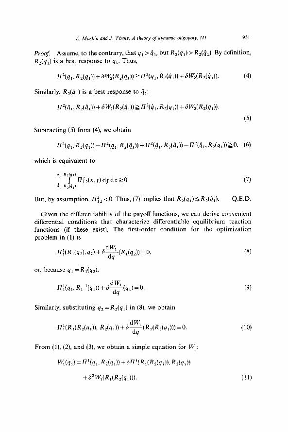
Proof Assume, the contrary, q1 > but R2(ql) R2(Q1). By definition, R2(ql) is a best response to ql. Thus,
But, by assumption, Z7:, < 0. Thus, (7) implies that R2(ql) 5 R2(gI). Q.E.D.
Given the differentiability of the payoff functions, we can derive convenient differential conditions that characterize differentiable equilibrium reaction functions (if these exist). The tirst-order condition for the optimization problem in (1) is
#(R,(q,)> q2) + 8’ T(R,(q,)) =O,
or, because q1 =Rl(q2),
W, n:(ql, R, ‘(41)) + 6 ~ dq (41)=@
(8)
(9)
Similarly, substituting q2 = R2(ql) in (8) we obtain
From (l), (2), and (3) we obtain a simple equation for WI:
(10)
(11)
952 E. Maskin and J. Tirole, A theory of dynamic oligopoly, III
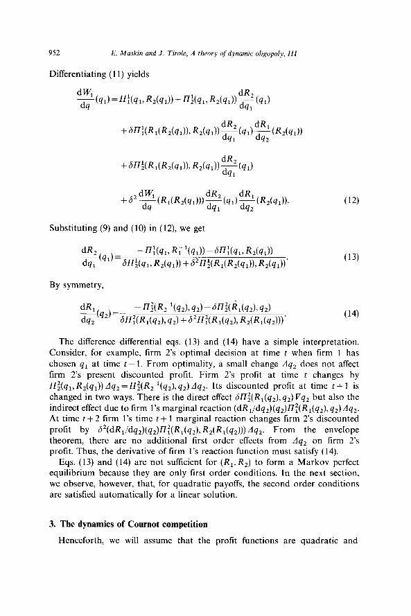
The differencedifferential eqs. (13) and (14) have a simple interpretation. Consider, for example, firm 2’s optimal decision at time t when firm 1 has chosen q1 at time t - 1. From optimality, a small change Aq, does not affect firm 2’s present discounted profit. Firm 2’s profit at time t changes by Z7:(q,, R,(q,)) Aq, =ZI$(R; ‘(q2), q2) Aq,. Its discounted profit at time t + 1 is
changed in two ways. There is the direct effect 61Z:(Rl(q,),q2) Vq2 but also the indirect effect due to firm l’s marginal reaction (dRl/dq2)(q2)17$Rl(q2), q2) Aq,.
At time t + 2 firm l’s time t + 1 marginal reaction changes firm 2’s discounted
profit by ~2(dRlldq2)(q2)~:(Rl(q2), R2(Rl(q2))) Aq2. From the envelope theorem, there are no additional first order effects from Aq, on firm 2’s profit. Thus, the derivative of firm l’s reaction function must satisfy (14).
Eqs. (13) and (14) are not sufficient for (R,,R,) to form a Markov perfect equilibrium because they are only first order conditions. In the next section, we observe, however, that, for quadratic payoffs, the second order conditions are satisfied automatically for a linear solution.
3. The dynamics of Cournot competition
Henceforth, we will assume that the profit functions are quadratic and
E. Maskin and J. Tirole, A theory of dynamic oligopoly, 111 953
symmetric. Specifically,
P=qi(d-qi-qj) where d>O. (15)
The quantity ZIi can be thought of as firm i’s profit in Cournot competition when the demand function and the production costs are linear. Then, d
represents the difference between the intercept of the demand curve and the marginal cost c.’ We note that the ‘reaction’ functions3 of the standard static Cournot model are
RTtqj) = Cd - qj)/23 i-l,2 (16)
and that the static equilibrium is given by
q”1 =q;=d/3.
Differentiating (15) and (16), we obtain partial derivatives:
l7j=d-2qi-qj (17)
and
n;= -qi. (18)
The linearity of these partial derivatives leads us to look for linear dynamic reaction functions:
(19)
where from Lemma 1, a, > 0 and bi > 0. Substituting (19) into (13) and (14) gives us the following two conditions in
But from these two equations, it is clear that b, = b,. Hence, we can drop the subscripts to obtain
62b4+26b2-2(1 +6)b+ 1 =O. (20)
20ne can work with either of two specifications of the model. In the first, quantities and price are unconstrained (i.e., can be negative) and payoffs are given by (15). In the second (more economic) specification, quantities must be non-negative and if q,+qjzd, firm i’s profit is equal to -ccq, (the price cannot be negative). The two alternatives yield the same MPE, and so we need not choose between them.
‘These are, of course, not truly reaction functions because, in a one-period model, there is no opportunity to react.
954 E. Maskin and J. Tirole, A theory of dynamic oligopoly, Ill
Eq. (20), which determines the slope of the reaction function, has two real roots:4 one in the interval (O,+) and the other in the interval (l/& l/6). As we will see below, only the former is relevant for our purposes. This root leads to dynamic reaction functions for which there is a steady-state output @= l/( 1 +b) and that are dynamically stable, i.e., starting from any produc- tion level (ql, qz), production converges over time to the steady-state (q’, 4’). The other root gives rise to a dynamically unstable path.’
From (13) (14), and (19), we have
62b3ui-62b2uj+6bui+~j=(l+6)db, i= 1,2, j#i.
Subtracting one of these equations from the other, we obtain
But as may be readily verified, the coefficient of a, -a, does not vanish in the interval (O,$, and so a, =u2. We may, therefore, drop the subscripts from the u’s to obtain
(1 +S)b
u=62b3-b2b2+bb+l d= l+b pd,6
3-6b (21)
where the second equation in (21) is obtained using (20).
Proposition 1. For any discount factor 6: (1) there exists a unique linear MPE Cgiven by (19)421)], (2) this MPE is dynamically stable; i.e., for any
history of the game, the production levels converge to steady state outputs (q’,qe), (3) each firm’s steady state output q’ is equal to the static Cournot
equilibrium output d/3 when 6 =0 [in which case, the dynamic reaction functions coincide with their static counterparts, given by (16)] and grows with the discount factor.
4This follows because the left-hand side of (20) is negative for h = l/2 and tends to infinity as h goes to either plus or minus infinity and because its second derivative is everywhere positive.
‘In our first specification (unconstrained quantities and price; see footnote 2), the two firms’ intertemporal payoffs fail to converge for this root; their instantaneous payoffs ‘chatter’ between negative and positive values that tend to - a and + m. This root can also be ruled out in our second specification (at least for discount factors that are not too small), because, starting from a point where the other firm sets q=a/h, a firm earns zero intertemporal profit, although it could make a strictly positive profit by playing the (unstable) steady-state output. By contrast, our stable root gives a piece-wise linear solution (R(q) = a - hq for 0 5 4 5 a/h, 0 for 4 2 a/h) that is an MPE over the whole positive quadrant (not only in the subspace [0,a/b12) as can easily be checked.
6 In this case where the tirms’ marginal costs dither, the slopes of the reaction functions are the same and given by (20) but the intercepts differ.
E. Maskin and .I. Tirole, A theory of dynamic oligopoly, III 955
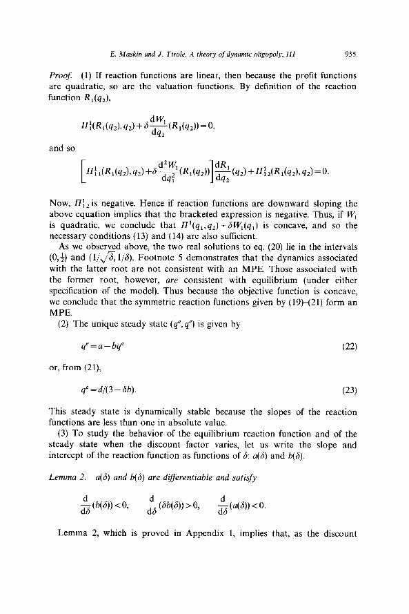
Proof: (1) If reaction functions are linear, then because the profit functions are quadratic, so are the valuation functions. By definition of the reaction
Now, II:, is negative. Hence if reaction functions are downward sloping the above equation implies that the bracketed expression is negative. Thus, if WI is quadratic, we conclude that LZ’(q,,q,) +6W,(q,) is concave, and so the necessary conditions (13) and (14) are also sufficient.
As we observed above, the two real solutions to eq. (20) lie in the intervals (O,& and (l/A l/6). Footnote 5 demonstrates that the dynamics associated
with the latter root are not consistent with an MPE. Those associated with the former root, however, are consistent with equilibrium (under either specification of the model). Thus because the objective function is concave, we conclude that the symmetric reaction functions given by (19)+21) form an MPE.
(2) The unique steady state (q’,qe) is given by
q’=a-bq” (22)
or, from (21),
qe=d/(3-6b). (23)
This steady state is dynamically stable because the slopes of the reaction functions are less than one in absolute value.
(3) To study the behavior of the equilibrium reaction function and of the steady state when the discount factor varies, let us write the slope and intercept of the reaction function as functions of 6: a(6) and b(6).
Lemma 2. a(6) and b(6) are dijjferentiable and satisfy
Lemma 2, which is proved in Appendix 1, implies that, as the discount
956 E. Maskin and J. Tirole, A theory of dynamic oligopoly, III
factor grows, the slope and the intercept of the reaction function decrease, and the steady state output increases [from eq. (23)].
When 6 =O, the firms do not care about their future payoffs; they move according to their static (Cournot) reaction functions, given by (16). This can be seen from eqs. (20) and (21): a(0) =d/2, b(0) = l/2. As 6 grows, each firm takes its opponent’s reaction more seriously; a and b decrease and q’
increases. A numerical analysis of (20), (21) and (23) shows that when 6 converges to 1, the limiting values of a, b and q’ are: a= 0.48d, b r0.30, q’r0,37d. These values are the same as those found by Cyert and de Groot when they numerically computed the perfect equilibrium solution for the no- discounting finite-horizon game and took the limit as the horizon grows (see the convergence theorem, Proposition 2, below for an explanation of this coincidence). Q.E.D.
Remark. The convergence toward the static Cournot reaction functions when 6 tends to 0 is a special case of a very general result obtained by Dana and Montrucchio (1986). They study MPE’s of the alternating move game with strategies spaces that are compact and convex subsets of Euclidean spaces and with continuous payoff functions that are concave in a player’s own action. They show that equilibrium dynamic reaction functions exist for all discount factors 6, that valuation functions are upper semicontinuous, and that equilibrium converges to the Cournot reaction functions as 6 tends to 0.’
The dynamic reaction functions for 6 in (0,l) are depicted in fig. 1. The dotted lines represent the static reaction functions R”, and R; (which correspond to S=O), and the solid lines the dynamic reaction functions R, and R,. E denotes the steady state allocation, and C the Cournot outcome. An example of a dynamic path is also provided.
That the outcome in our dynamic model is more ‘competitive’ than in the static case should not surprise us. In each period of the dynamic game, the firm about to move, say firm 1, takes two considerations into account: its short-run profit and the reaction it will induce in firm 2. Suppose that firm 2 is currently at the Cournot level. Then a slight increase in output above the Cournot level by firm 1 will have no effect (to the first order) on short-run profit. However, because reaction functions are downward-sloping, the increase will induce firm 2 to reduce its output below the Cournot level the following period, thereby increasing firm l’s long-term profit. This argument suggests that firm 1 has an incentive to choose a higher output in a dynamic rather than in a static setting because, each time it moves, it acts as a ‘Stackelberg leader’. Since this is true of firm 2 as well, the end result is output above the Cournot level (i.e., more competitive behavior) by both firms.
‘They also show that any pair of twice differentiable functions is an MPE of some game for a small enough discount factor.
E. Maskin and J. Tirole, A theory of dynamic oligopoly, III 957
This result contrasts with our findings when firms compete instead in prices. In that case, reaction functions can be upward-sloping, and thus dynamic equilibrium typically entails a less competitive outcome than its static counterpart [see Maskin and Tirole (1985)].
An increase in the discount factor means either that firms have become more patient (r has fallen) or that the reaction lag T has shrunk. A fall in the interest rate makes a firm more willing to forego current profits to induce the other firm to curtail its output. Thus, competition is enhanced. A decrease in the reaction lag T also fosters competition because it means that the period of time before the other firm reacts becomes decreasingly significant relative to the future. As T tends to 0, 6 tends to 1, and the steady-state output diverges increasingly from the Cournot output. This result implies that the relative timing of firms’ moves matters crucially, even in the limit when firms react very quickly. To see this, contrast our results with those of the simultaneous move game, where the (unique) MPE involves static Cournot outputs in every period. We conclude that the distinction between simulta- neous and alternating moves remains important even when T is very small.
4. Finite and infinite horizons
We have been unable to show that the equilibrium of Proposition 1 is the
958 E. Maskin and J. Tide, A theory of dynamic oligopoly, III
unique MPE of the infinite horizon game (it is, of course, unique within the linear class). It nonetheless possesses another attractive property, viz., it is the limit of the (unique) perfect equilibrium of the truncated finite horizon game when the horizon tends to infinity.
The finite horizon game is obtained from our infinite horizon model by truncating payoffs. In some time period, the game terminates, and all subsequent profits are zero. One computes the equilibrium of the finite horizon game by backward induction. In the last period, the firm about to move, say firm 1, plays according to its static reaction function. A period earlier, firm 2 moves knowing that the first firm will respond on its static
reaction function, etc. (see below for a more detailed description of the induction). These considerations define reaction functions that depend on the period of play and the length of the horizon (they actually depend only on the difference between these two numbers). For a given finite horizon, perfect equilibrium is readily shown to be unique. Therefore, the equilibrium reaction functions depend only on the payoff-relevant state (any game of complete information admits an MPE. Hence, if perfect equilibrium is unique, it is necessarily Markov); a firm’s action at time t depends only on
its competitor’s output at t- 1. To compute the finite horizon reaction functions analytically appears
intractable. We can demonstrate, however, that for any fixed time period, a firm’s finite horizon perfect equilibrium reaction function for that period converges to the (infinite horizon) MPE reaction function as the horizon
tends to infinity.
Proposition 2. Fix a date t. In the model with horizon v( > t), a firm’s perfect
equilibrium reaction function at date t converges uniformly to the infinite MPE reaction function given by (19)421) as V+CO.
Proof: Consider a horizon of length v. It will prove convenient in our argument to index periods counting backwards from the end. Thus. the last period is indexed 0, and the first period is u- 1. Suppose, for example, that firm 2 moves at time 0. As we already noticed, the best that it can do at time 0 is to play according to its static reaction function: R’(q) = R”(q) (where q denotes firm l’s output at time 1, and R” is the static reaction function). Consider the decision problem of lirm 1 at time 1. Its reaction R’(q) is given
by R’(q) =argmax {fll(<, q) + 6I7’(& R’(Q))}.
4 (24)
Similarly, firm 2’s optimal strategy R2(q) at time 2 satisfies
E. Maskin and J. Tirole, A theory of dynamic oligopoly, Ill 959
Thus, the reaction function R2 is determined by the succeeding two reaction functions, R’ and R”. More generally, the reaction function R’ of a lirm moving at time z is determined by R’-’ and Rre2. Specifically, let
where H’(ij, q) s $(d- q - 4). By definition, R*(q) = arg maxg H’(@, q). Thus, from the envelope theorem,
[d-24-q]+6 d-24-RT-‘(+4~(cj)] [
+d2 -Rzp2(R”(q3)~(4)]=0,
Thus, R’ is determined by R’~ 1 and Rfd2.
Although it seems impossible to derive R’ analytically, one can character- ize it by induction. In particular, Appendix 2 demonstrates that R’ is linear and has a slope between -4 and 0. Let L be the set of linear functions with slope between -3 and 0 and intercept between 0 and d. Consider the mapping m defined on L x L by
X(q) = arg max {fl’& 4) + 8n1(4 Z(G)) + d2n1(R(Z(X(q))), Z(g)). B
Note that in the definition of Z and X, we take the reaction two periods hence as given. Then, from the envelope theorem, the maximizations on the right-hand sides of these definitions are equivalent to those of the full intertemporal objective function. Note also that
(R 2k+l,R2k)=m(R2k-‘,R2k~2)~ (27)
We consider the following metric on the space L x L. Take
where R(q) = aR - bRq and I?(q) = 6, - i&q, s(q) = U, - b,q, s(q) = ii, - b”,q.
960 E. Maskin and J. Tirole, A theory of dynamic oligopoly, III
Appendix 2 shows that, for d sufficiently small, m is a contraction mapping on L x L with this metric. Thus, there exists K < 1 such that if (X, Z) = m(R, S)
and (8,Z)=m(B,!?)), then Il(X,Z)-(8,2)11rKII(R,S)-(I?,~))II. The contraction mapping property has a useful consequence [see, eg.,
Smart (1974, theorem 1.1.2)], namely, the sequence {(R2k+1,R2k)}km_0 con- verges uniformly to a fixed point (R,,R,) of m:
(Rl, R2) =m(Rl, R2) (28)
[(R,,R,) is, moreover, the unique fixed point of m in Lx L]. Given that (R,,R,) is a fixed point,
Thus, (R,,R,) is a Markov perfect equilibrium of the infinite horizon game. Because the infinite horizon linear MPE given by (19)<21) belongs to L x L,
it must therefore coincide with (R,,R,). The preceding argument applies when d is sufficiently small. But if Rf; is
the k-period equilibrium reaction function for given d and R:(q) = ai- biq,
then Rj(q) = (a/d),: - biq. Thus the same conclusion obtains for all d. Q.E.D.
5. Adjustment costs
We have formalized inertia in decision making by assuming a two period commitment to output decisions. Inertia arises because technology decisions take time, contracts with suppliers cannot readily be changed, and so forth. A shortcoming of our two-period commitment structure is that it fails to make the implicit cost of changing output sensitive to the current output level (although it does make this cost time-contingent). One would expect that often small adjustments are cheaper than large ones. In this section, we introduce output-related adjustment costs to our model. We show that our techniques for studying differentiable MPE’s can be extended to this more elaborate construct (which has a two-dimensional state space).
We assume that, if firm i moves at time t, it incurs a cost (beyond the variable cost already embodied in ZI’) depending on its current choice, qi,t, and previous output, qi,t_2. Let Ai(qi,t, qi,t_2) represent this adjustment cost,
which we assume is differentiable. Because qi,t- 2 influences firm i’s current profit at time t, the payoff-relevant state is (qj,,_l,qi,t_2). Thus, a Markov
E. Maskin and J. Tirole, A theory of dynamic oligopoly, Ill 961
strategy at time t takes the form
4i,t=Ri(qj,,~1,qi.t-2). (29)
The definition and properties of a Markov perfect equilibrium are the
same as before. To solve for such an equilibrium, one could use the valuation function approach of section 2. Instead, we will derive the difference- differential equations using marginal reasoning. Assume that firm 1 chooses ql,t at time t. A small increase above the optimal ql,* does not affect firm l’s present discounted payoff to the first order. Thus, we have
[
a& +6 ~I:(41,*~42,t+l)~4+~l(4l.t~42,t+l)~~4
h,, 1
(30)
where
(31)
(32)
As before, terms corresponding to later periods in (30) vanish due to the envelope theorem. The difference-differential equation corresponding to firm 2’s move can be written similarly.
We now consider symmetric and quadratic profit functions and adjustment costs:
ni = qi(d - qi - qj), (34)
(35)
The following proposition is proved in Appendix 3:
Proposition 3. There exist parameter values (a, b, /?), depending on (6, d, ~1) such that the dynamic reaction functions Ri(qj,,_1,qi,t_2)=a-bqj,,_ 1 +pqi,l-z form
962 E. Maskin and J. Tirole, A theory of dynamic oligopoly, Ill
a Markov perfect equilibrium of the market with adjustment costs. Furthermore, for any discount factor, 6, the steady-state output q’=a/(l + b-/I) tends to
the static Cournot output q” as the adjustment cost parameter, CI, becomes large.
Thus, as modelled, adjustment costs tend to weaken competition (remem- ber that, for a =O, b=O and the steady-state output exceeds the Cournot level). Roughly speaking, this occurs because when a firm decreases its output (a ‘cooperative’ gesture), the other firm is less tempted to take advantage of this reduction by increasing its own output if adjustment costs are high. Of course, adjustment costs will also influence future decisions, but Proposition 3 shows that these effects do not interfere with the intuitive story.
To see why high adjustment costs lead to a steady state near the Cournot outcome, suppose that the firms start at the Cournot allocation. When a firm increases its output above its Cournot level, the other firm curtails its own output. But the higher the adjustment costs, the smaller the decrease in output, and so the smaller the gain to the aggressive firm. As adjustment costs grow, therefore, the short-run loss associated with the increase in
output becomes more and more important. Of course, the modelling of adjustment costs here, although an improve-
ment over previous sections, remains crude. There are, no doubt, more subtle forms of inertia that do not fall conveniently into our time-and-output- contingent framework.
6. Endogenous timing
As we suggested in ihe introduction, the alternating moves feature of our model is a property that ought to be derived from more primitive assump- tions rather than simply imposed. Indeed, in our earlier work on quantity competition with large fixed costs [Maskin and Tirole (1982)] and price competition [Maskin and Tirole (1985)], we proposed two rather different ways of ‘endogenizing’ the relative timing of firms’ moves. In both cases, however (and in both the quantity and price settings) firms end up in equilibrium behaving exactly as in the fixed timing framework, i.e., alternating.
In this section, we briefly review the two endogenous timing models. We observe, however, that, in contrast with our previous results, they provide conflicting answers when applied to the Cournot setting. Although one gives rise to an equilibrium formally identical to that explored above, the other predicts that, in the steady state, firms move simultaneously. This conflict suggests that a more detailed study of the micro-foundations of timing in firms’ decision-making is called for, an ambitious task that will have to be deferred to the future.
E. Maskin and J. Tirole, A theory of dynamic oligopoly, III 963
Probably the easiest way to obtain alternating moves endogenously is to posit a continuous time model where commitments are of random length. Suppose that, as before, when a firm chooses a quantity level, it remains committed to that level for some period of time, but now assume that the period is uncertain. The simplest such hypothesis is that the probability that a commitment will lapse during a (short) interval At is proportional to the interval’s length. That is, commitment terminations occur according to a Poisson process [for a more detailed presentation of this model, see Maskin and Tirole (1982)]. In this model, the mean length of time before some firm moves corresponds precisely to a single period in the fixed timing framework. Because, moreover, the probability that firms’ commitments will lapse simultaneously is zero, equilibrium retains the feature that firms move alternately.
Turning to a somewhat different model, we revert to discrete time but now abandon the assumption that firm 1 can move only in odd-numbered periods and firm 2 only in the even-numbered ones. Instead we suppose that a firm can, in principle, move in any period but, once it does so, remains committed for two periods. Thus in any period where a firm is not already committed, it can choose a quantity level. Alternatively, it can refrain from moving at all, that is, it can produce nothing (in which case, it is free to move at any future date).
The considerations affecting the payoff of a firm about to move are (i) whether the other lirm is currently committed to a quantity level, and (ii) if so, which quantity. Thus, Markov strategies (on which we continue to concentrate) now depend on a two-dimensional payoff-relevant state.
Despite the freedom firms have in this model to vary their relative timing, one can show that, at least for discount factors near 1, any MPE has the
properties that (i) starting from any point, a steady state is reached with probability one, and (ii) a steady state involves firms choosing Cournot quantities and moving simultaneously.
We will omit the formal demonstration of this result, but the intuition is not hard to provide. We have seen that when firms move alternatingly, they have a tendency to produce higher quantities leading to lower profits than were they to move simultaneously. Thus, the firms have a joint incentive to be in a simultaneous rather than alternating ‘mode’. This, of course, is a cooperative, rather than individual, consideration. Just because firms would be better off moving simultaneously does not mean that an individual firm will make the first move to bring this about. It may well prefer that the other firm move first, and so, given the other firm’s reciprocal attitude, firms may get ‘stuck’ moving alternatingly. When there is little discounting, however, the ultimate gain from moving simultaneously swamps the individual cost of engineering the transition from the alternating mode. Thus simultaneity ultimately prevails.
964
Appendix 1
E. Maskin and J. Tide, A theory of dynamic oligopoly, I11
Proof of Lemma 2 (d(Sb)/dS > 0, db/dS < 0, da/dS < 0). Totally (20), we obtain
Eqs. (A.1 l)<A.13) determine the equilibrium values of a, b and fi. As the adjustment parameter CI goes to infinity, we obtain, from (A.11))
(A.13), the following limiting values of a, b, B and the steady-state output qe:
uzd(l+@/c(, bz(l+6)/a,
pz.-2(1+6)/a, q’zdd/3 =qs (the static Cournot quantity).
‘Actually, we have shown only that m contracts points that are sufficiently close together. But the distance between any two points can be subdivided into such small intervals, and so m consequently contracts all pairs of points.
References
Cournot, A., 1838, Recherches sur les principes mathematiques de la theori des Richesses (Hachette, Paris).
968 E. Maskin and J. Tirole, A theory of dynamic oligopoly, III
Cyert, R. and M. de Groot, 1970, Multiperiod decision models with alternating choice as the solution to the duopoly problem, Quarterly Journal of Economics 84, 410-429.
Dana, R.A. and L. Montrucchio, 1986, Dynamic complextty in duopoly games, Journal of Economic Theory, forthcoming.
Friedman, J., 1977, Oligopoly and the theory of games (North-Holland, Amsterdam). Kreps and Scheinkman, 1983, Quantity precommitment and Bertrand competition yield
Cournot outcomes, Bell Journal of Economics 14, 326337. Maskin, E. and J. Tirole, 1982, A theory of dynamic oligopoly, I: Overview and quantity
competition with large fixed costs, Econometrica, forthcoming. Maskin, E. and J. Tirole, 1985, A theory of dynamic oligopoly, II: Price competition,
Econometrica, forthcoming. Smart, D.R., 1974, Fixed point theorems (Cambridge University Press, New York).


![Building brand awareness in dynamic oligopoly marketsheuristic.kaist.ac.kr/cylee/xpolicy/termproject/08/[4]brand awareness.… · Oligopoly market Characteristic of Oligopoly market](https://static.documents.pub/doc/80x56/5ebda2b9fa9af9629303f297/building-brand-awareness-in-dynamic-oligopoly-4brand-awareness-oligopoly-market.jpg)


