A Theory of Income Smoothing When

Insiders Know More Than Outsiders∗

Viral Acharya

NYU-Stern, CEPR and NBER

Bart M. Lambrecht

Lancaster University Management School

7 November 2011

Abstract

We consider a setting in which insiders have information about income that

outside shareholders do not, but property rights ensure that outside shareholders

can enforce a fair payout. To avoid intervention, insiders report income consistent

with outsiders’ expectations based on publicly available information rather than

true income, resulting in an observed income and payout process that adjust

partially and over time towards a target. Insiders under-invest in production

and effort so as not to unduly raise outsiders’ expectations about future income,

a problem that is more severe the smaller is the inside ownership and results in an

“outside equity Laffer curve”. A disclosure environment with adequate quality

of independent auditing mitigates the problem, implying that accounting quality

can enhance investments, size of public stock markets and economic growth.

J.E.L.: G32, G35, M41, M42, O43, D82, D92

Keywords: income smoothing, payout policy, asymmetric information, under-

investment, accounting quality, measurement error, finance and growth.

∗We are grateful to Phil Brown, Stew Myers, John O’Hanlon, Ken Peasnell, Joshua Ronen, Stephen

Ryan, Lakshmanan Shivakumar and Steve Young for insightful discussions. Comments can be sent

to Viral Acharya (vacharya@stern.nyu.edu) or Bart Lambrecht (b.lambrecht@lancaster.ac.uk).

A Theory of Income Smoothing When Insiders Know More Than

Outsiders

Abstract

We consider a setting in which insiders have information about income that outside

shareholders do not, but property rights ensure that outside shareholders can enforce

a fair payout. Insiders report income consistent with outsiders’ expectations based on

publicly available information rather than true income, resulting in an observed in-

come and payout process that adjust partially and over time towards a target. Insiders

under-invest in production and effort so as not to unduly raise outsiders’ expectations

about future income, a problem that is more severe the smaller is the inside ownership

and results in an “outside equity Laffer curve”. A disclosure environment with ade-

quate quality of independent auditing mitigates the problem, implying that accounting

quality can enhance investments, size of public stock markets and economic growth.

J.E.L.: G32, G35, M41, M42, O43, D82, D92

Keywords: income smoothing, payout policy, asymmetric information, under-investment,

accounting quality, measurement error, finance and growth.

Introduction

A fundamental property right conferred upon stockholders of a firm is that they are

entitled to their fair share of the firm’s (distributable) net income. Since stock owner-

ship is verifiable, this right is relatively easy to enforce provided that everyone agrees

on what the income is. In a world of complete information, determining net income

should be a relatively simple matter because it is clear to everyone to see how much

money is left on the table after all senior claimants (creditors, managers, employees,

taxman, ...) have been paid. Matters become more tricky in a world of asymmetric

information where inside shareholders have full information, and outside shareholders

have partial information.

How is income reported and payout determined if asymmetric information is a fact

of life? What are the effects of information asymmetry on insiders’ production decision

or incentives to put in effort? How does asymmetric information affect the time-series

properties of reported income and payout? How does inside ownership affect income

and operating efficiency? These are some of the questions we try to address in this

paper.

We consider an all-equity financed firm that pays out each period all realized income.

In our model outsiders can extract their share of income from the firm by a threat

of collective action against insiders.1 While under symmetric information outsiders

know exactly what they are due, under asymmetric information outsiders refrain from

intervention for as long as the reported income (and corresponding payout) meets

their expectations. Outsiders (supported by analysts) form their expectations about

income on the basis of the information available to them. Outsiders’ income estimate

is unbiased and “best” based on the information they have available, and it is therefore

rational for them to require a payout that is consistent with their expectations.2 Hence,

1If collective action is costly (as in Myers (2000), Jin and Myers (2006), Lambrecht and Myers

(2007, 2008), Acharya, Myers and Rajan (2011), among others) then this gives insiders scope to

extract rents, which erodes outsiders’ stake in the firm’s income and the value of the outside equity. A

strictly positive cost of intervention is not central to our paper. We rule out, however, the possibility

that property rights are void and outsiders cannot extract any income from the firm as this would

completely undermine the firm’s capability to raise outside equity in the first place.2Policies where insiders pay out according to realized income would be “fragile” for insiders. For

instance, if realized payouts are repeatedly below outsiders’ estimates, then outsiders may believe they

1

when the strength of property rights and pressure by outside investors keeps insiders to

the straight and narrow, the equilibrium payout will be smooth compared to realized

income as it is based on outsiders’ expectation. Insiders absorb short term variation

in income and, if necessary, have to “find the money” to keep outside investors at bay.

So far smoothing is fairly harmless in that it merely irons out variation in reported

income. We call it “financial smoothing” because it merely alters the time pattern of

reported income (through borrowing and savings) without changing the firm’s under-

lying cash-flows as determined by insiders’ production and effort decisions. Insiders

may, however, also engage in “real smoothing” by manipulating production and effort

decisions in an attempt to “manage” outsiders’ expectations. In particular, if outsiders

cannot observe value-relevant variables (such as marginal costs) directly but have to

rely on an incomplete set of observable proxies (such as output or sales) in order to

infer income indirectly, then insiders may have an incentive to distort the observable

proxy variables in order to lower outsiders’ expectations about current and future in-

come. The logic of this results is as follows. Suppose that outsiders can observe realized

sales (revenues) but not costs. In particular, the firm’s marginal cost is a stochastic

latent variable. While outsiders do not know the realization of the marginal cost, the

parameters that drive the marginal cost process are common knowledge. As before

outsiders expect their fair share of income. Insiders know that outsiders associate a

higher sales level with lower marginal costs. Therefore, upon observing higher sales,

outsiders expect income to be higher and want higher payout. In an attempt to “man-

age” outsiders’ expectations , insiders underproduce and engage in “signal-jamming”.

Insiders cut output up to the point where the cost in terms of reducing expected income

equals the benefit of lowering outsiders’ payout expectations.

In contrast, in an environment of symmetric information where payout to outsiders

is a function of actual income (i.e. cash-flows), insiders determine the firm’s output

(and therefore sales) level at the first-best by setting marginal costs equal to marginal

revenues.3

Now, though insiders underproduce in order to “fool” outsiders, in equilibrium they

are being taken for a ride by insiders and intervene.3In effect, insiders have an incentive to maximize total firm value and to put in the optimal effort

level if they get (i) a constant fraction of the firm’s actual (i.e. realized) income and, (ii) a perfectly

competitive remuneration (taken upfront out of gross revenues) for their cost of effort.

2

are not successful in their attempt because insiders anticipate what is going on and can

still infer from sales the value of the latent cost variable if that is the only unobservable

(i.e., assuming there are no other unknowns to outsiders). Reported income therefore

coincides with actual income. Nevertheless, indirect inference of costs through sales

distorts insiders’ actions and traps them into behaving myopically.

Next, assume that observed sales are affected each period by an additive, indepen-

dently and identically distributed, noise term, the realization of which is unknown to

insiders at the time when they set the output level. The noise term could, for instance,

reflect measurement error. Such noise causes sales to become an imperfect (noisy) mea-

sure of the latent marginal cost variable. As a result outsiders can no longer infer the

exact realization of actual income because they do not know whether a change in sales

is due to measurement error or a change in the latent cost variable. However, since

measurement errors are transitory and shocks to costs persistent, the underlying source

of change gradually becomes clear over time. Therefore, outsiders calculate their best

estimate of income on the basis of not only current sales but also past sales. Indeed,

while the current sales figure could be unduly influenced by measurement error, an

estimate based on the full sales history will smooth out the effect of this random noise

term.

Formally, outsiders’ income estimate is the solution to a filtering problem. We

adopt the Kalman filter because for our linear model with Gaussian disturbances the

Kalman filter gives an unbiased, minimum variance and consistent estimate of actual

(i.e. realized) income.4 While at any given time the Kalman filter is an inexact

estimate of actual income, the measure is right on average and optimal among all

possible estimators.

Then, in a rational expectations equilibrium outsiders calculate their expectation of

actual income on the basis of realized sales and of what they believe insiders’ optimal

output and effort policy to be. Conversely, insiders determine each period their optimal

effort and output policy given outsiders’ beliefs. In equilibrium insiders’ actions are

consistent with outsiders’ beliefs and outsiders’ expectations are unbiased conditional

on the information available. Each period outsiders receive a payout that equals their

share of what they expect income to be. Insiders also get a payout but they have to soak

4 For an early forecasting application of Kalman filter in the context of earnings numbers, see

Lieber, Melnick, and Ronen (1983), who use the filter to deal with transitory noise in earnings.

3

up any under (over) payment to outsiders as some kind of discretionary remuneration

(charge): if actual income is higher (lower) than outsiders’ estimate then insiders cash

in (make up for) the difference in outsiders’ payout.

We obtain “income smoothing” because insiders report an income figure that corre-

sponds to outsiders’ beliefs (since there is no credible way of conveying actual income).

Consequently, reported income and payout are smooth compared to actual income not

because insiders want to smooth income, but because insiders have to meet outsiders’

expectations to avoid intervention.5

In addition to smoothing in a static sense, i.e., that payout is linked not to actual

income, but to income as expected by outsiders, smoothing also happens in an inter-

temporal sense and it further distorts insiders’ output and effort decision. The efficient

output and effort level should be determined only by the contemporaneous level of the

latent marginal cost variable. However, the current effort and output decision not

only affect current sales levels but also outsiders’ expectations of current and all future

income. This exacerbates the previously discussed negative externality for insiders be-

cause bumping up sales now means the outsiders will expect higher income and payout

not only now but also in future. Even though the spillover effect of a one-off increase

in sales on outsiders’ future expectations wears off over time, it still causes insiders to

underproduce even more and to put in even lower effort compared to what is first best.

We stress that intertemporal smoothing in our model does not result from risk

aversion because all agents are risk neutral. If insiders’ utility were a concave function

of reported income then this alone could be sufficient to generate smoothing in reported

income. Managerial or insider risk aversion is a pervasive feature and key driver in

existing papers on income smoothing (see related literature in section 5). There is,

however, direct support for our model in the survey-based findings of Graham, Harvey,

and Rajgopal (2005): (i) insiders (managers) always try to meet outsiders’ earnings

per share (EPS) expectations at all costs to avoid serious repercussions; and, (ii) many

managers under-invest to smooth earnings and therefore engage in real smoothing. The

5This does not mean that we never have income or “earnings” surprises. If realized sales at time t

are higher (lower) than what outsiders expected based on the information available at time t− 1 then

we still have a positive (negative) earnings surprise. However, once the sales at time t are observed,

outsiders and analysts know exactly what net income figure they expect to be released by insiders. In

this sense the reported income figure is always consistent with the latest sales figure.

4

first is one of the key premises of the model and the second is a key implication of the

model.

Our theory of intertemporal income smoothing yields rich, testable implications

on the time-series properties of reported income and payout to outsiders. First, “re-

ported income” is smooth compared to “actual income” because the former is based

on outsiders’ expectations whereas the latter corresponds to actual cash flow realiza-

tions. Second, reported income follows inter-temporally a target adjustment model.

The “income target” is a linear, increasing function of sales, so that when there is a

shock to sales (and therefore to the income target), reported income adjusts towards

the new target, but adjustment is partial and distributed over time because outsiders

only gradually learn whether a shock to sales is due to measurement error or due to

a fundamental shift in the firm’s cost structure. Third, the current level of reported

income can be expressed as a distributed lag model of current and past sales, where

the weights on sales decline as we move further in the past. Since payout to out-

siders is a fraction of reported income, it follows that also payout can be expressed as

a distributed lag model of sales. Equivalently, current payout can be expressed as a

target adjustment model where current payout depends on current sales and previous

period’s payout, which is similar to the Lintner (1956) dividend model.6 Fourth, the

total amount of smoothing can be broken up in two components: “real” smoothing

and “financial” smoothing. While the latter does not alter the underlying cash flows,

the former results in under-investment and implies that the output level (and therefore

sales) becomes less sensitive to variation in the latent cost variable.7

Importantly, smoothing increases with the degree of information asymmetry be-

tween insiders and investors. Holding constant the degree of information asymmetry,

smoothing and underproduction in particular also increase with the outside sharehold-

ers’ ownership stake. Conversely, a higher level of inside ownership also leads to less

real smoothing. Indeed, the under-investment problem disappears as insiders move

6A difference is that in the Lintner model target payout is linked to contemporaneous net income

and not contemporaneous sales. This difference follows from the fact that sales (and not income) is

the observable “anchor” variable in our model.7We do not model how real and financial smoothing are actually implemented. The interested

reader is referred to the book by Ronen and Sadan (1981) in which the various possible smoothing

mechanisms are discussed and illustrated in great detail.

5

towards 100% ownership.8 We show that these effects lead to an “outside equity Laffer

curve”: the value of the total outside equity is an inverted U-shaped function of out-

siders’ ownership stake. The analogy with the taxation literature is straightforward:

ex post outsiders’ ownership stake acts like a proportional tax on distributable income

and undermines insiders’ incentives to produce and put in effort.

This final result suggests that low inside ownership could have detrimental conse-

quences for the firm. We argue then that since outside equity may be crucial for the

development and expansion of owner-managed firms, our results offer a rationale for

imposing disclosure requirements on public companies and for improving accounting

and auditing quality. We show that, all else equal, introducing independent accounting

information, such as an unbiased but imprecise income estimate, improves economic

efficiency, increases the outside equity value, and acts as a substitute for a higher inside

ownership stake. The implication is that accounting quality, investments, size of pub-

lic stock markets, and economic growth are all positively correlated in our model, and

as empirically found in empirical literature on finance and growth (King and Levine,

1993, Rajan and Zingales, 1998, among others).

The rest of the paper is organized as follows. Section 1 presents the benchmark

case with symmetric information between outsiders and insiders. Section 2 analyzes

the asymmetric information model. Section 3 discusses the robustness and extensions

of the model, in particular, the insiders’ participation constraint and the value of

audited disclosure. Section 4 presents additional empirical implications. Section 5

briefly relates our paper to existing literature. Section 6 concludes. Proofs are in the

appendix.

8Intuitively, the smaller the insiders’ stake, the smaller is the group of insiders that has to soak up

income shocks for a larger group of outsiders. Any variation in sales feeds into outsiders’ expectations

and is “levered” up to the extent that insiders own a smaller stake. This creates an incentive for

insiders to underproduce and to make output (and therefore sales) less sensitive to changes in the

latent cost variable. In the extreme case where insiders have no stake left in the firm they produce

little or nothing, irrespective of the marginal cost level.

6

1 Symmetric information case

Consider a firm with access to a productive technology. The output from the technol-

ogy is sold at a fixed unit price, but its scale can be varied. Marginal costs of production

follow an AR(1) process with a drift that depends on the effort exercised by the tech-

nology operators. Each period marginal costs are revealed before the output scale is

chosen. A part of the firm is owned by risk-neutral shareholders (outsiders) and the

rest by risk-neutral insiders who also act as the technology operators. To start with,

we focus on the first-best scenario in which there is congruence of objectives between

outsiders and insiders, and information about marginal costs is known symmetrically

to both outsiders and insiders.

Formally, we consider a firm with the following income function:

πt = qt −q2t

2xt− 1

2ce2t (1)

where xt = Axt−1 + B et + wt−1 with wt−1 ∼ N(0, Q) , (2)

et and qt denote the chosen effort and output level. The (inverse) marginal production

cost variable xt follows an AR(1) process with auto-regressive coefficient A ∈ [0, 1) (so

that the effect of current effort on future values of x declines over time), a drift Bet,

and an i.i.d. noise term wt−1. The term ce2t/2 represents the cost of effort expressed

in monetary terms. Effort increases the value for xt, which in turn lowers the firm’s

marginal cost of production. Effort therefore increases the efficiency of the firm’s

production process. et and qt are implemented after the realization of wt−1 is observed.

All shareholders are risk-neutral, can borrow and save at the risk free rate, and

have a discount factor β ∈ (0, 1). The value of the firm is given by the present value

of discounted income:

Vt = maxet+j , qt+j ,j=0...∞

Et[∞∑j=0

βjπt+j] = maxqt+j ,j=0...∞

Et

[∞∑j=0

βj(qt+j −

q2t+j

2xt+j− 1

2ce2t+j

)](3)

Then, the first-best policies that maximize firm value are as follows.

7

Proposition 1 The first-best production policy and effort level are respectively

qot = xt , (4)

eot =B

2c(1− βA)≡ eo . (5)

The firm’s actual (i.e. realized) income and total payout under the first-best policy are

given by:

πot =xt2− 1

2ceo2 . (6)

The proposition shows that the first-best effort is constant over time and increasing

in the autoregressive coefficient A, because with non-zero autocorrelation (A > 0) the

effort level et not only affects the contemporaneous level of xt, but also all future levels

xt+i.

The first-best output level qot equals xt. Recall that a higher value for xt implies

lower marginal costs. Therefore, the output level rises with xt. As xt goes to zero,

marginal costs spiral out of control and the first-best output quantity goes to zero. Since

the shocks that drive xt are normally distributed, marginal costs could theoretically

become negative. The solution in proposition 1 no longer makes sense for negative

xt because marginal costs can, of course, not be negative. The likelihood of negative

values for xt arising is, however, negligible small if the stationary unconditional mean

of xt (given by Be1−A) is sufficiently large relative to the unconditional variance of xt

(given by Q1−A2 ). We assume this condition to be satisfied so that we can safely ignore

the occurrence of negative costs.9

Finally, note that there is a mapping from the cost variable (xt) to the output

level (qt) and the actual income level (πt). This is important for section 2 where xt is

unobservable to outside shareholders and has to be inferred from an observable proxy.

9To rule out negative values for xt altogether one could assume that xt is log-normally distributed.

This would, however, make the Bayesian updating process deployed in next section completely in-

tractable. We will therefore stick to the normal distribution throughout this paper. The normality

assumption is standard in the information economics literature. For example, Kyle (1985) and the

large number of papers that originated from this paper all assume for sake of tractability that asset

prices are normally distributed.

8

1.1 Inside and outside shareholders

So far we have assumed that all shareholders can be treated as a homogenous group

that controls the firm. We now relax this assumption by introducing inside and outside

shareholders who, respectively, own a fraction (1 − ϕ) and ϕ of the shares, ϕ ∈ [0, 1].

For example, insiders (managers and even board members involved in firm’s operating

decisions) typically own the majority of shares of private firms (ϕ < 0.5), whereas for

public firms it is more common that outsiders own the majority of shares (ϕ > 0.5).

Insiders set production policy (qt) and exert effort (et). We assume that the market

for insiders is competitive with their reservation wages normalized to zero, so that

insiders get a monetary compensation that equals their total cost of effort (i.e., ce2t/2).

Under symmetric information outsiders can infer from xt (or qt) exactly how much

effort insiders exert. Outsiders can therefore pay the competitive remuneration for

the exerted effort. In our model partial ownership does not by itself distort insiders’

effort because the efficient outcome is achieved under symmetric information. Paying

a competitive wage for effort exerted allows us to abstract from compensation issues

and to focus purely on the conflict between inside and outside shareholders that results

from asymmetric information.10

Analogous to Fluck (1998), Myers (2000), Jin and Myers (2006), Lambrecht and

Myers (2007, 2008, 2011), and Acharya, Myers and Rajan (2011), we assume that

insiders operate subject to a threat of collective action. Outsiders’ payoff from collective

action is given by ϕαVt where α (∈ [0, 1]) reflects the degree of investor protection.

To avoid collective action, insiders pay out each period a dividend dt that leaves

outsiders indifferent between intervening and leaving insiders unchallenged for another

period. If St denotes the value of the outside equity then dt is defined by:11

St = dt + βαϕEt[Vt+1] = αϕVt (7)

⇐⇒ dt + βαϕEt[Vt+1] = αϕπt + αϕβEt[Vt+1] ⇐⇒ dt = αϕπt (8)

10Graham, Harvey, and Rajgopal (2005) report that CFOs view compensation motivation as a

second-order factor, at best, for smoothing earnings.11It is not strictly necessary that all income is paid out each period. For example, if reported

income earns the risk-free rate of return within the firm (e.g. through a high yield cash account) and

is protected from expropriation by insiders, then outsiders do not require income to be paid out (see

Lambrecht and Myers (2011) for a model where the firm borrows and saves at the safe rate).

9

Equation (7) can be interpreted as a capital market constraint that requires insiders

to provide an adequate return to outside investors. Graham et al. (2005) provide

convincing evidence of the importance of capital market pressures and how they induce

managers to meet earnings targets at all costs.12

ϕ denotes outsiders’ “nominal” ownership stake. Scaling the nominal ownership

stake by the degree of investor protection α gives outsiders’ “real” ownership state

θ ≡ ϕα. It follows that the payouts to outsiders (dt) and insiders (rt) are respectively

given by θπt and (1 − θ)πt. Income (πt) is calculated net of insiders’ compensation

for effort exerted, and is shared between insiders and outsiders according to their real

ownership stake.13 The following corollary results at once.

Corollary 1 If insiders are paid a competitive wage for their efforts and all sharehold-

ers have symmetric information then insiders adopt the first-best production and effort

levels, and payout to outsiders (insiders) equals a fraction θ (1− θ) of realized income

πt.

2 Asymmetric information

We now add two new ingredients to the model. First, we introduce asymmetric infor-

mation regarding the actual realizations of the stochastic variable xt by assuming that

these are only observed by insiders. All model parameters remain common knowledge,

however. Outsiders also have an unbiased estimate x̂0 of the initial value x0.14

Second, outsiders observe the output level qt with some measurement error. Instead

of observing qt, insiders observe st ≡ qt + εt where εt is an i.i.d. normally distributed

noise term with zero mean and variance R (i.e. εt ∼ N(0, R)). The measurement

12As one surveyed manager put it:“I miss the target, I’m out of a job.” The perception of outside

investors is such that if insiders cannot “find the money” to hit the earnings target then the firm is

in serious trouble.13The amount of effort exerted can be inferred from xt or qt.14x̂0 is revealed to outside investors when the firm is set up at time zero. See section 3.3 for further

details.

10

error is uncorrelated with the marginal cost variable xt (i.e. E(wkεl) = 0 for all k

and l). In what follows we refer to st as the firm’s “sales” as perceived by outsiders,

i.e. outsiders perceive the firm’s revenues to be st, whereas in reality they are qt.15

Outsiders are aware that sales are an imperfect proxy for economic output and they

know the distribution from which εt is drawn. Importantly, insiders implement effort

(et) and output (qt) after the realization of xt but before the realization of εt is known.

Since εt is value-irrelevant noise, the firm’s actual income is still given by πt = qt −q2t2xt− 1

2ce2t . However, as qt, xt and et are unobservable outsiders have to estimate

income on the basis of noisy sales figures. Therefore measurement errors can lead to

misvaluation in the firm’s stock price.

We know from previous section that there is a mapping from the latent variable xt

to both qt and πt. The presence of the noise term εt obscures, however, this link and

makes it impossible for outsiders exactly to infer xt and πt from sales. (Recall that

insiders know xt but not εt when setting output qt and effort et.)

Assuming that insiders cannot trade in the firm’s stock and that the information

asymmetry cannot be mitigated through monitoring or some other mechanism (we

return to this in section 3.2), the best outsiders can do is to calculate a probability

distribution of income, πt, on the basis of all information available to them. This

information set It is given by the full history of current and past sales prices, i.e.,

It ≡ {st , st−1 , st−2 ...}. In particular, we show that on the basis of the initial estimate

x̂0 and the sales history, It, outsiders can infer a probability distribution for the latent

marginal cost variable xt, which in turn maps into a probability distribution for income

πt.

Formally, the outsiders obtain an estimator x̂t for xt using a Kalman filter. The

estimator x̂t depends in general not only on the latest sales figure st but on the entire

available history It of sales. However, since past sales figures become “stale” with time

and therefore less reliable to infer the current level of xt, the Kalman filter resolves

the problem by calculating a weighted average of sales where more recent sales carry

a higher weight. The Kalman estimate x̂t is unbiased (see Chui and Chen (1991) page

40): x̂t = E[xt|It] ≡ ES,t[xt] for all t, where the subscript S in ES,t[xt] emphasizes

15For further details on the sources and properties of measurement errors we refer to the extensive

literature on income measurement in economics, accounting and statistics (see Beaver (1979), Demski

and Sappington (1990) and Moore, Stinson, and Welniak (2000), among others).

11

(outside) shareholders’ expectation at time t of xt based on the information set It. The

Kalman filter is also optimal (“best”) in the sense that it minimizes the mean square

error (see Gelb (1974)).16 We focus on the steady state or “limiting” Kalman filter

which results if the history of sales It is sufficiently long.17 The steady-state Kalman

filter allows us to analyze the long-run behavior of reported income and payout.

One might think that the amount of information to keep track of becomes unman-

ageable as the sales history becomes longer. Fortunately, this is not the case because

the Kalman filter works recursively and only requires previous period’s best estimate

x̂t−1 and current sales st to calculate a new estimate x̂t. The past history of sales is

therefore encapsulated in previous period’s estimate of the latent variable. The new

best estimate x̂t is a weighted average of x̂t−1 and st. The most weight is given to the

number that carries the least uncertainty (similar to Bayesian updating). x̂t−1 is, in

turn, a weighted average of st−1 and x̂t−2. This recursive algorithm works all the way

back to the initial time t = 0, at which point we need the initial estimate x̂0 for x0 to

start the algorithm.

We can show that with asymmetric information actual income is still linear in

xt under the insiders’ optimal production policy. Hence, using their best, unbiased

estimate x̂t, outsiders can calculate the best, unbiased estimate π̂t of the firm’s income

(i.e., π̂t = ES,t[πt]). It is rational for outside shareholders to demand a payout dt

that equals dt = θES,t(πt) where ES,t(πt) ≡ E [πt|st, st−1, st−2, ...]. Indeed, the capital

market constraint requires that dt satisfies the following constraint:

St = dt + βϕαES,t[Vt+1] = ϕαES,t[Vt]

⇐⇒ dt + βϕαES,t[Vt+1] = ϕαES,t[πt] + ϕαβES,t[Vt+1] ⇐⇒ dt = θES,t[πt]

In other words, outsiders want their share of the income they believe has been realized

according to all information available to them.

While insiders cannot manage outsiders’ expectations through words (which are not

credible) they can do so through their actions. Managers can influence observable sales

16If the disturbances (εt and wt) and the initial state (x0) are normally distributed then the Kalman

filter is unbiased. When the normality assumption is dropped unbiasedness may no longer hold, but

the Kalman filter still minimizes the mean square error within the class of all linear estimators.17Under mild conditions (see appendix) the Kalman filter converges to its steady state. Convergence

is of geometric order and therefore fast.

12

(st) by their effort (et) and chosen output level (qt). For example, a lower marginal cost

(as reflected by a higher xt) gives managers an incentive to raise output, which in turn

leads, on average, to higher sales. However, this information conveying mechanism is

partially obscured by the noise term εt. As a result, it is not optimal for outsiders to

base their expectations about πt merely on st. Instead, a more accurate estimate can

be obtained by using a Kalman filter that calculates πt on the basis of the firm’s sales

history, It.

Insiders’ optimization problem can now be formulated as follows:

Mt = maxqt+j ,et+j ;j=0..∞

Et

[∞∑j=0

βj (π(qt+j, et+j) − θES,t+j [π (qt+j, et+j)])

](9)

where π(qt+j, et+j) ≡ qt+j − 12

q2t+j

xt+j− 1

2ce2t+j. Solving this problem gives the following

proposition:

Proposition 2 The insiders’ optimal production plan and effort level are given by:

qt = H xt = Hqot and et =H2B

2c(1− βA)= H2 eo ≡ e for all t (10)

Payout to outside shareholders equals a fraction θ of reported income: dt = θπ̂t where

π̂t =

(H − H2

2

)x̂t −

1

2ce2 , (11)

and where x̂t = (Ax̂t−1 + Bet)λ + K st (12)

=λBe

1− λA+ K

∞∑j=0

(λA)jst−j . (13)

H is the positive root to the equation:

f(H) ≡ H2K(θ

2− βA) +H [βA(1 +K)− 1− θK] + 1− βA = 0 (14)

with K ≡ HPH2P+R

, λ ≡ (1−KH) and P is the positive root of the equation:

P = A2P − A2H2P 2

H2P +R+ Q . (15)

The error of outsiders’ income estimate (πt − π̂t) is normally distributed with mean

zero (i.e., ES,t[πt − π̂t] = 0) and variance σ̂2 ≡ ES,t[(πt − π̂t)2] =

(H − H2

2

)2

P .

13

The proposition describes a rational expectations equilibrium where outsiders infer an

estimate π̂t = ES,t[πt|It] for current income πt on the basis of It, the history of current

and past sales. Insiders take this expectation building mechanism as given. When

setting qt and et insiders know their choice will affect sales and therefore outsiders’

expectations of current and future income. A rational expectations equilibrium is

obtained by ensuring that insiders’ optimal production and effort policy is consistent

each period with the way outsiders form their expectations about income. In other

words, outsiders’ expectations are rational given insiders’ effort and output policy, and

insiders’ effort and output policy are optimal given outsiders’ expectations.

Since st = qt + εt the proposition implies that sales are an imperfect (noisy)

measure of the latent variable xt, as is clear from the following “measurement equation”:

st = H xt + εt with εt ∼ N(0, R) (16)

Outsiders know the variance R of the noise, εt, and the parameters A, B and Q of the

“state equation”:

xt = Axt−1 + B et + wt−1 with wt ∼ N(0, Q) for all t (17)

Using the Kalman filter (see appendix), the measurement equation can be combined

with the state equation to make inferences about xt on the basis of current and past

observations of st. This allows outsiders to form an estimate of actual income πt.

The proposition is formulated in terms of the steady state or “limiting” Kalman

filter. One can show (see appendix) that the steady state estimator for xt is given by:

x̂t ≡ ESt[xt] = (Ax̂t−1 +B e)λ + Kst (18)

where λ and K are as defined in the proposition. K is called the “Kalman gain” and

it plays a crucial role in the updating process. In the absence of measurement errors

xt can be inferred with perfect precision because x̂t = Kst = st/H if R = 0.

Substituting x̂t−1 in (18) by its estimate, one obtains after repeated substitution:

x̂t = Beλ[1 + λA+ λ2A2 + λ3A3 + ...

]+ K

[st + λAst−1 + λ2A2st−2 + λ3A3st−3 + ...

]=

Beλ

1− λA+ K

∞∑j=0

λjAjst−j . (19)

Thus, outsiders’ estimate of current actual income is not only determined by their

observation of current sales but also by the whole history of past sales. The weight

14

KλjAj that is put on past sales levels declines, however, with time because λA < 1.

The important implication is that the insiders’ optimization problem is no longer static

in nature but inter-temporal and dynamic. Indeed, the current production decision not

only affects insiders’ current expected income but also all future income.

2.1 Production and Effort Policy

Consider next the firm’s output and effort policy. We know from Proposition 2 that

insiders’ optimal production and effort policies are given by, respectively, qt = H xt

and et = H2 eo, where H is the solution to equation (14). There exists a unique

positive (real) root for H which lies in the interval [0, 1].18 We therefore obtain the

following corollary.

Corollary 2 If outsiders indirectly infer income from sales (st) then insiders under-

produce (i.e., qt = Hxt = Hqot ≤ q0t ) and under-invest in effort (i.e., et = H2 eo ≤

eo).

Insiders underproduce because outsiders do not observe xt directly but estimate its

value indirectly from sales. This gives insiders an incentive to manipulate sales (engage

in “signal-jamming”) in an attempt to “fool” outsiders. In particular, insiders trade

off the benefit from lowering outsiders’ expectations about income against the cost of

underproduction. From Proposition 2 it follows that a marginal decrease in current

output (and therefore expected sales) lowers outsiders’ beliefs about current income

by(H − H2

2

)K, and about income j periods from now by

(H − H2

2

)K(λA)j. At

the first-best output level insiders’ expected marginal change in realized income from

cutting output is zero (since ∂Et−1[πt]∂qt

= 0 at qot ).19 Therefore, a marginal cut in output

benefits insiders. Insiders keep cutting output up to the point where the marginal

18Indeed f(0) = −1 + βA < 0 and f(1) = θK2 ≥ 0. Since θ, A, λ and β all fall in the

[0, 1] interval, an exhaustive numerical grid evaluation can be executed for all possible parameter

combinations. Numerical checks reveal that H is the unique positive root.19Et−1[πt] denotes insiders’ expectation of πt on the basis of the information available at t − 1.

The expectation is taken with respect to εt only, because wt−1 (and therefore xt) is known to insiders

when they implement qt and et.

15

cost of cutting (in terms of realized income) equals the marginal benefit (in terms of

lowering outsiders’ expectations).20

Underproduction translates into too low effort. The production inefficiency mag-

nifies the effect of asymmetric information on effort because the production coefficient

H is squared, i.e., et = H2 eo. The direct, instantaneous adverse effect of asymmetric

information is therefore more severe on effort than on output. This comparison ignores,

however, the indirect, inter-temporal negative feedback of effort on output. Since out-

put depends on the level of xt, and since less effort feeds back into xt over time, lack of

effort further undermines production over time. Suppose, for example, we start from a

level xt−1. Under the first-best and actual policies for production and effort the values

for qot and qt are, respectively:

qot = 1 [Axt−1 + B eo + wt−1] + εt , and (20)

qt = H[Axt−1 + BH2 eo + wt−1

]+ εt . (21)

Therefore:

qot − qt = (Axt−1 + wt−1) (1−H) + Beo(1−H3

). (22)

The negative feedback from suboptimal effort into production over one period equals

Beo (1−H3). The unconditional long-run mean for qt under the first-best and actual

effort policies are, respectively, E[qot ] = E[xot ] = Beo/(1−A) and E[qt] = HE[xt] =

BH3 eo/(1−A). Given that H enters in a cubic fashion, the total (instantaneous plus

intertemporal) loss in output is therefore substantial (see the discussion of figure 1

below for further details). Lost output, in turn, translates into a loss of income. The

unconditional mean income under the first-best and actual production policies are,

respectively, given by E[πot ] = 12

(E[xot ] − ceo2

)and E[πt] =

(H − H2

2

)E[xt]− 1

2cet

2.

20Note that outsiders are not fooled by insiders’ signal-jamming. Outsiders correctly anticipate this

manipulation and incorporate it into their expectations. In spite of being unable to fool outsiders,

insiders are “trapped” into behaving myopically. The situation is analogous to what happens in a

prisoner’s dilemma. The preferred cooperative equilibrium would be efficient production by insiders

and no conjecture of manipulation by outsiders. This can, however, not be sustained as a Nash

equilibrium because insiders have an incentive to underproduce whenever outsiders believe the efficient

production policy is being adopted (see e.g. Stein (1989) for further details; a similar type of signal-

jamming equilibrium is also described in different contexts by Milgrom and Roberts (1982) and Gal-Or

(1987), among others).

16

Interestingly, the noisier the link between sales and the latent cost variable, the

less outsiders can infer from sales. This reduces insiders’ incentives to underproduce.

The link between st and xt can become noisier for two reasons. First, an increase in

the variance of the transitory measurement errors obviously obscures the link between

st and xt. Second, a decrease in the variance of the latent cost variable also weakens

this link, because the measurement errors become larger relative to the variance of the

latent cost variable. This leads to the following corollary.

Corollary 3 The noisier the link between the latent variable (xt) and its observable

proxy (st), the weaker insiders’ incentive to manipulate the proxy by underproducing. In

particular, insiders’ production and effort decisions converge to the first-best ones as the

variance of measurement errors becomes infinitely large (R → ∞) and as uncertainty

with respect to the latent variable xt decreases (Q→ 0), i.e., limQ→0H = limR→∞H =

1 and limQ→0 et = limR→∞ et = eo. Conversely, the more precise the link between st

and xt, the higher the incentive to underproduce. The lower bound for H and et is

achieved for the limiting cases Q → ∞ and R → 0, i.e., limQ→∞H = limR→0H =

1− θ2−θ and limQ→∞ et = limR→0 et =

(1− θ

2−θ

)2eo.

When xt becomes deterministic (Q = 0) then the estimation error with respect to xt,

goes to zero (i.e., P → 0). This means that the Kalman gain coefficient K becomes

zero too (there is no learning). But if there is no learning (K = 0 and λ = 1) then

insiders’ output decision qt no longer affects outsiders’ estimate of the cost variable, as

illustrated by equation (19). As a result the production policy becomes efficient (i.e.,

H = 1 and qt = xt), which leads to the efficient level of effort (et = H2eo = eo).

Similarly, if there are measurement errors then the link between sales and the latent

cost variable becomes noisy. This mitigates the under-investment problem, because

the noise “obscures” or “hides” insiders’ actions and therefore their incentive to cut

production. Specifically, when the variance of the noise becomes infinitely large (R→∞) then we get the efficient outcome (H = 1). The reason is that sales become

such a noisy measure of actual output that outsiders cannot learn anything about the

realization of the latent cost variable (i.e., K = 0 and λ = 1). This, in turn, cuts the

link between the current output decision and outsiders’ expectation about current and

future income. This leads to the surprising result that less informative output (and

17

therefore less informative income) encourage insiders to act more efficiently.

In the absence of measurement errors (R = 0) the link between sales st and the con-

temporaneous level of the latent variable xt becomes deterministic.21 Outsiders know

for sure that an increase in sales results from a fall in marginal costs. Therefore, when

observing higher sales, outsiders want higher payout. In an attempt to “manage” out-

siders’ expectations downwards, insiders underproduce. We get the efficient outcome

(H = 1) only if insiders get all the income (θ = 0); otherwise we get under-investment

(H < 1). As the insiders’ stake of income goes to zero (θ → 1) also production and

effort go to zero (i.e., H → 0). This result is in sharp contrast with the symmetric

information case where the efficient outcome is obtained no matter how small the in-

siders’ share of the income. Furthermore, since H = 0 and since εt ∼ N(0, 0), it follows

that sales, output and effort become zero, i.e., st = Hxt + εt = 0 and et = 0. In

other words, insiders put in zero effort and the firm stops producing altogether. Both

outsiders and insiders get nothing, even though the firm could be highly profitable!22

This result shows that for firms where insiders have a very small ownership stake

(e.g. public firms with a highly dispersed ownership structure) asymmetric information

and the resulting indirect inference-making process by outsiders could undermine the

firm’s very existence. We return to this issue and its solution in section 3.

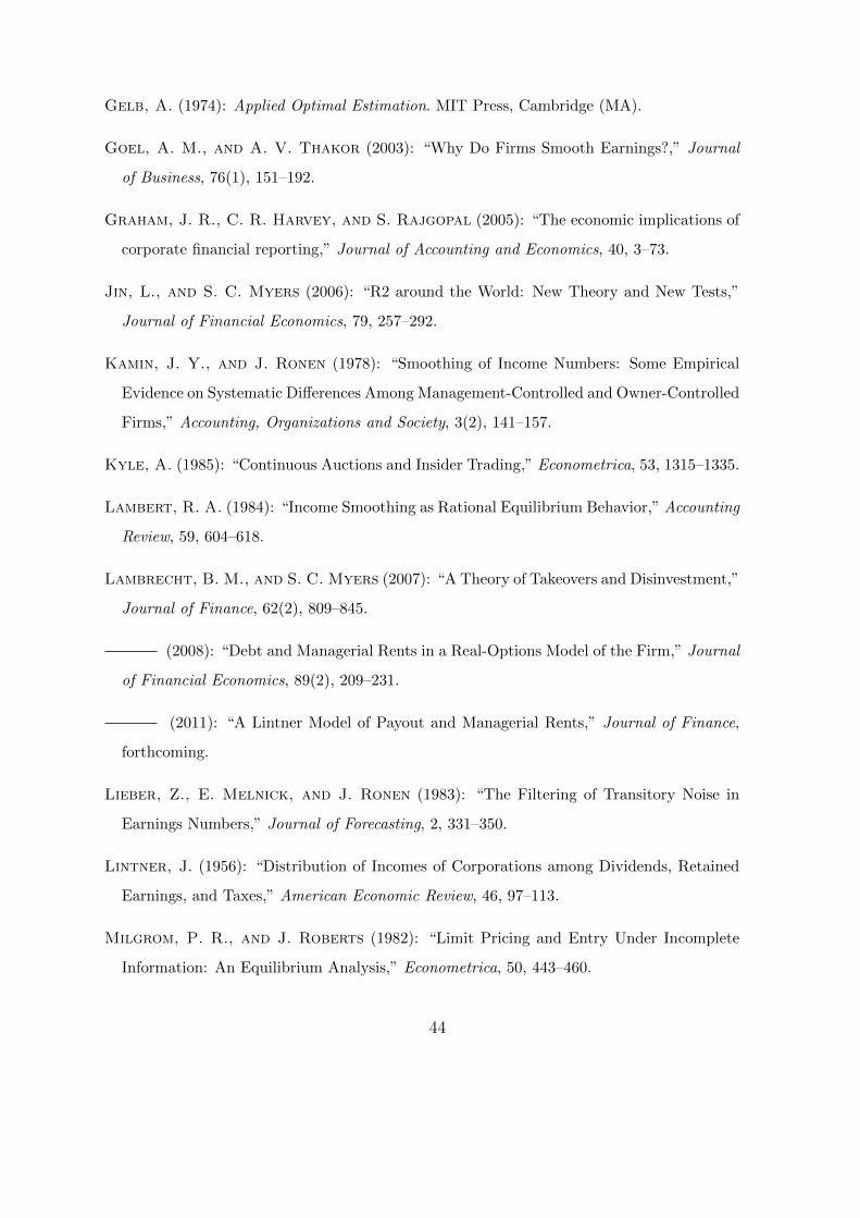
Figure 1 illustrates the effect of the key model parameters (R,Q,A and θ) on

production efficiency.23 Efficiency is measured with respect to 3 different variables:

effort (et), the unconditional mean output (E[qt]), and unconditional mean income

(E[πt]). The degree of efficiency is determined by comparing the actual outcome with

the first-best outcome, i.e., et/eo (solid line), E[qt]/E[qot ] (dashed line), and E[πt]/E[πot ]

21For R = 0 we get P = Q, K = 1/H and λ = 0. Therefore, from Proposition 2 it follows that

x̂t = st/H and st = Hxt. Consequently, x̂t = xt.22Formally, to analyze the behavior of H for R = 0 as a function of θ, we calculate:

∂H

∂θ= − 2

(2− θ)2< 0 and

∂2H

∂θ2= − 4

(2− θ)3< 0 (23)

It follows that H is a concave declining function of θ when R = 0. In other words, H declines at

an increasing rate. This implies that the production and effort policies become more inefficient at an

increasing rate as insiders’ ownership stake is eroded.23The baseline parameter values used to generate all the figures in this paper are: A = 0.8, B = 1,

c = 1, Q = 4, R = 1, β = 0.95 and θ = 0.8.

18

(dotted line).

The figure shows that the efficiency loss is always largest with respect to output

and smallest with respect to effort, with income falling in between because the loss in

revenues is to some extent offset by lower costs of effort and production. Panel A and

B confirm that full efficiency is achieved as R moves towards∞ and for Q = 0. Panel C

shows that a higher autocorrelation in marginal costs substantially reduces efficiency

because it allows outsiders to infer more information about the latent cost variable

from sales and therefore gives insiders stronger incentives to distort production.

Finally, panel D shows that production is fully efficient if outsiders have no stake in

the firm’s income (i.e., θ = 0). Efficiency severely declines as outsiders’ stake increases.

For θ = 1, insiders have no real ownership stake in the firm but they are still expected

to determine production policy and to pay out the expected income. We know from

our earlier analysis that insiders stop producing altogether if sales are fully informative

(i.e., H = 0 if R = 0 or Q =∞). However, if sales are not fully informative (as is the

case for our benchmark parameter values), then this leaves some scope for insiders to

“hide” their actions. Insiders therefore still benefit to some degree by putting in a bit

of effort. For our baseline parameter values insiders’ incentives are seriously eroded as

they put in only 13% of the first-best effort level and achieve only 5% of the first-best

output level for θ = 1. However, one can show that as Q/R → 0 incentives are fully

restored, and the first-best outcome can be achieved even for θ = 1. This confirms

that the root cause of underproduction is the process of indirect inference and not the

outside ownership stake per se. The firm’s ownership structure serves, however, as a

transmission mechanism through which inefficiencies can be amplified.

2.2 The time-series properties of income

Proposition 2 also allows us to derive the time-series properties of income:

Proposition 3 The firm’s “actual income” is:

πt = hxt −1

2c e2. (24)

19

The firm’s “reported income” is described by the following target adjustment model.

π̂t = ES,t[πt] = hx̂t −1

2c e2 (25)

= π̂t−1 + (1− λA) (π∗t − π̂t−1) (26)

= λAπ̂t−1 + KH

(1− H

2

)st + k ≡ γ̂0 + γ̂1 st + γ̂2π̂t−1 . (27)

The “income target” π∗t is given by:

π∗t =k

1− λA+

(KH

1− λA

)(1− H

2

)st ≡ γ∗0 + γ∗1 st . (28)

where k ≡ hλBe − 12ce2 (1− λA) and where h ≡

(H − H2

2

). The speed of adjustment

coefficient is given by SOA ≡ (1− λA) with 0 < SOA ≤ 1.

The proposition characterizes three types of income: the “income target” (π∗t ), “re-

ported income” (π̂t) and “actual income” (πt). Reported income follows a target that is

determined by the contemporaneous level of sales. However, as equation (26) shows, the

reported income only gradually adjusts to changes in sales because the SOA coefficient

(1− λA) is less than unity. This leads to income smoothing in the sense that the effect

on reported income of a shock to sales is distributed over time. In particular, a dollar in-

crease in sales leads to an immediate increase in reported income of only(H − H2

2

)K.

The lagged incremental effects in subsequent periods are given by(H − H2

2

)KλA,(

H − H2

2

)K(λA)2,

(H − H2

2

)K(λA)3,... The long-run effect of a dollar increase in

sales on reported income equals(H − H2

2

)K∑∞

j=0 (λA)j =

(H−H2

2

)K

1−λA , which is the

slope coefficient γ∗1 of the income target π∗t (see equation (28)). In contrast, with sym-

metric information, the impact of a shock to sales is fully impounded into reported

income immediately.

Our model for reported income can also be expressed as a distributed lag model

in which reported income is a function of current and past sales. Indeed, repeated

backward substitution of equation (27) gives:

π̂t =k

1− λA+ Kh

∞∑j=0

(λA)j st−j . (29)

Given that (i) reported income is smooth relative to actual income and (ii) payout is

based on reported income, it follows that insiders soak up the variation. We return to

this issue in Section 2.4, where we discuss payout.

20

2.3 Income smoothing

We now consider the smoothing mechanism in more detail. Our model identifies two

types of shocks: value-irrelevant transitory measurement errors (εt) and value-relevant

persistent shocks to marginal costs (wt). We now explore in turn the effect of each

type of shock on the various income measures.

2.3.1 Transitory measurement errors

The following corollary summarizes the effects of measurement errors.

Corollary 4 Measurement errors create asymmetric information, which in turn leads

to smoothing of reported income. The effect of a measurement error εt on actual income

(πt), reported income (π̂t) and the income target (π∗t ) is as follows:

∂πt+j∂εt

= 0 for all j ≥ 0 (30)

∂π̂t+j∂εt

= Kh (λA)j for all j ≥ 0 (31)

∂π∗t+j∂εt

=Khδj

1− λAwhere δj = 1 if j = 0 and δj = 0 if j > 0 (32)

∞∑j=0

∂π∗t+j∂ε

=∂π∗t∂εt

=Kh

1− λA=

∞∑j=0

∂π̂t+j∂εt

(33)

Measurement errors are not value-relevant and therefore do not affect actual income

(i.e.∂πt+j

∂εt= 0). Measurement errors do affect outsiders’ beliefs about income and

therefore also reported income. Their effect is, however, distributed over time, i.e.

reported income smooths out transitory measurement errors. In contrast, the income

target instantaneously impounds the aggregate effect of measurement errors (i.e.,∂π∗t∂εt

=∑∞j=0

∂π̂t+j

∂εt). Since measurement errors are value-irrelevant noise and merely affect

current sales there is no reason why they should affect future income targets. The

presence of measurement errors (and therefore asymmetric information) is a necessary

condition to have income smoothing.24

24Formally, λ ≥ 0 ⇐⇒ R ≥ 0. If R = 0 then SOA = 1 and reported income fully adjust each

period to the target. Full adjustment also occurs if the marginal cost variable is uncorrelated, even

21

2.3.2 Persistent shocks to marginal costs.

The following corollary summarizes the effects of persistent shocks to the marginal cost

variable xt.

Corollary 5 The effect of a persistent shock wt−1 in the latent cost variable on actual

income (πt), reported income (π̂t) and the income target (π∗t ) is as follows:

∂πt+j∂wt−1

= hAj (34)

∂π̂t+j∂wt−1

=KhHAj(1− λj+1)

(1− λ)(35)

∂π∗t+j∂wt−1

=

(KH

1− λA

)hAj (36)

∞∑j=0

∂π∗t+j∂wt−1

=KHh

(1− λA)(1− A)=

∞∑j=0

∂π̂t+j∂wt−1

(37)

A persistent shock to income arises from a shock to the firm’s marginal cost of produc-

tion, and affects both contemporaneous and future income (∂πt+j

∂wt−1= hAj) because the

marginal cost variable is autoregressive (A > 0). The cumulative effect on actual in-

come of a persistent shock equals∑∞

j=0∂πt+j

∂wt−1= h

1−A . In terms of targets, a persistent

shock affects all future income targets due to the autoregressive nature of marginal

production costs. And, with regard to reported income, the effect of a persistent shock

is smoothed over time because in the short run outsiders cannot distinguish between

measurement error and shocks to the latent cost variable. As time passes, it becomes

gradually clear whether a shock in sales was due to measurement error or a change

in the latent marginal cost variable. Therefore, the total aggregate effect on reported

income adds up to the total effect on the income target. In other words, although

reported income initially adjust more slowly than the income target, reported income

“catches up” eventually so that over the long run it impounds the full aggregate effect.

The SOA to the income target decreases as Q, the variance of persistent shocks

wt, decreases. As Q → 0, K converges to 0, and therefore λ converges to 1, and

SOA→ 1−A. From Proposition 3, it follows that reported income no longer depend

if there is transitory noise (i.e., SOA = 1 if A = 0). And, when the variance of measurement errors

becomes infinite, the SOA converges to 1−A.

22

on sales. In other words, outsiders do not learn from sales because the dynamic behavior

of the latent cost variable is deterministic and fully known to outsiders.

2.3.3 The effect of information asymmetry on income smoothing

Corollary 6 A lower degree of information asymmetry (i.e., R falls relative to Q)

leads to less smoothing. In the limit (i.e., R = 0 or Q→∞) both reported income and

target income coincide with actual income at all times (i.e., πt = π̂t = π∗t for all t).25

No smoothing whatsoever occurs when R = 0 because in that case all information

asymmetry is eliminated. In the absence of measurement errors, it is possible to infer

the marginal cost variable xt with 100% accuracy from the observed sales figure st.

The same result obtains when Q → ∞ because in that case measurement errors are

negligibly small compared to the variance of the latent cost variable. This important

result confirms again that asymmetric information and not uncertainty per se is the

root cause of income smoothing.

The corollary also confirms that as the degree of information asymmetry goes to

zero, our rational expectations equilibrium converges to the simple sharing rule that

prevails under symmetric information. Indeed: limR→0 dt = θ limR→0 π̂t = θπt.

Consider now the other polar case where sales are extremely noisy measures of the

latent cost variable (i.e., R → +∞). One can verify that reported income now evolve

according to an AR(1) process:

π̂t = Aπ̂t−1 +Be

2− 1

2ce2(1− A) (38)

Therefore, in this case, reported income evolves according to the (expected value of

the) AR(1) process for the latent cost variable. Sales no longer provide any additional

information and measurement errors no longer affect reported income.

A similar result applies when the process for the latent cost variable becomes deter-

ministic (Q = 0). One can verify that in that case the process for reported income is

25For R = 0 we obtain K = 1/H and λ = 0, and as a result, we get γ̂1 = γ∗1 = − 12ce

2 and

γ̂0 st = γ∗1 st = hxt, and therefore πt = π̂t = π∗t .

23

again described by (38). Since xt is deterministic, its evolution can be described with

100% accuracy. Sales again become irrelevant towards determining reported income

and, as a result, measurement errors play no role. This leads to the following corollary:

Corollary 7 If measurement errors become extremely large (R = +∞) or if there are

no persistent shocks to the latent cost variable (Q = 0) then reported income behaves

according to (the expected value of) the process for the latent cost variable. Sales figures

do not affect reported income.

2.3.4 Real versus financial smoothing.

Figure 2 illustrates and summarizes the effect of the main model parameters (θ, A,R

and Q) on the speed of adjustment (SOA) of reported income to the income target.

Recall that no smoothing (i.e., SOA = 1) occurs under symmetric information. Our

symmetric information benchmark case corresponds therefore with SOA = 1 (repre-

sented by a solid horizontal line at SOA = 1 in the figure). The dotted line plots

the SOA that results from the actual production policy (as determined by H) derived

under asymmetric information. While this gives us an idea of the total amount of

intertemporal income smoothing, it does not tell us how much of this is due to the

suboptimal production policy that results from indirect inference and how much is due

to mere financial smoothing that results from asymmetric information. We refer to the

former as “real” smoothing and to the latter as “financial” smoothing.

The financial smoothing component is measured by evaluating the SOA at the

first-best production policy H = 1, i.e. SOA = 1 − Aλ[H = 1] (as represented by

the dashed line). Therefore Aλ[H = 1] reflects the amount of smoothing that would

take place under asymmetric information but assuming that insiders were to adopt

the efficient production policy. Financial smoothing is therefore measured in figure

2 by the distance between the horizontal solid line at SOA=1 and the dashed line.

Since the dotted line represents the total amount of smoothing (i.e., financial plus

real smoothing), the difference between the dashed line and the dotted line (given by

Aλ− Aλ[H = 1]) captures the amount of “real smoothing”.

24

The distinction between the two types of smoothing is clearly illustrated in panel A

which plots the SOAs as a function of the (real) outside ownership stake θ. Changing θ

does not alter the degree of asymmetric information between insiders and outsiders and,

as a result, the amount of financial smoothing remains constant. The corresponding

SOA of 0.86 (dashed line) implies a half-life of about 0.35 years for adjustment of

reported income to changes in sales.26 Increasing θ introduces, however, additional

real smoothing and this reduces the SOA from 0.86 (for θ = 0) to 0.56 (for θ = 1)

corresponding, respectively, to a half-life of 0.35 years and 0.84 years. In the latter case

real smoothing adds about half a year to the half-life. The plot confirms our earlier

results that reducing inside ownership leads to severe underproduction, which in turn

leads to a smoother reported income flow because income becomes less sensitive to

sales.

Panel B shows that smoothing also increases with the degree of autocorrelation in

the latent cost variable. No intertemporal smoothing takes place when A = 0 because

in that case current and past realizations of xt are irrelevant for the future. As a result,

insiders’ private information about xt is also irrelevant for the future. Note that higher

autocorrelation raises both real and financial smoothing substantially.

Finally, panels C and D confirm that the total amount of smoothing increases with

the degree of information asymmetry (as reflected by a higher R or lower Q). Para-

doxically, more intertemporal smoothing coincides with higher production efficiency

(see figure 1): when outsiders can infer less from sales, there is also less of an incen-

tive to manipulate production. Note that a higher degree of information asymmetry

unambiguously increases the amount of financial smoothing.

2.4 Payout Policy

Since the payout to outsiders is given by dt = θπ̂t, it follows that the firm’s payout

policy to outsiders is described by the target adjustment model for π̂t in (27):

dt = λAdt−1 + θhKst + θk . (39)

26Half-life is the time needed to close the gap between reported income and the income target by

50%, after a one-unit shock to the error term in the target adjustment model for reported income.

When reported income follows an AR(1) process half-life is log(0.5)/ log(1 - SOA).

25

The payout model is similar to the well known Lintner (1956) dividend model. The

key difference is that in Lintner (1956) the payout target is determined by the firm’s

net income, whereas in our model the target is a function of sales because net income

is not directly observable by outsiders. Payout in our model is not smoothed relative

to reported income but relative to a proxy variable observable by outsiders, i.e. sales.27

3 Robustness, extensions and discussion

3.1 Forced disclosure and the “big bath”

Insiders’ payout policy guarantees that the capital market constraint is satisfied at all

times, i.e., St ≥ ϕαEt[Vt|It]. But will insiders be willing to adhere to this payout

policy under all circumstances? Insiders’ participation constraint is satisfied if they

are better off paying out than triggering collective action. Collective action implies

that stockholders “open up” the firm and uncover its true value (Vt). It is reasonable

(although not necessary) to assume that collective action also imposes a cost upon

insiders. Graham et al. (2005) report that the consequences of missing an earnings

target can be so serious for managers’ career and reputation that they try to avoid

missing the target at all cost. Without loss of generality assume that these costs are

proportional to the firm value and given by Ct = cVt.

Insiders trigger collective action when outsiders’ beliefs regarding the firm’s value

(and therefore the required payout) are excessively overoptimistic. “Forced disclosure”

by outsiders pricks the bubble that has been building up over time and brings outsiders’

beliefs about the firm value back to reality, i.e. Et[Vt|It] = Vt.

A sufficient (but not necessary) condition for insiders to keep paying out according

27Payout smoothing in the strict Lintner sense could be obtained, for instance, if insiders are risk-

averse and subject to habit formation. Lambrecht and Myers (2011) show that insiders of this type

smooth payout relative to income by borrowing and lending. Introducing debt and cash into our

model would allow risk-averse insiders to borrow against future income or to “park” reported income

onto the firm’s cash account (see also footnote 11).

26

to outsiders’ expectations is:

Mt = Vt − ϕαEt[Vt|It] ≥ Vt − ϕαVt − cVt ⇐⇒ Vt ≥ ϕααϕ+c

Et[Vt|It] (40)

Therefore, outsiders have an incentive to trigger collective action if the firm’s actual

value (Vt) drops sufficiently below below what outsiders believe the firm to be worth

(Et[Vt|It]).28 This situation arises if outsiders’ beliefs about the latent cost variable (as

reflected by x̂t) are overoptimistic due to measurement errors.29

As mentioned before, insiders absorb the variation between actual and reported

income. In particular, each period insiders actually receive (πt − ϕαπ̂t) instead of

(1 − ϕα)πt. The net gain (or loss) to insiders is therefore ϕα (πt − π̂t). The net gain

relative to the actual amount received is ϕα(πt − π̂t)/(πt − ϕαπ̂t). For a small outside

ownership stake (e.g., private firms) or a low degree of investor protection (α), the gain

or loss that insiders absorb is only a small fraction of the income stream they receive.

However, as ϕ→ 1 and α→ 1, these gains πt − π̂t constitute 100% of insiders’ income.

How can one reduce the likelihood of costly forced disclosure? Since a lower nominal

inside ownership stake (ϕ) and a lower degree of investor protection (α) relax insiders’

participation constraint, one obvious solution is to reduce either of these two (or a

combination of both).30 Unfortunately, this also reduces the firm’s capacity to raise

outside equity. Therefore, firms that rely heavily on outside equity (e.g. public firms)

adopt more efficient (in terms of cost and speed) disclosure mechanisms such as volun-

tary audited disclosure. While “big baths” do occur in reality, they rarely result from a

very costly forced disclosure process but they are much more likely to happen through

the process of regular voluntary audited disclosures.31 As we show below, high quality

audited disclosures keep misvaluations within bounds and resolve the need for insiders

28Calculating the exact condition under which insiders optimally exercise their option to trigger

collective action is beyond the scope of this paper.29Note that measurement errors as such do not jeopardize the actual economic viability of the firm

because measurement errors are value-irrelevant (even though they can induce temporary misvalu-

ations in the firm’s stock price). Therefore, in our model a “big bath” would never coincide with

bankruptcy or actual abandonment by insiders because actual firm value is always strictly positive in

our model.30Non-pecuniary private benefits of control may also play a role in keeping insiders on board.31One important exception is the case of deliberate fraud which, by its very nature, often requires

legal investigative teams with special powers to uncover the truth.

27

to trigger collective action and force disclosure. Still, in many countries with weak gov-

ernance, reliable accounting information may not be available and outsiders’ property

rights may be hard to enforce, explaining the widespread phenomenon of family firms

with a high insider ownership stake and a low degree of investor protection.

3.2 Audited disclosure and ownership structure

Our analysis in section 2 showed that the firm’s effort and production policy become

increasingly more inefficient as insiders’ real ownership stake (1− ϕα) decreases. This

could pose serious problems for public firms, which often have a small inside equity

base and a large number of highly dispersed outside shareholders. Our model predicts

that under-investment could become so severe that firms stop producing altogether,

even if they are inherently profitable.

It may therefore come as no surprise that mechanisms have been developed to

reduce the degree of information asymmetry. In particular, publicly traded companies

(unlike private firms) are subject to stringent disclosure requirements.32 The traditional

argument put forward to justify disclosure is often that of investor protection. The

general underlying idea is that outside investors need to be protected from fraud or

conflicts of interests by insiders (usually managers). Audited disclosure is generally

believed to benefit outsiders by curtailing insiders’ ability to exploit their informational

advantage and to extract informational rents.

Our paper shows that the case for audited accounting information rests not only

on investor protection. Our model shows that asymmetric information is problematic

even if insider trading is precluded and outsiders’ property rights are 100% guaranteed

(i.e., α = 1). Moreover, disclosure is not necessarily a win/lose situation for out-

siders/insiders. In our setting, eliminating information asymmetry would be welcomed

by outsiders and insiders alike. In other words, disclosure (assuming it can be achieved

in a relatively costless fashion) is a win-win situation for all parties involved.

32While a private firm has no requirement publicly to disclose much, if any, financial information,

public firms are required to submit an annual form (Form 10-K in the United States, for instance)

giving comprehensive detail of the company’s performance. Public firms are also required to spend

more on independent, certified public accountants and they are subject to much more laws and

regulations (such as the Securities Act of 1933 and the 2002 Sarbanes-Oxley Act in the U.S.).

28

Formally, in proposition 2 we showed that, on the basis of current and past sales,

outsiders calculate an income estimate π̂t. The error of outsiders’ estimate, πt − π̂t, is

normally distributed with zero mean and variance σ̂2. Suppose now that, in addition

to the sales data, auditors provide each period an independent estimate yt of income

where yt ∼ N(πt, σ2). Importantly, auditors provide their assessment after εt and wt−1

are realized. The auditors’ estimate is unbiased (i.e., Et[yt] = πt)33 but subject to some

random error (yt− πt). Insiders nor auditors have control over the error, and the error

is independent across periods. In summary, on the basis of the full sales history It

outsiders construct a prior distribution of current income that is given by N(π̂t, σ̂2).

Auditors then provide an independent estimate yt, which outsiders know is drawn from

a distribution N(πt, σ2).

Using simple Bayesian updating, it follows that the outsiders’ estimate of income

conditional on yt and on the sales history It is given by:34

κyt + (1− κ)π̂t where κ =σ̂2

σ̂2 + σ2. (41)

The parameter κ can be interpreted as a parameter that reflects the quality of the

additional information provided. A value of κ close to 0 means that the audited

disclosure is highly unreliable and carries little weight in influencing outsiders’ beliefs

about income.

How does the provision of information by independent auditors influence insiders’

decisions? Insiders’ optimization problem can now be formulated as:

Mt = maxqt+j ,et+j ;j=0..∞

Et

[∞∑j=0

βj (π(qt+j, et+j) − ϕακEt+j(yt+j) − ϕα(1− κ)ES,t+j [π (qt+j, et+j)])

]

= maxqt+j ,et+j ;j=0..∞

Et

[∞∑j=0

βj (π(qt+j, et+j) (1− ϕακ) − ϕα(1− κ)ES,t+j [π (qt+j, et+j)])

]

= (1− ϕακ) maxqt+j ,et+j ;j=0..∞

Et

[∞∑j=0

βj (π(qt+j, et+j) − G(ϕ, α, θ)ES,t+j [π (qt+j, et+j)])

](42)

33This assumption is not strictly necessary. For example, if auditors are, say, conservative then the

analysis would remain similar provided that outsiders know the auditors’ bias.34It might be possible for outsiders to refine the estimate of the latent cost variable xt by using the

entire history of auditors’ income estimates. We ignore this possibility, and assume that all relevant

accounting information is encapsulated in the auditors’ most recent income estimate.

29

where G(ϕ, α, κ) ≡ ϕα(1−κ)1−ϕακ ≡ θ(1−κ)

1−θκ , and where we made use of the fact that the

auditors’ estimate is unbiased at all times, i.e., Et+j[yt+j] = π(qt+j, et+j) for all j,

irrespective of insiders’ decision rules for qt+j and et+j. In other words, insiders can-

not distort auditors’ estimate (the release of the accounting information happens by

independent auditors after income are realized).

Comparing the optimization problem (42) with the original one we solved in (9),

one can see that both problems are essentially the same, except for the fact that

the outside ownership parameter θ in (9) has been replaced by the governance index

G(ϕ, α, κ) in (42). This means that the solutions for qt+j and et+j can be obtained by

merely replacing θ by G(ϕ, α, κ) in the solution we previously obtained.

G(ϕ, α, κ) ranges across the [0, 1] interval and can be interpreted as an (inverse)

governance index that crucially depends on the outsiders’ ownership stake (ϕ), the

degree of investor protection (α) and on the quality of audited disclosure (κ). If κ = 0

(i.e., G = θ) then the independently provided accounting information is completely

unreliable and discarded by outsiders. In that case the optimization problem and

its solution coincide exactly with the ones presented in section 2. If κ = 1 (i.e.,

G = 0) then the independently provided accounting information is perfectly reliable.

All information asymmetry is resolved and we get the first-best outcome that was

presented in section 1.

Calculating the comparative statics for G with respect to θ and κ gives:

∂G(θ, κ)

∂θ=

1− κ[1− θκ]2

≥ 0 , and∂G(θ, κ)

∂κ=

θ(θ − 1)

[1− θκ]2≤ 0 .

It follows that reducing outsiders’ (real) equity stake or increasing the quality of audited

disclosure act in a similar fashion, and these levers are therefore substitutes. The results

are summarized in the following corollary:

Corollary 8 Higher quality audited disclosure (κ) improves the firm’s operating effi-

ciency and acts as a substitute for a higher real inside ownership stake (θ).

30

3.3 Accounting quality, stock market size and growth

In this section we examine the model’s implications for corporate investment (and

economic growth more generally) by analyzing the initial decision to set up the firm.

Assume that an investment cost E is required to establish the firm at time t =

0. The financing is raised from inside and outside equity. To abstract from adverse

selection issues (see Myers and Majluf (1984)) we assume as before that insiders have

access to an unbiased estimate for x0 at time zero (i.e., x̂0 = x0). As a result insiders

and outsiders attach the same value V (x0; θ, κ) to the firm when the firm is founded,

as given in the following proposition.

Proposition 4 The value of the firm at time t = 0 is given by:

V0(x0; θ, κ) =h

(1− βA)

(x0 +

Beβ

1− β

)− 1

2

ce2

(1− β)(43)

where the values for the production (h ≡ H − H2

2) and effort (e) policies are obtained

as described in proposition 2 but by replacing θ everywhere by G(θ;κ).

We know that the firm value monotonically declines in the real ownership stake θ(≡αϕ). Therefore the first-best firm value is achieved when the outside ownership stake

is zero (i.e., θ = 0). Assuming the investment in the firm happens on a now-or-never

basis at t = 0, the first-best investment decision is given by the following criterion:

invest if and only if V (x0; θ = 0, κ) ≥ E. Note that the accounting quality κ does

not influence the investment decision when θ = 0, because without outside investors

audited disclosure becomes superfluous.

Assume next, without loss of generality, that insiders have no money to contribute

and need to raise the full amount E from outsiders. Assume further that the quality

of audited disclosure (κ) is exogenously given, but that the real ownership stake θ can

be chosen.35 The decision problem is therefore to identify the lowest value for θ that

allows insiders to raise enough outside equity, St, to cover the investment cost (i.e.,

S0(x0; θ, κ) = E).

35Outsiders’ nominal ownership stake ϕ is obviously a control variable. The degree of investment

protection α is, initially at least, under control too through the firm’s charter and governance mech-

anisms (such as board composition) that are implemented upon the firm’s foundation.

31

Since x̂0 = x0, the initial inside (M0) and outside (S0) equity are:

M0 = V0(x0; θ, κ)− θES,0 [V0(x̂0; θ, κ)] = (1− θ)V0(x0; θ, κ) (44)

S0 = θES,0 [V0(x̂0; θ, κ)] = θV0(x0; θ, κ) (45)

The (constrained) optimal value for θ is therefore the solution to:

θo = min {θ| θV0(x0; θ, κ) = E} (46)

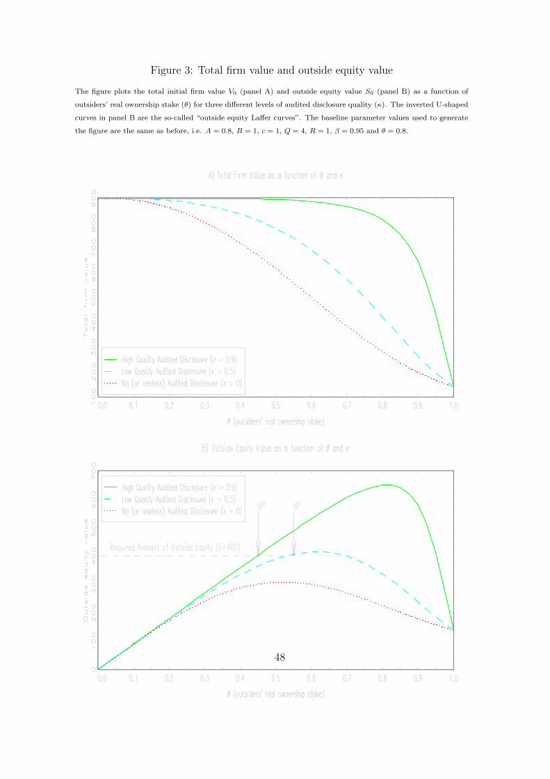
The solution is illustrated in Figure 3. Panel A plots the total firm value V0(x0; θ, κ) as

a function of outsiders’ real ownership θ for three different levels of disclosure quality

(κ). In line with our earlier results, total firm value declines monotonically with respect

to θ. The loss can be substantial: the first-best firm value equals 900 (i.e., for θ = 0),

whereas the firm value under 100% outside ownership equals a mere 150 (i.e., for θ = 1).

High quality audited disclosure (κ = 0.9) can, however, significantly mitigate the value

loss. For example for κ = 0.9 the loss in value appears to be less than 1% for as long

as insiders own a majority stake. In the absence of audited disclosure or when audited

disclosure is completely useless (i.e., κ = 0), significant value losses kick in at much

lower outside ownership levels. For example, at θ = 0.5 about a third of the first-best

value is lost in the absence of audited disclosure.

Panel B shows the total outside equity value as a function of the outside ownership

stake for three different levels of disclosure quality. The curves resemble “outside equity

Laffer curves”.36 The outside equity value θV0(x0; θ, κ) is an inverted U-shaped function

function of θ that reaches a unique maximum. This maximum changes significantly

according to the quality of the audited disclosure, and equals about 650, 420 and 310

for high quality, low quality and no audited disclosure, respectively. No investment

would take place in the absence of audited disclosure, because the amount of outside

equity that can be raised is inadequate to finance the investment cost. Investment

would take place in the two case where accounting information is audited, and about

θo = 45% (θo′

= 55%) of shares would end up in outsiders’ hands with high (low)

quality audited disclosure.

Our results provide theoretical support for a number of empirical studies that have

found a positive link between economic growth, stock market size, stock market capi-

talizations, and quality of accounting information. The standard explanation for this

36The traditional Laffer curve is a graphical representation of the relation between government

revenue raised by taxation and all possible rates of taxation. The curve resembles an inverted U-

shaped function that reaches a maximum at an interior rate of taxation.

32

result is that higher quality accounting information provides better investor protection.

While higher investor protection (i.e., higher α) also leads to higher stock market val-

uations in our model, audited disclosure does not as such improve investor protection

in our model. Instead, independent audited disclosure reduces the inefficiencies from

indirect inference because insiders are less concerned about the effect of their actions

on outsiders’ expectations. Our model therefore highlights an important role of inde-

pendent audited disclosure and monitoring that has hitherto not been recognized in

the literature.37 Figure 3 illustrates that the efficiency gains from audited disclosure

can be economically highly significant.

4 Additional empirical implications

Our theory of intertemporal income smoothing yields rich, testable implications for

the time-series properties of reported income and payout to outsiders. Some of these

were outlined in the introductory remarks. Here, we provide some more specific cross-

sectional implications:

First, asymmetric information is the key driver of income smoothing in our model.

Such smoothing implies that reported income follows a target adjustment process.

A testable implication is that, in the cross-section of firms, the speed of adjustment

towards the income target should decrease with the degree of information asymmetry

between inside and outside investors.

Second, asymmetric information and the resulting inference process also lead to

underproduction by firms. Both the degree of underproduction and income smoothing

should increase in the cross-section of firms as outside ownership increases. Therefore,

all else equal, public firms are expected to smooth income more and they suffer more

from under-investment. Kamin and Ronen (1978) and Amihud, Kamin, and Ronen

(1983) show that owner-controlled firms do not smooth as much as manager-controlled

37There is, however, a dark side to monitoring that we ignore in this paper. Burkart, Gromb, and

Panunzi (1997) show that monitoring and tight control by shareholders creates an ex-ante hold-up

threat which reduces managerial initiative and non-contractual investment. A dispersed ownership

structure dilutes the hold-up threat and this gain has to be weighed against the loss in productive

efficiency due to inadequate monitoring and disclosure.

33

firms. Prencipe, Bar-Yosef, Mazzola, and Pozza (2011) also provide direct evidence for

this. They find that income smoothing is less likely among family-controlled companies

than non-family-controlled companies in a set of Italian firms. The implication on

under-investment is unique to our model as it implies real smoothing but to the best of

our knowledge, this has not yet been thoroughly tested. There is, however, convincing

survey evidence by Graham et al. (2005) that a large majority of managers are willing

to postpone or forgo positive NPV projects in order to smooth earnings.

Third, since smoother income leads to smoother payout, one would expect, all else

equal, that public firms also smooth payout more than private firms. This implication

is consistent with Roberts and Michaely (2007) who show that private firms smooth

dividends less than their public counterparts.

Fourth, income figures that are independently provided by auditors improve pro-

duction efficiency because it reduces insiders’ incentives to manipulate income through

their production and effort policy. Thus, all else equal higher quality accounting infor-

mation should increase firm productivity, managerial effort, stock market capitaliza-

tion, and, more generally, economic growth (as confirmed, for instance, by Rajan and

Zingales, 1998).

Finally, firms that do not have access to independent and high quality auditors can

issue less outside equity. Our model therefore predicts that inside ownership stakes

should be greater in countries with weaker quality of accounting information, which

appears consistent with the widespread phenomenon of greater private and family firms

in such countries.

5 Related literature

Our paper belongs to a series of papers (Fluck (1998, 1999), Myers (2000), Jin and My-

ers (2006) and Lambrecht and Myers (2007, 2008, 2011)) where insiders make payouts

to avoid collective action by outsiders. With the exception of Jin and Myers (2006)

these papers assume symmetric information between insiders and outsiders. In Jin and

Myers, insiders pay out according to outsiders’ expectations of cashflows and absorb

the variation, as is also the case in our model. Their model differs, however, in a num-

ber of fundamental ways. Insiders do not make any production or effort decisions in Jin

34

and Myers. Their cash-flow process is completely exogenous and contains a component

that is only observable to insiders. Outsiders do not learn about the latent component

and, as a result, there is no intertemporal smoothing in their model.

Our model of intertemporal smoothing by a firm’s insiders also provides theoretical

support for the Lintner (1956) model of smooth payout policy. To our knowledge, it

is only the second model to do so after Lambrecht and Myers (2011). Lambrecht and

Myers (2011) assume a complete information setting where managers set payout policy

and their own compensation. But, managers’ compensation is tied to payout because

of a threat of collective action by shareholders. Managers’ risk aversion and habit

formation induces them to smooth their rents (and, therefore also payout) relative to

net income. Our model does not explain why payout is smooth relative to income,

but instead explains why income is smooth in the first place. As such, our model is

complementary to the one of Lambrecht and Myers (2011). Importantly, while risk

aversion is a pervasive ingredient in existing papers on income and payout smoothing,

our paper does not rely on risk aversion to generate intertemporal smoothing.

An early, very comprehensive discussion of the objectives, means and implications

of income smoothing can be found in the book by Ronen and Sadan (1981) (which

includes references to some of the earliest work on the subject). In Lambert (1984)

and Dye (1988) risk-averse managers without access to capital markets want to smooth

the firm’s reported income in order to provide themselves with insurance.38 Fudenberg

and Tirole (1995) develop a model where reported income is paid out as dividends and

where risk-averse managers enjoy private benefits from running the firm but can be

fired after poor performance. They assume that recent income observations are more

informative about the prospects of the firm than older ones. They show that managers

distort reported income to maximize the expected length of their tenure: managers

boost (save) income in bad (good) times.

There are also signaling and information-based models to explain income smooth-

ing. Ronen and Sadan (1981) employ a signaling framework to argue that only firms

with good future prospects smooth earnings because borrowing from the future could

be disastrous to a poorly performing firm when the problem explodes in the near term.

38Models driven by risk-aversion (or limited liability) of managers naturally lead to considering

optimal compensation schemes and how they affect smoothing, but we have excluded this literature

for sake of brevity.

35

Trueman and Titman (1988) also argue that managers smooth income to convince

potential debtholders that income has lower volatility in order to reduce the cost of

debt. Smoothing costs arise from higher taxes and auditing costs. Tucker and Zarowin

(2006) provide evidence that the change in the current stock price of higher-smoothing

firms contains more information about their future earnings than does the change in

the stock price of lower-smoothing firms. Our model assumes that there are at least

some limits to perfect signaling and is in this sense complementary to these alternative

explanations for earnings smoothing.39

The rational expectations equilibrium of our model works as follows. Upon ob-

serving higher sales, outsiders want higher payout. In an attempt to “fool” outsiders,

insiders underproduce (resulting in real smoothing). However, outsiders anticipate this,

and therefore in equilibrium insiders do not succeed in their attempt. Nevertheless,

the indirect inference process distorts corporate choices. This informational effect is

similar to the ones discussed (albeit in different economic settings) in Milgrom and

Roberts (1982), Riordan (1985), Gal-Or (1987), Stein (1989), and more recently Bag-

noli and Watts (2010).40 The learning process (which we model as a filtering problem)

and the intertemporal smoothing mechanism are, however, quite different from existing

papers. The inference model we consider is also fundamentally different from alterna-

tive information models in the accounting and financial economics literature in which a

firm’s disclosures are always fully verifiable and the firm simply chooses whether to dis-

close or not. Disclosure games (see, for instance, Dye (1985, 1990), and more recently,

Acharya, DeMarzo and Kremer (2011)) in which insiders can send imperfect signals

and alter production to affect outsiders’ inference could be an interesting avenue for

future research.

39In a slightly different approach to motivating earnings smoothing, Goel and Thakor (2003) develop

a theory in which greater earnings volatility leads to a bigger informational advantage for informed

investors over uninformed investors, so that if sufficiently many current shareholders are uninformed

and may need to trade in the future for liquidity reasons, they want the manager to smooth reported

earnings as much as possible.40While in our model insiders have an incentive not to raise outsiders’ expectations regarding income,

opposite incentives arise in Bagnoli and Watts (2010) who examine the interaction between product

market competition and financial reporting. They show that Cournot competitors bias their financial

reports so as to create the impression that their production costs are lower than they actually are.

36

6 Conclusion

The theory of income smoothing developed in this paper assumes that (i) insiders have

information about income that outside shareholders do not, but (ii) outsiders are en-

dowed with property rights that enables them to take collective action against insiders

if they do not receive a fair payout that meets their expectations. We showed that

insiders report income consistent with outsiders’ expectations based on available in-

formation rather than the true income. This gave rise to a theory of inter-temporal

smoothing – both real and financial – in which observed income and payout adjust

partially and over time towards a target and insiders under-invest in production and

effort. The primary friction driving the smoothing is information asymmetry as in-

siders are averse to choosing actions that would unduly raise outsiders’ expectations

about future income. Interestingly, this problem is more severe the smaller is the inside

ownership and thus should be a greater hindrance to the functioning of publicly (or

dispersedly) owned firms. We show that the firm’s outside equity value is an inverted

U-shaped function of outsiders’ ownership stake. This “outside equity Laffer curve”

shows that the under-investment problem severely limits the firm’s capacity to raise

outside equity. However, a disclosure environment with adequate quality of indepen-

dent auditing can help mitigate the problem, leading to the conclusion that accounting

quality can enhance investments, size of public stock markets and economic growth.

While our theory of inter-temporal smoothing of income and payout conforms to

several existing findings (such as the Lintner (1956) model of payout policy), it also

leads to a range of testable empirical implications in the cross-section of firms as in-

formation asymmetry and ownership structure are varied. These are worthy of further

investigation. It would also be fruitful to apply our framework to other corporate con-

texts so as to investigate the role of capital structure (debt versus equity) in addressing

income smoothing as well as to study how alternative managerial objectives such as

myopia further affect smoothing outcomes.

7 Appendix

Proof of Proposition 1

37

The firm value is given by:

Vt = Et

[∞∑j=0

βj[qt+j −

q2t+j

2xt+j− 1

2ce2t+j

]](47)

The first order conditions with respect to qt and et are:

∂Vt∂qt

= 1 − qtxt

= 0 (48)

∂Vt∂et

= Et

[1

2

(qtxt

)2

B +β

2

(qt+1

xt+1

)2

BA+β2

2

(qt+2

xt+2

)2

BA2 + ...− cet

]= 0(49)

Solving gives the expressions for qt and et as given in the proposition.

We now check the second order condition. The first order leading principal minor

of the Hessian is given by ∂2V∂q2t

= − 1xt< 0. The second order leading principal minor

is given by:

∂2Vt∂q2

t

∂2Vt∂e2

t

−(∂2Vt∂et∂qt

)2

= Et

[c

xt+

B2

xt

[βA2

xt+1

+β2A4

xt+2

+β3A6

xt+3

+β4A8

xt+4

+ ...

]]> 0

(50)

The first and second order leading principal minor of the Hessian are negative and

positive, respectively (assuming a positive cost variable). It follows that the Hessian is

negative definite. Consequently, the critical point is a maximum.

Proof of Proposition 2

Insiders’ optimization problem can be formulated as:

Mt = max{qt+j ,et+j ;j=0..∞}

Et

[∞∑j=0

βj (π(qt+j, et+j) − θES,t+j(π(qt+j, et+j)|It+j))

](51)

where π(qt+j, et+j) = qt+j − 12

q2t+j

xt+j− 1

2ce2t+j and It denotes the information available

to outsiders at time t, i.e., It = {st , st−1 , st−2 , st−3 , ...}. We guess the form of the

solution and use the method of undetermined coefficients (and subsequently verify this

conjecture). The conjectured solution for outsiders’ rational expectations based on the

information It is as follows:

ES,t [π(qt, et)|It] = b +∞∑j=0

ajst−j (52)

38

where the coefficients b and aj(j = 0, 1, ...) remain to be determined.

The first-order conditions are:

∂Mt

∂qt= 1 − qt

xt− θ

(a0 + βa1 + β2a2 + β3a3 + ...

)= 0 (53)

∂Mt

∂et= Et

[1

2

(qtxt

)2

B +β

2

(qt+1

xt+1

)2

BA+β2

2

(qt+2

xt+2

)2

BA2 + ...− cet

]= 0(54)

Combining both conditions gives the optimal output and effort policy:

qt =

[1 − θ

∞∑j=0

ajβj

]xt ≡ Hxt (55)

et =H2B

2c(1− βA)≡ e (56)

Outsiders rationally anticipate these policies and can therefore make inferences about

the latent variable xt on the basis of their observation of current and past sales st−j

(j = 0, 1, ...). We know that st = qt + εt. Consequently, observed sales st are an

imperfect (noisy) measure of the output qt chosen by insiders, and therefore also of the

latent variable xt, as is clear from the following “measurement equation”:

st = H xt + εt with εt ∼ N(0, R) (57)

Outsiders know the variance R of the noise and the parameters A, B and Q of the

“state equation”:

xt = Axt−1 + B e + wt−1 with wt−1 ∼ N(0, Q) for all t (58)

Using a standard Kalman filter the measurement equation can be combined with the

state equation to make inferences about xt on the basis of current and past observations

of st. This, in turn, allows outsiders to form an estimate of realized income πt. It can

be shown that the Kalman filter is the optimal filter (in terms of minimizing the mean

squared error) for the type of problem we are considering (see Chui and Chen (1991)).

We focus on the “steady state” Kalman filter, which is the estimator x̂t for xt that

is obtained after a sufficient number of measurements st have taken place over time

for the estimator to reach a steady state. One can show (see Chui and Chen (1991),

p78) that the error of the steady state estimator, xt − x̂t, is normally distributed

39

with zero mean and variance P , i.e., ES,t[xt − x̂t] = 0 and E[(xt − x̂t)2] = P , or

p(xt|It) ∼ N(x̂t, P ), where x̂t is given by:

x̂t ≡ ESt[xt] = Ax̂t−1 +Be + K [st − H (Ax̂t−1 +Be)] = (Ax̂t−1 +Be)λ + Kst

(59)

where:

λ ≡ (1 − KH) and K ≡ H P

H2P + Rand where P is the positive root of the equation:

P = A2

[1 − H2P

H2P + R

]P + Q (60)

or equivalently, P is the positive root of the equation:

H2P 2 + P[R(1− A2) − QH2

]− QR = 0 (61)

K is called the “Kalman gain” and it plays a crucial role in the updating process.41

Substituting x̂t−1 in (59) by its estimate, one obtains after repeated substitution:

x̂t = eBλ[1 + λA+ λ2A2 + λ3A3 + ...

]+ K

[st + λAst−1 + λ2A2st−2 + λ3A3st−3 + ...

]=

eBλ

1− λA+ K

∞∑j=0

λjAjst−j (62)

Using the conjectured solution for qt it follows that outsiders’ estimate of income

at time t is given by:

ES,t[πt] = ESt

[Hxt −

H2xt2− 1

2ce2

](63)

=

(H − H2

2

)x̂t −

1

2ce2 (64)

=

(H − H2

2

)[λBe

1− λA+ K

∞∑j=0

(λA)j st−j

]− 1

2ce2 (65)

= b +∞∑j=0

ajst−j (66)

41If there is little prior history regarding sales st then Kt itself will vary over time because Pt, the

variance of the estimation error, initially fluctuates over time. Once a sufficient number of observations

have occurred Pt, and therefore Kt, converge to their stationary level P and K. A sufficient condition

for the filter to converge is that λ A < 1. The order of convergence is geometric (see Chiu and Chen,

1991, Theorem 6.1 on Page 88).

40

where the last step follows from our original conjecture given by equation (52). This

allows us to identify the coefficients k and aj:

b =

(H − H2

2

)[λBe

1− λA

]− 1

2ce2 (67)

aj =

(H − H2

2

)K (λA)j (68)

For this to be a rational expectations equilibrium it has to be the case (see equation

(55)) that:

H = 1 − θ∞∑j=0

ajβj (69)

= 1 −θ(H − H2

2

)K

1− βλA(70)

Simplifying gives the condition for H in the proposition. Since aj > 0 for all j, one

can immediately verify that the second order condition for a maximum is satisfied (see

also proof proposition 1).

Finally, we calculate the expected value and variance of the estimate’s error: πt− π̂t.We make use of the known result that the error with respect to the steady state

estimator for xt is normally distributed with zero mean (i.e., ES,t[xt − x̂t] = 0) and

variance P (i.e., ES,t [(xt − x̂t)2] = P ). Hence,

ES,t[πt − π̂t] = ES,t [h(xt − x̂t)] = 0 (71)

ES,t[(πt − π̂t)2] = ES,t

[h2(xt − x̂t)

2]

= h2 P (72)

Proof of Proposition 3

Actual income is given by:

πt = qt −q2t

2xt− 1

2ce2 = hxt −

1

2ce2 (73)

We know from the proof of proposition 2 that π̂t = ES,t[πt] = b +∑∞

j=0 ajst−j (where

the values for b and aj are defined there). Lagging this expression by one period, it

follows that π̂t − λAπ̂t−1 = hKst + hλBe − (1−λA) ce2

2. Substituting this expression

into the target adjustment model (26) gives:

λA π̂t−1 + Khst + k = π̂t−1 + (1− λA)π∗t − π̂t−1 + λAπ̂t−1 (74)

41

Simplifying and solving for π∗t gives equation (28).

Proof of Proposition 4

Assume that x̂0 ≡ ES,0[x0] = x0 when the equity is issued. As a result, outsiders

and insiders predict the same future path for xt at time t = 0. Indeed,

ES,0[x1] = A x̂0 + B e = E0[x1] (75)

ES,0[x2] = A2 x̂0 + AB e + B e = E0[x2] (76)

ES,0[x3] = ... (77)

Therefore, insiders and outsiders value the company identically. Let us calculate next

the firm value.

E0[π0] = hx0 −1

2ce2 (78)

βE0[π1] = β

(hAx0 + hBe − 1

2ce2

)(79)

β2E0[π2] = β2

(hA2x0 + hABe + hBe − 1

2ce2

)(80)

β3E0[π3] = β3

(hA3x0 + hA2Be + hABe + hBe − 1

2ce2

)(81)

β4E0[π4] = ... (82)

Hence,

V0 = E0[∞∑j=0

βjπj] (83)

= hx0

(1 + βA + β2A2 + β3A3 + ...

)+ hBeβ

(1 + βA + β2A2 + β3A3 + ...

)+hBeβ2

(1 + βA + β2A2 + ...

)+

hBeβ3

1− βA+

hBeβ4

1− βA+ ... − ce2

2 (1− β)

=h

(1− βA)

(x0 +

Beβ

1− β

)− 1

2

ce2

(1− β). ♦ (84)

References

Acharya, V., S. C. Myers, and R. G. Rajan (2011): “The Internal Governance of

Firms,” Journal of Finance, 66, 689–720.

42

Acharya, V. V., P. DeMarzo, and I. Kremer (2011): “Endogenous Information Flows

and the Clustering of Announcements,” American Economic Review, forthcoming.

Amihud, Y., J. Y. Kamin, and J. Ronen (1983): “Managerialism and Ownerism in Risk-

Return Preferences,” Journal of Banking and Finance, 7(2), 189–196.

Bagnoli, M., and S. G. Watts (2010): “Oligopoly, Disclosure and Earnings Manage-

ment,” The Accounting Review, 85(4), 1191–1214.

Beaver, W. H. (1979): “The Nature of Income Measurement,” The Accounting Review, 54,

38–46.

Burkart, M., D. Gromb, and F. Panunzi (1997): “Large Shareholders, Monitoring, and

the Value of the Firm,” Quarterly Journal of Economics, 112(3), 693–728.

Demski, J. S., and D. E. M. Sappington (1990): “Fully Revealing Income Measurement,”

The Accounting Review, 65(2), 363–383.

Dye, R. A. (1985): “Disclosure of nonproprietary information,” Journal of Accounting Re-

search, 23, 123–145.

(1988): “Earnings Management in an Overlapping Generations Model,” Journal of

Accounting Research, 26, 195–235.

(1990): “Mandatory Versus Voluntary Disclosures: The Cases of Financial and Real

Externalities,” The Accounting Review, 65(1), 1–24.

Fluck, Z. (1998): “Optimal Financial Contracting: Debt versus Outside Equity,” Review

of Financial Studies, 11(2), 383–419.

(1999): “The Dynamics of the Management-Shareholder Conflict,” Review of Fi-

nancial Studies, 12, 379–404.

Fudenberg, D., and J. Tirole (1995): “A Theory of Income and Dividend Smoothing

Based on Incumbency Rents,” Journal of Political Economy, 103(1), 75–93.

Gal-Or, E. (1987): “First Mover Disadvantages with Private Information,” Review of Eco-

nomic Studies, 54(2), 279–292.

43

Gelb, A. (1974): Applied Optimal Estimation. MIT Press, Cambridge (MA).

Goel, A. M., and A. V. Thakor (2003): “Why Do Firms Smooth Earnings?,” Journal

of Business, 76(1), 151–192.

Graham, J. R., C. R. Harvey, and S. Rajgopal (2005): “The economic implications of

corporate financial reporting,” Journal of Accounting and Economics, 40, 3–73.

Jin, L., and S. C. Myers (2006): “R2 around the World: New Theory and New Tests,”

Journal of Financial Economics, 79, 257–292.

Kamin, J. Y., and J. Ronen (1978): “Smoothing of Income Numbers: Some Empirical

Evidence on Systematic Differences Among Management-Controlled and Owner-Controlled

Firms,” Accounting, Organizations and Society, 3(2), 141–157.

Kyle, A. (1985): “Continuous Auctions and Insider Trading,” Econometrica, 53, 1315–1335.

Lambert, R. A. (1984): “Income Smoothing as Rational Equilibrium Behavior,” Accounting

Review, 59, 604–618.

Lambrecht, B. M., and S. C. Myers (2007): “A Theory of Takeovers and Disinvestment,”

Journal of Finance, 62(2), 809–845.

(2008): “Debt and Managerial Rents in a Real-Options Model of the Firm,” Journal

of Financial Economics, 89(2), 209–231.

(2011): “A Lintner Model of Payout and Managerial Rents,” Journal of Finance,

forthcoming.

Lieber, Z., E. Melnick, and J. Ronen (1983): “The Filtering of Transitory Noise in

Earnings Numbers,” Journal of Forecasting, 2, 331–350.

Lintner, J. (1956): “Distribution of Incomes of Corporations among Dividends, Retained

Earnings, and Taxes,” American Economic Review, 46, 97–113.

Milgrom, P. R., and J. Roberts (1982): “Limit Pricing and Entry Under Incomplete

Information: An Equilibrium Analysis,” Econometrica, 50, 443–460.

44

Moore, J. C., L. L. Stinson, and E. J. Welniak (2000): “Income Measurement Error

in Surveys: A Review,” Journal of Official Statistics, 16(4), 331–361.

Myers, S. C. (2000): “Outside Equity,” Journal of Finance, 55(3), 1005–1037.

Myers, S. C., and N. S. Majluf (1984): “Corporate Financing and Investment Decisions

when Firms have Information that Investors do not have,” Journal of Financial Economics,

13, 187–221.

Prencipe, A., S. Bar-Yosef, P. Mazzola, and L. Pozza (2011): “Income Smooth-

ing in Family-controlled Companies: Evidence from Italy,” Corporate Governance: An

International Review, 19(6), 529–546.

Riordan, M. (1985): “Imperfect Information and Dynamic Conjectural Variation,” The

Rand Journal of Economics, 16, 41–50.

Roberts, M. R., and R. Michaely (2007): “Corporate Dividend Policies: Lessons from

Private Firms,” Ssrn working paper 927802.

Ronen, J., and S. Sadan (1981): Smoothing Income Numbers: Objectives, Means, and

Implications. Addison-Wesley Publishing Company, Reading, Mass.

Stein, J. (1989): “Efficient Capital Markets, Inefficient Firms: A Model of Myopic Corporate

Behavior,” Quarterly Journal of Economics, 104(4), 655–669.

Trueman, B., and S. Titman (1988): “An Explanation for Accounting Income Smooth-

ing,” Journal of Accounting Research, 26, 127–139.

Tucker, J. W., and P. A. Zarowin (2006): “Does Income Smoothing Improve Earnings

Informativeness?,” The Accounting Review, 81(1), 251–270.

45

Figure 1: Production efficiency

The figure examines how production efficiency is affected by the variance of measurement errors (R), the variance

of the latent cost variable xt (Q), the autocorrelation at lag one of the latent cost variable (A) and outsiders’ real

ownership stake (θ). Production efficiency is measured by comparing actual effort (et), unconditional mean output

(E(qt)) and unconditional mean income (E(πt)) relative to their first-best level. The baseline parameter values used

to generate the figures in this paper are: A = 0.8, B = 1, c = 1, Q = 4, R = 1, β = 0.95 and θ = 0.8.

46

Figure 2: Speed of Adjustment

The figure examines how outsiders’ real ownership stake (θ), the autocorrelation at lag one of the latent cost variable

(A), the variance of measurement errors (R) and the variance of the latent cost variable xt (Q) affect the speed of

adjustment (SOA) of reported income to the income target. The speed of adjustment is given by SOA = 1 − λA.

The total amount of smoothing (measured by Aλ) is split up in its two components: financial smoothing (measured

by Aλ[H = 1]) and real smoothing (measured by Aλ−Aλ[H = 1]). The baseline parameter values used to generate

the figure are the same as before, i.e. A = 0.8, B = 1, c = 1, Q = 4, R = 1, β = 0.95 and θ = 0.8.

47

Figure 3: Total firm value and outside equity value

The figure plots the total initial firm value V0 (panel A) and outside equity value S0 (panel B) as a function of

outsiders’ real ownership stake (θ) for three different levels of audited disclosure quality (κ). The inverted U-shaped

curves in panel B are the so-called “outside equity Laffer curves”. The baseline parameter values used to generate

the figure are the same as before, i.e. A = 0.8, B = 1, c = 1, Q = 4, R = 1, β = 0.95 and θ = 0.8.

48