A time-varying three-dimensional model of the vocal tract

Xiao B Lu1, Peter J Bier1, C William Thorpe2 1The Department of Engineering Science and 2 The Bioengineering Institute

University of Auckland, New Zealand xlu012@ec.auckland.ac.nz

Abstract We present here a three-dimensional finite element model of the vocal tract that is derived from a physiologically based model of the speech articulators. The model is constructed in such a way as to allow its shape to vary as the articulators move. The motivation is to simulate the dynamics of the human vocal tract shape in response to the movements of surrounding articulators in speech. For the short English sentences tested in this model, the time-varying area functions obtained via the model simulation are compared with area functions computed from the speech audio by LPC analysis in order to validate the model. These results show that the model is able to provide a realistic representation of the time-varying vocal tract, even with the simplifications that were made.

1. Introduction

With the advance in imaging technologies such as MRI (Magnetic Resonance Imaging), Ultra Sound, and CT (Computed Tomography), many more anatomical details of the speech organs have been revealed, making construction of anatomically based articulator models a feasible approach. The use of the finite element (FE) method in modelling geometries of biological structures has been studied intensively at the University of Auckland Bioengineering Institute. In particular, cubic Hermite type elements have been shown to provide an effective and efficient way of describing the curved surfaces often found in anatomical structures (Bier, 2003). The main goal of the presented here is to produce a three-dimensional finite element model of the vocal tract derived from a physiologically based model of the speech articulators. The vocal tract is defined by the space left within the speech articulators, and the model is constructed such that its geometry varies in time as the articulators move to produce a speech utterance.

2. The ‘Talking Head’ model The ‘Talking Head’ model consists of five main parts: the jaw, maxilla, tongue, cheek and lips and backwall (shown in Figure 1). All these articulator models are FE meshes.

Figure 1: The modelled articulators in the ‘Talking Head’.

2.1 The jaw and maxilla meshes The FE meshes of the jaw and maxilla were created as part of the project of modelling the human skull (Essen, 2005). The basic geometries of the jaw and maxilla were obtained from anatomical drawings of an average adult Caucasian male skull derived from the data collected from more than 1000 individuals. Both meshes were constructed using 3-D cubic Hermite elements. For detail of the models refer to Essen et al. (2005). 2.2 The tongue mesh The tongue volume mesh was fitted to the data cloud collected from the MRI of the male subject in the ‘Visible Human Project’ (Han, 2005). It is made of ten 3-D cubic Hermite elements and is scaled here to fit the dimensions of the jaw and maxilla. 2.3 The generation of the backwall mesh The posterior part of the vocal tract wall, from the soft palate to the oral part of pharynx wall, was modelled as a rigid surface with a raised soft palate posture that closed the air path to the nasal cavity. The mesh was extracted and scaled from a 3-D surface mesh of static vocal tract created by Bier (Bier, 2003) which was based on the author’s own MRI data. 2.4 The design of the cheek and lips surface mesh The cheek and lips mesh was created as a 2-D surface outside the bone structures and provided some arbitrary descriptions for the lips. Unlike other modelled articulators, this was not based on human anatomical sources. It was fitted to the external surfaces of the maxilla and jaw. A 2-D bilinear mesh (Figure 2a) of fourteen bilinear elements, six of which represent the lips, was mapped onto the exterior surfaces of the jaw and maxilla. The bottom nodes were coupled to the jaw motion as shown in Figure 2b. The data points were manually created on the exterior surfaces of the jaw and maxilla as shown in Figure 2a and 2b. In the face fitting of FE geometries, the projection error is defined to be the minimum distance between a data point and an element. Once the projections have been

Proceedings of the 11th Australian International Conference on Speech Science & Technology, ed. Paul Warren & Catherine I. Watson. ISBN 0 9581946 2 9

University of Auckland, New Zealand. December 6-8, 2006. Copyright, Australian Speech Science & Technology Association Inc.

Accepted after full paper review

PAGE 159

evaluated, the objective function is defined to be the total of the projection errors and the objective functions can be minimised by differentiating objective equations with respect to each nodal parameter (coordinates and derivatives) and equating to zero (Mithraratne, 2006). To add additional constraints to the fitted shape, Sobelov smoothing function is introduced to prevent serious distortion of the fitted surface (Fernandez, 2004). One of the fitted cheek and lips meshes is shown in Figure 2c.

Figure 2: The fitting of the cheek and lips to the jaw and maxilla.

3 Simulation of articulatory movements 3.1 The data – MOCHA EMA The MOCHA (Multi-Channel Articulatory) database was set up by the Edinburgh Speech Production facility at Queen Margaret University College in the United Kingdom (Wrench, 2001). The EMA (electromagnetic articulagraphy) data sampled at 500Hz was collected from sensor coils attached to various points on the speakers’ articulators (refer to Figure 3). The data represents movement of the points in a 2-D space comprising horizontal and vertical dimensions, with all points near the mid-sagittal plane of the subject’s head. In our study, EMA data from only one sentence “where were you while we were away” collected from the male subject (code: Msak0_09) was used. To align the EMA data with our model, the coordinates of sensor coils were taken at the quiet breathing state and superimposed onto the mid-sagittal plane of the Talking Head model, as shown in Figure 3.

Figure 3: The mid-sagittal section of the ‘Talking Head’ model and the positions of the EMA sensor coils in resting breathing state with the sensor coil location shown in green. The positions of the sensor coils: upper incisor (UL); lower incisor (LI); upper lips (UL); lower lips (LL); tongue tip (TT); tongue body (TB) and tongue dorsum (TD).

3.2 Lip deformation The motions of cheek and lips are divided into two components: passive rotation with the jaw and active movements of the lips. The first motion was simulated using the face fitting technique (Fernandez, 2004). Host mesh fitting was applied to the cheek and lips after the face fitting in order to simulate the active motion of the lips. Because the cheek and lips are modelled as a single bicubic mesh, the cheek and lips must be deformed as a whole to maintain continuities of nodal parameters across the common nodes. Two landmark points derived from MOCHA EMA were defined in the middle of the lips region, shown in Figure 4a.

Figure 4: The host fitting of the lips and tongue. The landmark points (the resting coil positions) are shown in green and target points (for a specific speech posture) are shown in red.

3.3. Tongue deformation In this model, the tongue motion is determined by both its own active movements and the jaw rotation. There are twelve landmark points defined on the surface of the tongue mesh, three of which were based on the EMA data from the MOCHA database (TT, TB and TD), the others being defined on the bottom where the tongue was coupled to the jaw. The host and slave deformations are demonstrated in Figure 4b. 3.4 Jaw rotation In the simulation, the jaw was assumed to perform a pure rigid body rotation to the coronal plane about the mandible fossa region. The movements of the lower incisor coil (LI) were transformed to give rotation angles of the jaw. The centre of the circle was assumed to be the position of the velum coil at resting state and the radius was calculated as the distance from the centre to the lower incisor coil.

4. Vocal Tract Modelling 3-D surface meshes of the vocal tract were fitted into the space shaped by the moving articulators by means of the following series of steps:

Proceedings of the 11th Australian International Conference on Speech Science & Technology, ed. Paul Warren & Catherine I. Watson. ISBN 0 9581946 2 9

University of Auckland, New Zealand. December 6-8, 2006. Copyright, Australian Speech Science & Technology Association Inc.

Accepted after full paper review

PAGE 160

(1)Generate an initial data cloud on the articulator surfaces (Figure 5d). Before the fitting of a VT mesh, data points were generated on specified faces of the articulators which were believed to form the boundaries of the vocal space. This initial data cloud provided a partial digital representation of the vocal tract shape and contained enough information to provide a skeleton of the VT shape. On the maxilla, the data points were manually created on the inner surface of the hard palate, inner and bottom faces of the mandible teeth. The back, top and part of the frontal faces of the tongue were digitised. The data points were generated by refining the tongue mesh at each deformed configuration and collecting the nodes that fell in the specified faces. Using the same method, the entire backwall mesh was digitised. Since it was modelled as a rigid structure, a single version of the data cloud was used throughout the simulation. (2) Create initial meshes with linear elements (Figures 5a-5c). To approximate the central line of the tract, a curve was fitted to a series of data points placed on the tongue surface and the mandible teeth, as shown in Figure 5b. The data points (Figure 5a) were constrained to the mesh surface and coupled to the motion of the hosts, the one assigned to the lower incisor rotated with the jaw, while those specified on the tongue surface were deformed with the tongue in the host mesh fittings. The curve was fitted using 1-D cubic Hermite elements with 11 nodes. Planes were placed normal to the fitted curve at each node and used to locate the nodes of initial linear elements. On each normal plane, nodes were uniformly placed around a circle. The position of the node was specified by a radius and a phase angle. The decision was made to use a radius of 8mm and 8 nodes per circle because it generated reasonable fitting results. The generated nodes were in turn used in constructing linear elements. Each 2-D element has four nodes from a pair of adjacent normal planes. The resulting linear mesh, one of which is shown in Figure 5c, has eight elements around the circumference and ten elements along its length. (3) Fit the initial mesh to the data cloud (Figures 5e-5f). The first VT fitting transformed the initial tubular linear mesh into a bicubic mesh with the same number of elements, but more degrees of freedom. The fittings were done iteratively. The arc length of each element was held constant during each fitting and updated after the least-square optimization of the nodal parameters. The data points were then reprojected onto the updated mesh surface and the RMS error was recalculated. The fitting process employed high smoothing weights to prevent serious distortions and intersections of the resulting configuration. A fitted example is shown in Figure 5f. (4) Generate an approximate tract centreline (Figure 5g). An approximate centre of mass was calculated by integrating along the circumferential direction at specified VT lengths. The points generated in this way did not necessarily lie exactly along the centre of mass line since there was no guarantee that the chosen sections were planar slices normal to the vocal path, but it was considered a reasonable approximation (Bier, 2003). Next, the centreline was created by fitting a curve to those evaluated centre points, as shown in Figure 5g.

(5) Create normal planes along the centreline (Figure 5h). Planes normal to the centreline were calculated at each centre node. An intersection occurs between a normal plane and a face of the FE elements when the field values overlap with the data points generated on an element face, as shown in Figure 5h. (6) Regenerate the data cloud based on the intersection planes (Figure 5i). Before digitizing these isolines into discrete data points, selections were made based on two criteria: (a). their locations on each mesh; (b). the distance from the centre nodes. By applying face constraints to the isolines, those data points on the inner surfaces can be isolated. However, uncertainties still exist in the case when different articulator surfaces overlap with each other, and therefore the distances measured from each centre node to its peripheral intercepting points were calculated. All the points that fell outside a specified range were dropped. This process was repeated for each centre node, resulting in 41 evenly spaced data rings over the entire vocal tract length (Figure 5i). (7) Refit and refine VT meshes (the fitted VT meshes for four vowels are shown in Figure 6). Compared with the initial data sets, the new ones generated by the intersection method contain many more data points collected from a broader region, and therefore they provide a more complete and accurate description of the VT geometry. Before the second VT fitting, the mesh created from the first fitting was refined uniformly, resulting in 320 bicubic elements and 332 nodes. It was then fitted to the new data cloud iteratively. The entire fitting sequence(1-7) was iterated over each sampling point of the EMA data sets in order to simulate the dynamics. All the simulation was coded in CMISS and run on a high performance computer. The automated simulation took about 60 hours for the tested sentence, about 1.6 seconds long, without any human intervention in the process.

Figure 5: The procedures of fitting a vocal tract mesh.

Proceedings of the 11th Australian International Conference on Speech Science & Technology, ed. Paul Warren & Catherine I. Watson. ISBN 0 9581946 2 9

University of Auckland, New Zealand. December 6-8, 2006. Copyright, Australian Speech Science & Technology Association Inc.

Accepted after full paper review

PAGE 161

Figure 6: The final VT meshes for vowels /e/ in ‘where’; /i/ in ‘we’; /�/ in second ‘were’ and /u/ in ‘who’.

Figure 7: The area functions of vowels (a) /e/; (b) /i:/; (c) /u/; (d) /�/.

5. Validation of the results 5.1 The extraction of vocal tract area function Area functions, measured as the length versus cross-sectional areas, were extracted from the fitted VT surface meshes. A centreline consisting of a number of evenly spaced nodes was fitted and a plane normal to the centerline was constructed at 1cm intervals along the centreline. Areas enclosed by the VT mesh at each cross section were subdivided into triangular domains and calculated individually. Four vowel sounds /e/ in ‘where’, /i:/ in ‘we’, /u:/ in ‘you’ and /�/ in the second ‘were’ were identified from the original sentence ‘where were you while we were away’. Their area functions were calculated based on the fitted VT meshes

created at those time instances. Since the model does not include a larynx, the starting distance in the area function was offset to 4cm away from the glottis (i.e. the supra-glottal larynx is considered to be about 4cm long). The area between two adjacent sampled VT cross-sections was interpolated by linear functions based on the calculated cross-sectional areas. To validate the model, these four area functions were compared with the corresponding ones published in Story et al. (1998), as shown in Figures 7a-7d (Story, 1998). Attention is drawn to the large offset areas in the ‘Talking Head’ model. Since the anatomical and kinematic data used in the ‘Talking Head’ model came from different subjects, it is possible that some parts of the tract may be physically disproportionate or under-transformed by the specified articulatory motions. In order to compensate for the effect of possible mis-alignment between the articulators, the area functions were modified to remove the “offset” observed. Specifically, the minimum areas were calculated at each sampled section over the entire speech sentence and subtracted from each cross section. After that, a much smaller offset area of 0.01 cm2 was added to the modified version. The modified version of the area function therefore provides a measurement for evaluating the variations of the cross-sectional areas. The overall time-varying area-function for the tested sentence is presented in Figure 8. The overall length of the modelled tract is about 11cm. The sentence lasted for around 1.6 seconds with a modelling frame rate of 133 Hz.

Figure 8: The time-varying vocal tract area function for the sentence ‘where were you while we were away’. 5.2 Comparison between LPC and modelled VT area functions LPC (Linear prediction coding) analysis was applied to the original audio speech signal to calculate the prediction coefficients (AR), from which the same order digital filter was constructed. Furthermore, reflection coefficients (RF) and a power spectrum ranging from DC to the Nyquist frequency were derived from the prediction coefficients. The reflection coefficients were in turn used to reconstruct the VT area functions. The basic steps taken in the LPC analysis to estimate an area function were: (1) Use autocorrelation to calculate AR coefficients. (2) Use AR coefficients to calculate the power spectrum of the signal.

Proceedings of the 11th Australian International Conference on Speech Science & Technology, ed. Paul Warren & Catherine I. Watson. ISBN 0 9581946 2 9

University of Auckland, New Zealand. December 6-8, 2006. Copyright, Australian Speech Science & Technology Association Inc.

Accepted after full paper review

PAGE 162

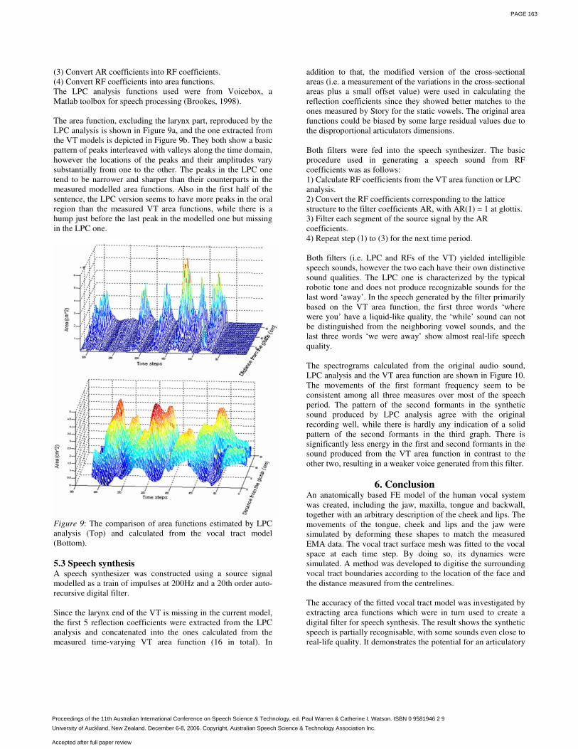
(3) Convert AR coefficients into RF coefficients. (4) Convert RF coefficients into area functions. The LPC analysis functions used were from Voicebox, a Matlab toolbox for speech processing (Brookes, 1998). The area function, excluding the larynx part, reproduced by the LPC analysis is shown in Figure 9a, and the one extracted from the VT models is depicted in Figure 9b. They both show a basic pattern of peaks interleaved with valleys along the time domain, however the locations of the peaks and their amplitudes vary substantially from one to the other. The peaks in the LPC one tend to be narrower and sharper than their counterparts in the measured modelled area functions. Also in the first half of the sentence, the LPC version seems to have more peaks in the oral region than the measured VT area functions, while there is a hump just before the last peak in the modelled one but missing in the LPC one.

Figure 9: The comparison of area functions estimated by LPC analysis (Top) and calculated from the vocal tract model (Bottom). 5.3 Speech synthesis A speech synthesizer was constructed using a source signal modelled as a train of impulses at 200Hz and a 20th order auto-recursive digital filter. Since the larynx end of the VT is missing in the current model, the first 5 reflection coefficients were extracted from the LPC analysis and concatenated into the ones calculated from the measured time-varying VT area function (16 in total). In

addition to that, the modified version of the cross-sectional areas (i.e. a measurement of the variations in the cross-sectional areas plus a small offset value) were used in calculating the reflection coefficients since they showed better matches to the ones measured by Story for the static vowels. The original area functions could be biased by some large residual values due to the disproportional articulators dimensions. Both filters were fed into the speech synthesizer. The basic procedure used in generating a speech sound from RF coefficients was as follows: 1) Calculate RF coefficients from the VT area function or LPC analysis. 2) Convert the RF coefficients corresponding to the lattice structure to the filter coefficients AR, with AR(1) = 1 at glottis. 3) Filter each segment of the source signal by the AR coefficients. 4) Repeat step (1) to (3) for the next time period. Both filters (i.e. LPC and RFs of the VT) yielded intelligible speech sounds, however the two each have their own distinctive sound qualities. The LPC one is characterized by the typical robotic tone and does not produce recognizable sounds for the last word ‘away’. In the speech generated by the filter primarily based on the VT area function, the first three words ‘where were you’ have a liquid-like quality, the ‘while’ sound can not be distinguished from the neighboring vowel sounds, and the last three words ‘we were away’ show almost real-life speech quality. The spectrograms calculated from the original audio sound, LPC analysis and the VT area function are shown in Figure 10. The movements of the first formant frequency seem to be consistent among all three measures over most of the speech period. The pattern of the second formants in the synthetic sound produced by LPC analysis agree with the original recording well, while there is hardly any indication of a solid pattern of the second formants in the third graph. There is significantly less energy in the first and second formants in the sound produced from the VT area function in contrast to the other two, resulting in a weaker voice generated from this filter.

6. Conclusion An anatomically based FE model of the human vocal system was created, including the jaw, maxilla, tongue and backwall, together with an arbitrary description of the cheek and lips. The movements of the tongue, cheek and lips and the jaw were simulated by deforming these shapes to match the measured EMA data. The vocal tract surface mesh was fitted to the vocal space at each time step. By doing so, its dynamics were simulated. A method was developed to digitise the surrounding vocal tract boundaries according to the location of the face and the distance measured from the centrelines. The accuracy of the fitted vocal tract model was investigated by extracting area functions which were in turn used to create a digital filter for speech synthesis. The result shows the synthetic speech is partially recognisable, with some sounds even close to real-life quality. It demonstrates the potential for an articulatory

Proceedings of the 11th Australian International Conference on Speech Science & Technology, ed. Paul Warren & Catherine I. Watson. ISBN 0 9581946 2 9

University of Auckland, New Zealand. December 6-8, 2006. Copyright, Australian Speech Science & Technology Association Inc.

Accepted after full paper review

PAGE 163

speech model to generate high quality human speech sounds, however some words were poorly synthesized. To further investigate the cause, LPC analysis was used to estimate the vocal tract area function from the original audio file. The comparison study indicates the possibilities of improperly scaling the articulators and incomplete articulatory movements.

Figure 10: (a) the spectrogram of the original speech signal (Wrench, 2001); (b) the spectrogram produced by the speech synthesized by LPC analysis; (c) the spectrogram of the speech synthesized by the vocal tract area function and the reflection coefficients from LPC analysis

7. Discussion

7.1 The issues associated with the VT area function The test shows that the digital filter based on the RF coefficients calculated from the original VT area functions does not produce intelligible sound. In fact, it hardly filtered the input signals. Its spectrogram indicated it did not redistribute enough acoustic energy into various formants to create distinctive vowel sounds. Looking at the Figures 7 and 9, we can find the area ratios between the adjacent sections do not vary as much as the ones either measured by Story or estimated by the LPC method. Each tract section seems to always carry a large residual area at any time instance during the speech. As a result, there are not large variations in the resulting RF coefficients which then lead to insufficient filtering on the input signal. On the other hand, the modified version of the area function, where the variation of the cross-sectional area was evaluated and re-offset by a much smaller residual area,

produces sharp filtered speech signal in contrast to the glottal input. This suggests that it is crucial to accurately measure the VT area functions in order to reproduce the intelligible speech sound. 7.2 The effect of the larynx in the speech synthesis Without the 5 reflection coefficients extracted from the LPC analysis, the filter can not yield intelligible speech sounds by using the measured area function alone. The presence of the larynx part of the area function is essential in determining the sound quality. During the speech synthesis, the larynx was assumed to be about a quarter of the total length of the vocal tract. There is always a large peak in the area function estimated by LPC, indicating major filtering property occurred in that region. Further investigation is required to explore the contribution to the voice from that part of the area function.

8. References Bier, P.J. (2003). Modelling the vocal tract. Unpublished

Master’s thesis. Bioengineering Institute, The University of Auckland.

Brookes, M. (1998). ‘VOICEBOX’ a free software for speech processing. Retrieved 09/09/2006 from http://www.ee.ic.ac.uk/hp/staff/dmb/voicebox/voicebox.html.

Essen, V.N., Erson, I.A., Hunter, P.J., Clarke, R.D. & Pullan, A.J. (2005). Anatomically based modelling of the human skull and jaw. Cells Tissues Organs ,180,44-53.

Fernandez, J., Mithraratne, P., Thripp, S., Tawhai, M., and Hunter, P. (2004). Anatomically based geometric modelling of the musculo-skeletal system and other organs. Biomechanics and Modelling in Mechanobiology, 2, 139-155.

Han, J.C. (2005). Modelling the human tongue. Unpublished 4th year project. Engineering Science department, the University of Auckland.

Mithraratne, P. (2006). Whole Organ Modelling course notes, The University of Auckland.

Story, B.H., Titze, I.R. & Hoffman, E.A. (1998). Vocal tract area functions for an adult female speaker based on volumetric imaging. J. Acoust. Soc. Am. 104(1), 471-487.

Wrench, A.A (2001). A multi-channel/multi-speaker articulatory database for continuous speech recognition research, Technical report. Department of Speech and Langage Sciences, Queen Margaret University College, United Kingdom.

Proceedings of the 11th Australian International Conference on Speech Science & Technology, ed. Paul Warren & Catherine I. Watson. ISBN 0 9581946 2 9

University of Auckland, New Zealand. December 6-8, 2006. Copyright, Australian Speech Science & Technology Association Inc.

Accepted after full paper review

PAGE 164