A tutorial on the piecewise regression approach applied to bedload

United StatesDepartmentof Agriculture

Forest Service General Technical Report RMRS-GTR-189Rocky Mountain Research Station May 2007

A Tutorial on the Piecewise Regression Approach Applied to

Bedload Transport Data

Sandra E. RyanLaurie S. Porth

Ryan, Sandra E.; Porth, Laurie S. 2007. A tutorial on the piecewise regression ap-proach applied to bedload transport data. Gen. Tech. Rep. RMRS-GTR-189. Fort Collins, CO: U.S. Department of Agriculture, Forest Service, Rocky Mountain Research Station. 41 p.

Abstract

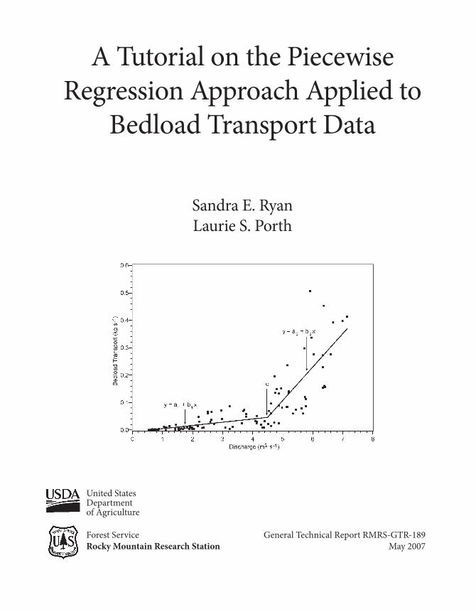
This tutorial demonstrates the application of piecewise regression to bedload data to define a shift in phase of transport so that the reader may perform similar analyses on available data. The use of piecewise regression analysis implicitly recognizes dif-ferent functions fit to bedload data over varying ranges of flow. The transition from primarily low rates of sand transport (Phase I) to higher rates of sand and coarse gravel transport (Phase II) is termed “breakpoint” and is defined as the flow where the fitted functions intersect. The form of the model used here fits linear segments to different ranges of data, though other types of functions may be used. Identifying the transition in phases is one approach used for defining flow regimes that are essen-tial for self-maintenance of alluvial gravel bed channels. First, the statistical theory behind piecewise regression analysis and its procedural approaches are presented. The reader is then guided through an example procedure and the code for generating an analysis in SAS is outlined. The results from piecewise regression analysis from a number of additional bedload datasets are presented to help the reader understand the range of estimated values and confidence limits on the breakpoint that the anal-ysis provides. The identification and resolution of problems encountered in bedload datasets are also discussed. Finally, recommendations on a minimal number of sam-ples required for the analysis are proposed.

Keywords: Piecewise linear regression, breakpoint, bedload transport

You may order additional copies of this publication by sending your mailing information in label form through one of the following media. Please specify the publication title and series number.

Publishing Services

Telephone (970) 498-1392 FAX (970) 498-1122 E-mail [email protected] Web site http://www.fs.fed.us/rm/publications Mailing address Publications Distribution

Rocky Mountain Research Station 240 West Prospect Road Fort Collins, CO 80526

Rocky Mountain Research StationNatural Resources Research Center

2150 Centre Avenue, Building AFort Collins, CO 80526

Authors

Sandra E. Ryan, Research Hydrologist/GeomorphologistU.S. Forest Service

Rocky Mountain Research Station240 West Prospect RoadFort Collins, CO 80526

E-mail: [email protected]: 970-498-1015

Fax: 970-498-1212

Laurie S. Porth, StatisticianU.S. Forest Service

Rocky Mountain Research Station240 West Prospect RoadFort Collins, CO 80526E-mail: [email protected]: 970-498-1206

Fax: 970-498-1212

Statistical code and output shown in boxed text in the document (piecewise regression procedure and bootstrapping), as well as an electronic version of the Little Granite Creek dataset are available on the Stream System Technology Center website under“software” at http://stream.fs.fed.us/publications/software.html.

Contents

Introduction .................................................................................... 1

Data ................................................................................................. 2

Statistical Theory........................................................................... 2

Tutorial Examples .......................................................................... 4Little Granite Creek Example ................................................... 4Hayden Creek Example ......................................................... 18

Potential Outliers ......................................................................... 28

Guidelines .................................................................................... 30

Summary ...................................................................................... 35

References ................................................................................... 36

Appendix A—Little Granite Creek example dataset .................... 38

Appendix B—Piecewise regression results with bootstrap confidence intervals ............................................................... 40

ii

USDA Forest Service RMRS-GTR-189. 2007 1

Introduction

Bedload transport in coarse-bedded streams is an irregular process influenced by a number of factors, including spatial and temporal variability in coarse sediment available for transport. Variations in measured bedload have been attributed to fluctuations occurring over several scales, including individual particle movement (Bunte 2004), the passing of bedforms (Gomez and others 1989, 1990), the presence of bedload sheets (Whiting and others 1988), and larger pulses or waves of stored sediment (Reid and Frostick 1986). As a result, rates of bedload transport can exhibit exceptionally high variability, often up to an order of magnitude or greater for a given discharge. However, when rates of transport are assessed for a wide range of flows, there are relatively predictable patterns in many equilibrium gravel-bed channels.

Coarse sediment transport has been described as occurring in phases, where there are distinctly different sedimentological characteristics associated with flows under different phases of transport. At least two phases of bedload transport have been described (Emmett 1976). Under Phase I transport, rates are relatively low and consist primarily of sand and a few small gravel particles that are considerably finer than most of the material comprising the channel bed. Phase I likely represents re-mobilization of fine sediment deposited from previous transport events in pools and tranquil areas of the bed (Paola and Seal 1995, Lisle 1995). Phase II transport represents initiation and transport of grains from the coarse surface layer common in steep mountain channels, and consists of sand, gravel, and some cobbles moved over a stable or semi-mobile bed. The beginning of Phase II is thought to occur at or near the “bankfull” discharge (Parker 1979; Parker and others 1982; Jackson and Beschta 1982; Andrews 1984; Andrews and Nankervis 1995), but the threshold is often poorly or subjectively defined.

Ryan and others (2002, 2005) evaluated the application of a piecewise regression model for objectively defining phases of bedload transport and the discharge at which there is a substantial change in the nature of sediment transport in gravel bed streams. The analysis recognizes the existence of different transport relationships for different ranges of flow. The form of the model used in these evaluations fit linear segments to the ranges of flow, though other types of functions may be used. A breakpoint was defined by the flow where the fitted functions intersected. This was interpreted as the transition between phases of transport. Typically, there were markedly different statis-tical and sedimentological features associated with flows that were less than or greater than the breakpoint discharge. The fitted line for less-than-breakpoint flows had a lower slope with less variance due to the fact that bedload at these discharges consisted primarily of small quantities of sand-sized materials. In

2 USDA Forest Service RMRS-GTR-189. 2007

contrast, the fitted line for flows greater than the breakpoint had a significantly steeper slope and more variability in transport rates due to the physical breakup of the armor layer, the availability of subsurface material, and subsequent changes in both the size and volume of sediment in transport.

Defining the breakpoint or shift from Phase I to Phase II using measured rates of bedload transport comprises one approach for defining flow regimes essential for self-maintenance of alluvial gravel bed channels (see Schmidt and Potyondy 2004 for full description of channel maintenance approach). The goal of this tutorial is to demonstrate the application of piecewise regression to bedload data so that the reader may perform similar analyses on available data. First we present statistical theory behind piecewise regression and its procedural approaches. We guide the reader through an example procedure and provide the code for generating an analysis using SAS (2004), which is a statis-tical analysis software package. We then present the results from a number of examples using additional bedload datasets to give the reader an understanding of the range of estimated values and confidence limits on the breakpoint that this analysis provides. Finally, we discuss recommendations on minimal number of samples required, and the identification and resolution of problems encoun-tered in bedload datasets.

Data

Data on bedload transport and discharge used in this application were obtained through a number of field studies conducted on small to medium sized gravel-bedded rivers in Colorado and Wyoming. The characteristics of channels from which the data originate and the methods for collecting the data are fully described in Ryan and others (2002, 2005). Flow and rate of bedload transport are the primary variables used in the assessment of the breakpoint. Bedload was collected using hand-held bedload samplers, either while wading or, more typically, from sampling platforms constructed at the channel cross-sections. Mean flow during the period of sample collection was obtained from a nearby gaging station or from flow rating curves established for the sites.

Statistical Theory

When analyzing a relationship between a response, y, and an explanatory variable, x, it may be apparent that for different ranges of x, different linear rela-tionships occur. In these cases, a single linear model may not provide an adequate description and a nonlinear model may not be appropriate either. Piecewise linear regression is a form of regression that allows multiple linear models to be


fit to the data for different ranges of x. Breakpoints are the values of x where the slope of the linear function changes (fig. 1). The value of the breakpoint may or may not be known before the analysis, but typically it is unknown and must be estimated. The regression function at the breakpoint may be discontinuous, but a model can be written in such a way that the function is continuous at all points including the breakpoints. Given what is understood about the nature of bedload transport, we assume the function should be continuous. When there is only one breakpoint, at x=c, the model can be written as follows: y = a

1 + b

1x forx≤c

y = a2 + b

2x forx>c.

In order for the regression function to be continuous at the breakpoint, the two equations for y need to be equal at the breakpoint (when x = c):

a1 + b

1c=a

2 + b

2c.

Solve for one of the parameters in terms of the others by rearranging the equation above:

a2 = a

1+c(b

1 - b

2).

Then by replacing a2 with the equation above, the result is a piecewise regres-

sion model that is continuous at x=c:

y = a1 + b

1x forx≤c

y = {a1+c(b

1 - b

2)} + b

2x forx>c.

Nonlinear least squares regression techniques, such as PROC NLIN in SAS, can be used to fit this model to the data.

Figure 1—Example of a piecewise regression fit between discharge and bedload transport data collected at St. Louis Creek Site 2, Fraser Experimental Forest (Ryan and others 2002).


Tutorial Examples

In order to run the examples from these tutorials the user must have some knowledge of SAS, such as the ability to move around in the SAS environment and import data. SAS version 9.1.3 was used to implement these programs. Most of this code will work with SAS versions beginning with 8.2, but it is important to note that the nonlinear regression procedure used to fit the models was modified between versions 8.2 and 9, and this can produce slight differ-ences in the final results.

Little Granite Creek Example

Data from Little Granite Creek near Jackson, Wyoming were collected by William Emmett and staff from the U.S. Geological Survey from 1982 through 1992. Sandra Ryan of the U.S. Forest Service, Rocky Mountain Research Station collected additional data during high runoff in 1997. This dataset has over 120 observations from a wide range of flows (Appendix A) (Ryan and Emmett 2002).

Estimating starting parametersThe first step in applying piecewise regression to bedload and flow data is

to graph the data and estimate where the breaks appear to occur. Applying a nonparametric smooth to the data, such as a LOESS fit (box 1), can help the user determine where these breaks manifest themselves. Using figure 2, we visually estimate the breakpoint to be somewhere between 4.0 and 8.0 m3 s-1.

Box 1. Apply a nonparametric smooth to the data and generate figure 2.

* -- USE LOESS PROCEDURE TO GET SMOOTHED NONPARAMETRIC FIT OF DATA -- *;PROC LOESS DATA=ltlgran; MODEL Y=X; ODS OUTPUT OUTPUTSTATISTICS=LOESSFIT;RUN;* -- PLOT DATA AND THE LOESS FIT -- *;SYMBOL1 f=marker v=U i=none c=black;SYMBOL2 v=none i=join line=1 w=3 c=black;AXIS2 label = (a=90 r=0);PROC GPLOT DATA=LOESSFIT; PLOT DEPVAR*X=1 PRED*X=2 / OVERLAY FRAME VAXIS=AXIS2;RUN;

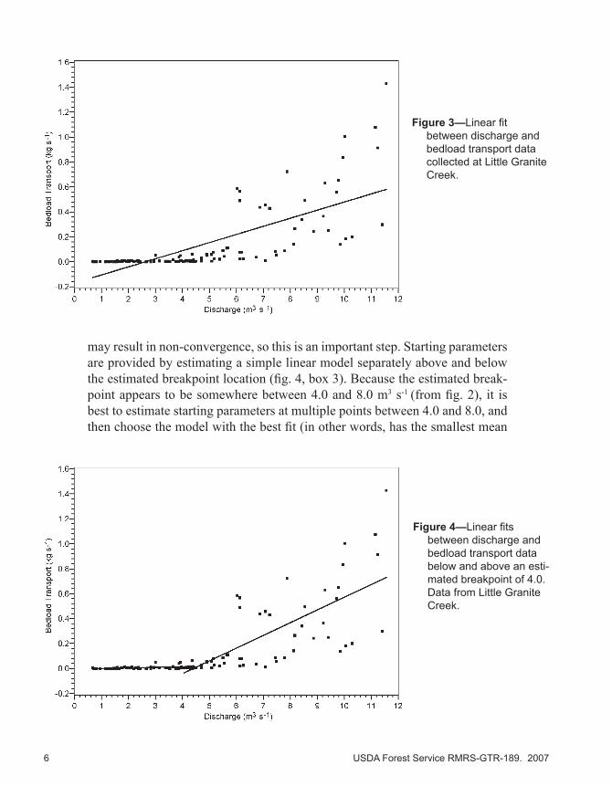
A standard linear regression model is then fit to the entire data range (fig. 3, box 2). It is apparent the linear model is a poor fit over the entire range of discharges because the values obtained at lower flows do not fall along the line. The results from this model (box 2) will be used as a baseline to compare with the piecewise model. To be acceptable, the piecewise model should account for more variability than the linear model.


Box 2. Apply a linear regression model to the data and generate figure 3.

* -- APPLY LINEAR REGRESSION MODEL TO THE DATA -- *;PROC REG DATA=ltlgran; MODEL Y=X; OUTPUT OUT=LINEARFIT P=PRED;RUN;* -- PLOT DATA AND THE LINEAR REGRESSION FIT -- *;SYMBOL1 f=marker v=U i=none c=black;SYMBOL2 v=none i=join line=1 w=3 c=black;AXIS2 label = (a=90 r=0);PROC GPLOT DATA=LINEARFIT; PLOT Y*X=1 PRED*X=2 / OVERLAY FRAME VAXIS=AXIS2;RUN;

Analysis of Variance – Linear Model Sum of Mean Source DF Squares Square F Value Pr > F Model 1 4.25406 4.25406 138.95 <.0001 Error 121 3.70441 0.03061 Corrected Total 122 7.95847

Root MSE 0.17497 R-Square 0.5345 Dependent Mean 0.12540 Adj R-Sq 0.5307 Coeff Var 139.53045

Starting parameters (a1, b

1, b

2,c) are needed in the PROC NLIN procedure

to give the program a place to begin fitting the model. Poor starting parameters

Figure 2—Loess fit between discharge and bedload transport data collected at Little Granite Creek.


may result in non-convergence, so this is an important step. Starting parameters are provided by estimating a simple linear model separately above and below the estimated breakpoint location (fig. 4, box 3). Because the estimated break-point appears to be somewhere between 4.0 and 8.0 m3 s-1 (from fig. 2), it is best to estimate starting parameters at multiple points between 4.0 and 8.0, and then choose the model with the best fit (in other words, has the smallest mean

Figure 4—Linear fits between discharge and bedload transport data below and above an esti-mated breakpoint of 4.0. Data from Little Granite Creek.

Figure 3—Linear fit between discharge and bedload transport data collected at Little Granite Creek.


squared error). We obtained initial starting parameters for models where the breakpoint was 4.0, 6.0 (half-way), and 8.0.

Box 3. Apply two linear regression models to the data and generate figure 4.

* -- APPLY LINEAR REG MODEL TO DATA BELOW ESTIMATED BREAKPOINT -- *;PROC REG DATA=ltlgran; MODEL Y=X; OUTPUT OUT=FITBELOW P=PREDBELOW; WHERE X <= 4.0;RUN;* -- APPLY LINEAR REG MODEL TO DATA ABOVE ESTIMATED BREAKPOINT -- *;PROC REG DATA=ltlgran; MODEL Y=X; OUTPUT OUT=FITABOVE P=PREDABOVE; WHERE X > 4.0;RUN;* -- COMBINE DATASETS -- *;DATA FITBOTH; SET FITBELOW FITABOVE;RUN;* -- PLOT DATA AND THE TWO LINEAR REGRESSION FITS -- *;SYMBOL1 f=marker v=U i=none c=black;SYMBOL2 v=none i=join line=1 w=3 c=black;AXIS2 label = (a=90 r=0);PROC GPLOT DATA=FITBOTH; PLOT Y*X=1 PREDBELOW*X=2 PREDABOVE*X=2 / OVERLAY FRAME VAXIS=AXIS2;RUN;

Linear Fit Below Estimated Breakpoint=4.0

Parameter Standard Variable Label DF Estimate Error t Value Pr > |t| Intercept Intercept 1 -0.00422 0.00307 -1.37 0.1749 X Discharge (cubic meters/sec) 1 0.00473 0.00128 3.70 0.0005

Linear Fit At and Above Estimated Breakpoint=4.0

Parameter Standard Variable Label DF Estimate Error t Value Pr > |t| Intercept Intercept 1 -0.45074 0.08280 -5.44 <.0001 X Discharge (cubic meters/sec) 1 0.10221 0.01174 8.71 <.0001

The estimated starting parameters for the piecewise model,

y = a1 + b

1x forx≤c

y = {a1+c(b

1 - b

2)} + b

2x forx>c.

and the methods used to obtain them are shown in table 1.


Fitting the modelThe starting parameters are then used to fit the piecewise regression model

with PROC NLIN procedure in SAS (fig. 5, box 4).

Table 1—Estimated piecewise regression starting parameters for a breakpoint at 4.0.

Estimated starting Parameter parameter How obtained

a1 -0.00422 Intercept of linear fit to data below estimated breakpoint.

b1 0.00473 Slope of linear fit to data below estimated breakpoint.

b2 0.10221 Slope of linear fit to data above estimated breakpoint.

c 4.0 Estimated breakpoint from LOESS plot.

Figure 5—Piecewise regression between discharge and bedload transport data collected at Little Granite Creek. A power function is shown for comparison.


Box 4. Apply a piecewise and power model to the data and generate figure 5.

* -- FIT THE PIECEWISE MODEL USING NONLINEAR PROCEDURE -- *;PROC NLIN DATA=ltlgran MAXITER=1000 METHOD=MARQUARDT; PARMS a1=-0.00422 b1=0.00473 c=4 b2=0.10221; Xpart = a1 + b1*X; IF (X > c) THEN DO; Xpart = a1 + c*(b1-b2) + b2*X; end; MODEL Y = Xpart; OUTPUT OUT=PIECEFIT R=RESID P=PRED;RUN;* -- FIT THE POWER MODEL (FOR COMPARISON) USING NONLINEAR PROCEDURE -- *;PROC NLIN DATA=ltlgran MAXITER=1000 METHOD=MARQUARDT; PARMS a1=0.01 b1=0.01 b2=1.0; MODEL Y = a1 + b1*X**b2; OUTPUT OUT=POWERFIT R=PWR_RESID P=PWR_PRED;RUN;* -- COMBINE OUTPUT FROM BOTH MODELS -- *;DATA ALL; SET PIECEFIT POWERFIT;RUN; * -- PLOT DATA, PIECEWISE REGRESSION FIT, AND POWER MODEL FIT -- *;SYMBOL1 f=marker v=U i=none c=black;SYMBOL2 v=none i=join line=1 w=3 c=black;SYMBOL3 v=none i=join line=2 w=3 c=black;AXIS2 label = (a=90 r=0);PROC GPLOT DATA=ALL; PLOT Y*X=1 PRED*X=2 PWR_PRED*X=3 / OVERLAY FRAME VAXIS=AXIS2;RUN;

Little Granite CreekPiecewise Regression Fit

The NLIN ProcedureDependent Variable Y

Method: MarquardtIterative Phase

Sum of Iter a1 b1 c b2 Squares 0 -0.0150 0.00949 6.0000 0.1081 3.2790 1 -0.0150 0.00949 4.9368 0.1081 2.8875 2 -0.00484 0.00485 4.9114 0.1104 2.8825 3 -0.00377 0.00432 4.8794 0.1100 2.8822 4 -0.00223 0.00355 4.8340 0.1094 2.8820 5 -0.00223 0.00355 4.8341 0.1094 2.8820 NOTE: Convergence criterion met. Sum of Mean Approx Source DF Squares Square F Value Pr > F Model 3 5.0765 1.6922 69.87 <.0001 Error 119 2.8820 0.0242 Corrected Total 122 7.9585 Approx Parameter Estimate Std Error Approximate 95% Confidence Limits a1 -0.00223 0.0423 -0.0860 0.0815 b1 0.00355 0.0141 -0.0244 0.0315 c 4.8341 0.4977 3.8486 5.8197 b2 0.1094 0.0115 0.0867 0.1320


Under the “Iterative Phase” of the output, there is a note indicating “Convergence criterion met.” This means the model converged and a break-point of 4.83 and a mean squared error (MSE) of 0.0242 were estimated. If we repeat the above series of steps for breakpoints at 6.0 and 8.0, we get models that converge with breakpoints at 4.83 (with MSE=0.0242), which is the same model produced with an initial breakpoint of 4.0, and 8.27 (with MSE=0.0246), respectively. The models that converged with a breakpoint of 4.83 have the smallest MSE and therefore the best fit.

The results from the piecewise regression model are then compared with those from the linear model (fig. 3). An extra sums of squares test (Neter and others 1990) can be used to determine if the piecewise regression model is an improvement over the linear model. Other models can also be compared, such as a power model (also shown in fig. 5) commonly used in fitting bedload data (Whiting and others 1999). However, there is no formal test available that allows the direct comparison of a piecewise regression model to a power model, but one can compare the results using the model standard error, also known as the square root of the mean squared error. This is the average distance of each observation from the fitted model and smaller values indicate an improved fit. The results from curve fits to the Little Granite Creek data are compared in table 2.

Table 2—Model standard errors for the linear, power, and piecewise regression models for Little Granite Creek.

Least squares model Model standard error

Linear: y = a1 + b

1x 0.0306

Power: y = a1 + b

1xb2 0.0230

Piecewise 0.0242

Based on comparisons of the model standard error and the visual fit, the linear model is clearly not the best fit. However, the model standard error for the piecewise linear model isn’t substantially different from the power model. Justification for using the piecewise regression model in this case would be based on scientific reasons (Bates and Watts 1988). That is, if the piecewise regression model has approximately the same goodness of fit as a different model, then scientific reasoning could be used to select the model. In this case, we choose the piecewise model to objectively determine the onset of different phases of bedload transport that have been shown to exist in many gravel bed rivers.

Testing model assumptionsThe next step is to ensure that the assumptions of the model have been met.

The first assumption in regression analysis is the independence of the residuals


(which are the actual-y minus predicted-y values), meaning the value of one residual is unrelated to the value of the next. As an example of dependence, bedload samples are often taken in the field over relatively short time intervals (hours to days), causing potential correlation between discharge values due to time. If the values of x are correlated, then the residuals will be correlated. Neter and others (1990) state that if the data are correlated, the regression coefficients are still unbiased but may be inefficient, and the mean squared error and standard deviations of the parameters may be seriously underesti-mated. A plot of the residuals over time should show no trends, otherwise the assumed independence of the x values is violated. The Little Granite Creek dataset contains data ranging from April through July for 1985 through 1997. It is difficult to show trends on a single plot for such a lengthy period of record, so for simplicity we plot the data sequentially assuming equal distance between the measurements (box 5).

Box 5. Check residuals for independence by generating figure 6.

* -- SORT THE DATA BY TIME -- *;PROC SORT DATA=PIECEFIT; BY date;RUN;* -- ADD A DUMMY TIME VARIABLE TO MAKE PLOTTING EASIER -- *;DATA PIECEFIT; RETAIN TIME 0; SET PIECEFIT; TIME = TIME + 1;RUN;* -- PLOT THE RESIDUALS OVER TIME IN ORDER TO CHECK FOR INDEPENDENCE -- *;SYMBOL1 f=marker v=U i=join c=black;AXIS2 label = (a=90 r=0);PROC GPLOT DATA=PIECEFIT; PLOT X*TIME=1 / FRAME VAXIS=AXIS2;RUN;

From the graph of the residuals over time (fig. 6), it is apparent there may be some correlation because the residuals are not randomly scattered above and below zero. For instance, around time 100 there are nine consecutive data points below zero and then eleven consecutive data points above zero. One way to check for correlation is to model the residuals using an autoregressive [AR(1)] variance structure, which takes into account that a particular observa-tion is correlated with the previous observation (box 6). In other words, we can better predict the value of the current observation if we use the value of the previous observation. If there is a substantial difference between this adjusted MSE (which is the valid MSE for the model) and the MSE from the original piecewise regression model, then the implication is that the residuals are corre-lated. Setting SUBJECT=year tells SAS there is no correlation between years.


The data for this particular site represent approximately April through July of each year and we would not expect the July measurement to be correlated with April measurement of the following year. Assuming only the correlation within each year, the estimate for the correlation parameter is 0.6194 (box 6), and the Wald Z-test shows a significant p-value (p<0.0001). This means the residuals are significantly correlated, and the MSE is actually 0.0226. The MSE from the piecewise regression model was 0.0242, which is only a 7 percent difference so we assume the effects of correlation are not substantial.

Box 6. Apply an autoregressive model to the residuals.

*-- SORT THE DATA BY TIME -- *;PROC SORT DATA=PIECEFIT; BY date;RUN;* -- MODEL THE RESIDUALS AS AN AR(1) -- *; PROC MIXED DATA=PIECEFIT; MODEL RESID=; REPEATED / SUBJECT=year TYPE=AR(1);RUN;

Little Granite CreekGET MSE ADJUSTED FOR CORRELATION

Convergence criteria met. Covariance Parameter Estimates

Standard Z Cov Parm Subject Estimate Error Value Pr Z Alpha Lower Upper AR(1) YEAR 0.6194 0.06630 9.34 <.0001 0.05 0.4895 0.7493 Residual 0.02256 0.004031 5.60 <.0001 0.05 0.01635 0.03313

Figure 6—Piecewise regres-sion residuals for Little Granite Creek plotted sequentially to check for independence.


A second assumption is that the residuals exhibit normality. This means the error in the model prediction, which is the distribution of the residuals, should appear to be a bell-shaped curve (a normal distribution) with many “average” sized residuals and fewer large and small residuals. Too many extreme values, small or large, suggest a skewed distribution. A visual way to determine if the residuals follow the normal distribution is to generate a QQ-plot, which is a graph of the quantiles of the normal distribution against the quantiles of the data (box 7). If the data closely match the quantiles of the normal distribution, then the data are normal. With a piecewise regression model, which consists of two linear models, we examine the residuals below and then above the break-point (fig. 7).

Box 7. Check residuals for normality and generate figure 7.

* -- CHECK RESIDUALS FOR NORMALITY BELOW THE BREAKPOINT -- *;SYMBOL1 f=marker v=U i=none c=black;PROC UNIVARIATE DATA=PIECEFIT NORMAL; WHERE (X <= 4.83); VAR RESID; QQPLOT RESID / NORMAL(MU=EST SIGMA=EST);RUN;* -- CHECK RESIDUALS FOR NORMALITY ABOVE THE BREAKPOINT -- *;PROC UNIVARIATE DATA=PIECEFIT NORMAL; WHERE (X > 4.83); VAR RESID; QQPLOT RESID / NORMAL(MU=EST SIGMA=EST);RUN;

Tests for NormalityChecking for Normality Below the Breakpoint

Test -------Statistic-------- -----------p Value----------- Shapiro-Wilk W 0.659789 Pr < W <0.0001 Kolmogorov-Smirnov D 0.24104 Pr > D <0.0100 Cramer-von Mises W-Sq 1.268588 Pr > W-Sq <0.0050 Anderson-Darling A-Sq 7.403709 Pr > A-Sq <0.0050

Tests for NormalityChecking for Normality Above the Breakpoint

Test --------Statistic------- -----------p Value----------- Shapiro-Wilk W 0.970409 Pr < W 0.2869 Kolmogorov-Smirnov D 0.113803 Pr > D 0.1387 Cramer-von Mises W-Sq 0.068001 Pr > W-Sq >0.2500 Anderson-Darling A-Sq 0.424133 Pr > A-Sq >0.2500

The visual interpretation of the two plots suggests that the residuals of the data below the breakpoint (fig. 7a) are not normal, while the data above the breakpoint (fig. 7b) exhibit a near one-to-one relationship between the data and the normal distribution. Another way to check for normality is to use the Shapiro-Wilk test (among others in box 7). The results from this test show that the residuals below the breakpoint are, indeed, not normal (p<0.0001), but we cannot reject normality for the residuals above the breakpoint (p=0.2869).


A third assumption is that residuals have homogeneous variance, with the variability of the residuals between and within the fitted segments being approx-imately constant. By plotting the residuals on the y-axis and the predicted fit on the x-axis, one can determine if the variability of the data is constant across the entire range of x (fig. 8, box 8). The linearity assumption, where an equal number of data points randomly occur on either side of the model, can also be

Figure 7—QQ-plots for Little Granite Creek piecewise regression residuals for curves fit to data (a) below and (b) above the break-point value.


examined using the plot of the residuals versus the predicted values. Figure 8(a and b) shows nearly half the data points are below and half above the line. Hence, the linearity of the two segments is not in question. However, it is apparent the residuals are not homogeneous because the variance increases with the predicted value. The reader is referred to Neter and others (1990) for additional explanation of the assumptions of a regression model.

Figure 8—Little Granite Creek piecewise regres-sion residuals and predicted values (a) below and (b) above the breakpoint.


Box 8. Check residuals for lack of fit and heterogeneous variance and generate figure 8.

* -- CHECK RESIDS FOR LACK OF FIT & HETEROGENOUS VARIANCE BELOW BREAKPOINT-- *;SYMBOL1 f=marker v=U i=none c=black;AXIS2 label = (a=90 r=0);PROC GPLOT DATA=PIECEFIT; WHERE (X <= 4.83); PLOT RESID*PRED=1 / frame VAXIS=AXIS2 VREF=0;RUN;* -- CHECK RESIDS FOR LACK OF FIT & HETEROGENOUS VARIANCE ABOVE BREAKPOINT-- *;PROC GPLOT DATA=PIECEFIT; WHERE (X > 4.83); PLOT RESID*PRED=1 / FRAME VAXIS=AXIS2 VREF=0;RUN;

Implications of assumption violationsWhen the residuals are not independent, then a time series analysis may be

more appropriate for predicting changes in transport rate over time. When the linearity assumption is violated, then a linear model is not the best fit for the data. Violations of the normality and/or homogeneous variance assumptions result in unreliable estimates of the standard error and confidence intervals for the model parameters, but the parameter estimates themselves are unbiased (Neter and others 1990). A nonparametric method, such as bootstrapping, can be used to estimate the accuracy in the estimation of a parameter (Efron and Tibshirani 1993). Bootstrapping involves resampling from the original dataset, with replacement, in order to obtain a secondary dataset. The piecewise model is then fit to the secondary datasets and the parameter estimates (a

1, b

1, b

2,c)

are retained. Using the parameter estimates from secondary datasets generated in these analysis (n=2000), nonparametric standard errors and confidence intervals can be estimated for the original piecewise regression model. If the data exhibit violations of the normality and variance assumptions as well as the independence assumption, it is up to the user to determine if they would prefer to use a time series approach to the analysis or address primarily the normality and variance issues, and realize possible bias of the MSE due to the correlation issue.

For the Little Granite Creek data, the MSE from the autoregressive model applied to the residuals did not differ substantially from the original model MSE, so we chose to ignore the modest correlation effect and focus on the lack of normality and homogeneous variance problems. Bootstrapping techniques were used to obtain confidence intervals and standard errors for the piecewise regression model (table 3). The analysis estimates the breakpoint as 4.8 m3 s-1 with 95 percent confidence interval ranging from 3.97 to 8.00 m3 s-1, which is a fairly sizable range (fig. 9, table 3). Sampling more data points at flows near


the breakpoint value might improve the fit and confidence of the estimates. It is also important to note that this is where the variance in the data starts to rapidly increase, which also contributes to wider confidence bands. A discharge of 4.8 m3 s-1 is about 81 percent of the bankfull discharge determined for this site (Q

1.5 = 5.95 m3 s-1). Ryan and others (2002, 2005) have shown that the break-

point occurs at about 80 percent of the bankfull discharge in many gravel bed channels measured in Colorado and Wyoming. The confidence bands on this estimate are typically between 60 and 100 percent of the bankfull discharge.

Table 3—Little Granite Creek piecewise regression parameter values with corresponding bootstrap estimates of the standard error and 95 percent confidence intervals.

Bootstrap 95% BCaa Confidence intervals Parameter Estimate standard error (lower, upper)

a1 -0.00223 0.01174 -0.04413 0.00076

b1 0.00355 0.00497 0.00177 0.02104

b2 0.10936 0.07082 0.07064 0.25879

c 4.83411 0.94901 3.96558 8.00188

aBCa confidence intervals are considered the better bootstrap intervals because they are bettered bias-corrected and accelerated confidence intervals (Efron and Tibshirani 1993).

Figure 9—Piecewise regres-sion fit between discharge and bedload transport data collected at Little Granite Creek with error bars denoting width of 95 percent confidence intervals for the estimated breakpoint.


Hayden Creek Example

Data from Hayden Creek near Salida, CO was collected by staff from the USFS Rocky Mountain Research Station and the Pike/San Isabel National Forest during snowmelt runoff in 1998 and 1999. This dataset has very few observations collected at higher flows, making the piecewise regression model fitting more challenging and the interpretations more difficult. Repeating the series of steps outlined for Little Granite Creek, the data for Hayden Creek are first plotted with the nonparameteric LOESS fit to estimate the value of the breakpoint (box 9). The breakpoint is visually estimated to be somewhere between 1.3 m3 s-1 and 1.7 m3 s-1 (fig. 10).

Box 9. Apply a nonparametric smooth to the data and generate figure 10.

* -- USE LOESS PROCEDURE TO GET SMOOTHED NONPARAMETRIC FIT OF DATA -- *;PROC LOESS DATA=hayden; MODEL Y=X; ODS OUTPUT OUTPUTSTATISTICS=LOESSFIT;RUN;* -- PLOT DATA AND THE LOESS FIT -- *;SYMBOL1 f=marker v=U i=none c=black;SYMBOL2 v=none i=join line=1 c=black;AXIS2 label = (a=90 r=0);PROC GPLOT DATA=LOESSFIT; PLOT DEPVAR*X=1 PRED*X=2 / OVERLAY FRAME VAXIS=AXIS2;RUN;

Figure 10—Loess fit between discharge and bedload transport data collected at Hayden Creek.


Next, a standard linear regression model is fit to the entire data range (fig. 11, box 10). It appears there may be a better model than the linear fit for this data.

Box 10. Apply a linear regression model to the data and generate figure 11.

* -- APPLY LINEAR REGRESSION MODEL TO THE DATA -- *;PROC REG DATA=hayden; MODEL Y=X; OUTPUT OUT=LINEARFIT P=PRED;RUN;* -- PLOT DATA AND THE LINEAR REGRESSION FIT -- *;SYMBOL1 f=marker v=U i=none c=black;SYMBOL2 v=none i=join line=1 c=black;AXIS2 label = (a=90 r=0);PROC GPLOT DATA=LINEARFIT; PLOT Y*X=1 PRED*X=2 / OVERLAY FRAME VAXIS=AXIS2;RUN;

Analysis of Variance Sum of Mean Source DF Squares Square F Value Pr > F Model 1 0.00627 0.00627 110.95 <.0001 Error 74 0.00418 0.00005653 Corrected Total 75 0.01046 Root MSE 0.00752 R-Square 0.5999 Dependent Mean 0.01097 Adj R-Sq 0.5945 Coeff Var 68.52498

Figure 11—Linear fit between discharge and bedload transport data collected at Hayden Creek.


With an estimated breakpoint between 1.3 and 1.7 m3 s-1, the initial starting parameters are obtained for models where the breakpoint was 1.3, 1.5 (half-way), and 1.7. The following code is used to obtain starting parameters estimates for a breakpoint at 1.5 (fig. 12, box 11). The estimated parameters used in the analysis are shown table 4.

Box 11. Apply two linear regression models to the data and generate figure 12.

* -- APPLY LINEAR REG MODEL TO DATA BELOW ESTIMATED BREAKPOINT -- *;PROC REG DATA=hayden; MODEL Y=X; OUTPUT OUT=FITBELOW P=PREDBELOW; WHERE X <= 1.5;RUN;* -- APPLY LINEAR REG MODEL TO DATA ABOVE ESTIMATED BREAKPOINT -- *;PROC REG DATA=hayden; MODEL Y=X; OUTPUT OUT=FITABOVE P=PREDABOVE; WHERE X > 1.5;RUN;* -- COMBINE DATASETS -- *;DATA FITBOTH; SET FITBELOW FITABOVE;RUN;* -- PLOT DATA AND THE TWO LINEAR REGRESSION FITS -- *;SYMBOL1 f=marker v=U i=none c=black;SYMBOL2 v=none i=join line=1 c=black;AXIS2 label = (a=90 r=0);PROC GPLOT DATA=FITBOTH; PLOT Y*X=1 PREDBELOW*X=2 PREDABOVE*X=2 / OVERLAY FRAME VAXIS=AXIS2;RUN;

Linear Fit Below Estimated Breakpoint=1.5 Parameter Standard Variable Label DF Estimate Error t Value Pr > |t| Intercept Intercept 1 -0.00675 0.00137 -4.92 <.0001 X Discharge (cubic meters/sec) 1 0.01435 0.00136 10.57 <.0001

Linear Fit At and Above Estimated Breakpoint=1.5 Parameter Standard Variable Label DF Estimate Error t Value Pr > |t| Intercept Intercept 1 -0.11531 0.02823 -4.09 0.0010 X Discharge (cubic meters/sec) 1 0.08285 0.01663 4.98 0.0002

Using these parameters, the piecewise regression model is fit with PROC NLIN procedure (fig. 13, box 12).


Figure 12—Two estimates of linear fits between discharge and bedload transport below and above an estimated breakpoint of 1.5. Data are from Hayden Creek.

Table 4—Estimated piecewise regression starting parameters for Hayden Creek with an estimated breakpoint at 1.5.

Estimated Parameter starting parameter How obtained

a1 -0.00675 Intercept of linear fit to data below estimated breakpoint.

b1 0.01435 Slope of linear fit to data below estimated breakpoint.

b2 0.08285 Slope of linear fit to data above estimated breakpoint.

c 1.5 Estimated breakpoint from LOESS plot.

Figure 13—Piecewise regression and power fit between discharge and bedload transport data collected at Hayden Creek.


Box 12. Apply a piecewise and power model to the data and generate figure 13.

* -- FIT THE PIECEWISE MODEL USING NONLINEAR PROCEDURE -- *;PROC NLIN DATA=hayden MAXITER=1000 METHOD=MARQUARDT; PARMS a1=-0.00675 b1=0.01435 c=1.5 b2=0.08285; Xpart = a1 + b1*X; IF (X > c) THEN DO; Xpart = a1 + c*(b1-b2) + b2*X; end; MODEL Y = Xpart; OUTPUT OUT=PIECEFIT R=RESID P=PRED;RUN;* -- FIT THE POWER MODEL (FOR COMPARISON) USING NONLINEAR PROCEDURE -- *;PROC NLIN DATA=hayden MAXITER=1000 METHOD=MARQUARDT; PARMS a1=0.01 b1=0.01 b2=1.0; MODEL Y = a1 + b1*X**b2; OUTPUT OUT=POWERFIT R=PWR_RESID P=PWR_PRED;RUN;* -- COMBINE OUTPUT FROM BOTH MODELS -- *;DATA ALL; SET PIECEFIT POWERFIT;RUN; * -- PLOT DATA, PIECEWISE REGRESSION FIT, AND POWER MODEL FIT -- *;SYMBOL1 f=marker v=U i=none c=black;SYMBOL2 v=none i=join line=1 w=3 c=black;SYMBOL3 v=none i=join line=2 w=3 c=black;AXIS2 label = (a=90 r=0);PROC GPLOT DATA=ALL; PLOT Y*X=1 PRED*X=2 PWR_PRED*X=3 / OVERLAY FRAME VAXIS=AXIS2;RUN;

Hayden CreekPiecewise Regression Fit

The NLIN ProcedureDependent Variable yMethod: Marquardt

Iterative Phase Sum of Iter a1 b1 c b2 Squares 0 -0.00675 0.0144 1.5000 0.0829 0.00288 1 -0.00675 0.0144 1.5848 0.0828 0.00240 2 -0.00678 0.0144 1.6104 0.0882 0.00238 3 -0.00753 0.0153 1.6504 0.0962 0.00232 4 -0.00772 0.0155 1.6842 0.1067 0.00230 5 -0.00772 0.0155 1.6804 0.1067 0.00230 NOTE: Convergence criterion met. Sum of Mean Approx Source DF Squares Square F Value Pr > F Model 3 0.00816 0.00272 85.24 <.0001 Error 72 0.00230 0.000032 Corrected Total 75 0.0105 Approx Parameter Estimate Std Error Approximate 95% Confidence Limits a1 -0.00772 0.00207 -0.0118 -0.00360 b1 0.0155 0.00188 0.0118 0.0193 c 1.6804 0.0336 1.6134 1.7475 b2 0.1067 0.0141 0.0785 0.1348


The model converged with a breakpoint at 1.68 and an MSE of 0.000032 (box 12). If we repeat the above analyses estimating a breakpoint at 1.3, it produces the same model as a starting breakpoint of 1.5. However, using a starting value of 1.7 for the breakpoint, a converging model with a breakpoint at 1.81 (MSE=0.000029) results. This MSE is smaller, but there are then only three data points above this breakpoint, which doesn’t produce a viable model. It is clear at this point there are two observations in the dataset that are potential outliers. The effects of these points will be investigated later in the tutorial.

Comparing the mean squared errors of the linear (fig. 11), power (fig. 13), and piecewise regression (fig. 13) models it is apparent the linear model is not the best model. The power and piecewise regression model have very similar MSEs (table 5).

Table 5—Model standard errors for the linear, power, and piecewise regression models for Hayden Creek.


Linear: y = a1 + b

1x 0.000057

Power: y = a1 + b

1xb2 0.000033

Piecewise 0.000032

Next, the assumptions of an ordinary least squares model are tested along with an examination of the dependence of the residuals (fig. 14, box 13).

Box 13. Check residuals for independence by generating figure 14.

* -- SORT THE DATA BY TIME -- *;PROC SORT DATA=PIECEFIT; BY date;RUN;* -- ADD A DUMMY TIME VARIABLE TO MAKE PLOTTING EASIER -- *;DATA PIECEFIT; RETAIN TIME 0; SET PIECEFIT; TIME = TIME + 1;RUN;* -- PLOT THE RESIDUALS OVER TIME IN ORDER TO CHECK FOR INDEPENDENCE -- *;SYMBOL1 f=marker v=U i=join c=black;AXIS2 label = (a=90 r=0);PROC GPLOT DATA=PIECEFIT; PLOT X*TIME=1 / FRAME VAXIS=AXIS2;RUN;


It appears the residuals may be correlated, so we model the residuals using an autoregressive variance structure (box 14). The nonlinear least squares MSE of 0.000032 is not substantially different from the MSE that takes correlation into account (0.000030), so we conclude that the original MSE adequately represents the model.

Box 14. Apply an autoregressive model to the residuals.

*-- SORT THE DATA BY TIME -- *;PROC SORT DATA=PIECEFIT; BY date;RUN;* -- MODEL THE RESIDUALS AS AN AR(1) -- *; PROC MIXED DATA=PIECEFIT; MODEL RESID=; REPEATED / SUBJECT=year TYPE=AR(1);RUN;

Hayden CreekGET MSE ADJUSTED FOR CORRELATION

Convergence criteria met.

Covariance Parameter Estimates

Standard Z Cov Parm Subject Estimate Error Value Pr Z Alpha Lower Upper AR(1) YEAR 0.2841 0.1090 2.61 0.0091 0.05 0.07052 0.4977 Residual 0.000030 5.271E-6 5.72 <.0001 0.05 0.000022 0.000044

Figure 14—Piecewise regression residuals for Hayden Creek plotted sequentially to check for independence.


Examining the residuals for normality (box 15), we cannot reject the assump-tion of normality of the data above the breakpoint (fig. 15b). Assuming an alpha of 0.05, the Shapiro-Wilk test for the data below the breakpoint have a border-line p-value of 0.0438 (fig 15a). The other normality tests have p-values greater than 0.05 so we conclude the residuals for both segments appear to be normal.

Box 15. Check residuals for normality and generate figure 15.

* -- CHECK RESIDUALS FOR NORMALITY BELOW THE BREAKPOINT -- *;SYMBOL1 f=marker v=U i=none c=black;PROC UNIVARIATE DATA=PIECEFIT NORMAL; WHERE (X <= 1.68); VAR RESID; QQPLOT RESID / NORMAL(MU=EST SIGMA=EST);RUN;* -- CHECK RESIDUALS FOR NORMALITY ABOVE THE BREAKPOINT -- *;PROC UNIVARIATE DATA=PIECEFIT NORMAL; WHERE (X > 1.68); VAR RESID; QQPLOT RESID / NORMAL(MU=EST SIGMA=EST);RUN;

Tests for NormalityChecking for Normality Below the Breakpoint

Test --------Statistic-------- -----------p Value---------- Shapiro-Wilk W 0.963472 Pr < W 0.0438 Kolmogorov-Smirnov D 0.080942 Pr > D >0.1500 Cramer-von Mises W-Sq 0.087773 Pr > W-Sq 0.1652 Anderson-Darling A-Sq 0.608608 Pr > A-Sq 0.1110

Tests for NormalityChecking for Normality Above the Breakpoint

Test --------Statistic-------- -----------p Value---------- Shapiro-Wilk W 0.917241 Pr < W 0.4079 Kolmogorov-Smirnov D 0.215632 Pr > D >0.1500 Cramer-von Mises W-Sq 0.079648 Pr > W-Sq 0.1875 Anderson-Darling A-Sq 0.427314 Pr > A-Sq 0.2364


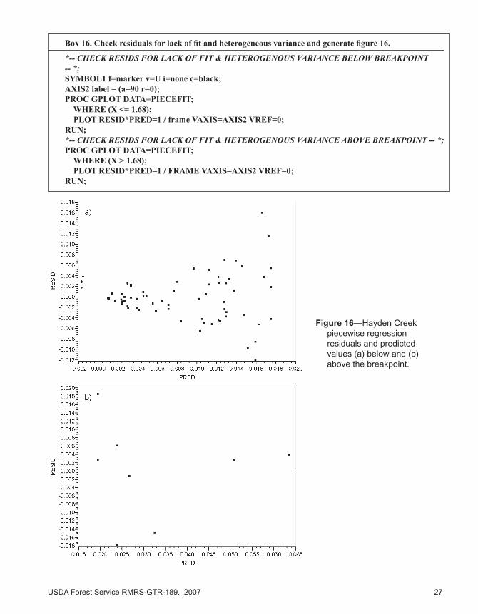
Checking the residuals for homogeneous variance and linearity (box 16), we find that the linearity of the data is not in question because half the data are above and below the line (fig. 16 a, b). However, the variance is not homo-geneous. Since the residuals do not exhibit homogeneous variance, we use bootstrapping methods to obtain appropriate standard errors and confidence intervals for the parameter estimates (a

1, b

1, b

2,c) in the piecewise regression

model (fig. 17, table 6).

Figure 15—QQ-plots for Hayden Creek piecewise regression residuals for curve fits (a) below and (b) above the breakpoint.


Figure 16—Hayden Creek piecewise regression residuals and predicted values (a) below and (b) above the breakpoint.

Box 16. Check residuals for lack of fit and heterogeneous variance and generate figure 16.

*-- CHECK RESIDS FOR LACK OF FIT & HETEROGENOUS VARIANCE BELOW BREAKPOINT -- *;SYMBOL1 f=marker v=U i=none c=black;AXIS2 label = (a=90 r=0);PROC GPLOT DATA=PIECEFIT; WHERE (X <= 1.68); PLOT RESID*PRED=1 / frame VAXIS=AXIS2 VREF=0;RUN;*-- CHECK RESIDS FOR LACK OF FIT & HETEROGENOUS VARIANCE ABOVE BREAKPOINT -- *;PROC GPLOT DATA=PIECEFIT; WHERE (X > 1.68); PLOT RESID*PRED=1 / FRAME VAXIS=AXIS2 VREF=0;RUN;


Potential Outliers

An assessment of potential outliers is important in any analysis. When dealing with measurements of bedload transport, it is common to have outlying data points. However, while a data point should not be removed simply because it is an outlier, it is important to know how these points affect the model fit. Fitting methods such as least absolute deviations (LAD) or iteratively reweighted least squares (IRLS) decrease the affect of outliers on the model fit. For consistency, we use standard least squares to fit the piecewise regression model, but also assess the affect of outliers on the location of the breakpoint. The piecewise model without these extraneous data points is fit and compared against the

Figure 17—Piecewise regression fit between discharge and bedload transport data collected at Hayden Creek with error bars denoting width of 95 percent confidence intervals for the estimated breakpoint.

Table 6—Hayden Creek piecewise regression parameter estimates with corresponding bootstrap estimates of the standard error and 95 percent confidence intervals.

Bootstrap 95% BCa1 Confidence intervals Parameter Estimate standard error (lower, upper)

a1 -0.0077 0.00167 -0.01042 -0.00376

b1 0.0155 0.00211 0.01052 0.01873

b2 0.1067 0.02891 0.02983 0.17383

c 1.6804 0.10540 1.46113 1.80788

1BCa confidence intervals are considered the better bootstrap intervals because they are bettered bias-corrected and accelerated confidence intervals (Efron and Tibshirani 1993).


original fit. When the differences are substantial, the user must determine if the outlying data points should be left in the model or removed for scientific or procedural reasons.

In the Hayden Creek example, two high flow points appear to be very influ-ential observations in fitting the models. If we remove these points and refit the piecewise regression model, the breakpoint moves from 1.68 to 1.0 (fig. 18), providing a very different answer from the original. Additional evidence hints that piecewise model may not be an appropriate model to use in the absence of these data points. For instance, there is only a slight change in slope between the upper and lower modeled segments with the outlying points removed, implying that there may be only one linear segment. Moreover, the calculated MSE for the linear model is not substantially different from the piecewise or power model (table 7), suggesting that a linear fit without these points is as appropriate for these data as the more complex models. Based on this evidence, the range of data in figure 18 likely represents phase I transport and the two outlying data points characterize a limited sampling of phase II transport. More measurements at higher flows would have been beneficial for this data set and demonstrates the importance of obtaining data from a wide range of flows. Furthermore, there is no reason to believe these data points are invalid (in other words there was no instrument or procedural failure) and therefore, we conclude that the original model with all of the data included is the better model for Hayden Creek.

Figure 18—Piecewise regression fit between discharge versus bedload transport data collected at Hayden Creek, with the removal of two high flow observations.


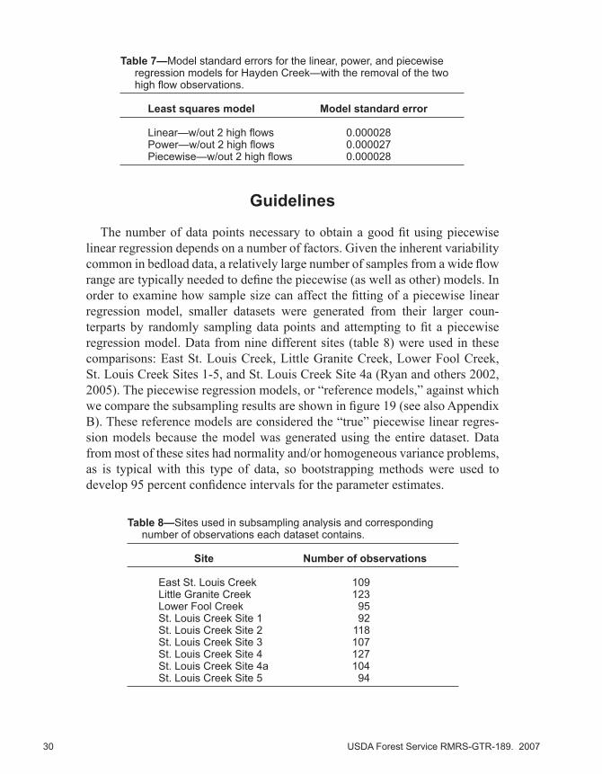
Table 7—Model standard errors for the linear, power, and piecewise regression models for Hayden Creek—with the removal of the two high flow observations.


Linear—w/out 2 high flows 0.000028 Power—w/out 2 high flows 0.000027 Piecewise—w/out 2 high flows 0.000028

Table 8—Sites used in subsampling analysis and corresponding number of observations each dataset contains.

Site Number of observations

East St. Louis Creek 109 Little Granite Creek 123 Lower Fool Creek 95 St. Louis Creek Site 1 92 St. Louis Creek Site 2 118 St. Louis Creek Site 3 107 St. Louis Creek Site 4 127 St. Louis Creek Site 4a 104 St. Louis Creek Site 5 94

Guidelines

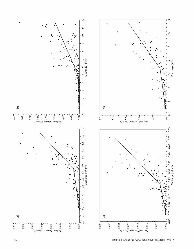
The number of data points necessary to obtain a good fit using piecewise linear regression depends on a number of factors. Given the inherent variability common in bedload data, a relatively large number of samples from a wide flow range are typically needed to define the piecewise (as well as other) models. In order to examine how sample size can affect the fitting of a piecewise linear regression model, smaller datasets were generated from their larger coun-terparts by randomly sampling data points and attempting to fit a piecewise regression model. Data from nine different sites (table 8) were used in these comparisons: East St. Louis Creek, Little Granite Creek, Lower Fool Creek, St. Louis Creek Sites 1-5, and St. Louis Creek Site 4a (Ryan and others 2002, 2005). The piecewise regression models, or “reference models,” against which we compare the subsampling results are shown in figure 19 (see also Appendix B). These reference models are considered the “true” piecewise linear regres-sion models because the model was generated using the entire dataset. Data from most of these sites had normality and/or homogeneous variance problems, as is typical with this type of data, so bootstrapping methods were used to develop 95 percent confidence intervals for the parameter estimates.


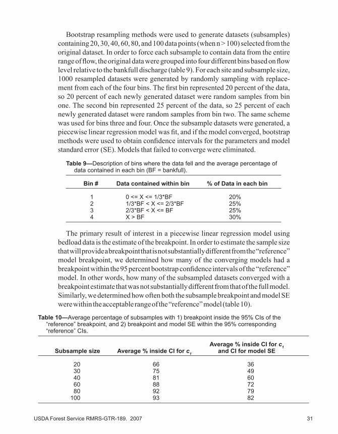
Table 9—Description of bins where the data fell and the average percentage of data contained in each bin (BF = bankfull).

Bin # Data contained within bin % of Data in each bin

1 0 <= X <= 1/3*BF 20% 2 1/3*BF < X <= 2/3*BF 25% 3 2/3*BF < X <= BF 25% 4 X > BF 30%

Table 10—Average percentage of subsamples with 1) breakpoint inside the 95% CIs of the “reference” breakpoint, and 2) breakpoint and model SE within the 95% corresponding “reference” CIs.

Average % inside CI for c1

Subsample size Average % inside CI for c1 and CI for model SE

20 66 36 30 75 49 40 81 60 60 88 72 80 92 79 100 93 82

Bootstrap resampling methods were used to generate datasets (subsamples) containing 20, 30, 40, 60, 80, and 100 data points (when n > 100) selected from the original dataset. In order to force each subsample to contain data from the entire range of flow, the original data were grouped into four different bins based on flow level relative to the bankfull discharge (table 9). For each site and subsample size, 1000 resampled datasets were generated by randomly sampling with replace-ment from each of the four bins. The first bin represented 20 percent of the data, so 20 percent of each newly generated dataset were random samples from bin one. The second bin represented 25 percent of the data, so 25 percent of each newly generated dataset were random samples from bin two. The same scheme was used for bins three and four. Once the subsample datasets were generated, a piecewise linear regression model was fit, and if the model converged, bootstrap methods were used to obtain confidence intervals for the parameters and model standard error (SE). Models that failed to converge were eliminated.

The primary result of interest in a piecewise linear regression model using bedload data is the estimate of the breakpoint. In order to estimate the sample size that will provide a breakpoint that is not substantially different from the “reference” model breakpoint, we determined how many of the converging models had a breakpoint within the 95 percent bootstrap confidence intervals of the “reference” model. In other words, how many of the subsampled datasets converged with a breakpoint estimate that was not substantially different from that of the full model. Similarly, we determined how often both the subsample breakpoint and model SE were within the acceptable range of the “reference” model (table 10).



Fig

ure

19—

Pie

cew

ise

regr

essi

on fi

t for

dis

char

ge v

s. b

edlo

ad tr

ansp

ort a

t (a)

Eas

t St.

Loui

s C

reek

, (b)

Litt

le G

rani

te C

reek

, (c)

Foo

l C

reek

, (d)

St.

Loui

s C

reek

Site

1, (

e) S

t. Lo

uis

Cre

ek S

ite 2

, (f)

St.

Loui

s C

reek

Site

3; (

g) S

t. Lo

uis

Cre

ek S

ite 4

, (h)

St.

Loui

s C

reek

S

ite 4

a, a

nd (

i) S

t. Lo

uis

Cre

ek S

ite 5

.


Figure 19i—continued.


Models developed from subsamples of size 20 had breakpoints within the confidence intervals 66 percent of the time. Requiring the subsamples to have both a breakpoint and model SE within the 95 percent confidence intervals of the “reference” model dropped the percentage to 36 percent (table 10). Notably, there is marked improvement in the percentages of subsamples with a break-point and model SE within the acceptable range at sample size 40. In practice, we observed that datasets containing fewer than 40 data points often have convergence problems, primarily because it is difficult to adequately define transport rates over sub-ranges of flows using fewer measurements. Our results here concur with those observations pertaining to minimum sample size needed to adequately define a breakpoint for bedload data. The benefits of increasing the sample size are not as substantial when the subsample size increases from 60 to 80 data points. Samples of size 60 and 80, when obtained by sampling across the entire range of data, resulted in models with a breakpoint within the 95 percent confidence interval of the “true” breakpoint 88 to 92 percent of the time. Subsamples with both a breakpoint and model SE within the acceptable range of the reference model occurred 72 to 79 percent of the time with samples of size 60 and 80. These results indicate that collecting more than 80 bedload samples does not greatly improve the estimate of the “true” breakpoint. Hence, the cost of obtaining samples where n>80, may not outweigh the benefits in terms of model explanation, as long as the entire flow regime is sampled.

Summary

In this tutorial, we demonstrated the application of piecewise linear regres-sion to bedload data for defining a breakpoint, presumed to represent a shift in phase of transport, so that the reader may perform similar analyses. General statistical theory behind piecewise regression and its procedural approaches were presented, including two examples applied to bedload data from sites in Wyoming and Colorado. The results from a number of additional bedload datasets from St. Louis Creek watershed near Fraser, Colorado were provided to show the range of estimated values and confidence limits on the breakpoint that the analysis provides. Given the inherent variability common in bedload data, a relatively large number of samples from a wide range of flows is needed to define the piecewise regression model. We concluded from a subsampling exercise that a minimum of 40 samples of total bedload transport be obtained for performing the piecewise regression analysis. However, using more than 80 bedload samples did not greatly improve the model’s ability to estimate the “actual” breakpoint. Identification and resolution of common problems encoun-tered in bedload datasets, such as the influence of outliers and other statistical


issues, were also addressed. Data points should not be removed simply because they lie outside of the range of other data, but it is important to know how these points affect the model fit and then judge whether they should be retained. Finally, the code for generating the analysis in SAS provided in bold text in the document has been made available online at the following URL: http://stream.fs.fed.us/publications/software.html.

References

Andrews, E.D. 1984. Bed-material entrainment and hydraulic geometry of gravel-bed rivers in Colorado. Geological Society of America Bulletin. 95: 371-378.

Andrews, E.D.; Nankervis, J.M. 1995. Effective discharge and the design of channel maintenance flows for gravel-bed rivers. In: Costa, J.E.; Miller, A.J.; Potter, K.W.; Wilcock, P.R. eds Natural and Anthropogenic Influences in Fluvial Geomorphology: The Wolman Volume; Geophysical Monograph 89. Washington, DC: American Geophysical Union: 151-164.

Bates, D. M.; Watts, D.G. 1988. Nonlinear Regression Analysis and Its Applications (section 3.10). New York: Wiley. 365 p.

Bunte, K.; Abt, S.R.; Potyondy, J.P.; Ryan, S.E. 2004. Measurement of coarse gravel and cobble transport using a portable bedload trap. Journal of Hydraulic Engineering. 130(9): 879-893.

Efron, B.; Tibshirani, R.J. 1993. An Introduction to the Bootstrap. New York: Chapman and Hill. 436 p.

Emmett, W.W. 1976. Bedload transport in two large, gravel-bed rivers, Idaho and Washington. In: Third Federal Inter-agency Sedimentation Conference: Proceedings; 1976 March 22-25; Denver, CO. 4: 101-114.

Gomez, B.; Naff, R.L.; Hubbell, D.W. 1989. Temporal variations in bedload transport rates associated with the migration of bedforms. Earth Surface Processes and Landforms. 14: 135-156.

Gomez, B.; Hubbell, D.W.; Stevens, H.H. 1990. At-a-point bedload sampling in the presence of dunes. Water Resources Research. 26: 2717-2931.

Jackson, W.L.; Beschta, R.L. 1982. A model of two-phase bedload transport in an Oregon Coast Range stream. Earth Surface Processes and Landforms. 7: 517-527.

Lisle, T.E. 1995. Particle size variations between bed load and bed material in natural gravel bed channels. Water Resources Research. 31(4): 1107-1118.

Neter, J.; Wasserman, W.; Kutner, M.H. 1990. Applied Linear Statistical Models, 3Applied Linear Statistical Models, 3nd ed. Burr Ridge, IL: Irwin. 1181 p.

Paola, C.; Seal, R. 1995. Grain size patchiness as a cause of selective deposition and downstream fining. Water Resources Research. 31(5): 1395-1407.

Parker, G. 1979. Hydraulic geometry of active gravel rivers. Journal of the Hydraulics Division, American Society of Civil Engineers. 105(HY9): 1185-1201.

Parker, G.; Klingeman, P.C. 1982. On why gravel bed streams are paved. WaterOn why gravel bed streams are paved. Water Resources Research. 18: 1409-1423.

Reid, I.; Frostick, L.E. 1986. Dynamics of bedload transport in Turkey Brook, a coarse grained alluvial channel. Earth Surface Processes and Landforms. 11: 143-155.


Ryan, S.E.; Emmett, W.W. 2002. The nature of flow and sediment movement at Little Granite Creek near Bondurant, Wyoming. Gen. Tech. Rep. RMRS-GTR-90. Ogden, UT: U.S. Department of Agriculture, Forest Service, Rocky Mountain Research Station. 48 p.

Ryan, S.E.; Porth, L.S.; Troendle, C.A. 2002. Defining phases of bedload transport using piecewise regression. Earth Surface Processes and Landforms. 27: 971-990.

Ryan, S.E.; Porth, L.S.; Troendle, C.A. 2005. Coarse sediment transport in mountain streams in Colorado and Wyoming, USA. Earth Surface Processes and Landforms. 30: 269-288.

SAS Institute Inc. 2004. SAS/STAT 9.1 User’s Guide. Cary, NC: SAS Institute Inc.Schmidt, L.J.; Potyondy, J.P. 2004. Quantifying channel maintenance instream flows:

an approach for gravel-bed streams in the Western United States. Gen. Tech. Rep. RMRS-GTR-128. Fort Collins, CO: U.S. Department of Agriculture, Forest Service, Rocky Mountain Research Station. 33 p.

Whiting, P.J.; Dietrich, W.E.; Leopold, L.B.; Drake, T.G.; Shreve, R.L. 1988. Bedload sheets in heterogeneous sediment. Geology. 16: 105-108.

Whiting, P.J.; Stamm, J.F.; Moog, D.B.; Orndorff, R.L. 1999. Sediment-transporting flows in headwater streams. Geological Society of America Bulletin. 111(3): 450-466.


Ap

pen

dix

A—

Lit

tle

Gra

nit

e C

reek

exa

mp

le d

atas

et (

x=D

isch

arg

e in

m3

s-1, a

nd

y=

Bed

load

Tra

nsp

ort

in k

g s

-1).

Dat

e x

y

Dat

e x

yD

ate

x y

05/0

8/19

853.

936

0.04

9805

/10/

1990

1.95

40.

0054

05/2

8/19

936.

117

0.07

79

05/1

5/19

852.

945

0.00

9305

/18/

1990

1.55

80.

0006

05/2

8/19

936.

740

0.03

65

05/2

5/19

853.

653

0.01

6505

/25/

1990

2.03

90.

0024

06/0

6/19

934.

390

0.00

18

05/3

0/19

852.

832

0.01

3105

/31/

1990

2.26

60.

0056

06/0

7/19

934.

333

0.01

29

06/0

5/19

851.

926

0.00

3606

/05/

1990

2.03

90.

0062

06/0

8/19

933.

880

0.00

12

06/1

3/19

851.

586

0.00

9706

/14/

1990

1.78

40.

0025

06/0

8/19

933.

795

0.00

11

06/1

9/19

851.

246

0.00

1006

/20/

1990

1.72

80.

0034

06/0

9/19

933.

767

0.00

08

06/2

7/19

850.

821

0.00

0106

/28/

1990

1.47

30.

0035

06/0

9/19

933.

540

0.00

08

07/0

2/19

850.

708

0.00

0207

/05/

1990

0.96

30.

0009

05/2

0/19

977.

878

0.72

26

07/1

1/19

850.

680

0.00

4205

/21/

1991

2.66

20.

0005

05/2

1/19

978.

174

0.26

58

05/1

4/19

862.

011

0.00

6605

/21/

1991

2.66

20.

0013

05/2

1/19

979.

799

0.65

20

05/2

8/19

868.

439

0.34

0205

/29/

1991

2.83

20.

0006

05/2

2/19

978.

546

0.49

45

06/0

3/19

8611

.413

0.29

9206

/01/

1991

2.43

60.

0008

05/2

2/19

979.

232

0.36

54

06/1

2/19

867.

080

0.01

1006

/01/

1991

2.43

60.

0007

05/2

8/19

976.

186

0.07

79

06/1

8/19

865.

098

0.00

6006

/01/

1991

2.37

90.

0018

05/2

9/19

976.

868

0.43

79

06/2

6/19

862.

945

0.00

4706

/03/

1991

3.14

30.

0066

05/2

9/19

977.

078

0.45

82

07/0

2/19

862.

351

0.00

7706

/03/

1991

4.22

00.

0065

05/3

0/19

977.

494

0.05

52

07/1

0/19

861.

614

0.00

0806

/03/

1991

3.96

50.

0121

05/3

0/19

977.

447

0.08

53

07/1

6/19

861.

303

0.00

1106

/04/

1991

5.18

30.

0265

05/3

0/19

978.

864

0.24

32

05/1

3/19

871.

756

0.00

7406

/04/

1991

5.38

10.

0212

05/3

1/19

977.

780

0.08

80

05/2

2/19

871.

869

0.01

0906

/11/

1991

4.05

00.

0043

05/3

1/19

978.

125

0.14

12

05/2

8/19

873.

002

0.05

1506

/11/

1991

4.05

00.

0059

05/3

1/19

979.

421

0.24

98

06/0

3/19

872.

096

0.00

9106

/11/

1991

4.07

80.

0051

06/0

1/19

9710

.302

0.20

01

05/1

2/19

881.

926

0.00

5706

/11/

1991

4.47

50.

0046

06/0

1/19

9710

.050

0.18

31

05/1

8/19

884.

418

0.01

6206

/12/

1991

4.24

80.

0095

06/0

1/19

979.

862

0.13

97

05/2

7/19

884.

220

0.01

0806

/12/

1991

3.93

60.

0086

06/0

4/19

9711

.243

0.91

44

06/0

3/19

882.

124

0.01

1206

/12/

1991

4.19

10.

0050

06/0

5/19

979.

950

0.83

52

06/1

0/19

881.

671

0.00

1006

/12/

1991

4.36

10.

0072

06/0

5/19

9710

.025

1.00

60

06/1

5/19

881.

359

0.00

1106

/12/

1991

4.50

30.

0063

06/0

5/19

9711

.158

1.07

82

06/2

2/19

881.

161

0.00

0506

/12/

1991

4.70

10.

0075

06/0

5/19

9711

.561

1.42

96

05/0

5/19

892.

379

0.00

9806

/13/

1991

4.41

80.

0049

06/0

6/19

979.

723

0.56

08

05/0

9/19

894.

899

0.06

0306

/13/

1991

4.30

50.

0032

06/0

6/19

979.

295

0.63

10

05/1

8/19

894.

361

0.06

2306

/13/

1991

4.13

50.

0093

06/1

0/19

977.

233

0.43

04

05/2

5/19

893.

880

0.04

0906

/05/

1992

0.73

60.

0000

06/1

1/19

976.

137

0.49

02

06/0

2/19

893.

370

0.00

4306

/06/

1992

0.73

60.

0001

06/1

1/19

976.

137

0.56

76

06/0

7/19

894.

701

0.03

0606

/07/

1992

0.70

80.

0002

06/1

1/19

976.

039

0.58

71

06/1

5/19

893.

455

0.00

3906

/08/

1992

0.70

80.

0001

06/1

2/19

975.

642

0.10

95

06/2

1/19

892.

209

0.00

1505

/26/

1993

5.55

10.

0428

06/1

2/19

975.

504

0.08

86

06/2

9/19

891.

473

0.00

0105

/26/

1993

5.15

40.

0774

06/1

2/19

975.

689

0.11

12

07/0

5/19

891.

274

0.00

0105

/27/

1993

6.14

50.

0217

06/1

3/19

975.

089

0.05

81

04/2

7/19

901.

529

0.00

2705

/27/

1993

6.25

90.

0248

06/1

3/19

974.

918

0.04

99


Dat

e x

y

Dat

e x

yD

ate

x y

05/0

8/19

853.

936

0.04

9805

/10/

1990

1.95

40.

0054

05/2

8/19

936.

117

0.07

79

05/1

5/19

852.

945

0.00

9305

/18/

1990

1.55

80.

0006

05/2

8/19

936.

740

0.03

65

05/2

5/19

853.

653

0.01

6505

/25/

1990

2.03

90.

0024

06/0

6/19

934.

390

0.00

18

05/3

0/19

852.

832

0.01

3105

/31/

1990

2.26

60.

0056

06/0

7/19

934.

333

0.01

29

06/0

5/19

851.

926

0.00

3606

/05/

1990

2.03

90.

0062

06/0

8/19

933.

880

0.00

12

06/1

3/19

851.

586

0.00

9706

/14/

1990

1.78

40.

0025

06/0

8/19

933.

795

0.00

11

06/1

9/19

851.

246

0.00

1006

/20/

1990

1.72

80.

0034

06/0

9/19

933.

767

0.00

08

06/2

7/19

850.

821

0.00

0106

/28/

1990

1.47

30.

0035

06/0

9/19

933.

540

0.00

08

07/0

2/19

850.

708

0.00

0207

/05/

1990

0.96

30.

0009

05/2

0/19

977.

878

0.72

26

07/1

1/19

850.

680

0.00

4205

/21/

1991

2.66

20.

0005

05/2

1/19

978.

174

0.26

58

05/1

4/19

862.

011

0.00

6605

/21/

1991

2.66

20.

0013

05/2

1/19

979.

799

0.65

20

05/2

8/19

868.

439

0.34

0205

/29/

1991

2.83

20.

0006

05/2

2/19

978.

546

0.49

45

06/0

3/19

8611

.413

0.29

9206

/01/

1991

2.43

60.

0008

05/2

2/19

979.

232

0.36

54

06/1

2/19

867.

080

0.01

1006

/01/

1991

2.43

60.

0007

05/2

8/19

976.

186

0.07

79

06/1

8/19

865.

098

0.00

6006

/01/

1991

2.37

90.

0018

05/2

9/19

976.

868

0.43

79

06/2

6/19

862.

945

0.00

4706

/03/

1991

3.14

30.

0066

05/2

9/19

977.

078

0.45

82

07/0

2/19

862.

351

0.00

7706

/03/

1991

4.22

00.

0065

05/3

0/19

977.

494

0.05

52

07/1

0/19

861.

614

0.00

0806

/03/

1991

3.96

50.

0121

05/3

0/19

977.

447

0.08

53

07/1

6/19

861.

303

0.00

1106

/04/

1991

5.18

30.

0265

05/3

0/19

978.

864

0.24

32

05/1

3/19

871.

756

0.00

7406

/04/

1991

5.38

10.

0212

05/3

1/19

977.

780

0.08

80

05/2

2/19

871.

869

0.01

0906

/11/

1991

4.05

00.

0043

05/3

1/19

978.

125

0.14

12

05/2

8/19

873.

002

0.05

1506

/11/

1991

4.05

00.

0059

05/3

1/19

979.

421

0.24

98

06/0

3/19

872.

096

0.00

9106

/11/

1991

4.07

80.

0051

06/0

1/19

9710

.302

0.20

01

05/1

2/19

881.

926

0.00

5706

/11/

1991

4.47

50.

0046

06/0

1/19

9710

.050

0.18

31

05/1

8/19

884.

418

0.01

6206

/12/

1991

4.24

80.

0095

06/0

1/19

979.

862

0.13

97

05/2

7/19

884.

220

0.01

0806

/12/

1991

3.93

60.

0086

06/0

4/19

9711

.243

0.91

44

06/0

3/19

882.

124

0.01

1206

/12/

1991

4.19

10.

0050

06/0

5/19

979.

950

0.83

52

06/1

0/19

881.

671

0.00

1006

/12/

1991

4.36

10.

0072

06/0

5/19

9710

.025

1.00

60

06/1

5/19

881.

359

0.00

1106

/12/

1991

4.50

30.

0063

06/0

5/19

9711

.158

1.07

82

06/2

2/19

881.

161

0.00

0506

/12/

1991

4.70

10.

0075

06/0

5/19

9711

.561

1.42

96

05/0

5/19

892.

379

0.00

9806

/13/

1991

4.41

80.

0049

06/0

6/19

979.

723

0.56

08

05/0

9/19

894.

899

0.06

0306

/13/

1991

4.30

50.

0032

06/0

6/19

979.

295

0.63

10

05/1

8/19

894.

361

0.06

2306

/13/

1991

4.13

50.

0093

06/1

0/19

977.

233

0.43

04

05/2

5/19

893.

880

0.04

0906

/05/

1992

0.73

60.

0000

06/1

1/19

976.

137

0.49

02

06/0

2/19

893.

370

0.00

4306

/06/

1992

0.73

60.

0001

06/1

1/19

976.

137

0.56

76

06/0

7/19

894.

701

0.03

0606

/07/

1992

0.70

80.

0002

06/1

1/19

976.

039

0.58

71

06/1

5/19

893.

455

0.00

3906

/08/

1992

0.70

80.

0001

06/1

2/19

975.

642

0.10

95

06/2

1/19

892.

209

0.00

1505

/26/

1993

5.55

10.

0428

06/1

2/19

975.

504

0.08

86

06/2

9/19

891.

473

0.00

0105

/26/

1993

5.15

40.

0774

06/1

2/19

975.

689

0.11

12

07/0

5/19

891.

274

0.00

0105

/27/

1993

6.14

50.

0217

06/1

3/19

975.

089

0.05

81

04/2

7/19

901.

529

0.00

2705

/27/

1993

6.25

90.

0248

06/1

3/19

974.

918

0.04

99


Appendix B—Piecewise regression results with bootstrap confidence intervals.

Watershed Parameter Estimate Lower 95% CI Upper 95% CI

East St. Louis Ck SE 0.0098 0.0074 0.0115 a

1 -0.0023 -0.0047 -0.0010

b1 0.0109 0.0072 0.0174

b2 0.0735 0.0442 0.1367

c1 0.7572 0.6733 0.8933

Fool Creek SE 0.0050 0.0037 0.0061 a

1 -0.0009 -0.0014 0.0002

b1 0.0172 0.0044 0.0227

b2 0.0856 0.0653 0.1061

c1 0.2211 0.1696 0.2580

Little Granite Ck SE 0.1609 0.1253 0.1912 a

1 -0.0037 -0.0330 -0.0003

b1 0.0043 0.0024 0.0173

b2 0.1046 0.0753 0.1851

c1 4.8446 4.1345 6.9900

Site 1 SE 0.0539 0.0383 0.0646 a

1 -0.0055 -0.0157 0.0013

b1 0.0139 0.0074 0.0223

b2 0.0730 0.0454 0.1472

c1 3.4118 2.4869 4.6944

Site 2 SE 0.0549 0.0382 0.0686 a

1 -0.0069 -0.0180 -0.0026

b1 0.0118 0.0086 0.0192

b2 0.1222 0.0941 0.2159

c1 4.4992 4.3024 5.4983

Site 3 SE 0.0702 0.0398 0.0940 a

1 -0.0187 -0.0283 -0.0046

b1 0.0198 0.0080 0.0265

b2 0.0775 0.0432 0.1565

c1 4.0421 2.5055 4.9058


Site 4 SE 0.0222 0.0170 0.0263 a

1 -0.000004 -0.0069 0.0098

b1 0.0037 -0.0037 0.0092

b2 0.0228 0.0185 0.0318

c1 1.8972 1.6442 2.5725

Site 4a SE 0.0299 0.0230 0.0353 a

1 -0.0101 -0.0182 0.0085

b1 0.0124 -0.0001 0.0173

b2 0.0515 0.0368 0.0679

c1 2.8074 2.1699 3.1024

Site 5 SE 0.0142 0.0090 0.0179 a

1 -0.00001 -0.0027 0.0031

b1 0.0036 0.0014 0.0057

b2 0.0437 0.0301 0.0811

c1 2.3545 2.1424 2.6587

(numbers highlighted are those where the intercept is not significantly different from zero and

could be removed from model).

Watershed Parameter Estimate Lower 95% CI Upper 95% CI

The Rocky Mountain Research Station develops scientific information and technology to improve management, protection, and use of the forests and rangelands. Research is designed to meet the needs of the National Forest managers, Federal and State agencies, public and private organizations, academic institutions, industry, and individuals.

Studies accelerate solutions to problems involving ecosystems, range, forests, water, recreation, fire, resource inventory, land reclamation, community sustainability, forest engineering technology, multiple use economics, wildlife and fish habitat, and forest insects and diseases. Studies are conducted cooperatively, and applications may be found worldwide.

Research Locations

Flagstaff, Arizona Reno, NevadaFort Collins, Colorado* Albuquerque, New MexicoBoise, Idaho Rapid City, South DakotaMoscow, Idaho Logan, UtahBozeman, Montana Ogden, UtahMissoula, Montana Provo, Utah

*Station Headquarters, Natural Resources Research Center, 2150 Centre Avenue, Building A, Fort Collins, CO 80526.

The U.S. Department of Agriculture (USDA) prohibits discrimination in all its pro-grams and activities on the basis of race, color, national origin, age, disability, and where applicable, sex, marital status, familial status, parental status, religion, sexual orientation, genetic information, political beliefs, reprisal, or because all or part of an individual’s income is derived from any public assistance program. (Not all prohibited bases apply to all programs.) Persons with disabilities who require alternative means for communication of program information (Braille, large print, audiotape, etc.) should contact USDA’s TARGET Center at (202) 720-2600 (voice and TDD). To file a complaint of discrimination, write to USDA, Director, Office of Civil Rights, 1400 Independence Avenue, S.W., Washington, DC 20250-9410, or call (800) 795-3272 (voice) or (202) 720-6382 (TDD). USDA is an equal opportu-nity provider and employer.

Federal Recycling Program Printed on Recycled Paper

RMRSROCKY MOUNTAIN RESEARCH STATION

Date post:	03-Feb-2022
Category:	Documents
Upload:	others
View:	2 times
Download:	0 times

A tutorial on the piecewise regression approach applied to bedload

Documents