Qiyuan Tian and Haomiao Jiang Department of Electrical Engineering Stanford University GPU Technology Conference, San Jose March 17, 2015 Accelerating a learning–based image processing pipeline for digital cameras Local, Linear and Learned (L 3 ) pipeline
Transcript
Qiyuan Tian and Haomiao Jiang
Department of Electrical Engineering
Stanford University
GPU Technology Conference, San Jose
March 17, 2015
Accelerating a learning–based image processing pipeline for digital cameras Local, Linear and Learned (L3) pipeline
Digital camera sub-systems
Focus
control
Exposure
control
Lens, aperture and
sensor
Pre-processing • dead pixel removal
• dark floor subtraction
• structured noise reduction
• quantization
• etc.
RAW image Display image
Image
processing
pipeline
Transform the
sensor data
into a display image
CFA
Standard image processing pipeline
RAW image Display image
CFA
interpolation
Sensor
conversion
Illuminant
correction
Tone
scale
Noise
reduction
− Requires multiple algorithms
− Each algorithm requires optimization
− Optimized only for Bayer (RGB) color filter array (CFA)
Opportunity
Extra sensor pixels enable new CFAs that improve sensor functionality and open new applications
Challenge − Customized image processing pipeline
− Speed and low power
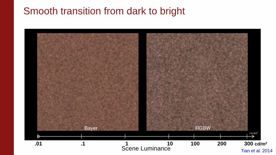
Bayer
RGBX
infrared
light field
RGBW
low-light sensitivity
dynamic range
Medical
specialized
application
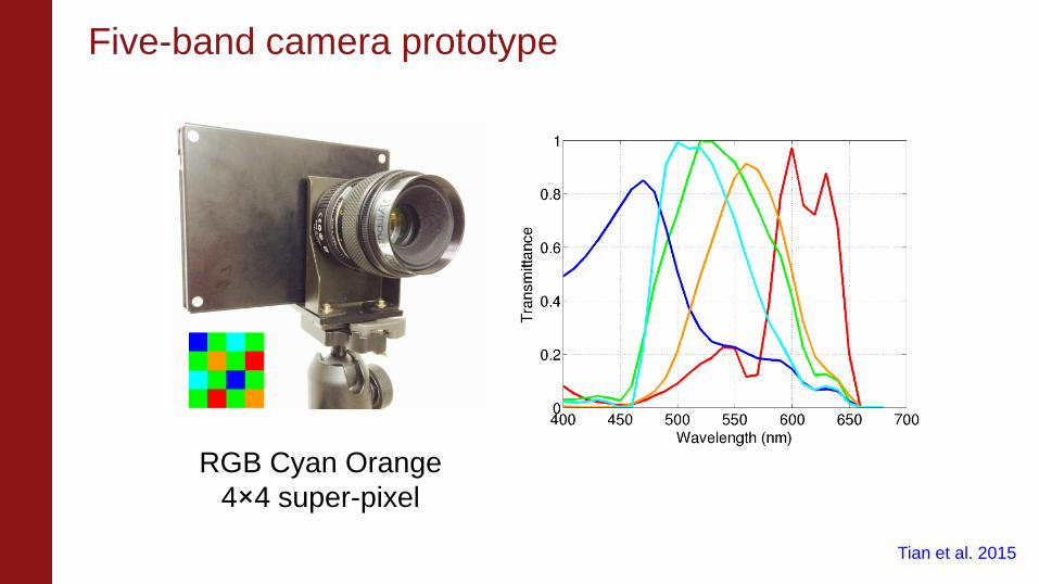
RGBCMY
multispectral
Sensor
conversion
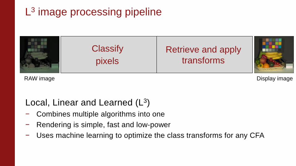
L3 image processing pipeline
Local, Linear and Learned (L3)
− Combines multiple algorithms into one
− Rendering is simple, fast and low-power
− Uses machine learning to optimize the class transforms for any CFA
RAW image Display image
CFA
interpolation
Illuminant
correction
Tone
scale
Noise
reduction
Classify
pixels Retrieve and apply
transforms
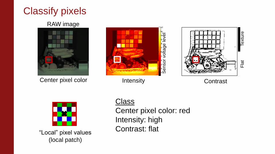
Classify pixels
Se
nso
r vo
lta
ge
leve
l
Intensity
Fla
t
Te
xtu
re
Contrast
Class
Center pixel color: red
Intensity: high
Contrast: flat
Center pixel color
RAW image
“Local” pixel values
(local patch)
Retrieve and apply transforms
Class
Center pixel color: red
Intensity: high
Contrast: flat
Contrast
Inte
nsity Learned
table of
linear
transforms
Weighted summation
Rendered
R, G, B values
RAW image R G B “Linear” transforms
Table-based architecture suits GPU
Weighted summation Weighted summation
− Independent calculation for each pixel
− Simple weighted summation
Thus well-suited for parallel rendering using GPU
GPU
GPU implementations
Table of transforms
Render one pixel (i, j)
• Calculate class index
• Retrieve transforms
• Weight sum
Constants, e.g. CFA pattern
GPU acceleration results
− GPU: NVidia GTX 770 (1536 kernels, 1.085 GHz)
− CPU: Intel Core i7-4770K (3.5 GHz)
− CUDA/C programming
Results CPU GPU
Image
(1280×720) 12.4s
0.062s
(16 fps)
Video
(1280×720×1800)
163.2s
(11 fps)
Tian et al. 2015
Potential speed improvement
Use shared memory and registers
Specialized image signal processor (ISP)
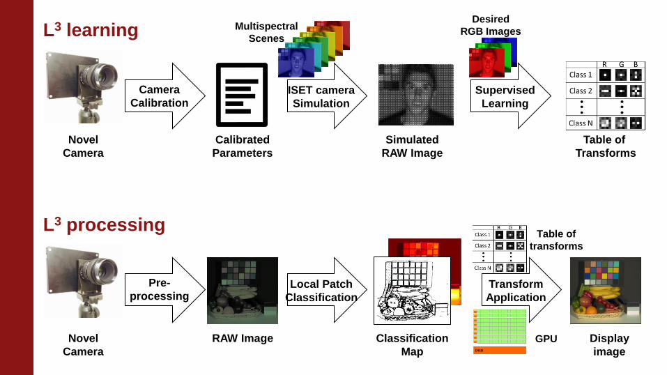
L3 ISP
Novel
Camera
Pre-
processing Local Patch
Classification
Transform
Application
RAW Image Classification
Map
Display
image
Table of
Transforms
GPU
“Learn” the transforms L3 processing
Locally linear transform
Contrast Center color Intensity
Local
patches
red
white
green
blue
flat
texture
0 V
1 V
20 levels
− Globally nonlinear for an entire image
− 480 linear transforms in total
Learn the locally linear transform for each class
R G B
Linear
transform Local RAW
values
Desired RGB
values
A 𝐱 = 𝐛
?
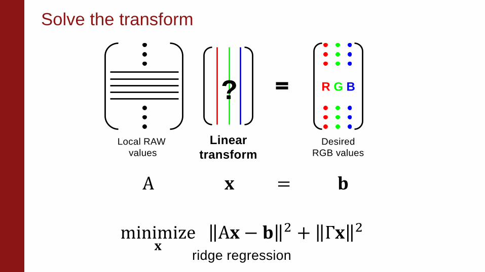
Solve the transform
R G B
Local RAW
values
Desired
RGB values
minimize𝐱
A𝐱 − 𝐛 2 + Γ𝐱 2
Linear
transform
?
ridge regression
A 𝐱 = 𝐛
?
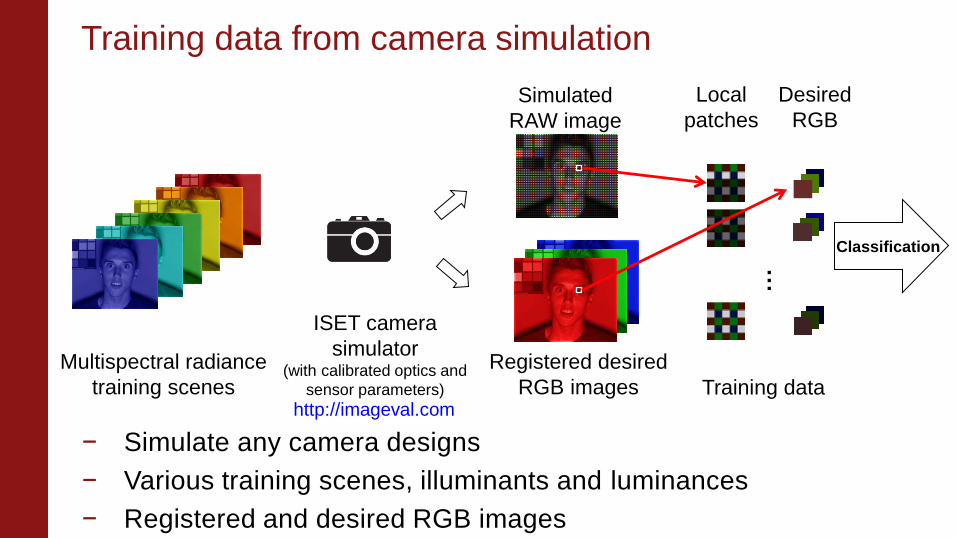
Training data from camera simulation
Multispectral radiance
training scenes
ISET camera
simulator (with calibrated optics and
sensor parameters)
Simulated
RAW image
Registered desired
RGB images
…
Training data
Classification
Local
patches
Desired
RGB
− Simulate any camera designs
− Various training scenes, illuminants and luminances