The inverse scattering series (ISS) is a direct inversion method for a multidimensional acoustic,elastic and anelastic earth. It communicates that all inversion processing goals can beachieved directly and without any subsurface information. This task is reached through a task specificsubseries of the ISS. Using primaries in the data as sub events of the first-order internalmultiples, the leading-order attenuator can predict the time of all the first-order internal multiplesand is able to attenuate them.
14
Accuracy of the internal multiple prediction when a time-saving method based on two angular quantities (angle constraints) is applied to the ISS internal multiple attenuation algorithm Hichem Ayadi and Arthur B. Weglein April 29, 2013 Abstract The inverse scattering series (ISS) is a direct inversion method for a multidimensional acous- tic, elastic and anelastic earth. It communicates that all inversion processing goals can be achieved directly and without any subsurface information. This task is reached through a task- specific subseries of the ISS. Using primaries in the data as subevents of the first-order internal multiples, the leading-order attenuator can predict the time of all the first-order internal multi- ples and is able to attenuate them. However, the ISS internal multiple attenuation algorithm can be a computationally demanding method, especially in a complex earth. By using an approach that is based on two angular quantities and that was proposed in Terenghi et al. (2012), the cost of the algorithm can be controlled. The idea is to use the two angles as key-control parameters, by limiting their varia- tion, to disregard some calculated contributions of the algorithm that are negligible. Moreover, the range of integration can be chosen as a compromise of the required degree of accuracy and the computational time saving. This time-saving approach is presented in this report and applied to the ISS internal multiple attenuation algorithm. Through a numerical analysis, the relationship between accuracy and performance is examined and discussed. 1 Introduction In exploration seismology, a source of energy generated on or near the surface of the earth or of water produces waves that propagate into the subsurface. The wave travels through the earth until it hits a rock layer or a material with a different impedance. A part of the energy is reflected back towards the surface and is recorded at the measurement surface by geophones or hydrophones. An arrival of seismic energy is called an event. An event that experiences just one upward reflection is a primary. A ghost is an event that starts its path by propagating up from the source and reflecting down from the free surface (a source ghost), or ends its path by propagating down to the receiver (a receiver ghost). An event that experiences more that one downward reflection is a multiple. We consider two kinds of multiples. A free-surface multiple is a multiple that experiences more than one upward reflection and at least one downward reflection at the air-water or air-land surface. An internal multiple is an event that experiences more than one upward reflection and all downward 120
Transcript
Accuracy of the internal multiple prediction when a time-saving method basedon two angular quantities (angle constraints) is applied to the ISS internal
multiple attenuation algorithm
Hichem Ayadi and Arthur B. Weglein
April 29, 2013
Abstract
The inverse scattering series (ISS) is a direct inversion method for a multidimensional acous-tic, elastic and anelastic earth. It communicates that all inversion processing goals can beachieved directly and without any subsurface information. This task is reached through a task-specific subseries of the ISS. Using primaries in the data as subevents of the first-order internalmultiples, the leading-order attenuator can predict the time of all the first-order internal multi-ples and is able to attenuate them.However, the ISS internal multiple attenuation algorithm can be a computationally demandingmethod, especially in a complex earth. By using an approach that is based on two angularquantities and that was proposed in Terenghi et al. (2012), the cost of the algorithm can becontrolled. The idea is to use the two angles as key-control parameters, by limiting their varia-tion, to disregard some calculated contributions of the algorithm that are negligible. Moreover,the range of integration can be chosen as a compromise of the required degree of accuracy andthe computational time saving.This time-saving approach is presented in this report and applied to the ISS internal multipleattenuation algorithm. Through a numerical analysis, the relationship between accuracy andperformance is examined and discussed.
1 Introduction
In exploration seismology, a source of energy generated on or near the surface of the earth or ofwater produces waves that propagate into the subsurface. The wave travels through the earth untilit hits a rock layer or a material with a different impedance. A part of the energy is reflected backtowards the surface and is recorded at the measurement surface by geophones or hydrophones. Anarrival of seismic energy is called an event. An event that experiences just one upward reflection isa primary. A ghost is an event that starts its path by propagating up from the source and reflectingdown from the free surface (a source ghost), or ends its path by propagating down to the receiver(a receiver ghost). An event that experiences more that one downward reflection is a multiple. Weconsider two kinds of multiples. A free-surface multiple is a multiple that experiences more thanone upward reflection and at least one downward reflection at the air-water or air-land surface. Aninternal multiple is an event that experiences more than one upward reflection and all downward
120
Multiple attenuation part I M-OSRP12
reflections from below the free surface. Ghosts and multiples are considered to be noise. A primaryhas only one upward reflection, which makes it relatively easy to extract information from aboutthe subsurface.In this report we will focus only on the study of primaries and internal multiples.
Araújo et al. (1994) and Weglein et al. (1997) have proposed the ISS internal-multiple-attenuationalgorithm. It is a leading-order contribution towards the elimination of first-order internal multi-ples. The algorithm is based on the construction of an internal-multiple attenuator coming froma subseries of the ISS. It has received positive attention for stand-alone capability for attenuatingfirst-order internal multiples in marine and offshore plays.
Terenghi et al. (2012) introduced two angular quantities that can be used as a key-control parameteron the computational cost of the ISS leading-order internal-multiple-attenuation algorithm. Thetwo angles, α (the dip of the reflection in the subsurface) and γ (the incidence angle between thepropagation vector of a wave and the normal to the reflector), are related to the wavefield variablesin the f-k domain. Therefore, control of this angle can be key to our ability to control the timeloop of the algorithm. That has been discussed by Terenghi et al. (2012). In this report, we willdiscuss how the computational cost can relate to the accuracy of internal-multiple prediction. Inother words, is it possible to reduce the computational time of the ISS internal-multiple attenuationalgorithm without affecting its efficiency?
In the first part of this report, a description of the internal-multiple-attenuation algorithm will beprovided. It discusses how the first-order internal-multiple attenuator can be constructed from asubseries of the ISS. Then, the computational cost savings proposed by Terenghi et al. (2012) willbe developed and applied to the ISS internal-multiple-attenuation algorithm. Finally, a numericalanalysis will be presented, in order to discuss the accuracy and efficiency of the algorithm with thiskey control.
2 The ISS internal multiple attenuation algorithm
In seismic processing, many processing methods make assumptions and require subsurface infor-mation. However, sometimes these assumptions are difficult or impossible to satisfy in a complexworld. Furthermore, when the assumptions are not satisfied, the method is not functional. Theinverse scattering series states that all processing objectives can be achieved directly and withoutany subsurface information.The inverse scattering series is based on scattering theory, which is a form of perturbation analysis.It describes how a scattered wavefield (the difference between the actual wavefield and the referencewavefield) relates to the perturbation (the difference between the actual medium and the referencemedium).
The forward scattering series construction starts with the differential equations governing wavepropagation in the media:
LG = δ(r − rs), (2.1)
L0G0 = δ(r − rs). (2.2)
121
Multiple attenuation part I M-OSRP12
Where L and L0 are the actual and the reference differential operators, respectively, and G and G0
are the actual and reference GreenâĂŹs functions, respectively.
Define the scattered field as ψs = G−G0 and the perturbation as V = L0 − L.The Lippmann-Schwinger equation relates G, G0, and V :
G = G0 +G0V G (2.3)
Substituting iteratively the Lippmann-Schwinger equation into itself gives the forward scatteringseries:
where, (ψn) is the portion of the scattered wavefield that is the nth order in V . The measuredvalues of ψs are the data D.
The perturbation V can also be expanded as a series,
V = V1 + V2 + V3 + ... (2.5)
Substituting V into the forward scattering series and evaluating the scattered field on the measure-ment surface results in the inverse scattering series:
the inverse scattering series internal-multiple-attenuation concept is based on the analogy betweenthe forward series and the inverse series. The forward series could generate primaries and internalmultiples through the action of G0 on the perturbation V , while, the inverse series can achieve afull inversion of V by using G0 and the measured data. The way that G0 acts on the perturbationto construct the internal multiples suggests the way to remove them.In the forward series, the first-order internal multiples have their leading-order contribution fromthe third term: G0V G0V G0V G0. This suggests that the leading-order attenuator of internal mul-tiples can be found in the third term in the inverse series equation (2.8). In Weglein et al. (1997)a subseries that attenuates internal multiples was identified and separated from the entire inversescattering series.
The ISS internal-multiple-attenuation algorithm is a subseries of the inverse scattering series. Thealgorithm begins with the input data D(kg, ks, ω), which are the data in the ω temporal frequencydeghosted and with free-surface multiple removed. Here ks, kg are the source and receiver horizontalwavenumber, respectively. Then, let us define b1(kg, ks, ω) which corresponds to an uncollapsed f-kmigration of effective incident plane-wave data as
b1(kg, ks, ω) = (−2iqs)D(kg, ks, ω) (2.9)
122
Multiple attenuation part I M-OSRP12
where qs = sgn(ω)√
( ωc0 )2 − ks is the sourceâĂŹs vertical wavenumber and c0 the reference velocity.The second term in the algorithm is the leading-order attenuator b3, which attenuates all the first-order internal multiples. The leading-order attenuator for a 2D earth is given by,
b3(ks, kg, ω) =1
(2π)2
∫ +∞
−∞dk1
∫ +∞
−∞dk2e
−iq1(zg−zs)e−iq2(zg−zs)
∫ +∞
−∞dz1b1(kg, k1, z1)ei(qg+q1)z1
∫ z1−ε
−∞dz2b1(k1, k2, z2)e−i(q1+q2)z2
∫ +∞
z2+εdz3b1(k2, ks, z3)ei(q2+qs)z3
(2.10)
where z1, z2, and z3 are the pseudo-depths. ε is a small positive parameter chosen in order to makesure that z1 > z2 and z3 > z2 are satisfied.
Finally, using the input data and the leading-order attenuator of the first-order internal multiples,the data with the first-order internal multiples attenuated is given by
D(kg, ks, ω) +D3(kg, ks, ω) (2.11)
with D3(kg, ks, ω) = (−2iqs)−1b3(kg, ks, ω).
3 Computational cost saving using two angle constraints.
Terenghi et al. (2012) discuss two angular quantities that can be used in order to reduce thecomputational cost of the ISS internal-multiple-attenuator algorithm. The idea is to constructkey-control parameters that allow to disregard some part of the calculus that is insignificant duringthe computation. In other words, use this key-parameters to optimize some intervals of calculus inthe algorithm. The approach used is based on certain angular quantities in order to control the costof the algorithm.
Stolt and Weglein (2012) define the image-function wavenumber as a difference between the receiverand source-side wavenumbers
~km = ~kg − ~ks = ( ~κg − ~κg, qg − qs) (3.1)
Here ~κs and ~κg are the horizontal components of the source and receiver wavenumbers, respectively.
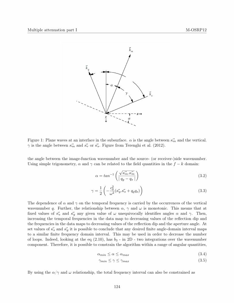
This definitions allows the construction of two angles, α and γ (cf. Figure 1). The dip angle αcorresponds to the angle between the surface and the horizontal component. The incident angle γ is
123
Multiple attenuation part I M-OSRP12
Figure 1: Plane waves at an interface in the subsurface. α is the angle between ~κm and the vertical.γ is the angle between ~κm and ~κr or ~κs. Figure from Terenghi et al. (2012).
the angle between the image-function wavenumber and the source- (or receiver-)side wavenumber.Using simple trigonometry, α and γ can be related to the field quantities in the f − k domain:
α = tan−1
( √~κm. ~κm
| qg − qs |
)(3.2)
γ =1
2
(− c
20
ω2( ~κg. ~κs + qgqs)
)(3.3)
The dependence of α and γ on the temporal frequency is carried by the occurrences of the verticalwavenumber q. Further, the relationship between α, γ and ω is monotonic. This means that atfixed values of ~κs and ~κg any given value of ω unequivocally identifies angles α and γ. Then,increasing the temporal frequencies in the data map to decreasing values of the reflection dip andthe frequencies in the data maps to decreasing values of the reflection dip and the aperture angle. Atset values of ~κs and ~κg it is possible to conclude that any desired finite angle-domain interval mapsto a similar finite frequency domain interval. This may be used in order to decrease the numberof loops. Indeed, looking at the eq (2.10), has b3 - in 2D - two integrations over the wavenumbercomponent. Therefore, it is possible to constrain the algorithm within a range of angular quantities,
αmin ≤ α ≤ αmax (3.4)γmin ≤ γ ≤ γmax (3.5)
By using the α/γ and ω relationship, the total frequency interval can also be constrained as
Then, the reduction of the total frequency interval allows us to reduce the interval of integration ofb3 and which means reducing the number of loops.
Figure 2: Process of the ISS internal multiple attenuation with angle constraints.
The Figure 2 recapitulates in a graph all of the process described previously. In the next section,a numerical analysis continues and illustrates the discussion from sections 2 and 3, in which theefficiency and accuracy of the angle-constraints method are presented.
125
Multiple attenuation part I M-OSRP12
4 Numerical analysis
In this section numerical examples are shown in order to illustrate the concepts previously presented.The model considered in this numerical analysis is a three layer earth at depths : z = 1000m, 1300mand 1700m. The source shot (z = 910 and x = 6086) is recorded by 928 receivers. The maximumoffset is at 2320m. Figure 3 shows the shot gather with the different events: primaries (green array)and internal multiples.
Figure 3: Shot gather recorded. The three primaries resulting from the three layers are shown ingreen.
Figure 4, illustrates the internal-multiple prediction using the ISS internal multiple attenuationalgorithm. All first-order the internal multiple are predicted.
Figure 6 illustrates the internal-multiple prediction following the process uses angle constraints, asshown in the Figure 2. The model is in 1D; consequently, just one angle (the incident angle γ) canbe constraint. The analysis made in 1D for γ can be extended to α by analogy.
A first interpretation would be that we do not need to compute for a full open angle in order tohave an accurate prediction of the internal multiples. Notice that a prediction with a full openangle corresponds to an internal multiple prediction without any angle constraints. Even so, withreduction to a certain angle (γlimite) the prediction of the internal multiples is degraded.
Figure 7 shows the amplitude for different γmax angles at zero offset and comparing with theamplitude for a full open γ-angle. It is clear that the amplitude, at zero offset, is not affected. Thefirst-order internal multiple are predicted at the right time and the right amplitude.
126
Multiple attenuation part I M-OSRP12
Figure 4: Prediction of all the first-order internal multiples.
Figure 8 plots the amplitude for different values of γmax at offset 1405m and comparing with theamplitude for a full open γ-angle. In Figure 6, the prediction of the internal multiples for γmax = 20◦
seems to be the same as that for γmax = 25◦ and Figure 4. If we look more precisely at the amplitude,we can see that it has been affected. The amplitude for γmax = 20◦ does not correspond exactly tothe amplitude for γmax = 90, for the same trace number. However, for γmax = 25◦, the amplitudeis exactly the same as that for the full open Îş angle. Notice that even if the amplitude is affected,the internal multiple are still predicted at the right time.
If we look at the shape (cf. Figure 9), the same interpretation can be made. For γmax = 25◦ theshape matches with an usual internal multiple prediction (full open γ-angle). Bellow this incidentangle, the shape do not match which means that the prediction can not be considered accurate.
127
Multiple attenuation part I M-OSRP12
Figure 5: Computational time in function of the incident angle chosen.
128
Multiple attenuation part I M-OSRP12
Figure 6: Internal-multiple prediction for different angles of γ: γmax = 15◦, γmax = 20◦ andγmax = 25◦.
129
Multiple attenuation part I M-OSRP12
Figure 7: Amplitude for different γmax angles at zero offset.
130
Multiple attenuation part I M-OSRP12
Figure 8: Amplitude for different γmax angles at offset 1405m.
131
Multiple attenuation part I M-OSRP12
Figure 9: Wiggle plot for γmax = 15◦, γmax = 20◦, γmax = 25◦ and full open γ-angle. Source attrace number 119.
132
Multiple attenuation part I M-OSRP12
5 Discussion and conclusions
Terenghi et al. (2012) have introduced a time saving method: the angle constraints. Looking atthe procedure (cf. Figure 2) and the performance analysis (cf. Figure 5), it is undeniable thatapplied to an algorithm defined in source and receiver transformed domain like the ISS internalmultiple attenuation, this approach can reduce considerably the computational cost of the algorithm.Studying the impact of this key-control method in the algorithm, it appears that a compromisebetween the time saved and the accuracy of the internal multiple prediction has to be made. Indeed,above a certain "angle limit" the internal multiple prediction stays accurate and precise. Below,the internal multiples are still predicted at the right time but with an approximate amplitude. This"angle limit" depends on the depth of the reflector which generate the multiples and the maximumoffset. Thus, the angle constraints is a trade-off tool between accuracy and cost of the algorithm. Inother words, the ISS internal multiple algorithm will have its computational time reduced accordingto the degree of accuracy required by the user. The next step will be to identify this two anglesusing the input data in order to be able to define the constraint limits.
6 Acknowledgements
First, we would like to express our appreciation to Total E&P USA for establishing the researchscholar position for the first author in M-OSRP. Also, we would like to thank all the sponsors fortheir support. We thank all the member of the M-OSRP group and specially Hong Liang, Chao Maand Wilberth Herrera for the different rewarding discussions. A special acknowledgement to PaoloTerenghi for his avant-gardism and his contribution that inspired this work.
References
Weglein, A. B., F. V. Araújo, P. M. Carvalho, R. H. Stolt, K. H. Matson, R. T. Coates, D. Corrigan,D. J. Foster, S. A. Shaw, and H. Zhang. “Inverse Scattering Series and Seismic Exploration.”Inverse Problems (2003): R27–R83.
Araújo, F. V., A.B. Weglein, P.M. Carvalho and R.M. Stolt. “Inverse scattering series for multipleattenuation: An example with surface and internal multiples” SEG Technical Program ExpandedAbstract (1994): 1039-1041.
Stolt, Robert H. and Arthur B. Weglein. “Seismic Imaging and Inversion : Volume 1: Applicationof Linear Inverse Theory.” Cambridge, United Kingdom: Cambridge University Press (2012).
Weglein, A.B.,F.A. Gasparotto, P.M. Carvalho and R.M. Stolt. “ An inverse-scattering series methodfor attenuating multiples in seismic reflection data.” Geophysics (1997): 1975-1989.
Weglein, A.B., S. Hsu, P. Terenghi, X. Li and R.M. Stolt. “Multiple attenuation : Recent advancesand the road ahead 2011.” The Leading Edge (2011): 864-875.
Terenghi P. and A.B. Weglein “ISS internal multiple attenuation with angle constraints” Annualreport (2012): R242–R266.