381
Adaptive Control

Adaptive Control


Adaptive Control
Edited by
Kwanho You
In-Tech
intechweb.org

IV
Published by In-Tech
In-Tech
Kirchengasse 43/3, A-1070 Vienna, AustriaHosti 80b, 51000 Rijeka, Croatia
Abstracting and non-profit use of the material is permitted with credit to the source. Statements andopinions expressed in the chapters are these of the individual contributors and not necessarily those of the editors or publisher. No responsibility is accepted for the accuracy of information contained in thepublished articles. Publisher assumes no responsibility liability for any damage or injury to persons orproperty arising out of the use of any materials, instructions, methods or ideas contained inside. Afterthis work has been published by the In-Teh, authors have the right to republish it, in whole or part, inany publication of which they are an author or editor, and the make other personal use of the work.
© 2009 In-techwww.intechweb.orgAdditional copies can be obtained from:[email protected]
First published January 2009Printed in Croatia
Adaptive Control, Edited by Kwanho Youp. cm.
ISBN 978-953-7619-47-31. Adaptive Control I. Kwanho You
V
Preface
Adaptive control has been a remarkable field for industrial and academic research since1950s. Since more and more adaptive algorithms are applied in various control applications,it is considered as important for practical implementation. As it can be confirmed from theincreasing number of conferences and journals on adaptive control topics, it is certain thatthe adaptive control is a significant guidance for technology development.
Also adaptive control has been believed as a breakthrough for realization of intelligentcontrol systems. Even with the parametric and model uncertainties, adaptive control enablesthe control system to monitor the time varying changes and manipulate the controller fordesired performance. Therefore adaptive control has been considered to be essential for timevarying multivariable systems. Moreover, now with the advent of high-speed microproces-sors, it is possible to implement the innovative adaptive algorithms even in real time situa-tion.
With the efforts of many control researchers, the adaptive control field is abundant inmathematical analysis, programming tools, and implementational algorithms. The authorsof each chapter in this book are the professionals in their areas. The results in the bookintroduce their recent research results and provide new idea for improved performance invarious control application problems.
The book is organized in the following way. There are 16 chapters discussing the issuesof adaptive control application to model generation, adaptive estimation, output regulationand feedback, electrical drives, optical communication, neural estimator, simulation andimplementation:
Chapter One: Automatic 3D Model Generation based on a Matching of Adaptive
Control Points, by N. Lee, J. Lee, G. Kim, and H. Choi
Chapter Two: Adaptive Estimation and Control for Systems with Parametric and
Nonparametric Uncertainties, by H. Ma and K. Lum
Chapter Three: Adaptive Output Regulation of Unknown Linear Systems with
Unknown Exosystems, by I. Mizumoto and Z. Iwai
Chapter Four: Output Feedback Direct Adaptive Control for a Two-Link Flexible
Robot Subject to Parameter Changes, by S. Ozcelik and E. Miranda
Chapter Five: Discrete Model Matching Adaptive Control for Potentially In-
versely Non-Stable Continuous-Time Plants by Using Multirate Sampling, by S.Alonso-Quesada and M. De la Sen
Chapter Six: Hybrid Schemes for Adaptive Control Strategies, by R. Ribeiro and K.Queiroz
VI
Chapter Seven: Adaptive Control for Systems with Randomly Missing Measure-
ments in a Network Environment, by Y. Shi and H. Fang
Chapter Eight: Adaptive Control based on Neural Network, by S. Wei, Z. Lujin, Z. Jinhai, and M. Siyi
Chapter Nine: Adaptive Control of the Electrical Drives with the Elastic Coupling
using Kalman Filter, by K. Szabat and T. Orlowska-Kowalska
Chapter Ten: Adaptive Control of Dynamic Systems with Sandwiched Hysteresis
based on Neural Estimator, by Y. Tan, R. Dong, and X. Zhao
Chapter Eleven: High-Speed Adaptive Control Technique based on Steepest De-
scent Method for Adaptive Chromatic Dispersion Compensation in Optical Com-
munications, by K. Tanizawa and A. Hirose
Chapter Twelve: Adaptive Control of Piezoelectric Actuators with Unknown Hys-
teresis, by W. Xie, J. Fu, H. Yao, and C. Su
Chapter Thirteen: On the Adaptive Tracking Control of 3-D Overhead Crane Sys-
tems
Chapter Fourteen: Adaptive Inverse Optimal Control of a Magnetic Levitation
System, by Y. Satoh, H. Nakamura, H. Katayama, and H. Nishitani
Chapter Fifteen: Adaptive Precision Geolocation Algorithm with Multiple Model
Uncertainties, by W. Sung and K. You
Chapter Sixteen: Adaptive Control for a Class of Non-affine Nonlinear Systems
via Neural Networks, by Z. Tong
We expect that the readers have taken a basic course in automatic control, linear systems,and sampled data systems. This book is tried to be written in a self-contained way for betterunderstanding. Since this book introduces the development and recent progress of thetheory and application of adaptive control research, it is useful as a reference especially forindustrial engineers, graduate students in advanced study, and the researchers who are re-lated in adaptive control field such as electrical, aeronautical, and mechanical engineering.
Kwanho You
Sungkyunkwan University, Korea
VII
Contents
Preface V
1. Automatic 3D Model Generation based on a Matching of Adaptive Control
Points
001
Na-Young Lee, Joong-Jae Lee, Gye-Young Kim and Hyung-Il Choi
2. Adaptive Estimation and Control for Systems with Parametric and
Nonparametric Uncertainties
015
Hongbin Ma and Kai-Yew Lum
3. Adaptive output regulation of unknown linear systems with unknown
exosystems
065
Ikuro Mizumoto and Zenta Iwai
4. Output Feedback Direct Adaptive Control for a Two-Link Flexible Robot
Subject to Parameter Changes
087
Selahattin Ozcelik and Elroy Miranda
5. Discrete Model Matching Adaptive Control for Potentially Inversely Non-
Stable Continuous-Time Plants by Using Multirate Sampling
113
S. Alonso-Quesada and M. De la Sen
6. Hybrid Schemes for Adaptive Control Strategies 137Ricardo Ribeiro and Kurios Queiroz
7. Adaptive Control for Systems with Randomly Missing Measurements in a
Network Environment
161
Yang Shi and Huazhen Fang
8. Adaptive Control Based On Neural Network 181Sun Wei, Zhang Lujin, Zou Jinhai and Miao Siyi
9. Adaptive control of the electrical drives with the elastic coupling using Kal-
man filter
205
Krzysztof Szabat and Teresa Orlowska-Kowalska
10. Adaptive Control of Dynamic Systems with Sandwiched Hysteresis Based
on Neural Estimator
227
Yonghong Tan, Ruili Dong and Xinlong Zhao
VIII
11. High-Speed Adaptive Control Technique Based on Steepest Descent
Method for Adaptive Chromatic Dispersion Compensation in Optical Com-
munications
243
Ken Tanizawa and Akira Hirose
12. Adaptive Control of Piezoelectric Actuators with Unknown Hysteresis 259Wen-Fang Xie, Jun Fu, Han Yao and C.-Y. Su
13. On the Adaptive Tracking Control of 3-D Overhead Crane Systems 277Yang, Jung Hua
14. Adaptive Inverse Optimal Control of a Magnetic Levitation System 307Yasuyuki Satoh, Hisakazu Nakamura, Hitoshi Katayama and Hirokazu Nishitani
15. Adaptive Precision Geolocation Algorithm with Multiple Model Uncertainties 323Wookjin Sung and Kwanho You
16. Adaptive Control for a Class of Non-affine Nonlinear Systems via Neural
Networks
337
Zhao Tong
1
Automatic 3D Model Generation based on aMatching of Adaptive Control Points
Na-Young Lee1, Joong-Jae Lee2, Gye-Young Kim3 and Hyung-Il Choi4
1Radioisotope Research Division, Korea Atomic Energy Research Institute2Center for Cognitive Robotics Research, Korea Institute of Sciene and Technology
3School of Computing, Soongsil University4School of Media, Soongsil University
Republic of Korea
Abstract
The use of a 3D model helps to diagnosis and accurately locate a disease where it is neitheravailable, nor can be exactly measured in a 2D image. Therefore, highly accurate softwarefor a 3D model of vessel is required for an accurate diagnosis of patients. We have generatedstandard vessel because the shape of the arterial is different for each individual vessel,where the standard vessel can be adjusted to suit individual vessel. In this paper, wepropose a new approach for an automatic 3D model generation based on a matching ofadaptive control points. The proposed method is carried out in three steps. First, standardand individual vessels are acquired. The standard vessel is acquired by a 3D modelprojection, while the individual vessel of the first segmented vessel bifurcation is obtained.Second is matching the corresponding control points between the standard and individualvessels, where a set of control and corner points are automatically extracted using the Harriscorner detector. If control points exist between corner points in an individual vessel, it isadaptively interpolated in the corresponding standard vessel which is proportional to thedistance ratio. And then, the control points of corresponding individual vessel match withthose control points of standard vessel. Finally, we apply warping on the standard vessel tosuit the individual vessel using the TPS (Thin Plate Spline) interpolation function. Forexperiments, we used angiograms of various patients from a coronary angiography inSanggye Paik Hospital.Keywords: Coronary angiography, adaptive control point, standard vessel, individualvessel, vessel warping.
1. Introduction
X-ray angiography is the most frequently used imaging modality to diagnose coronaryartery diseases and to assess their severity. Traditionally, this assessment is performeddirectly from the angiograms, and thus, can suffer from viewpoint orientation dependenceand lack of precision of quantitative measures due to magnification factor uncertainty
Adaptive Control2
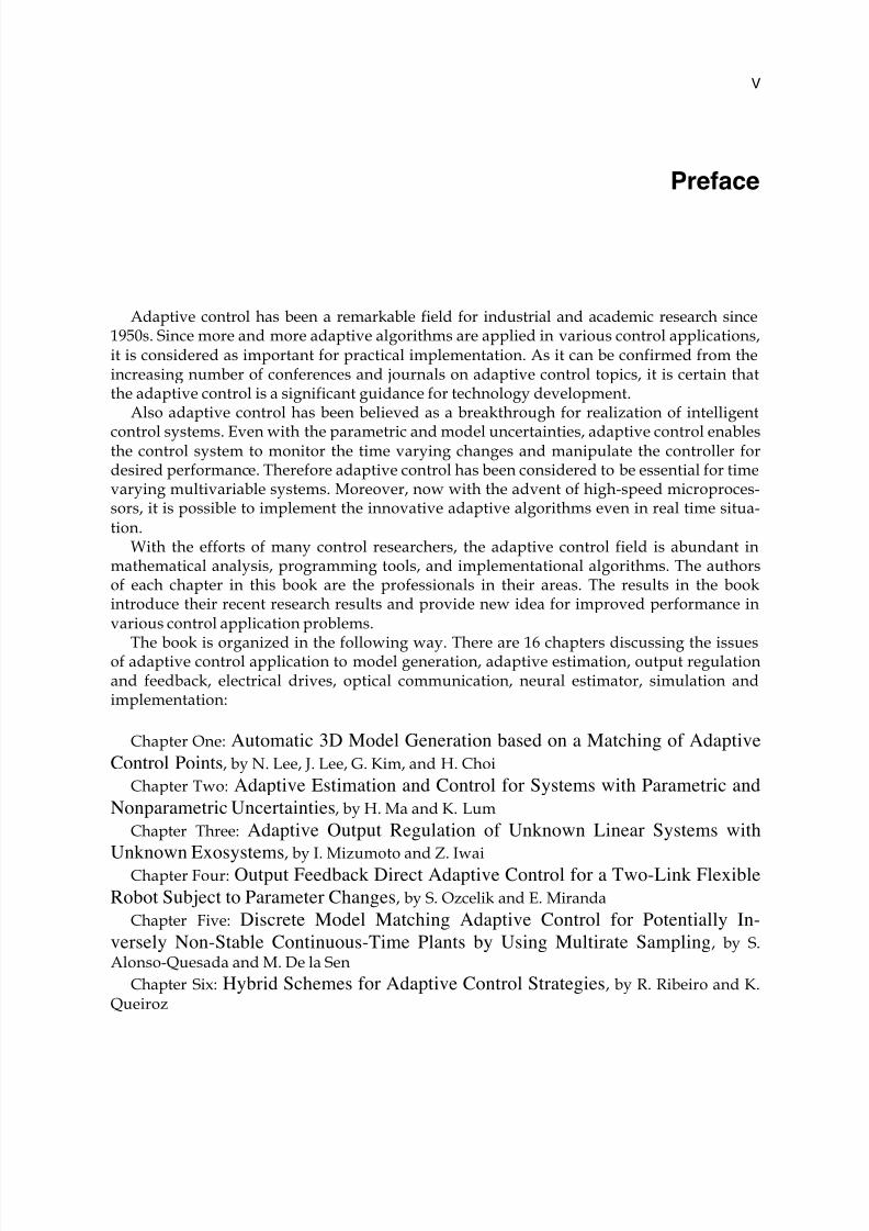
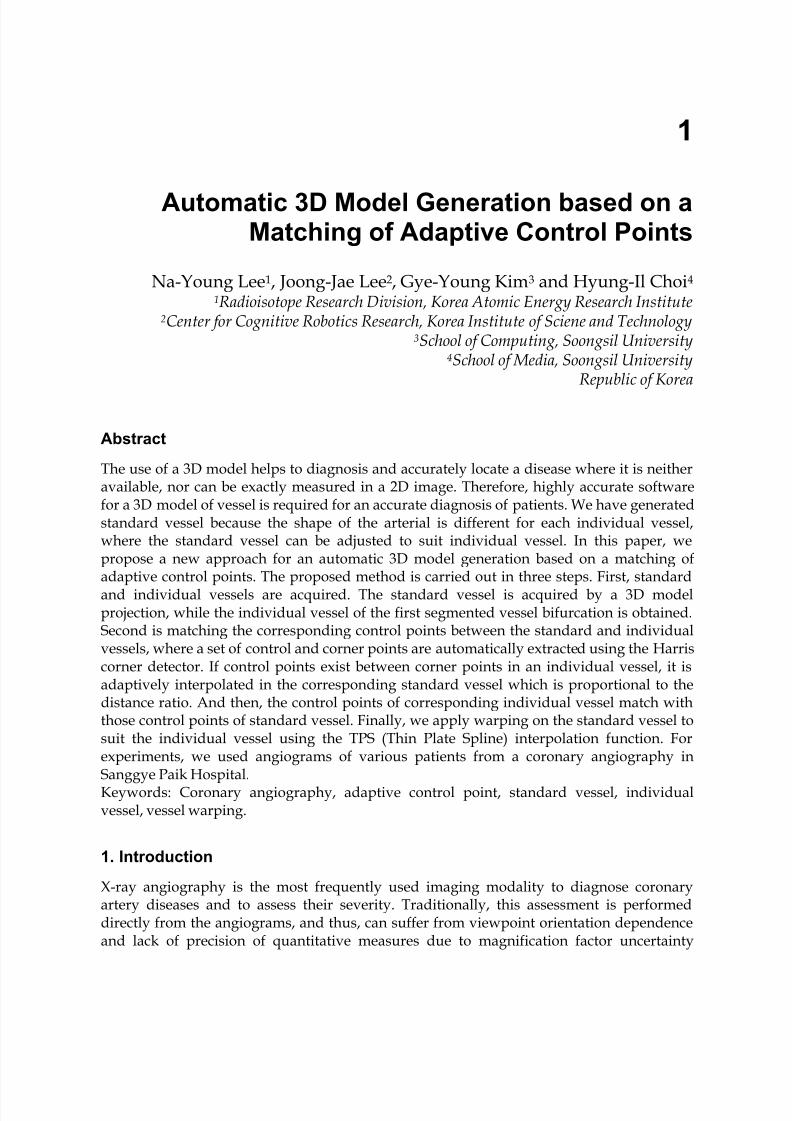
(Messenger et al., 2000), (Lee et al., 2006) and (Lee et al., 2007). 3D model is provided todisplay the morphology of vessel malformations such as stenoses, arteriovenousmalformations and aneurysms (Holger et al., 2005). Consequently, accurate software for a3D model of a coronary tree is required for an accurate diagnosis of patients. It could lead toa fast diagnosis and make it more accurate in an ambiguous condition.In this paper, we present an automatic 3D model generation based on a matching ofadaptive control points. Fig. 1 shows the overall flow of the proposed method for the 3Dmodelling of the individual vessel. The proposed method is composed as the followingthree steps: image acquisition, matching of the adaptive control points and the vesselwarping. In Section 2, the acquisitions of the input image in standard and individual vesselsare described. Section 3 presents the matching of the corresponding control points betweenthe standard and individual vessels. Section 4 describes the 3D modelling of the individualvessel which is performed through a vessel warping with the corresponding control points.Experimental results of the vessel transformation are given in Section 5. Finally, we presentthe conclusion in Section 6.
Fig. 1. Overall flow of the system configuration

Automatic 3D Model Generation based on a Matching of Adaptive Control Points 3
2. Image Acquisition
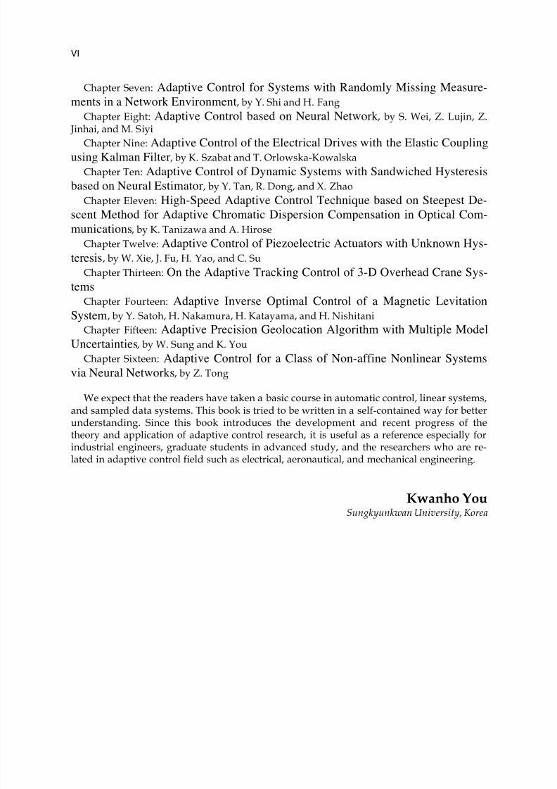
We have generated a standard vessel because the shape of the arterial is different for eachindividual vessel, where the standard vessel can be adjusted to suit the individual vessel(Chalopin et al., 2001), (Lee et al., 2006) and (Lee et al., 2007). The proposed approach isbased on a 3D model of standard vessel which is built from a database that implemented aKorean vascular system (Lee et al., 2006).We have limited the scope of the main arteries for the 3D model of the standard vessel asdepicted in Fig. 2.
Fig. 2. Vessel scope of the database for the 3D model of the standard vessel
Table 1 shows the database of the coronary artery of Lt. main (Left Main Coronary Artery),LAD (Left Anterior Descending) and LCX (Left Circumflex artery) information. Thisdatabase consists of 40 people with mixed gender information.
Lt. main LAD LCXage
Os distal length Os distal length Os distal length
below 60 years of
old (male)48.4±5.9 4.3±0.4 4.1±0.5 9.9±4.2 3.8±0.4 3.6±0.4 17.0±5.2 3.5±0.4 3.3±0.3 19.2±6.1
above 60 years of
old (male)67.5±5.4 4.5±0.5 4.4±0.4 8.4±3.8 3.9±0.3 3.6±0.3 17.2±5.8 3.6±0.4 3.4±0.4 24.6±8.9
below 60 years of
old (female)44.9±19.9 3.7±1.8 3.4±1.6 10.6±6.2 3.3±1.5 3.1±1.4 14.1±5.5 2.9±1.3 2.8±1.2 21.3±9.2
above 60 years of
old (female)70.7± 4.4 4.3±0.7 4.1±0.6 12.5±7.9 3.5±0.6 3.4±0.5 22.3±7.3 3.3±0.4 3.1±0.3 27.5±3.7
Table 1. Database of the coronary artery
Adaptive Control4
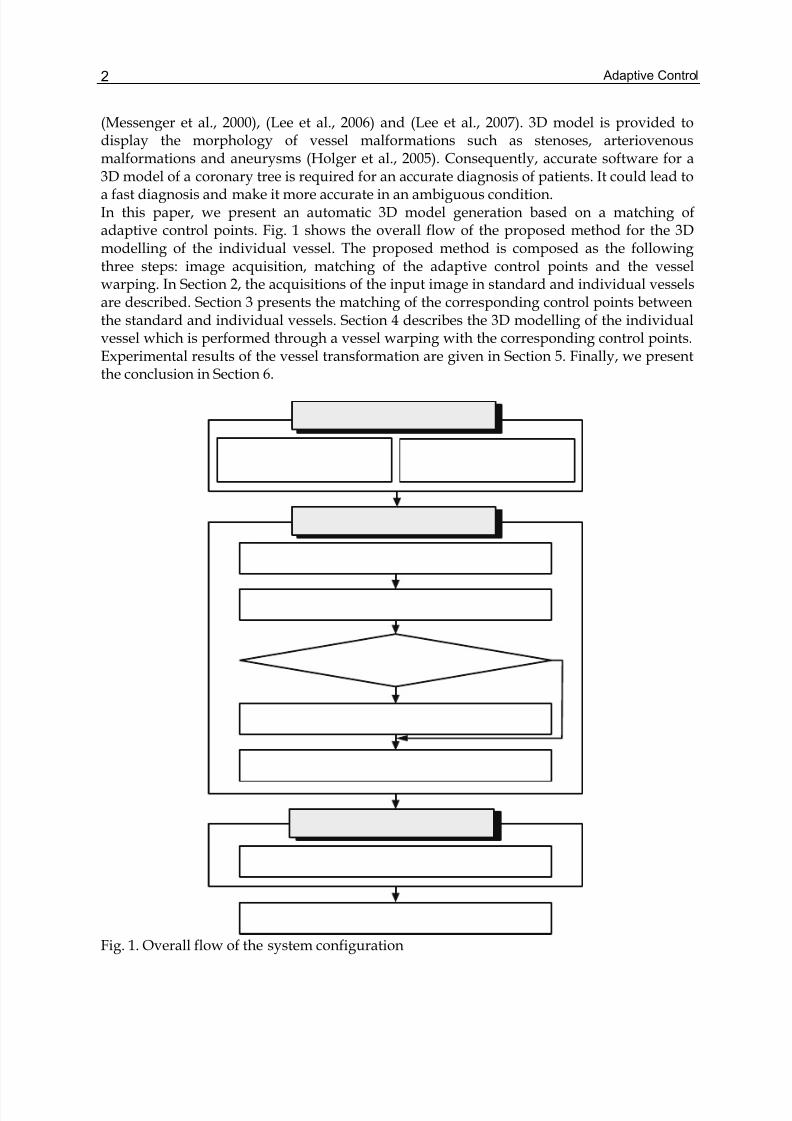
To quantify the 3D model of the coronary artery, the angles of the vessel bifurcation aremeasured with references to LCX, Lt. main and LAD, as in Table 2. Ten individualsregardless of their gender and age were selected randomly for measuring the angles of thevessel bifurcation from six angiograms. The measurement results, and the average andstandard deviations of each individual measurement are shown in Table 2.
RAO30°
CAUD30°
RAO30°CRA30°
AP0°CRA30°
LAO60°CRA30°
LAO60°CAUD30°
AP0°CAUD30°
1 69.17 123.31 38.64 61.32 84.01 50.98
2 53.58 72.02 23.80 51.75 99.73 73.92
3 77.28 97.70 21.20 57.72 100.71 71.33
4 94.12 24.67 22.38 81.99 75.6 69.57
5 64.12 33.25 31.24 40.97 135.00 61.87
6 55.34 51.27 41.8 80.89 119.84 57.14
7 71.93 79.32 50.92 87.72 114.71 58.22
8 67.70 59.14 31.84 58.93 92.36 70.16
9 85.98 60.85 35.77 54.45 118.80 78.93
10 47.39 60.26 34.50 47.39 67.52 34.79
Average 68.67 66.18 33.21 62.31 100.83 62.69
Standarddeviation
14.56 29.07 9.32 15.86 21.46 13.06
Table 2. Measured angles of the vessel bifurcation from six angiographies
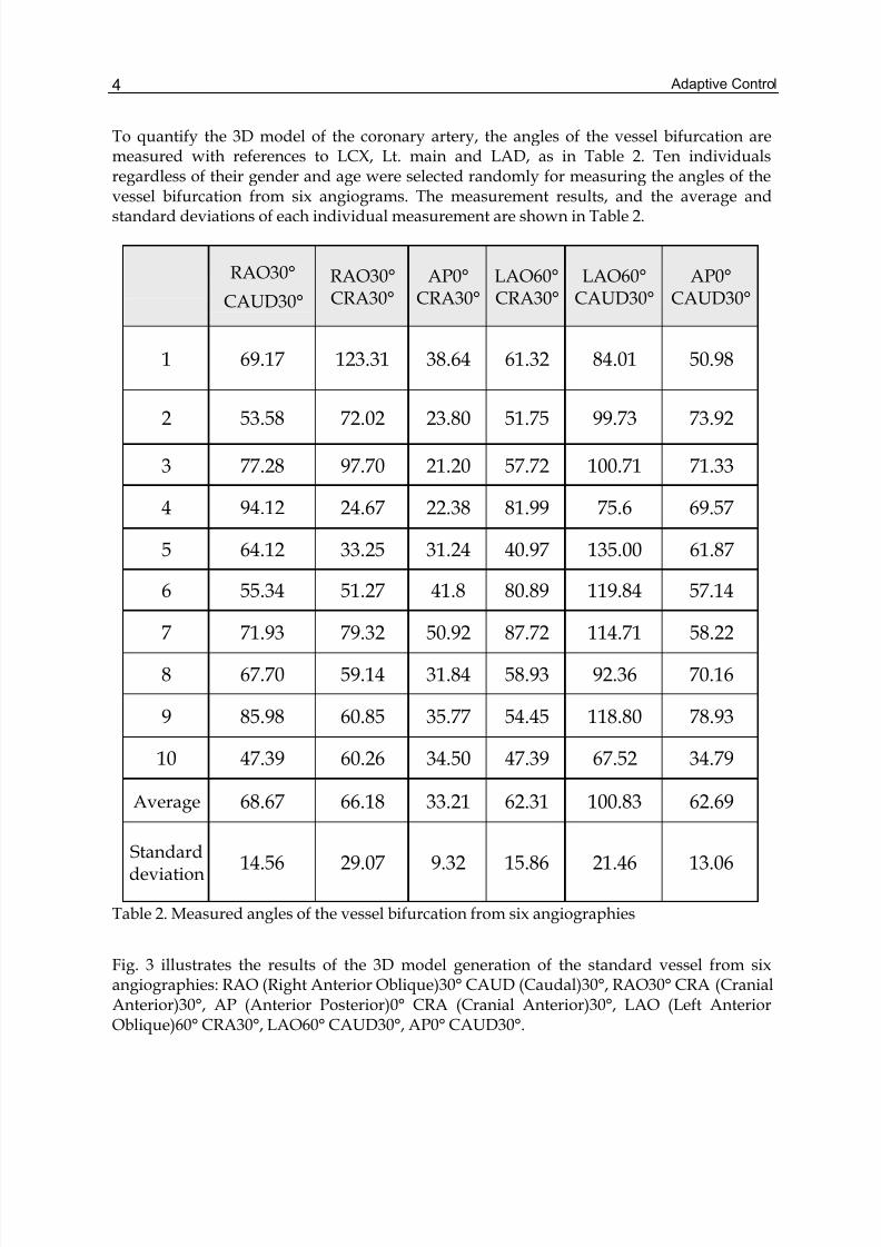
Fig. 3 illustrates the results of the 3D model generation of the standard vessel from sixangiographies: RAO (Right Anterior Oblique)30° CAUD (Caudal)30°, RAO30° CRA (CranialAnterior)30°, AP (Anterior Posterior)0° CRA (Cranial Anterior)30°, LAO (Left AnteriorOblique)60° CRA30°, LAO60° CAUD30°, AP0° CAUD30°.
Automatic 3D Model Generation based on a Matching of Adaptive Control Points 5
ViewRAO30°
CAUD30°RAO30°CRA30°
AP0°CRA30°
Angiogram
3D Model
ViewLAO60°CRA30°
LAO60°CAUD30°
AP0°CAUD30°
Angiogram
3D Model
Fig. 3. 3D model generation of the standard vessel from six angiographies
Evaluating the angles of the vessel bifurcation from six angiographies can reduce thepossible measurement error which occurs when the angle from a single view is measured.
Adaptive Control6
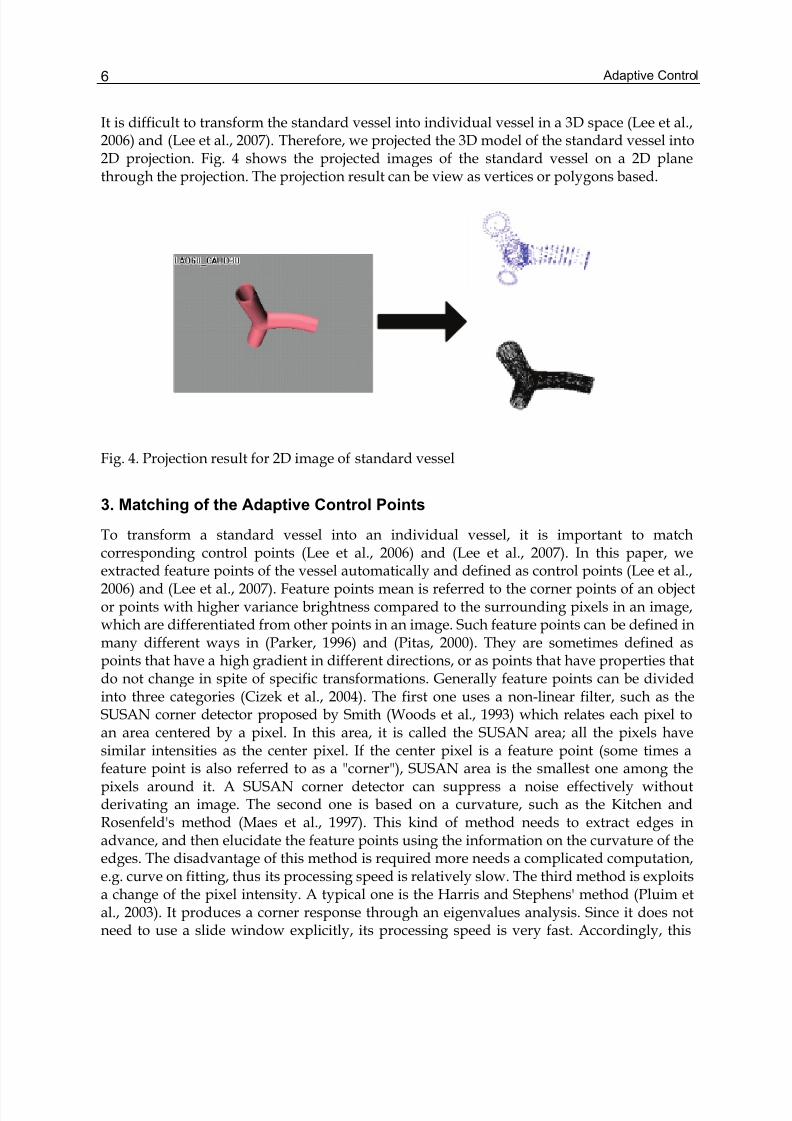
It is difficult to transform the standard vessel into individual vessel in a 3D space (Lee et al.,2006) and (Lee et al., 2007). Therefore, we projected the 3D model of the standard vessel into2D projection. Fig. 4 shows the projected images of the standard vessel on a 2D planethrough the projection. The projection result can be view as vertices or polygons based.
Fig. 4. Projection result for 2D image of standard vessel
3. Matching of the Adaptive Control Points
To transform a standard vessel into an individual vessel, it is important to matchcorresponding control points (Lee et al., 2006) and (Lee et al., 2007). In this paper, weextracted feature points of the vessel automatically and defined as control points (Lee et al.,2006) and (Lee et al., 2007). Feature points mean is referred to the corner points of an objector points with higher variance brightness compared to the surrounding pixels in an image,which are differentiated from other points in an image. Such feature points can be defined inmany different ways in (Parker, 1996) and (Pitas, 2000). They are sometimes defined aspoints that have a high gradient in different directions, or as points that have properties thatdo not change in spite of specific transformations. Generally feature points can be dividedinto three categories (Cizek et al., 2004). The first one uses a non-linear filter, such as theSUSAN corner detector proposed by Smith (Woods et al., 1993) which relates each pixel toan area centered by a pixel. In this area, it is called the SUSAN area; all the pixels havesimilar intensities as the center pixel. If the center pixel is a feature point (some times afeature point is also referred to as a "corner"), SUSAN area is the smallest one among thepixels around it. A SUSAN corner detector can suppress a noise effectively withoutderivating an image. The second one is based on a curvature, such as the Kitchen andRosenfeld's method (Maes et al., 1997). This kind of method needs to extract edges inadvance, and then elucidate the feature points using the information on the curvature of theedges. The disadvantage of this method is required more needs a complicated computation,e.g. curve on fitting, thus its processing speed is relatively slow. The third method is exploitsa change of the pixel intensity. A typical one is the Harris and Stephens' method (Pluim etal., 2003). It produces a corner response through an eigenvalues analysis. Since it does notneed to use a slide window explicitly, its processing speed is very fast. Accordingly, this
Automatic 3D Model Generation based on a Matching of Adaptive Control Points 7
paper used the Harris corner detector to find the control points of standard and individualvessels (Lee et al., 2006) and (Lee, 2007).
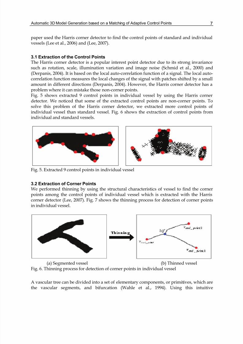
3.1 Extraction of the Control PointsThe Harris corner detector is a popular interest point detector due to its strong invariancesuch as rotation, scale, illumination variation and image noise (Schmid et al., 2000) and(Derpanis, 2004). It is based on the local auto-correlation function of a signal. The local auto-correlation function measures the local changes of the signal with patches shifted by a smallamount in different directions (Derpanis, 2004). However, the Harris corner detector has aproblem where it can mistake those non-corner points.Fig. 5 shows extracted 9 control points in individual vessel by using the Harris cornerdetector. We noticed that some of the extracted control points are non-corner points. Tosolve this problem of the Harris corner detector, we extracted more control points ofindividual vessel than standard vessel. Fig. 6 shows the extraction of control points fromindividual and standard vessels.
Fig. 5. Extracted 9 control points in individual vessel
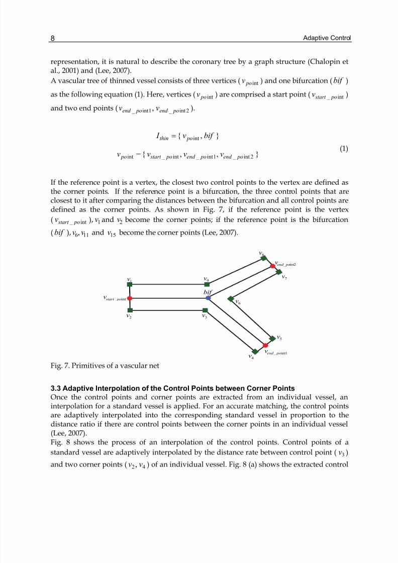
3.2 Extraction of Corner PointsWe performed thinning by using the structural characteristics of vessel to find the cornerpoints among the control points of individual vessel which is extracted with the Harriscorner detector (Lee, 2007). Fig. 7 shows the thinning process for detection of corner pointsin individual vessel.
(a) Segmented vessel (b) Thinned vesselFig. 6. Thinning process for detection of corner points in individual vessel
A vascular tree can be divided into a set of elementary components, or primitives, which arethe vascular segments, and bifurcation (Wahle et al., 1994). Using this intuitive
Adaptive Control8
representation, it is natural to describe the coronary tree by a graph structure (Chalopin etal., 2001) and (Lee, 2007).
A vascular tree of thinned vessel consists of three vertices ( int pov ) and one bifurcation (bif )
as the following equation (1). Here, vertices ( int pov ) are comprised a start point ( int _ po start v )
and two end points ( 2int _ 1int _ , poend poend vv ).
, int bif v I pothin =
,, 2int _ 1int _ int _ int poend poend po start po vvvv = (1)
If the reference point is a vertex, the closest two control points to the vertex are defined asthe corner points. If the reference point is a bifurcation, the three control points that areclosest to it after comparing the distances between the bifurcation and all control points aredefined as the corner points. As shown in Fig. 7, if the reference point is the vertex
( int _ po start v ), 1v and 2v become the corner points; if the reference point is the bifurcation
( bif ), 116, vv and 15v become the corner points (Lee, 2007).
int _ po start v
1int _ poend v
bif
2int _ poend v
1v 9v
8v
7v
6v
5v
4v
3v2v
Fig. 7. Primitives of a vascular net
3.3 Adaptive Interpolation of the Control Points between Corner Points
Once the control points and corner points are extracted from an individual vessel, aninterpolation for a standard vessel is applied. For an accurate matching, the control pointsare adaptively interpolated into the corresponding standard vessel in proportion to thedistance ratio if there are control points between the corner points in an individual vessel(Lee, 2007).Fig. 8 shows the process of an interpolation of the control points. Control points of a
standard vessel are adaptively interpolated by the distance rate between control point ( 3v )
and two corner points ( 42, vv ) of an individual vessel. Fig. 8 (a) shows the extracted control
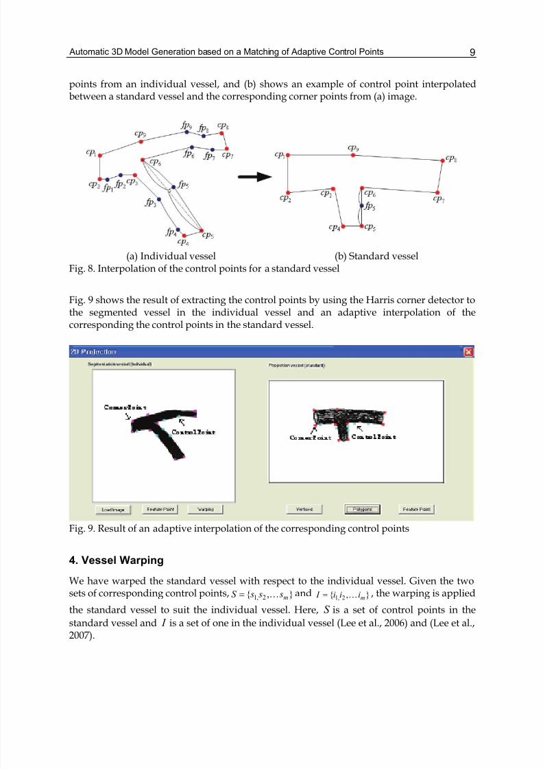
Automatic 3D Model Generation based on a Matching of Adaptive Control Points 9
points from an individual vessel, and (b) shows an example of control point interpolatedbetween a standard vessel and the corresponding corner points from (a) image.
(a) Individual vessel (b) Standard vesselFig. 8. Interpolation of the control points for a standard vessel
Fig. 9 shows the result of extracting the control points by using the Harris corner detector tothe segmented vessel in the individual vessel and an adaptive interpolation of thecorresponding the control points in the standard vessel.
Fig. 9. Result of an adaptive interpolation of the corresponding control points
4. Vessel Warping
We have warped the standard vessel with respect to the individual vessel. Given the twosets of corresponding control points, , 2,1 m s s sS K= and , 2,1 miii I K= , the warping is applied
the standard vessel to suit the individual vessel. Here, S is a set of control points in the
standard vessel and I is a set of one in the individual vessel (Lee et al., 2006) and (Lee et al.,2007).
Adaptive Control10
Standard vessel warping was performed using the TPS (Thin-Plate-Spline) algorithm(Bentoutou et al., 2002) from the two sets of control points.The TPS is the interpolation functions that exactly represent a distortion at each featurepoint, and for defining a minimum curvature surface between control points. A TPSfunction is a flexible transformation that allows for a rotation, translation, scaling, andskewing. It also allows for lines to bend according by the TPS model (Bentoutou et al., 2002).Therefore, a large number of deformations can be characterized by the TPS model.The TPS interpolation function can be written as equation (2).
∑=
−++=m
i
ii x x K W t Ax xh1
||)(||)( (2)
The variables A and t are the affine transformation parameters matrices, iW are the weights
of the non-linear radial interpolation functionK , and i x are the control points. The function
)(r K is the solution of the biharmonic equation )0( 2=Δ K that satisfies the condition of a
bending energy minimization, namely )(log)( 22 r r r K = .
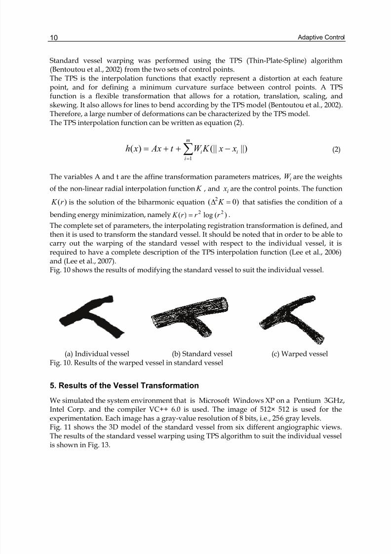
The complete set of parameters, the interpolating registration transformation is defined, andthen it is used to transform the standard vessel. It should be noted that in order to be able tocarry out the warping of the standard vessel with respect to the individual vessel, it isrequired to have a complete description of the TPS interpolation function (Lee et al., 2006)and (Lee et al., 2007).Fig. 10 shows the results of modifying the standard vessel to suit the individual vessel.
(a) Individual vessel (b) Standard vessel (c) Warped vesselFig. 10. Results of the warped vessel in standard vessel
5. Results of the Vessel Transformation
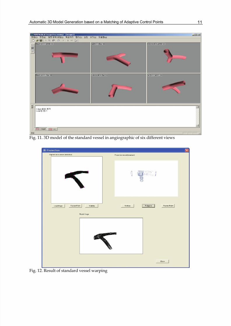
We simulated the system environment that is Microsoft Windows XP on a Pentium 3GHz, Intel Corp. and the compiler VC++ 6.0 is used. The image of 512× 512 is used for theexperimentation. Each image has a gray-value resolution of 8 bits, i.e., 256 gray levels.Fig. 11 shows the 3D model of the standard vessel from six different angiographic views.The results of the standard vessel warping using TPS algorithm to suit the individual vesselis shown in Fig. 13.
Automatic 3D Model Generation based on a Matching of Adaptive Control Points 11
Fig. 11. 3D model of the standard vessel in angiographic of six different views
Fig. 12. Result of standard vessel warping

Adaptive Control12
Fig. 13 shows the result for an automatically 3D model generation of individual vessel.
Fig. 13. Result of 3D model generation for the individual vessel in six views
6. Conclusion
We proposed a fully automatic and effective algorithm to perform a 3D modelling ofindividual vessel from angiograms in six views. This approach can be used to recover thegeometry of the main arteries. The 3D model of the vessel enables patients to visualize theirprogress and improvement for a disease. Such a model should not only enhance the level ofreliability but also provide a fast and accurate identification. In order words, this methodcan be expected to reduce the number of misdiagnosed cases (Lee et al., 2006) and (Lee et al.,2007).
7. Acknowledgement
“This Work was supported by Soongsil University and Korea Research Foundation Grant(KRF-2006-005-J03801) Funded by Korean Government.”
8. References
A, Venot.; J.F, Lebruchec. & J.C, Roucayrol. (1984). A new class of similarity measures forrobust image registration, Comput. Vision Graph. Image Process, pp. 176-184.
Automatic 3D Model Generation based on a Matching of Adaptive Control Points 13
A, Wahle.; E, Wellnhofer.; I, Mugaragu.;H.U, Sauer.; H, Oswald. & E, Fleck. (1994). Accurate3-D reconstruction and statistics for assessment of diffuse coronary artery disease,Computers in Cardiology, IEEE Computer Society, Los Alamitos, CA, pp.669-672
B.G, Brown.; E, Bolson.; M, Frimer. & H, Dodge. (1977). Quantitative coronary arteriographyestimation of dimensions, hemodynamic resistance, and atheroma mass ofcoronary artery lesions using the arteriogram and digital computation, Circulation,vol. 55, pp. 329-337
C, Blondel.; R, Vaillant.; F, Devernary. ; G, Malandain. & N, Ayache. (2002). Automatictrinocular 3D reconstruction of coronary artery centerlines from rotational X-rayangiography, Computer Assisted Radiology and Surgery 2002 Proceedings, Paris, June2002, Springer Publishers, Heidelberg
Claire, Chalopin.; Gerard, Finet. & Isabelle E, Magnin. (2001). Modeling the 3D coronary treefor labeling purposes. Medical Image Analysis, pp.301-315
Chris, Harris. & Mike, Stephens. (1988). A combined corner and edge detector, Proceedings of the Fourth Alvey Vision Conference, pp.147-151, Manchester
C, Lorenz.; S, Renisch.; S, Schlatholter. & T, Bulow. (2003). Simultaneous Segmentation andTree Reconstruction of the Coronary Arteries in MSCT Images , Int. Symposium Medical Imaging, San Diego, Proc. SPIE Vol. 5032, pp. 167-177
C, Schmid.; R, Mohr. & C, Bauckhage. (2000). Evaluation of interest point detectors.International Journal of Computer Vision, pp. 151-172
F.L, Bookstein. (1989). Principal warps: thin-plate splines and the decomposition ofdeformations, IEEE-PAMI 11, pp. 567-585
F, Maes.; A, Collignon.; G, Marchal. & P, Suetens. (1997). Multimodality image registrationby maximization of mutual information, IEEE Transaction on Medical Imaging, Vol.16, No. 2, pp.187-198
Holger, Schmitt.; Michael, Grass.; Rolf, Suurmond.; Thomas Kohler.; Volker, Rasche.; Stefan,Hahnel. & Sabine, Heiland. (2005). Reconstruction of blood propagation in three-dimensional rotational X-ray angiography. Computerized Medical Imaging andGraphics, 29, pp. 507-520
I, Pitas. (2000). Digital image processing algorithms and applications, 1st Ed., John Wiley & Sons,Inc., ISBN 0471377392, New York
J.C, Messenger.; S.Y,Chen.; J.D, Carroll.; J.E, Burchenal.; K, Kioussopoulos. & B.M, Groves.(2000). 3D coronary reconstruction from routine single-place coronary angiograms:clinical validation and quantitative analysis of the right coronary artery in 100patients, The International Journal of Cardiac Imaging 16(6), pp.413-427
J, Cizek.; K, Herholz.; S, Vollmar.; R, Schrader.; J, Klein. & W.D, Heiss. (2004). Fast androbust registration of PET and MR image of human brin, Neuroimage, Vol. 22, Iss.1, pp.434-442
J, Flusser. & T,Suk. (1998). Degraded image analysis: an invariant approach , IEEE Trans.Pattern Anal. Mach. Intell, pp. 590-603
Jianbo, Shi. & Carlo, Tomasi. (1994). Good features to track, IEEE Conference on CVPR Seattle,pp. 593-600
J.P.W, Pluim.; J.B.A, Maintz. & M.A, Viergever. (2003). Mutual information basedregistration of medical images: a survey, IEEE Transactions on Medical Imaging,Vol. 22, No. 8, pp. 986-1004
Adaptive Control14
J.R, Parker. (1996). Algorithms for image processing and computer vision, 1st Ed., John Wiley &Sons, Inc., IBSN 0471140562, USA
J, Ross. et al. (1987). Guidelines for coronary angiography,Circulation, vol.76K, Derpanis. (2004). The Harris corner detectorM, Grass.; R, Koppe.; E, Klotz.; R, Proksa.; MH, Kuhn.; H, Aerts. & etc (1999). 3D
reconstruction of high contrast objects using C-arm image intensifier projectiondata, Computer Med Imaging Graphics, 23(6):311-321
M, Grass.; R, Koppe.; E, Klotz.; Op de Beek J. & R, Kemkers. (1999). 3D reconstruction andimaging based on C-arm systems, Med Biol Eng Comput, 37(2):1520-1
M, Grass.; R, Guillemaud.; R, Koppe.; E, Klotz.; V, Rasche. & Op de Beek J. (2002). Laradiologie tridimensionelle, La tomography medicale-imagerie morphologique et imagerie fonctionelle, Hermes Science Publications, Paris
Na-Young, Lee.; Gye-Young, Kim. & Hyung-Il, Choi. (2006). Automatic generationtechnique of three-dimensional model corresponding to individual vessels,Computational Science and Its Applications-ICCSA 2006, LNCS 3984, PP.441-449,Glasgow, UK, May 2006, Springer-Verlag Berlin Heidelberg
Na-Young, Lee. (2006). An automatic generating technique of individual vessels based ongeneral vessels, The 7 th International Workshop on Image Analysis for MultimediaInteractive Services, pp.241-244, Korea, April, 2006, Incheon
NaYoung, Lee.; JeongHee, Cha.; JinWook, On.; GyeYoung, Kim. & HyungIl, Choi. (2006).An automatic generation technique of 3D vessels model form angiograms,Proceedings of The 2006 International Conference on Image Processing, Computer Vision,& Pattern Recognition, pp.371-376, USA, June, 2006, CSREA Press, Las Vegas
Na-Young, Lee. (2007). Automatic generation of 3D vessels model using vessels imagematching based on adaptive control points, Sixth International Conference on Advanced Language Processing and Web Information Technology, pp.265-270, ISBN 0-7695-2930-5, China, August 2007, IEEE Computer Society, Luoyang, Henan
Na-Young, Lee.; Gye-Young, Kim. & Hyung-Il, Choi. (2007). 3D modelling of the vesselsfrom X-ray angiography, Digital Human Modeling, HCII 2007 , LNCS 4561, pp.646-654, IBSN 978-3-540-73318-8 , Springer Berlin Heidelberg
Na-Young, Lee.; Gye-Young, Kim. & Hyung-Il, Choi. (2007). 3D model of vessels fromangiograms, Proceedings of the 13th Japan-Korea join workshop on frontiers of computer vision, pp.235-240, Korea, January 2007, Busan
Na-Young, Lee. (2007). Three Dimensional Modeling of Individual Vessels Based onMatching of Adaptive Control Points, MICAI 2007: Advances in Artificial Intelligence,LNAI 4827, pp. 1143–1150, Springer-Verlag Berlin Heidelberg
P, de Feyter.; J, Vos.; J, Reiber. & P, Serruys. (1993). Value and limitations of quantitativecoronary angiography to assess progression and regression of coronaryatherosclerosis. In Advances in Quantitative Coronary Arteriography, pp. 255-271
R.P, Woods.; J.C, Mazziotta. & S.R, Cherry. (1993). MRI-PET registration with automatedalgorithm, Journal of computer assisted tomography. Vol. 17:44, pp.536-546
Y, Bentoutou.; N, Taleb.; M, Chikr El Mezouar, M, Taleb. & L, Jetto. (2002). An invariantapproach for image registration in digital subtraction angiography. PatternRecognition, Vol. 35, Iss. 12, December 2002, pp. 2853-2865
2
Adaptive Estimation and Control for Systemswith Parametric and
Nonparametric Uncertainties
Hongbin Ma* and Kai-Yew Lum† Temasek Laboratories, National University of Singapore
[email protected]* [email protected]†
Abstract
Adaptive control has been developed for decades, and now it has become a rigorous andmature discipline which mainly focuses on dealing parametric uncertainties in controlsystems, especially linear parametric systems. Nonparametric uncertainties were seldomstudied or addressed in the literature of adaptive control until new areas on exploringlimitations and capability of feedback control emerged in recent years. Comparing with theapproach of robust control to deal with parametric or nonparametric uncertainties, theapproach of adaptive control can deal with relatively larger uncertainties and gain moreflexibility to fit the unknown plant because adaptive control usually involves adaptiveestimation algorithms which play role of “learning” in some sense.This chapter will introduce a new challenging topic on dealing with both parametric andnonparametric internal uncertainties in the same system. The existence of both two kinds ofuncertainties makes it very difficult or even impossible to apply the traditional recursiveidentification algorithms which are designed for parametric systems. We will discuss byexamples why conventional adaptive estimation and hence conventional adaptive controlcannot be applied directly to deal with combination of parametric and nonparametricuncertainties. And we will also introduce basic ideas to handle the difficulties involved inthe adaptive estimation problem for the system with combination of parametric andnonparametric uncertainties. Especially, we will propose and discuss a novel class ofadaptive estimators, i.e. information-concentration (IC) estimators. This area is still in its infantstage, and more efforts are expected in the future for gainning comprehensiveunderstanding to resolve challenging difficulties.Furthermore, we will give two concrete examples of semi-parametric adaptive control todemonstrate the ideas and the principles to deal with both parametric and nonparametricuncertainties in the plant. (1) In the first example, a simple first-order discrete-time nonlinearsystem with both kinds of internal uncertainties is investigated, where the uncertainty ofnon-parametric part is characterized by a Lipschitz constant L, and the nonlinearity ofparametric part is characterized by an exponent index b. In this example, based on the ideaof the IC estimator, we construct a unified adaptive controller in both cases of b = 1 and
Adaptive Control16
b > 1, and its closed-loop stability is established under some conditions. When theparametric part is bilinear (b = 1), the conditions given reveal the magic number
22
3+ which appeared in previous study on capability and limitations of the feedback
mechanism. (2) In the second example with both parametric uncertainties and non-parametric uncertainties, the controller gain is also supposed to be unknown besides theunknown parameter in the parametric part, and we only consider the noise-free case. For thismodel, according to some a priori knowledge on the non-parametric part and the unknowncontroller gain, we design another type of adaptive controller based on a gradient-likeadaptation law with time-varying deadzone so as to deal with both kinds of uncertainties.And in this example we can establish the asymptotic convergence of tracking error undersome mild conditions, althouth these conditions required are not as perfect as in the first
example in sense that L < 0.5 is far away from the best possible bound 22
3+ .
These two examples illustrate different methods of designing adaptive estimation andcontrol algorithms. However, their essential ideas and principles are all based on the a priori knowledge on the system model, especially on the parametric part and the non-parametric part. From these examples, we can see that the closed-loop stability analysis israther nontrivial. These examples demonstrate new adaptive control ideas to deal with twokinds of internal uncertainties simultaneously and illustrates our elementary theoreticalattempts in establishing closed-loop stability.
1. Introduction
This chapter will focus on a special topic on adaptive estimation and control for systems withparametric and nonparametric uncertainties. Our discussion on this topic starts with a verybrief introduction to adaptive control.
1.1 Adaptive Control
As stated in [SB89], “Research in adaptive control has a long and vigorous history” sincethe initial study in 1950s on adaptive control which was motivated by the problem ofdesigning autopilots for air-craft operating at a wide range of speeds and altitudes. Withdecades of efforts, adaptive control has become a rigorous and mature discipline whichmainly focuses on dealing parametric uncertainties in control systems, especially linearparametric systems.From the initial stage of adaptive control, this area has been aiming at study how to dealwith large uncertainties in control systems. This goal of adaptive control essentially meansthat one adaptive control law cannot be a fixed controller with fixed structure and fixedparameters because any fixed controller usually can only deal with small uncertainties incontrol systems. The fact that most fixed controllers with certain structure (e.g. linearfeedback control) designed for an exact system model (called nominal model) can also workfor a small range of changes in the system parameter is often referred to as robustness,which is the kernel concept of another area, robust control. While robust control focuses onstudying the stability margin of fixed controllers (mainly linear feedback controller), whose
Adaptive Estimation and Control for Systems with Parametric and Nonparametric Uncertainties 17
design essentially relies on priori knowledge on exact nominal system model and boundsof uncertain parameters, adaptive control generally does not need a priori informationabout the bounds on the uncertain or (slow) time-varying parameters. Briefly speaking,comparing with the approach of robust control to deal with parametric or nonparametricuncertainties, the approach of adaptive control can deal with relatively larger uncertaintiesand gain more flexibility to fit the unknown plant because adaptive control usuallyinvolves adaptive estimation algorithms which play role of “learning” in some sense.The advantages of adaptive control come from the fact that adaptive controllers can adaptthemselves to modify the control law based on estimation of unknown parameters byrecursive identification algorithms. Hence the area of adaptive control has close connectionswith system identification, which is an area aiming at providing and investigatingmathematical tools and algorithms that build dynamical models from measured data.Typically, in system identification, a certain model structure is chosen by the user whichcontains unknown parameters and then some recursive algorithms are put forward basedon the structural features of the model and statistical properties of the data or noise. Themethods or algorithms developed in system identification are borrowed in adaptive controlin order to estimate the unknown parameters in the closed loop. For convenience, theparameter estimation methods or algorithms adopted in adaptive control are oftenreferred to as adaptive estimation methods. Adaptive estimation and system identificationshare many similar characteristics, for example, both of them originate and benefit fromthe development of statistics. One typical example is the frequently used least-squares (LS)algorithm, which gives parameter estimation by minimizing the sum of squared errors (orresiduals), and we know that LS algorithm plays important role in many areas includingstatistics, system identification and adaptive control. We shall also remark that, in spite ofthe significant similarities and the same origin, adaptive estimation is different fromsystem identification in sense that adaptive estimation serves for adaptive control anddeals with dynamic data generated in the closed loop of adaptive controller, which meansthat statistical properties generally cannot be guaranteed or verified in the analysis ofadaptive estimation. This unique feature of adaptive estimation and control brings manydifficulties in mathematical analysis, and we will show such difficulties in later examplesgiven in this paper.
1.2 Linear Regression Model and Least Square Algorithm
Major parts in existing study on regression analysis (a branch of statistics) [DS98, Ber04,Wik08j], time series analysis [BJR08, Tsa05], system identification [Lju98, VV07] andadaptive control [GS84, AW89, SB89, CG91, FL99] center on the following linear regressionmodel
k k k v z += φ θ τ (1)
where k z , k φ , k v represent observation data, regression vector and noise disturbance (or
external uncertainties), respectively. Here θ is the unknown parameter to be estimated.Linear regression models have many applications in many disciplines of science andengineering [Wik08g, web08, DS98, Hel63, Wei05, MPV07, Fox97, BDB95]. For example, as
Adaptive Control18
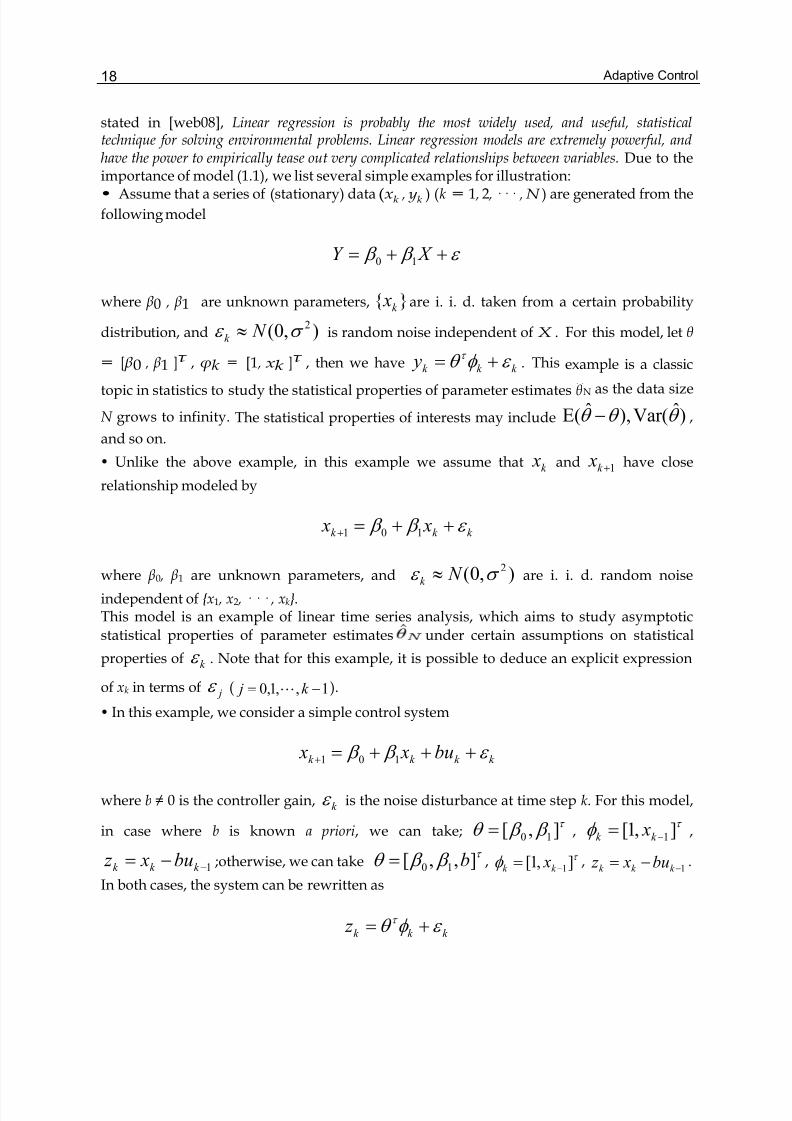
stated in [web08], Linear regression is probably the most widely used, and useful, statisticaltechnique for solving environmental problems. Linear regression models are extremely powerful, andhave the power to empirically tease out very complicated relationships between variables. Due to theimportance of model (1.1), we list several simple examples for illustration:• Assume that a series of (stationary) data (xk , yk ) (k = 1 , 2 , · · · , N ) are generated from the
following model
ε β β ++= X Y 10
where β0 , β1 are unknown parameters, k x are i. i. d. taken from a certain probability
distribution, and ),0( 2σ ε N k ≈ is random noise independent of X . For this model, let θ
= [ β0 , β1 ]τ , φk = [1 , xk ]τ , then we have k k k y ε φ θ τ += . This example is a classic
topic in statistics to study the statistical properties of parameter estimates θN as the data size
N grows to infinity. The statistical properties of interests may include )ˆVar(),ˆE( θ θ θ − ,
and so on.
• Unlike the above example, in this example we assume that k x and 1+k x have close
relationship modeled by
k k k x x ε β β ++=+ 101
where β0 , β1 are unknown parameters, and ),0( 2σ ε N k ≈ are i. i. d. random noise
independent of x1 , x2 , · · · , xk .This model is an example of linear time series analysis, which aims to study asymptotic
statistical properties of parameter estimates under certain assumptions on statistical
properties of k ε . Note that for this example, it is possible to deduce an explicit expression
of xk in terms of jε ( 1,,1,0 −= k j L ).
• In this example, we consider a simple control system
k k k k bu x x ε β β +++=+ 101
where b ≠ 0 is the controller gain, k ε is the noise disturbance at time step k. For this model,
in case where b is known a priori, we can take;τ β β θ ],[ 10= ,
τ φ ],1[ 1−= k k x ,
1−−= k k k bu x z ;otherwise, we can takeτ β β θ ],,[ 10 b= , τ φ ],1[ 1−= k k x ,
1−−= k k k bu x z .
In both cases, the system can be rewritten as
k k k z ε φ θ τ +=
Adaptive Estimation and Control for Systems with Parametric and Nonparametric Uncertainties 19
which implies that intuitively, θ can be estimated by using the identification algorithm since
both data zk andk φ are available at time step k. Let
k θ denote the parameter estimates at
time stepk θ , then we can design the control signal
k u by regarding as the real parameter
θ:
where k r is the known reference signal to be tracked, and b , 0ˆ β , 1
ˆ β are estimates of b ,
0 β , 1 β , respectively. Note that for this example, the closed-loop system will be very
complex because the data generated in the closed loop essentially depend on all historysignals. In the closed-loop system of an adaptive controller, generally it is difficult toanalyze or verify statistical properties of signals, and this fact makes that adaptiveestimation and control cannot directly employ techniques or results from systemidentification. Now we briefly introduce the frequently-used LS algorithm for model (1.1)due to its importance and wide applications [LH74, Gio85, Wik08e, Wik08f, Wik08d]. Theidea of LS algorithm is simply to minimize the sum of squared errors, that is to say,
(1.2)
This idea has a long history rooted from great mathematician Carl Friedrich Gauss in 1795and published first by Legendre in 1805. In 1809, Gauss published this method in volumetwo of his classical work on celestial mechanics, heoria Motus Corporum Coelestium insectionibus conicis solem ambientium[Gau09], and later in 1829, Gauss was able to state that theLS estimator is optimal in the sense that in a linear model where the errors have a mean ofzero, are uncorrelated, and have equal variances, the best linear unbiased estimators of thecoefficients is the least-squares estimators. This result is known as the Gauss-Markovtheorem [Wik08a].By Eq. (1.2), at every time step, we need to minimize the sum of squared errors, whichrequires much computation cost. To improve the computational efficiency, in practice weoften use the recursive form of LS algorithm, often referred to as recursive LS algorithm,which will be derived in the following. First, introducing the following notations
(1.3)
and using Eq. (1.1), we obtain that
Adaptive Control20
Noting that
where the last equation is derived from properties of Moore-Penrose pseudoinverse[Wik08h]
we know that the minimum of ][][ ς ς τ nnnn Z Z Φ−Φ− can be achieved at
(1.4)
which is the LS estimate of θ. Let
and then, by Eq. (1.3), with the help of matrix inverse identity
we can obtain that
111
1
1
1
1
1111
11111
11
1
)()]()(1)[(
][
)(
−−−
−
−
−
−
−−−−
−−−−−
−−
−
−=
+−=
+=
+=
nnnnnn
nnnnnnnnnn
nnnn
P P a P
P P P P P P
BAC B A A
P P
τ
τ τ
τ
τ
φ φ
φ φ φ φ
φ φ
where
Further,
Adaptive Estimation and Control for Systems with Parametric and Nonparametric Uncertainties 21
Thus, we can obtain the following recursive LS algorithm
where Pn−1 and θn−1 reflect only information up to step n − 1, while an,nφ and 1−− nnn z θ φ τ τ
reflect information up to step n. In statistics, besides linear parametric regression, there also exist generalized linear models[Wik08b] and non-parametric regression methods [Wik08i], such as kernel regression[Wik08c]. Interested readers can refer to the wiki pages mentioned above and the referencestherein.
1.3 Uncertainties and Feedback MechanismBy the discussions above, we shall emphasize that, in a certain sense, linear regressionmodels are kernel of classical (discrete-time) adaptive control theory, which focuses to copewith the parametric uncertainties in linear plants. In recent years, parametric uncertaintiesin nonlinear plants have also gained much attention in the literature[MT95, Bos95, Guo97,ASL98, GHZ99, LQF03]. Reviewing the development of adaptive control, we find thatparametric uncertainties were of primary interests in the study of adaptive control, nomatter whether the considered plants are linear or nonlinear. Nonparametric uncertaintieswere seldom studied or addressed in the literature of adaptive control until some new areason understanding limitations and capability of feedback control emerged in recent years.Here we mainly introduce the work initiated by Guo, who also motivated the authors’exploration in the direction which will be discussed in later parts.Guo’s work started from trying to understand fundamental relationship between theuncertainties and the feedback control. Unlike traditional adaptive theory, which focuses oninvestigating closed-loop stability of certain types of adaptive controllers, Guo began tothink over a general set of adaptive controllers, called feedback mechanism, i.e., all possiblefeedback control laws. Here the feedback control laws need not be restricted in a certainclass of controllers, and any series of mappings from the space of history data to the space ofcontrol signals is regarded as a feedback control law. With this concept in mind, since themost fundamental concept in automatic control, feedback, aims to reduce the effects of the
Adaptive Control22
plant uncertainty on the desired control performance, by introducing the set F of internaluncertainties in the plant and the whole feedback mechanism U , we wonder the followingbasic problems:1. Given an uncertainty set F , does there exist any feedback control law in U which canstabilize the plant? This question leads to the problem of how to characterize the maximumcapability of feedback mechanism.2. If the uncertainty set F is too large, is it possible that any feedback control law in U cannotstabilize the plant? This question leads to the problem of how to characterize the limitationsof feedback mechanism.
The philosophical thoughts to these problems result in fruitful study [Guo97, XG00, ZG02,XG01, LX06, Ma08a, Ma08b].The first step towards this direction was made in [Guo97], where Guo attempted to answerthe following question for a nontrivial example of discrete-time nonlinear polynomial plantmodel with parametric uncertainty: What is the largest nonlinearity that can be dealt withby feedback? More specifically, in [Guo97], for the following nonlinear uncertain system
(1.5)
where θ is the unknown parameter, b characterizes the nonlinear growth rate of the
system, and t w is the Gaussian noise sequence, a critical stability result is found — system
(1.5) is not a.s. globally stabilizable if and only if b ≥ 4. This result indicates that there existlimitations of the feedback mechanism in controlling the discrete-time nonlinear adaptivesystems, which is not seen in the corresponding continuous-time nonlinear systems (see[Guo97, Kan94]). The “impossibility” result has been extended to some classes of uncertainnonlinear systems with unknown vector parameters in [XG99, Ma08a] and a similar resultfor system (1.5) with bounded noise is obtained in [LX06].Stimulated by the pioneering work in [Guo97], a series of efforts ([XG00, ZG02, XG01,MG05]) have been made to explore the maximum capability and limitations of feedbackmechanism. Among these work, a breakthrough for non-parametric uncertain systems wasmade by Xie and Guo in [XG00], where a class of first-order discrete-time dynamical controlsystems
(1.6)
is studied and another interesting critical stability phenomenon is proved by using newtechniques which are totally different from those in [Guo97]. More specifically, in [XG00],F (L) is a class of nonlinear functions satisfying Lipschitz condition, hence the Lipschitzconstant L can characterize the size of the uncertainty set F (L). Xie and Guo obtained the
following results: if 22
3+≥ L , then there exists a feedback control law such that for any
f F (L), the corresponding closed-loop control system is globally stable; and if
22
3+< L , then for any feedback control law and any
1
0 R y ∈ , there always exists
Adaptive Estimation and Control for Systems with Parametric and Nonparametric Uncertainties 23
some )( L F f ∈ such that the corresponding closed-loop system is unstable. So for system
(1.6), the “magic” number 22
3+ characterizes the capability and limits of the whole
feedback mechanism. The impossibility part of the above results has been generalized tosimilar high-order discrete-time nonlinear systems with single Lipschitz constant [ZG02]and multiple Lipschitz constants [Ma08a]. From the work mentioned above, we can see twodifferent threads: one is focused on parametric nonlinear systems and the other one isfocused on non-parametric nonlinear systems. By examining the techniques in these threads,we find that different difficulties exist in the two threads, different controllers are designedto deal with the uncertainties and completely different methods are used to explore thecapability and limitations of the feedback mechanism.
1.4 Motivation of Our WorkFrom the above introduction, we know that only parametric uncertainties were consideredin traditional adaptive control and non-parametric uncertainties were only addressed inrecent study on the whole feedback mechanism. This motivates us to explore the followingproblems: When both parametric and non-parametric uncertainties are present in thesystem, what is the maximum capability of feedback mechanism in dealing with theseuncertainties? And how to design feedback control laws to deal with both kinds of internaluncertainties? Obviously, in most practical systems, there exist parametric uncertainties(unknown model parameters) as well as non-parametric uncertainties (e.g. unmodeleddynamics). Hence, it is valuable to explore answers to these fundamental yet novelproblems. Noting that parametric uncertainties and non-parametric uncertainties essentiallyhave different nature and require completely different techniques to deal with, generally itis difficult to deal with them in the same loop. Therefore, adaptive estimation and control insystems with parametric and non-parametric uncertainties is a new challenging direction. Inthis chapter, as a preliminary study, we shall discuss some basic ideas and principles ofadaptive estimation in systems with both parametric and non-parametric uncertainties; as tothe most difficult adaptive control problem in systems with both parametric and non-parametric uncertainties, we shall discuss two concrete examples involving both kinds ofuncertainties, which will illustrate some proposed ideas of adaptive estimation and specialtechniques to overcome the difficulties in the analysis closed-loop system. Because ofsignificant difficulties in this new direction, it is not possible to give systematic andcomprehensive discussions here for this topic, however, our study may shed light on theaforementioned problems, which deserve further investigation.The remainder of this chapter is organized as follows. In Section 2, a simple semi-parametricmodel with parametric part and non-parametric part will be introduced first and then wewill discuss some basic ideas and principles of adaptive estimation for this model. Later inSection 3 and Section 4, we will apply the proposed ideas of adaptive estimation andinvestigate two concrete examples of discrete-time adaptive control: in the first example, adiscrete-time first-order nonlinear semi-parametric model with bounded external noisedisturbance is discussed with an adaptive controller based on information-contractionestimator, and we give rigorous proof of closed-loop stability in case where the uncertainparametric part is of linear growth rate, and our results reveal again the magic number
Adaptive Control24
22
3+ ; in the second example, another noise-free semi-parametric model with
parametric uncertainties and non-parametric uncertainties is discussed, where a newadaptive controller based on a novel type of update law with deadzone will be adopted tostabilize the system, which provides yet another view point for the adaptive estimation andcontrol problem for the semi-parametric model. Finally, we give some concluding remarksin Section 5.
2. Semi-parametric Adaptive Estimation: Principles and Examples
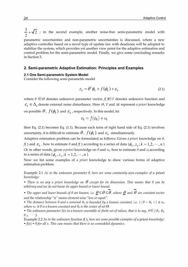
2.1 One Semi-parametric System ModelConsider the following semi-parametric model
k k k k f z ε φ φ θ τ ++= )( (2.1)
where θ Θ denotes unknown parameter vector, f (· ) F denotes unknown function and
k k Δ∈ε denote external noise disturbance. Here Θ, F and ∆k represent a priori knowledge
on possible θ , )( k f φ and k ε , respectively. In this model, let
then Eq. (2.1) becomes Eq. (1.1). Because each term of right hand side of Eq. (2.1) involves
uncertainty, it is difficult to estimate θ , )( k f φ and k ε simultaneously.
Adaptive estimation problem can be formulated as follows: Given a priori knowledge on θ,
f (· ) and k ε , how to estimate θ and f (· ) according to a series of data nk z k k ,,2,1;, L=φ
Or in other words, given a priori knowledge on θ and vk, how to estimate θ and vk according
to a series of data nk z k k ,,2,1;, L=φ .
Now we list some examples of a priori knowledge to show various forms of adaptiveestimation problem.
Example 2.1 As to the unknown parameter θ , here are some commonly-seen examples of a prioriknowledge:
• There is no any a priori knowledge on θ except for its dimension. This means that θ can bearbitrary and we do not know its upper bound or lower bound.
• The upper and lower bounds of θ are known, i.e. θ θ θ ≤≤ , where θ and θ are constant vector
and the relationship “≤” means element-wise “less or equal”.• The distance between θ and a nominal θ0 is bounded by a known constant, i.e. ||θ − θ0 || ≤ r θ ,where r θ ≥ 0 is a known constant and θ0 is the center of set Θ.• The unknown parameter lies in a known countable or finite set of values, that is to say, θ θ1 , θ2 ,θ 3 , · · · .Example 2.2 As to the unknown function f (· ) , here are some possible examples of a priori knowledge:• f (x) = 0 for all x. This case means that there is no unmodeled dynamics.
Adaptive Estimation and Control for Systems with Parametric and Nonparametric Uncertainties 25
• Function f is bounded by other known functions, that is to say, )()()( x f x f x f ≤≤ for any x.
• The distance between f and a nominal f 0 is bounded by a known constant, i.e. ||f − f 0|| ≤ r f ,where r f ≥ 0 is a known constant and f 0 can be regarded as the center of a ball F in a metric functionalspace with norm || · ||.• The unknown function lies in a known countable or finite set of functions, that is to say, f f 1 , f 2 , f 3 , · · · .
• Function f is Lipschitz, i.e. ||)()( 2121 x x L x f x f −≤− for some constant L > 0.
• Function f is monotone (increasing or decreasing) with respect to its arguments.• Function f is convex (or concave).• Function f is even (or odd).
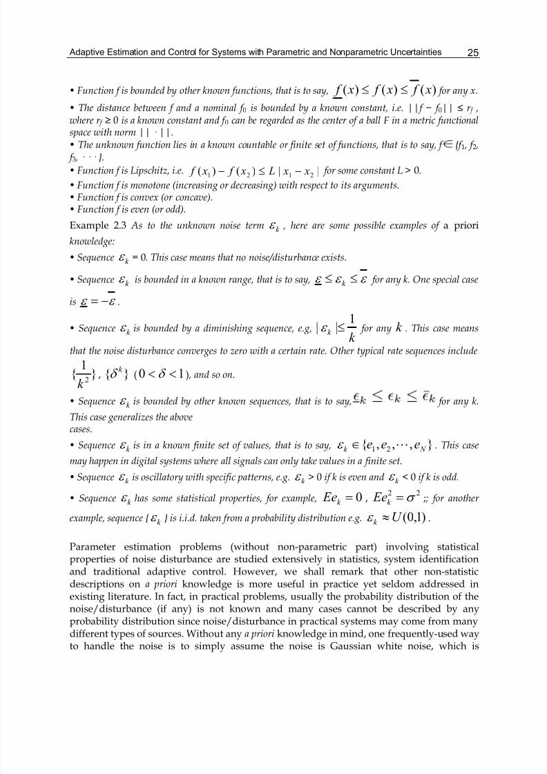
Example 2.3 As to the unknown noise term k ε , here are some possible examples of a priori
knowledge:
• Sequence k ε = 0. This case means that no noise/disturbance exists.
• Sequence k ε is bounded in a known range, that is to say, ε ε ε ≤≤ k for any k. One special case
is ε ε −= .
• Sequence k ε is bounded by a diminishing sequence, e.g,k
k
1|| ≤ε for any k . This case means
that the noise disturbance converges to zero with a certain rate. Other typical rate sequences include
1
2k
, k δ ( 10 << δ ) , and so on.
• Sequence k ε is bounded by other known sequences, that is to say, for any k.
This case generalizes the abovecases.
• Sequence k ε is in a known finite set of values, that is to say, ,,, 21 N k eee L∈ε . This case
may happen in digital systems where all signals can only take values in a finite set.
• Sequence k ε is oscillatory with specific patterns, e.g. k ε > 0 if k is even and k ε < 0 if k is odd.
• Sequence k ε has some statistical properties, for example, 0=k Ee ,22 σ =k Ee ; ; for another
example, sequence k ε is i.i.d. taken from a probability distribution e.g. )1,0(U k ≈ε .
Parameter estimation problems (without non-parametric part) involving statisticalproperties of noise disturbance are studied extensively in statistics, system identificationand traditional adaptive control. However, we shall remark that other non-statisticdescriptions on a priori knowledge is more useful in practice yet seldom addressed inexisting literature. In fact, in practical problems, usually the probability distribution of thenoise/disturbance (if any) is not known and many cases cannot be described by anyprobability distribution since noise/disturbance in practical systems may come from manydifferent types of sources. Without any a priori knowledge in mind, one frequently-used wayto handle the noise is to simply assume the noise is Gaussian white noise, which is
Adaptive Control26
reasonable in a certain sense. But in practice, from the point of view of engineering, we canusually conclude the noise/disturbance is bounded in a certain range. This chapter willfocus on uncertainties with non-statistical a priori knowledge. Without loss of generality, in
this section we often regard k k k f v ε φ += )( as a whole part, and correspondingly, a priori
knowledge on k v , (e.g. k k k vvv ≤≤ ), should be provided for the study.
2.2 An Example Problem
Now we take a simple example to show that it may not be appropriate to apply traditionalidentification algorithms blindly so as to get the estimate of unknown parameter.Consider the following system
k k k k k f z ε φ θφ ++= ),( (2.2)
where θ, f (· ) and k ε are unknown parameter, unknown function and unmeasurable noise,
respectively. For this model, suppose that we have the following a priori knowledge on thesystem:• No a priori knowledge on θ is known.
• At any step k, the term is of form . Here is anunknown sequence satisfying 0 ≤ ≤ 1.
• Noise k ε is diminishing with .
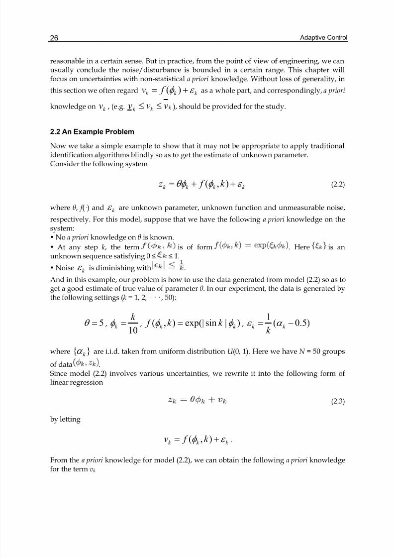
And in this example, our problem is how to use the data generated from model (2.2) so as toget a good estimate of true value of parameter θ. In our experiment, the data is generated bythe following settings (k = 1 , 2 , · · · , 50):
5=θ ,10
k k =φ , )|sinexp(|),( k k k k f φ φ = , )5.0(
1−= k k
k α ε
where k α are i.i.d. taken from uniform distribution U (0 , 1). Here we have N = 50 groups
of data .Since model (2.2) involves various uncertainties, we rewrite it into the following form oflinear regression
(2.3)
by letting
k k k k f v ε φ += ),( .
From the a priori knowledge for model (2.2), we can obtain the following a priori knowledgefor the term vk
Adaptive Estimation and Control for Systems with Parametric and Nonparametric Uncertainties 27
where
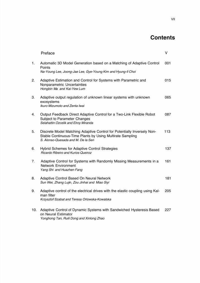
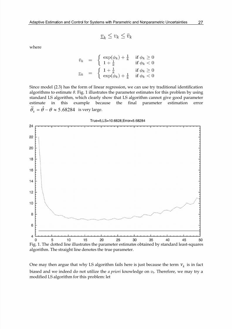
Since model (2.3) has the form of linear regression, we can use try traditional identificationalgorithms to estimate θ. Fig. 1 illustrates the parameter estimates for this problem by usingstandard LS algorithm, which clearly show that LS algorithm cannot give good parameterestimate in this example because the final parameter estimation error
68284.5ˆ~≈−= θ θ θ k
is very large.
Fig. 1. The dotted line illustrates the parameter estimates obtained by standard least-squaresalgorithm. The straight line denotes the true parameter.
One may then argue that why LS algorithm fails here is just because the term k v is in fact
biased and we indeed do not utilize the a priori knowledge on vk. Therefore, we may try amodified LS algorithm for this problem: let
Adaptive Control28
then we can conclude that k k k w y += φ θ τ and ],[ k k k d d w −∈ , where ],[ k k d d − is a
symmetric interval for every k. Then, intuitively, we can apply LS algorithm to data
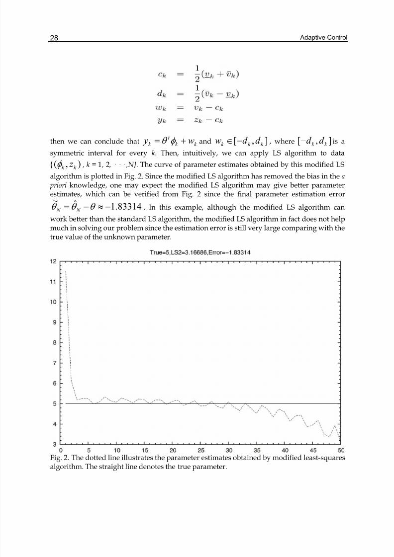
),( k k z φ , k = 1 , 2 , · · · ,N. The curve of parameter estimates obtained by this modified LS
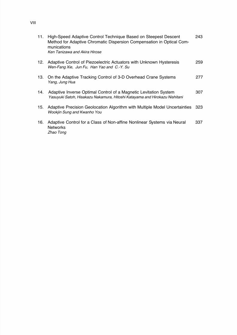
algorithm is plotted in Fig. 2. Since the modified LS algorithm has removed the bias in the a priori knowledge, one may expect the modified LS algorithm may give better parameterestimates, which can be verified from Fig. 2 since the final parameter estimation error
83314.1ˆ~−≈−= θ θ θ
N N . In this example, although the modified LS algorithm can
work better than the standard LS algorithm, the modified LS algorithm in fact does not helpmuch in solving our problem since the estimation error is still very large comparing with thetrue value of the unknown parameter.
Fig. 2. The dotted line illustrates the parameter estimates obtained by modified least-squaresalgorithm. The straight line denotes the true parameter.
Adaptive Estimation and Control for Systems with Parametric and Nonparametric Uncertainties 29
From this example, we do not aim to conclude that traditional identification algorithmsdeveloped in linear regression are not good, however, we want to emphasize the followingparticular point: Although traditional identification algorithms (such as LS algorithm) are very powerful and useful in practice, generally it is not wise to apply them blindly when the matchingconditions, which guarantee the convergence of those algorithms, cannot be verified or asserted a priori. This particular point is in fact one main reason why the so-called minimum-varianceself tuning regulator , developed in the area of adaptive control based on the LS algorithm,attracted several leading scholars to analyze its closed-loop stability throughout pastdecades from the early stage of adaptive control.To solve this example and many similar examples with a priori knowledge, we will proposenew ideas to estimate the parametric uncertainties and the non-parametric uncertainties.
2.3 Information-Concentration Estimator We have seen that there exist various forms of a priori knowledge on system model. With thea priori knowledge, how can we estimate the parametric part and the non-parametric part?Now we introduce the so-called information-concentration estimator. The basic idea of thisestimator is, the a priori knowledge at each time step can be regarded as some constraints ofthe unknown parameter or function, hence the growing data can provide more and moreinformation (constraints) on the true parameter or function, which enable us to reduce theuncertainties step by step. We explain this general idea by the simple model
(2.4)
with a priori knowledge thatk k
d V R ∈⊆Θ∈ υ θ , . Then, at k-th step (k ≥1), with the
current data k,k k z ,φ we can define the so-called information set I k at step k:
(2.5)
For convenience, let I 0 = Θ. Then we can define the so-called concentrated information set C k atstep k as follows
(2.6)
which can be recursively written as
(2.7)
with initial set C 0 = Θ. Eq. (2.7) with Eq. (2.5) is called information-concentration estimator
(short for IC estimator ) throughout this chapter, and any value in the set k C can be taken as
one possible estimate of unknown parameter θ at time step k . The IC estimator differs
from existing parameter identification in the sense that the IC estimator is in fact a set-

Adaptive Control30
valued estimator rather than a real-valued estimator. In practical applications, generally
k C is a domain ind
, and naturally we can take the center point of k C as k θ .
Remark 2.1 The definition of information set varies with system model. In general cases, it can be
extended to the set of possible instances of θ (and/or f ) which do not contradict with the data at
step k. We will see an example involving unknown f in next section.From the definition of the IC estimator, the following proposition can be obtained withoutdifficulty:
Proposition 2.1 Information-concentration estimator has the following properties:
(i) Monotonicity: L⊇⊇⊇ 210 C C C
(ii) Convergence: Sequence C k has a limit set k k C C
∞
=∞ ∩=
1 ;
(iii) If the system model and the a priori knowledge are correct, then must be a non-empty setwith property θ and any element of can match the data and the model;
(iv) If ∅=∞C , then the data , k k z φ cannot be generated by the system model used by the IC
estimator under the specified a priori knowledge.
Proposition 2.1 tells us the following particular points of the IC estimator: property (i)implies that the IC estimator will provide more and more exact estimation; property (ii)means that the there exists a limitation in the accuracy of estimation; property (iii) means
that true parameter lies in everyk C if the system model and a priori knowledge are correct;
and property (iv) means that the IC estimator provides also a method to validate the systemmodel and the a priori knowledge. Now we discuss the IC estimator for model (2.4) in moredetails. In the following discussions, we only consider a typical a priori knowledge on
k k k vvv ≤≤ are two known sequences of vectors (or scalars).
2.3.1 Scalar case: d = 1By Eq. (2.5), we have
Solving the inequality in I k, we obtain that

Adaptive Estimation and Control for Systems with Parametric and Nonparametric Uncertainties 31
and consequently, if 0≠k φ , then we have
where
Here sign(x) denotes the sign of x: sign(x) = 1 , 0 ,−1 for positive number, zero, and negativenumber, respectively. Then, by Eq. (2.7), we can explicitly obtain that
where and can be recursively obtained by
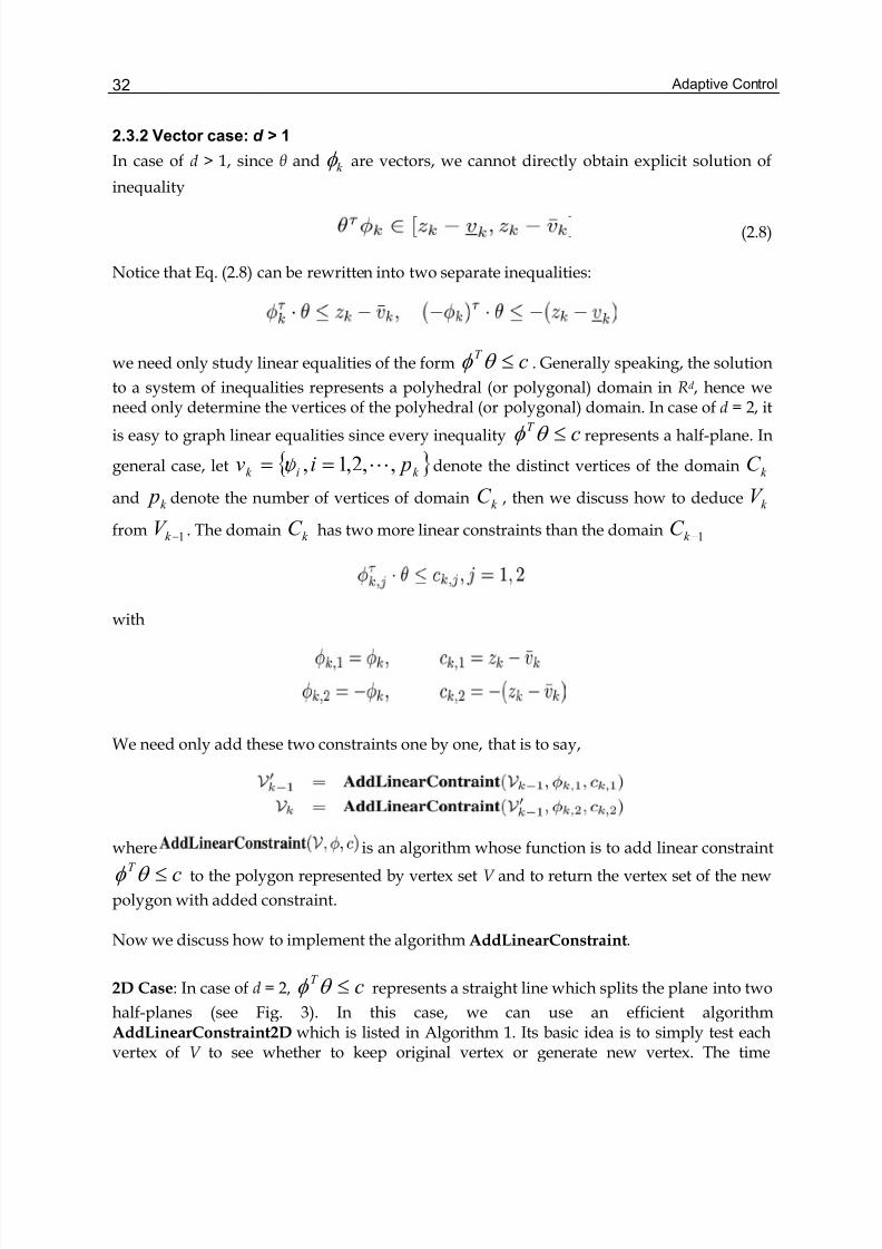
Fig. 3. The straight line may intersect the polygon V and split it into two sub-polygons, oneof which will become new polygon V'. The polygon V' can be efficiently calculated from thepolygon V .
Adaptive Control32
2.3.2 Vector case: d > 1
In case of d > 1, since θ and k φ are vectors, we cannot directly obtain explicit solution of
inequality
(2.8)
Notice that Eq. (2.8) can be rewritten into two separate inequalities:
we need only study linear equalities of the form cT ≤θ φ . Generally speaking, the solution
to a system of inequalities represents a polyhedral (or polygonal) domain in Rd, hence weneed only determine the vertices of the polyhedral (or polygonal) domain. In case of d = 2, it
is easy to graph linear equalities since every inequality cT ≤θ φ represents a half-plane. In
general case, let k ik piv ,,2,1, L=/= υ denote the distinct vertices of the domain k C
and k p denote the number of vertices of domain k C , then we discuss how to deduce k V
from 1−k V . The domain k C has two more linear constraints than the domain 1−k C
with
We need only add these two constraints one by one, that is to say,
where is an algorithm whose function is to add linear constraint
cT ≤θ φ to the polygon represented by vertex set V and to return the vertex set of the new
polygon with added constraint.
Now we discuss how to implement the algorithm AddLinearConstraint.
2D Case: In case of d = 2, cT ≤θ φ represents a straight line which splits the plane into two
half-planes (see Fig. 3). In this case, we can use an efficient algorithmAddLinearConstraint2D which is listed in Algorithm 1. Its basic idea is to simply test eachvertex of V to see whether to keep original vertex or generate new vertex. The time

Adaptive Estimation and Control for Systems with Parametric and Nonparametric Uncertainties 33
complexity of Algorithm 1 is O(s), where s is the number of vertices of domain V . Note that
it is possible that V' = Ø if the straight line L : cT ≤θ φ does not intersect with the polygon
V and any vertex i P of polygon V does not satisfy c P iT
>φ . And the vertex number of
polygon 'V can in fact vary within the range from 0 to s according to the geometric
relationship between the straight line L and the polygon V .
High-dimensional Case: In case of d > 2, cT ≤θ φ represents a hyperplane which splits
the whole space into two half-hyperplanes.Unlike in case of d = 2, the vertices in this case generally cannot be arranged in a certainnatural order (such as clock-wise order). In this case, we can use an algorithmAddLinearConstraintND which is listed in Algorithm 2. The idea of this algorithm is toclassify the vertices of V first according to their relationship with the hyperplane determined
by hyperplane cT ≤θ φ .
Algorithm 2 AddLinearConstraintND(V, ", c): Add linear constraint cT ≤θ φ (" % Rd) to a
polyhedron V
2.3.3 Implementation issuesIn the IC estimator, the key problem is to calculate the information set I k or the concentratedinformation set C k at every step. From the discussions above, we can see that it is easy tosolve this basic problem in case of d = 1. However, in case of d > 1, generally the vertex

Adaptive Control34
number of domain k C may grow as ∞→k . Therefore, it may be impractical to
implement the IC estimator in case of d > 1 since it may require growing memory as
∞→k To overcome this problem, noticing the fact that the domain C k will shrink
gradually as ∞→k in order to get a feasible IC estimate of the unknown parameter
vector, generally we need not use too many vertices to represent the exact concentratedinformation set C k. That is to say, in practical implementation of IC estimator in high-dimensional case, we can use a domain Ĉk with only a small number (say up to M ) ofvertices to approximate the exact concentrated information set C k. With such an idea ofapproximate IC estimator , the issue of computational complexity will not hinder theapplications of IC estimator.
We consider two typical cases of approximate IC estimator . One typical case is that
for any k, and the other case is that for any k. Let k k C C ˆˆ
1
∞
=∞
∩= , then in the
former case (called loose IC estimator , see Fig. 4), we must have
which means that we will never mistakenly exclude the true parameter from theconcentrated approximate information sets; while in the latter case (called tight IC estimator ,see Fig. 5), we must have
which means that the true parameter may be outside of ∞C ˆ however any value in ∞
C ˆ can
be served as good estimate of true parameter.
Fig. 4. Idea of loose IC estimator: The polygon P1P2P3P4P5 can be approximated by a triangleQ1P4Q2. Here M = 3.
Adaptive Estimation and Control for Systems with Parametric and Nonparametric Uncertainties 35
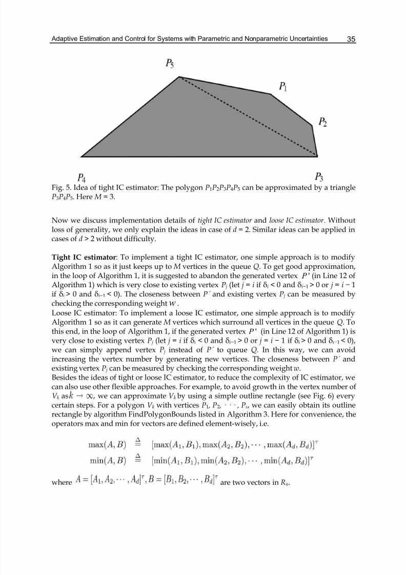
Fig. 5. Idea of tight IC estimator: The polygon P1P2P3P4P5 can be approximated by a triangleP3P4P5. Here M = 3.
Now we discuss implementation details of tight IC estimator and loose IC estimator . Withoutloss of generality, we only explain the ideas in case of d = 2. Similar ideas can be applied incases of d > 2 without difficulty.
Tight IC estimator: To implement a tight IC estimator, one simple approach is to modifyAlgorithm 1 so as it just keeps up to M vertices in the queue Q. To get good approximation,in the loop of Algorithm 1, it is suggested to abandon the generated vertex ' P (in Line 12 ofAlgorithm 1) which is very close to existing vertex P j (let j = i if δi < 0 and δi−1 > 0 or j = i − 1if δi > 0 and δi−1 < 0). The closeness between P´ and existing vertex P j can be measured bychecking the corresponding weightw .
Loose IC estimator: To implement a loose IC estimator, one simple approach is to modifyAlgorithm 1 so as it can generate M vertices which surround all vertices in the queue Q. Tothis end, in the loop of Algorithm 1, if the generated vertex ' P (in Line 12 of Algorithm 1) isvery close to existing vertex P j (let j = i if δi < 0 and δi−1 > 0 or j = i − 1 if δi > 0 and δi−1 < 0),we can simply append vertex P j instead of P´ to queue Q. In this way, we can avoidincreasing the vertex number by generating new vertices. The closeness between P´ andexisting vertex P j can be measured by checking the corresponding weight w.Besides the ideas of tight or loose IC estimator, to reduce the complexity of IC estimator, wecan also use other flexible approaches. For example, to avoid growth in the vertex number ofV k as , we can approximate V k by using a simple outline rectangle (see Fig. 6) everycertain steps. For a polygon V k with vertices P1 , P2 , · · · , Ps, we can easily obtain its outlinerectangle by algorithm FindPolygonBounds listed in Algorithm 3. Here for convenience, theoperators max and min for vectors are defined element-wisely, i.e.
where are two vectors in Rn.

Adaptive Control36
Fig. 6. Idea of outline rectangle: The polygon 54321 P P P P P can be approximated by an
outline rectangle. In this case, 11, B B denote the lower bound and upper bound in the x-
axis (1st component of each vertex), and 22 , B B denote the lower bound and upper bound
in the y-axis (2nd component of each vertex)
2.4 IC Estimator vs. LS Estimator
2.4.1 Illustration of IC Estimator
Now we go back to the example problem discussed before. For this example, k φ and zk are
scalars, hence we need only apply the IC estimator introduced in Section 2.3.1. Since IC
estimator yields concentrated information set k C at every step, we can take any value in
Adaptive Estimation and Control for Systems with Parametric and Nonparametric Uncertainties 37
k C as parameter estimate of true parameter. In this example, k C is an interval at every
step step. For comparison with other parameter estimation methods, we simply take
)(2
1ˆk k k bb +=θ , i.e. the center of interval k C , as the parameter estimate at step k.
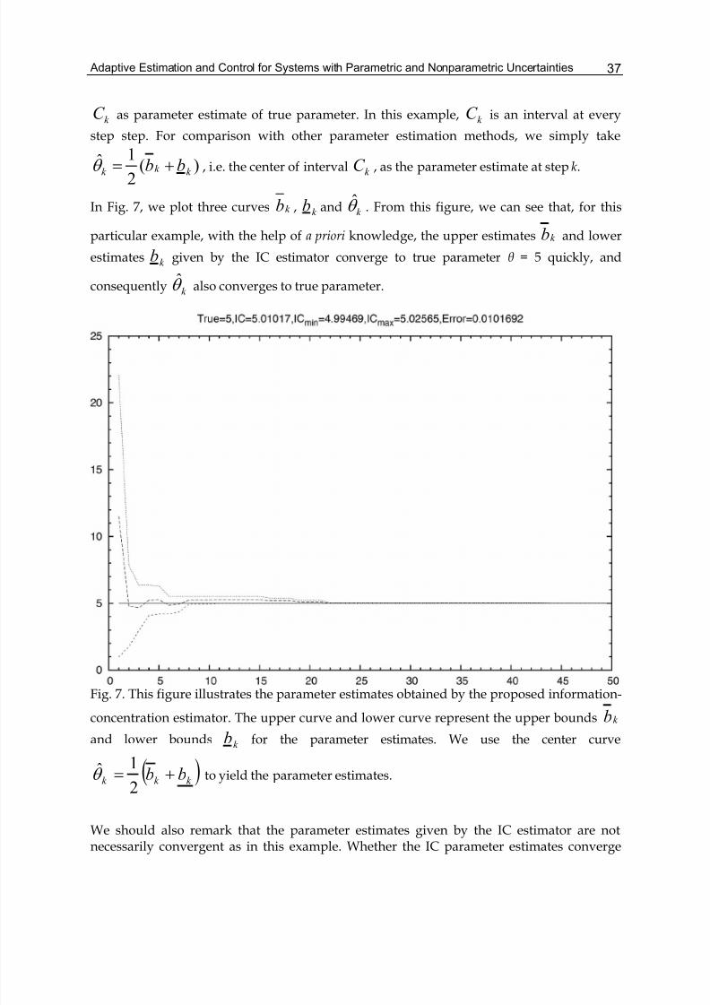
In Fig. 7, we plot three curves k b , k b and k θ . From this figure, we can see that, for this
particular example, with the help of a priori knowledge, the upper estimates k b and lower
estimates k b given by the IC estimator converge to true parameter θ = 5 quickly, and
consequently k θ also converges to true parameter.
Fig. 7. This figure illustrates the parameter estimates obtained by the proposed information-
concentration estimator. The upper curve and lower curve represent the upper bounds k b
and lower bounds k b for the parameter estimates. We use the center curve
( )k k k bb +=2
1θ to yield the parameter estimates.
We should also remark that the parameter estimates given by the IC estimator are notnecessarily convergent as in this example. Whether the IC parameter estimates converge

Adaptive Control38
largely depend on the accuracy of a priori knowledge and the richness of the practical data.Note that the IC estimator generally does not require classical richness concepts (like persistent excitation) which are useful in the analysis of traditional recursive identificationalgorithms.
2.4.2 Advantages of IC Estimator
We have seen practical effects of IC estimator for the simple example given above. Why canit perform better than the LS estimator? Roughly speaking, comparing with traditionalidentification algorithm like LS algorithm, the proposed IC estimator has the followingadvantages:
1. It can make full use of a priori information and posterior information. And in the idealcase, no information is wasted in the iteration process of the IC estimator. This property isnot seen in traditional identification algorithms since only partial information and certainstochastic a priori knowledge can be utilized in those algorithms.2. It does not give single parameter estimate at every step; instead, it gives a (finite orinfinite) set of parameter estimates at every step. This property is also unique sincetraditional identification algorithms always give parameter estimates directly.3. It can gradually find out all (or most) possible values of true parameters; and thisproperty can even help people to check the consistence between the practical data and thesystem model with a priori knowledge. This property distinguishes traditional identificationalgorithms in sense that traditional identification algorithms generally have no mechanismto validate the correctness of the system model.4. The a priori knowledge can vary from case to case, not necessarily described in thelanguage of probability theory or statistics. This property enables the IC estimator to handlevarious kinds of non-statistic a priori knowledge, which cannot be dealt with by traditionalidentification algorithms.5. It has great flexibilities in its implementation, and its design is largely determined by thecharacteristics of a priori knowledge. The IC estimator has only one basic principle—informationconcentration! Any practical implementation approach using such a principle can beregarded as an IC estimator. We have discussed some implementation details for a certaintype of IC estimator in last subsection, which have shown by examples how to design the ICestimator according the known a priori knowledge and how to reduce computationalcomplexity in practical implementation.6. Its accuracy will never degrade as time goes by. Generally speaking, the more stepscalculated, the more data involved, and the more accurate the estimates are. Generallyspeaking, traditional identification algorithms can only have similar property (called strongconsistency) under certain matching conditions.7. The IC estimator can not only provide reasonably good parameter estimates but also tellpeople how accurate these estimates are. In our previous example, when we use
( )k k k bb +=
2
1θ as the parameter estimate, we know also that the absolute parameter
estimation error θ θ θ −= ˆ~ will not exceed ( )k k bb +2
1. In some sense, such a property
may be conceptually similar to the so-called confidence level in statistics.
Adaptive Estimation and Control for Systems with Parametric and Nonparametric Uncertainties 39
2.4.3 Disadvantages of IC Estimator Although the IC estimator has many advantages over traditional identification algorithms, itmay have the following disadvantages:
1. The proposed IC estimator is relatively difficult to incorporate stochastic a prioriknowledge on noise term, especially unbounded random noise. In fact, in such caseswithout non-parametric uncertainties, traditional identification algorithms like LS algorithmmay be more suitable and efficient to estimate the unknown parameter.2. The efficiency of IC estimator largely depends on its implementation via thecharacteristics of the a priori knowledge. Generally speaking, the IC estimator may involve alittle more computation operations than recursive identification algorithms like LSalgorithm. We shall remark also that this point is not always true since the numericaloperations involved in the IC estimator are relatively simple (see algorithms listed before),while many traditional identification algorithms may involve costly numerical operationslike matrix product, matrix inversion, etc.3. Although the IC estimator has simple and elegant properties such as monotonicity andconvergence, due to its nature of set-valued estimator , no explicit and recursive expressions canbe given directly for the IC parameter estimates, which may bring mathematical difficultiesin the applications of the IC estimator. However, generally speaking, we also know that closed-loop analysis for adaptive control using traditional identification algorithms is noteasy, too.
Summarizing the above, we can conclude that the IC estimator provides a new approach orprinciple to estimate parametric and even non-parametric uncertainties, and we have shownthat it is possible to design efficient IC estimator according to characteristics of a prioriknowledge.
3. Semi-parametric Adaptive Control: Example 1
In this section, we will give a first example of semi-parametric adaptive control, whosedesign is essentially based on the IC estimator introduced in last section.
3.1 Problem Formulation
Consider the following system
(3.1)
where yt, ut and wt are the output, input and noise, respectively; )()( L F f ∈⋅ is an
unknown function (the set F (L) will be defined later) and θ is an unknown parameter. To
make further study, the following assumptions are used throughout this section:
Assumption 3.1 The unknown function R R f →: belongs to the following uncertainty set
(3.2)
Adaptive Control40
where c is an arbitrary non-negative constant.
Assumption 3.2 The noise sequence t w is bounded, i.e.
where w is an arbitrary positive constant.
Assumption 3.3 The tracking signal *
t y is bounded, i.e.
(3.3)where S is a positive constant.
Assumption 3.4 In the parametric part t θφ , we have no any a priori information of the unknown
parameter θ , but )( t t y g =φ is measurable and satisfies
(3.4)
for any 21 x x ≠ , where M' ≤ M are two positive constants and 1≥b is a constant.
Remark 3.1 Assumption 3.4 implies that function g(· ) has linear growth rate when b = 1. Especiallywhen g(x) = x, we can take M = M' = 1. Condition (3.4) need only hold for sufficiently large x1 andx2 , however we require it holds for all x1 ≠ x2 to simplify the proof. We shall also remark that Sokolov[Sok03] has ever studied the adaptive estimation and control problem for a special case of model (3.1),
where t φ is simply taken as t ay .
Remark 3.2 Assumption 3.4 excludes the case where g(· ) is a bounded function, which can be
handled easily by previous research. In fact, in that case 11'++
+= t t t ww θφ must be bounded,
hence by the result of [XG00], system (3.1) is stabilizable if and only if 22
3+< L .
3.2 Adaptive Controller DesignIn the sequel, we shall construct a unified adaptive controller for both cases of b =1 and b >1.For convenience, we introduce some notations which are used in later parts. Let I = [a, b] be
an interval, then )(2
1)( ba I m +=Δ
(a+ b) denotes the center point of interval I , and
( ) ab I r −=Δ
2
1denotes the radius of interval I . And correspondingly, we let
( ) [ ]δ δ δ +−= x x x I ,, denote a closed interval centered at R x∈ with radius δ ≥ 0.
Estimate of Parametric Part: At time t, we can use the following information: y0 , y1 , · · · , yt,
u0 , u1 , · · · , ut−1 and t φ φ φ ,,, 21 L . Define
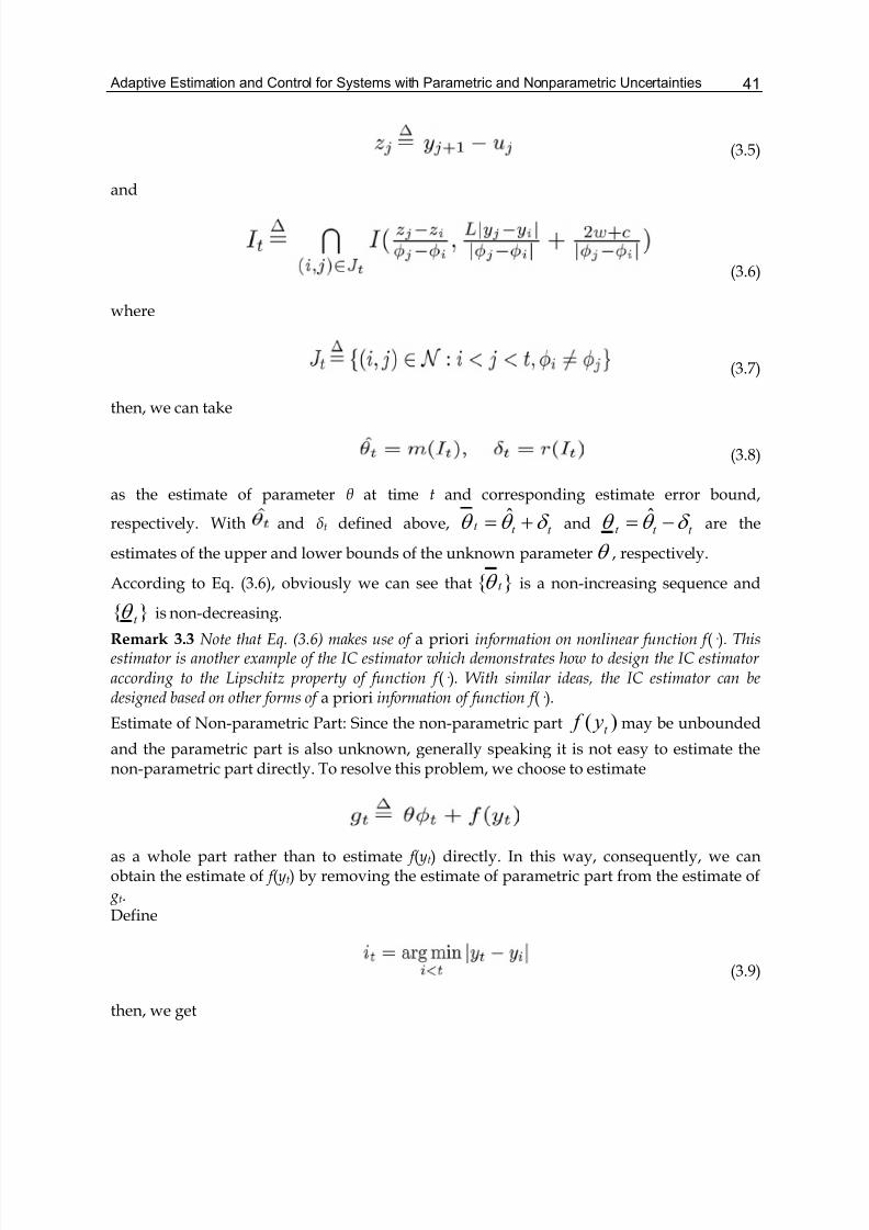
Adaptive Estimation and Control for Systems with Parametric and Nonparametric Uncertainties 41
(3.5)
and
(3.6)
where
(3.7)
then, we can take
(3.8)
as the estimate of parameter θ at time t and corresponding estimate error bound,
respectively. With and δ t defined above, t t t δ θ θ += ˆ and t t t δ θ θ −= ˆ are the
estimates of the upper and lower bounds of the unknown parameterθ , respectively.
According to Eq. (3.6), obviously we can see that t θ is a non-increasing sequence and
t θ is non-decreasing.
Remark 3.3 Note that Eq. (3.6) makes use of a priori information on nonlinear function f (· ). Thisestimator is another example of the IC estimator which demonstrates how to design the IC estimator according to the Lipschitz property of function f (· ). With similar ideas, the IC estimator can bedesigned based on other forms of a priori information of function f (· ).
Estimate of Non-parametric Part: Since the non-parametric part )( t y f may be unbounded
and the parametric part is also unknown, generally speaking it is not easy to estimate thenon-parametric part directly. To resolve this problem, we choose to estimate
as a whole part rather than to estimate f (yt) directly. In this way, consequently, we canobtain the estimate of f (yt) by removing the estimate of parametric part from the estimate of gt.Define
(3.9)
then, we get
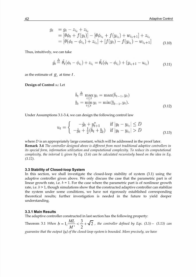
Adaptive Control42
(3.10)
Thus, intuitively, we can take
(3.11)
as the estimate of t g at time t .
Design of Control ut: Let
(3.12)
Under Assumptions 3.1-3.4, we can design the following control law
(3.13)
where D is an appropriately large constant, which will be addressed in the proof later.Remark 3.4 The controller designed above is different from most traditional adaptive controllers inits special form, information utilization and computational complexity. To reduce its computationalcomplexity, the interval I t given by Eq. (3.6) can be calculated recursively based on the idea in Eq.(3.12).
3.3 Stability of Closed-loop SystemIn this section, we shall investigate the closed-loop stability of system (3.1) using theadaptive controller given above. We only discuss the case that the parametric part is oflinear growth rate, i.e. b = 1. For the case where the parametric part is of nonlinear growthrate, i.e. b > 1, though simulations show that the constructed adaptive controller can stabilizethe system under some conditions, we have not rigorously established correspondingtheoretical results; further investigation is needed in the future to yield deeperunderstanding.
3.3.1 Main ResultsThe adaptive controller constructed in last section has the following property:
Theorem 3.1 When 22
3
',1 +<=
M
MLb , the controller defined by Eqs. (3.5)— (3.13) can
guarantee that the output yt of the closed-loop system is bounded. More precisely, we have
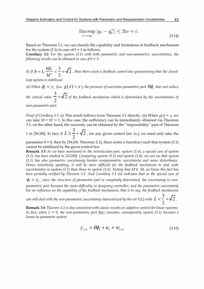
Adaptive Estimation and Control for Systems with Parametric and Nonparametric Uncertainties 43
(3.14)
Based on Theorem 3.1, we can classify the capability and limitations of feedback mechanismfor the system (3.1) in case of b = 1 as follows:Corollary 3.1 For the system (3.1) with both parametric and non-parametric uncertainties, the following results can be obtained in case of b = 1:
(i) If 22
3
',1 +<=
M
MLb , then there exists a feedback control law guaranteeing that the closed-
loop system is stabilized.
(ii) When t t y=φ (i.e. x x g =)( ) , the presence of uncertain parametric part t θφ does not reduce
the critical value 22
3+ of the feedback mechanism which is determined by the uncertainties of
non-parametric part.
Proof of Corollary 3.1: (i) This result follows from Theorem 3.1 directly. (ii) When g(x) = x, wecan take M = M´ = 1. In this case, the sufficiency can be immediately obtained via Theorem3.1; on the other hand, the necessity can be obtained by the “impossibility” part of Theorem
1 in [XG00]. In fact, if 22
3+≥ L , for any given control law ut , we need only take the
parameter θ = 0, then by [XG00, Theorem 2.1], there exists a function f such that system (3.1)cannot be stabilized by the given control law.Remark 3.5 As we have mentioned in the introduction part, system (1.6), a special case of system(3.1), has been studied in [XG00]. Comparing system (3.1) and system (1.6), we can see that system(3.1) has also parametric uncertainty besides nonparametric uncertainty and noise disturbance.Hence intuitively speaking, it will be more difficult for the feedback mechanism to deal withuncertainties in system (3.1) than those in system (1.6). Noting that M'≤ M, we know this fact hasbeen partially verified by Theorem 3.1. And Corollary 3.1 (ii) indicates that in the special case of
t t y=φ , since the structure of parametric part is completely determined, the uncertainty in non-
parametric part becomes the main difficulty in designing controller, and the parametric uncertaintyhas no influence on the capability of the feedback mechanism, that is to say, the feedback mechanism
can still deal with the non-parametric uncertainty characterized by the set F (L) with 22
3+< L .
Remark 3.6 Theorem 3.1 is also consistent with classic results on adaptive control for linear systems.In fact, when L = 0 , the non-parametric part f (yt) vanishes, consequently system (3.1) becomes alinear-in-parameter system
11 ++ ++= t t t t wu y θφ (3.15)
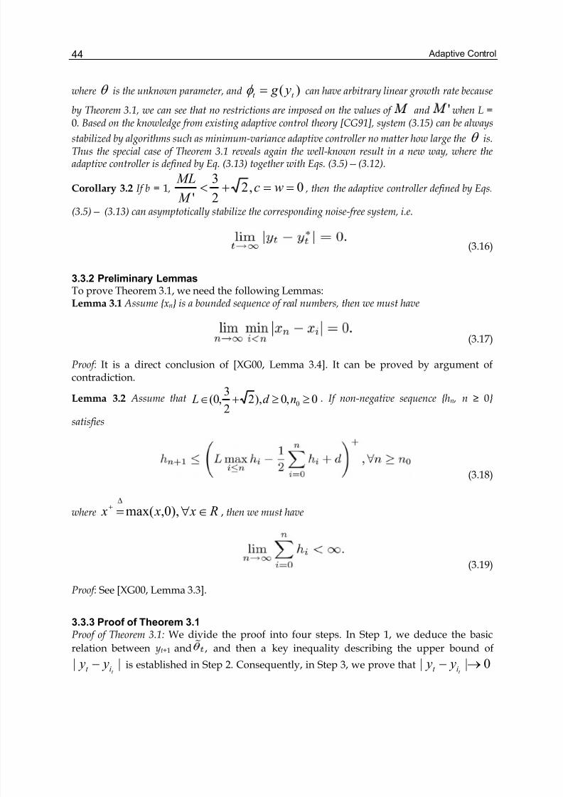
Adaptive Control44
where θ is the unknown parameter, and )( t t y g =φ can have arbitrary linear growth rate because
by Theorem 3.1, we can see that no restrictions are imposed on the values of and ' when L =0. Based on the knowledge from existing adaptive control theory [CG91], system (3.15) can be always
stabilized by algorithms such as minimum-variance adaptive controller no matter how large the θ is.Thus the special case of Theorem 3.1 reveals again the well-known result in a new way, where theadaptive controller is defined by Eq. (3.13) together with Eqs. (3.5)—(3.12).
Corollary 3.2 If b = 1 , 0,22
3
'==+< wc
M
ML , then the adaptive controller defined by Eqs.
(3.5)— (3.13) can asymptotically stabilize the corresponding noise-free system, i.e.
(3.16)
3.3.2 Preliminary LemmasTo prove Theorem 3.1, we need the following Lemmas:Lemma 3.1 Assume xn is a bounded sequence of real numbers, then we must have
(3.17)
Proof: It is a direct conclusion of [XG00, Lemma 3.4]. It can be proved by argument ofcontradiction.
Lemma 3.2 Assume that 0,0),22
3,0( 0 ≥≥+∈ nd L . If non-negative sequence hn , n ≥ 0
satisfies
(3.18)
where R x x x ∈∀=Δ
+ ),0,max( , then we must have
(3.19)
Proof: See [XG00, Lemma 3.3].
3.3.3 Proof of Theorem 3.1
Proof of Theorem 3.1: We divide the proof into four steps. In Step 1, we deduce the basic
relation between yt+1 and , and then a key inequality describing the upper bound of
||t it y y − is established in Step 2. Consequently, in Step 3, we prove that 0|| →−
t it y y
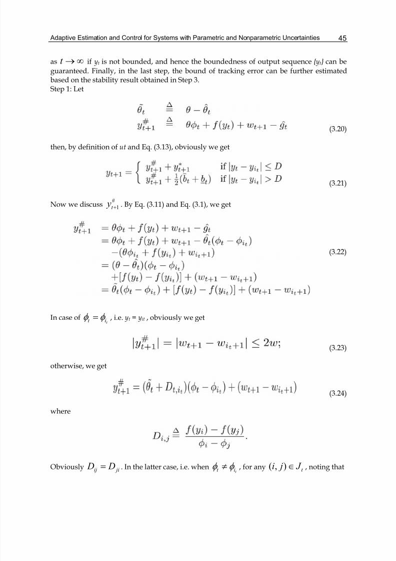
Adaptive Estimation and Control for Systems with Parametric and Nonparametric Uncertainties 45
as ∞→t if yt is not bounded, and hence the boundedness of output sequence yt can be
guaranteed. Finally, in the last step, the bound of tracking error can be further estimatedbased on the stability result obtained in Step 3.Step 1: Let
(3.20)
then, by definition of ut and Eq. (3.13), obviously we get
(3.21)
Now we discuss#
1+t y . By Eq. (3.11) and Eq. (3.1), we get
(3.22)
In case oft it φ φ = , i.e. yt = yit , obviously we get
(3.23)
otherwise, we get
(3.24)
where
Obviously jiij D D = . In the latter case, i.e. whent it φ φ ≠ , for any t J ji ∈),( , noting that
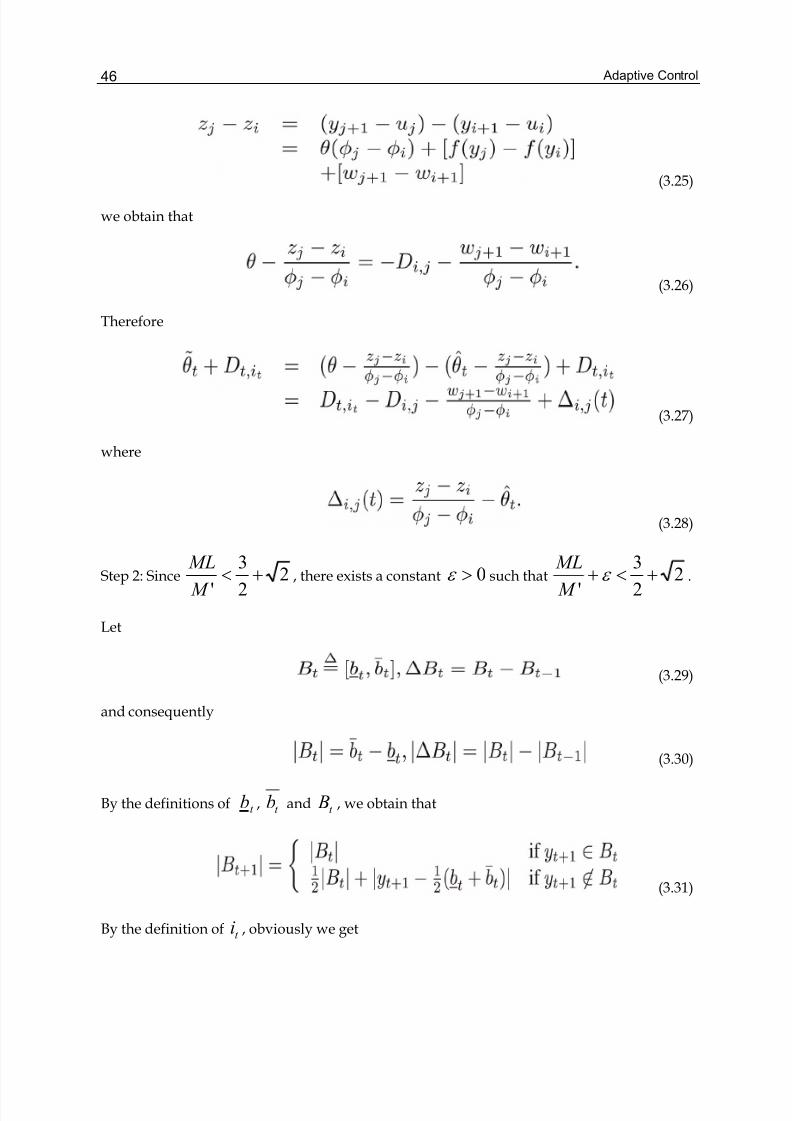
Adaptive Control46
(3.25)
we obtain that
(3.26)
Therefore
(3.27)
where
(3.28)
Step 2: Since 22
3
'+<
M
ML, there exists a constant 0>ε such that 2
2
3
'+<+ ε
M
ML.
Let
(3.29)
and consequently
(3.30)
By the definitions of t b , t b and t B , we obtain that
(3.31)
By the definition of t i , obviously we get
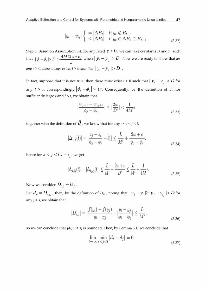
Adaptive Estimation and Control for Systems with Parametric and Nonparametric Uncertainties 47
(3.32)
Step 3: Based on Assumption 3.4, for any fixed 0>ε , we can take constants D andD´ such
thatε
φ φ )2(4
|| ' cw M D ji
+>>− when D y y
t it >− || . Now we are ready to show that for
any s > 0 , there always exists t > s such that D y yt it >− || .
In fact, suppose that it is not true, then there must exist s > 0 such that D y yt it >− || for
any t > s, correspondingly it t φ φ − > D´ . Consequently, by the definition of D, for
sufficiently large t and j < t, we obtain that
(3.33)
together with the definition of t θ , we know that for any s < i < j < t,
(3.34)
hence for jiit j s =<< , , we get
(3.35)
Now we consider jt i jit D D ,, − .
Letninn Dd ,= , then, by the definition of Di,j , noting that D y y y y
ji ji j >−≥− |||| for
any j > s, we obtain that
(3.36)
so we can conclude that dn , n > s is bounded. Then, by Lemma 3.1, we conclude that
(3.37)
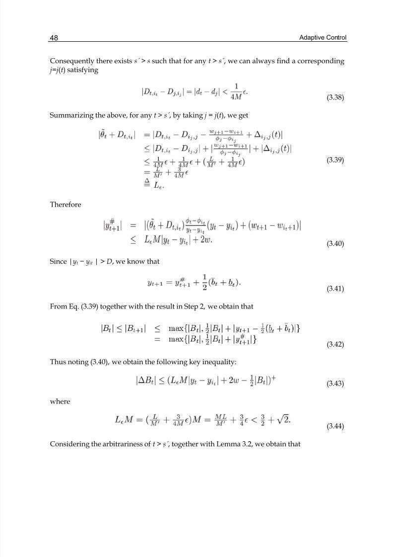
Adaptive Control48
Consequently there exists s´ > s such that for any t > s´ , we can always find a corresponding j= j(t) satisfying
(3.38)
Summarizing the above, for any t > s´ , by taking j = j(t), we get
(3.39)
Therefore
(3.40)
Since |yt − yit | > D, we know that
(3.41)
From Eq. (3.39) together with the result in Step 2, we obtain that
(3.42)
Thus noting (3.40), we obtain the following key inequality:
(3.43)
where
(3.44)
Considering the arbitrariness of t > s´ , together with Lemma 3.2, we obtain that
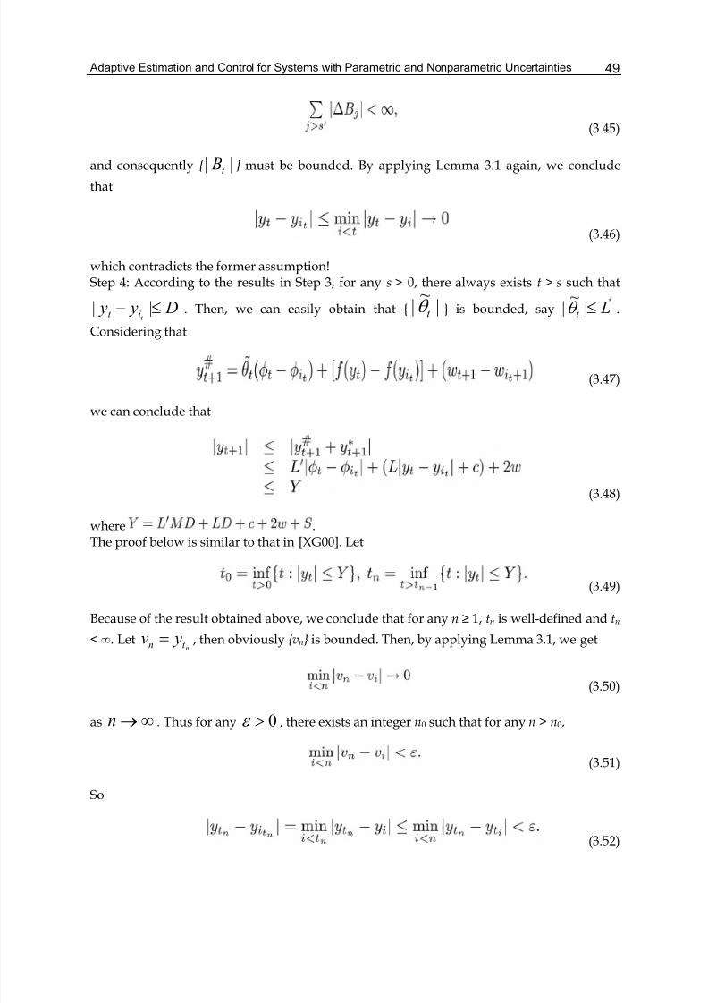
Adaptive Estimation and Control for Systems with Parametric and Nonparametric Uncertainties 49
(3.45)
and consequently || t B must be bounded. By applying Lemma 3.1 again, we conclude
that
(3.46)
which contradicts the former assumption!Step 4: According to the results in Step 3, for any s > 0, there always exists t > s such that
D y yt it ≤− || . Then, we can easily obtain that |
~| t θ is bounded, say
'|~
| Lt ≤θ .
Considering that
(3.47)
we can conclude that
(3.48)
where .The proof below is similar to that in [XG00]. Let
(3.49)
Because of the result obtained above, we conclude that for any n ≥ 1, tn is well-defined and tn
< ∞. Letnt n yv = , then obviously vn is bounded. Then, by applying Lemma 3.1, we get
(3.50)
as ∞→n . Thus for any 0>ε , there exists an integer n0 such that for any n > n0,
(3.51)
So
(3.52)
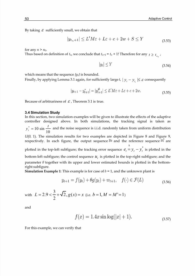
Adaptive Control50
By taking ε sufficiently small, we obtain that
(3.53)
for any n > n0.Thus based on definition of tn, we conclude that tn+1 = tn + 1! Therefore for any
0nt t ≥ ,
(3.54)
which means that the sequence yt is bounded.
Finally, by applying Lemma 3.1 again, for sufficiently large t, ε ≤− ||t it y y consequently
(3.55)
Because of arbitrariness of ε , Theorem 3.1 is true.
3.4 Simulation StudyIn this section, two simulation examples will be given to illustrate the effects of the adaptivecontroller designed above. In both simulations, the tracking signal is taken as
10sin10* t
yt = and the noise sequence is i.i.d. randomly taken from uniform distribution
U (0 , 1). The simulation results for two examples are depicted in Figure 8 and Figure 9,
respectively. In each figure, the output sequence and the reference sequence are
plotted in the top-left subfigure; the tracking error sequence*
t t t y ye −=Δ
is plotted in the
bottom-left subfigure; the control sequence t u is plotted in the top-right subfigure; and the
parameter θ together with its upper and lower estimated bounds is plotted in the bottom-right subfigure.Simulation Example 1: This example is for case of b = 1, and the unknown plant is
(3.56)
with x x g L =+<= )(,22
39.2 (i.e. 1',1 === M M b )
and
(3.57)
For this example, we can verify that
Adaptive Estimation and Control for Systems with Parametric and Nonparametric Uncertainties 51
(3.58)
consequently |||)()(| y x L y f x f −<− , i.e. )()( L F f ∈⋅ ..
Simulation Example 2: This example is for case of b > 1, and the unknown plant is
(3.59)
with 9.2= L ,2)( x x g = (i.e. 2=b , 1'
== ), and
(3.60)
For this example, we can verify that 2|||)()(| +−<− y x L y f x f , i.e. )()( L F f ∈⋅ .
From the simulation results, we can see that in both examples, the adaptive controller cantrack the reference signal successfully. The simulation study verified our theoretical resultand indicate that under some conditions, the adaptive control law constructed in this papercan deal with both parametric and non-parametric uncertainties, even in some cases whenthe parametric part is of nonlinear growth rate. In case of b = 1, the stabilizability criteriahave been completely characterized by a simple algebraic condition; however, in case of b >1, it is very difficult to give complete theoretical characterization. Note that usually moreaccurate estimate of parameter can be obtained in case of b > 1 than in case of b = 1,however, worse transient performance may be encountered.
Fig. 8. Simulation example 1: ( g(x) = x, b = 1 ,M = M´ = 1)
Adaptive Control52
Fig. 9. Simulation example 2: ( g(x) = x2 , b = 2 ,M = M´ = 1)
4. Semi-parametric Adaptive Control: Example 2
In this section, we shall give another example of adaptive estimation and control for a semi-parametric model. Although the system considered in this section is similar to the modelconsidered in last section, there are several particular points in this example:
• The controller gain in this model is also unknown with a priori knowledge on its sign andits lower bound.
• The system is noise-free, and correspondingly the asymptotic tracking is rigorouslyestablished in this example.
• The algorithm in this example has a form of gradient algorithm, however, it partiallymakes use of a priori knowledge on the non-parametric part.
• Due to the limitation of this algorithm and technical difficulties, unlike the algorithm inlast section, we can only establish stability of the closed-loop system under condition
5.00 << L for the parametric part, which is much stronger than the condition
22
30 +<≤ L
.
This example is given here only for the purpose of demonstrating that there exist otherpossible ways to make use of a priori knowledge on the parametric uncertainties and non-parametric uncertainties. By comparing the examples in this section and last section, thereaders may get a deeper understanding to adaptive estimation and control problems forsemi-parametric models.
Adaptive Estimation and Control for Systems with Parametric and Nonparametric Uncertainties 53
4.1 Problem Formulation
We consider the following system model
(4.1)
where1 R yk ∈ and
1 Ruk ∈ are output and control signals, respectively. Here1 R∈θ is
the unknown parameter,1 Rb∈ is the unknown controller gain, )(⋅Φ is a known function,
and f (· ) is the unknown function. We have the following a priori knowledge on the realsystem:
Assumption 4.1 The nonparametric uncertain function f (· ) is Lipschitz, i.e.,
R x x x x L x f x f ∈∀−≤− 212121 ,||,||||)()(|| , where L < 0.5. The known function )(⋅Φ is also a
Lipschitz function with Lipschitz constant L.
Assumption 4.2 The sign of unknown controller gain b is known. Without loss of generality, we
assume that 0>≥ bb where b is a known constant.
Assumption 4.3 The reference signal*
k y is a known bounded deterministic signal.
The control objective is to design the control law k u such that the output signal yk
asymptotically tracks a bounded reference trajectory*
k y and all the closed-loop signals are
guaranteed to be bounded.
4.2 Adaptive Control DesignTo design the adaptive controller, the following notations will be used throughtout thissection:
(4.2)
Obviously, at time step k, with the history information y j , j ≤ k and the a priori knowledge,
the index k l and the tracking error k e are available. Later we will see important roles of
k l and k e in the controller design.
Estimation of parametric part: The estimates of the parameter θ and the controller gain b at
time step k are denoted by and , respectively. We design the following adaptiveupdate law to update the parameter estimates recursively:
Adaptive Control54
where 10 << γ and the coefficient k a is defined by a time-varying deadzone:
(4.4)
Estimation of non-parametric part: As in last section, we do not estimate the non-parametric part directly. Instead, we try to estimate the parametric part and non-parametric part as a whole part
(4.5)
Noticing of the system model (4.1), we know that
(4.6)
consequently, from Eqs. (4.5) and (4.6), it is easy to derive
(4.7)
Since function f (· ) is unknown and parameters θ and b are unknown, we simply estimate#
k y by the following eqution
(4.8)
where and are regarded as true parameters, and the unknown term
)()(k l k y f y f − in Eq. (4.7) is simply dropped off.
Adaptive Estimation and Control for Systems with Parametric and Nonparametric Uncertainties 55
Adaptive control law: By Eq. (4.6), according to the certainty equivallence principle, we candesign the following adaptive control law
(4.9)
Where k b and#ˆk y are given by Eqs. (4.3) and (4.7). The closed-loop stability will be given
later.
4.3 Asymptotic Tracking Performance
4.3.1 Main ResultsTheorem 4.1 In the closed-loop system (4.1) with control law (4.9) and parameters adaptation law(4.3), under Assumptions 4.1—4.3, all the signals in the closed-loop system are bounded and further
the tracking error k e will converge to zero.
4.3.2 Preliminaries
Definition 4.1 Let k x and k y ( 0≥k ) be two discrete-time scalar or vector signals.
• We denote ][ k k yO x = , if there exist positive constants m1 and m2 such that1|||| m xk ≤
2||||max m y jk j +≤,
0k k >∀ and k0 is the initial time step.
• We denote ][ k k yo x = , if there exists a sequence k α satisfying 0lim →∞→ k k α such that
1|||| m xk ≤ 2||||max m y jk j +≤,
0k k >∀ .
• We denote k k y x ~ if they satisfy ][ k k yO x = and ][ k k xO y = .
Lemma 4.1 Consider the following parameter update law
(4.10)
(4.11)
(4.12)
Adaptive Control56
where R∈θ is an unknown scalar, k θ is its estimate at time step k , μ is the lower bound of θ ,
and Rk ∈η is any sequence. Then, μ θ ≥k ˆ is guaranteed and the following properties hold:
where θ θ θ −='' ˆ~k k and θ θ θ −= k k
ˆ~.
Proof: According to Eqs. (4.10) and (4.11), it is obvious that μ θ ≥k ˆ always hold. From Eq.
(4.12), we see that |||)(Proj| ˆ k k η η θ
= , hence 22ˆ )(Proj k k η η θ
= . Further, we have
From (4.10), we see that k k θ θ ˆˆ' = if μ θ >'ˆk such that
22' ~~k k θ θ = when μ θ >'ˆ
k . Noticing
that when μ θ ≤'ˆk , we have θ μ ≤ , so that
(4.13)
Therefore, we always have22' ~~k k θ θ ≥ . This completes the proof.
Lemma 4.2 Given a bounded sequencem
k R X ∈ . Define
Then, we have
Proof: This lemma is an extension of Lemma 3.1. Its proof can be found in [Ma06].
Lemma 4.3 (Key Technical Lemma)Let t s be a sequence of real numbers and t σ be a sequence
of vectors such that
Adaptive Estimation and Control for Systems with Parametric and Nonparametric Uncertainties 57
Assume that
where 0,0 21 >> α α . Then |||| t σ is bounded.
Proof: This lemma can be found in [AW89, GS84].
4.3.3 Proof of Theorem 4.1
Define parameter estimate errors and . From Eqs. (4.7) and (4.8),we have
(4.14)
Then, we can derive the following error dynamics:
(4.15)
According to Assumption 4.1, we have
(4.16)
where λ can be any constant satisfying .
From the error dynamics Eq. (4.15), we have
( 4.17)
Adaptive Control58
Choose Lyapunov function candidate as
(4.18)
From the adaptation laws (4.3), we obtain that
(4.19)
(4.20)
(4.21)
Together with the error dynamics Eq. (4.17), we can derive that the difference of V k
(4.22)
Noting that 0 < ( < 1 and taking summation on both hand sides of Eq. (4.22), we obtain
Which implies
(4.23)
and the boundedness of and . Considering , we have
where and C 2 are some constants. From the definition of deadzone in Eq. (4.4), we have
.
Therefore, we have
Adaptive Estimation and Control for Systems with Parametric and Nonparametric Uncertainties 59
(4.24)
Therefore, we have
(4.25)
Note that λ < 0.5, we have
(4.26)
holds for all λ < λ * , where C 3 is some finite number. Note that inequality Eq. (4.26) means
that ][1 k k k eaO y =− . Further we have
Therefore, we can apply the Key Technical Lemma (Lemma 4.3) to Eq. (4.23) and obtain that
(4.27)
which guarantees the boundedness of yk from Eq. (4.26) and thus, the boundedness ofoutput yk, tracking error ek. Therefore, applying Lemma 4.2 yields
(4.28)
Next, we will show that 0lim →∞→ k k k eα leads to 0lim →
∞→ k k e . From the
definition of deadzone in Eq. (4.4), we have )1,0[∈k a . Let us define the following sets:
(4.29)
which results in ∅=∩++
21 Z Z and+++
=∪ Z Z Z 21 . The following three cases need to
be considered. In every case, we only need to discuss the case where k belongs to an infiniteset.
Adaptive Control60
Case i).+
1 Z is an infinite set and+
2 Z is a finite set. Let us discuss+
∈ 1 Z k . From the
definition in Eq. (4.29), it follows that ak = 0. Hence it is clear from the definition of deadzone
(4.4) that ||||011 −
−≤≤− k l k k y ye λ which means 0lim →∞→ k k e according to Eq. (4.28).
Case ii).+
1 Z is a finite set and+
2 Z is an infinite set. Let us discuss+
∈ 2 Z k . From the
definition in (4.29), it follows that ak ≠ 0. Hence it is clear from deadzone (4.4) that
|||||| 11 −− −+=k l k k k k y yeae λ which means 0lim =∞→ k k e due to Eqs. (4.27) and (4.28).
Case iii).+
1 Z and+
2 Z are infinite sets. If+
∈ 1 Z k then ak = 0. Following Case i) gives
0lim =∞→ k k e . Otherwise, ak ≠ 0, it follows from Case ii) that 0lim =
∞→ k k e .
Based on the discussions for the above three cases, we can conclude that 0lim =∞→ k k k ea
implies that 0lim =∞→ k k e . This completes the proof.
5. Conclusion
In this chapter, we have formulated and discussed the adaptive estimation and controlproblems for a class of semi-parametric models with both parametric uncertainty and non-parametric uncertainty. For a typical semi-parametric system model, we have discussed newideas and principles in how to estimate the unknown parameters and non-parametric partby making full use of a priori knowledge, and for a typical type of a priori knowledge on thenon-parametric part, we have proposed novel information-concentration estimator so as todeal with both kinds of uncertainties in the system, and some implementation issues invarious cases have been discussed with applicable algorithm descriptions. Furthermore, wehave applied the ideas of adaptive estimation for semi-parametric model into two examplesof adaptive control problem for two typical semi-parametric control systems, and discussedin details how to establish the closed-loop stability of the whole system with semi-parametric adaptive estimator and controller. Our discussions have demonstrated that thetopic in this chapter is very challenging yet important due to its widebackground. Especially, for the closed-loop analysis problem of semi-parametric adaptivecontrol, the examples given in this chapter illustrate different methods to overcome thedifficulties.In the first example of semi-parametric adaptive control, we have investigated a simple first-order nonlinear system with both non-parametric uncertainties and parametricuncertainties, which is largely motivated by the recent-year exploration of the capability andlimitations of the feedback mechanism. For this model, based on the principle of theproposed IC estimator, we have constructed a unified adaptive controller which can be usedin both cases of b = 1 and b > 1. When the parametric part is of linear growth rate (b = 1), wehave proved the closed-loop stability under some assumptions and a simple algebraic
condition 22
3
´+<
M
ML, which reveals essential connections with the known magic
Adaptive Estimation and Control for Systems with Parametric and Nonparametric Uncertainties 61
number 22
3+= L discovered in recent work [XG00] on the study of feedback
mechanism capability.In the second example of semi-parametric adaptive control, we further assume that thecontrol gain is also unknown, yet the system is noise-free, and we have designed anadaptive controller based on gradient-like estimation algorithm with time-varying deadzoneaccording to the a priori knowledge on the non-parametric part and the unknown controllergain. In this example, although we cannot establish perfect results revealing the magic
number 22
3+ as in the first example, we can still establish good results of asymptotic
tracking performance under some mild conditions. This example has demonstrated yetanother method to deal with uncertainties in semi-parametric model.Finally, we shall remark that the discussed topic in this chapter is still in its infant stage, andmany more chanlenging problems can be investigated in the future. These problems mayroot in wide practical background where the system model is only partially known a priori,that is to say, the major part of the system can be parameterized and the other part isunknown and non-parameterized with only limited a priori knowledge. Solving suchproblems can definitely improve our understanding to the whole feedback mechanism andhelp us gain more insights on the capability of adaptive control, especially non-traditionaladaptive control methods which were not extensively addresed and studied in previousstudy. Therefore, we expect more theoretical study in this new topic, i.e. semi-parametricadaptive estimation and control.
6. Acknowledgement
The authors would like to thank Chenguang Yang for his helpful discussion and valuablecomments.
7. References
[ASL98] A. M. Annaswamy, F. P. Skantzes, and A.-P. Loh, “Adaptive control of continuoustime systems with convex/concave parametrization,” Automatica, vol. 34, no. 1, pp.33–49, 1998.
[AW89] K. Aström and B. Wittenmark, Adaptive Control. Addison-Wesley Pupl. Comp., 1989.[BDB95] R. M. Bethea, B. S. Duran, and T. L. Boullion, Statistical Methods for Engineers and
Scientists. CRC Press, 1995.[Ber04] R. A. Berk, Regression Analysis: A Constructive Critique. SAGE, 2004.[BJR08] G. E. P. Box, G. M. Jenkins, and G. C. Reinsel, Time Series Analysis: Forecasting and
Control, 4th ed. Wiley, Jun 2008.[Bos95] J. D. Boskovic, “Stable adaptive control of a class of first-order nonlinearly
parameterized plants,” IEEE Transactions on Automatic Control, vol. 40, pp. 347–350,1995.
[CG91] H. F. Chen and L. Guo, Identification and Stochastic Adaptive Control. Boston, MA:Birkhäuser, 1991.
Adaptive Control62
[DS98] N. R. Draper and H. Smith, Applied Regression Analysis, 3rd ed. Wiley-Interscience,Apr 1998.
[FL99] G. Feng and R. Lozano, Adaptive Control Systems. Butterworth Heinemann, 1999.[Fox97] J. Fox, Applied Regression Analysis, Linear Models, and Related Methods. SAGE, 1997.[Gau09] C. F. Gauss, Theoria motus corporum coelestium in sectionibus conicis solem ambientium:
in sectionibus conicis solem ambientium (Theorie der Bewegung der Himmelskörper,die die Sonne in Kegelschnitten umkreisen). Dover, New York, 1809, englishtranslation by C. H. Davis, reprinted 1963.
[GHZ99] S. S. Ge, C. C. Hang, and T. Zhang, “A direct adaptive controller for dynamicsystems with a class of nonlinear parameterizations,” Automatica, vol. 35, pp. 741–747, (1999.
[Gio85] A. A. Giordano, Least Square Estimation With Applications to Digital Signal Processing.Wiley-Interscience, Mar 1985.
[GS84] G. Goodwin and K. Sin, Adaptive Filtering, Prediction and Control. Englewood Cliffs,NJ: Prentice-Hall, 1984.
[Guo97] L. Guo, “On critical stability of discrete-time adaptive nonlinear control,” IEEETransactions on Automatic Control, vol. 42, no. 11, pp. 1488–1499, 1997.
[Hel63] Z. Hellwig, Linear regression and its application to economics. Pergamon Press, 1963.[Kan94] I. Kanellakopoulos, “A discrete-time adaptive nonlinear system,” IEEE Transactions
on Automatic Control, vol. 39, Nov. 1994.[LH74] C. Lawson and R. Hanson, Solving Least Squares Problems. Prentice-Hall, 1974.[Lju98] L. Ljung, System Identification—Theory for the User , 2nd ed. Upper Saddle River, NJ
07458: Prentice Hall, 1998.[LQF03] A. P. Loh, C. Y. Qu, and K. F. Fong, “Adaptive control of discrete time systems with
concave/convex parametrizations,” IEEE Transactions on Automatic Control, vol. 48,no. 6, 2003.
[LX06] C. Y. Li and L. L. Xie, “On robust stability of discrete-time adaptive nonlinearcontrol,” Systems and Control Letters, vol. 55, no. 6, pp. 452–458, June 2006.
[Ma06] H. B. Ma, “Capability and limitation of feedback mechanism in dealing withuncertainties of some discrete-time control systems,” Phd Thesis, Graduate Schoolof Chinese Academy of Sciences, Beijing, China, June 2006.
[Ma08a] ——, “Further results on limitations to the capability of feedback,” International Journal of Control, vol. 81, no. 1, pp. 21 – 42, 2008. [Online]. Available:http://www.informaworld.com/10.1080/00207170701218333
[Ma08b] ——, “An “impossibility” theorem on a class of high-order discrete-time nonlinearcontrol systems,” Systems & Control Letters, vol. 57, no. 6, pp. 497–504, 2008.[Online]. Available: http://dx.doi.org/10.1016/j.sysconle.2007. 11.008
[MG05] H. B. Ma and L. Guo, “An “impossibility” theorem on second-order discrete-timenonlinear control systems,” in Proceedings of the 24th Chinese Control Conference.South China University of Technology Press: Guangzhou, July. 2005, pp. 57–61.
[MPV07] D. C. Montgomery, E. A. Peck, and G. G. Vining, Introduction to Linear Regression Analysis, Solutions Manual, 4th ed., ser. Wiley Series in Probability and Statistics.Wiley, John Sons, Incorporated, Feb 2007.
[MT95] R. Marino and P. Tomei, Nonlinear adaptive design: Geometric,adaptive, and robust.London: Printice-Hall, 1995.
Adaptive Estimation and Control for Systems with Parametric and Nonparametric Uncertainties 63
[SB89] S. Sastry and M. Bodson, Adaptive Control: Stability, Convergence, and Robustness.Englewood, New Jersey: Prentice-Hall, 1989.
[Sok03] V. F. Sokolov, “Adaptive suboptimal tracking for the first-order plant with lipschitzuncertainty,” IEEE Transactions on Automatic Control, vol. 48, no. 4, Apr 2003.
[Tsa05] R. S. Tsay, Analysis of Financial Time Series, 2nd ed., ser. Wiley Series in Probabilityand Statistics. Wiley, John Sons, Incorporated, Aug 2005, no. 543.
[VV07] M. Verhaegen and V. Verdult, Filtering and System Identification: A Least Squares Approach, 1st ed. Cambridge University Press, May 2007.
[web08] “Statistics & data analysis for environmental science and management,” 2008,available online fromhttp://www.esm.ucsb.edu/academics/courses/206/Readings/re ader Ch8.pdf.
[Wei05] S. Weisberg, Applied Linear Regression, 3rd ed. Wiley-Interscience, Jan 2005.[Wik08a] Wikipedia, “Gauss-Markov theorem — wikipedia, the free encyclopedia,” 2008.
[Online]. Available:http://en.wikipedia.org/w/index.php?title=Gauss%E2%80%93Markovtheorem&oldid=232973932
[Wik08b] ——, “Generalized linear model — wikipedia, the free encyclopedia,” 2008.[Online]. Available: http://en.wikipedia.org/w/index.php?title=Generalizedlinear model&oldid=237425065
[Wik08c] ——, “Kernel regression — wikipedia, the free encyclopedia,” 2008. [Online].Available: http://en.wikipedia.org/w/index.php?title=Kernelregression&oldid=234955359
[Wik08d] ——, “Kriging — wikipedia, the free encyclopedia,” 2008. [Online]. Available:http://en.wikipedia.org/w/index.php?title=Kriging&oldid=234876679
[Wik08e] ——, “Least squares — wikipedia, the free encyclopedia,” 2008. [Online].Available: http://en.wikipedia.org/w/index.php?title=Leastsquares&oldid=233230305
[Wik08f] ——, “Linear least squares — wikipedia, the free encyclopedia,” 2008. [Online].Available:http://en.wikipedia.org/w/index.php?title=Linearleastsquares&oldid=23323034 42
[Wik08g] ——, “Linear regression — wikipedia, the free encyclopedia,” 2008. [Online].Available: http://en.wikipedia.org/w/index.php?title=Linearregression&oldid=237064808
[Wik08h] ——, “Moore-Penrose pseudoinverse — wikipedia, the free encyclopedia,” 2008.[Online].Available:http://en.wikipedia.org/w/index.php?title=Moore-Penrosepseudoinver se&oldid=237863190
[Wik08i] ——, “Nonparametric regression — wikipedia, the free encyclopedia,” 2008.[Online].Available:http://en.wikipedia.org/w/index.php?title=Nonparametricregression& oldid=235577025
[Wik08j] ——, “Regression analysis — wikipedia, the free encyclopedia,” 2008. [Online].Available:http://en.wikipedia.org/w/index.php?title=Regressionanalysis&oldid=2322210 82
[XG99] L. L. Xie and L. Guo, “Fundamental limitations of discrete-time adaptive nonlinearcontrol,” IEEE Transactions on Automatic Control, vol. 44, no. 9, pp. 1777–1782, 1999.
[XG00] ——, “How much uncertainty can be dealt with by feedback?” IEEE Transactions on Automatic Control, vol. 45, no. 12, pp. 2203–2217, 2000.

Adaptive Control64
[XG01] F. Xue and L. Guo, “Necessary and sufficient conditions for adaptive stabilizabilityof jump linear systems,” Communications in Information and Systems, vol. 1, no. 2, pp.205–224, Apr. 2001.
[YDG+08] C. G. Yang, S. L. Dai, S. S. Ge, Z. X. Jiao, and T. H. Lee, “Adaptive asymptotictracking control of a class of strict-feedback discrete-time nonlinear systems,” IEEETransactions on Automatic Control, 2008, to be submitted.
[ZG02] Y. X. Zhang and L. Guo, “A limit to the capability of feedback,” IEEE Transactions on Automatic Control, vol. 47, no. 4, pp. 687–692, 2002.
3
Adaptive output regulation of unknown linear systems with unknown exosystems
Ikuro Mizumoto and Zenta IwaiDepartment of Intelligent Mechanical Systems, Kumamoto University,
2-39-1 Kurokami, Kumamoto, 860-8555, Japan
1. Introduction
The problems of the output regulations and/or disturbance reductions have attracted a lotof interest and have been actively researched in the consideration of the control problem forsystems which are required to have servomechanism and for vibration attenuation inmechanical systems. It is well known that such problems are solvable using the InternalModel Principle in cases where the system to be controlled and the exosystem whichgenerates the output reference signal and external disturbances are known. In the casewhere the controlled system is unknown and/or the exosystem is unknown, adaptivecontrol strategies have played active roles in solving such problems for systems withuncertainties. For known systems with unknown exosystems, solutions with adaptiveinternal models have been provided in (Feg & Palaniswami, 1991), (Nikiforov, 1996) and(Marino & Tomei, 2001). In (Marino & Tomei, 2001), an output regulation system with anadaptive internal model is proposed for known non-minimum phase systems withunknown exosystems. Adaptive regulation problems have also been presented for timevarying systems and nonlinear systems (Marino & Tomei, 2000; Ding, 2001; Serrani et al.,2001). Most of these methods, however, assumed that either the controlled system or theexosystem was known. Only few adaptive regulation methods for unknown systems withunknown exosystems have been provided (Nikiforov, 1997a; Nikiforov, 1997b). The methodin (Nikiforov, 1997a) is an adaptive servo controller design based on the MRAC strategy, sothat it was essentially assumed that the order of the controlled system was known. Themethod in (Nikiforov, 1997b) is one based on an adaptive backstepping strategy. In thismethod, it was necessary to design an adaptive observer that had to estimate all of theunknown system parameters depending on the order of the controlled system. Further, thecontroller design based on the backstepping strategy essentially depends on the order of therelative degree of the controlled system. As a result, the controller's structure was quitecomplex in both methods for higher order systems with higher order relative degrees.
In this paper, the adaptive regulation problem for unknown controlled systems is dealt withand an adaptive output feedback controller with an adaptive internal model is proposed forsingle input/single output linear minimum phase unknown systems with unknownexosystems. The proposed method is based on the adaptive output feedback control
Adaptive Control66
utilizing the almost strictly positive real-ness (ASPR-ness) of the controlled system and thecontroller is designed based on an expanded backstepping strategy with a parallelfeedforward compensator (PFC) (Mizumoto et al., 2005). It is shown that, under certainassumptions, without a priori knowledge of the order of the controlled system and withoutstate variables, one can design an adaptive controller with a single step backsteppingstrategy even when the system to be controlled has an unknown order and a higher orderrelative degree. Using the proposed method, one can not attain perfect output regulation,however, the obtained controller structure is relatively simple even if the system has ahigher order and a higher order relative degree.
2. Problem Statement
Consider the following single input/single output LTI system.
( ) ( ) ( ) ( )
( ) ( ) ( ),ttty
tCtutAt
TT
d
wdxc
wbxx
+=
++=&
(1)
where [ ] nTn1 Rx,,x ∈= Lx is the state vector and Ry,u ∈ are the input and the output,
respectively. Further ( ) mRt ∈w is an unknown vector disturbance.
We assume that the disturbances and the reference signal which the output y is required totrack are generated by the following unknown exosystem:
( ) ( )
( ) ( ),tty
tAt
Tmm
d
wc
ww
=
=&
(2)
where mmd RA ×∈ is a stable matrix with all its eigenvalues on the imaginary axis. It is also
assumed that the characteristic polynomial of Ad is expressed by
( ) .α λα λα λA λdet 011m
1mm
d ++++=− −− LI (3)
The objective is to design an adaptive controller that has the output y(t) track the referencesignal ym(t) generated by an unknown exosystem given in (2) for unknown systems withunknown disturbances generated by the unknown exosystem in (2) using only the outputsignal under the following assumptions.
Assumption 1 The system (1) is minimum-phase.
Assumption 2 The system (1) has a relative degree of r.
Assumption 3 0A 1rT >− bc , i.e. the high frequency gain of the system (1) is positive.
Assumption 4 The output y(t) and the reference signal ym(t) are available for measurement.
Adaptive output regulation of unknown linear systems with unknown exosystems 67
3. System Representation
From Assumption 2, since the system (1) has a relative degree of r, there exists a smooth
nonsingular variable transformation: [ ] xηz Φ,TTT = such that the system (1) can be
transformed into the form (Isidori, 1995):
( ) ( ) ( ) ( ) ( )
( ) ( ) ( ) ( )
[ ] ( ) ( ),ttz0,,0,1y
tFtz1
tQt
tDttutAt
T1
d1η
dTz
zz
wd
w0
ηη
wηc
0bzz
+=
+⎥⎦
⎤⎢⎣
⎡+=
+⎥⎦
⎤⎢⎣
⎡++=
L
&
&
(4)
where
[ ] ,Ab,b,,0
,aa
A
1rTzzz
1r0
1r1rz
bcb
I0
−
−
−×−
==
⎥⎦
⎤⎢⎣
⎡
−−=
L
L
and rnz R −∈c is an appropriate constant vector. From assumption 1, ηQ is a stable matrix
because ( ) ( )tQt ηηη =& denotes the zero dynamics of system (1).
3.1 Virtual controlled system
We shall introduce the following (r-1)th order stable virtual filter ( )sf1 with a state space
representation:
( ) ( ) ( )
( ) ( ),ttu
tutAt
fTuf
ufuf
f1
f
zc
bzzf
=
+=&
(5)
where Tfff 1r1
z,,z−
= Lz and
[ ] [ ].0,,0,1,1,,0
,ββ
A
Tu
Tu
2r0
2r2ru
ff
f
LL
L
==
⎥⎦
⎤⎢⎣
⎡
−−=
−
−×−
cb
I0
With the following variable transformation using the filtered signalifz given in (5):
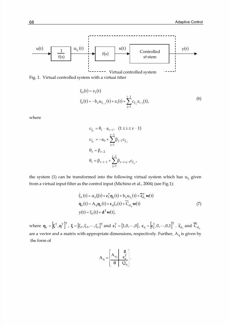
Adaptive Control68
Fig. 1. Virtual controlled system with a virtual filter
( ) ( )
( ) ( ) ( ) ( )∑−
=
−++−=
=
−
1i
1 j
jiξifzi
11
,tzctztubtξ
tztξ
j1i
(6)
where
( )
∑
∑
−
=
−+−−−
−
−
=
−
−
+=
=
+−=
−≤≤−=
1i
1 j
ξ1 jir1iri
2r1
1r
1 j
ξ1 j0ξ
iriξ
,cββθ
βθ
cβac
1ri1,aθc
j
jr
i
the system (1) can be transformed into the following virtual system which has1f
u given
from a virtual input filter as the control input (Michino et al., 2004) (see Fig.1):
( ) ( ) ( ) ( ) ( )
( ) ( ) ( ) ( )
( ) ( ) ( ),ttξty
tCtξtAt
ttubttξαtξ
T1
d1ηyηy
Tdfzy
T1z1
η
11
wd
wcηη
wcηc
+=
++=
+++=
&
&
(7)
where [ ] [ ]Tr32
TTTy ξ,,ξ,ξ,, L== ξ ηξ η and [ ] [ ]TT
ξηT1 1,0,,0,,0,,0,1 LL ccc == .
1dc andηdC
are a vector and a matrix with appropriate dimensions, respectively. Further, ηA is given by
the form of
.Q
AA
η
Tz
uη
f
⎥⎥⎥
⎦
⎤
⎢⎢⎢
⎣
⎡
=0
c
0
)s(f
1( )sf
Controlleds stem
( )tu ( )tu1f
( )tu ( )ty
Virtual controlled system
Adaptive output regulation of unknown linear systems with unknown exosystems 69
SincefuA and ηQ are stable matrices, ηA is a stable matrix.
3.2 Virtual error systemNow, consider a stable filter of the form:
( ) ( ) ( )
( ) ( ) ( ) ,tuttu
tutAt
1f
1ffff
fcT
f
fcccc
+=
+=
zθ
czz&(8)
where [ ]Tc 1,0,,0
fL=c and
[ ].βα,,βα
β,,βA
1m0
1m0f
c1mc0T
cc
1m1mc
−
−
−−=
⎥⎦
⎤⎢⎣
⎡
−−=
−
−×−
L
L
θ
I0
1m10 ccc β,,β,β−
L are chosen such thatfcA is stable.
Let's consider transforming the system (7) into a one with uf given in (8) as the input. Definenew variables X1 and 2X as follows:
.ααα
ξαξαξαξX
y0y1)1m(
y1m)m(
y2
1011)1m(
11m)m(
11
ηηηηX ++++=
++++=
−−
−−
&L
&L
(9)
Since it follows from the Cayley-Hamilton theorem that
,0IαAαAαA 0m11m
m1mmm =++++ −
− L (10)
we have from (2) and (7) that
( ) ( ) ( ) ( )
( ) ( ) ( ),tXtAt
tubttXαtX
1η2η2
fz2T11z1
cXX
Xc
+=
++=
&
&
(11)
where
1111 f0f1)1m(
f1m)m(
ff uαuαuαuu ++++= −− &L (12)
Further we have from (10) that
.Xeαeαeαe 101)1m(
1m)m( =++++ −
− &L (13)
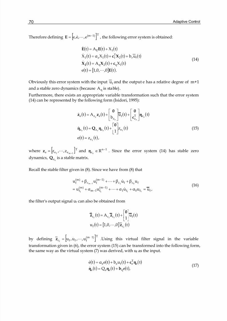
Adaptive Control70
Therefore defining [ ]T)1(me,,ee, −= L&E , the following error system is obtained:
( ) ( ) ( )
( ) ( ) ( ) ( )
( ) ( ) ( )
( ) [ ] ( ).t0,,0,1te
tXtAt
tubttXαtX
tXtAt
1η2η
fz2T11z1
1E
E
cXX
Xc
EE
2
L
&
&
&
=
+=
++=
+=
(14)
Obviously this error system with the input fu and the output e has a relative degree of m+1
and a stable zero dynamics (because ηA is stable).
Furthermore, there exists an appropriate variable transformation such that the error system(14) can be represented by the following form (Isidori, 1995):
( ) ( ) ( ) ( )
( ) ( ) ( )
( ) ( ) ,tzte
tz1
tt
ttub
tAt
1
1eee
e
ee
e
e
ezzz
zTz
fz
eze
=
⎥⎦
⎤⎢⎣
⎡+=
⎥⎦
⎤⎢⎣
⎡+⎥
⎦
⎤⎢⎣
⎡+=
0ηQη
ηc
00zz
&
&
(15)
where [ ]Teee 1m1
z,,z+
= Lz and 1nz R
e
−∈η . Since the error system (14) has stable zero
dynamics,ezQ is a stable matrix.
Recall the stable filter given in (8). Since we have from (8) that
,uuαuαuαu
uβuβuβu
ff0f1)1m(
f1m)m(
f
fcfc)1m(
fc)m(
f
1111
011m
=++++=
++++
−−
−−
&L
&L
(16)
the filter's output signal uf can also be obtained from
( ) ( ) ( )
( ) [ ] ( )t0,,0,1tu
tu1
tAt
f
fff
cf
fccc
z
0zz
L
&
=
⎥⎦
⎤⎢⎣
⎡+=
by defining [ ]T)1m(fffc u,,u,u
f
−= L&z .Using this virtual filter signal in the variable
transformation given in (6), the error system (15) can be transformed into the following form,the same way as the virtual system (7) was derived, with uf as the input.
( ) ( ) ( ) ( )
( ) ( ) ( ),tetQt
ttubteαte
ηeee
eTefee
bηη
ηc
+=
++=
&
&
(17)
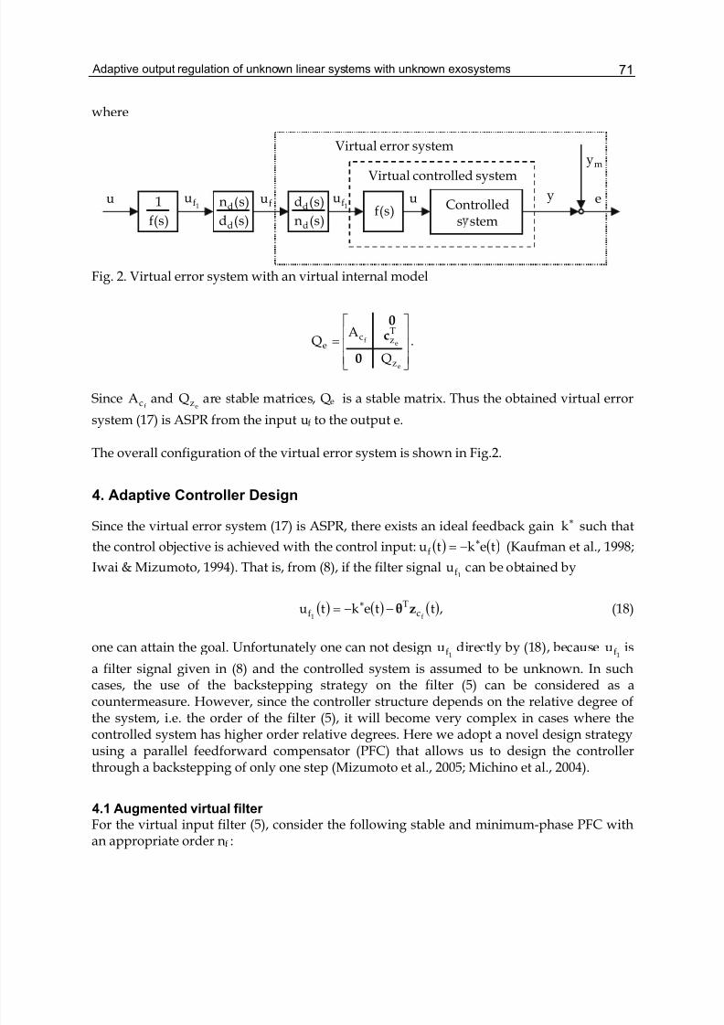
Adaptive output regulation of unknown linear systems with unknown exosystems 71
where
Fig. 2. Virtual error system with an virtual internal model
.
Q
AQ
e
ef
z
Tzc
e
⎥⎥⎥
⎦
⎤
⎢⎢⎢
⎣
⎡
=
0
c0
SincefcA and
ezQ are stable matrices, Qe is a stable matrix. Thus the obtained virtual error
system (17) is ASPR from the input uf to the output e.
The overall configuration of the virtual error system is shown in Fig.2.
4. Adaptive Controller Design
Since the virtual error system (17) is ASPR, there exists an ideal feedback gain ∗k such that
the control objective is achieved with the control input: ( ) ( )tektuf∗−= (Kaufman et al., 1998;
Iwai & Mizumoto, 1994). That is, from (8), if the filter signal1f
u can be obtained by
( ) ( ) ( ),ttektuf1 c
Tf zθ−−= ∗ (18)
one can attain the goal. Unfortunately one can not design1f
u directly by (18), because1f
u is
a filter signal given in (8) and the controlled system is assumed to be unknown. In suchcases, the use of the backstepping strategy on the filter (5) can be considered as acountermeasure. However, since the controller structure depends on the relative degree ofthe system, i.e. the order of the filter (5), it will become very complex in cases where thecontrolled system has higher order relative degrees. Here we adopt a novel design strategyusing a parallel feedforward compensator (PFC) that allows us to design the controllerthrough a backstepping of only one step (Mizumoto et al., 2005; Michino et al., 2004).
4.1 Augmented virtual filter
For the virtual input filter (5), consider the following stable and minimum-phase PFC withan appropriate order nf :
u
)s(f
1 1fu
)s(n
)s(d
d
d
)s(d
)s(n
d
d fu1f
u)s(f
u y
my
eControlleds stem
Virtual controlled system
Virtual error system
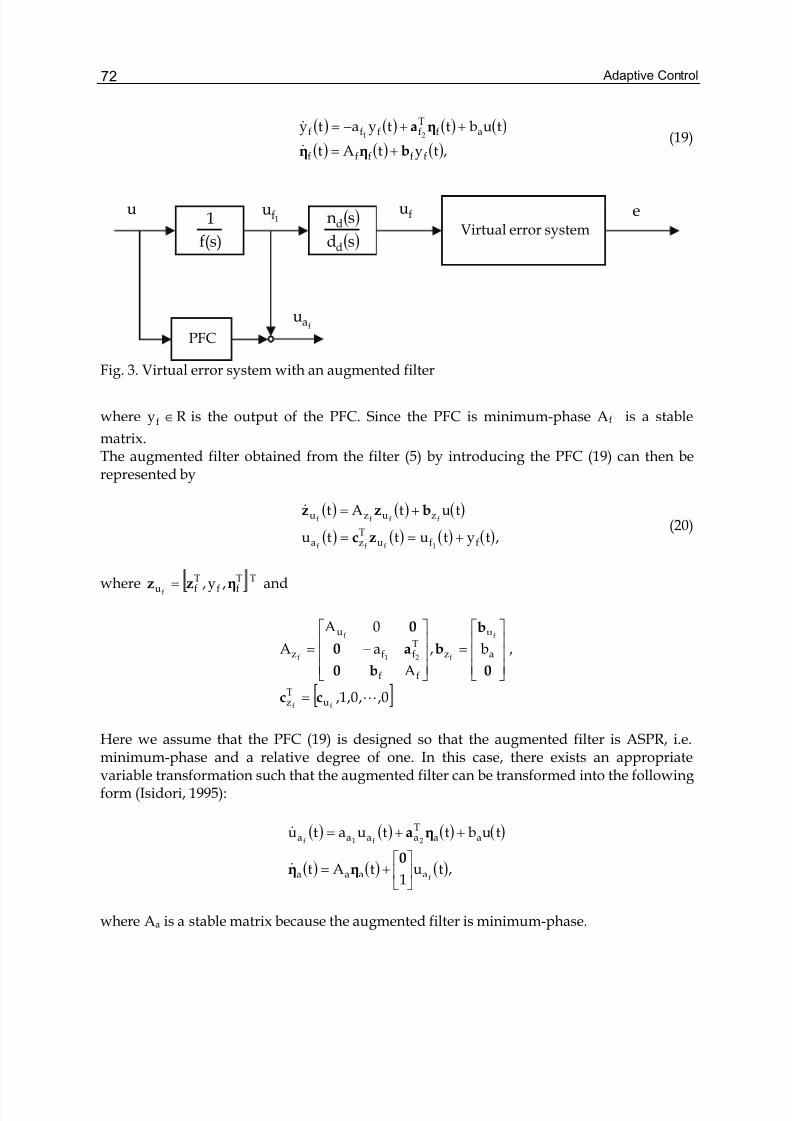
Adaptive Control72
( ) ( ) ( ) ( )
( ) ( ) ( ),tytAt
tubttyaty
fffff
afTffff 21
bηη
ηa
+=
++−=
&
&
(19)
Fig. 3. Virtual error system with an augmented filter
where Ryf ∈ is the output of the PFC. Since the PFC is minimum-phase Af is a stable
matrix.The augmented filter obtained from the filter (5) by introducing the PFC (19) can then berepresented by
( ) ( ) ( )
( ) ( ) ( ) ( ),tytuttu
tutAt
ffuTza
zuzu
1fff
ffff
+==
+=
zc
bzz&(20)
where TTff
Tfu ,y,
fηzz = and
[ ]0,,0,1,
,b,
A
a
0A
A
ff
f
f21
f
f
uTz
a
u
z
ff
Tff
u
z
Lcc
0
b
b
b0
a0
0
=
⎥⎥⎥
⎦
⎤
⎢⎢⎢
⎣
⎡
=
⎥⎥⎥
⎦
⎤
⎢⎢⎢
⎣
⎡
−=
Here we assume that the PFC (19) is designed so that the augmented filter is ASPR, i.e.minimum-phase and a relative degree of one. In this case, there exists an appropriatevariable transformation such that the augmented filter can be transformed into the followingform (Isidori, 1995):
( ) ( ) ( ) ( )
( ) ( ) ( ),tu1
tAt
tubttuatu
f
2f1f
aaaa
aaTaaaa
⎥⎦
⎤⎢⎣
⎡+=
++=
0ηη
ηa
&
&
where Aa is a stable matrix because the augmented filter is minimum-phase.
)s(f
1 ( )
( )sd
sn
d
d Virtual error system
u1f
u fu e
PFCfau
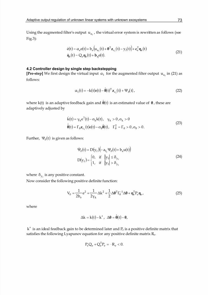
Adaptive output regulation of unknown linear systems with unknown exosystems 73
Using the augmented filter's outputfau , the virtual error system is rewritten as follows (see
Fig.3):
( ) ( ) ( ) ( ) ( )( ) ( )
( ) ( ) ( ).tetQt
ttyttubteαte
ηeee
eTefc
Taee ff
bηη
ηczθ
+=
+−++=
&
&
(21)
4.2 Controller design by single step backstepping [Pre-step] We first design the virtual input 1α for the augmented filter output
fau in (21) as
follows:
( ) ( ) ( ) ( ) ( ) ( ) ,tΨttˆtetktα 0cT
1 f+−−= zθ (22)
where k(t) is an adaptive feedback gain and ( )tθ is an estimated value of θ , these are
adaptively adjusted by
( ) ( ) ( )
( ) ( ) ( ) ( ) .0σ,0ΓΓ,tˆσtetΓtˆ
0σ,0γ,tkσteγtk
θθTθθcθ
kkk2
k
f>>=−=
>>−=
θzθ&
&
(23)
Further, ( )tΨ0 is given as follows:
( ) ( ) ( ) ( )( )
( )⎪⎩
⎪⎨⎧
>
≤=
+−=
f
f
1
yf
yff
a0ff0
δyif,1
δyif,0yD
tubtΨayDtΨ&
(24)
wherefyδ is any positive constant.
Now consider the following positive definite function:
,PΔΓΔ2
1kΔ
γ2
1e
b2
1V ee
Te
1θ
T2
k
2
e0 ηηθθ +++= − (25)
where
( ) ( ) ,tˆΔ,ktkkΔ θθθ −=−= ∗
∗k is an ideal feedback gain to be determined later and Pe is a positive definite matrix that
satisfies the following Lyapunov equation for any positive definite matrix Re.
.0RPQQP eeTeee <−=+
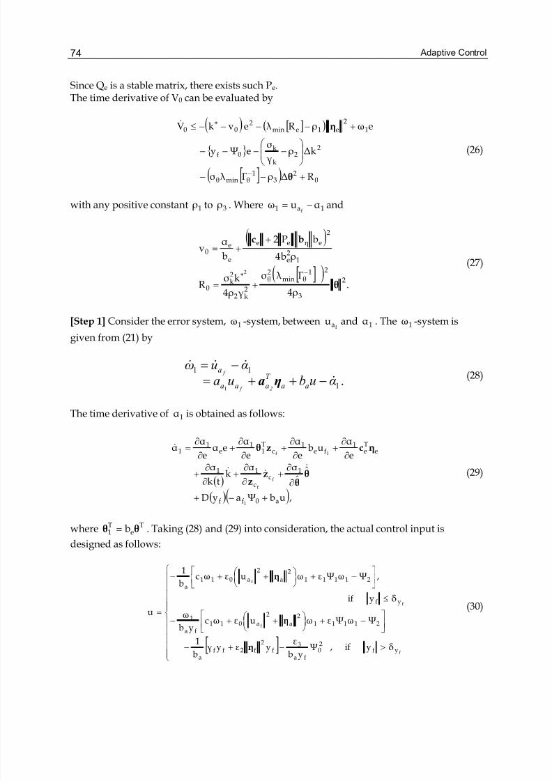
Adaptive Control74
Since Qe is a stable matrix, there exists such Pe.The time derivative of V0 can be evaluated by
( ) [ ]( )
[ ]( ) 02
31
θminθ
22
k
k0f
12
e1emin2
00
RΔρΓ λσ
kΔργ
σeΨy
eωρR λevkV
+−−
⎟⎟ ⎠
⎞⎜⎜⎝
⎛ −−−−
+−−−−≤
−
∗
θ
η&
(26)
with any positive constant 1ρ to 3ρ . Where 1a1 αuωf−= and
( )
[ ]( ).
ρ4
Γ λσ
γρ4
kσR
ρb4
bP2
b
αv
2
3
21θmin
2θ
2k2
2k
0
12e
2
eηee
e
e0
2
θ
bc
−∗
+=
++=
(27)
[Step 1] Consider the error system, 1ω -system, betweenfau and 1α . The 1ω -system is
given from (21) by
.1
11
1
αubua
αuω
aa
T
aaa
a
2 f
f
&
&&&
−++=−=
ηa(28)
The time derivative of 1α is obtained as follows:
( )
( )( ),ubΨayD
ˆˆαα
ktk
αe
αub
e
α
e
αeα
e
αα
a0ff
1c
c
11
eTe
1fe
1c
T1
1e
11
1
f
f
1f
+−+
∂
∂+
∂
∂+
∂
∂+
∂
∂+
∂
∂+
∂
∂+
∂
∂=
θθ
zz
ηczθ
&&&
&
(29)
where Te
T1 b θθ = . Taking (28) and (29) into consideration, the actual control input is
designed as follows:
[ ]⎪⎪⎪⎪⎪
⎩
⎪⎪⎪⎪⎪
⎨
⎧
>−+−
⎥⎦
⎤⎢⎣
⎡−+⎟
⎠ ⎞
⎜⎝ ⎛ ++−
≤
⎥⎦
⎤⎢⎣
⎡−+⎟
⎠ ⎞
⎜⎝ ⎛ ++−
=
f
f
f
f
yf20
fa
3f
2f2ff
a
211112
a
2
a011fa
1
yf
211112
a
2
a011a
δyif,Ψyb
εyεyγ
b
1
ΨωΨεωuεωcyb
ω
δyif
,ΨωΨεωuεωcb
1
u
η
η
η
(30)
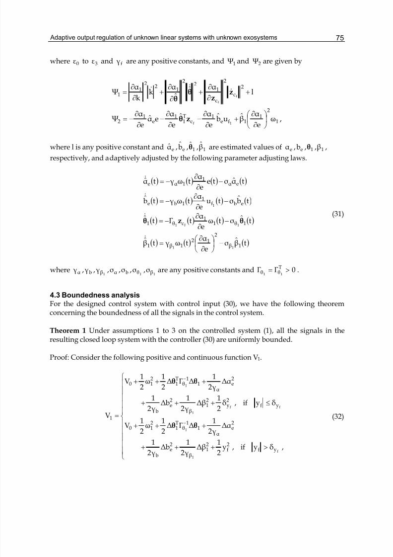
Adaptive output regulation of unknown linear systems with unknown exosystems 75
where 0ε to 3ε and fγ are any positive constants, and 1Ψ and 2Ψ are given by
,ωe
αβub
e
αˆe
αeα
e
αΨ
lαˆ
ˆα
kk
αΨ
1
21
1fe1
cT1
1e
12
2
c
2
c
12
2
12
21
1
1f
f
f
⎟ ⎠
⎞⎜⎝
⎛
∂
∂+
∂
∂−
∂
∂−
∂
∂−=
+∂
∂+
∂
∂+
∂
∂=
zθ
zz
θθ
&&&
where l is any positive constant and 11ee β,ˆ,b,α θ are estimated values of 11ee β,,b,α θ ,
respectively, and adaptively adjusted by the following parameter adjusting laws.
( ) ( ) ( ) ( )
( ) ( ) ( ) ( )
( ) ( ) ( ) ( )
( ) ( ) ( )tβσe
αtωγtβ
tˆσtωe
αtΓtˆ
tbσtue
αtωγtb
tασtee
αtωγtα
1β
212
1β1
1θ11
cθ1
ebf1
1be
eα1
1αe
11
1f1
1
−⎟ ⎠
⎞⎜⎝
⎛
∂
∂=
−∂
∂−=
−∂
∂−=
−∂
∂−=
&
&
&
&
θzθ(31)
where111 βθbαβbα σ,σ,σ,σ,γ,γ,γ are any positive constants and 0ΓΓ T
θθ 11>= .
4.3 Boundedness analysis For the designed control system with control input (30), we have the following theoremconcerning the boundedness of all the signals in the control system.
Theorem 1 Under assumptions 1 to 3 on the controlled system (1), all the signals in theresulting closed loop system with the controller (30) are uniformly bounded.
Proof: Consider the following positive and continuous function V1.
⎪⎪⎪⎪⎪
⎩
⎪⎪⎪⎪⎪
⎨
⎧
>+++
+++
≤+++
+++
=−
−
,δyif,y2
1βΔ
γ2
1bΔ
γ2
1
αΔγ2
1ΔΓΔ
2
1ω
2
1V
δyif,δ2
1βΔ
γ2
1bΔ
γ2
1
αΔγ2
1ΔΓΔ
2
1ω
2
1V
V
f
1
1
ff
1
1
yf2f
21
β
2e
b
2e
α1
1θ
T1
210
yf2y
21
β
2e
b
2e
α1
1θ
T1
210
1
θθ
θθ
(32)
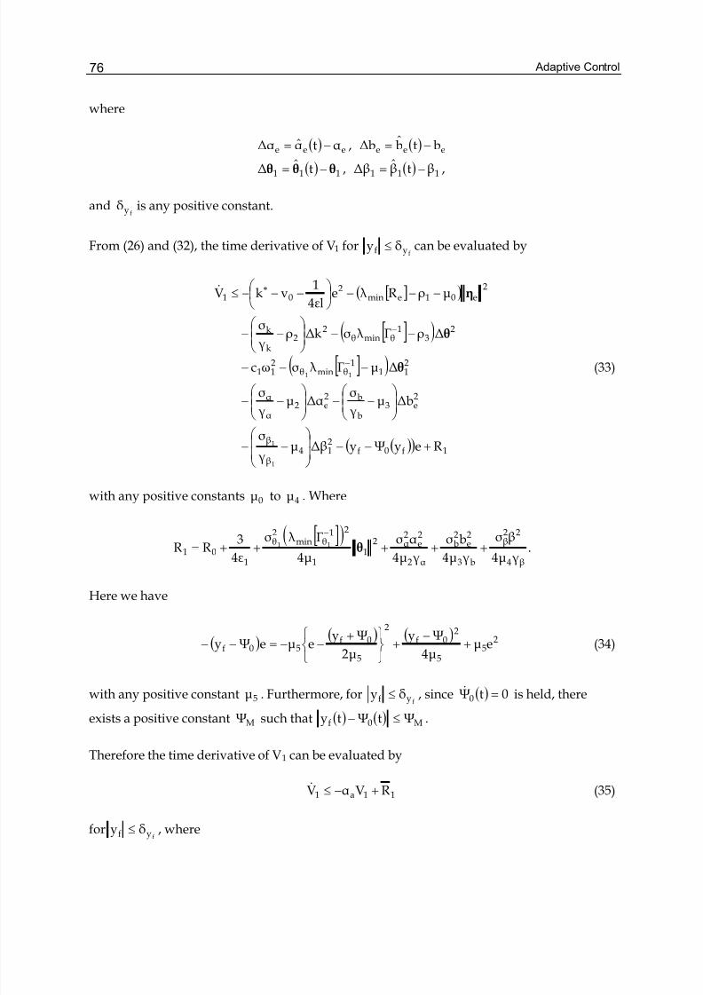
Adaptive Control76
where
( ) ( )
( ) ( ) ,βtββΔ,tˆΔ
btbbΔ,αtααΔ
111111
eeeeee
−=−=
−=−=
θθθ
andfyδ is any positive constant.
From (26) and (32), the time derivative of V1 forfyf δy ≤ can be evaluated by
[ ]( )
[ ]( )
[ ]( )
( )( ) 1f0f214
β
β
2e3
b
b2e2
α
α
211
1θminθ
211
23
1θminθ
22
k
k
2e01emin
201
ReyΨyβΔμγ
σ
bΔμγ
σαΔμ
γ
σ
ΔμΓ λσωc
ΔρΓ λσkΔργ
σ
μρR λeεl4
1vkV
1
1
11
+−−⎟⎟
⎠
⎞
⎜⎜
⎝
⎛ −−
⎟⎟ ⎠
⎞⎜⎜⎝
⎛ −−⎟
⎟ ⎠
⎞⎜⎜⎝
⎛ −−
−−−
−−⎟⎟ ⎠
⎞⎜⎜⎝
⎛ −−
−−−⎟ ⎠
⎞⎜⎝
⎛ −−−≤
−
−
∗
θ
θ
η&
(33)
with any positive constants 0μ to 4μ . Where
[ ]( ).
γμ4
βσ
γμ4
bσ
γμ4
ασ
μ4
Γ λσ
ε4
3RR
β4
22β
b3
2e
2b
α2
2e
2α2
11
21θmin
2θ
101
11 +++++=−
θ
Here we have
( )( ) ( ) 2
55
20f
2
5
0f50f eμ
μ4
Ψy
μ2
ΨyeμeΨy +
−+
⎭⎬⎫
⎩⎨⎧ +
−−=−− (34)
with any positive constant 5μ . Furthermore, forfyf δy ≤ , since ( ) 0tΨ0 =& is held, there
exists a positive constant MΨ such that ( ) ( ) M0f ΨtΨty ≤− .
Therefore the time derivative of V1 can be evaluated by
11a1 RVαV +−≤& (35)
forfyf δy ≤ , where
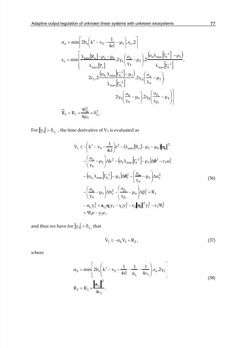
Adaptive output regulation of unknown linear systems with unknown exosystems 77
[ ]
[ ]
[ ]( )
[ ][ ]( )
[ ]
.δμ4
ΨRR
μγ
σγ2,μ
γ
σγ2
,μγ
σγ2,
Γ λ
μΓ λσ2,c2
,
Γ λ
ρΓ λσ2,ρ
γ
σγ2,
P λ
μρR λmins
2,s,μεl4
1vkb2minα
2y
5
2M
11
4β
ββ3
b
bb
2α
αα
1θmax
11
θminθ1
1θmac
31
θminθ
2k
kk
emax
01emina
a50ea
f
1
1
1
11
++=
⎥⎥
⎦
⎤
⎟⎟
⎠
⎞
⎜⎜
⎝
⎛ −⎟
⎟ ⎠
⎞⎜⎜⎝
⎛ −
⎟⎟ ⎠
⎞⎜⎜⎝
⎛ −
−
−
⎟⎟ ⎠
⎞⎜⎜⎝
⎛ −
⎢⎢⎢
⎣
⎡−−
=
⎥⎦
⎤⎢⎣
⎡⎟ ⎠
⎞⎜⎝
⎛ −−−=
−
−
−
−
∗
Forfyf δy > , the time derivative of V1 is evaluated as
[ ]( )
[ ]( )
[ ]( )
,eyeΨ
Ψεyεyγyya
RβΔμγ
σbΔμ
γ
σ
αΔμγ
σΔμΓ λσ
ωcΔρΓ λσkΔργ
σ
μρR λeεl4
1vkV
f0
203
2f
2f2
2fffff
2ff
1214
β
β2e3
b
b
2e2
α
α211
1θminθ
211
23
1θminθ
22
k
k
2e01emin
201
21
1
1
11
−+
−−−+−
+⎟⎟
⎠
⎞
⎜⎜
⎝
⎛ −−⎟
⎟ ⎠
⎞⎜⎜⎝
⎛ −−
⎟⎟ ⎠
⎞⎜⎜⎝
⎛ −−−−
−−−⎟⎟ ⎠
⎞⎜⎜⎝
⎛ −−
−−−⎟ ⎠
⎞⎜⎝
⎛ −−−≤
−
−
∗
ηηa
θ
θ
η&
(36)
and thus we have forfyf δy > that
,RVαV 21b1 +−≤& (37)
where
.4ε
RR
γ2,s,ε4
1
a
1
εl4
1vkb2minα
2
2
f
12
fa3f
0eb
2
1
a+=
⎥⎥
⎦
⎤
⎢⎢
⎣
⎡
⎟⎟
⎠
⎞
⎜⎜
⎝
⎛ −−−−= ∗
(38)
Adaptive Control78
Finally, for an ideal feedback gain ∗k which satisfies
,ε4
1
a
1,μmaxv,v
εl4
1vk
3f5110
1 ⎥⎥⎦
⎤
⎢⎢⎣
⎡−=++>∗
the time derivative of V1 can be evaluated by
,RαVV 11 +−≤& (39)
where [ ] 21ba R,RmaxR,0α,αminα =>= . Consequently it follows that V1 is uniformly
bounded and thus the signals ( ) ( ) ( ) ( ) ( )t,ty,t,tω,te ffe1 ηη and adjusted parameters ( ) ( ),tˆ,tk θ
( ) ( ) ( ) ( )tβ,tb,tˆ,tα 1e1e θ are also uniformly bounded.
Next, we show that the filter signalfcz and the control input u are uniformly bounded.
Define new variable1ξ
z as follows:
1ξc)1m(
ξc)m(
ξ ξzβzβz1011m1=+++ −
−L (40)
wcηc Tdfzy
Tξ1z1 11
ubξαξ +++=& (41)
,CξAηd1ηyηy wbηη ++=& (42)
where 1ξ and yη have been given in (7). Further define1β
z by
1f11 βczβzβ ηzbzαz ++=& (43)
,ηβηβη Tdy
Tξβc
)1m(βc
)m(β 11011m1
wcηc +=+++ −
−L (44)
where [ ]f1f cc 0,,0,1z zL= and we set ( ) ( ) m,,0k,0z0z )k(
ξ)k(
β 11L== .We have from (40) and (41)
that
( )( )
( ).ub
zαzβαβ
zβαβ
zαβzξαξ
Tdy
Tξfz
ξzξczc
)1m(ξczc
)m(ξzc
)1m(ξ1z1
11
1110
11m2m
11m1
wcηc ++=
−−+
+−+
−+=−
−
+
−−
−
&
L
&
(45)
Further, we have from (43), (44) and (8) that
Adaptive output regulation of unknown linear systems with unknown exosystems 79
( ) ( )( )
.ub
zαzβαβ
zβαβzαβz
Tdy
Tξfz
βzβczc
)1m(βczc
)m(βzc
)1m(β
11
1110
11m2m11m1
wcηc ++=
−−++
−+−+ −+−−−
&L (46)
It follows from (45) and (46) that m,,0k,zz )k(β
)k(ξ 11
L== .
Define [ ]T)1m(ξξξξ 111
z,,z,z −= L&z and [ ]T)1m(ββββ 111
z,,z,z −= L&z . Since01m c
1mc
m βsβs +++ −−
L
is a stable polynomial, we obtain from (40) that
,lξl 211ξβ +≤= zz (47)
with appropriate positive constants l1, l2. From the boundedness of ( )tw and e(t), we have
( )tξ1 is bounded and thus βz is also bounded.
Furthermore defining [ ]T)1m(ββββ 111
η,,η,η −= L&η , we have from (44) that
( ) ( ) ( ) ( )( ).tt1
tAt Tdy
Tξβcβ 1f
wcηc0
ηη +⎥⎦
⎤⎢⎣
⎡+=& (48)
From (8) and (48), we obtain
( ) ( )
( ) ( )( ) ( ) ( ) ( )( ).tt1
tu1
bttbA
ttb
Tdy
Tξfzβczc
βcz
11ff
f
wcηc00
ηz
ηz
+⎥⎦
⎤⎢⎣
⎡+⎥
⎦
⎤⎢⎣
⎡++=
+ &&
(49)
Therefore ( ) ( )ttb βcz fηz && + can be evaluated from (48) and the fact that f11f yαωu
1−+= by
( ) ( ) ( ) ( )
( ) ( ) ( )
( ) ( ) .tt
tωbtytαb
ttbAttb
1
fff
dyξ
1zf1z
βczcβcz
wcηc
ηzηz
++
+−+
+≤+ &&
(50)
Here, we have from (22) that
( ) ( ) ( ) ( )( )
( ) ( ) ( )( ) ( ) ( ).tyyΨt
b
tˆttb
b
tˆtetktytα ff0β
z
T
βczz
T
f1 f−+++−−=− η
θηz
θ(51)
Adaptive Control80
Since it follows from (19) and (24) that
( ) ( ) ( ) ( )( ) ( )ttΨtyatΨty fTf0ff0f 21ηa+−−=− && (52)
forfyf δy > and from the boundedness of ( )tfη , there exists a positive constant such that
( ) M0f ΨtΨy ≤− . Further, from the boundedness of ( )tw and e(t) i.e. ( )tξ1 , we can confirm
that ( )tyη and ( )tβη are also bounded from (7) and (48). Finally, taking the boundedness of
the signals e(t), ( ) ( ) ( )tˆ,tk,tω1 θ and ( ) ( )t,t βy ηη into consideration, from (50) ( ) ( )ttb βcz fηz && + can
be evaluated by
( ) ( ) ( ) ( )2f1f zβczzβcz lttblttb ++≤+ ηzηz && (53)
with appropriate positive constants1zl and
2zl . Consequently, considering the system:
( ) ( )tbαt βczβzβ fηzzz ++=& (54)
from (44) with ( )tb βcz fηz + as the input and βz as the output, since this system is
minimum-phase and the inequality (53) is held, we have from the Output/Input Lp Stability
Lemma (Sastry & Bodson, 1989) that the input ( )tb βcz fηz + in the system (54) can be
evaluated by
( ) ( ) ( )21f zβzβcz ltlttb +≤+ zηz (55)
with appropriate positive constants1zl and
2zl . From the boundedness of ( )tβz and ( )tβη ,
we can conclude that ( )tfcz is uniformly bounded and then the control input u(t) is also
uniformly bounded. Thus all the signals in the resulting closed loop system with thecontroller (30) are uniformly bounded.
5. Simulation Results
The effectiveness of the proposed method is confirmed through numerical simulation for a3rd order SISO system with a relative degree of 3, which is given by
[ ] ,1.011.01.0zy
1
1.0
1.0
1.0
1
1.0
1.0
1.0
1.0
1.0
1.0
1
u
1
0
0
15.02.5
5.05.21.5
5.05.01
1 w
wzz
+=
⎥⎥⎥
⎦
⎤
⎢⎢⎢
⎣
⎡
+
⎥⎥⎥
⎦
⎤
⎢⎢⎢
⎣
⎡
+
⎥⎥⎥
⎦
⎤
⎢⎢⎢
⎣
⎡
−
−−
−−
=&(56)
where w is an unknown disturbance which has the following form:
Adaptive output regulation of unknown linear systems with unknown exosystems 81
( )
( )
( )
( )⎥⎥⎥⎥⎥
⎦
⎤
⎢⎢⎢⎢⎢
⎣
⎡
=
t5cos5.2
t5sin5.0
t2cos2
2tsin
w (57)
Before designing a controller, we first introduce the following pre-filter:
as
b
+(58)
in order to reduce the chattering phenomenon to be expected by switching the controllergiven in (30). Therefore, the considered controlled system has a relative degree of 4.
Since the relative degree of the controlled system is 4, we consider a 3rd order input virtualfilter in (5). Further we consider a stable internal model filter (8) of the order of 4.
For the input virtual filter, in this simulation, we consider a first order PFC:
ubyay afff 1+−=&
in order to make an ASPR augmented filter.
The design parameters for the pre-filter (58), the input virtual filter (5) and the internalmodel filter (8) are set as follows:
625β,500β,150β,20β
125β,75β,15β
1000ba
3210 cccc
210
====
===
==
and the PFC parameters are set by
.01.0b,10a af1==
Further design parameters in the controller given in (23), (24), (30) and (31) are designed by
.100γε,01.0εεε,1000c
100γγγ,I5000ΓΓ
1.0σσσσ,05.0σ,5.0l
10δ,01.0σ,500γ
f32101
βba4θθ
βbaθθ
ykk
1
11
f
======
=====
======
===
Figure 4 shows the simulation results with the proposed controller. In this simulation, thedisturbance w is changed at 50 [sec]:
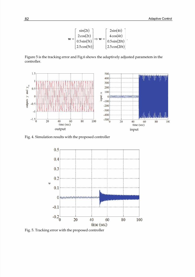
Adaptive Control82
input output
( )
( )
( )
( )
( )
( )
( )
( )
.
t20cos5.2
t20sin5.0
t4cos4
t4sin2
t5cos5.2
t5sin5.0
t2cos2
2tsin
⎥⎥⎥⎥⎥
⎦
⎤
⎢⎢⎢⎢⎢
⎣
⎡
=⇒
⎥⎥⎥⎥⎥
⎦
⎤
⎢⎢⎢⎢⎢
⎣
⎡
= ww
Figure 5 is the tracking error and Fig.6 shows the adaptively adjusted parameters in thecontroller.
Fig. 4. Simulation results with the proposed controller
Fig. 5. Tracking error with the proposed controller
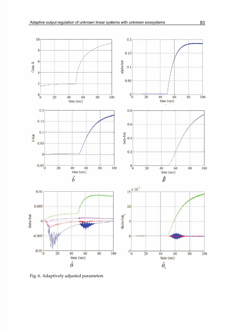
Adaptive output regulation of unknown linear systems with unknown exosystems 83
Fig. 6. Adaptively adjusted parameters
feedback gain k(t) α
b ˆ
θ 1θ
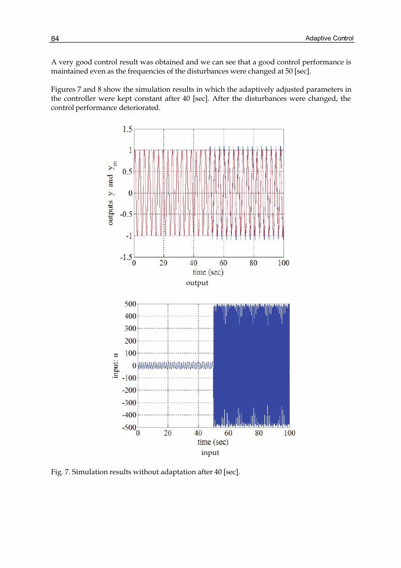
Adaptive Control84
A very good control result was obtained and we can see that a good control performance ismaintained even as the frequencies of the disturbances were changed at 50 [sec].
Figures 7 and 8 show the simulation results in which the adaptively adjusted parameters inthe controller were kept constant after 40 [sec]. After the disturbances were changed, thecontrol performance deteriorated.
Fig. 7. Simulation results without adaptation after 40 [sec].
input
output
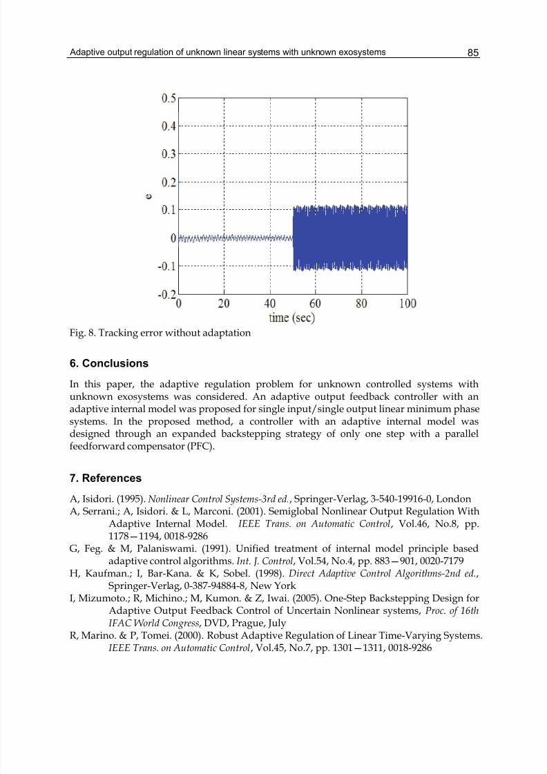
Adaptive output regulation of unknown linear systems with unknown exosystems 85
Fig. 8. Tracking error without adaptation
6. Conclusions
In this paper, the adaptive regulation problem for unknown controlled systems withunknown exosystems was considered. An adaptive output feedback controller with anadaptive internal model was proposed for single input/single output linear minimum phasesystems. In the proposed method, a controller with an adaptive internal model wasdesigned through an expanded backstepping strategy of only one step with a parallelfeedforward compensator (PFC).
7. References
A, Isidori. (1995). Nonlinear Control Systems-3rd ed., Springer-Verlag, 3-540-19916-0, LondonA, Serrani.; A, Isidori. & L, Marconi. (2001). Semiglobal Nonlinear Output Regulation With
Adaptive Internal Model. IEEE Trans. on Automatic Control, Vol.46, No.8, pp.1178—1194, 0018-9286
G, Feg. & M, Palaniswami. (1991). Unified treatment of internal model principle basedadaptive control algorithms. Int. J. Control, Vol.54, No.4, pp. 883—901, 0020-7179
H, Kaufman.; I, Bar-Kana. & K, Sobel. (1998). Direct Adaptive Control Algorithms-2nd ed.,Springer-Verlag, 0-387-94884-8, New York
I, Mizumoto.; R, Michino.; M, Kumon. & Z, Iwai. (2005). One-Step Backstepping Design forAdaptive Output Feedback Control of Uncertain Nonlinear systems, Proc. of 16thIFAC World Congress, DVD, Prague, July
R, Marino. & P, Tomei. (2000). Robust Adaptive Regulation of Linear Time-Varying Systems.IEEE Trans. on Automatic Control, Vol.45, No.7, pp. 1301—1311, 0018-9286
Adaptive Control86
R, Marino. & P, Tomei. (2001). Output Regulation of Linear Systems with Adaptive InternalModel, Proc. of the 40th IEEE CDC , pp. 745—749, 0-7803-7061-9, USA, December,Orlando, Florida
R, Michino.; I, Mizumoto.; M, Kumon. & Z, Iwai. (2004). One-Step Backstepping Design ofAdaptive Output Feedback Controller for Linear Systems, Proc. of ALCOSP 04, pp.705-710, Yokohama, Japan, August
S, Sastry. & M, Bodson. (1989). Adaptive Control Stability, Convergence, and Robustness,Prentice Hall, 0-13-004326-5
V, O, Nikiforov. (1996). Adaptive servocompensation of input disturbances, Proc. of the 13thIFAC World Congress, Vol.K, pp. 175—180, San-Francisco
V, O, Nikiforov. (1997a). Adaptive servomechanism controller with implicit reference model.Int J. Control, Vol.68, No.2, pp. 277—286, 0020-7179
V, O, Nikiforov. (1997b). Adaptive controller rejecting uncertain deterministic disturbancesin SISO systems, Proc. of European Control Conference, Brussels, Belgium
Z, Ding. (2001). Global Output Regulation of A Class of Nonlinear Systems with UnknownExosystems, Proc. of the 40th IEEE CDC , pp. 65—70, 0-7803-7061-9, USA, December,Orlando, Florida
Z, Iwai. & I, Mizumoto. (1994). Realization of Simple Adaptive Control by Using ParallelFeedforward Compensator. Int. J. Control, Vol.59, No.6, pp. 1543—1565, 0020-7179
4
Output Feedback Direct Adaptive Controlfor a Two-Link Flexible Robot Subject to
Parameter Changes
Selahattin Ozcelik and Elroy MirandaTexas A&M University-Kingsville, Texas
USA
1. Introduction
Robots today have an ever growing niche. Many of today’s robots are required to performtasks which demand high level of accuracy in end effector positioning. The links of the robotconnecting the joints are large, rigid, and heavy. These manipulators are designed withlinks, which are sufficiently stiff for structural deflection to be negligible during normaloperation. Also, heavy links utilize much of the joint motor’s power moving the link andholding them against gravity. Moreover the payloads have to be kept small compared to themass of the robot itself, since large payloads induce sagging and vibration in the links,eventually bringing about uncertainty in the end effector position. In an attempt to solvethese problems lightweight and flexible robots have been developed. These lightweightmechanical structures are expected to improve performance of the robot manipulators withtypically low payload to arm weight ratio. The ultimate goal of such robotic designs is toaccurate tip position control in spite of the flexibility in a reasonable amount of time. Unlikeindustrial robots, these robot links will be utilized for specific purposes like in a spaceshuttle arm. These flexible robots have an increased payload capacity, lesser energyconsumption, cheaper construction, faster movements, and longer reach. However, linkflexibility causes significant technical problems. The weight reduction leads the manipulatorto become more flexible and more difficult to control accurately. The manipulator being adistributed parameter system, it is highly non-linear in nature. Control algorithms will berequired to compensate for both the vibrations and static deflections that result from theflexibility. This provides a challenge to design control techniques that:
a) gives precise control of desired parameters of the system in desired time,b) cope up with sudden changes in the bounded system parameters,c) gives control on unmodeled dynamics in the form of perturbations, andd) robust performance.
Conventional control system design is generally a trial and error process which is often notcapable of controlling a process, which varies significantly during operation. Thus, the questfor robust and precise control led researchers to derive various control theories. Adaptivecontrol is one of these research fields that is emerging as timely and important class ofcontroller design. Area much argued about adaptive control is its simplicity and ease of
Adaptive Control88
physical implementation on actual real-life systems. In this work, an attempt has been madeto show the simplicity, ease and effectiveness of implementation of direct model referenceadaptive control (DMRAC) on a multi input multi output (MIMO) flexible two-link system.The plant comprises of a planar two-link flexible arm with rotary joints subject only tobending deformations in the plane of motion. A payload is added at the tip of the outer link,while hub inertias are included at actuated joints. The goal is to design a controller that cancontrol the distal end of the flexible links.Probably the first work done pertaining to the control of flexible links was presented by(Cannon & Schmitz, 1984). Considering a flexible link, which was only flexible in onedimension (perpendicular to gravity), a Linear Quadratic Gaussian controller was designedfor the position control. Direct end point sensing was used and the goal was to execute arobot motion as fast as possible without residual vibrations in the beam. Also, experimentswere carried out on end point control of a flexible one link robot. These experimentsdemonstrated control strategies for position of one end to be sensed and preciselypositioned by applying torque at the other end. These experiments were performed touncover and solve problems related to the control of very flexible manipulators, wheresensors are collocated with the actuators.(Geniele et al., 1995) worked on tip-position control of a single flexible link, which rotates ona horizontal plane. The dynamic model was derived using assumed-modes method basedon the Euler-Bernoulli beam theory. The model is then linearized about an operating point.The control strategy for this non-minimum phase linear time varying system consisted oftwo parts. The first part had an inner stabilizing control loop that incorporates afeedforward term to assign the system’s transmission zeros at desired locations in thecomplex plane, and a feedback term to move the system’s poles to the desire positions in theleft half plane. In the second part, the other loop had a feedback servo loop that allowedtracking of the desired trajectory. The controller was implemented on an experimental testbed. The performance was then compared with that of a pole placement state feedbackcontroller.(Park & Asada, 1992) worked on an integrated structure and control design of a two-linknon-rigid robot arm for the purpose of high speed positioning. A PD control system wasdesigned for the simple dynamic model minimizing the settling time. Optimal feedbackgains were obtained as functions of structural parameters involved in the dynamic model.These parameters were then optimized using an optimization technique for an overalloptimal performance.(Lee et al., 2001) worked on the adaptive robust control design for multi-link flexible robots.Adaptive energy-based robust control was presented for both close loop stability andautomatic tuning of the gains for desired performance. A two-link finite element model wassimulated, in which each link was divided into four elements of same length. The controllerdesigned was independent of system parameters and hence possessed stability robustnessto parameter variations.Variations in flexible links have also been researched. Control of a two-link flexible arm incontact with a compliant surface was shown in (Scicliano & Villani, 2001). Here, for a giventip position and surface stiffness, the joint and deflection variables are computed usingclosed loop inverse kinematics algorithm. The computed variables are then used as the setpoints for a simple joint PD control, thus achieving regulation of the tip position and contactforce via a joint-space controller.
Output Feedback Direct Adaptive Control for a Two-Link Flexible Robot Subject toParameter Changes
89
(Ider et al., 2002) proposed a new method for the end effector trajectory tracking control ofrobots with flexible links. In order to cope with the non-minimum phase property of thesystem, they proposed to place the closed-loop poles at desire locations using full statefeedback. A composite control law was designed to track the desired trajectory, while at thesame time the internal dynamics were stabilized. A two-link planar robot was simulated toillustrate the performance of the proposed algorithm. Moreover the method is valid for alltypes of manipulators with any degree of freedom.(Green, A. & Sasiadek, J., 2004) presented control methods for endpoint tracking of a two-link robot. Initially, a manipulator with rigid links is modeled using inverse dynamics, alinear quadratic regulator and fuzzy logic schemes actuated by a Jacobian transpose controllaw computed using dominant cantilever and pinned-pinned assumed mode frequencies.The inverse dynamics model is pursued further to study a manipulator with flexible linkswhere nonlinear rigid-link dynamics are coupled with dominant assumed modes forcantilever and pinned-pinned beams. A time delay in the feedback control loop representselastic wave travel time along the links to generate non-minimum phase response.
An energy-based nonlinear control for a two-link flexible manipulator wasstudied in (Xu etal., 2005). It was claimed that their method can provide more physical insights in nonlinearcontrol as well as provide a direct candidate for the Lyapunov function. Both simulation andexperimental results were provided to demonstrate the effectiveness of the controllersA robust control method of a two-link flexible manipulator with neural networks basedquasi-static distortion compensation was proposed in (Li et al., 2005). The dynamicsequation of the flexible manipulator was divided into a slow subsystem and a fastsubsystem based on the assumed mode method and singular perturbation theory. Adecomposition based robust controller is proposed with respect to the slow subsystem, and
∞H control is applied to the fast subsystem. The proposed control method has been
implemented on a two-link flexible manipulator for precise end-tip tracking control.In this work a direct adaptive controller is designed and the effectiveness of this adaptivecontrol algorithm is shown by considering the parametric variations in the form of additiveperturbations. This work emphasizes the robust stability and performance of adaptivecontrol, in the presence of parametric variations. This approach is an output feedbackmethod, which requires neither full state feedback nor adaptive observers. Other importantproperties of this class of algorithms include:
a) Their applicability to non-minimum phase systems,b) The fact that the plant (physical system) order may be much higher than the
order of the reference model, andc) The applicability of this approach to MIMO systems.
Its ease of implementation and inherent robustness properties make this adaptive controlapproach attractive.
2. Mathematical Modeling of the System
In this section mathematical model of the system is derived using Lagrange equations withthe assumed-modes method. The links are assumed to obey Euler-Bernoulli beam modelwith proper boundary conditions. A payload has been added to the tip of the second link,while hub inertias are included at the actuator joints.
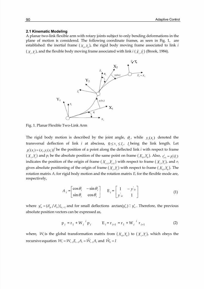
Adaptive Control90
2.1 Kinematic ModelingA planar two-link flexible arm with rotary joints subject to only bending deformations in theplane of motion is considered. The following coordinate frames, as seen in Fig. 1, areestablished: the inertial frame (
0 0, X Y ), the rigid body moving frame associated to link i
( ,i i X Y ), and the flexible body moving frame associated with link i ( ˆ ˆ,i i X Y ) (Brook, 1984).
Fig. 1. Planar Flexible Two-Link Arm
The rigid body motion is described by the joint angle,iθ , while ( )i i y x denoted the
transversal deflection of link i at abscissa, 0 i il ≤ ≤ ,i
l being the link length. Let
( ) ( , ( ))i T
i i i i i p x x y x= be the position of a point along the deflected link i with respect to frame
( ,i i X Y ) and pi be the absolute position of the same point on frame (0 0, X Y ). Also,
1( )i i
i i ir p l + =
indicates the position of the origin of frame (1 1,i i X Y + +
) with respect to frame ( ,i i X Y ), and r i
gives absolute positioning of the origin of frame ( ,i i X Y ) with respect to frame (0 0, X Y ). The
rotation matrix Ai for rigid body motion and the rotation matrix Ei for the flexible mode are,respectively,
A i = ⎥⎦
⎤⎢⎣
⎡ −
ii
ii
θ θ
θ θ
cossin
sincos E i = ⎥
⎦
⎤⎢⎣
⎡ −
1
1'
'
ie
ie
y
y (1)
where δ δ =′ = ( / )|
i iie yi xi x ly and for small deflections ′ ′arctan( )ie iey y . Therefore, the previous
absolute position vectors can be expressed as,
pi
= r1
+ Wi
ip
iE i = r
1i+ = r1
+ Wi
ir
1i+ (2)
where, iW is the global transformation matrix from (0 0, X Y ) to ( ,
i i X Y ), which obeys the
recursive equation − − −= =1 1 1ˆ
i i i i i iW W E A W A and =0W I
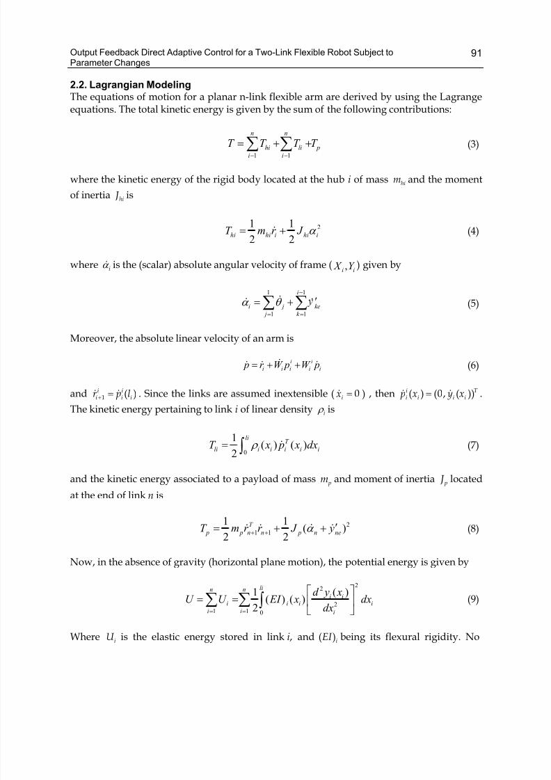
Output Feedback Direct Adaptive Control for a Two-Link Flexible Robot Subject toParameter Changes
91
2.2. Lagrangian ModelingThe equations of motion for a planar n-link flexible arm are derived by using the Lagrangeequations. The total kinetic energy is given by the sum of the following contributions:
1 1
n n
hi li p
i i
T T T T − −
= + +∑ ∑ (3)
where the kinetic energy of the rigid body located at the hub i of mass him and the moment
of inertia hi J is
21 1
2 2hi hi i hi iT m r J α = +& (4)
where iα & is the (scalar) absolute angular velocity of frame ( ,i i X Y ) given by
1 1
1 1
i
i j ke
j k
α θ −
= =
′= +∑ ∑&& & (5)
Moreover, the absolute linear velocity of an arm is
i i
i i i i i p r W p W p= + +&& & & (6)
and 1 ( )i ii i ir p l+ =& & . Since the links are assumed inextensible ( 0ix =& ) , then ( ) (0, ( ))i T
i i i i p x y x=& & .
The kinetic energy pertaining to link i of linear density i ρ is
0
1( ) ( )
2
liT
li i i i i iT x p x dx ρ = ∫ & (7)
and the kinetic energy associated to a payload of mass pm and moment of inertia p J located
at the end of link n is
2
1 1
1 1( )
2 2
T
p p n n p n neT m r r J yα + +′= + +&& & & (8)
Now, in the absence of gravity (horizontal plane motion), the potential energy is given by
22
21 1 0
( )1( ) ( )
2
lin ni i
i i i i
i i i
d y xU U EI x dx
dx= =
⎡ ⎤= = ⎢ ⎥
⎣ ⎦∑ ∑ ∫ (9)
Where iU is the elastic energy stored in link i, and ( )iEI being its flexural rigidity. No
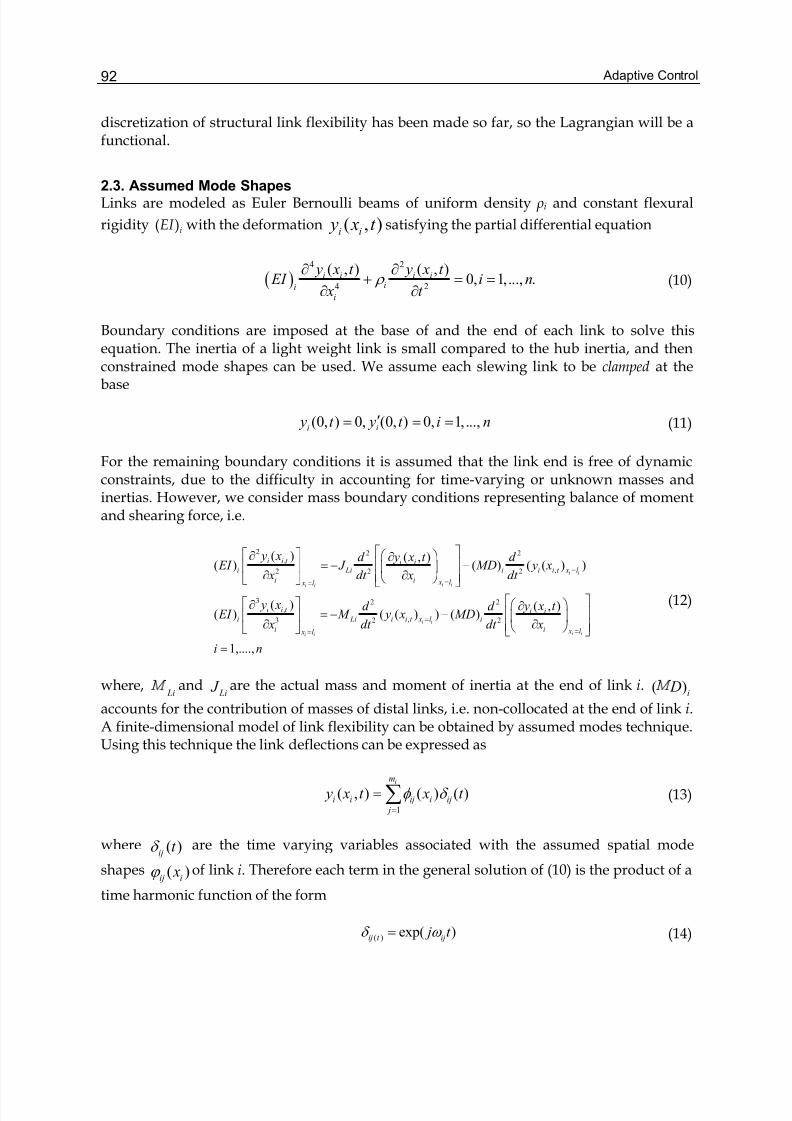
Adaptive Control92
discretization of structural link flexibility has been made so far, so the Lagrangian will be afunctional.
2.3. Assumed Mode ShapesLinks are modeled as Euler Bernoulli beams of uniform density ρi and constant flexural
rigidity ( )iEI with the deformation ( , )i i y x t satisfying the partial differential equation
( )4 2
4 2
( , ) ( , )0, 1,..., .i i i i
iii
y x t y x t EI i n
x t ρ
∂ ∂+ = =
∂ ∂ (10)
Boundary conditions are imposed at the base of and the end of each link to solve thisequation. The inertia of a light weight link is small compared to the hub inertia, and thenconstrained mode shapes can be used. We assume each slewing link to be clamped at thebase
(0, ) 0, (0, ) 0, 1, ...,i i y t y t i n′= = = (11)
For the remaining boundary conditions it is assumed that the link end is free of dynamicconstraints, due to the difficulty in accounting for time-varying or unknown masses andinertias. However, we consider mass boundary conditions representing balance of momentand shearing force, i.e.
2 2 2,
,2 2 2
3 2 2,
,3 2 2
( ) ( , )( ) ( ) ( ( ) )
( ) ( , )( ) ( ( ) ) ( )
1,..
i i
i ii i
i i
i ii i
i i t i ii Li i i i t x l
i i x l x l
i i t i ii Li i i t x l i
i i x l x l
y x y x t d d EI J MD y x
x dt x dt
y x y x t d d EI M y x MD
x dt dt x
i
=
==
=
==
⎡ ⎤⎡ ⎤∂ ⎛ ⎞∂⎢ ⎥= − −⎢ ⎥ ⎜ ⎟
∂ ∂⎢ ⎥⎝ ⎠⎣ ⎦ ⎣ ⎦
⎡ ⎤⎡ ⎤∂ ⎛ ⎞∂⎢ ⎥= − −⎢ ⎥ ⎜ ⎟
∂ ∂⎢ ⎥⎝ ⎠⎣ ⎦ ⎣ ⎦
= ..,n
(12)
where, Li
and Li J are the actual mass and moment of inertia at the end of link i. ( )i D
accounts for the contribution of masses of distal links, i.e. non-collocated at the end of link i.A finite-dimensional model of link flexibility can be obtained by assumed modes technique.Using this technique the link deflections can be expressed as
1
( , ) ( ) ( )im
i i ij i ij
j
y x t x t φ δ =
= ∑ (13)
where ( )ij t δ are the time varying variables associated with the assumed spatial mode
shapes ( )ij i xϕ of link i. Therefore each term in the general solution of (10) is the product of a
time harmonic function of the form
( ) exp( )ij t ij j t δ ω = (14)
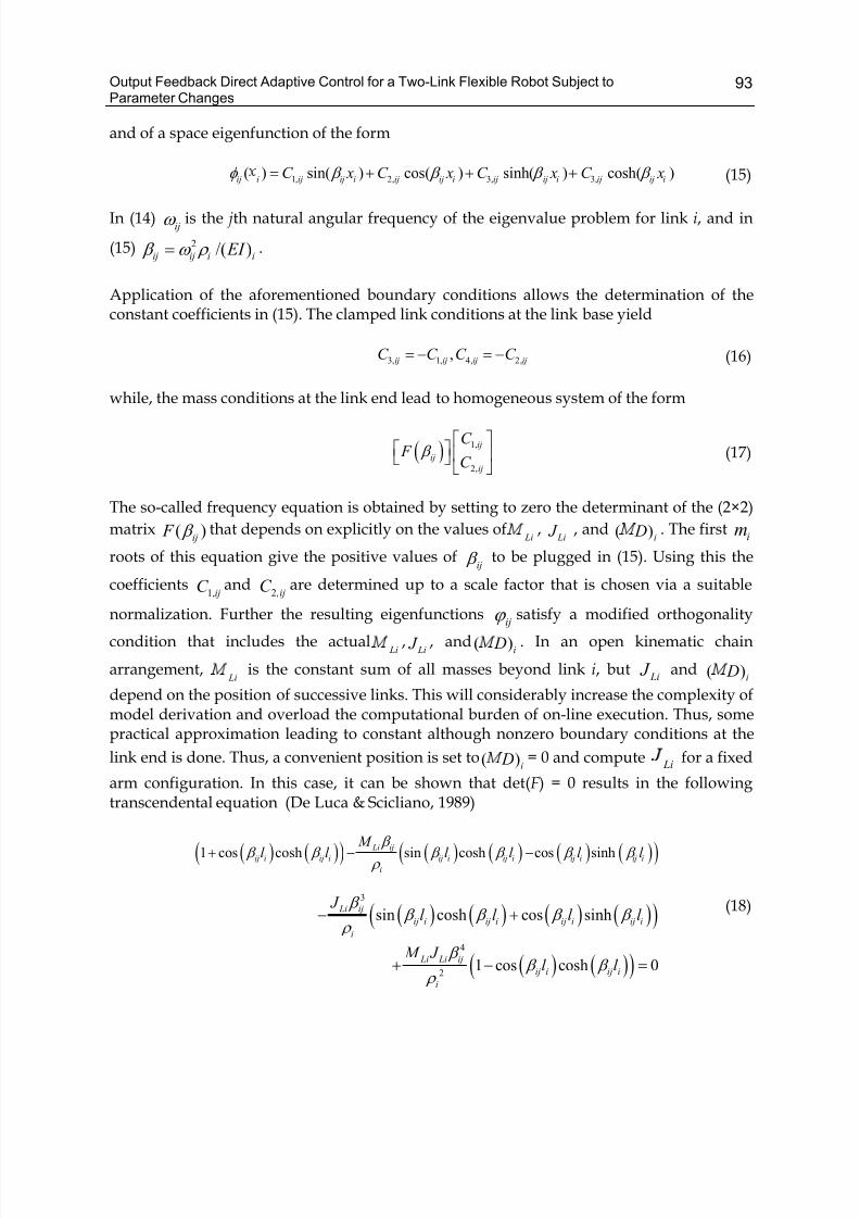
Output Feedback Direct Adaptive Control for a Two-Link Flexible Robot Subject toParameter Changes
93
and of a space eigenfunction of the form
1, 2, 3, 3,( ) sin( ) cos( ) sinh( ) cosh( )ij i ij ij i ij ij i ij ij i ij ij iC x C x C x C xφ β β β β = + + + (15)
In (14)ijω is the jth natural angular frequency of the eigenvalue problem for link i, and in
(15) 2 /( ) β ω ρ =ij ij i i EI .
Application of the aforementioned boundary conditions allows the determination of theconstant coefficients in (15). The clamped link conditions at the link base yield
3, 1, 4, 2,,ij ij ij ijC C C C = − = − (16)
while, the mass conditions at the link end lead to homogeneous system of the form
( ) 1,
2,
ij
ij
ij
C F
C β
⎡ ⎤⎡ ⎤ ⎢ ⎥⎣ ⎦
⎣ ⎦
(17)
The so-called frequency equation is obtained by setting to zero the determinant of the (2×2)
matrix ( )ij F β that depends on explicitly on the values of Li
, Li J , and ( )i D . The first
im
roots of this equation give the positive values ofij β to be plugged in (15). Using this the
coefficients1,ijC and
2,ijC are determined up to a scale factor that is chosen via a suitable
normalization. Further the resulting eigenfunctionsijϕ satisfy a modified orthogonality
condition that includes the actual Li
, Li J , and ( )i D . In an open kinematic chain
arrangement, Li
is the constant sum of all masses beyond link i, but Li J and ( )i D
depend on the position of successive links. This will considerably increase the complexity ofmodel derivation and overload the computational burden of on-line execution. Thus, somepractical approximation leading to constant although nonzero boundary conditions at the
link end is done. Thus, a convenient position is set to( )i D = 0 and compute Li
for a fixed
arm configuration. In this case, it can be shown that det(F ) = 0 results in the followingtranscendental equation (De Luca & Scicliano, 1989)
( ) ( )( ) ( ) ( ) ( ) ( )( )1 cos cosh sin cosh cos sinh Li ij
ij i ij i ij i ij i ij i ij i
i
M l l l l l l
β β β β β β β
ρ + − −
( ) ( ) ( ) ( )( )3
sin cosh cos sinh Li ij
ij i ij i ij i ij i
i
J l l l l
β β β β β
ρ − + (18)
( ) ( )( )4
21 cos cosh 0
Li Li ij
ij i ij i
i
M J l l
β β β
ρ + − =
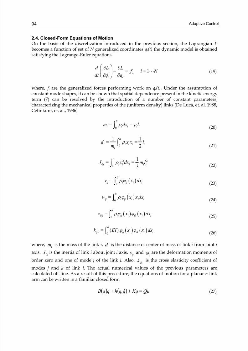
Adaptive Control94
2.4. Closed-Form Equations of MotionOn the basis of the discretization introduced in the previous section, the Lagrangian Lbecomes a function of set of N generalized coordinates qi(t) the dynamic model is obtainedsatisfying the Lagrange-Euler equations
, 1i
i i
d L L f i N
dt q q
⎛ ⎞∂ ∂− = =⎜ ⎟
∂ ∂⎝ ⎠L
& (19)
where, f i are the generalized forces performing work on qi(t). Under the assumption ofconstant mode shapes, it can be shown that spatial dependence present in the kinetic energyterm (7) can be resolved by the introduction of a number of constant parameters,characterizing the mechanical properties of the (uniform density) links (De Luca, et. al. 1988,Cetinkunt, et. al., 1986)
0
li
i i i i im = dx = ρ l ρ ∫ (20)
0
1 1
2
li
i i i i i
i
d = x x = l m
ρ ∫ (21)
2 2
00
1
3
li
i i i i i i J = x dx = m l ρ ∫ (22)
( )0
li
ij i ij i iv = φ x dx ρ ∫ (23)
( )0
li
ij i ij i i iw = φ x x dx ρ ∫ (24)
( ) ( )0
li
ijk i ij i ik i i z = φ x φ x dx ρ ∫
(25)
( ) ( )0
( )li
ijk i ij i ik i ik = EI φ x φ x dx∫
(26)
where,im is the mass of the link i, d is the distance of center of mass of link i from joint i
axis,0i J is the inertia of link i about joint i axis,
ijv andijω are the deformation moments of
order zero and one of mode j of the link i. Also,ijk k is the cross elasticity coefficient of
modes j and k of link i. The actual numerical values of the previous parameters arecalculated off-line. As a result of this procedure, the equations of motion for a planar n-linkarm can be written in a familiar closed form
( ) ( ) Qu= Kq+qq,h+qq B &&& (27)
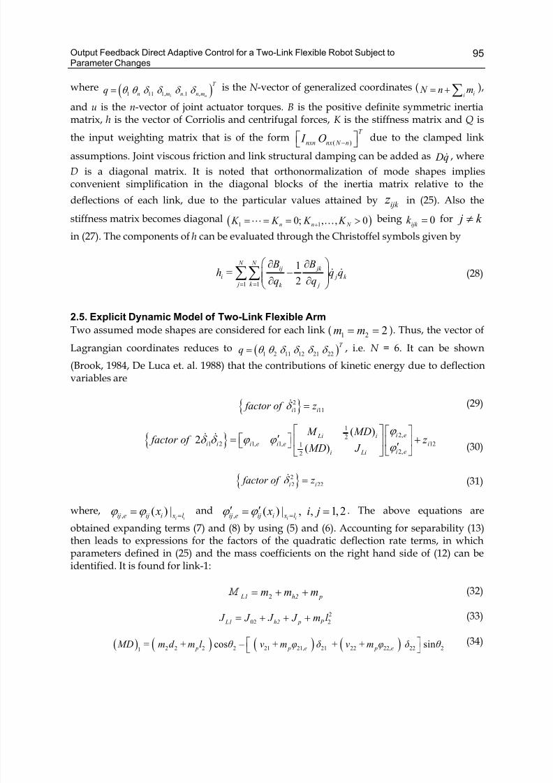
Output Feedback Direct Adaptive Control for a Two-Link Flexible Robot Subject toParameter Changes
95
where ( )11 11 1, ,1 , n
T
n m n n mq θ θ δ δ δ δ = is the N -vector of generalized coordinates (ii
N n m= +∑ ),
and u is the n-vector of joint actuator torques. B is the positive definite symmetric inertiamatrix, h is the vector of Corriolis and centrifugal forces, K is the stiffness matrix and Q is
the input weighting matrix that is of the form( )
T
nxn nx N n I O −⎡ ⎤⎣ ⎦ due to the clamped link
assumptions. Joint viscous friction and link structural damping can be added as Dq& , where
D is a diagonal matrix. It is noted that orthonormalization of mode shapes impliesconvenient simplification in the diagonal blocks of the inertia matrix relative to the
deflections of each link, due to the particular values attained byijk z in (25). Also the
stiffness matrix becomes diagonal ( )1 10; , , 0n n N K K K K += = = >L K being 0ijk
k = for j k ≠
in (27). The components of h can be evaluated through the Christoffel symbols given by
1 1
1
2
N N ij jk
i j k
j k k j
B Bh = q q
q q= =
⎛ ⎞∂ ∂−⎜ ⎟⎜ ⎟∂ ∂⎝ ⎠
∑∑ & & (28)
2.5. Explicit Dynamic Model of Two-Link Flexible Arm
Two assumed mode shapes are considered for each link (1 2 2m m= = ). Thus, the vector of
Lagrangian coordinates reduces to ( )1 2 11 12 21 22
T q θ θ δ δ δ δ = , i.e. N = 6. It can be shown
(Brook, 1984, De Luca et. al. 1988) that the contributions of kinetic energy due to deflectionvariables are
2
1 11i i factor of z δ =& (29)
1
2,21 2 1, 1, 121
2,2
( )2
( )
i e Li i
i i i e i e i
i ei Li
M MD factor of z
MD J
ϕ δ δ ϕ ϕ
ϕ
⎡ ⎤ ⎡ ⎤′⎡ ⎤= +⎢ ⎥ ⎢ ⎥⎣ ⎦ ′⎣ ⎦⎣ ⎦
& & (30)
2
2 22i i factor of z δ =& (31)
where,, ( ) |
i iij e ij i x l xϕ ϕ == and, ( ) | , , 1, 2
i iij e ij i x l x i jϕ ϕ =′ ′= = . The above equations are
obtained expanding terms (7) and (8) by using (5) and (6). Accounting for separability (13)then leads to expressions for the factors of the quadratic deflection rate terms, in whichparameters defined in (25) and the mass coefficients on the right hand side of (12) can beidentified. It is found for link-1:
2 L1 h2 pm m m= + + (32)
2
02 2 L1 h2 p P J J J J m l = + + + (33)
( ) ( ) ( ) ( )2 2 2 2 21 21, 21 22 22, 22 21cos sin p p e p e MD = m d + m l θ v + m φ δ + v + m φ δ θ ⎡ ⎤− ⎣ ⎦
(34)
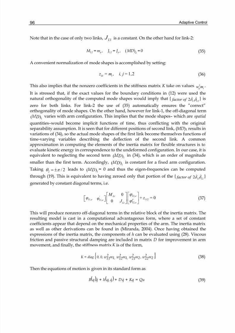
Adaptive Control96
Note that in the case of only two links, 1 L J is a constant. On the other hand for link-2:
( )20L2 p L2 p M = m , J = J , MD = (35)
A convenient normalization of mode shapes is accomplished by setting:
1,2iii i
z = m , i, j = (36)
This also implies that the nonzero coefficients in the stiffness matrix K take on values 2
ij iw m .
It is stressed that, if the exact values for the boundary conditions in (12) were used thenatural orthogonality of the computed mode shapes would imply that
11 122δ δ & & factor of is
zero for both links. For link-2 the use of (35) automatically ensures the ”correct”orthogonality of mode shapes. On the other hand, however for link-1, the off-diagonal term
1( ) D varies with arm configuration. This implies that the mode shapes– which are spatial
quantities–would become implicit functions of time, thus conflicting with the originalseparability assumption. It is seen that for different positions of second link, ( MD)1 results invariations of (34), so the actual mode shapes of the first link become themselves functions oftime-varying variables describing the deflection of the second link. A commonapproximation in computing the elements of the inertia matrix for flexible structures is toevaluate kinetic energy in correspondence to the undeformed configuration. In our case, it isequivalent to neglecting the second term
1( ) D in (34), which is an order of magnitude
smaller than the first term. Accordingly,1( ) D is constant for a fixed arm configuration.
Taking2 / 2θ π = ± leads to
1( ) D = 0 and thus the eigen-frequencies can be computed
through (19). This is equivalent to having zeroed only that portion of the 11 122δ δ & & factor of
generated by constant diagonal terms, i.e.
12,
11, 11211,12,
00
0
e Li' e e
e Li
M φ + z =φ
J
ϕ
ϕ
⎡ ⎤⎡ ⎤⎡ ⎤ ⎢ ⎥⎢ ⎥⎣ ⎦ ′⎣ ⎦ ⎣ ⎦
(37)
This will produce nonzero off-diagonal terms in the relative block of the inertia matrix. Theresulting model is cast in a computational advantageous form, where a set of constantcoefficients appear that depend on the mechanical properties of the arm. The inertia matrixas well as other derivations can be found in (Miranda, 2004). Once having obtained theexpressions of the inertia matrix, the components of h can be evaluated using (28). Viscousfriction and passive structural damping are included in matrix D for improvement in armmovement, and finally, the stiffness matrix K is of the form,
2m222w ,2m2
21w1,m212w1,m2
11w0,0,diag=K (38)
Then the equations of motion is given in its standard form as
Qu=Kq+qD+qq,h+qqB &&&& (39)
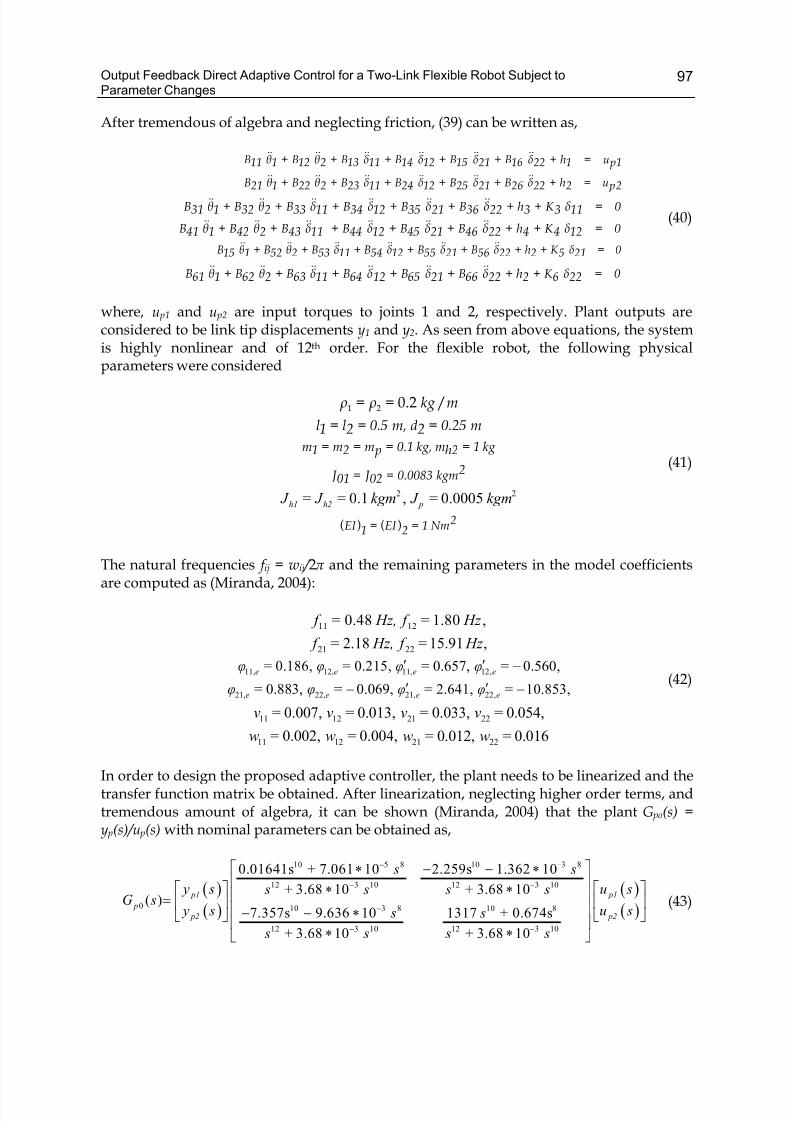
Output Feedback Direct Adaptive Control for a Two-Link Flexible Robot Subject toParameter Changes
97
After tremendous of algebra and neglecting friction, (39) can be written as,
1 pu1h22δ 16B21δ 15B12δ 14B11δ 13B2θ12B1θ11B =++++++ &&&&&&&&&&&&
2 pu2h22δ 26B21δ 25B12δ 24B11δ 23B2θ22B1θ21B =++++++ &&&&&&&&&&&&
011δ 3K 3h22δ 36B21δ 35B12δ 34B11δ 33B2θ32B1θ31B =+++++++ &&&&&&&&&&&&
012δ 4K 4h22δ 46B21δ 45B12δ 44B11δ 43B2θ42B1θ41B =+++++++ &&&&&&&&&&&& (40)
021δ 5K 2h22δ 56B21δ 55B12δ 54B11δ 53B2θ52B1θ15B =+++++++ &&&&&&&&&&&&
022δ 6K 2h22δ 66B21δ 65B12δ 64B11δ 63B2θ62B1θ61B =+++++++ &&&&&&&&&&&&
where, u p1 and u p2 are input torques to joints 1 and 2, respectively. Plant outputs areconsidered to be link tip displacements y1 and y2. As seen from above equations, the systemis highly nonlinear and of 12th order. For the flexible robot, the following physicalparameters were considered
1 2 0.2 / ρ = ρ = kg m
m0.25=2dm,0.5=2l=1l
kg1=h2mkg,0.1= pm=2m=1m
2kgm0.0083=02 J =01 J (41)
2 20.1 , 0.0005h1 h2 p J = J = kgm J = kgm
( ) ( ) 2Nm1=2EI =1EI
The natural frequencies f ij = wij / 2 π and the remaining parameters in the model coefficientsare computed as (Miranda, 2004):
11 120.48 1.80 , f = Hz, f = Hz
21 222.18 15.91 , f = Hz, f = Hz
11, 12,0.186, 0.215,e eφ = φ = 11, 12,0.657, 0.560,e eφ = φ =′ ′ −
21, 22,0.883, 0.069,e eφ = φ = − 21, 22,2.641, 10.853,e eφ = φ =′ ′ − (42)
11 120.007, 0.013,v = v = 21 220.033, 0.054,v = v =
11 120.002, 0.004,w = w =
21 220.012, 0.016w = w =
In order to design the proposed adaptive controller, the plant needs to be linearized and thetransfer function matrix be obtained. After linearization, neglecting higher order terms, andtremendous amount of algebra, it can be shown (Miranda, 2004) that the plant G po(s) =y p(s)/u p(s) with nominal parameters can be obtained as,
( )
( )
( )
( )
10 5 8 10 3 8
12 3 10 12 3 10
0 10 3 8 10 8
12 3 10 12 3 10
0.01641s 7.061 10 2.259s 1.362 10
3.68 10 3.68 10( )
7.357s 9.636 10 1317 0.674s
3.68 10 3.68 10
p1 p1
p
p2 p2
+ s s
y s u s s + s s + sG s
y s u s s s +
s + s s + s
− −
− −
−
− −
⎡ ⎤∗ − − ∗⎢ ⎥⎡ ⎤ ⎡ ⎤∗ ∗⎢ ⎥= ⎢ ⎥ ⎢ ⎥⎢ ⎥− − ∗⎣ ⎦ ⎣ ⎦⎢ ⎥
∗ ∗⎣ ⎦
(43)
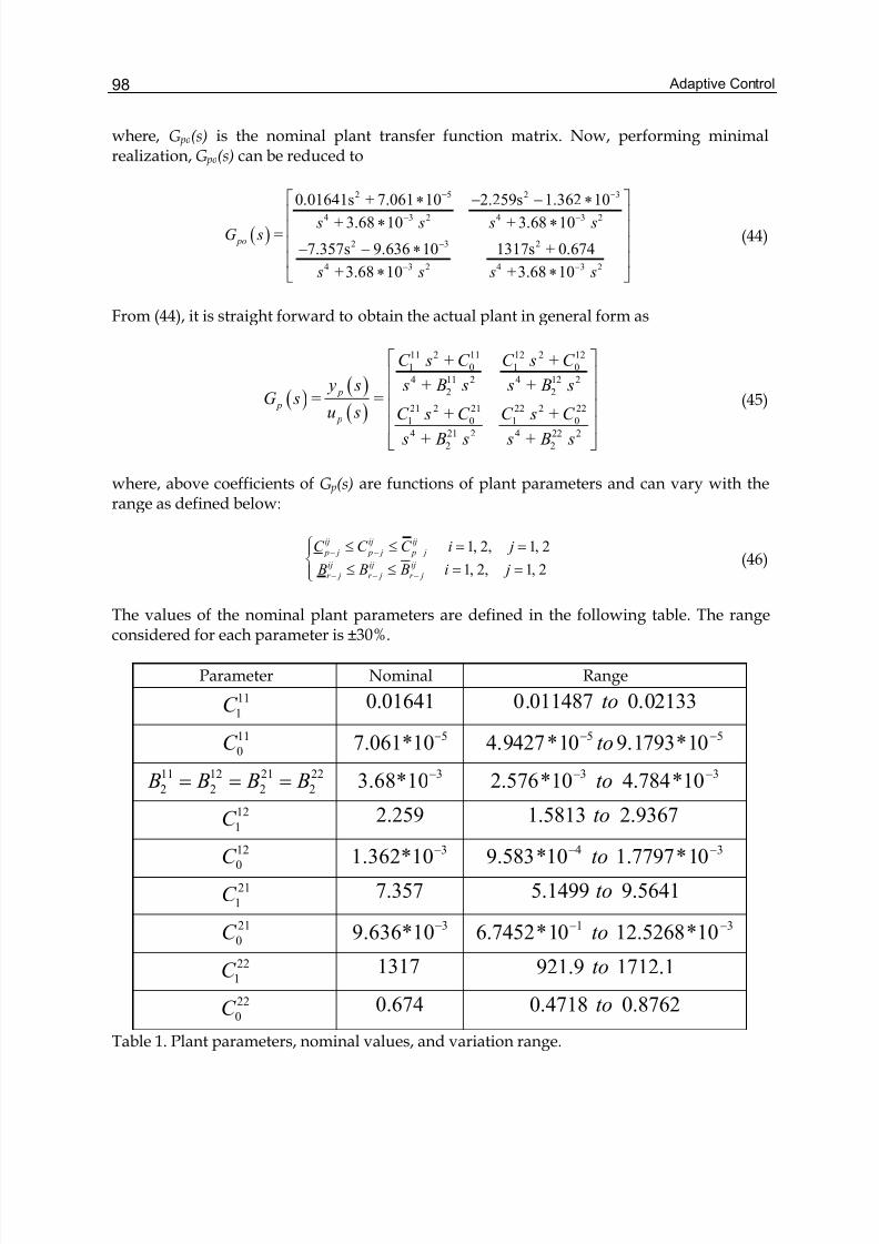
Adaptive Control98
where, G po(s) is the nominal plant transfer function matrix. Now, performing minimalrealization, G po(s) can be reduced to
( )
2 5 2 3
4 3 2 4 3 2
2 3 2
4 3 2 4 3 2
0.01641s 7.061 10 2.259s 1.362 10
3.68 10 3.68 10
7.357s 9.636 10 1317s 0.674
3.68 10 3.68 10
po
+
s + s s + sG s =
+
s + s s + s
− −
− −
−
− −
⎡ ⎤∗ − − ∗⎢ ⎥∗ ∗⎢ ⎥⎢ ⎥− − ∗⎢ ⎥
∗ ∗⎣ ⎦
(44)
From (44), it is straight forward to obtain the actual plant in general form as
( )( )
( )
11 2 11 12 2 12
1 0 1 0
4 11 2 4 12 2
2 2
21 2 21 22 2 22
1 0 1 0
4 21 2 4 22 2
2 2
p
p
p
C s + C C s + C
y s s + B s s + B sG s = =
u s C s + C C s + C
s + B s s + B s
⎡ ⎤⎢ ⎥⎢ ⎥⎢ ⎥⎢ ⎥⎣ ⎦
(45)
where, above coefficients of G p(s) are functions of plant parameters and can vary with therange as defined below:
1, 2, 1, 2
1, 2, 1, 2
ij ij ij
p j p j p j
ij ij ij
r j r j r j
C C C i j
B B B i j
− − −
− − −
⎧ ≤ ≤ = =⎪⎨
≤ ≤ = =⎪⎩
(46)
The values of the nominal plant parameters are defined in the following table. The rangeconsidered for each parameter is ±30%.
Parameter Nominal Range
11
1C 0.01641 0.011487 0.02133to
11
0C 57.061*10−
5 54.9427*10 9.1793*10to− −
11 12 21 22
2 2 2 2 B B B B= = = 33.68*10−
3 32.576*10 4.784*10to− −
12
1C 2.259 1.5813 2.9367to
12
0C 31.362*10−
4 39.583*10 1.7797*10to− −
21
1C 7.357 5.1499 9.5641to
21
0C 39.636*10−
1 36.7452*10 12.5268*10to− −
22
1C 1317 921.9 1712.1to
22
0C 0.674 0.4718 0.8762to
Table 1. Plant parameters, nominal values, and variation range.
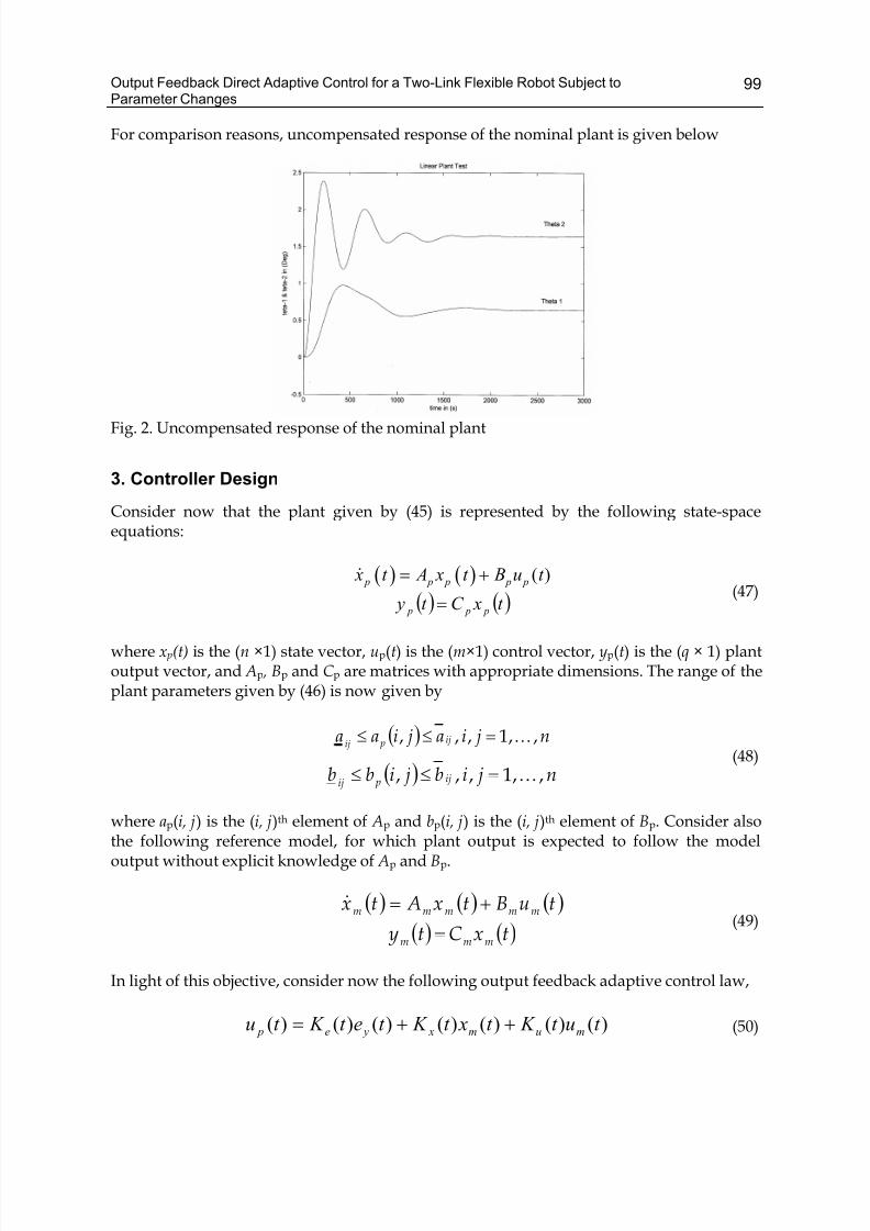
Output Feedback Direct Adaptive Control for a Two-Link Flexible Robot Subject toParameter Changes
99
For comparison reasons, uncompensated response of the nominal plant is given below
Fig. 2. Uncompensated response of the nominal plant
3. Controller Design
Consider now that the plant given by (45) is represented by the following state-spaceequations:
( ) ( ) ( ) p p p p p x t A x t B u t = +&
( ) ( )t xC t y p p p = (47)
where x p(t) is the (n ×1) state vector, up(t) is the (m×1) control vector, yp(t) is the (q × 1) plantoutput vector, and Ap , Bp and C p are matrices with appropriate dimensions. The range of theplant parameters given by (46) is now given by
( ) n jia jiaa ij pij,,1,,, K=≤≤
( ) n jib jibb ij pij,,1,,, K=≤≤
(48)
where ap(i, j) is the (i, j)th element of Ap and bp(i, j) is the (i, j)th element of Bp. Consider alsothe following reference model, for which plant output is expected to follow the modeloutput without explicit knowledge of Ap and Bp.
( ) ( ) ( )tuBtx Atx mmmmm +=&
( ) ( )txC ty mmm = (49)
In light of this objective, consider now the following output feedback adaptive control law,
)()()()()()()( t ut K t xt K t et K t u mum x ye p ++= (50)
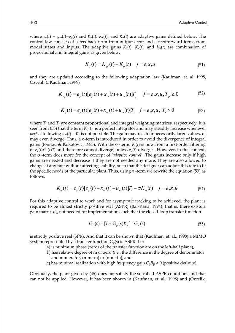
Adaptive Control100
where ey(t) = ym(t)−yp(t) and K e(t), K x(t), and K u(t) are adaptive gains defined below. Thecontrol law consists of a feedback term from output error and a feedforward terms frommodel states and inputs. The adaptive gains K e(t), K x(t), and K u(t) are combination ofproportional and integral gains as given below,
( ) ( ) ( ) , , j pj ij K t K t K t j e x u= + = (51)
and they are updated according to the following adaptation law (Kaufman, et. al. 1998,Ozcelik & Kaufman, 1999)
( ) ( )[ ( ) ( ) ( )] , , , 0 pj y y m m p p K t e t e t x t u t T j e x u T = + + = ≥ (52)
( ) ( )[ ( ) ( ) ( )] , , , 0ij y y m m i i K t e t e t x t u t T j e x u T = + + = > (53)
where T i and T p are constant proportional and integral weighting matrices, respectively. It isseen from (53) that the term K ij(t) is a perfect integrator and may steadily increase whenever perfect following (ey(t) = 0) is not possible. The gain may reach unnecessarily large values, ormay even diverge. Thus, a σ-term is introduced in order to avoid the divergence of integralgains (Ionnou & Kokotovic, 1983). With the σ -term, K i(t) is now from a first-order filteringof ey(t)r T (t)T i and therefore cannot diverge, unless ey(t) diverges. However, in this context,the σ -term does more for the concept of ‘adaptive control’. The gains increase only if highgains are needed and decrease if they are not needed any more. They are also allowed tochange at any rate without affecting stability, such that the designer can adjust this rate to fitthe specific needs of the particular plant. Thus, using σ -term we rewrite the equation (53) asfollows,
( ) ( )[ ( ) ( ) ( )] ( ) , ,ij y y m m i ij
K t e t e t x t u t T K t j e x uσ = + + − = (54)
For this adaptive control to work and for asymptotic tracking to be achieved, the plant isrequired to be almost strictly positive real (ASPR) (Bar-Kana, 1994); that is, there exists again matrix K e, not needed for implementation, such that the closed-loop transfer function
)(])([)( 1 sGK sGI sG pe pc−+= (55)
is strictly positive real (SPR). And that it can be shown that (Kaufman, et. al., 1998) a MIMOsystem represented by a transfer function Gp(s) is ASPR if it:
a) is minimum phase (zeros of the transfer function are on the left-half plane),b) has relative degree of m or zero (i.e., the difference in the degree of denominator
and numerator, (n-m=m) or (n-m=0)), andc) has minimal realization with high frequency gain C pBp > 0 (positive definite).
Obviously, the plant given by (45) does not satisfy the so-called ASPR conditions and thatcan not be applied. However, it has been shown in (Kaufman, et. al., 1998) and (Ozcelik,
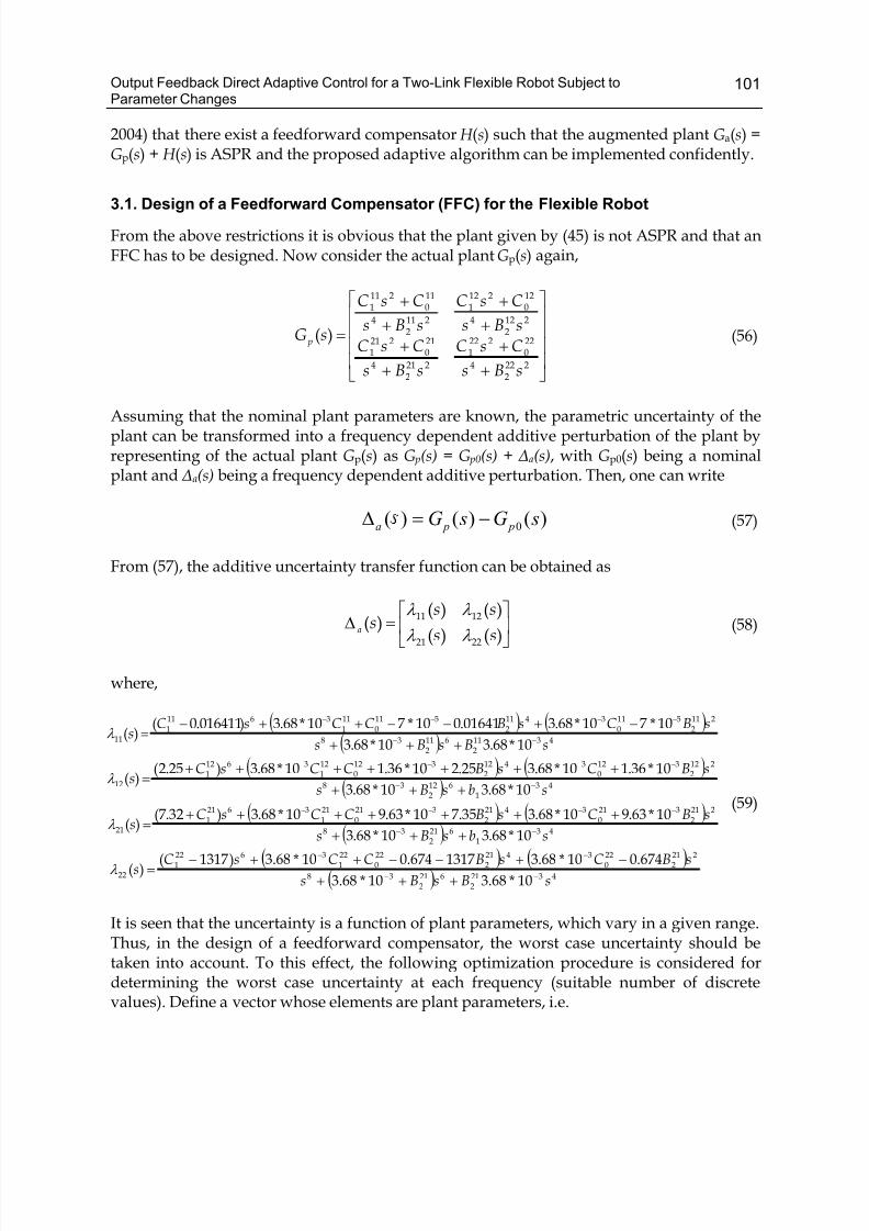
Output Feedback Direct Adaptive Control for a Two-Link Flexible Robot Subject toParameter Changes
101
2004) that there exist a feedforward compensator H (s) such that the augmented plant Ga(s) =Gp(s) + H (s) is ASPR and the proposed adaptive algorithm can be implemented confidently.
3.1. Design of a Feedforward Compensator (FFC) for the Flexible Robot
From the above restrictions it is obvious that the plant given by (45) is not ASPR and that anFFC has to be designed. Now consider the actual plant Gp(s) again,
⎥⎥⎥⎥
⎦
⎤
⎢⎢⎢⎢
⎣
⎡
+
+
+
++
+
+
+
=
2222
4
220
2221
2212
4
210
2211
2122
4
120
2121
2112
4
110
2111
)(
sBs
C sC
sBs
C sC sBs
C sC
sBs
C sC
sG p (56)
Assuming that the nominal plant parameters are known, the parametric uncertainty of theplant can be transformed into a frequency dependent additive perturbation of the plant byrepresenting of the actual plant Gp(s) as G p(s) = G p0(s) + Δa(s), with Gp0(s) being a nominalplant and Δa(s) being a frequency dependent additive perturbation. Then, one can write
0( ) ( ) ( )a p pG s G sΔ = − (57)
From (57), the additive uncertainty transfer function can be obtained as
⎥⎦
⎤⎢⎣
⎡=Δ
)()(
)()()(
2221
1211
ss
sssa
λ λ
λ λ (58)
where,
( ) ( )( ) 4311
2611
238
2112
5110
34112
5110
111
36111
1110*68.310*68.3
10*710*68.301641.010*710*68.3)016411.0()(
sBsBs
sBC sBC C sC s
−−
−−−−
+++
−+−−++−=λ
( ) ( )( ) 43
1612
238
2122
3120
34122
3120
121
36121
1210*68.310*68.3
10*36.110*68.325.210*36.110*68.3)25.2()(
sbsBs
sBC sBC C sC s
−−
−−−−
+++
+++++++=λ
( ) ( )
( ) 431
6212
38
2212
3210
34212
3210
211
36211
2110*68.310*68.3
10*63.910*68.335.710*63.910*68.3)32.7()(
sbsBs
sBC sBC C sC s
−−
−−−−
+++
+++++++=λ
(59)
( ) ( )( ) 4321
2621
238
2212
220
34212
220
221
36221
2210*68.310*68.3
674.010*68.31317674.010*68.3)1317()(
sBsBs
sBC sBC C sC s
−−
−−
+++
−+−−++−=λ
It is seen that the uncertainty is a function of plant parameters, which vary in a given range.Thus, in the design of a feedforward compensator, the worst case uncertainty should betaken into account. To this effect, the following optimization procedure is considered fordetermining the worst case uncertainty at each frequency (suitable number of discretevalues). Define a vector whose elements are plant parameters, i.e.
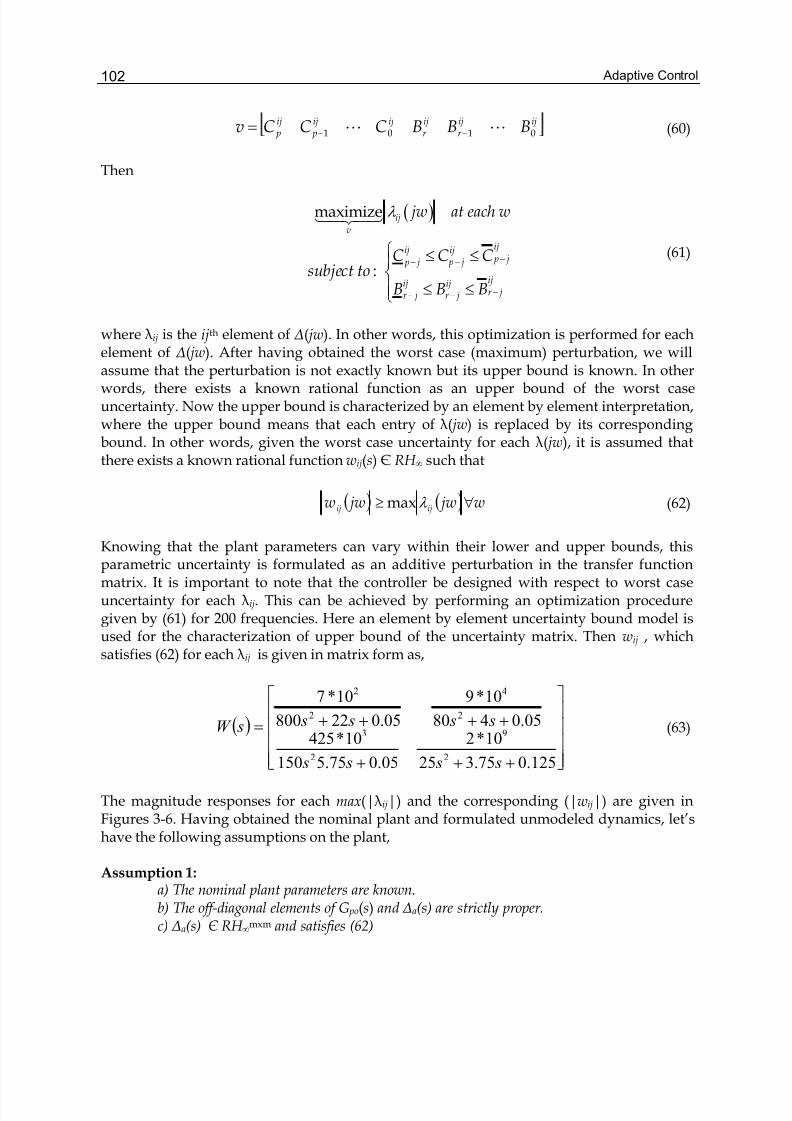
Adaptive Control102
ijijr
ijr
ijij p
ij p BBBC C C v 0101 LL −−= (60)
Then
( )λ 14243maximize ij
v
jw at each w
−−−
−−−
⎧ ≤ ≤⎪⎨⎪ ≤ ≤⎩
:
ijij ij p j p j p j
ijij ijr jr jr j
C C C subject to
B B B
(61)
where λij is the ijth element of Δ( jw). In other words, this optimization is performed for eachelement of Δ( jw). After having obtained the worst case (maximum) perturbation, we willassume that the perturbation is not exactly known but its upper bound is known. In otherwords, there exists a known rational function as an upper bound of the worst caseuncertainty. Now the upper bound is characterized by an element by element interpretation,where the upper bound means that each entry of λ( jw) is replaced by its correspondingbound. In other words, given the worst case uncertainty for each λ( jw), it is assumed thatthere exists a known rational function wij(s) Є RH ∞ such that
( ) ( ) w jw jww ijij ∀≥ λ max (62)
Knowing that the plant parameters can vary within their lower and upper bounds, thisparametric uncertainty is formulated as an additive perturbation in the transfer functionmatrix. It is important to note that the controller be designed with respect to worst caseuncertainty for each λij. This can be achieved by performing an optimization proceduregiven by (61) for 200 frequencies. Here an element by element uncertainty bound model isused for the characterization of upper bound of the uncertainty matrix. Then wij , whichsatisfies (62) for each λij is given in matrix form as,
( )
⎥⎥⎥⎥
⎦
⎤
⎢⎢⎢⎢
⎣
⎡
+++
++++=
125.075.325
10*2
05.075.5150
10*42505.0480
10*9
05.022800
10*7
2
9
2
3
2
4
2
2
s s s s
s s s s sW (63)
The magnitude responses for each max(| λij|) and the corresponding (|wij|) are given inFigures 3-6. Having obtained the nominal plant and formulated unmodeled dynamics, let’shave the following assumptions on the plant,
Assumption 1:a) The nominal plant parameters are known.b) The off-diagonal elements of G po(s) and Δa(s) are strictly proper.c) Δa(s) Є RH ∞mxm and satisfies (62)
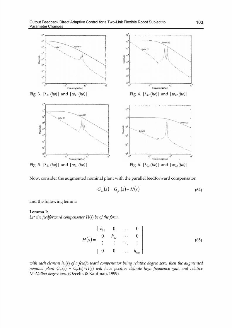
Output Feedback Direct Adaptive Control for a Two-Link Flexible Robot Subject toParameter Changes
103
Fig. 3. | λ11 ( jw)| and |w11 (jw)| Fig. 4. | λ12 ( jw)| and |w12 (jw)|
Fig. 5. | λ21 ( jw)| and |w21 (jw)| Fig. 6. | λ22 ( jw)| and |w22 (jw)|
Now, consider the augmented nominal plant with the parallel feedforward compensator
( ) ( ) ( ) s H sG sG poao += (64)
and the following lemma
Lemma 1:
Let the feedforward compensator H (s) be of the form,
( )
⎥⎥⎥⎥
⎦
⎤
⎢⎢⎢⎢
⎣
⎡
=
mmh
h
h
s H
K
MOMM
L
K
00
00
00
22
11
(65)
with each element hii(s) of a feedforward compensator being relative degree zero, then the augmentednominal plant Gao(s) = G po(s)+H (s) will have positive definite high frequency gain and relative McMillan degree zero (Ozcelik & Kaufman, 1999).
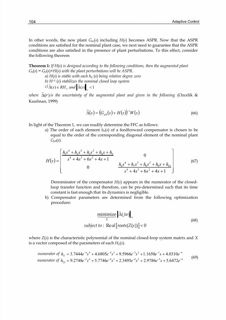
Adaptive Control104
In other words, the new plant Gao(s) including H (s) becomes ASPR. Now that the ASPRconditions are satisfied for the nominal plant case, we next need to guarantee that the ASPRconditions are also satisfied in the presence of plant perturbations. To this effect, considerthe following theorem
Theorem 1: If H (s) is designed according to the following conditions, then the augmented plantGa(s) = G p(s)+H (s) with the plant perturbations will be ASPR.
a) H (s) is stable with each hij (s) being relative degree zero b) H −1 (s) stabilizes the nominal closed loop systemc) ( ) ( ) 1 s RH and s∞ ∞Δ ∈ Δ <% %
where ( )Δ% is the uncertainty of the augmented plant and given in the following (Ozcelik &
Kaufman, 1999)
( ) ( ) ( )( ) ( ) sW s H sG s p
1
0
~ −+=Δ (66)
In light of the Theorem 1, we can readily determine the FFC as follows:a) The order of each element hii(s) of a feedforward compensator is chosen to be
equal to the order of the corresponding diagonal element of the nominal plantG p0(s).
( )
⎥⎥⎥⎥
⎦
⎤
⎢⎢⎢⎢
⎣
⎡
++++
++++++++
++++
=
14640
01464
234
109
2
8
3
7
4
6
234
54
2
3
3
2
4
1
s s s s
h sh sh sh sh s s s s
h sh sh sh sh
s H (67)
Denominator of the compensator H (s) appears in the numerator of the closed-loop transfer function and therefore, can be pre-determined such that its timeconstant is fast enough that its dynamics is negligible.
b) Compensator parameters are determined from the following optimizationprocedure:
∞Δ%14243minimize ( )
X
jw
[ ] <: Re ( ( )) 0subject to al roots Z s
(68)
where Z(s) is the characteristic polynomial of the nominal closed-loop system matrix and X is a vector composed of the parameters of each H ij(s).
numerator of 43233444
11 0310.41650.15966.96805.47444.3 −−−−− ++++= e se se se seh
numerator of 45243445
22 6472.59786.23495.27746.52748.9 −−−−− ++++= e se se se seh (69)
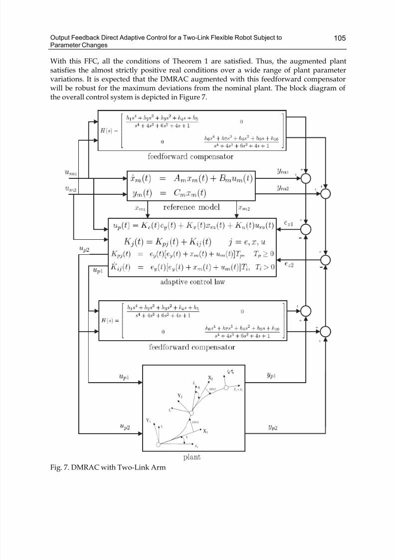
Output Feedback Direct Adaptive Control for a Two-Link Flexible Robot Subject toParameter Changes
105
With this FFC, all the conditions of Theorem 1 are satisfied. Thus, the augmented plantsatisfies the almost strictly positive real conditions over a wide range of plant parametervariations. It is expected that the DMRAC augmented with this feedforward compensatorwill be robust for the maximum deviations from the nominal plant. The block diagram ofthe overall control system is depicted in Figure 7.
Fig. 7. DMRAC with Two-Link Arm
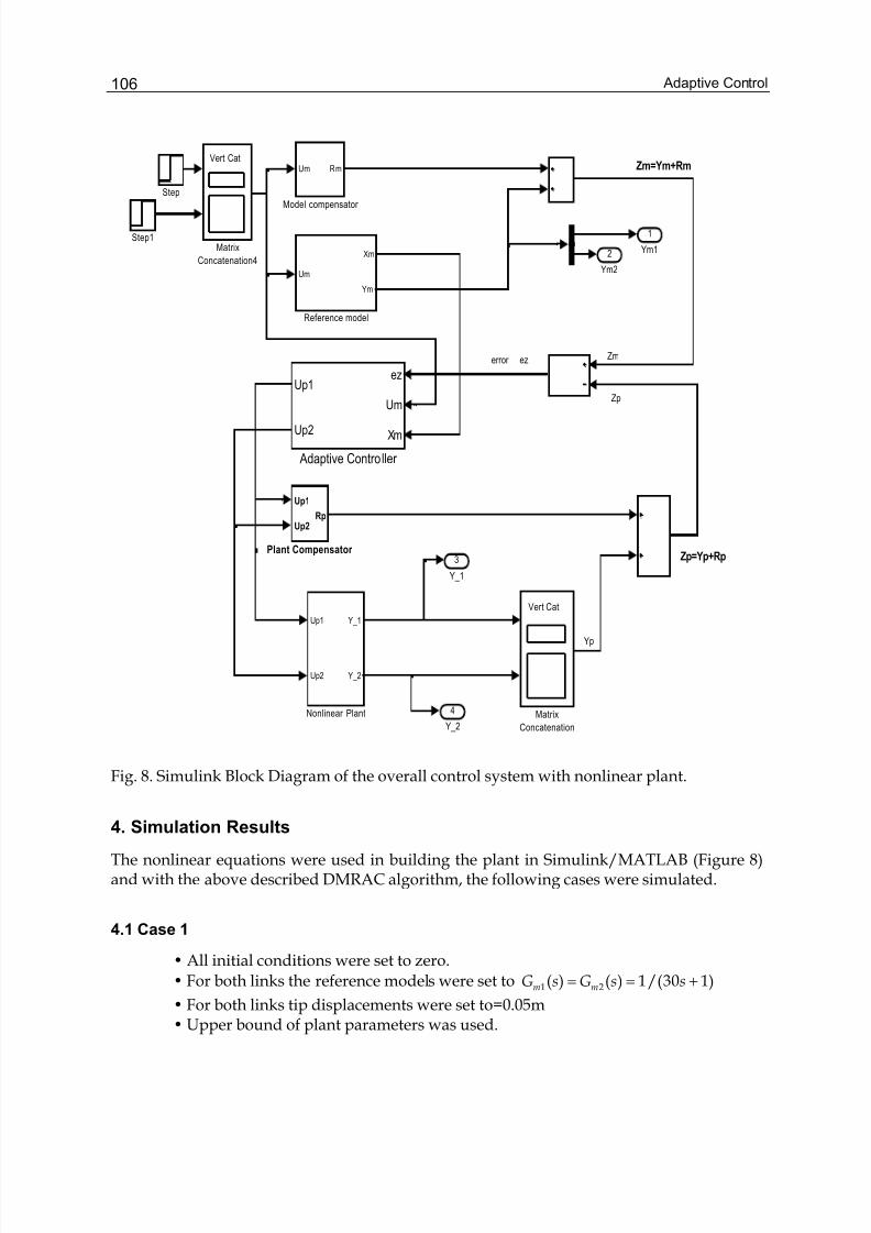
Adaptive Control106
Yp
Zp=Yp+Rp
Zm=Ym+Rm
Zm
Zp
ezerror
4
Y_2
3
Y_1
2
Ym2
1
Ym1
Step1
Step
Um
Xm
Ym
Reference model
Up1
Up2Rp
Plant Compensator
Up1
Up2
Y_1
Y_2
Nonlinear Plant
Um Rm
Model compensator
Vert Cat
Matrix
Concatenation4
Vert Cat
Matrix
Concatenation
m
ez
Um
Xm
Up1
Up2
Adaptive Controller
Fig. 8. Simulink Block Diagram of the overall control system with nonlinear plant.
4. Simulation Results
The nonlinear equations were used in building the plant in Simulink/MATLAB (Figure 8)and with the above described DMRAC algorithm, the following cases were simulated.
4.1 Case 1
• All initial conditions were set to zero.
• For both links the reference models were set to = = +1 2( ) ( ) 1/(30 1)m mG s G s s
• For both links tip displacements were set to=0.05m• Upper bound of plant parameters was used.
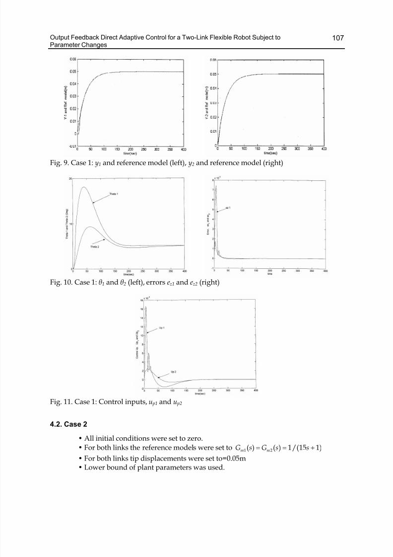
Output Feedback Direct Adaptive Control for a Two-Link Flexible Robot Subject toParameter Changes
107
Fig. 9. Case 1: y1 and reference model (left), y2 and reference model (right)
Fig. 10. Case 1: θ1 and θ2 (left), errors ez1 and ez2 (right)
Fig. 11. Case 1: Control inputs, u p1 and u p2
4.2. Case 2
• All initial conditions were set to zero.
• For both links the reference models were set to = = +1 2( ) ( ) 1/(15 1)m mG s G s s
• For both links tip displacements were set to=0.05m• Lower bound of plant parameters was used.
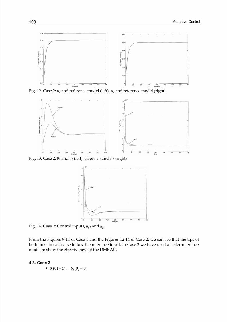
Adaptive Control108
Fig. 12. Case 2: y1 and reference model (left), y2 and reference model (right)
Fig. 13. Case 2: θ1 and θ2 (left), errors ez1 and ez2 (right)
Fig. 14. Case 2: Control inputs, u p1 and u p2
From the Figures 9-11 of Case 1 and the Figures 12-14 of Case 2, we can see that the tips ofboth links in each case follow the reference input. In Case 2 we have used a faster referencemodel to show the effectiveness of the DMRAC.
4.3. Case 3
• θ θ = =o o1 2(0) 5 , (0) 0
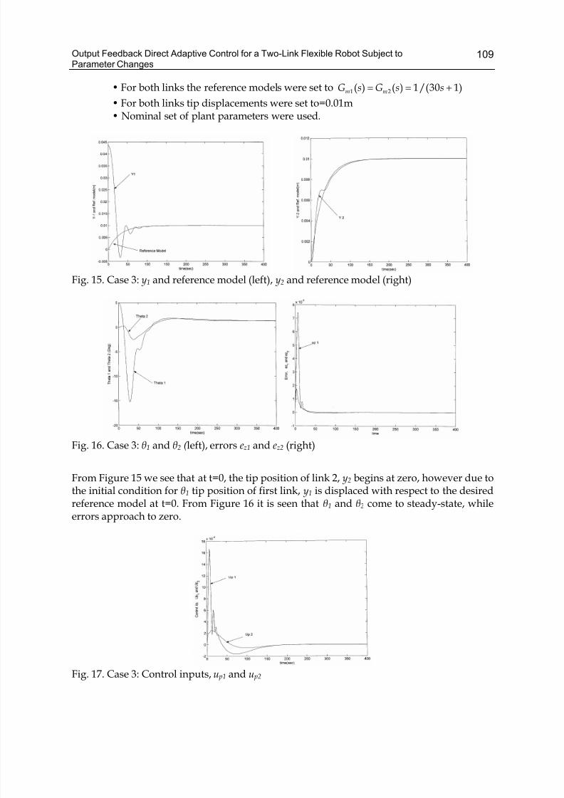
Output Feedback Direct Adaptive Control for a Two-Link Flexible Robot Subject toParameter Changes
109
• For both links the reference models were set to = = +1 2( ) ( ) 1/(30 1)m mG s G s s
• For both links tip displacements were set to=0.01m• Nominal set of plant parameters were used.
Fig. 15. Case 3: y1 and reference model (left), y2 and reference model (right)
Fig. 16. Case 3: θ1 and θ2 ( left), errors ez1 and ez2 (right)
From Figure 15 we see that at t=0, the tip position of link 2, y2 begins at zero, however due tothe initial condition for θ1 tip position of first link, y1 is displaced with respect to the desiredreference model at t=0. From Figure 16 it is seen that θ1 and θ2 come to steady-state, whileerrors approach to zero.
Fig. 17. Case 3: Control inputs, u p1 and u p2
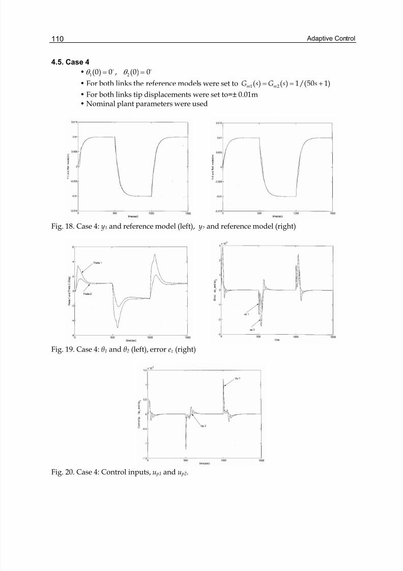
Adaptive Control110
4.5. Case 4
•θ θ = =o o1 2(0) 0 , (0) 0
• For both links the reference models were set to = = +1 2( ) ( ) 1/(50 1)m mG s G s s
• For both links tip displacements were set to=± 0.01m• Nominal plant parameters were used
Fig. 18. Case 4: y1 and reference model (left), y2 and reference model (right)
Fig. 19. Case 4: θ1 and θ2 (left), error ez (right)
Fig. 20. Case 4: Control inputs, u p1 and u p2.
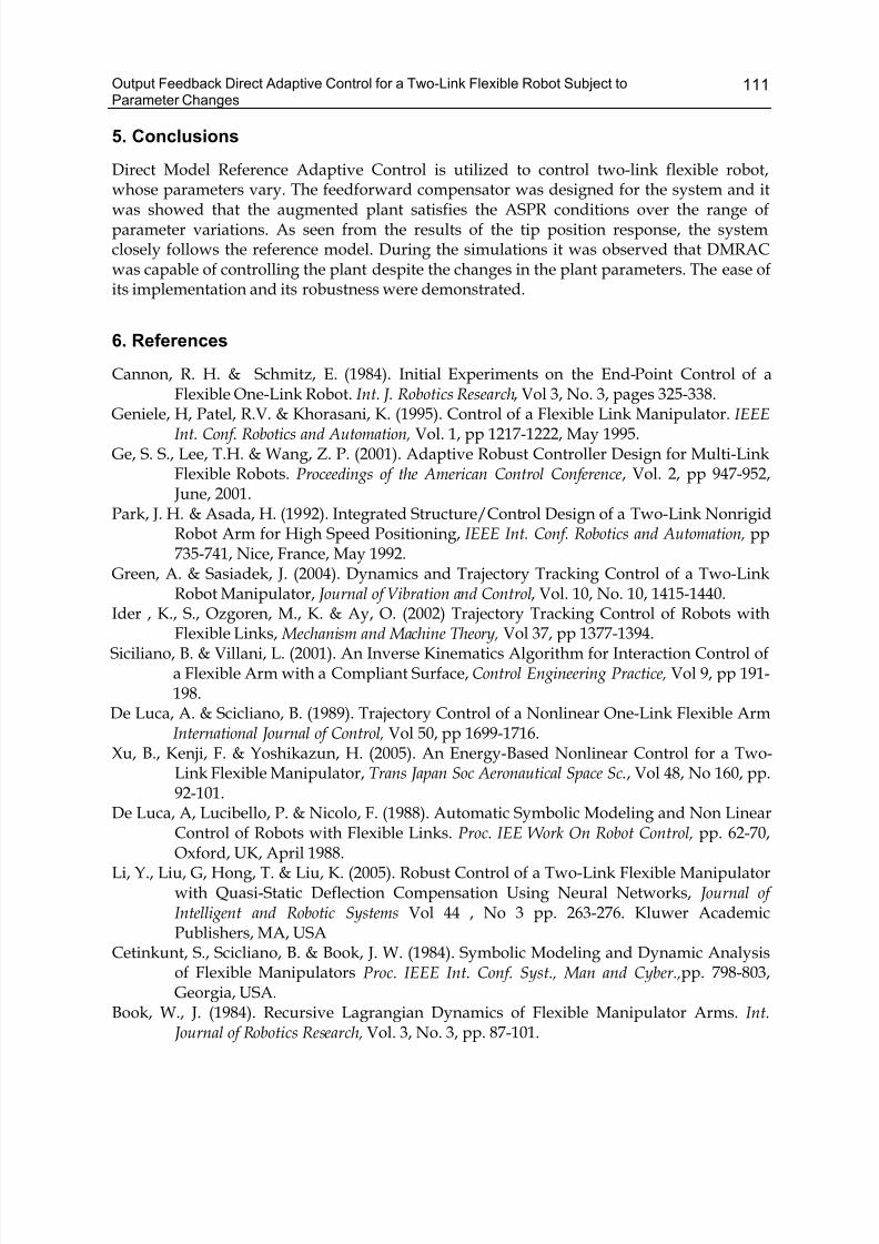
Output Feedback Direct Adaptive Control for a Two-Link Flexible Robot Subject toParameter Changes
111
5. Conclusions
Direct Model Reference Adaptive Control is utilized to control two-link flexible robot,whose parameters vary. The feedforward compensator was designed for the system and itwas showed that the augmented plant satisfies the ASPR conditions over the range ofparameter variations. As seen from the results of the tip position response, the systemclosely follows the reference model. During the simulations it was observed that DMRACwas capable of controlling the plant despite the changes in the plant parameters. The ease ofits implementation and its robustness were demonstrated.
6. References
Cannon, R. H. & Schmitz, E. (1984). Initial Experiments on the End-Point Control of aFlexible One-Link Robot. Int. J. Robotics Research, Vol 3, No. 3, pages 325-338.
Geniele, H, Patel, R.V. & Khorasani, K. (1995). Control of a Flexible Link Manipulator. IEEEInt. Conf. Robotics and Automation, Vol. 1, pp 1217-1222, May 1995.
Ge, S. S., Lee, T.H. & Wang, Z. P. (2001). Adaptive Robust Controller Design for Multi-LinkFlexible Robots. Proceedings of the American Control Conference, Vol. 2, pp 947-952, June, 2001.
Park, J. H. & Asada, H. (1992). Integrated Structure/Control Design of a Two-Link NonrigidRobot Arm for High Speed Positioning, IEEE Int. Conf. Robotics and Automation, pp735-741, Nice, France, May 1992.
Green, A. & Sasiadek, J. (2004). Dynamics and Trajectory Tracking Control of a Two-LinkRobot Manipulator, Journal of Vibration and Control, Vol. 10, No. 10, 1415-1440.
Ider , K., S., Ozgoren, M., K. & Ay, O. (2002) Trajectory Tracking Control of Robots withFlexible Links, Mechanism and Machine Theory, Vol 37, pp 1377-1394.
Siciliano, B. & Villani, L. (2001). An Inverse Kinematics Algorithm for Interaction Control ofa Flexible Arm with a Compliant Surface, Control Engineering Practice, Vol 9, pp 191-198.
De Luca, A. & Scicliano, B. (1989). Trajectory Control of a Nonlinear One-Link Flexible ArmInternational Journal of Control, Vol 50, pp 1699-1716.
Xu, B., Kenji, F. & Yoshikazun, H. (2005). An Energy-Based Nonlinear Control for a Two-Link Flexible Manipulator, Trans Japan Soc Aeronautical Space Sc., Vol 48, No 160, pp. 92-101.
De Luca, A, Lucibello, P. & Nicolo, F. (1988). Automatic Symbolic Modeling and Non LinearControl of Robots with Flexible Links. Proc. IEE Work On Robot Control, pp. 62-70,Oxford, UK, April 1988.
Li, Y., Liu, G, Hong, T. & Liu, K. (2005). Robust Control of a Two-Link Flexible Manipulatorwith Quasi-Static Deflection Compensation Using Neural Networks, Journal of Intelligent and Robotic Systems Vol 44 , No 3 pp. 263-276. Kluwer AcademicPublishers, MA, USA
Cetinkunt, S., Scicliano, B. & Book, J. W. (1984). Symbolic Modeling and Dynamic Analysisof Flexible Manipulators Proc. IEEE Int. Conf. Syst., Man and Cyber.,pp. 798-803,Georgia, USA.
Book, W., J. (1984). Recursive Lagrangian Dynamics of Flexible Manipulator Arms. Int. Journal of Robotics Research, Vol. 3, No. 3, pp. 87-101.
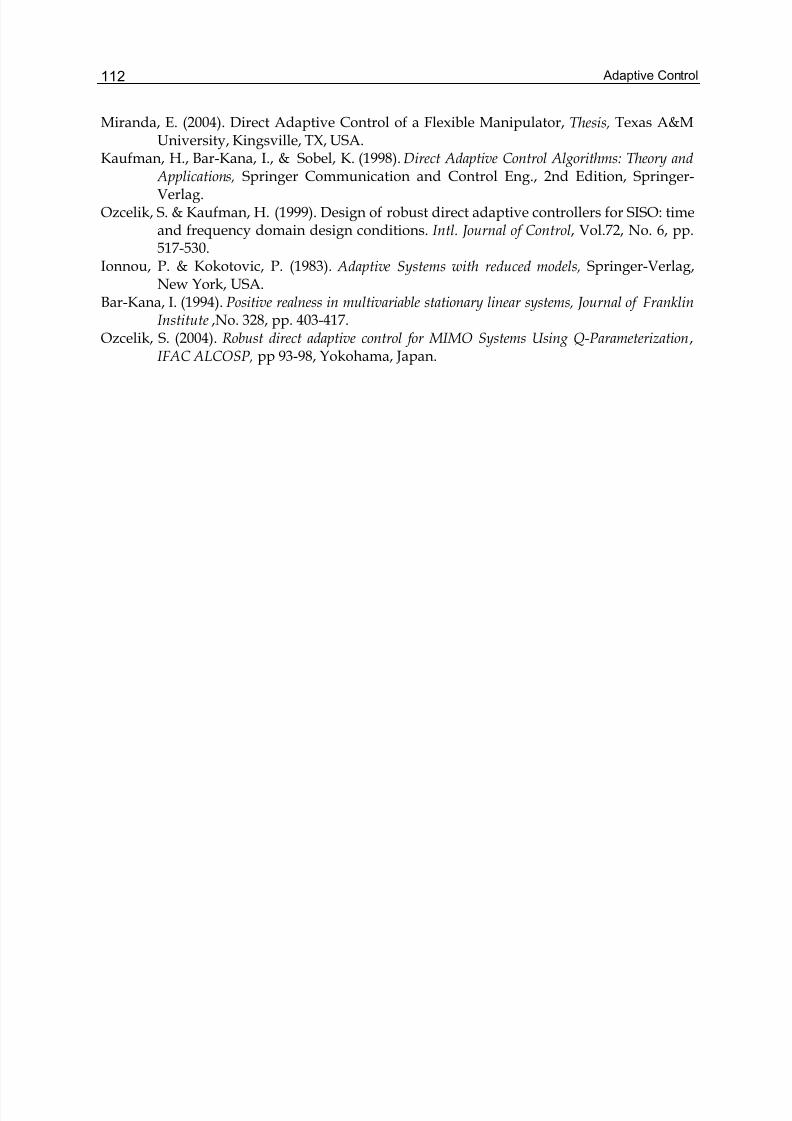
Adaptive Control112
Miranda, E. (2004). Direct Adaptive Control of a Flexible Manipulator, Thesis, Texas A&MUniversity, Kingsville, TX, USA.
Kaufman, H., Bar-Kana, I., & Sobel, K. (1998). Direct Adaptive Control Algorithms: Theory and Applications, Springer Communication and Control Eng., 2nd Edition, Springer-Verlag.
Ozcelik, S. & Kaufman, H. (1999). Design of robust direct adaptive controllers for SISO: timeand frequency domain design conditions. Intl. Journal of Control, Vol.72, No. 6, pp.517-530.
Ionnou, P. & Kokotovic, P. (1983). Adaptive Systems with reduced models, Springer-Verlag,New York, USA.
Bar-Kana, I. (1994). Positive realness in multivariable stationary linear systems, Journal of FranklinInstitute ,No. 328, pp. 403-417.
Ozcelik, S. (2004). Robust direct adaptive control for MIMO Systems Using Q-Parameterization,IFAC ALCOSP, pp 93-98, Yokohama, Japan.
5
Discrete Model Matching Adaptive Control for Potentially Inversely Non-Stable Continuous-
Time Plants by Using Multirate Sampling
S. Alonso-Quesada & M. De La SenElectricity and Electronics Department, Faculty of Science and Technology
Basque Country University, Spain
1. Introduction
Adaptive control theory has been widely applied for stabilizing linear time invariant plantsof unknown parameters (Goodwin & Sin, 1984). One of the more used methods for such apurpose is based on the model reference adaptive control (MRAC) problem (Aström &Wittenmark, 1997). Such a method requires some assumptions relative to the plant to becontrolled in order to carry out the synthesis of a stable controller (Narendra &Annaswamy, 1989). One of them is that the plant has to be inversely stable, what means thatits zeros have to be located within the stability domain. However, this information is notalways available to the designer when the system under control contains unknownparameters. There are several alternatives to circumvent this drawback and carry out thestable adaptive control design. Some of them consist on relaxing the control performancefrom the model matching to that achievable from the closed-loop pole placement (Alonso-Quesada & De la Sen, 2004 and Arvanitis, 1999). In this way, the stabilization of the closed-loop system can be ensured although its transient behaviour cannot be fixed to a predefinedone.
On one hand, the work (Alonso-Quesada & De la Sen, 2004) includes an estimatesmodification in the estimation algorithm to ensure the controllability of the estimated plantmodel without assuming any knowledge about the parameters of the plant to be controlled.This controllability property is crucial to avoid pole-zero cancellations between theestimated plant and the controller, which are both time-varying. In this context, a projectionof the estimated plant parameters into a region in the parameter space where the closed-loop system is free of pole-zero cancellations for all time can be alternatively used providedthat the true plant is controllable and the knowledge of a region where the true plantparameters belong to (Goodwin & Mayne, 1987).
On the other hand, the research (Arvanitis, 1999) proposes an adaptive pole-placementcontrol for linear systems using generalized sampled-data hold functions. Following such atechnique, gain controllers essentially need to be designed. Concretely, a periodic piecewiseconstant gain controller is added in the feedback chain. In the non-adaptive case, suchconstant gain values are those required so that the discretized closed-loop model under afundamental sampling period and a zero-order hold (ZOH) be stabilized. For such a
Adaptive Control114
purpose, each sampling period is divided in a certain finite number of uniform subintervalsand the controller gain takes a different value within each of them in order to locate thediscretized poles at the stable desired locations. In other words, the controller consists of aconstant vector of gains. In this sense, the controller works with a sampling rate faster thanthat used to discretize the plant to be controlled. In the adaptive case, an estimated model ofthe discretized plant is on-line updated by means of an estimation algorithm. Such a modelis used to parameterize the controller gains vector which becomes time-varying andconverges asymptotically to a constant one.
Another alternative, which does not relax the MRAC objective, to overcome thedrawback of the unstable zeros in a continuous-time plant is the design of discrete-timecontrollers which are synthesized from the discretization of the continuous-time plant bymeans of a holder device combined with a multirate with fast input sampling rate (De la Sen& Alonso-Quesada, 2007 and Liang & Ishitobi, 2004). The main motivation of this method isthat an inversely stable discretized model of the plant can be obtained with an appropriatechoice of the multirate gains. In this way, an adaptive controller can be designed to match adiscrete-time reference model since all the discretized plant zeros may be cancelled if suited.
In this context, a fractional-order hold (FROH) with a multirate input is used in this paper toobtain an inversely stable discretized plant model from a possible non-inversely stable and unstabletime invariant continuous-time plant. Then, a control design for matching a discrete-time referencemodel is developed for both non-adaptive and adaptive cases. Note that a FROH includes asparticular cases the ZOH and the FOH (first-order hold). In this way, the stabilization of thecontinuous-time plant is guaranteed without any assumption about the stability of its zerosand without requiring estimates modification in contrast with previous works on thesubject. In this sense, this paper is an extension of the work (De La Sen & Alonso-Quesada,2007) where the same problem is addressed. The main contribution is related to the method usedto built the continuous-time plant input from the discrete-time controller output. In the presentpaper, the FROH acts on the fundamental sampling period used to discretize the plant(plant output sampling) while in the aforementioned paper the FROH acted on the samplingperiod used to define the multirate device at the plant input. This later sampling period isan integer fraction of the plant output one, i.e. an integer number of input samples takesplace within each output sampling period. Such an integer has to be suitably chosen fordisposing of the enough freedom degrees being necessary to place the discretized plantzeros at desired locations, namely within the unity circle in order to guarantee the inversestability of the discretized plant model.
The assumptions about the plant to guarantee the closed-loop stability of the adaptivecontrol system are the following: (1) the stabilizability of the plant and (2) the knowledge ofthe continuous-time plant order. The motivation for using a multirate sampling inputinstead of the most conventional single rate one resides in the fact that the former, with theappropriate multirate gains, provides an inversely stable discretized plant model withoutrequirements on either the stability of the continuous-time plant zeros or the size of thesampling period. In this sense, a single rate input can only provide an inversely stablediscretized plant from an inversely stable continuous-time plant and, moreover, thefundamental sampling period to discretized the plant has to be sufficiently small (Blachuta,1999). Finally, the use of a FROH, instead of the most conventional ZOH, allows toaccommodate better some discrete adaptive techniques to the transient response of discrete-time controlled continuous-time plants (Bárcena et al., 2000 and Liang et al., 2003).
Discrete Model Matching Adaptive Control for Potentially Inversely Non-Stable Continuous-TimePlants by Using Multirate Sampling
115
The paper is organized as follows. Section 2 formulates a discrete state-spacedescription under fast input sampling to then obtain an input-output discrete transferfunction for the running slow sampling rate, namely, that acting on the output signal. Theselection of the scalar gains that generate the fast sampled input so that the discrete plantzeros are stable is focused on depending on the continuous-time plant parametrization.Section 3 discusses the synthesis of a model-matching based controller with a possiblepotential free design of all the zeros of the reference model. The case of known plantparameters and the adaptive case for not fully known plant parameters are both considered.Two alternatives are proposed to update on-line the time-varying multirate gains in theadaptive case. The first one updates the multirate gains for all sampling instants in order tomaintain the zeros of the estimated discretized plant fixed within the stability domain. Onthe contrary, the other one updates the multirate gains only when the change of gains iscrucial to guarantee the stability of the estimated discretized plant zeros. In this way, themultirate gains are not updated for all sampling instants and then they became piecewiseconstant. As a result, the zeros of the estimated discretized plant become time-varyingwithin the stability domain. Section 4 deals with the stability analysis of the adaptive controlsystem. Simulated examples which highlight the proposed design philosophy are providedin Section 5. A comparison of the results obtained with the two different methods forupdating the multirate gains is presented. Finally, conclusions end the paper in Section 6.
2. Discretized Plant Representation
Consider a linear time-invariant, single-input single-output and strictly proper continuous-time plant described by the following state space equations:
= + =&x(t) Ax(t) Bu(t) ; y(t) Cx(t) (1)
where u(t) and y(t) are, respectively, the input and output signals, ∈ℜnx(t) denotes the
state vector and A, B and C are constant matrices of suitable dimensions. A FROH and amultirate sampling on the fast input sampling will be used in order to obtain an inverselystable discretized plant model. The signal generated by such a device is given by,
( )− −⎧ ⎫= α + β −⎨ ⎬
⎩ ⎭ j
u(k) u(k 1)u(t) u(k) t kT
T(2)
for [ )′ ′∈ + − +t kT ( j 1)T ,kT jT , ∈ K j 1, 2, , N and FROH correcting gain [ ) ( ]β∈ − ∪1,0 0,1 ,
where T is the sampling period (slow sampling) which is divided in N equal subperiods of
length ′ = TT N (fast sampling) to generate the multirate plant input, u(k) denotes the
value of a discrete-time controller output signal at the instant kT, for all non-negative
integer k, and α j ’s are real constants. Note that the FROH device operates on the sequence
u(k) defined at the slow sampling instants kT and then the input u(t) is generated over
each subperiod with the corresponding gain α j , for ∈ K j 1, 2, , N , via (2). By substituting
(2) into (1) and sampling the plant output y(t) over the sampling period T, the following
Adaptive Control116
state space representation is obtained which corresponds to the discrete-time plant model
that relates the sequences u(k) and y(k) :
+ = + + − =1 2x(k 1) F x(k) G u(k) G u(k 1) ; y(k) C x(k) (3)
where = ψ = φ =N ATF (T) e is the continuous-time state transition matrix computed for a
slow sampling period and,
− × − ×
= =
β β⎛ ⎞ ⎛ ⎞⎛ ⎞′ ′= α ψ Γ + Γ ∈ℜ = − α ψ Γ ∈ℜ⎜ ⎟⎜ ⎟ ⎜ ⎟⎝ ⎠⎝ ⎠ ⎝ ⎠
∑ ∑l l
l l
l l
N NN n 1 N n 1
1 21 1
G ; GT T
(4)
with,
′ ′× ×′ ′ ′Γ = φ − ∈ℜ Γ = φ − ∈ℜ∫ ∫
T Tn 1 n 1
0 0(T s) B ds ; (T s) B s ds (5)
The transfer function of this discrete-time plant model is,
− ⎛ ⎞= − ψ + =⎜ ⎟⎝ ⎠
N 1n 1 2
1 B(z)H(z) C(zI ) G G
z A(z)(6)
where,
+Δ − +
Δ=
+ − +
=
⎡ ⎤− ψ= − ψ = ⎢ ⎥−⎣ ⎦
= − ψ = +
∑
∑
N n 1nN n i 1
n ii 1
nN n 1 n i 1
n ii 1
zI C (z)gB(z) C Adj(zI )C (z)g Det = b z
C 0
A(z) z Det(zI ) z a z
(7)
with ⋅Adj( ) and ⋅Det( ) denoting, respectively, the adjoint matrix and the determinant of the
square matrix (.), nI denoting the n-th order identity matrix, and
[ ]
ΓT
βΓ
T
βΓzΔ(z)
Δ(z)ψΔ(z)Δ(z)ψ(z)C;ααg nxN1 N
Δ
1 NT
N1
′−⎟ ⎠
⎞⎜⎝
⎛ ′+=
ℜ∈ℜ∈= −+LLL
(8)
Note that the coefficients ib , for ∈ +Ki 1, 2, , n 1 , of the polynomial B(z) in (7)
depend on the values α j , for ∈ … j 1, 2, , N , which define the multirate device. This fact
lets to allocate the zeros of the discretized plant model at desired locations if a suitable
number of multirate gains is provided. In this sense, the multirate gains α j , being the
components of the vector g , are calculated to guarantee that such zeros are maintained
within the stability domain, i.e., the unity circle. In particular, the coefficients ib can be
Discrete Model Matching Adaptive Control for Potentially Inversely Non-Stable Continuous-TimePlants by Using Multirate Sampling
117
expressed as:
=
= α ⇔ =∑N
i i , j j j 1
b b v M g (9)
where + ×⎡ ⎤= ∈ℜ⎣ ⎦(n 1) N
i , jM b and [ ]+= KT
1 2 n 1v b b b . The coefficients i , jb depend on the
parameters of the continuous-time plant, the sampling period T and the correcting gain β of
the FROH considered in the discretization process.
Assumptions 1. (i) The plant is stabilizable, i.e. its transfer function does not possess unstable pole-zero
cancellations,(ii) the plant order n is known, and
(iii) the correcting gain β of the FROH device and the sampling period T are chosen such
that M is a full rank matrix. ***
Remark 1. The multirate gains vector g required to place the zeros of the discretized plant
transfer function (6) at desired locations may be calculated from (9) provided Assumptions 1
and that ≥ +N n 1 . In this sense, such locations are prefixed via a suitable choice of the
vector v composed by the coefficients of the desired polynomial for the transfer function
numerator. If > +N n 1 , different solutions can be obtained for g . Otherwise, i.e. if
= +N n 1 , there is a unique solution for the multirate gains vector from the linear algebraic
system (9) which places the discretized zeros at desired locations. ***
The discretized model (6) can be described by the following difference equation:
+ +
= = = = =
+
= = =
= − − + − = − − + α −
= − − + − = θ ϕ −
∑ ∑ ∑ ∑∑
∑ ∑∑
n n 1 n n 1 N
i i i i , j ji 1 i 1 i 1 i 1 j 1
n n 1 NT
i i , j ji 1 i 1 j 1
y(k) a y(k i) b u(k i) a y(k i) b u(k i)
a y(k i) b u (k i) (k 1)
(10)
where,
[ ] [ ]
[ ]
+ ⎡ ⎤⎡ ⎤θ = θ θ θ θ ϕ − = ϕ − ϕ − ϕ − ϕ − −⎣ ⎦ ⎣ ⎦
θ = − − − ϕ − = − − −
θ = ϕ − = − − −⎡ ⎤⎣ ⎦− =
K K
K K
K K
TTT T T T T T T Ta y u u ub,1 b,2 b,n 1
T T
a 1 2 n y
T T
i ,1 i ,2 i ,N u 1 2 Nb,i
j
; (k 1) (k 1) (k 1) (k 2) (k n 1)
a a a ; (k 1) y(k 1) y(k 2) y(k n)
b b b ; (k i) u (k i) u (k i) u (k i)
u (k i) α − ju(k i)
(11)
for all ∈ +Ki 1, 2, , n 1 and all ∈ K j 1, 2, , N . In the rest of the paper, the case
= +N n 1 will be considered for simplicity purposes.
Adaptive Control118
3. Control Design
The control objective in the case of known plant parameters is that the discretized plant
model matches a stable discrete-time reference model = mm
m
B (z)H (z)
A (z)whose zeros can be
freely chosen, where z is the Z-transform argument. Such an objective is achievable if thediscretization process uses the multirate sampling input with the appropriate multirategains, what guarantees the inverse stability of the discretized plant. Then, all the discretizedplant zeros may be cancelled by controller poles. In this way, the continuous-time plantoutput tracks the reference model output at the sampling instants. The tracking-errorbetween such signals is zero at all sampling instants in the case of known plant parameterswhile it is maintained bounded for all time while it converges asymptotically to zero as timetends to infinity in the adaptive case considered when the plant parameters are fully orpartially unknown. A self-tuning regulator scheme is used to meet the control objective inboth non-adaptive and adaptive cases.
3.1 Known PlantThe proposed control law is obtained from the difference equation:
= −R(q) u(k) T(q) c(k) S(q) y(k) (12)
for all non-negative integer k, where c(k) is the input reference sequence and q is the
running sample rate advance operator being formally equivalent to the Z-argument used indiscrete transfer functions. The reconstruction of the continuous-time plant input u(t) is
made by using (2), with the control sequence u(k) obtained from (12), with the
appropriate multirate gains α j , for ∈ K j 1, 2, , N , to guarantee the stability of the
discretized plant zeros.The discrete-time transfer function of the closed-loop system obtained from the
application of the control law (12) to the discretized plant (6) is given by:
= =+ +
Y(z) B(z)T(z) T(z)
C(z) A(z)R(z) B(z)S(z) A(z) S(z)(13)
where the second equality is fulfilled if the control polynomial =R(z) B(z) . In this way, the
polynomial B(z) , which is stable, is cancelled. Then, the polynomials T(z) , R(z) and S(z)
of the controller (12) so that = m
m
Y(z) B (z)
C(z) A (z)are obtained from:
= = = −m s m sT(z) B (z)A (z) ; R(z) B(z) ; S(z) A (z)A (z) A(z) (14)
where sA (z) is a stable monic polynomial of zero-pole cancellations of the closed-loop
system. The following degree constraints are satisfied in the synthesis of the controller:
Discrete Model Matching Adaptive Control for Potentially Inversely Non-Stable Continuous-TimePlants by Using Multirate Sampling
119
[ ] [ ] [ ]
[ ] [ ]
[ ] [ ] [ ]
−+
=
⎧ + = = +⎪⎪ = − = ⇒ =⎨⎪⎪ = + ≤⎩
∑
m s
nn i
i 1i 0
m s
Deg A (z) Deg A (z) Deg A(z) n 1
Deg S(z) Deg A(z) 1 n S(z) s z
Deg T(z) Deg B (z) Deg A (z) n
(15)
3.2 Unknown Plant
If the continuous-time plant parameters are unknown then the vector θ in (11) composed of
the discretized plant model parameters is also unknown. However, all the above controldesign in the previous subsection remains valid if such a parameter vector is estimated byan estimation algorithm. In this way, the controller parameterization can be obtained from
= ˆR(z,k) B(z,k) , with B(z,k) denoting the estimated of B(z) at the current slow sampling
instant kT, and equations similar to (14) by replacing the discretized plant polynomial A(z)
by its corresponding estimated one A(z,k) (Alonso-Quesada & De la Sen, 2004). Note that
T(z) in (14) has to be calculated once for all since mB (z) and sA (z) are time-invariant while
S(z) is updated at each running sampling time since the polynomial A(z,k) is time-
varying. The coefficients of the unknown polynomial B(z) depend, via (9), on the multirate
input gains α j , for ∈ K j 1, 2, , N , being applicable to calculate the input within the inter-
sample slow period. However, the estimation algorithm provides an adaptation of each
parameter i , jb , namely i, jb (k) , for ∈ Ki, j 1, 2, , N and all non negative integer k. Then,
the α j -gains have to be also updated in order to ensure the stability of the zeros of the
estimated discretized plant, i.e. the roots of B(z,k) be stable. Then, the gains α j become
time-varying, namely α jˆ (k) . The estimation algorithm for updating the parameters vector
θ(k) , which denotes the estimated of θ , and two different design alternatives for the
adaptation of the multirate gains are presented below. Also, the main boundedness andconvergence properties derived from the use of such algorithms are established.
3.2.1. Estimation algorithmAn ‘a priori’ estimated parameters vector is obtained at each slow sampling instant by usinga recursive least-squares algorithm (Goodwin & Sin, 1984) defined by:
− ϕ − ϕ − −= − −
+ ϕ − − ϕ −
− ϕ −θ = θ − +
+ ϕ − − ϕ −
T
T
00 0
T
P(k 1) (k 1) (k 1) P(k 1)P(k) P(k 1)
1 (k 1) P(k 1) (k 1)
P(k 1) (k 1) e (k)ˆ ˆ(k) (k 1)1 (k 1) P(k 1) (k 1)
(16)
for all integer >k 0 where ( )= θ − θ − ϕ − = θ − ϕ −%T T0 0 0ˆe (k) (k 1) (k 1) (k 1) (k 1) denotes the ‘a
priori’ estimation error and P(k) is the covariance matrix initialized as = >TP(0) P (0) 0 .
Adaptive Control120
Such an algorithm provides an estimation θ0ˆ (k) of the parameters vector by using the
regressor ϕ −(k 1) , defined in (11), built with the output and input measurements with the
multirate gains α − jˆ (k 1) obtained at the previous slow sampling instant, i.e.
− = α − − j jˆu (k i) (k 1) u(k i) for all ∈ Ki 1, 2, , n+1 . Then, an ‘a posteriori’ estimates vector
is obtained in the following way:
Modification algorithm. This algorithm consists of three steps:
Step 1: Built the matrix ×⎡ ⎤= ∈ℜ⎣ ⎦0 0 N N
i, jˆM (k) b (k) , for ∈ Ki , j 1, 2, , N , from the ‘a priori’
estimates θ0b, i
ˆ (k) , included in θ 0ˆ (k) , of the corresponding θb, i defined in (11).
Step 2: = 0ˆ ˆM(k) M (k)
If ⎡ ⎤ ≥ δ⎣ ⎦ 0ˆDet M(k) then θ = θ0
b,i b,iˆ ˆ(k) (k)
else while ⎡ ⎤ < δ⎣ ⎦ 0ˆDet M(k)
= + δ Nˆ ˆM(k) M(k) I
end;
for =i 1 to N
θ = ib, iˆ ˆ(k) M (k)
endend.
Step 3: ⎡ ⎤θ = θ θ θ θ⎣ ⎦KTT0 T T T
a b,1 b,2 b,Nˆ ˆ ˆ ˆ ˆ(k) (k) (k) (k) (k) ,
for some real positive constants δ << 1 and δ <<0 1 , and where iM (k) denotes the i-th row
of M(k) . ***
Remark 2. Note that the estimate θ0a
ˆ (k) corresponding to the parameters of θa is not
affected by the modification algorithm. Also, note that the while instruction part of the
second step is doing a finite number of times since there exists a finite integer number l
such that ( ) ( )⎡ ⎤ ⎡ ⎤= + δ = δ + δ θ θ θ ≥ δ⎣ ⎦ ⎣ ⎦l l KN0 0 0 0
N 0b,1 b,2 b,Nˆ ˆ ˆ ˆ ˆDet M(k) Det M (k) I f , (k), (k), , (k) . ***
3.2.2. Updating of the time-varying multirate gains
Once the estimated parameters vector is obtained at each slow sampling instant themultirate input gains have to be updated. Two alternative algorithms are considered tocarry out such an operation.
Algorithm 1.A vector of multirate gains is updated at all slow sampling instants in order to maintain thezeros of the estimated discretized plant fixed at desired locations within the stability domain
<z 1 . Such desired zeros are the roots of a predefined polynomial ′B(z) . For such a
Discrete Model Matching Adaptive Control for Potentially Inversely Non-Stable Continuous-TimePlants by Using Multirate Sampling
121
purpose, the required vector g(k) is obtained from the resolution of the following matrix
equation:
=ˆ ˆM(k) g(k) v (17)
at each slow sampling instant, where [ ]′ ′ ′= KT
1 2 Nv b b b is composed by the coefficients
of ′B(z) , ×⎡ ⎤= ∈ℜ⎣ ⎦N N
i, jˆM(k) b (k) , with i , jb (k) denoting each of the ‘a posteriori’ estimated
parameters corresponding to the components of the vectors θb, i defined in (11), and
[ ]= α α αKT
1 2 Nˆ ˆ ˆ ˆg(k) (k) (k) (k) . In this way, g(k) is composed by the multirate gains
which make the numerator of the estimated discretized plant model be equal to the desiredpolynomial ′B(z) . Note that the matrix equation (17) can be solved at all slow sampling
instants since the parameters modification added to the estimation algorithm ensures the
non-singularity of the matrix M(k) .
Algorithm 2.It consists of solving the equation (17) only when it is necessary to modify the previousvalues of the multirate gains in order to guarantee the stability of the zeros of the estimateddiscretized plant model. i.e., the multirate gains remain equal to those of the preceding slowsampling instant if the zeros of the estimated discretized plant obtained with the current
estimated parameters vector, θ(k) , and the previous multirate gains, α − jˆ (k 1) , are within
the discrete-time stability domain. Otherwise, the multirate gains are updated by theresolution of the equation (17), which can be solved whenever it is necessary since the
matrix M(k) is invertible at all slow sampling instant due to the modification included in
the estimation algorithm. In this way, the multirate gains are piecewise constant, theestimated discretized plant zeros are time-varying and the computational burden associatedwith the updating of the multirate gains is reduced with respect to that of Algorithm 1.
3.2.3. Properties of the estimated modelsThe parameter estimation algorithm, together with any of the considered adaptationalgorithms for the multirate gains, possesses the properties given in the following lemma,whose proof is presented in Appendix A.
Lemma 1. Main properties of the estimation and multirate gains adaptation algorithms
(i) P(k) is uniformly bounded for all non-negative integer k, and it asymptotically
converges to a finite, at least semidefinite positive, limit as → ∞k .
(ii) θ 0ˆ (k) and θ(k) are uniformly bounded and they asymptotically converge to a finite
limit as → ∞k .
(iii) The vector g(k) of multirate gains is bounded and converges to a finite limit as → ∞k .
(iv)( )
+ ϕ − − ϕ −
20
T
e (k)
1 (k 1) P(k 1) (k 1)is uniformly bounded and it asymptotically converges to
Adaptive Control122
zero as → ∞k .
(v) 0e (k) asymptotically converges to zero as → ∞k .
(vi) Assuming that the external input c(k) is sufficiently rich such that ϕ −(k 1) in (11) is
persistently exciting, θ0ˆ (k) tends to the true parameters vector θ as → ∞k . Then, θ(k)
tends to θ 0ˆ (k) and ( )= θ − θ − ϕ −Tˆe(k) (k 1) (k 1) tends to zero as → ∞k . ***
Remark 3. The convergence of the estimated parameters to their true values in θ requires
that ϕ −(k 1) is persistently exciting. In this context, ϕ −(k 1) is persistently exciting if there
exists an integer l such that+
=
ρ > ϕ − ϕ − > ρ∑l0
0
kT
1 m 2 mk k
I (k 1) (k 1) I where ρ >1 0 , ρ >2 0 and
= + = + +2 2m n N n 3n 1 is the number of components of the regressor ϕ −(k 1) . Such a
condition may be ensured by chosing an external input sufficiently rich of order m , i.e. it
consists of at least m2 frequencies in the frequency domain (Ioannou & Sun, 1996). ***
4. Stability Analysis
The plant discretized model can be written as follows,
+
= =
= + = θ − ϕ − + = − − − + − − +∑ ∑n n 1
Ti i
i 1 i 1
ˆˆ ˆˆy(k) y(k) e(k) (k 1) (k 1) e(k) a (k 1)y(k i) b (k 1)u(k i) e(k) (18)
and the adaptive control law as,
( ) ( )+ += =
+
+=
⎧= − − − − − − − − + − −⎨
⎩
⎫− − − − − + − + − + δ⎬
⎭
∑ ∑
∑ i
n n
1 i i 1 1 i i 1i 1 i 11
n 11
1 n 1 mi 1 1
1 ˆ ˆˆ ˆ ˆ ˆu(k) s (k 1)a (k 1) s (k 1) y(k i) s (k 1)b (k 1) b (k 1) u(k i)b (k)
s (k)ˆs (k 1)b (k 1)u(k n 1) b c(k i 1) e(k) (k)b (k)
(19)
where (12) has been used with R(q) and S(q) substituted, respectively, by time-varying
polynomials =ˆ ˆR(z, k) B(z, k) and S(z,k) , which is the solution of the equation (14) for the
adaptive case, and,
( ) ( )
( ) ( )
( )
+ +=
+ +=
+
⎧δ = ⎡ − − − − − − ⎤ −⎨ ⎣ ⎦
⎩
⎡ ⎤− − − − + − − −⎣ ⎦
− − − −
∑
∑
n
1 1 i i 1 i 1i 11
n
1 1 i i 1 i 1i 1
1 1 n 1
1ˆ ˆ ˆ ˆ ˆ(k) s (k) s (k 1) a (k 1) s (k) s (k 1) y(k i)
b (k)
ˆ ˆ ˆˆ ˆs (k) s (k 1) b (k 1) b (k) b (k 1) u(k i)
ˆˆ ˆs (k) s (k 1) b (k − −1)u(k n 1)
(20)
By combining (18) and (19), the discrete-time closed-loop system can be written as:
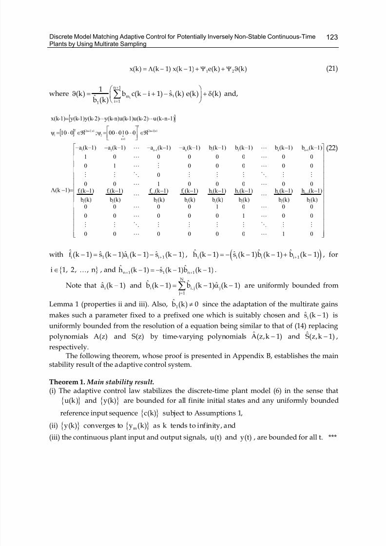
Discrete Model Matching Adaptive Control for Potentially Inversely Non-Stable Continuous-TimePlants by Using Multirate Sampling
123
= Λ − − + Ψ + Ψ ϑ1 2x(k) (k 1) x(k 1) e(k) (k) (21)
where+
=
⎛ ⎞ϑ = − + − + δ⎜ ⎟
⎝ ⎠∑ i
n 1
m 1i 11
1ˆ(k) b c(k i 1) s (k) e(k) (k)
b (k)and,
[ ]
[ ] ( )
( )
⎥⎥⎥⎥⎥⎥⎥⎥⎥⎥⎥⎥⎥⎥⎥
⎦
⎤
⎢⎢⎢⎢⎢⎢⎢⎢⎢⎢⎢⎢⎢⎢⎢
⎣
⎡
−−−−−−−−
−−−−−−−−−−−−
=−
ℜ∈⎥⎦⎤
⎢⎣⎡=ℜ∈=
=
+
+−
+
+
+
01000000
00100000
00010000
(k) b
1)(k h
(k) b
1)(k h
(k) b
1)(k h
(k) b
1)(k h
(k) b
1)(k f
(k) b
1)(k f
(k) b
1)(k f
(k) b
1)(k f 00000100
0
0000010
00000001
1)(k b1)(k b1)(k b1)(k b1)(k a1)(k a1)(k a1)(k a
1)Λ(k
001000ψ;010ψ
1)-n-(k u2)-u(k 1)-u(k n)-y(k 2)-y(k 1)-y(k 1)-x(k
1
1n
1
n
1
2
1
1
1
n
1
1-n
1
1
1
1
1nn21n1n21
x112n
T
1n
2
x112nT
1
LL
MMOMMMMOMM
LL
LL
LL
LL
MMOMMMOMM
LML
LL
LL
LLL
LL
ˆ
ˆ
ˆ
ˆ
ˆ
ˆ
ˆ
ˆ
ˆ
ˆ
ˆ
ˆ
ˆ
ˆ
ˆ
ˆ
ˆ ˆ ˆ ˆ ˆ ˆ ˆ ˆ (22)
with +− = − − − −i 1 i i 1ˆ ˆ ˆ ˆf (k 1) s (k 1)a (k 1) s (k 1) , ( )+− = − − − + −i i i i 1
ˆ ˆ ˆˆh (k 1) s (k 1)b (k 1) b (k 1) , for
∈ …i 1, 2, , n , and + +− = − − −n 1 1 n 1ˆ ˆˆh (k 1) s (k 1)b (k 1) .
Note that −ia (k 1) and=
− = − α −∑N
i i , j j j 1
ˆ ˆ ˆb (k 1) b (k 1) (k 1) are uniformly bounded from
Lemma 1 (properties ii and iii). Also, ≠1b (k) 0 since the adaptation of the multirate gains
makes such a parameter fixed to a prefixed one which is suitably chosen and −is (k 1) is
uniformly bounded from the resolution of a equation being similar to that of (14) replacing
polynomials A(z) and S(z) by time-varying polynomials −A(z,k 1) and −S(z,k 1) ,
respectively.The following theorem, whose proof is presented in Appendix B, establishes the main
stability result of the adaptive control system.
Theorem 1. Main stability result. (i) The adaptive control law stabilizes the discrete-time plant model (6) in the sense that
u(k) and y(k) are bounded for all finite initial states and any uniformly bounded
reference input sequence c(k) subject to Assumptions 1,
(ii) y(k) converges to my (k) as k tends to infinity, and
(iii) the continuous plant input and output signals, u(t) and y(t) , are bounded for all t. ***
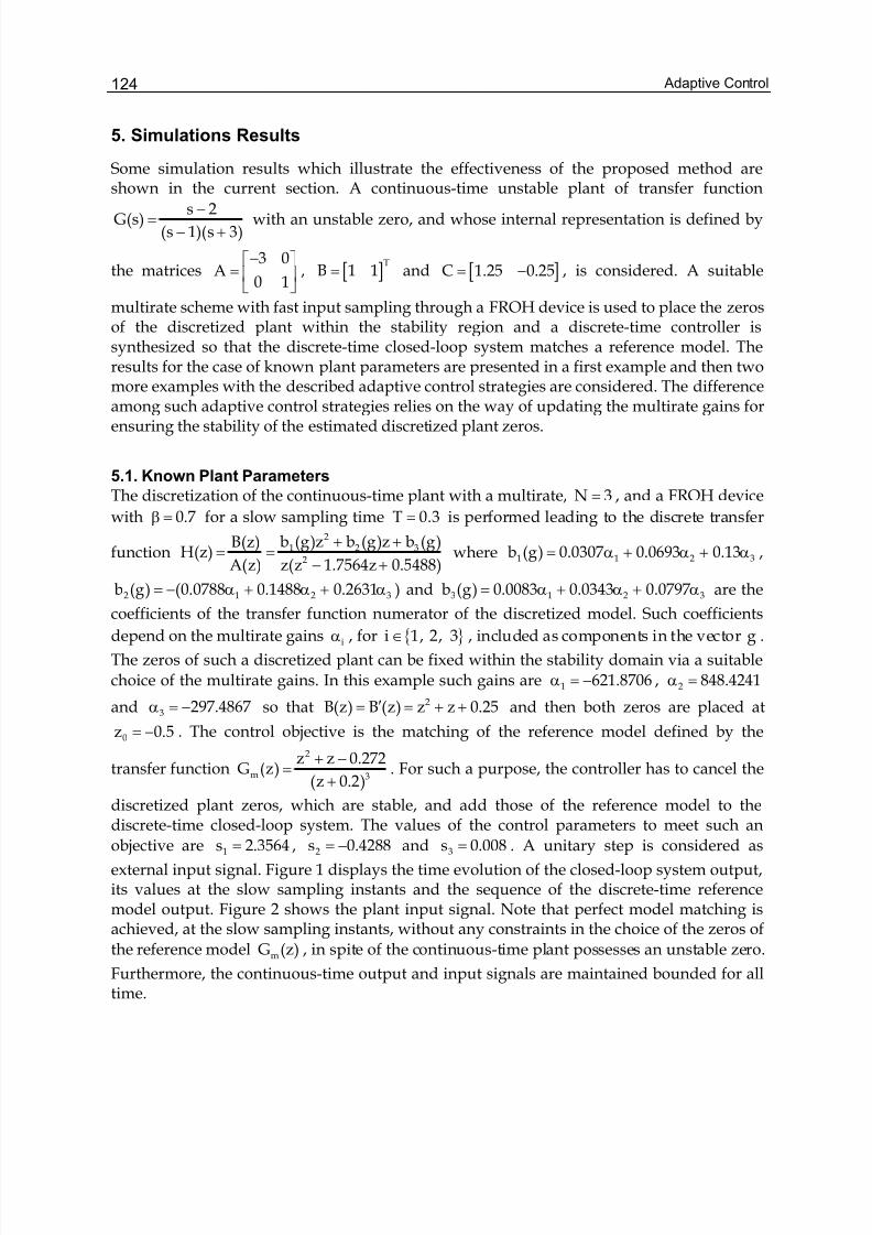
Adaptive Control124
5. Simulations Results
Some simulation results which illustrate the effectiveness of the proposed method areshown in the current section. A continuous-time unstable plant of transfer function
−=
− +s 2
G(s)(s 1)(s 3)
with an unstable zero, and whose internal representation is defined by
the matrices−⎡ ⎤
= ⎢ ⎥⎣ ⎦
3 0A
0 1, [ ]=
TB 1 1 and [ ]= −C 1.25 0.25 , is considered. A suitable
multirate scheme with fast input sampling through a FROH device is used to place the zerosof the discretized plant within the stability region and a discrete-time controller issynthesized so that the discrete-time closed-loop system matches a reference model. Theresults for the case of known plant parameters are presented in a first example and then twomore examples with the described adaptive control strategies are considered. The differenceamong such adaptive control strategies relies on the way of updating the multirate gains forensuring the stability of the estimated discretized plant zeros.
5.1. Known Plant Parameters
The discretization of the continuous-time plant with a multirate, =N 3 , and a FROH device
with β = 0.7 for a slow sampling time =T 0.3 is performed leading to the discrete transfer
function+ +
= =− +
21 2 3
2
b (g)z b (g)z b (g)B(z)H(z)
A(z) z(z 1.7564z 0.5488)where = α + α + α1 1 2 3b (g) 0.0307 0.0693 0.13 ,
= − α + α + α2 1 2 3b (g) (0.0788 0.1488 0.2631 ) and = α + α + α3 1 2 3b (g) 0.0083 0.0343 0.0797 are the
coefficients of the transfer function numerator of the discretized model. Such coefficients
depend on the multirate gains αi , for ∈i 1, 2, 3 , included as components in the vector g .
The zeros of such a discretized plant can be fixed within the stability domain via a suitable
choice of the multirate gains. In this example such gains are α = −1 621.8706 , α =2 848.4241
and α = −3 297.4867 so that ′= = + +2B(z) B (z) z z 0.25 and then both zeros are placed at
= −0z 0.5 . The control objective is the matching of the reference model defined by the
transfer function+ −
=+
2
m 3
z z 0.272G (z)
(z 0.2). For such a purpose, the controller has to cancel the
discretized plant zeros, which are stable, and add those of the reference model to thediscrete-time closed-loop system. The values of the control parameters to meet such an
objective are =1s 2.3564 , = −2s 0.4288 and =3s 0.008 . A unitary step is considered as
external input signal. Figure 1 displays the time evolution of the closed-loop system output,its values at the slow sampling instants and the sequence of the discrete-time referencemodel output. Figure 2 shows the plant input signal. Note that perfect model matching isachieved, at the slow sampling instants, without any constraints in the choice of the zeros of
the reference model mG (z) , in spite of the continuous-time plant possesses an unstable zero.
Furthermore, the continuous-time output and input signals are maintained bounded for alltime.
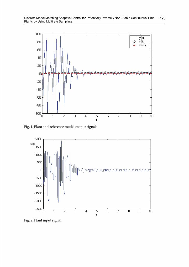
Discrete Model Matching Adaptive Control for Potentially Inversely Non-Stable Continuous-TimePlants by Using Multirate Sampling
125
Fig. 1. Plant and reference model output signals
Fig. 2. Plant input signal
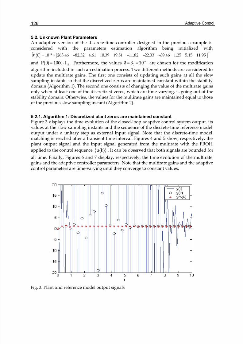
Adaptive Control126
5.2. Unknown Plant ParametersAn adaptive version of the discrete-time controller designed in the previous example isconsidered with the parameters estimation algorithm being initialized with
[ ]−θ = × − − − −T0 2ˆ (0) 10 263.46 82.32 4.61 10.39 19.51 11.82 22.33 39.46 1.25 5.15 11.95
and = ⋅ 11P(0) 1000 I . Furthermore, the values −δ = δ = 60 10 are chosen for the modification
algorithm included in such an estimation process. Two different methods are considered toupdate the multirate gains. The first one consists of updating such gains at all the slowsampling instants so that the discretized zeros are maintained constant within the stabilitydomain (Algorithm 1). The second one consists of changing the value of the multirate gainsonly when at least one of the discretized zeros, which are time-varying, is going out of thestability domain. Otherwise, the values for the multirate gains are maintained equal to thoseof the previous slow sampling instant (Algorithm 2).
5.2.1. Algorithm 1: Discretized plant zeros are maintained constantFigure 3 displays the time evolution of the closed-loop adaptive control system output, itsvalues at the slow sampling instants and the sequence of the discrete-time reference modeloutput under a unitary step as external input signal. Note that the discrete-time modelmatching is reached after a transient time interval. Figures 4 and 5 show, respectively, theplant output signal and the input signal generated from the multirate with the FROH
applied to the control sequence u(k) . It can be observed that both signals are bounded for
all time. Finally, Figures 6 and 7 display, respectively, the time evolution of the multirategains and the adaptive controller parameters. Note that the multirate gains and the adaptivecontrol parameters are time-varying until they converge to constant values.
Fig. 3. Plant and reference model output signals
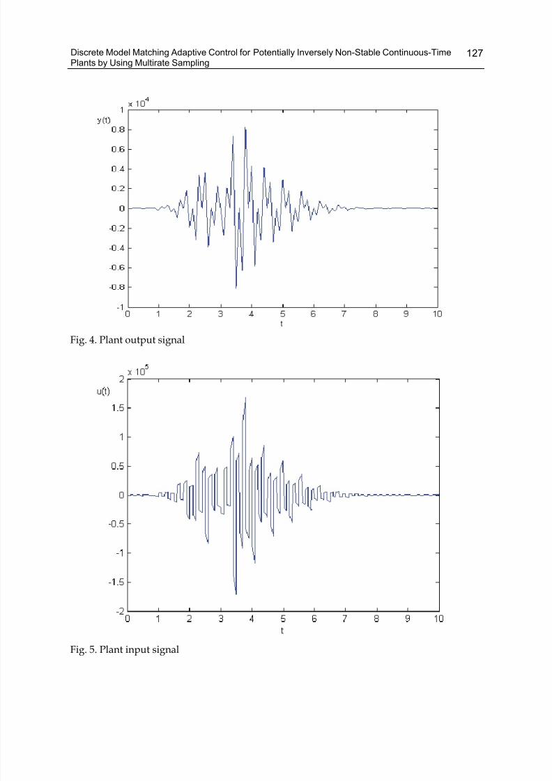
Discrete Model Matching Adaptive Control for Potentially Inversely Non-Stable Continuous-TimePlants by Using Multirate Sampling
127
Fig. 4. Plant output signal
Fig. 5. Plant input signal
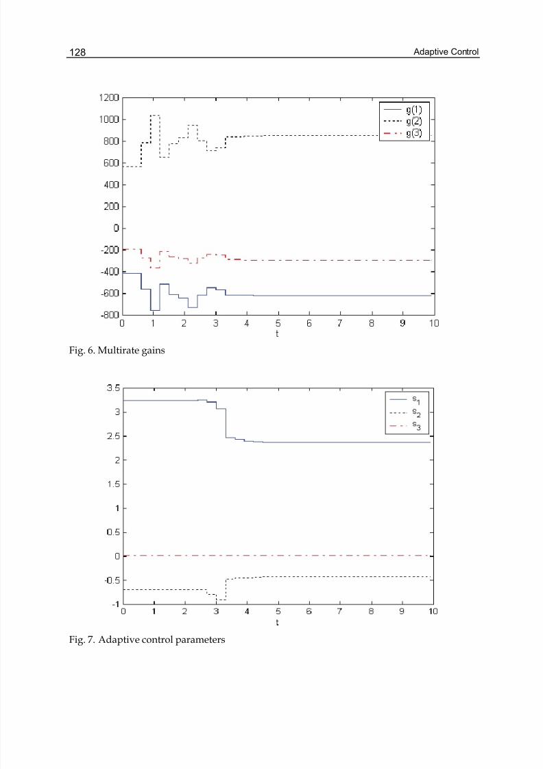
Adaptive Control128
Fig. 6. Multirate gains
Fig. 7. Adaptive control parameters
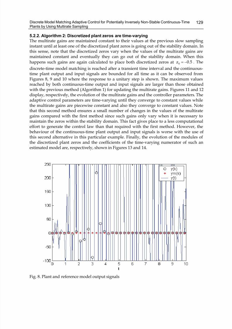
Discrete Model Matching Adaptive Control for Potentially Inversely Non-Stable Continuous-TimePlants by Using Multirate Sampling
129
5.2.2. Algorithm 2: Discretized plant zeros are time-varyingThe multirate gains are maintained constant to their values at the previous slow samplinginstant until at least one of the discretized plant zeros is going out of the stability domain. Inthis sense, note that the discretized zeros vary when the values of the multirate gains aremaintained constant and eventually they can go out of the stability domain. When this
happens such gains are again calculated to place both discretized zeros at = −0z 0.5 . The
discrete-time model matching is reached after a transient time interval and the continuous-time plant output and input signals are bounded for all time as it can be observed fromFigures 8, 9 and 10 where the response to a unitary step is shown. The maximum valuesreached by both continuous-time output and input signals are larger than those obtainedwith the previous method (Algorithm 1) for updating the multirate gains. Figures 11 and 12display, respectively, the evolution of the multirate gains and the controller parameters. Theadaptive control parameters are time-varying until they converge to constant values whilethe multirate gains are piecewise constant and also they converge to constant values. Notethat this second method ensures a small number of changes in the values of the multirategains compared with the first method since such gains only vary when it is necessary tomaintain the zeros within the stability domain. This fact gives place to a less computationaleffort to generate the control law than that required with the first method. However, thebehaviour of the continuous-time plant output and input signals is worse with the use ofthis second alternative in this particular example. Finally, the evolution of the modules ofthe discretized plant zeros and the coefficients of the time-varying numerator of such anestimated model are, respectively, shown in Figures 13 and 14.
Fig. 8. Plant and reference model output signals
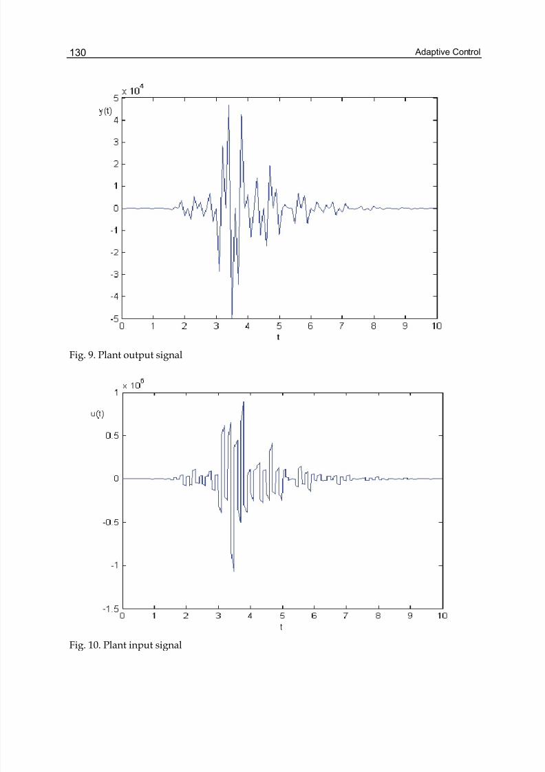
Adaptive Control130
Fig. 9. Plant output signal
Fig. 10. Plant input signal
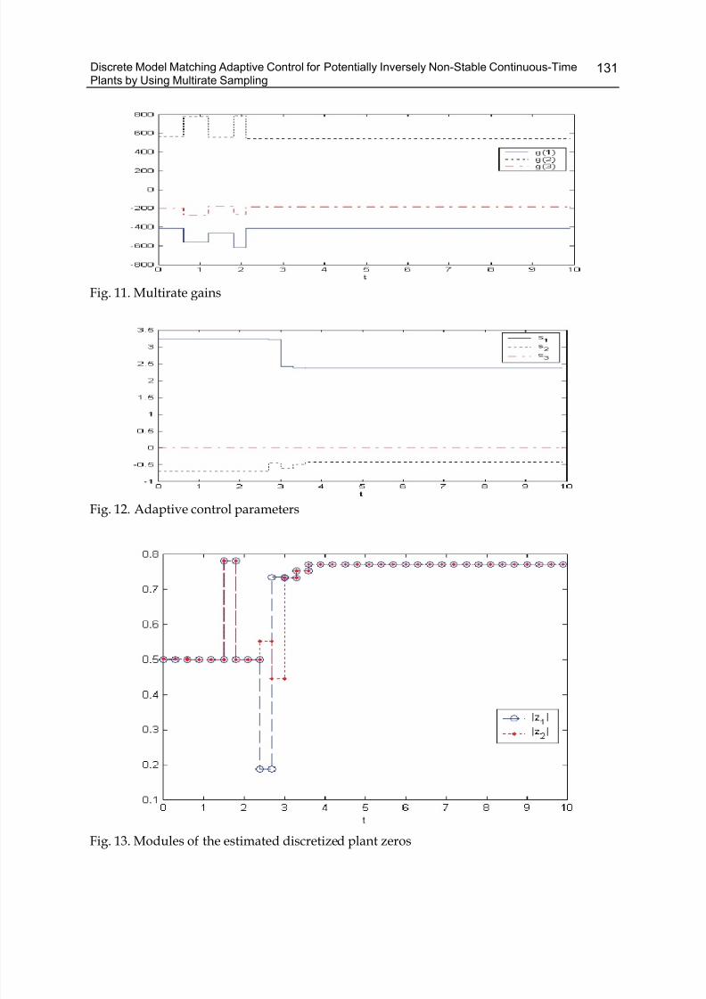
Discrete Model Matching Adaptive Control for Potentially Inversely Non-Stable Continuous-TimePlants by Using Multirate Sampling
131
Fig. 11. Multirate gains
Fig. 12. Adaptive control parameters
Fig. 13. Modules of the estimated discretized plant zeros
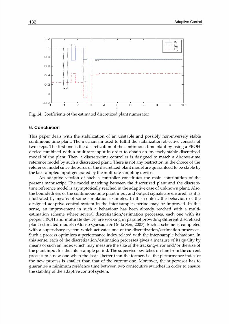
Adaptive Control132
Fig. 14. Coefficients of the estimated discretized plant numerator
6. Conclusion
This paper deals with the stabilization of an unstable and possibly non-inversely stablecontinuous-time plant. The mechanism used to fulfill the stabilization objective consists oftwo steps. The first one is the discretization of the continuous-time plant by using a FROHdevice combined with a multirate input in order to obtain an inversely stable discretizedmodel of the plant. Then, a discrete-time controller is designed to match a discrete-timereference model by such a discretized plant. There is not any restriction in the choice of thereference model since the zeros of the discretized plant model are guaranteed to be stable bythe fast sampled input generated by the multirate sampling device.
An adaptive version of such a controller constitutes the main contribution of thepresent manuscript. The model matching between the discretized plant and the discrete-time reference model is asymptotically reached in the adaptive case of unknown plant. Also,the boundedness of the continuous-time plant input and output signals are ensured, as it isillustrated by means of some simulation examples. In this context, the behaviour of thedesigned adaptive control system in the inter-samples period may be improved. In thissense, an improvement in such a behaviour has been already reached with a multi-estimation scheme where several discretization/estimation processes, each one with itsproper FROH and multirate device, are working in parallel providing different discretizedplant estimated models (Alonso-Quesada & De la Sen, 2007). Such a scheme is completedwith a supervisory system which activates one of the discretization/estimation processes.Such a process optimizes a performance index related with the inter-sample behaviour. Inthis sense, each of the discretization/estimation processes gives a measure of its quality bymeans of such an index which may measure the size of the tracking-error and/or the size ofthe plant input for the inter-sample period. The supervisor switches on-line from the currentprocess to a new one when the last is better than the former, i.e. the performance index ofthe new process is smaller than that of the current one. Moreover, the supervisor has toguarantee a minimum residence time between two consecutive switches in order to ensurethe stability of the adaptive control system.
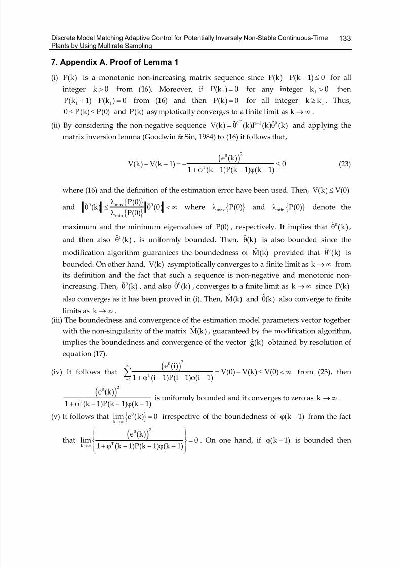
Discrete Model Matching Adaptive Control for Potentially Inversely Non-Stable Continuous-TimePlants by Using Multirate Sampling
133
7. Appendix A. Proof of Lemma 1
(i) P(k) is a monotonic non-increasing matrix sequence since − − ≤P(k) P(k 1) 0 for all
integer >k 0 from (16). Moreover, if =1P(k ) 0 for any integer >1k 0 then
+ − =1 1P(k 1) P(k ) 0 from (16) and then =P(k) 0 for all integer ≥ 1k k . Thus,
≤ ≤0 P(k) P(0) and P(k) asymptotically converges to a finite limit as → ∞k .
(ii) By considering the non-negative sequence −= θ θ% %T0 1 0V(k) (k)P (k) (k) and applying the
matrix inversion lemma (Goodwin & Sin, 1984) to (16) it follows that,
( )− − = − ≤
+ ϕ − − ϕ −
20
T
e (k)V(k) V(k 1) 0
1 (k 1)P(k 1) (k 1)(23)
where (16) and the definition of the estimation error have been used. Then, ≤V(k) V(0)
and
λθ ≤ θ < ∞
λ% %max0 0
min
P(0)(k) (0)
P(0)where λmax P(0) and λmin P(0) denote the
maximum and the minimum eigenvalues of P(0) , respectively. It implies that θ% 0(k ) ,
and then also θ0ˆ (k) , is uniformly bounded. Then, θ(k) is also bounded since the
modification algorithm guarantees the boundedness of M(k) provided that θ0ˆ (k) is
bounded. On other hand, V(k) asymptotically converges to a finite limit as → ∞k from
its definition and the fact that such a sequence is non-negative and monotonic non-
increasing. Then, θ% 0(k) , and also θ0ˆ (k) , converges to a finite limit as → ∞k since P(k)
also converges as it has been proved in (i). Then, M(k) and θ(k) also converge to finite
limits as → ∞k .
(iii) The boundedness and convergence of the estimation model parameters vector together
with the non-singularity of the matrix M(k) , guaranteed by the modification algorithm,
implies the boundedness and convergence of the vector g(k) obtained by resolution of
equation (17).
(iv) It follows that( )
=
= − ≤ < ∞+ ϕ − − ϕ −∑
20k
Ti 1
e (i)V(0) V(k) V(0)
1 (i 1)P(i 1) (i 1)from (23), then
( )+ ϕ − − ϕ −
20
T
e (k)
1 (k 1)P(k 1) (k 1)is uniformly bounded and it converges to zero as → ∞k .
(v) It follows that →∞
=0
klim e (k) 0 irrespective of the boundedness of ϕ −(k 1) from the fact
that( )
→∞
⎧ ⎫⎪ ⎪=⎨ ⎬
+ ϕ − − ϕ −⎪ ⎪⎩ ⎭
20
Tk
e (k)lim 0
1 (k 1)P(k 1) (k 1). On one hand, if ϕ −(k 1) is bounded then
Adaptive Control134
( )→∞
⎧ ⎫⎪ ⎪ =⎨ ⎬+ ϕ − − ϕ −⎪ ⎪⎩ ⎭
20
Tk
e (k)lim 0
1 (k 1)P(k 1) (k 1)implies directly that
→∞=0
klim e (k) 0 . On the other
hand, if ϕ −(k 1) is unbounded then( )
→∞
⎧ ⎫⎪ ⎪ =⎨ ⎬+ ϕ − − ϕ −⎪ ⎪⎩ ⎭
20
Tk
e (k)lim 0
1 (k 1)P(k 1) (k 1)implies that
→∞
⎧ ⎫θ −⎪ ⎪ =⎨ ⎬−⎪ ⎪⎩ ⎭
%2
0
2k
(k 1)lim 0
P(k 1)since = θ − ϕ −% T0 0e (k) (k 1) (k 1) and then →∞
θ − =%2
0
klim (k 1) 0 from
the fact that P(k) is uniformly bounded. Thus, →∞
=0
klim e (k) 0 .
(vi) Provided that the external input sequence c(k) is sufficiently rich such that ϕ −(k 1) is
persistently exciting, θ0ˆ (k) tends to the true parameters vector θ as → ∞k (Goodwin &
Sin, 1984). Then, M(k) tends to 0M (k) from the modification algorithm and,
consequently, θ(k) tends to θ0ˆ (k) and e(k) tends to zero as → ∞k . ***
8. Appendix B. Proof of Theorem 1
(i) Λ(k) is bounded since the estimation model parameters ia (k ) and jb (k) , and the
controller parameters js (k) , for ∈ Ki 1, 2, , n and ∈ +K j 1, 2, , n 1 , are bounded
thanks to the estimated parameters vector θ(k) and the multirate gains vector g(k) are
bounded for all integer ≥k 0 . The eigenvalues of Λ(k) are in <z 1 since they are the
roots of mA (z) and sA (z) , due to the designed control law, and the roots of B(z,k)
which are within the unit circle due to the suitable adaptation of the multirate gains.Besides,
′= +
′ ′Λ − Λ − ≤ γ + γ −∑0
k2
0 1 0k k 1
(k ) (k 1) (k k ) (24)
for all integers k and 0k such that > ≥0k k 0 , and some sufficiently small positive real
constants γ0 and γ1 (Bilbao-Guillerna et al., 2005). Note that (24) is fulfilled with a slow
enough estimation rate via a suitable choice of P(0) in (16) so that γ1 is sufficiently
small. Thus, the time-varying homogeneous system = Λ − −x(k) (k 1) x(k 1) is
exponentially stable and its transition matrix−
′=
′φ = Λ∏k 1
j k
(k,k ) ( j) satisfies ′−′φ ≤ ρ σk k1 0(k ,k )
for all ′≥k k where ( )σ ∈0 0,1 and ρ1 is a non-dependent constant (Alonso-Quesada &
De la Sen, 2004). It follows from (21) that:
Discrete Model Matching Adaptive Control for Potentially Inversely Non-Stable Continuous-TimePlants by Using Multirate Sampling
135
( )′=
′ ′ ′= φ + φ Ψ + Ψ ϑ∑0
k
0 0 1 2k k
x(k) (k,k ) x(k ) (k,k ) e(k ) (k ) (25)
for all integer ≥ ≥0k k 0 . Then,
( )′− −
′=
′ ′= ρ σ + ρ σ ρ + ρ + ρ δ∑0
0
kk k k k
1 0 0 1 0 2 3 4k k
x(k) x(k ) e(k ) (k ) (26)
for some positive real constants ρ2 , ρ3 and ρ4 , provided that the input reference
sequence c(k) is bounded. It follows that→∞
− − =i ik
ˆ ˆlim a (k) a (k 1) 0 and
→∞− − = j j
k
ˆ ˆlim b (k) b (k 1) 0 for all ∈ Ki 1, 2, , n and ∈ +K j 1, 2, , n 1 from the
convergence property of the estimation algorithm. Then,→∞
− − =i ik
ˆ ˆlim s (k) s (k 1) 0 as it
follows from the adaptive control resolution. Consequently,→∞
δ =klim (k) 0 . Besides,
→∞=
klim e(k) 0 from the estimation algorithm. Then, x(k) is bounded from (26), which
implies that sequences u(k) and y(k) are also bounded.
(ii) On one hand, the adaptive control law ensures that the estimated sequence y(k)
matches the reference model one my (k) for all integer ≥k 0 . On the other hand, the
estimation algorithm guarantees the asymptotic convergence of the estimation error
e(k) to zero. Then, the output sequence y(k) tends to my (k) asymptotically as
→ ∞k .
(iii) The adaptive control algorithm ensures that there is no finite escapes. Then, the
boundedness of the sequences u(k) and y(k) implies that the plant input and
output continuous-time signals u(t) and y(t) are bounded for all t.
9. Acknowledgment
The authors are very grateful to MCYT by its partial support through grants DPI 2003-0164and DPI2006-00714.
10. References
Alonso-Quesada, S. & De la Sen, M. (2004). Robust adaptive control of discrete nominallystabilizable plants. Appl. Math. Comput., Vol. 150, pp. 555-583.
Alonso-Quesada, S. & De la Sen, M. (2007). A discrete multi-estimation adaptive controlscheme for stabilizing non-inversely stable continuous-time plants using fractionalholds, Proceedings of 46th IEEE Conference on Decision and Control, pp. 1320-1325,ISBN: 1-4244-1498-9, New Orleans, LA, USA, December 2007, Publisher:Omnipress.
Adaptive Control136
Arvanitis, K. G. (1999). An algorithm for adaptive pole placement control of linear systemsbased on generalized sampled-data hold functions. J. Franklin Inst., Vol. 336, pp.503-521.
Aström, K. J. & Wittenmark, B. (1997). Computer Controlled Systems: Theory and Design,Prentice-Hall Inc., ISBN: 0-13-736787-2, New Jersey.
Bárcena, R., De la Sen, M. and Sagastabeitia, I. (2000). Improving two stability properties ofthe zeros of sampled systems with fractional order hold, IEE Proceedings - ControlTheory and Applications, Vol. 147, No. 4, pp. 456-464.
Bilbao-Guillerna, A., De la Sen, M., Ibeas, A. and Alonso-Quesada, S. (2005). Robustly stablemultiestimation scheme for adaptive control and identification with modelreduction issues. Discrete Dynamics in Nature and Society, Vol. 2005, No. 1, pp. 31-67.
Blachuta, M. J. (1999). On approximate pulse transfer functions. IEEE Transactions on Automatic Control, Vol. 44, No. 11, pp. 2062-2067.
De la Sen, M & Alonso-Quesada, S. (2007). Model matching via multirate sampling with fastsampled input guaranteeing the stability of the plant zeros. Extensions to adaptivecontrol. IET Control Theory Appl., Vol. 1, No. 1, pp. 210-225.
Goodwin, G. C. & Sin, K. S. (1984). Adaptive Filtering, Prediction and Control, Prentice-HallInc., ISBN: 0-13-004069-X, New Jersey.
Goodwin, G. C. & Mayne, D. Q. (1987). A parameter estimation perspective of continuous-time model reference adaptive control. Automatica, Vol. 23, No. 1, pp. 57-70.
Ioannou, P. A. & Sun, J. (1996). Robust Adaptive Control, Prentice-Hall Inc., ISBN: 0-13-439100-4, New Jersey.
Liang, S., Ishitobi M. & Zhu, Q. (2003). Improvement of stability of zeros in discrete-timemultivariable systems using fractional-order hold, International Journal of Control,Vol. 76, No. 17, pp. 1699-1711.
Liang, S. & Ishitobi, M. (2004). Properties of zeros of discretised system using multirateinput and hold, IEE Proc. – Contr. Theory Appl., Vol. 151, No. 2, pp. 180-184.
Narendra, K. S. & Annaswamy, A. M. (1989). Stable Adaptive Systems, Prentice-Hall Inc.,ISBN: 0-13-840034-2, New Jersey.
6
Hybrid Schemes for Adaptive Control Strategies
Ricardo Ribeiro & Kurios QueirozFederal University of Rio Grande do Norte
Brazil
1. Introduction
The purpose of this chapter is to redesign the standard adaptive control schemes by usinghybrid structure composed by Model Reference Adaptive Control (MRAC) or Adaptive PolePlacement Control (APPC) strategies, associated to Variable Structure (VS) schemes forachieving non-standard robust adaptive control strategies. The both control strategies isnow on named VS-MRAC and VS-APPC. We start with the theoretical base of standardcontrol strategies APPC and MRAC, discussing their structures, as how their parameters areidentified by adaptive observers and their robustness properties for guaranteeing theirstability. After that, we introduce the sliding mode control (variable structure) in eachcontrol scheme for simplifying their design procedure. These design procedure are based onstability analysis of each hybrid robust control scheme. With the definition of both hybridcontrol strategies, it is analyzed their behavior when controlling system plants withunmodeled disturbances and parameter variation. It is established how the adaptive lawscompensates these unmodeled dynamics. Furthermore, by using simple systems examples itis realized a comparison study between the hybrid structures VS-APPC and VSMRAC andthe standard schemes APPC and MRAC. As the hybrid structures use switching laws due tothe sliding mode scheme, the effect of chattering is analyzed on the implementation andconsequently effects on the digital control hardware where sampling times are limitingfactor. For reducing these drawbacks it is also discussed possibilities which kind ofmodifications can employ. Finally, some practical considerations are discussed on animplementation on motor drive systems.
2. Variable Structure Model Reference Adaptive Controller (VS-MRAC)
The VS-MRAC was originally proposed in (Hsu et al., 1989) and extensively discussed in(Hsu et al., 1994). The main features of this control scheme are the robustness of parametersuncertainties and unmodeled disturbances, as well as good transitory response.Consider the following first order plant
( )p
p
y
u a
bW s
s =
+= , (1)
Adaptive Control138
where pb and pa are unknown or known with limited uncertainties. Admitting a reference
model given by
( ) m m
m
y
r M
a
bs
s = =
+, (2)
in which 0m k > and 0m a > , the following output error variable can be defined as
0 m e y y = − . (3)
The control objective is to force ( )y t to asymptotically track the reference output signal,
( )m y t , by regulating 0e to be zero, while keeping all the closed-loop signals uniformly
bounded. The control law used for accomplished this is
1 2y u r θ θ+= , (4)
which is the same as used in traditional model reference adaptive control. However, insteadof the integral adaptive laws for the controller parameters, switching laws are proposed inorder to improve the system transient performance and its robustness.
If pb and pa are known, the ideal controller parameters ( *1θ and *
2θ ) can be founded using
the following condition
m y y
r r = , (5)
which means that our control objective is achieved, i.e., the closed-loop system behaves likethe open-loop reference model. Consequently, the control law equation can be rewritten as
* *21y u r θ θ+= . (6)
Analyzing (1) and (2) in the time domain, we get
p py a y k u = − + , (7)
m m m m y a y r k = − + . (8)
Adding and subtracting terms related to the ideal control parameters in (4),
* * * *1 2 1 2 1 2y r y r y r u θ θ θ θ θ θ+ − − + += , (9)
Hybrid Schemes for Adaptive Control Strategies 139
and then grouping some terms
* * * *1 1 2 2 1 2( ) ( )y u r y r θ θ θ θ θ θ− + − + += , (10)
we have
* *1 2 1 2y r y r u θ θ θ θ+ + += , (11)
in which terms 1θ and 2θ
are deviations of ideal controller parameters 1θ and 2θ .
Substituting the resulting equation (11) in (7),
* *1 2 1 2( )p pa y y b y r y r θ θ θ θ+ + + += − , (12)
we can rewrite this equation as
* *1 2 1 2( )p p p pa y b y y b r b y r θ θ θ θ= − + ++ + , (13)
which results in
* *1 2 1 2) (( )p p p pa by y b r b y r θ θ θ θ+ + += − − . (14)
From (6), the model input r can be defined as
*1
*2
y r
u θ
θ=
−. (15)
Therefore, using (11) and (15) in (8), we get
1 2*2
( )m m m m y a y b r y r
bθ θ
θ= − + + + . (16)
Finally, comparing (14) and (16) due to the condition (5), we have the desired controllerparameters
*1
p m
p
a
b
a θ
−= , (17)
Adaptive Control140
*2
m
p
b
bθ = . (18)
The above desired controller parameters assure that plant output converges to its reference
model, becausepb and
pa are known. This design criteria is named as The Matching
Conditions.However, our interests are concerned with unknown plant parameters or with known plantparameters with uncertainties, which require the use of adaptive laws for adjustingcontroller parameters. Derivating the output error equation given in (3),
0 m e y y = − (19)
and using the condition (5), with equations (8), (16) and (19), we get
0 1 2*2
( ) ( )m m m m m m
be a y b r y r a y b r θ θ
θ= − + + + − − + , (20)
which can be rearranged as
0 1 2*2
)) (( m m m e a
by y y r θ θ
θ= − + +− . (21)
Thus,
0 0 1 2*2
( )m m e a e y r
bθ θ
θ= − + + . (22)
Now, consider the Lyapunov function candidate given by
20 0
1( 0)
2V e e >= , (23)
and its respective first time derivative
0 0 0( )V e e e = . (24)
By substituting (22) in (24), we obtain the following equation
Hybrid Schemes for Adaptive Control Strategies 141
0 0 1 2 0*2
( ) ( )m m V e a e r
by e θ θ
θ
⎡ ⎤⎢ ⎥= − + +⎢ ⎥⎢ ⎥⎣ ⎦
, (25)
that can be rewritten as
( ) ( )2 * *0 0 1 1 0 2 2 0*
2
( ) m m V e e e y e r
ba θ θ θ θ
θ= − ⎡ ⎤+ − + −⎢ ⎥⎣ ⎦
. (26)
Using the switching laws,
1 1 0( )sgn e y θ θ= − , (27)
2 2 0( )sgn e r θ θ= − , (28)
we obtain,
( ) ( )2 * *0 0 1 0 1 0 2 0 2 0*
2
| |( ) | |m m V e e y e y
br a r e e e θ θ θ θ
θ= − ⎡ ⎤+ + +⎢ ⎥⎣
−⎦
. (29)
If the conditions *1 1| |θ θ> and 2 2
*| |θ θ> are satisfied, the terms with indefinite signals
in (29) are dominated, and then
20 0( ) 0m V e a e −≤ < (30)
which guarantees that 0 0e = is a globally asymptotically stable (GAS) equilibrium point,
because (30) is a negative definite function.
3. Variable Structure Adaptive Pole Placement Control (VS-APPC)
As the VS-MRAC, the VS-APPC is the hybrid control structure obtained from theassociation of Pole Placement Control (PPC) together with Variable Structure (VS).Therefore, the theoretical development of this section starts from PPC control scheme andthen we introduce the VS concepts for achieving the proposed VS-APPC.
Considering the single input/single output (SISO) LTI plant
( )y G s u = , (31)
in which
Adaptive Control142
11 1 0
11 1 0
...( )( )
( ) ...
n n
n n n
b s b s bZ s G s
R s s a s a s a
−−
−−
+ + += =
+ + + + , (32)
there are, as plant parameters, 2n elements, which are the coefficients of the numerator and
denominator of transfer function ( )G s . We can define the vector *θ as
*1 1 0 1 1 0. . . . . .
T
n n b b b a a a θ − −⎡ ⎤= ⎢ ⎥⎣ ⎦
. (33)
From this, the following constraints must be observed:
S1. ( )R s is a monic polynomial whose degree n is known.
S2. ( )Z s , ( )R s are coprime and degree( )Z n < .
Assumptions (S1) and (S2) allow ( )Z s , ( )R s to be non-Hurwitz in contrast to the MRC
(Model Reference Control) case, where ( )Z s is required to be Hurwitz.
We can also extend the PPC scheme for including the tracking objective, where output y is
required to follow a certain class of reference signals r , by using the internal modelprinciple (Ioannou & Sun, 1996). The uniformly bounded reference signal is assumed tosatisfy
( ) 0m Q s r = , (34)
where ( )m Q s , the internal model of r , is a known monic polynomial of degree q with non-
repeated roots on the jω -axis and satisfies
S3. ( )m Q s , ( )Z s are coprime.
Considering the control law given by
( ) ( ) ( ) ( )m Q s L s u P s y M s r = − + , (35)
where ( )P s , ( )M s , ( )L s are polynomials (with ( )L s monic) of degree – 1q n + ,
– 1q n + e – 1n , respectively, and ( )m Q s satisfies (34) and assumption (S3).
Applying (35) to the plant (31), we obtain the closed-loop plant equation
( ) ( )
( ) ( ) ( ) ( ) ( )m
Z s M s y r
Q s L s R s P s Z s =
+, (36)
whose characteristic equation is
Hybrid Schemes for Adaptive Control Strategies 143
( ) ( ) ( ) ( ) ( ) 0m Q s L s R s P s Z s + = , (37)
and has order 2 1n q + − . The objective now is chosen ( )P s , ( )L s such that
*( ) ( ) ( ) ( ) ( ) ( )m Q s L s R s P s Z s A s + = (38)
is satisfied for a given monic Hurwitz polynomial *( )A s of degree 2 1n q + − . Because of
assumptions S2 e S3 which guarantee that ( )m Q s , ( )R s , ( )Z s are coprime, there is a
solution so that ( )L s and ( )P s satisfy (38) and this solution is unique (Ioannou & Sun,
1996).
Using (38), the closed-loop is described by
*
( ) ( )
( )
Z s M s y r
A s = . (39)
Similarly, from the plant (31) and the control law (35) and (38), we obtain
*
( ) ( )
( )
R s M s u r
A s = . (40)
Because r is uniformly bounded and*
( ) ( )
( )
Z s M s
A s ,
*
( ) ( )
( )
R s M s
A s are proper with stable poles,
y and u remain bounded whenever t →∞ for any polynomial ( )M s of degree
– 1n q + (Ioannou & Sun, 1996). Therefore, the pole placement objective is achieved by
the control law (35) without having any additional restrictions in ( )M s and ( )m Q s . When
0r = , (39) and (40) imply that y and u converge to zero exponentially fast. On the other
hand, when 0r ≠ , the tracking error e y r = − is given by
*
* * *
( ) ( ) ( ) ( ) ( ) ( )[ ( ) ( )] ( )
( ) ( ) ( )m
Z s M s A s Z s L s R s e r M s P s r Q s r
A s A s A s
−= = − − . (41)
In order to obtain zero tracking error, the equation above suggests the choice of
( ) ( )M s P s = to cancel its first term, while the second term can be canceled by using (34).
Therefore, the pole placement and tracking objective are achieved by using the control law
( ) ( ) ( )( )m Q s L s u P s y r = − − , (42)
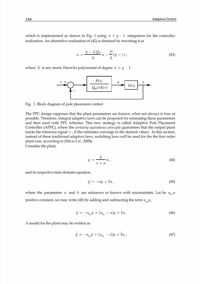
Adaptive Control144
which is implemented as shown in Fig. 1 using – 1n q + integrators for the controller
realization. An alternative realization of (42) is obtained by rewriting it as
( )m LQ P
u u y r Λ −
= − −Λ Λ
, (43)
where Λ is any monic Hurwitz polynomial of degree – 1n q + .
G(s)Qm(s)L(s)
P(s)r u y+
−
Fig. 1. Block diagram of pole placement control.
The PPC design supposes that the plant parameters are known, what not always is true orpossible. Therefore, integral adaptive laws can be proposed for estimating these parametersand then used with PPC schemes. This new strategy is called Adaptive Pole PlacementController (APPC), where the certainty equivalence principle guarantees that the output planttracks the reference signal r , if the estimates converge to the desired values. In this section,instead of these traditional adaptive laws, switching laws will be used for the the first orderplant case, according to (Silva et al., 2004).
Consider the plant,
by u
s a =
+, (44)
and its respective time domain equation,
a y y bu = − + , (45)
where the parameters a and b are unknown or known with uncertainties. Let be m a a
positive constant, we may write (45) by adding and subtracting the term m a y ,
( )m m a y a a y y bu = − + − + . (46)
A model for the plant may be written as
ˆ ˆˆ ˆ( )m m a y a y a y bu = − + − + , (47)
Hybrid Schemes for Adaptive Control Strategies 145
where a and b are estimates for a and b , respectively (Ioannou & Sun, 1996).
We define the estimation error 0e as
0 ˆe y y = − , (48)
and with (46) and (47), we get
00 m a e ay bu e = − + − , (49)
where
ˆa a a = − , (50)
ˆb b b= − . (51)
Choosing the following Lyapunov function candidate,
20 0
1( ) 0
2V e e = > , (52)
we have
0 0 0( )V e e e = , (53)
which can be rewritten using (49),
20 0 00)( m a e ae y be u V e = − + − . (54)
Expanding the above equation with (50) and (51),
20 0 00
ˆˆ( ) (( ) )m a e a V a e y b e u e b= − + − − − , (55)
and then using the switching laws,
0ˆ sgn( )a a e y = − , (56)
0ˆ sgn( )b b e u = , (57)
we get,
Adaptive Control146
20 0 0 00 0( ) (( ) )m a e a e y ae y b e u be V e u = − − + − − . (58)
Finally, if the conditions a a > and b b> are satisfied,
02
0) 0( m V e a e ≤ − < , (59)
which guarantees that 0 0e = is a globally asymptotic stable (GAS) equilibrium point.
Moreover, if we follow a similar procedure described in (Hsu & Costa, 1989), we can prove
that 0 0e = reaches the sliding surface in a finite time f t ( 0 0e = , f t t ∀ > ).
4. Application on a Current Control Loop of an Induction Machine
To evaluate the performance of both proposed hybrid adaptive schemes, we use aninduction machine voltage x current model as an experimental plant. The voltage equationsof the induction machine on arbitrary reference frame can be presented by the followingequations:
g g g g s s sd g s s g rd sd s sd s g s sq r rq
r m r
l l di l l v r i l l i
dt l
σ σ φσ ω σ ω φ
τ τ
⎛ ⎞⎛ ⎞ ⎛ ⎞− − ⎟⎜⎟ ⎟⎜ ⎜ ⎟⎜⎟ ⎟= + + − − +⎜ ⎜ ⎟⎟ ⎟⎜⎜ ⎜ ⎟⎟ ⎟⎜ ⎜ ⎜ ⎟⎜⎝ ⎠ ⎝ ⎠⎝ ⎠ , (60)
g g sq rq g g g s s g s s
sq s sq s g s sd r rd r m r
di l l l l v r i l l i
dt l
φσ σσ ω σ ω φ
τ τ
⎛ ⎞⎛ ⎞ ⎛ ⎞− − ⎟⎜⎟ ⎟⎜ ⎜ ⎟⎜⎟ ⎟= + + + + − ⎟⎜ ⎜ ⎜⎟ ⎟ ⎟⎜ ⎜ ⎜⎟ ⎟⎜ ⎜ ⎟⎝ ⎠ ⎝ ⎠ ⎟⎜⎝ ⎠ , (61)
where g sd v , g
sq v , g sd i and g
sq i are dq axis stator voltages and currents in a generic reference
frame, respectively; s r , s l and m l are the stator resistance, stator inductance and mutual
inductance, respectively; g ω and r ω are the angular frequencies of the dq generic reference
frame and rotor reference frame, respectively; 2 /1 m s r l l l σ = − and /r r r l r τ = are the
leakage factor and rotor time constant, respectively.
The above model can be simplified by choosing the stator reference frame ( 0g ω = ).
Therefore, equations (60) and (61) can be rewritten as
s s s sd s sd sr sd s sd
di v r i l e
dt σ= + + , (62)
Hybrid Schemes for Adaptive Control Strategies 147
s sq s s s
sq sr sq s sq
di v r i l e
dt σ= + + , (63)
where s is the superscript related to the stator reference frame, ( ) /sr s s s r r r l l σ τ = + − ,
s sd e and s
sq e are fcems of the dq machine phases given by
( )s s s rd s s sd r rq
r m
l l e
l
φ σω φ
τ
⎛ ⎞ −⎟⎜ ⎟⎜= − + ⎟⎜ ⎟⎜ ⎟⎝ ⎠, (64)
and
( )s rq s s s s
sq r rd r m
l l e
l
φ σω φ
τ
⎛ ⎞ −⎟⎜ ⎟⎜= − ⎟⎜ ⎟⎜ ⎟⎟⎜⎝ ⎠, (65)
The current x voltage transfer function of the induction machine can be obtained from (62)and (63) as
( ) ( ) 1 /
1( ) ( )
s s sd sd sr
s s s sd sd
I s I s r
s V s V s τ ′ ′= =
+, (66)
where /s s sr l r τ σ= , ( ) ( ) ( )s s s sd sd sd V s V s E s ′ = − and '( ) ( ) ( )s s s
sq sq sq V s V s E s = − . The fcems
( )s sd E s and ( )s
sq E s are considered unmodeled disturbances to be compensated by the
control scheme.Analyzing the current x voltage transfer functions of a standard machine, we can observe
that the time constants τ has parameters which vary with the dynamic behavior of
machine. Moreover, this plant has also unmodeled disturbances. This justifies the use of thiscontrol plant for evaluating the performance of proposed control schemes.
5. Control System
Fig. 2 presents the block diagram of a standard vector control strategy, in which theproposed control schemes are employed for induction motor drive. Block RFO realizes the
vector rotor field oriented control strategy. It generates the stator reference currents s sd i ∗ and
s sq i ∗ , angular stator frequency o ω∗ of stator reference currents from desired reference torque
e T ∗ , and reference rotor flux r φ∗ , respectively. Blocks VS-ACS implement the proposed
robust adaptive current control schemes that could be the VS-MRAC strategy or the VS-
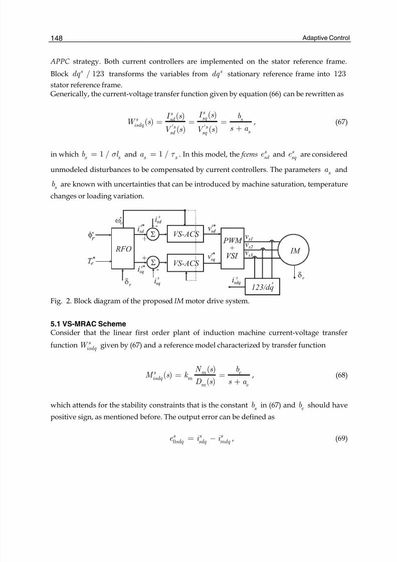
Adaptive Control148
APPC strategy. Both current controllers are implemented on the stator reference frame.
Block / 123s dq transforms the variables from s dq stationary reference frame into 123
stator reference frame. Generically, the current-voltage transfer function given by equation (66) can be rewritten as
( )( )( )
( ) ( )
s s sq s sd s
isdq s s s sd sq
I s I s bW s
s a V s V s ′ ′= = =
+, (67)
in which 1 /s s b l σ= and 1 /
s s a τ = . In this model, the fcems s sd e and s
sq e are considered
unmodeled disturbances to be compensated by current controllers. The parameters s a and
s b are known with uncertainties that can be introduced by machine saturation, temperature
changes or loading variation.
123/dq s
s
IM
s
s
s
s
s
RFO
s
fr *
wo*
VS-ACS
VS-ACS
Fig. 2. Block diagram of the proposed IM motor drive system.
5.1 VS-MRAC SchemeConsider that the linear first order plant of induction machine current-voltage transfer
function s isdq W given by (67) and a reference model characterized by transfer function
( )( )
( )s m e isdq m
m e
N s bM s k
D s s a = =
+, (68)
which attends for the stability constraints that is the constants
b in (67) ande
b should have
positive sign, as mentioned before. The output error can be defined as
0s s s
sdq sdq mdq e i i = − , (69)
Hybrid Schemes for Adaptive Control Strategies 149
where s mdq i ( s
md i and s mq i ) are the outputs of the reference model. The tracking of the model
control signal ( s s sd md i i = or s s
sq mq i i = ) is reached if the input of the control plant is defined
as
1 2 s s s sdq dq sdq dq sdq v i i θ θ∗ ∗ ∗= + (70)
where 1d θ∗ ( 1q θ∗ ) and 2d θ∗ ( 2q θ∗ ) are the ideal controller parameters, that can be only
determined if ( )s isdq W s is known. According to section 2, they can be determined as
1 1s e
d q s
a a
bθ θ∗ ∗ −
= = , (71)
and
2 2e
d q
s
b
bθ θ∗ ∗= = . (72)
Once ( )s isdq W s is not known, the controllers parameters 1 ( )dq t θ and 2 ( )dq t θ are updated by
using switching laws as
0( )s s idq idq sdq isdq
sgn e y θ θ= − (73)
where [1,2]i = and s sdq
y is the reference currents s sdq
i ∗ or the output currents s sdq
i , and
idq idq θ θ∗> are upper bounds which are assumed to be known, and the signal-function
sgn is defined as
1 0( )
1 0
if x sgn x
if x
⎧ >⎪⎪= ⎨⎪− <⎪⎩
. (74)
Introducing nominal values of controller parameters ( )idq nom θ (ideally ( )idq nom idq θ θ∗= ). It is
convenient to modify the control plant input given by (70) for the following
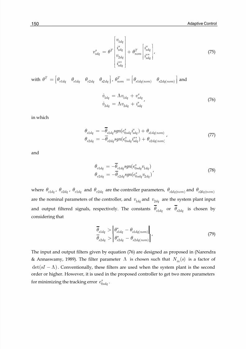
Adaptive Control150
1
2
dq
s s sdq sdq s T T
sdq nom s dq sdq
s sdq
v
i i v
v i
i
θ θ∗
∗
⎡ ⎤⎢ ⎥⎢ ⎥ ⎡ ⎤⎢ ⎥ ⎢ ⎥= +⎢ ⎥ ⎢ ⎥⎢ ⎥ ⎢ ⎥⎣ ⎦⎢ ⎥⎢ ⎥⎣ ⎦
, (75)
with 1 1 2 2T
v dq s dq v dq s dq θ θ θ θ θ⎡ ⎤= ⎢ ⎥⎣ ⎦, 1 ( ) 2 ( )
T nom s dq nom s dq nom θ θ θ⎡ ⎤= ⎢ ⎥⎣ ⎦
and
1 1
2 2
s dq dq sdq
s dq dq sdq v
v v
v i
v = Λ +
= Λ +
, (76)
in which
1 1 0 1 ( )
2 2 0 2 ( )
( )
( )
s s s dq s dq sdq sdq s dq nom
s s s dq s dq sdq sdq s dq nom
sgn e i
sgn e i
θ θ θ
θ θ θ∗
= − +
= − +, (77)
and
1 1 0 1
2 2 0 2
( )
( )
s v dq v dq sdq dq
s v dq v dq sdq dq
sgn e v
sgn e v
θ θ
θ θ
= −
= −, (78)
where 1s dq θ , 2s dq θ , 1v dq θ and 2v dq θ are the controller parameters, 1 ( )s dq nom θ and 2 ( )s dq nom θ
are the nominal parameters of the controller, and 1dq v and 2dq v are the system plant input
and output filtered signals, respectively. The constants 1s dq θ or 2s dq θ is chosen by
considering that
1 1 1 ( )
2 2 2 ( )
s dq s dq s dq nom
s dq s dq s dq nom
θ θ θ
θ θ θ
∗
∗
> −
> −, (79)
The input and output filters given by equation (76) are designed as proposed in (Narendra
& Annaswamy, 1989). The filter parameter Λ is chosen such that ( )m N s is a factor of
det( )sI − Λ . Conventionally, these filters are used when the system plant is the second
order or higher. However, it is used in the proposed controller to get two more parameters
for minimizing the tracking error 0s
sdq e .
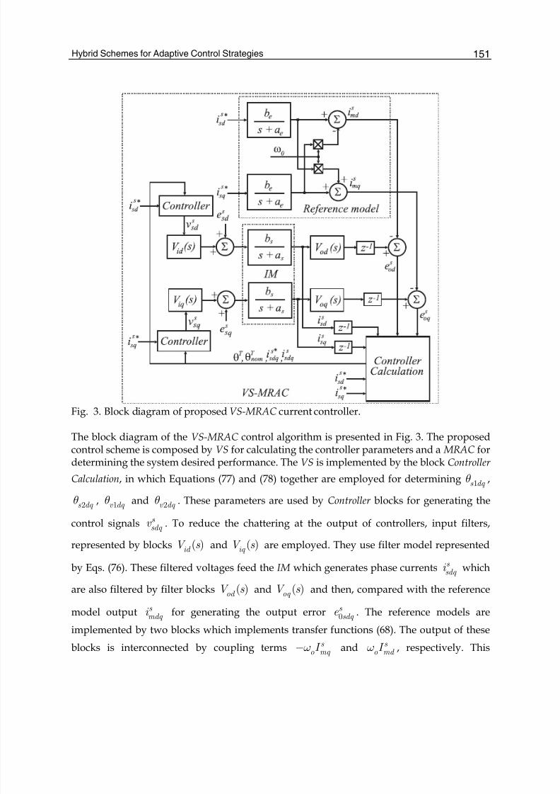
Hybrid Schemes for Adaptive Control Strategies 151
Fig. 3. Block diagram of proposed VS-MRAC current controller.
The block diagram of the VS-MRAC control algorithm is presented in Fig. 3. The proposedcontrol scheme is composed by VS for calculating the controller parameters and a MRAC fordetermining the system desired performance. The VS is implemented by the block Controller
Calculation, in which Equations (77) and (78) together are employed for determining 1s dq θ ,
2s dq θ , 1v dq θ and 2v dq θ . These parameters are used by Controller blocks for generating the
control signals s sdq v . To reduce the chattering at the output of controllers, input filters,
represented by blocks ( )id V s and ( )iq V s are employed. They use filter model represented
by Eqs. (76). These filtered voltages feed the IM which generates phase currents s sdq i which
are also filtered by filter blocks ( )od V s and ( )oq V s and then, compared with the reference
model output s mdq i for generating the output error 0
s sdq e . The reference models are
implemented by two blocks which implements transfer functions (68). The output of these
blocks is interconnected by coupling terms s o mq I ω− and s
o md I ω , respectively. This
Adaptive Control152
approach used to avoid the phase delay between the input ( s sdq I ∗ ) and output ( s
mdq I ∗ ) of the
reference model.
5.1.1 Design of the ControllerTo design the proposed VS-MRAC controller, initially is necessary to choose a suitable
reference model ( )s isdq M s . Based on the parameters of the induction machine used in
present study, given in Table 1, the reference model employed is
550( )
550s isdq M s
s =
+, (80)
From this reference model, the nominal values can be determined by using equations (71)
and (72) which results in 1 ( ) 1 ( ) 3.7sd nom sq nom θ θ= = and 2 ( ) 2 ( ) 55sd nom sq nom θ θ= = .
Considering the restrictions given by (79), the parameters 1s dq θ and 2s dq θ , chosen for
achieving a control signal with minimum amplitude are 1 0.37s dq θ = and 2 5.5s dq θ = . It
is important to highlight that choice criteria determines how fast the system converges totheir references. Moreover, it also determines the level of the chattering verified at thecontrol system after its convergence. As mentioned before the use of input and output filtersare not required for control plant of fist order. They are used here for smoothing the controlsignal. Their parameters was determined experimentally, which results in
1Λ = , 1 1 2.0v d v d θ θ= = and 2 2 0.1v d v q θ θ= = . This solution is not unique and
different adjust can be employed on these filters setup which addresses to different overallsystem performance.
5.2 VS-APPC SchemeThe first approach of VS-APPC in (Silva et al., 2004) does not deal with unmodeleddisturbances occurred at the system control loop like machine fems. To overcome this, amodified VS-APPC is proposed here.Let us consider the first order IM current-voltage transfer function given by equation (67).
The main objective is to estimate parameters s a and s b to generate the inputs sd v and sq v
so that the machine phase currents s sd i and s
sq i following their respective reference currents
s sd i ∗ and s
sd i ∗ and, the closed loop poles are assigned to those of a Hurwitz polynomials
( )s A s ∗ given by
3 22 1 0( )A s s s s α α α∗ ∗ ∗ ∗= + + + , (81)
Hybrid Schemes for Adaptive Control Strategies 153
where coefficients 2α∗ , 1α
∗ and 0α∗ determine the closed-loop performance requirements.
To estimate the parameters s a and s b , the respective switching laws are used
0ˆ ( )s s s s sdq sdq a a sgn e i = − , (82)
0ˆ ( )s s s s sdq sdq b b sgn e v = , (83)
with the restrictions s s a a > and s s b b> satisfied, as mentioned before. The pole
placements and the tracking objectives of proposed VS-APPC are achieved, if the followingcontrol law is employed
( ) ( ) ( ) ( )( )s s s m sdq sdq sdq Q s L s V s P s I I ∗= − − (84)
which addresses to the implementation of the controller transfer function
( )( ) ( )
( ) ( )sd sq m
P s C s C s
Q s L s = = . (85)
The polynomial ( )m Q s is choose to satisfy ( ) ( ) ( ) ( ) 0s s m sd m sq Q s I s Q s I s ∗ ∗= = . For the IM
current-voltage control plant (see equation (67)) and considering that the VS-APPC controlalgorithms are implemented on the stator reference frame, which results in sinusoidal
reference currents, a suitable choice for the controller polynomials are 2 2( )m o Q s s ω∗= +
(internal model of sinusoidal reference signals sd i ∗ and sq i ∗ ), ( ) 1L s = and
22 1 0ˆ ˆ ˆ( )P s p s p s p= + + , where o ω∗ is the angular frequency of reference currents. This
choice results in a current controller with the following transfer functions
22 1 0
2 2
ˆ ˆ ˆ( ) ( ) sd sq
o
p s p s pC s C s
s ω∗
+ += =
+(86)
where angular frequency o ω∗ is generated by vector RFO control scheme and coefficients 2p ,
1p and 0p are determined by solving the Diophantine equation for desired Hurwitz
polynomial s A∗ (see equation (81)) as follows
22
ˆˆ
ˆs
s
a p
b
α∗ −= (87)
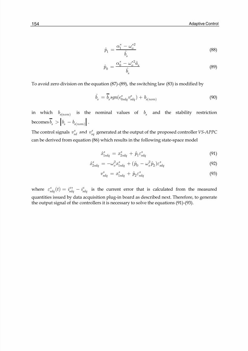
Adaptive Control154
21
1 ˆ ˆ
o
s
pb
α ω∗ ∗−= (88)
20
0 ˆ
ˆo s
s
a p
b
α ω∗ ∗−= (89)
To avoid zero division on the equation (87)-(89), the switching law (83) is modified by
0 ( )ˆ ( )s s s s sdq sdq s nom b b sgn e v b= + (90)
in which ( )s nom b is the nominal values of s b and the stability restriction
becomes ( )s s s nom b b b> − .
The control signals s sd v and s
sq v generated at the output of the proposed controller VS-APPC
can be derived from equation (86) which results in the following state-space model
1 2 1s s s sdq sdq sdq x x p ε= + (91)
2 22 1 0 2ˆ ˆ( )s s s
sdq o sdq o sdq x x p pω ω ε= − + − (92)
1 2s s s sdq sdq sdq v x p ε= + (93)
where ( )s s s sdq sdq sdq t i i ε ∗= − is the current error that is calculated from the measured
quantities issued by data acquisition plug-in board as described next. Therefore, to generatethe output signal of the controllers it is necessary to solve the equations (91)-(93).
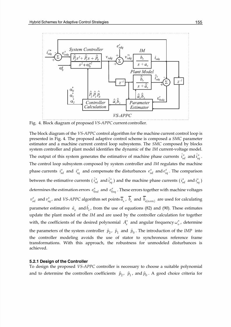
Hybrid Schemes for Adaptive Control Strategies 155
Fig. 4. Block diagram of proposed VS-APPC current controller.
The block diagram of the VS-APPC control algorithm for the machine current control loop ispresented in Fig. 4. The proposed adaptive control scheme is composed a SMC parameterestimator and a machine current control loop subsystems. The SMC composed by blockssystem controller and plant model identifies the dynamic of the IM current-voltage model.
The output of this system generates the estimative of machine phase currents s sd i and s
sq i .
The control loop subsystem composed by system controller and IM regulates the machine
phase currents s sd i and s
sq i and compensate the disturbances s sd e and s
sq e . The comparison
between the estimative currents ( s sd i and s
sq i ) and the machine phase currents ( s sd i and s
sq i )
determines the estimation errors 0s
sd e and 0s
sq e . These errors together with machine voltages
s sd v and s
sq v , and VS-APPC algorithm set pointss a ,
s b and ( )s nom b are used for calculating
parameter estimative s a and ˆs b , from the use of equations (82) and (90). These estimates
update the plant model of the IM and are used by the controller calculation for together
with, the coefficients of the desired polynomial s A∗ and angular frequency o ω∗ , determine
the parameters of the system controller 2p , 1p and 0p . The introduction of the IMP into
the controller modeling avoids the use of stator to synchronous reference frametransformations. With this approach, the robustness for unmodeled disturbances isachieved.
5.2.1 Design of the ControllerTo design the proposed VS-APPC controller is necessary to choose a suitable polynomial
and to determine the controllers coefficients 2p , 1p , and 0p . A good choice criteria for
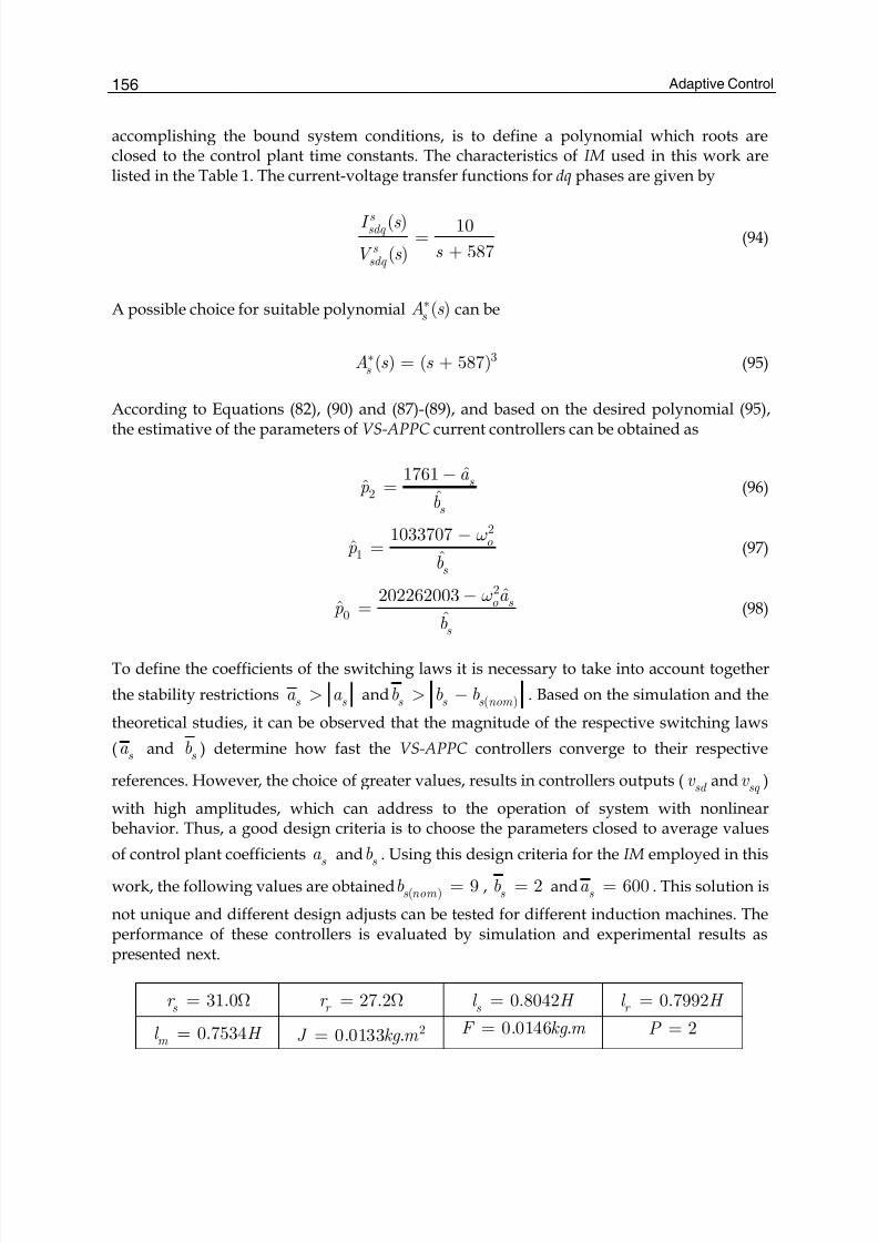
Adaptive Control156
accomplishing the bound system conditions, is to define a polynomial which roots areclosed to the control plant time constants. The characteristics of IM used in this work arelisted in the Table 1. The current-voltage transfer functions for dq phases are given by
( ) 10
587( )
s sdq
s sdq
I s
s V s =
+(94)
A possible choice for suitable polynomial ( )s A s ∗ can be
3( ) ( 587) s A s s ∗ = + (95)
According to Equations (82), (90) and (87)-(89), and based on the desired polynomial (95),the estimative of the parameters of VS-APPC current controllers can be obtained as
2
ˆ1761ˆ
ˆs
s
a p
b
−= (96)
2
1
1033707ˆ
ˆo
s
pb
ω−= (97)
2
0
ˆ202262003ˆ
ˆo s
s
a p
b
ω−= (98)
To define the coefficients of the switching laws it is necessary to take into account together
the stability restrictionss s a a > and ( )s s s nom b b b> − . Based on the simulation and the
theoretical studies, it can be observed that the magnitude of the respective switching laws
( s a and s b ) determine how fast the VS-APPC controllers converge to their respective
references. However, the choice of greater values, results in controllers outputs ( sd v and sq v )
with high amplitudes, which can address to the operation of system with nonlinearbehavior. Thus, a good design criteria is to choose the parameters closed to average values
of control plant coefficients s a and s b . Using this design criteria for the IM employed in this
work, the following values are obtained ( ) 9s nom b = , 2s b = and 600s a = . This solution is
not unique and different design adjusts can be tested for different induction machines. Theperformance of these controllers is evaluated by simulation and experimental results aspresented next.
31.0s r = Ω 27.2r r = Ω 0.8042s l H = 0.7992r l H =
0.7534m l H = 20.0133 .J kg m = 0.0146 .F kg m = 2P =
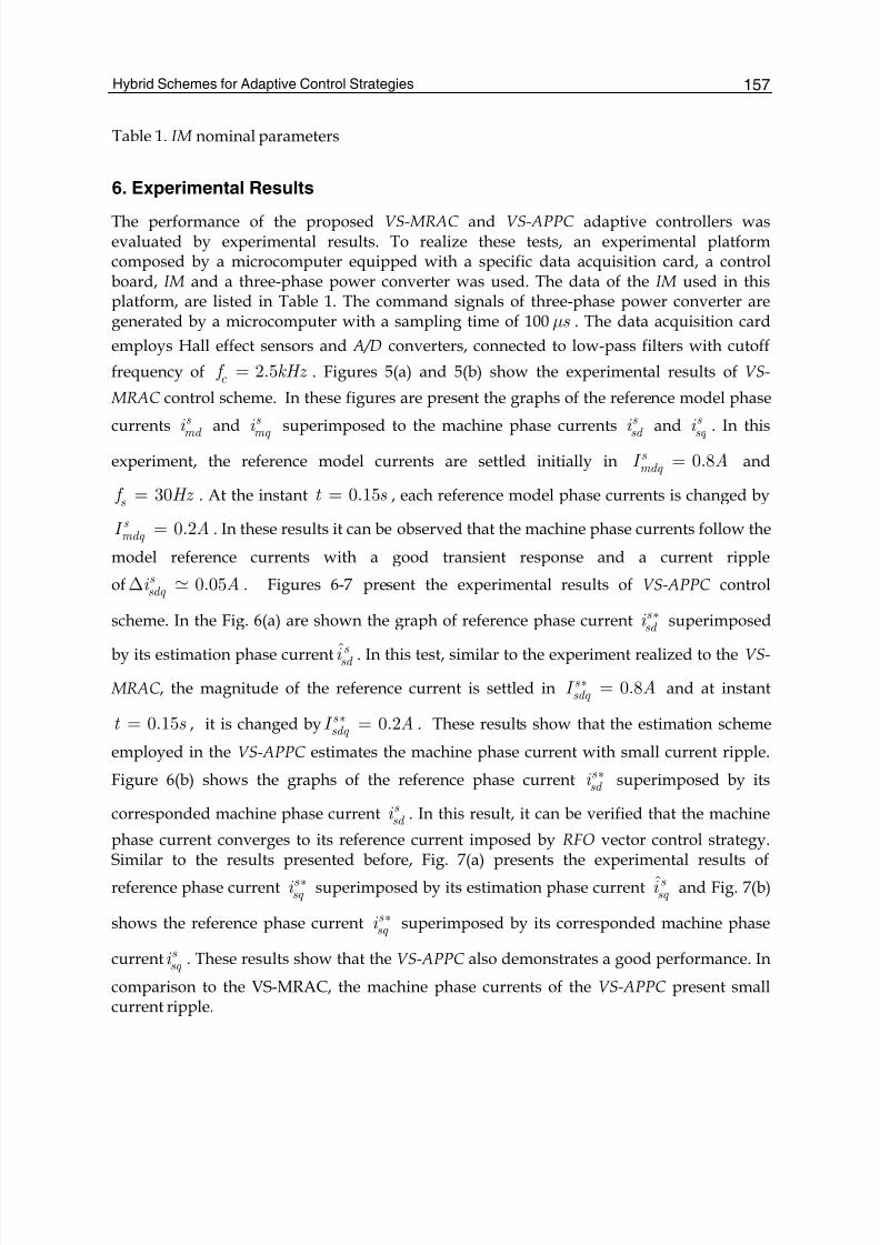
Hybrid Schemes for Adaptive Control Strategies 157
Table 1. IM nominal parameters
6. Experimental Results
The performance of the proposed VS-MRAC and VS-APPC adaptive controllers wasevaluated by experimental results. To realize these tests, an experimental platformcomposed by a microcomputer equipped with a specific data acquisition card, a controlboard, IM and a three-phase power converter was used. The data of the IM used in thisplatform, are listed in Table 1. The command signals of three-phase power converter aregenerated by a microcomputer with a sampling time of 100 s μ . The data acquisition card
employs Hall effect sensors and A/D converters, connected to low-pass filters with cutoff
frequency of 2.5c f kHz = . Figures 5(a) and 5(b) show the experimental results of VS-
MRAC control scheme. In these figures are present the graphs of the reference model phase
currents s md i and s
mq i superimposed to the machine phase currents s sd i and s
sq i . In this
experiment, the reference model currents are settled initially in 0.8s mdq I A= and
30s f Hz = . At the instant 0.15t s = , each reference model phase currents is changed by
0.2s mdq I A= . In these results it can be observed that the machine phase currents follow the
model reference currents with a good transient response and a current ripple
of 0.05s sdq i AΔ . Figures 6-7 present the experimental results of VS-APPC control
scheme. In the Fig. 6(a) are shown the graph of reference phase current s sd i ∗ superimposed
by its estimation phase current s sd i . In this test, similar to the experiment realized to the VS-
MRAC , the magnitude of the reference current is settled in 0.8s sdq I A∗ = and at instant
0.15t s = , it is changed by 0.2s sdq I A∗ = . These results show that the estimation scheme
employed in the VS-APPC estimates the machine phase current with small current ripple.
Figure 6(b) shows the graphs of the reference phase current s sd i ∗ superimposed by its
corresponded machine phase current s sd i . In this result, it can be verified that the machine
phase current converges to its reference current imposed by RFO vector control strategy.Similar to the results presented before, Fig. 7(a) presents the experimental results of
reference phase current s sq i ∗ superimposed by its estimation phase current s
sq i and Fig. 7(b)
shows the reference phase current s sq i ∗ superimposed by its corresponded machine phase
current s sq i . These results show that the VS-APPC also demonstrates a good performance. In
comparison to the VS-MRAC, the machine phase currents of the VS-APPC present smallcurrent ripple.
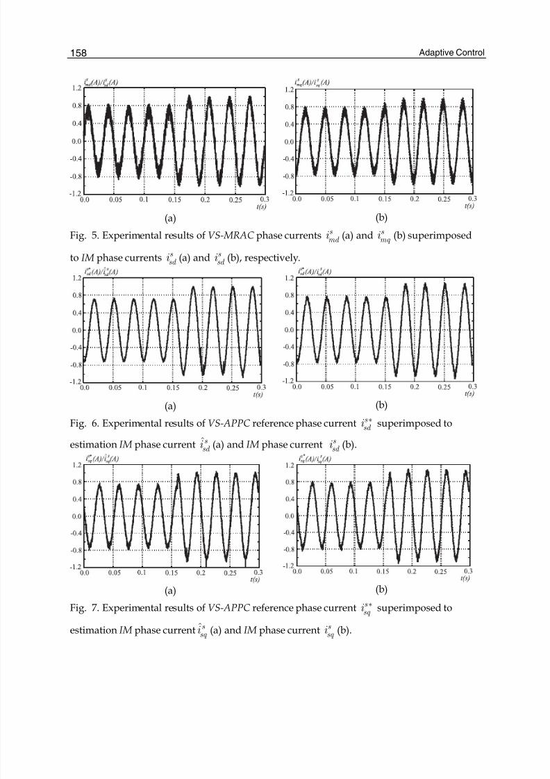
Adaptive Control158
(a) (b)
Fig. 5. Experimental results of VS-MRAC phase currents s md i (a) and s
mq i (b) superimposed
to IM phase currents s sd i (a) and s
sd i (b), respectively.
(a) (b)
Fig. 6. Experimental results of VS-APPC reference phase current s sd i ∗ superimposed to
estimation IM phase current s sd i (a) and IM phase current s
sd i (b).
(a) (b)
Fig. 7. Experimental results of VS-APPC reference phase current s sq i ∗ superimposed to
estimation IM phase current s sq i (a) and IM phase current s
sq i (b).
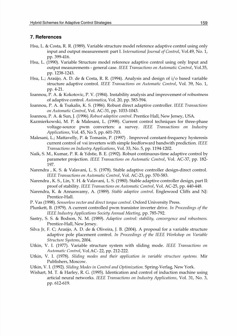
Hybrid Schemes for Adaptive Control Strategies 159
7. References
Hsu, L. & Costa, R. R. (1989). Variable structure model reference adaptive control using onlyinput and output measurement: part I. International Journal of Control, Vol.49, No. 1,pp. 399-416.
Hsu, L. (1990). Variable Structure model reference adaptive control using only Input andoutput measurements - general case. IEEE Transactions on Automatic Control, Vol.35,pp. 1238-1243.
Hsu, L.; Araújo, A. D. de & Costa, R. R. (1994). Analysis and design of i/o based variablestructure adaptive control. IEEE Transactions on Automatic Control, Vol. 39, No. 1,pp. 4-21.
Ioannou, P. A. & Kokotovic, P. V. (1984). Instability analysis and improvement of robustnessof adaptive control. Automatica, Vol. 20, pp. 583-594.
Ioannou, P. A. & Tsakalis, K. S. (1986). Robust direct adaptive controller. IEEE Transactionson Automatic Control, Vol. AC-31, pp. 1033-1043.
Ioannou, P. A. & Sun, J. (1996). Robust adaptive control. Prentice Hall, New Jersey, USA.Kazmierkowski, M. P. & Malesani, L. (1998). Current control techniques for three-phase
voltage-source pwm converters: a survey. IEEE Transactions on Industry Applications, Vol. 45, No 5, pp. 601-703.
Malesani, L.; Mattavelly, P. & Tomasin, P. (1997) . Improved constant-frequency hysteresiscurrent control of vsi inverters with simple feedforward bandwith prediction. IEEETransactions on Industry Applications, Vol. 33, No. 5, pp. 1194-1202.
Naik, S. M., Kumar, P. R. & Ydstie, B. E. (1992). Robust continuous-time adaptive control byparameter projection. IEEE Transactions on Automatic Control, Vol. AC-37, pp. 182-197.
Narendra , K. S. & Valavani, L. S. (1978). Stable adaptive controller design-direct control.IEEE Transactions on Automatic Control, Vol. AC-23, pp. 570-583.
Narendra , K. S., Lin, Y. H. & Valavani, L. S. (1980). Stable adaptive controller design, part II:proof of stability. IEEE Transactions on Automatic Control, Vol. AC-25, pp. 440-448.
Narendra, K. & Annaswamy, A. (1989). Stable adaptive control. Englewood Cliffs and NJ:Prentice-Hall.
P. Vas (1998). Sensorless vector and direct torque control. Oxford University Press.Plunkett, B. (1979). A current controlled pwm transistor inverter drive. In Proceedings of the
IEEE Industry Applications Society Annual Meeting, pp. 785-792.Sastry, S. S. & Bodson, N. M. (1989). Adaptive control: stability, convergence and robustness.
Prentice-Hall, New Jersey.Silva Jr, F. C; Araújo, A. D. de & Oliveira, J. B. (2004). A proposal for a variable structure
adaptive pole placement control. In Proceedings of the IEEE Workshop on VariableStructure Systems, 2004.
Utkin, V. I. (1977). Variable structure system with sliding mode. IEEE Transactions on Automatic Control, Vol.AC- 22, pp. 212-222.
Utkin, V. I. (1978). Sliding modes and their application in variable structure systems. MirPublishers, Moscow.
Utkin, V. I. (1992). Sliding Modes in Control and Optimization. Spring-Verlag, New York.Wishart, M. T. & Harley, R. G. (1995). Identication and control of induction machine using
articial neural networks. IEEE Transactions on Industry Applications, Vol. 31, No. 3,pp. 612-619.

Adaptive Control160
Zhang, C. J. & Dunnigan, M. W. (2003). Robust adaptive stator current control for aninduction machine. In Proceedings of the IEEE Conference Control Applications, pp.779-784.
7
Adaptive Control for Systems with RandomlyMissing Measurements in a Network
Environment
Yang Shi1 and Huazhen Fang1 1Department of Mechanical Engineering, University of Saskatchewan
Canada
1. Introduction
Networked control systems (NCSs) are a type of distributed control systems, where theinformation of control system components (reference input, plant output, control input, etc.)is exchanged via communication networks. Due to the introduction of networks, NCSs havemany attractive advantages, such as reduced system wiring, low weight and space, ease ofsystem diagnosis and maintenance, and increased system agility, which motivated theresearch in NCSs. The study of NCSs has been an active research area in the past severalyears, see some recent survey articles (Chow & Tipsuwan, 2001; Hespanha & Naghshtabrizi,2007; Yang, 2006) and the references therein. On the other hand, the introduction ofnetworks also presents some challenges such as the limited feedback information caused bypacket transmission delays and packet loss; both of them are due to the sharing andcompetition of the transmission medium, and bring difficulties for analysis and design forNCSs. The information transmission delay arises from by the limited capacity of thecommunication network used in a control system, whereas the packet loss is caused by theunavoidable data losses or transmission errors. Both the information transmission delay andpacket loss may result in randomly missing output measurements at the controller node, asshown in Fig. 1. So far different approaches have been used to characterize the limitedfeedback information. For example, the information transmission delay and packet losseshave been modeled as Markov chains (Zhang et al., 2006). The binary Bernoulli distributionis used to model the packet losses in (Sinopoli et al., 2004; Wang et al., 2005 a & 2005 b).The main challenge of NCS design is the limited feedback information (informationtransmission delays and packet losses), which can degrade the performance of systems oreven cause instability. Various methodologies have been proposed for modeling, stabilityanalysis, and controller design for NCSs in the presence of limited feedback information. Anovel feedback stabilization solution of multiple coupled control systems with limitedcommunication is proposed by bringing together communication and control theoreticalissues in (Hristu & Morgansen, 1999). Further the control and communication codesignmethodology is applied in (Hristu-Varsakelis, 2006; Zhang & Hristu-Varsakelis, 2006) – amethod of stabilizing linear NCSs with medium access constraints and transmission delaysby designing a delay-compensated feedback controller and an accompanying medium
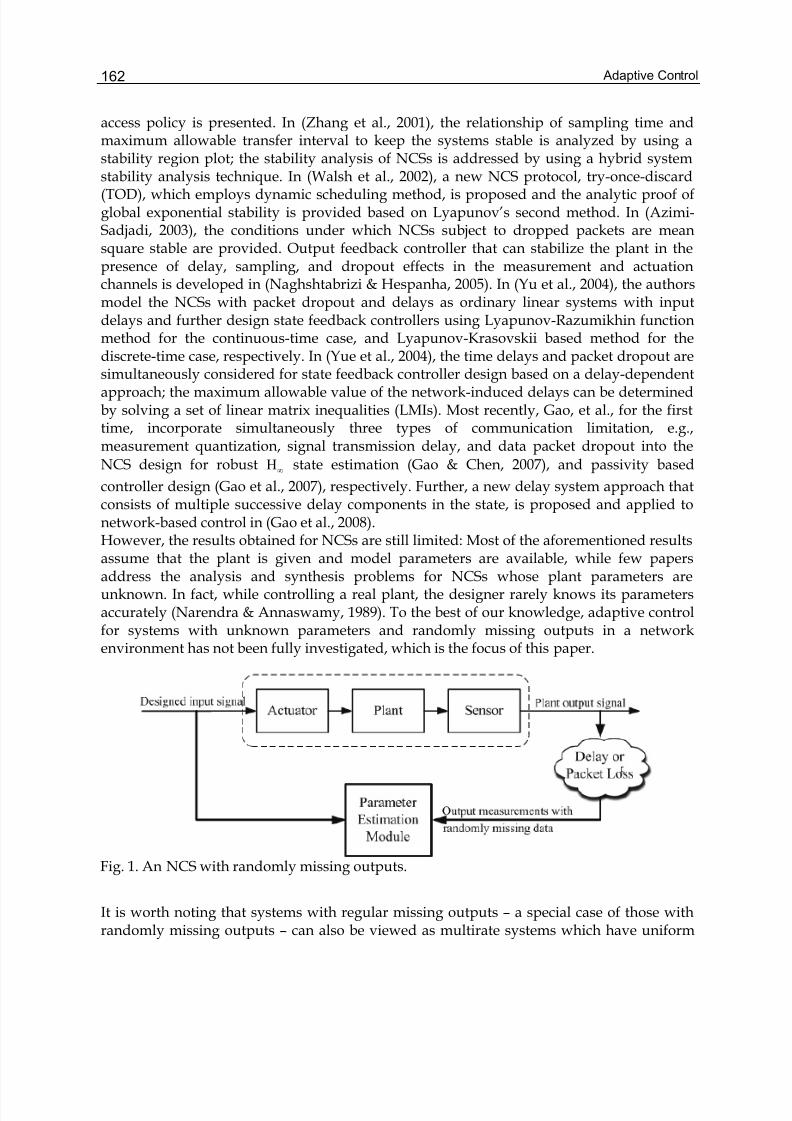
Adaptive Control162
access policy is presented. In (Zhang et al., 2001), the relationship of sampling time andmaximum allowable transfer interval to keep the systems stable is analyzed by using astability region plot; the stability analysis of NCSs is addressed by using a hybrid systemstability analysis technique. In (Walsh et al., 2002), a new NCS protocol, try-once-discard(TOD), which employs dynamic scheduling method, is proposed and the analytic proof ofglobal exponential stability is provided based on Lyapunov’s second method. In (Azimi-Sadjadi, 2003), the conditions under which NCSs subject to dropped packets are meansquare stable are provided. Output feedback controller that can stabilize the plant in thepresence of delay, sampling, and dropout effects in the measurement and actuationchannels is developed in (Naghshtabrizi & Hespanha, 2005). In (Yu et al., 2004), the authorsmodel the NCSs with packet dropout and delays as ordinary linear systems with inputdelays and further design state feedback controllers using Lyapunov-Razumikhin functionmethod for the continuous-time case, and Lyapunov-Krasovskii based method for thediscrete-time case, respectively. In (Yue et al., 2004), the time delays and packet dropout aresimultaneously considered for state feedback controller design based on a delay-dependentapproach; the maximum allowable value of the network-induced delays can be determinedby solving a set of linear matrix inequalities (LMIs). Most recently, Gao, et al., for the firsttime, incorporate simultaneously three types of communication limitation, e.g.,measurement quantization, signal transmission delay, and data packet dropout into the
NCS design for robust ∞H state estimation (Gao & Chen, 2007), and passivity based
controller design (Gao et al., 2007), respectively. Further, a new delay system approach thatconsists of multiple successive delay components in the state, is proposed and applied tonetwork-based control in (Gao et al., 2008).However, the results obtained for NCSs are still limited: Most of the aforementioned resultsassume that the plant is given and model parameters are available, while few papersaddress the analysis and synthesis problems for NCSs whose plant parameters areunknown. In fact, while controlling a real plant, the designer rarely knows its parametersaccurately (Narendra & Annaswamy, 1989). To the best of our knowledge, adaptive controlfor systems with unknown parameters and randomly missing outputs in a networkenvironment has not been fully investigated, which is the focus of this paper.
Fig. 1. An NCS with randomly missing outputs.
It is worth noting that systems with regular missing outputs – a special case of those withrandomly missing outputs – can also be viewed as multirate systems which have uniform
Adaptive Control for Systems with Randomly Missing Measurements in a Network Environment 163
but various input/output sampling rates (Chen & Francis, 1995). Such systems may haveregular-output-missing feature. In (Ding & Chen, 2004a), Ding, et al. use an auxiliary modeland a modified recursive least squares (RLS) algorithm to realize simultaneous parameterand output estimation of dual-rate systems. Further, a least squares based self-tuningcontrol scheme is studied for dual-rate linear systems (Ding & Chen, 2004b) and nonlinearsystems (Ding et al., 2006), respectively. However, network-induced limited feedbackinformation unavoidably results in randomly missing output measurements. To generalizeand extend the adaptive control approach for multirate systems (Ding & Chen, 2004b; Dinget al., 2006) to NCSs with randomly missing output measurements and unknown modelparameters is another motivation of this work.In this paper, we first model the availability of output as a Bernoulli process. Then wedesign an output estimator to online estimate the missing output measurements, and furtherpropose a novel Kalman filter based method for parameter estimation with randomlyoutput missing. Based on the estimated output or the available output, and the estimatedmodel parameters, an adaptive control is proposed to make the output track the desiredsignal. Convergence of the proposed output estimation and adaptive control algorithms isanalyzed.The rest of this paper is organized as follows. The problem of adaptive control for NCSswith unknown model parameters and randomly missing outputs is formulated in Section 2.In Section 3, the proposed algorithms for output estimation, model parameter estimation,and adaptive control are presented. In Section 4, the convergence properties of the proposedalgorithms are analyzed. Section 5 gives several illustrative examples to demonstrate theeffectiveness of the proposed algorithms. Finally, concluding remarks are given in Section 6.
Notations: The notations used throughout the paper are fairly standard.’ E ’ denotes the
expectation. The superscript ‘ T ’ stands for matrix transposition; λ max/min( )X represents the
Maximum/minimum eigenvalue of X ; =| | det( )X X is the determinant of a square matrix
X ; )(2 T
XX tr X = stands forthe trace of TXX . If δ +∃ ∈0 R and +∈0 Zk , δ ≤ 0| ( )| ( ) f k g k
for ≥ 0k k , then ( )=( ) ( ) f k O g k ; if →( ) / ( ) 0 f k g k for → ∞k , then ( )=( ) ( )k o g k .
2. Problem Formulation
The problem of interest in this work is to design an adaptive control scheme for networkedsystems with unknown model parameters and randomly missing outputs. In Fig. 2, the
output measurements ky could be unavailable at the controller node at some time instants
because of the network-induced limited feedback information, e.g., transmission delayand/or packet loss. The data transmission protocols like TCP guarantee the delivery of datapackets in this way: When one or more packets are lost the transmitter retransmits the lostpackets. However, since a retransmitted packet usually has a long delay that is not desirablefor control systems, the retransmitted packets are outdated by the time they arrive at thecontroller (Azimi-Sadjadi, 2003; Hristu-Varsakelis & Levine, 2005). Therefore, in this paper,it is assumed that the output measurements that are delayed in transmission are regarded asmissed ones.
The availability of ky can be viewed as a random variable γ k . γ k is assumed to have Bernoulli
distribution:
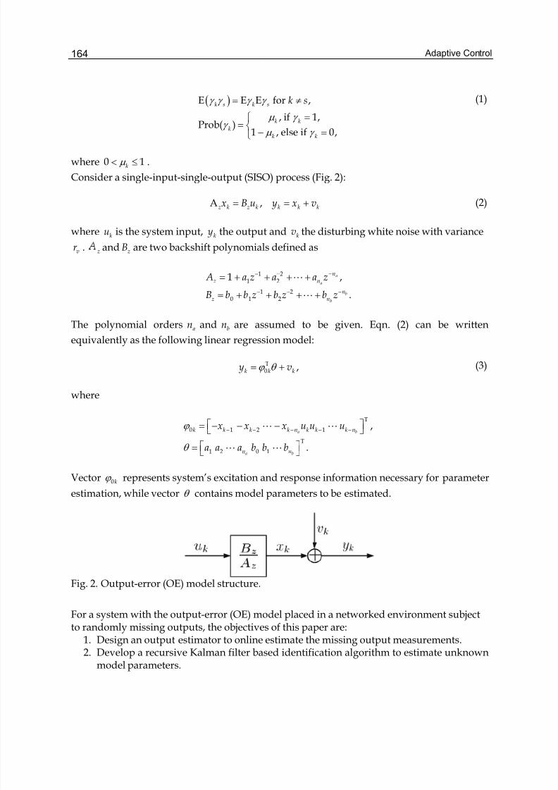
Adaptive Control164
( )γ γ γ γ
μ γ γ
μ γ
= ≠
=⎧⎨⎩
=− =
E E E for ,
, if 1,Prob( )
1 , else if 0,
k s k s
k k
kk k
k s
(1)
where μ < ≤0 1k .
Consider a single-input-single-output (SISO) process (Fig. 2):
= = +A ,z k z k k k kx B u y x v (2)
where ku is the system input, ky the output and kv the disturbing white noise with variance
vr . z and zB are two backshift polynomials defined as
−− −
−− −
= + + + +
= + + + +
L
L
1 21 2
1 20 1 2
,
.
1 a
a
b
b
nz n
nz n
A a z a a z
B b b z b z b z
The polynomial orders an and bn are assumed to be given. Eqn. (2) can be written
equivalently as the following linear regression model:
ϕ θ = +T0 ,k k ky v (3)
where
ϕ
θ
− − − − −⎡ ⎤= − − −⎣ ⎦
⎡ ⎤= ⎣ ⎦
L L
L L
T
0 1 2 1
T
1 2 0 1
,
.
a b
a b
k k k k n k k k n
n n
x x x u u u
a a a b b b
Vector ϕ 0k represents system’s excitation and response information necessary for parameter
estimation, while vector θ contains model parameters to be estimated.
Fig. 2. Output-error (OE) model structure.
For a system with the output-error (OE) model placed in a networked environment subjectto randomly missing outputs, the objectives of this paper are:
1. Design an output estimator to online estimate the missing output measurements.2. Develop a recursive Kalman filter based identification algorithm to estimate unknown
model parameters.
Adaptive Control for Systems with Randomly Missing Measurements in a Network Environment 165
3. Propose an adaptive tracking controller to make the system output track a givendesired signal.
4. Analyze the convergence properties of the proposed algorithms.
3. Parameter Estimation, Output Estimation, and Adaptive Control Design
There are two main challenges of the adaptive control design for a networked system asdepicted in Fig. 1: (1) randomly missing output measurements; (2) unknown system modelparameters. Therefore, in this section, we first propose algorithms for missing outputestimation and unknown model parameter estimation, and then design the adaptive controlscheme.
3.1 Parameter estimation and missing output estimationConsider the model in (3). It is shown by (Cao & Schwartz, 2003) and (Guo, 1990) that thecorresponding Kalman filter can be conveniently used for parameter estimation. Incombination with an auxiliary model, the Kalman filter based parameter estimationalgorithm for an OE model is given by
θ θ ϕ θ − −= + − T1 , , 1
ˆ ˆ ˆ( ),k k a k k a k kK y (4)
ϕ
ϕ ϕ
−
−
=+
, 1 ,, T
, , 1 ,
,a k a ka k
v a k a k a k
PK
r P
(5)
ϕ ϕ
ϕ ϕ
− −−
−
−+
=T
, 1 , , , 1, , 1 T
, , 1 0
,a k a k a k a ka k a k
v a k a k k
P PP P
r P
(6)
φ θ = T, ,
ˆ ,a k a k kx (7)
ϕ − − − − −⎡ ⎤= − − −⎣ ⎦L L
T
, , 1 , 2 , 1 ,a ba k a k a k a k n k k k nx x x u u u (8)
where θ k represents the estimated parameter vector at time instant k .
It is worth to note that the above algorithm as shown in (4)-(8) cannot be directly applied tothe parameter estimation of systems with randomly missing outputs in a network
environment, as ky in (4) may not be available. This motivates us to develop a new
algorithm that can simultaneously online estimate the unavailable missing output andestimate system parameters under the network environment. The proposed algorithmconsists of two steps.
Step 1: Output estimationAlbertos, et al. propose a simple algorithm that uses the input-output model, replacing theunknown past values by estimates when necessary (Albertos et al., 2006). Inspired by thiswork, we design the following output estimator:
Adaptive Control166
γ γ = + − ˆ(1 ) ,k k k k kz y y (9)
with
ϕ θ −= T1
ˆˆ .k k ky
In (9), γ k is a Bernoulli random variable used to characterize the availability of ky at time
instant k at the controller node, as defined in (1). With the time-stamp technique, the
controller node can detect the availability of the output measurements, and thus, the values
of γ k (either 1 or 0) are known. The knowledge of their corresponding probability μ k is not
used in the designed estimator. The structure of the designed output estimator is intuitiveand simple yet very effective, which will be seen soon from the simulation examples.
Step 2: Model parameter estimation
Replacing ky in the algorithm (4)-(8) by kz , defining a newϕ k , and considering the random
variableγ k , we readily obtain the following algorithm:
θ θ ϕ θ − −= + − T1 1
ˆ ˆ ˆ( ),k k k k k kK z (10)
ϕ
ϕ ϕ
−
−
=+
1T
1
,k kk
v k k k
PK
r P
(11)
ϕ ϕ γ
ϕ ϕ
− −−
−
= −+
T1 1
1 T1
,k k k kk k k
v k k k
P PP P
r P
(12)
ϕ θ = T,
ˆ ,b k k kx (13)
ϕ − − − − −⎡ ⎤= − − −⎣ ⎦L L
T
, 1 , 2 , 1 .a bk b k b k b k n k k k nx x x u u u (14)
Remark 3.1. Consider two extreme cases. If the availability sequence γ γ L1 , , k constantly assumes
1, then no output measurement is lost, and the algorithm above will reduce to the algorithm (4)-(6).
On the other hand, if the availability sequence γ k constantly takes 0, then all output measurements
are lost, and the parameter estimates just keep the initial values.
3.2 Adaptive control design Consider the tracking problem. Let ,r ky be a desired output signal, and define the output
tracking error
ζ = − ,: .k k r ky y
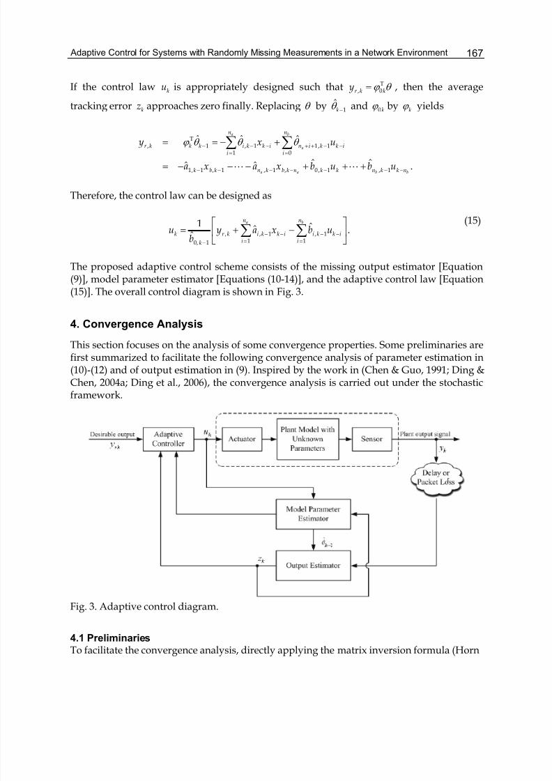
Adaptive Control for Systems with Randomly Missing Measurements in a Network Environment 167
If the control law ku is appropriately designed such that ϕ θ = T, 0r k ky , then the average
tracking error kz approaches zero finally. Replacing θ by θ −1ˆk and ϕ 0k by ϕ k yields
ϕ θ θ θ − − − + + − −= =
− − − − − − −
= = − +
= − − − + + +
∑ ∑
L L
T, 1 , 1 1, 1
1 0
1, 1 , 1 , 1 , 0 , 1 , 1
ˆ ˆ ˆ
ˆ ˆˆ ˆ .
a b
a
a a b b
n n
r k k k i k k i n i k k ii i
k b k n k b k n k k n k k n
y x u
a a b u b ux x
Therefore, the control law can be designed as
− − − −= =−
⎡ ⎤= + −⎢ ⎥
⎣ ⎦∑ ∑, , 1 , 1
1 10, 1
1 ˆˆ .ˆ
a bn n
k r k i k k i i k k ii ik
u y a x b ub
(15)
The proposed adaptive control scheme consists of the missing output estimator [Equation(9)], model parameter estimator [Equations (10-14)], and the adaptive control law [Equation(15)]. The overall control diagram is shown in Fig. 3.
4. Convergence Analysis
This section focuses on the analysis of some convergence properties. Some preliminaries arefirst summarized to facilitate the following convergence analysis of parameter estimation in(10)-(12) and of output estimation in (9). Inspired by the work in (Chen & Guo, 1991; Ding &Chen, 2004a; Ding et al., 2006), the convergence analysis is carried out under the stochasticframework.
Fig. 3. Adaptive control diagram.
4.1 Preliminaries
To facilitate the convergence analysis, directly applying the matrix inversion formula (Horn
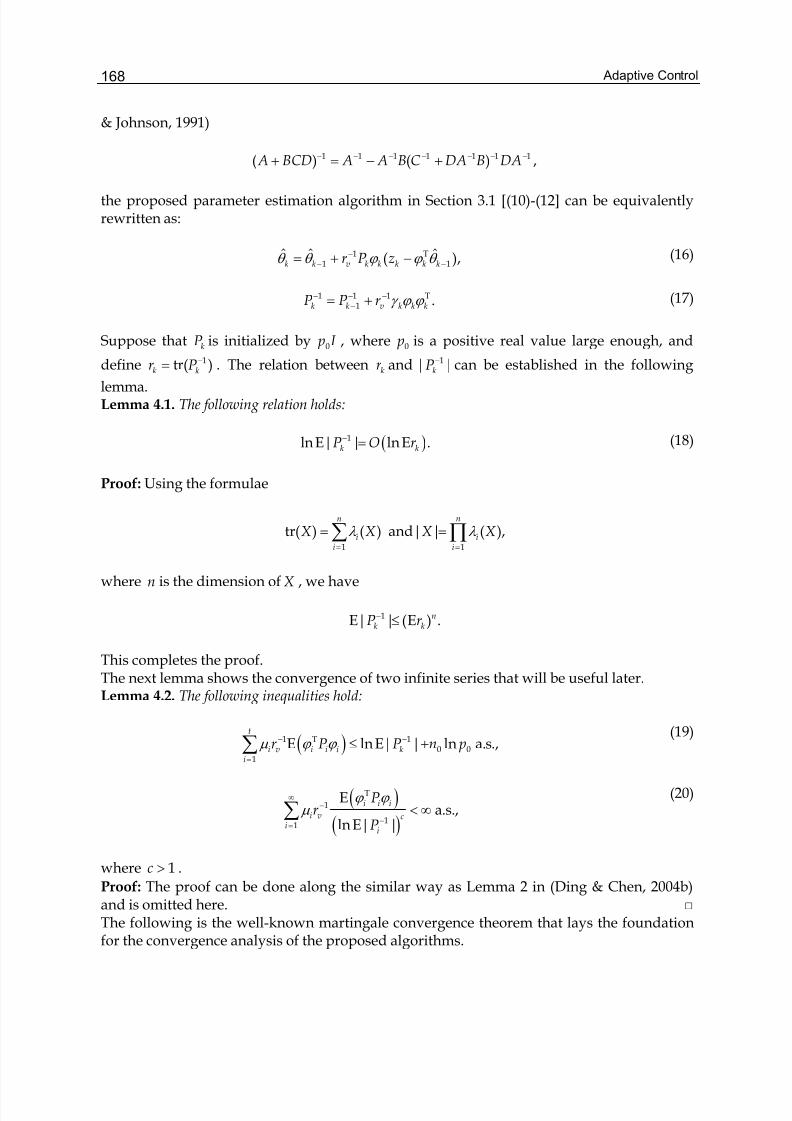
Adaptive Control168
& Johnson, 1991)
− − − − − − −+ = − +1 1 1 1 1 1 1( ) ( ) , A BCD A A B C DA B DA
the proposed parameter estimation algorithm in Section 3.1 [(10)-(12] can be equivalentlyrewritten as:
θ θ ϕ ϕ θ −− −= + −1 T
1 1ˆ ˆ ˆ( ),k k v k k k k kr P z (16)
γ ϕ ϕ − − −−= +1 1 1 T
1 .k k v k k kP P r (17)
Suppose that kP is initialized by 0 p I , where 0 p is a positive real value large enough, and
define −= 1tr( )k kr P . The relation between kr and −1| |kP can be established in the following
lemma.Lemma 4.1. The following relation holds:
( )− =1ln E| | ln E .k kP O r (18)
Proof: Using the formulae
λ λ = =
= =∑ ∏1 1
tr( ) ( ) and| | ( ),nn
i ii i
X X X X
where n is the dimension of X , we have
− ≤1E| | (E ) .nk kP r
This completes the proof.The next lemma shows the convergence of two infinite series that will be useful later.Lemma 4.2. The following inequalities hold:
( )μ ϕ ϕ − −
=
≤ +∑ 1 T 10 0
1
E ln E| | ln a.s.,t
i v i i i ki
r P P n p (19)
( )
( )
ϕ ϕ μ
∞−
−=
< ∞∑T
1
11
Ea.s.,
ln E| |
i i i
i v ci
i
Pr
P
(20)
where > 1c .
Proof: The proof can be done along the similar way as Lemma 2 in (Ding & Chen, 2004b)and is omitted here. The following is the well-known martingale convergence theorem that lays the foundationfor the convergence analysis of the proposed algorithms.
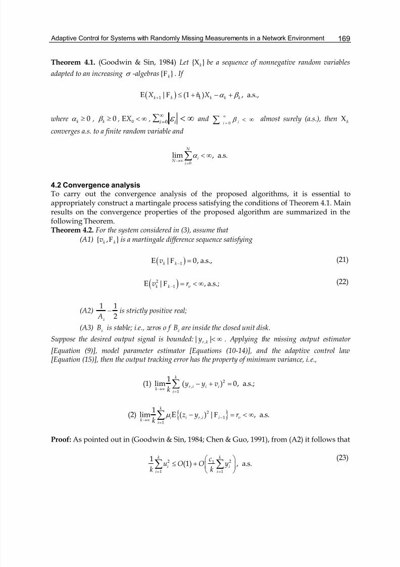
Adaptive Control for Systems with Randomly Missing Measurements in a Network Environment 169
Theorem 4.1. (Goodwin & Sin, 1984) Let X k be a sequence of nonnegative random variables
adapted to an increasing σ -algebras kF . If
( ) α β + ≤ + − +1E | (1 ) , a.s.,k k k k k kX X F ň
where α ≥ 0k , β ≥ 0k , < ∞0EX , ∞<∑∞= iiε 0 and β
∞
=< ∞∑ 0 ii
almost surely (a.s.), then Xk
converges a.s. to a finite random variable and
α →∞
=
< ∞∑0
lim , a.s.N
iN
i
4.2 Convergence analysisTo carry out the convergence analysis of the proposed algorithms, it is essential toappropriately construct a martingale process satisfying the conditions of Theorem 4.1. Mainresults on the convergence properties of the proposed algorithm are summarized in thefollowing Theorem.Theorem 4.2. For the system considered in (3), assume that
(A1) , k kv F is a martingale difference sequence satisfying
( )− =1E | 0, a.s.,k kv F (21)
( )− = < ∞21E | , a.s.;k k vv r F (22)
(A2) −1 1
2z Ais strictly positive real;
(A3) zB is stable; i.e., zeros o f zB are inside the closed unit disk.
Suppose the desired output signal is bounded: < ∞,| |r ky . Applying the missing output estimator
[Equation (9)], model parameter estimator [Equations (10-14)], and the adaptive control law[Equation (15)], then the output tracking error has the property of minimum variance, i.e.,
(1)→∞
=
− + =∑ 2,
1
1lim ( ) 0, a.s.;
k
r i i ik
i
y y vk
(2) μ −→∞
=
− = < ∞∑ 2, 1
1
1lim E ( ) | , a.s.
k
i i r i i vk
i
z y r k
F
Proof: As pointed out in (Goodwin & Sin, 1984; Chen & Guo, 1991), from (A2) it follows that
= =
⎛ ⎞≤ + ⎜ ⎟
⎝ ⎠∑ ∑2 21
1 1
1(1) , a.s.
k k
i ii i
cu O O y
k k
(23)
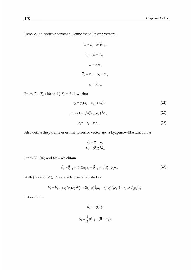
Adaptive Control170
Here, 1c is a positive constant. Define the following vectors:
ϕ θ −= − T1 ,ˆ
k k ke z
η = − , ,k k b ky x
η γ η = ,k k k
τ = − +, ,k r k k ky y v
τ γ τ = .k k k
From (2), (3), (16) and (16), it follows that
η γ = − +,( ),k k k b k kx x v (24)
η ϕ ϕ − −−= + 1 T 1
1(1 ) ,k v k k k kr P e (25)
τ γ − += .k k k ke v (26)
Also define the parameter estimation error vector and a Lyapunov-like function as
θ θ θ = −% ˆ ,k k
θ θ −= % %T 1 .k k k kV P
From (9), (16) and (25), we obtain
θ θ ϕ θ ϕ η − −− − −+ +=% % %1 1
1 1 1= .k k v k k k k v k k kr P e r P (27)
With (17) and (27), kV can be further evaluated as
γ ϕ θ ϕ θ η ϕ ϕ ϕ ϕ − − − −−= + + − −% %1 T 2 1 T 2 T 1 T 2
1 ( ) 2 (1 ) .k k v k k k v k k k v k k k v k k k kV V r r r P r P e
Let us define
ϕ θ −= %%T ,k k ku
ϕ θ η −= +%%T1
( ).2
k k k k ky v
Adaptive Control for Systems with Randomly Missing Measurements in a Network Environment 171
Then we have
γ γ ϕ θ ϕ ϕ ϕ ϕ
γ γ ϕ θ ϕ ϕ γ γ
ϕ ϕ ϕ ϕ τ ϕ ϕ ϕ ϕ τ
− − − −−
− − −− −
− − − −
= − + − −
⎡ ⎤= − + + − +⎣ ⎦
− − + −
%% %
%% %
1 1 T 2 T 1 T 21
1 1 T 2 T T 21 1
2 T 1 T 2 2 T 1 T
2 2 (1 )
2 2 2 ( )
(1 ) 2 (1 )
k k v k k k v k k k k v k k k v k k k k
k v k k k v k k k k v k k k k k k k k k
v k k k v k k k k v k k k v k k k k
V V r u y r v r P r P e
V r u y r v r P e v v v
r P r P r P r P v
ϕ ϕ ϕ ϕ
γ γ ϕ θ ϕ ϕ γ γ
ϕ ϕ ϕ ϕ τ ϕ ϕ ϕ ϕ τ
− −
− − −− −
− − − −
− −
⎡ ⎤≤ − + + − +⎣ ⎦
− − + −
%% %
2 T 1 T 2
1 1 T 2 T T 21 1
2 T 1 T 2 2 T 1 T
(1 )
2 2 2 ( )
(1 ) 2 (1 ) .
k
v k k k v k k k k
k v k k k v k k k k v k k k k k k k k k
v k k k v k k k k v k k k v k k k k k
r P r P v
V r u y r v r P e v v v
r P r P r P r P v
(28)
Note that ϕ θ −%T
1k k , γ −k k ke v ,ϕ ϕ Tk k kP andτ k are uncorrelated with kv and −1kF -measurable. Thus
taking the conditional expectation of both sides of (28) with respect to −1kF gives
( ) ( ) ( )μ μ ϕ ϕ
μ ϕ ϕ ϕ ϕ τ
− −− −
− −
≤ − +
⎡ ⎤− −⎣ ⎦
% %1 1 T
1 1
2 T 1 T 2
E | 2 E 2 E
E (1 ) .
k k k v k k k v k k k k
v k k k k v k k k k
V V r u y r P
r P r P
F
(29)
Consider that
η
ϕ θ
− = −
= −
= − =% %
,
,
T
( ) ( )
.
z k k z k b k
z k z b k
k k k
A v A y x
B u A x
u
Therefore, we have
⎛ ⎞= −⎜ ⎟⎝ ⎠
% %1 1
.2
k k
z
y u A
In (A2), it is assumed that⎛ ⎞
−⎜ ⎟⎝ ⎠
1 1
2z Ais positive real, which indicates
μ −
=
≥= ∑ % %1
1
2 0, a.s.:k
k v k k ki
S r u y (30)
Adding kS to both sides of (29) yields
( ) ( )μ ϕ ϕ
μ ϕ ϕ ϕ ϕ τ
−− − −
− −
+ ≤ + +
⎡ ⎤− −⎣ ⎦
1 T1 1 1
2 T 1 T 2
E | 2 E
E (1 ) .
k k k k k v k k k k
v k k k k v k k k k
V S V S r P
r P r P
F
(31)
Define a new sequence:
Adaptive Control172
( )−
+= >
1, 1.
ln E| |
k kk c
k
V SW c
P
(32)
Since −1ln E| |kP is nondecreasing andϕ ϕ =T (1)k k kP o , there exists a 0k such that if ≥ 0k k we
have
( )( )
( )
( )
( )
( )
( )
( )
( )
μ ϕ ϕ
μ ϕ ϕ ϕ ϕ τ
μ ϕ ϕ
μ ϕ ϕ τ
−
− −−
− −
− −
−
−
−−
− −
−
+≤ +
⎡ ⎤−⎣ ⎦−
≤ +
−−
1 T
1 11
1 1
2 T 1 T 2
1
1 T
11
2 1 T 2
1
2 EE |
ln E| | ln E| |
E (1 )
ln E| |
2 E
ln E| |
E 1.
ln E| |
v k k k kk kk k c c
k k
v k k k k v k k k k
c
k
v k k k k
k c
k
v k v k k k k
c
k
r PV SW
P P
r P r P
P
r PW
P
r r P
P
F
(33)
From (12) we have
( )ϕ ϕ −− >1 TE 1 0.v k k kr P
Also note that by Lemma 4.2 the summation of the third term in (33) from 0 to ∞ is finite.Therefore, Theorem 4.1 is applicable, and it gives
( )
( )
μ ϕ ϕ τ − −∞
−=
−< ∞∑
2 1 T 2
11
E 1a.s.
ln | |
v k v k k k k
ck
k
r r P
E P (34)
Further, Lemma 4.1 indicates
( )( )
μ ϕ ϕ τ − −∞
=
−< ∞∑
2 1 T 2
1
E 1a.s.
ln E
v k v k k k k
ck k
r r P
r (35)
As ( )ϕ ϕ −⎡ ⎤−⎣ ⎦1 T1 Ev k k kr P is positive and nondecreasing, it holds that ( )ϕ ϕ −⎡ ⎤= −⎣ ⎦
1 T1 1 Ev k k kO r P .
Hence,
( )
τ ∞
=
< ∞∑2
1
a.s.ln E
ic
i ir (36)
Since →∞ = ∞lim ln Ek kr , then from the Kronecker lemma [15] it follows that
Adaptive Control for Systems with Randomly Missing Measurements in a Network Environment 173
→∞Δ =lim 0, a.s.,k
k
where
τ =
Δ = ∑ 2
1
1.
(ln E ):
k
k icikr
With
γ ϕ ϕ
−
=
= +∑1
T
10
k
k i i ii v
nr r
p
and (23), we obtain
[ ]
τ
μ
=
= =
=
Δ⎡ ⎤= ⎣ ⎦
Δ=
⎛ ⎞Δ= + +⎜ ⎟
⎝ ⎠
⎛ ⎞= Δ ⎜ ⎟
⎝ ⎠
∑
∑ ∑
∑
2
1
2 2
1 10
2
1
1(ln E )
E( )
E ( )
1
kck
i ki
kk
k kk
a i i b ii i
k
k ii
O r k k
O r k
nO n z n u
k p
O yk
(37)
By (22) we have
η = =
⎛ ⎞= + ⎜ ⎟
⎝ ⎠∑ ∑2 2
1 1
1 1(1) .
k k
i ii i
y O Ok k
(38)
Substituting (37) into (38) gives
=
=∑ 2
1
1(1), a.s.,
k
ii
y Ok
which implies together with (37) that
τ →∞
=
=∑ 2
1
1lim 0, a.s.,
k
ik
ik
or equivalently
Adaptive Control174
→∞=
=− +∑ 2,
1
1lim ( ) 0, a.s.
k
r i i ik
i
y y vk
(39)
Since
− −
−
−
− + = − + − +
= − + − +
= − −
2 2 2, 1 , , 1
2, 1
2, 1
E ( ) | E[( ) 2 2 | ]
E[( ) |
] 0 2
E[( ) | ] , a.s.,
r k k k k r k k r k k k k k k
r k k k v v
r k k k v
y y v y y y v y v v
y y r r
y y r
F F
F
F
and γ γ =k k k kz y , we have
μ μ − −→∞ →∞
= =
− = − =∑ ∑2 2, 1 , 1
1 1
1 1lim E ( ) | lim E ( ) | , a.s.
k k
i i r i i i i r i i vk k
i i
z y y y r k k
F F
This completes the proof.
5. Illustrative Examples
In this section, we give three examples to illustrate the adaptive control design schemeproposed in the previous sections.The OE model shown in Fig. 2 in the simulation is chosen as
− −
− −
+ += +
+ +
1 20 1 2
1 21 2
,1
k k k
b b z b zy u v
a z a z
which is assumed to be placed in a network environment (Fig. 1) with randomly missing
output measurements and unknown model parameters. kv is a Gaussian white noise
sequence with zero mean and variance = 20.05vr . The parameter vector θ = T1 2 0 1 2[ ]a a b b b is
to be estimated. Here, true values of θ are
θ = − T[ 0.3 0.6 0.5 0.2 0.34] .
For simulation purposes, we assume that: (1) θ is unknown and initialized by ones; (2) the
output measurement ky is subject to randomly missing when transmitted to the controller
node; (3) the availability of the output measurements ( ky ) at the controller node is
characterized by the probability μ k ; (4) The desired output signal to be tracked is a square
wave alternating between -1 and 1 with a period of 1000. Mathematically, it is given by
++ = − = =L
1,(500 ) ( 1) , 0,1,2, , 1,2,...500.i
r i jy i j
In the following simulation studies, we carry out experiments for three different scenarios
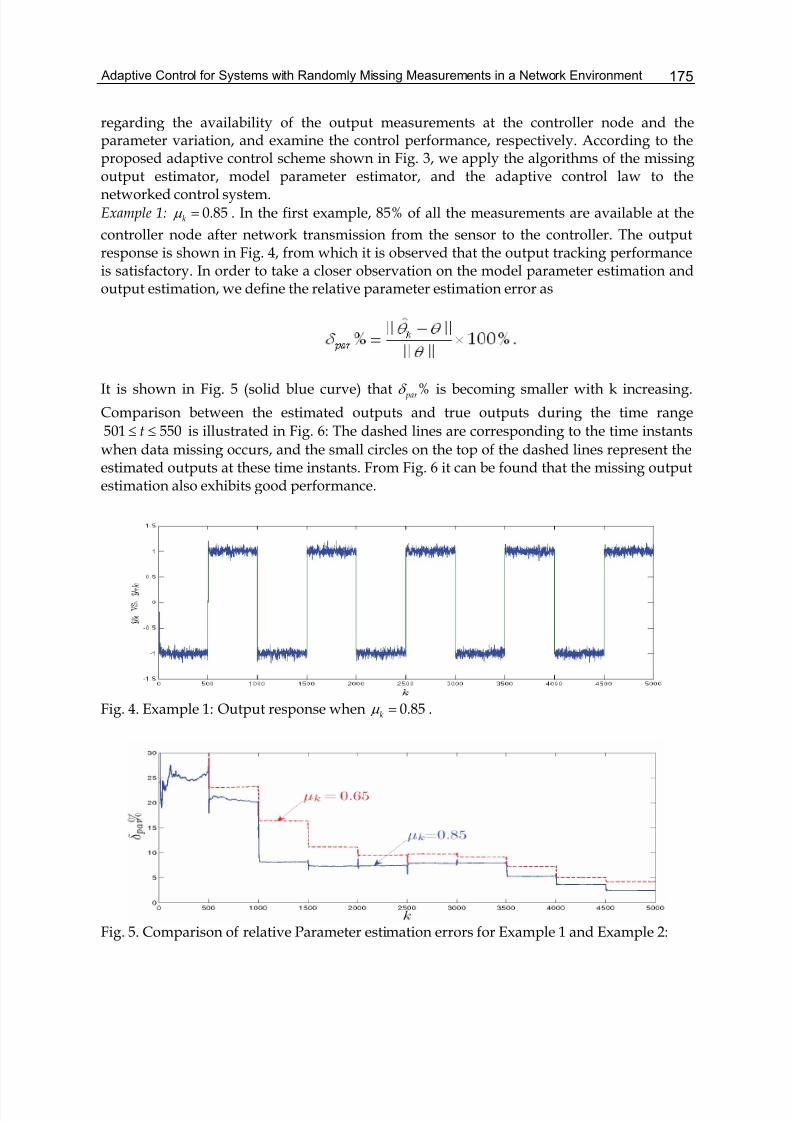
Adaptive Control for Systems with Randomly Missing Measurements in a Network Environment 175
regarding the availability of the output measurements at the controller node and theparameter variation, and examine the control performance, respectively. According to theproposed adaptive control scheme shown in Fig. 3, we apply the algorithms of the missingoutput estimator, model parameter estimator, and the adaptive control law to thenetworked control system.
Example 1: μ = 0.85k . In the first example, 85% of all the measurements are available at the
controller node after network transmission from the sensor to the controller. The outputresponse is shown in Fig. 4, from which it is observed that the output tracking performanceis satisfactory. In order to take a closer observation on the model parameter estimation andoutput estimation, we define the relative parameter estimation error as
It is shown in Fig. 5 (solid blue curve) that δ % par is becoming smaller with k increasing.
Comparison between the estimated outputs and true outputs during the time range
≤ ≤501 550t is illustrated in Fig. 6: The dashed lines are corresponding to the time instants
when data missing occurs, and the small circles on the top of the dashed lines represent theestimated outputs at these time instants. From Fig. 6 it can be found that the missing outputestimation also exhibits good performance.
Fig. 4. Example 1: Output response when μ = 0.85k .
Fig. 5. Comparison of relative Parameter estimation errors for Example 1 and Example 2:
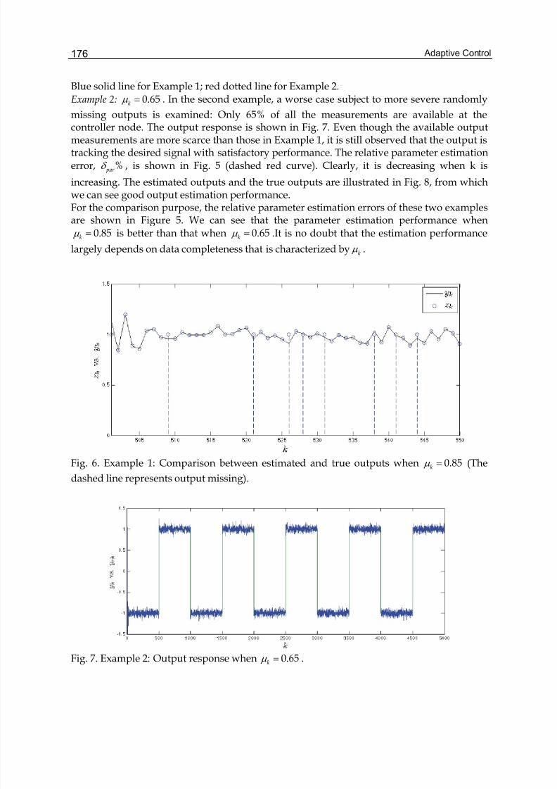
Adaptive Control176
Blue solid line for Example 1; red dotted line for Example 2.
Example 2: μ = 0.65k . In the second example, a worse case subject to more severe randomly
missing outputs is examined: Only 65% of all the measurements are available at thecontroller node. The output response is shown in Fig. 7. Even though the available outputmeasurements are more scarce than those in Example 1, it is still observed that the output istracking the desired signal with satisfactory performance. The relative parameter estimationerror, δ % par , is shown in Fig. 5 (dashed red curve). Clearly, it is decreasing when k is
increasing. The estimated outputs and the true outputs are illustrated in Fig. 8, from whichwe can see good output estimation performance.For the comparison purpose, the relative parameter estimation errors of these two examplesare shown in Figure 5. We can see that the parameter estimation performance when
μ = 0.85k is better than that when μ = 0.65k .It is no doubt that the estimation performance
largely depends on data completeness that is characterized byμ k .
Fig. 6. Example 1: Comparison between estimated and true outputs when μ = 0.85k (The
dashed line represents output missing).
Fig. 7. Example 2: Output response when μ = 0.65k .
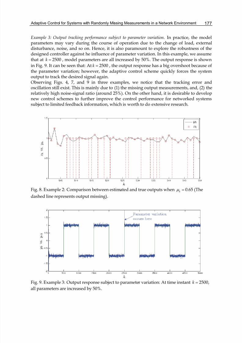
Adaptive Control for Systems with Randomly Missing Measurements in a Network Environment 177
Example 3: Output tracking performance subject to parameter variation. In practice, the modelparameters may vary during the course of operation due to the change of load, externaldisturbance, noise, and so on. Hence, it is also paramount to explore the robustness of thedesigned controller against he influence of parameter variation. In this example, we assume
that at = 2500k , model parameters are all increased by 50%. The output response is shown
in Fig. 9. It can be seen that: At = 2500k , the output response has a big overshoot because of
the parameter variation; however, the adaptive control scheme quickly forces the systemoutput to track the desired signal again.Observing Figs. 4, 7, and 9 in three examples, we notice that the tracking error andoscillation still exist. This is mainly due to (1) the missing output measurements, and, (2) therelatively high noise-signal ratio (around 25%). On the other hand, it is desirable to developnew control schemes to further improve the control performance for networked systemssubject to limited feedback information, which is worth to do extensive research.
Fig. 8. Example 2: Comparison between estimated and true outputs when μ = 0.65k (The
dashed line represents output missing).
Fig. 9. Example 3: Output response subject to parameter variation: At time instant = 2500,k
all parameters are increased by 50%.
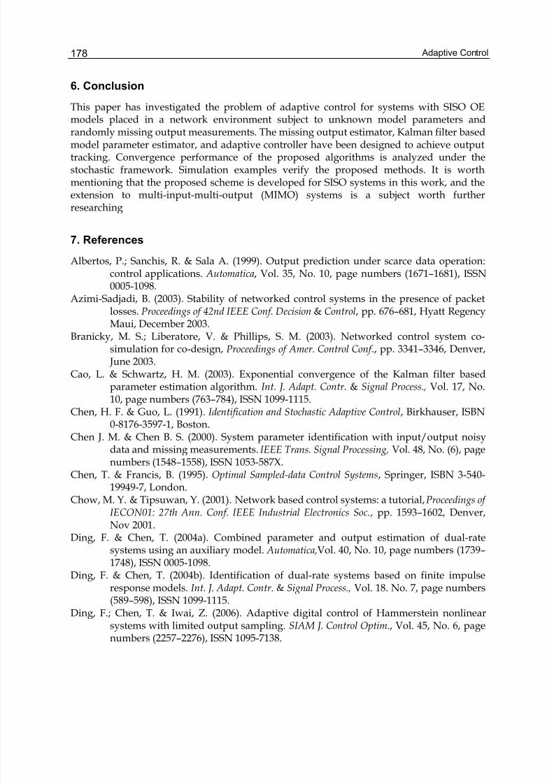
Adaptive Control178
6. Conclusion
This paper has investigated the problem of adaptive control for systems with SISO OEmodels placed in a network environment subject to unknown model parameters andrandomly missing output measurements. The missing output estimator, Kalman filter basedmodel parameter estimator, and adaptive controller have been designed to achieve outputtracking. Convergence performance of the proposed algorithms is analyzed under thestochastic framework. Simulation examples verify the proposed methods. It is worthmentioning that the proposed scheme is developed for SISO systems in this work, and theextension to multi-input-multi-output (MIMO) systems is a subject worth furtherresearching
7. References
Albertos, P.; Sanchis, R. & Sala A. (1999). Output prediction under scarce data operation:control applications. Automatica, Vol. 35, No. 10, page numbers (1671–1681), ISSN0005-1098.
Azimi-Sadjadi, B. (2003). Stability of networked control systems in the presence of packetlosses. Proceedings of 42nd IEEE Conf. Decision & Control, pp. 676–681, Hyatt RegencyMaui, December 2003.
Branicky, M. S.; Liberatore, V. & Phillips, S. M. (2003). Networked control system co-simulation for co-design, Proceedings of Amer. Control Conf ., pp. 3341–3346, Denver, June 2003.
Cao, L. & Schwartz, H. M. (2003). Exponential convergence of the Kalman filter basedparameter estimation algorithm. Int. J. Adapt. Contr. & Signal Process., Vol. 17, No.10, page numbers (763–784), ISSN 1099-1115.
Chen, H. F. & Guo, L. (1991). Identification and Stochastic Adaptive Control, Birkhauser, ISBN0-8176-3597-1, Boston.
Chen J. M. & Chen B. S. (2000). System parameter identification with input/output noisydata and missing measurements. IEEE Trans. Signal Processing, Vol. 48, No. (6), pagenumbers (1548–1558), ISSN 1053-587X.
Chen, T. & Francis, B. (1995). Optimal Sampled-data Control Systems, Springer, ISBN 3-540-19949-7, London.
Chow, M. Y. & Tipsuwan, Y. (2001). Network based control systems: a tutorial,Proceedings of IECON01: 27th Ann. Conf. IEEE Industrial Electronics Soc., pp. 1593–1602, Denver,Nov 2001.
Ding, F. & Chen, T. (2004a). Combined parameter and output estimation of dual-ratesystems using an auxiliary model. Automatica,Vol. 40, No. 10, page numbers (1739–1748), ISSN 0005-1098.
Ding, F. & Chen, T. (2004b). Identification of dual-rate systems based on finite impulseresponse models. Int. J. Adapt. Contr. & Signal Process., Vol. 18. No. 7, page numbers(589–598), ISSN 1099-1115.
Ding, F.; Chen, T. & Iwai, Z. (2006). Adaptive digital control of Hammerstein nonlinearsystems with limited output sampling. SIAM J. Control Optim., Vol. 45, No. 6, pagenumbers (2257–2276), ISSN 1095-7138.
Adaptive Control for Systems with Randomly Missing Measurements in a Network Environment 179
Gao, H. & Chen, T. (2007). H ∞ estimation for uncertain systems with limited communication
capcaity. IEEE Trans. Automat. Contr., Vol. 52, No. 11, page numbers (2070–2084),ISSN 0018-9286.
Gao, H.; Chen, T. & Chai, TY. (2007). Passivity and passification for networked controlsystems. SIAM J. Control Optim., Vol. 46, No. 4, page numbers (1299–1322), ISSN1095-7138.
Gao, H.; Chen, T. & Lam, J. (2008). A new delay system approach to network-based control. Automatica, Vol. 44, No. 1, page numbers (39–52), ISSN 0005-1098.
Goodwin, G. C. & Sin, K. S. (1984) Adaptive Filtering, Prediction and Control, Prentice Hall,ISBN-13: 978-0130040695, Englewood Cliffs.
Guo, L. (1990). Estimating time-varying parameters by the Kalman filter based algorithm:stability and convergence. IEEE Trans. Automat. Contr., Vol. 35, No. 2, pagenumbers (141–147), ISSN 0018-9286.
Hespanha, J. P.; Naghshtabrizi, P. & Xu, P. (2007). A survery of recent results in networkedcontrol systems. Proc. of the IEEE, Vol. 95, No. 1, page numbers (138–162), ISSN0018- 9219.
Horn, R. A. & Johnson, C. R. (1991). Topics in Matrix Analysis, Cambridge University Press,ISBN-13: 9780521467131, Cambridge.
Hristu, D. & Morgansen, K. (1999). Limited communication control. Systems & ControlLetters, Vol. 37, No. 4, page numbers (193–205), ISSN 0167-6911.
Hristu-Varsakelis, D. & Levine, W. S. (2005). Handbook of Networked and Embedded ControlSystems, Birkhauser, ISBN: 978-0-8176-3239-7.
Hristu-Varsakelis, D. (2006). Stabilization of networked control systems with accessconstraints and delays. Proceedings of 45th IEEE Conf. Decision & Control, pp. 1123–1128, San Diego, December 2006.
Isaksson, A. J. (1993). Identification of ARX-models subject to missing data. IEEE Trans. Automat. Contr, Vol. 38, No. 5, page numbers (813–819), ISSN 0018-9286.
Kao, C. Y. & Lincoln, B. (2004). Simple stability criteria for systems with time-varyingdelays, Automatica, Vol. 40, No. 8, page numbers (1429–1434), ISSN 0005-1098.
Lian, F. L.; Moyne, J. & Tilbury, D. (2002). Network design consideration for distributedcontrol systems. IEEE Trans. Contr. Syst. Technol, Vol. 10, No. 2, page numbers (297–307), ISSN 1558-0865.
Naghshtabrizi, P. & Hespanha, J. P. (2005). Designing an observer-based controller for anetwork control system. Proceedings of 44th IEEE Conf. Decision & Control, andEuropean Control Conf., pp. 848–853, Seville December 2005.
Narendra, K. S. & Annaswamy, A. M. (1989). Stable Adaptive Systems, Dover Publications,ISBN 9780486442266.
Nilsson, J. (1998). Real-time Control Systems with Delays, Ph.D. Thesis, Lund Institute ofTechnology.
Shi, Y.; Fang, H. & Yan, M. (2008). Kalman filter-based adaptive control for networkedsystems with unknown parameters and randomly missing outputs. Int. J. RobustNonlinear Contol. In press, DOI: 10.1002/rnc.1390.
Sinopoli, B.; Schenato, L.; Franceschetti, M.; Poolla, K.; Jordan, M. I. & Sastry, S. S. (2004).Kalman filtering with intermittent observations. IEEE Trans. Autom. Contr . Vol. 49,No. 9, page numbers (1453–1464), ISSN 1558-0865.
Adaptive Control180
Wallin, R.; Isaksson, A. J. & Noreus, O. (2001). Extension to “Output prediction under scarcedata operation: control applications”. Automatica, Vol. 37, No. 12, page numbers(2069–2071), ISSN 0005-1098.
Walsh, G. C. & Ye, H. (2001). Scheduling of networked control systems. IEEE Control Syst. Mag. Vol. 21, No. 1, page numbers (57-65), ISSN 0272-1708.
Walsh, G. C.; Ye, H. & Bushnell, L. G. (2002). Stability analysis of networked controlsystems. IEEE Trans. Contr. Syst. Technol., Vol. 10, No. 3, page numbers (438–446),ISSN 1558-0865.
Wang, Z. D.; Yang, F.; Ho, D. W. C. & Liu, X. (2005a). Robust finite-horizon filtering forstochastic systems with missing measurements. IEEE Signal Process. Lett., Vol. 12,No. 6, page numbers (437–440), ISSN: 1558-2361.
Wang, Z. D.; Yang, F.; Ho, D. W. C. & Liu, X. (2005b). Variance-constrained control foruncertain stochastic systems with missing measurement. IEEE Trans. Syst. ManCybern. A, Syst. Humans, Vol. 35, No. 5, page numbers (746–753), ISSN: 1083-4427.
Wu, J. & Chen, T. (2007). Design of networked control systems with packet dropouts. IEEETrans. Automat. Contr., Vol. 52, No. 7, page numbers (1314–1319), ISSN 1558-0865.
Yang, T. C. (2006). Networked control system: a brief survey. IEE Proc. Contr. Theory Appl.,Vol. 153, No. 4, page numbers (403–412), ISSN 1350-2379.
Yu, M.; Wang, L.; Chu, T. & Hao, F. (2004). An LMI approach to networked control systemswith data packet dropout and transmission delays, Proceedings of 45th IEEE Conf.Decision & Control, pp. 3545–3550, San Diego, December 2005.
Yue, D.; Han, Q. L. & Peng, C. (2004). State feedback controller design of networked controlsystems. IEEE Trans. Circuits Syst. II , Vol. 51, No. 11, page numbers (640–644), ISSN1549-7747.
Zhang, L. & Hristu-Varsakelis, D. (2006). Communication and control co-design fornetworked control systems. Automatica, Vol. 42, No. 6, page numbers (953–958),ISSN 0005-1098.
Zhang, L.; Shi, Y.; Chen, T. & Huang, B. (2005). A new method for stabilization of networkedcontrol systems with random delays. IEEE Trans. Automat. Contr., Vol. 50, No. 8,page numbers (1177–1181), ISSN 1558-0865.
Zhang, W.; Branicky, M. S. & Phillips S. M. (2001). Stability of networked control systems.IEEE Control Syst. Mag., Vol. 21, No. 1, page numbers (84–99), ISSN 0272-1708.
8
Adaptive Control Based On Neural Network
Sun Wei, Zhang Lujin, Zou Jinhai and Miao SiyiCollege of Electrical and Information Engineering, Hunan University
Changsha City, Hunan Province, P. R. China
1. Introduction
Neural network has good nonlinear function approximation ability. It can be widely used toidentify the model of controlled plant. In this chapter, the theories of modeling uncertainplant by using two kinds of neural networks: feed-forward neural network and recurrentneural network are introduced. And two adaptive control strategies for robotic trackingcontrol are developed. One is recurrent fuzzy neural network based adaptive control(RFNNBAC), and another is neural network based adaptive robust control (NNBARC). InRFNNBAC, a kind of recurrent fuzzy neural network (RFNN) is constructed by usingrecurrent neural network to realize fuzzy inference, In which, temporal relations areembedded in the network by adding feedback connections on the first layer of the network.Two RFNNs are used to identify and control plant respectively. Base on the Lyapunovstability approach, the convergence of the proposed RFNN is analyzed. In NNBARC, Arobust controller and a neural network are combined into an adaptive robust robotictracking control scheme. Neural network is used to approximate the modeling uncertaintiesin robotic system. Then the disadvantageous effects on tracking performance, due to theapproximating error of the neural network and non-measurable external disturbances inrobotic system, are attenuated to a prescribed level by robust controller. The robustcontroller and the adaptation law of neural network are designed based on Hamilton-Jacobi-Issacs (HJI) inequality theorem. The weights of NN are easily tuned on-line by a simpleadaptation law, with no need of a tedious and lengthy off-line training phase.This chapter is organized in the following manner. In the first section a robust robotictracking controller based on neural network is designed and its effectiveness is proved byapplying it to control the trajectories of a two-link robot. Secondly, a recurrent fuzzy neuralnetwork based adaptive control is proposed and simulation experiments are made byapplying it on robotic tracing control problem to confirm its effectiveness. Finally, someconclusions are drawn.
2. A robust robotic tracking controller based on neural network
In the past decades, there has been much research on the applications of nonlinear controltheory to control robots, and many useful properties of robot dynamics such as the skew-symmetry property were discovered. There are basically two strategies to control suchuncertain nonlinear systems: the robust control strategy and the adaptive control strategy. A
Adaptive Control182
convenient point of robust control strategy is that it can attenuate disadvantageous effects ofvarious uncertainties (e.g., structured parametric uncertainties and unstructureddisturbances) to a required level, provided that the upper bound of uncertainties is wellknown (Abdallah et al. 1991). However, since this strategy use max-min method to designthe controller, it can not yield good transient performance. On the other hand, regressormatrixes are always used in the design of adaptive control systems for robot manipulators(Ortega & Spong 1989). In this situation, the unknown nonlinear dynamics of roboticsystems are always assumed to be linearly parametrisable. However, there are somepotential difficulties associated with this classical adaptive control design. For example, theunknown parameters may be quickly varying, the linear parametrisable property may nothold, computation of the regressor matrix is a time-consuming task, and implementationalso requires a precise knowledge of the structure of the entire robot dynamic model (Saadet al. 1994; Sanner & Slotine 1998; Spooner & Passino 1996).It has been shown that multi-layer neural networks can approximate any continuousfunction as accurately as possible. Based on this universal approximation property, manyimportant adaptive neural-network-based control schemes have been developed to solvehighly nonlinear control problem (Sanner & Slotine 1998; Spooner & Passino 1996; Narenra& Parthasarathy 1990; Polycarpou 1996). But most of these schemes use grads-descentmethod to train the weights, which can not ensure the stability of whole closed-loop system.In the recent years, researchers began to develop the neural-network-based controller withclosed-loop stability based on the Lyapunov method. A controller based on forwardpropagation network was developed in (Carelli et al. 1995), but it didn’t consider the effectsof uncertainties. An adaptive neural network control strategy with guaranteed stability wasproposed in (Behera et al. 1996) on the assumption that the approximation error of theneural network is known and bounded.In the first part of this chapter, we will propose a neural-network-based robust robotictracking controller according to HJI inequation theorem presented by Shen in (Shen 1996). Aneural network equipped with a robust learning algorithm is introduced firstly to learn themodeling uncertainties in robotic system. Then the disadvantageous effects on trackingperformance caused by neural network approximating error and non-measurable externaldisturbances in robotic system will be attenuated to a prescribed level by the designing arobust controller.This section is organized as follows. In subsection 2.1, HJI inequation theorem is introduced.In subsection 2.2 the dynamics of robot system and its properties are described. The neuralnetwork based robust control strategy is proposed in subsection 2.3, where the structure ofrobust controller and the robust learning algorithm of neural network are derived.Simulations for a two-link robot are presented in subsection 2.4.
2.1 HJI inequation theoremA system with non-measurable disturbance d can be formulated as:
g(x)df(x)x +=& (1)
For evaluating the disturbance restraint performance of system (1), an evaluation signal
h(x)z = is introduced to represent the signals need to be concerned, such as error. And a
Adaptive Control Based On Neural Network 183
performance index signal can be defined as:
2
2
02d d
zsup J≠
= (2)
Obviously, smaller J means better disturbance restraint performance. The robust designproblem of system (1) can be solved by designing a controller to make J less than aprescribed level.HJI(Hamilton-Jacobi-Isaacs)InequationTheorem: Given an positive constant 0>γ , if there
exists an derivable function, V(x)≥0, which satisfies the following HJI inequation:
d,zd2
1g(x)d
x
V)x(f
x
Vx
x
VV
222 ∀−≤∂
∂+
∂
∂=
∂
∂= γ && (3)
then the performance index signal of system (1) is less than γ , that is to say, γ ≤ J .
2.2 Problem statementThe kinetics equation of a robotic manipulator with uncertainties can be expressed as:
Td)qT(q,G(q)q)qV(q,qM(q) R =+Δ+++ &&&&& (4)
where nRq,qq, ∈&&& is the joint position, velocity, and acceleration vectors; nnRM(q) ×∈
denotes the moment of inertia; q)qV(q, && are the Coriolis and centripetal forces; G(q) includes
the gravitational forces; T is the applied torque; )qΔT(q, & represents the modelling
uncertainties in robotic system, and Rd is external non-measurable disturbance.
It is well known that the robot dynamics has the following properties.
Property 1— Boundedness of the Inertia matrix: The inertia matrix M(q) is symmetric and
positive definite, and satisfies the following inequalities:
Ι λM(q)Ι λ0 Mm ≤≤< (5)
where mλ and Mλ are known positive constants.
Property 2—Skew symmetry: The inertia and centripetal-Coriolis matrices have thefollowing property:
0)ξq2V(q,(q)MξT =− && , nRξ∈∀ (6)
Property 1 is very important in generating a positive definite function to prove the stabilityof the closed-loop system. Property 2 will help in simplifying the controller.The aim of this paper is to design a neural-network-based robust controller (NNBRC) for therobot system under uncertainties, such that closed-loop system is guaranteed to be stable
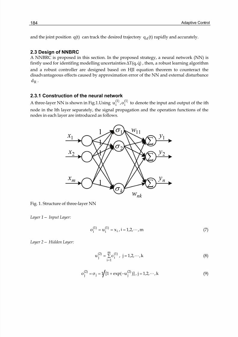
Adaptive Control184
and the joint position q(t) can track the desired trajectory (t)qd rapidly and accurately.
2.3 Design of NNBRCA NNBRC is proposed in this section. In the proposed strategy, a neural network (NN) is
firstly used for identifing modelling uncertainties )qΔT(q, & , then, a robust learning algorithm
and a robust controller are designed based on HJI equation theorem to counteract thedisadvantageous effects caused by approximation error of the NN and external disturbance
Rd .
2.3.1 Construction of the neural network
A three-layer NN is shown in Fig.1.Using(1)i
(1)i o,u to denote the input and output of the ith
node in the lth layer separately, the signal propagation and the operation functions of thenodes in each layer are introduced as follows.
1σ
2σ
k σ
1 x
2 x
m x
1 y
2 y
n y
1
1
1
1
11w
nk w
∑
∑
∑
Fig. 1. Structure of three-layer NN
Layer 1— Input Layer:
i(1)i
(1)i xuo == , m,1,2,i L= (7)
Layer 2— Hidden Layer:
∑==
m
1i
(1)i
(2) j ou , k,1,2, j L= (8)
])uexp([11σo(2) j j
(2) j −+== , k,1,2, j L= (9)
Adaptive Control Based On Neural Network 185
Layer 3— Output Layer:
∑ ⋅====
k
1 j
(2) jhj
(3)h
(3)hh owuoy , n,1,2,h L= (10)
Let
⎥⎥⎥⎥⎥
⎦
⎤
⎢⎢⎢⎢⎢
⎣
⎡
=
nkn2n1
2k2221
1k1211
www
www
www
W
L
MMMM
L
L
,
⎥⎥⎥⎥⎥
⎦
⎤
⎢⎢⎢⎢⎢
⎣
⎡
=
k
2
1
σ
σ
σ
σ M
,
⎥⎥⎥⎥⎥
⎦
⎤
⎢⎢⎢⎢⎢
⎣
⎡
=
n
2
1
y
y
y
YM
then the outputs of the three-layer NN can be written as:
σ WY = (11)
In this paper, the three-layer NN described above will be used to identify the modelinguncertainties )qΔT(q, & in robotic system. Using Tε to denote the network approximation
error, then the modeling uncertainties can be denoted by:
)qT(q,W)q(q,ΔT TTT && Δ+= ε σ (12)
where TW is the weight matrix, Tσ is the activation function vector.
Substitute (12) into (4), then the dynamics of the robot manipulator with a NN identifier canbe formulated as:
TdWG(q)q)qV(q,qM(q) RTTT =+++++ ε σ &&&& (13)
Regarding T ε as another external disturbance of robotic system, and using RTR d+= ε ε ,
then (13) can be rewritten as:
TWG(q)q)qV(q,qM(q) RTT =++++ ε σ &&&& (14)
For attenuating disadvantageous effects caused by Rε to a prescribed level, a robust
learning algorithm of NN and a robust controller can be designed based on HJI equation asbelow 2.3.2.
2.3.2 Robust controller and NN learning algorithmAt first, we introduce a control signal u, which satisfies:
TuG(q)q)qV(q,qM(q) dd =+++ &&&& (15)
where nddd Rq,q,q ∈&&& is desired joint position, velocity, and acceleration vectors separately.
Adaptive Control186
Thus, the closed-loop robot control system can be constructed by substituting (15) into (14).Let dqqe −= , the closed-loop system can be formulated as:
uWe)qV(q,eM(q) RTT =+++ ε σ &&&& (16)
By regarding Rε as external disturbance and introducing the evaluation signal pezR = ,
where p is a positive constant, we can define the index signal as:
2
2
02
sup JR
R
RR
z
ε ε ≠
= (17)
The idea of NNBRC is to design controller u and the NN learning algorithm TW& such that
R J is less than a prescribed level, γ .
Define two state variables as:
⎩⎨⎧
+=
=
eex
ex
2
1
α &(18)
where α is an prescribed positive constant. Thus, system (16) can be rewritten as:
⎩⎨⎧
+−−+−=
−=
uWVxxM
xxx
RTT22
121
ε σ ω
α
&
&(19)
where eVeMω α α += & , TW is a kn × matrix that can be described as:
[ ]TkT2T1
nkTn2Tn1T
2kT22T21T
1kT12T11T
T w w w
www
www
www
W L
L
MMMM
L
L
=
⎥⎥⎥⎥⎥
⎦
⎤
⎢⎢⎢⎢⎢
⎣
⎡
=
Theorem 1: Considering system (19), if the learning algorithm of NN is:
TT WW η −=& (20)
The controller u is designed as:
222TT1 x2Y
1Wxu ⎟⎟
⎠
⎞⎜⎜⎝
⎛ +−+−−= ε σ ω (21)
and the parameter p in the evaluation signal , 1R pxpez == , satisfies:
Adaptive Control Based On Neural Network 187
12p
2
1- ε α = (22)
where 21 ,ε ε and η are all prescribed positive constant, then the disturbance restraint index
signal of system (19), R J , is less than γ .
Proof: Considering system (19), we define the following derivable function:
2T2
T21
T1 W
2
1xMx
2
1xx
2
1L ⋅+⋅⋅⋅+⋅⋅= (23)
Thus,
( ) ( )
∑++
+−−+−=
∑+++=
=
=
m
1iTi
TTi2
T2
RTTT212
T1
m
1iiT
TiT2
T22
T21
T1
wwx)2V-M(x2
1
uWxxxx
wwxMx2
1xMxxxL
&&
&&&&&
ε σ ω α
According to Property 2 of the robot dynamics, the above equation can be rewritten as:
Ti
m
1i
TTiRTT1
T21
T1
Ti
m
1i
TTiRTT
T212
T1
wwu)-w-(xxxx
wwu)-w-(x)x-(xxL
&
&&
∑++++−=
∑+++=
=
=
ε σ ω α
ε σ ω α
Substituting (20) into above equation, then
2TRTT1
T21
T1 W-u)-W-(xxxxL η ε σ ω α +++−=&
Regarding Rε as external disturbance, let
21
22R
22T
RT2TT1
T2
21
2R
2R
2
xp2
1
2
1W
x)uWx(xx
z2
1
2
1LH
+−−
−+−++−=
+−=
ε γ η
ε σ ω α
ε γ &
( )uWxxxp2
1- TT1
T2
21
2 +−++⎟ ⎠
⎞⎜⎝
⎛ −= σ ω α
2R
22TR
T2
2
1Wx ε γ η ε −−−
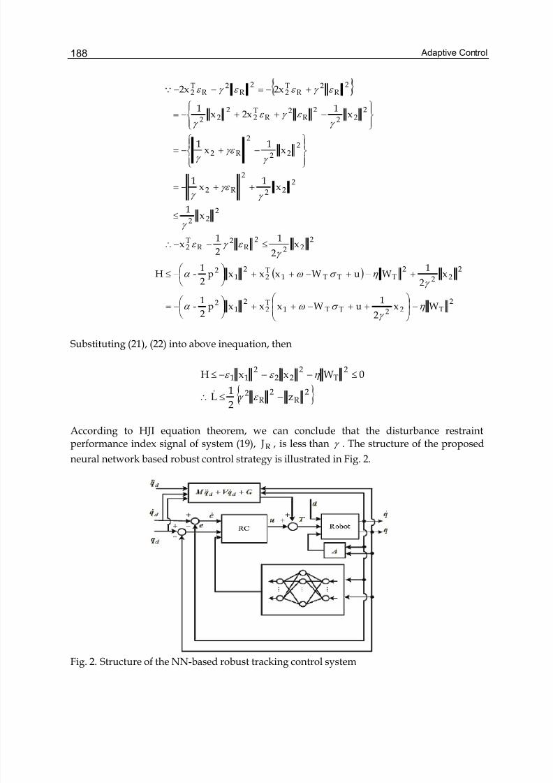
Adaptive Control188
( )
2T22TT1
T2
21
2
222
2TTT1
T2
21
2
222
2R
2R
T2
222
222
2
R2
222
2
R2
222
2R
2R
T2
222
2R
2R
T2
2R
2R
T2
Wx2
1uWxxxp
2
1-
x2
1WuWxxxp
2
1-H
x2
1
2
1x
x1
x1
x1
x1
x1
x1
2xx1
2x2x
η γ
σ ω α
γ η σ ω α
γ ε γ ε
γ
γ γε
γ
γ γε
γ
γ ε γ ε
γ
ε γ ε ε γ ε
−⎟⎟
⎠
⎞
⎜⎜
⎝
⎛ ++−++⎟
⎠
⎞⎜⎝
⎛ −=
+−+−++⎟ ⎠
⎞⎜⎝
⎛ −≤
≤−−∴
≤
++−=
⎪⎭
⎪⎬⎫
⎪⎩
⎪⎨⎧
−+−=
⎪⎭
⎪⎬⎫
⎪⎩
⎪⎨⎧
−++−=
+−=−−Q
Substituting (21), (22) into above inequation, then
2R
2R
2
2T
222
211
z2
1L
0WxxH
−≤∴
≤−−−≤
ε γ
η ε ε
&
According to HJI equation theorem, we can conclude that the disturbance restraint
performance index signal of system (19), R J , is less than γ . The structure of the proposed
neural network based robust control strategy is illustrated in Fig. 2.
Fig. 2. Structure of the NN-based robust tracking control system
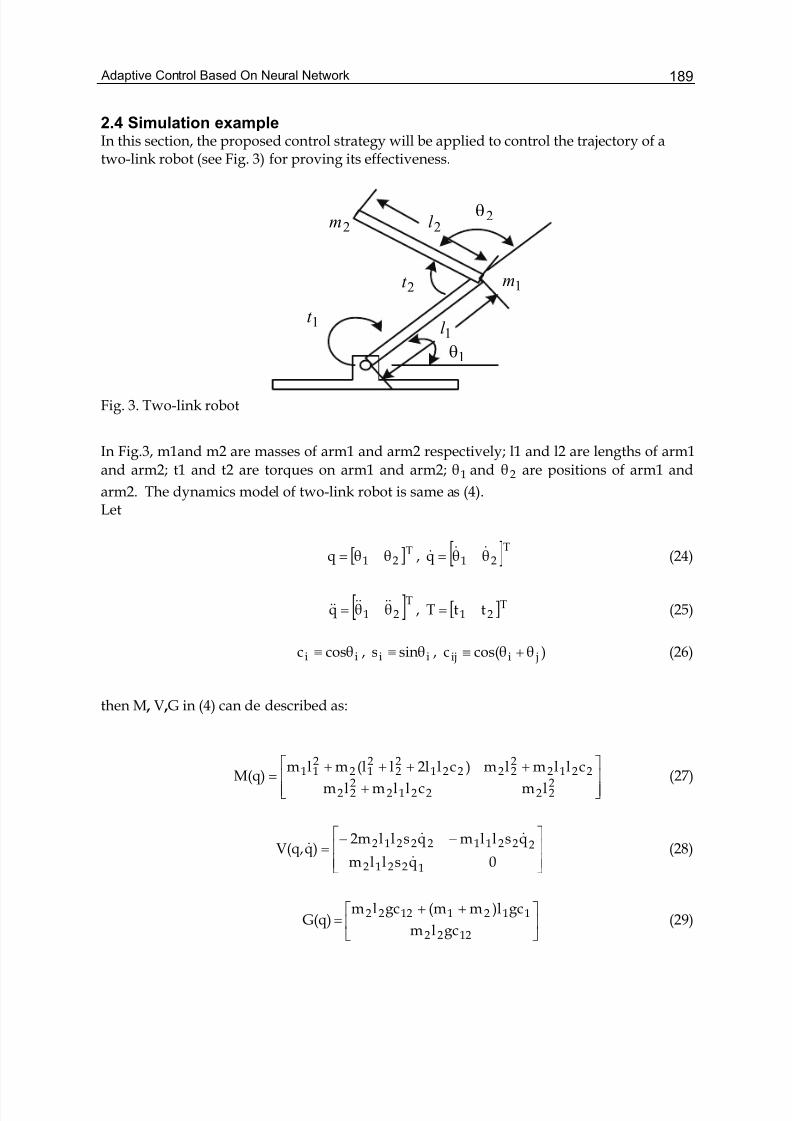
Adaptive Control Based On Neural Network 189
2.4 Simulation exampleIn this section, the proposed control strategy will be applied to control the trajectory of atwo-link robot (see Fig. 3) for proving its effectiveness.
1t
2t 1m
2m
1l
2l
1θ
2θ
Fig. 3. Two-link robot
In Fig.3, m1and m2 are masses of arm1 and arm2 respectively; l1 and l2 are lengths of arm1
and arm2; t1 and t2 are torques on arm1 and arm2; 1θ and 2θ are positions of arm1 and
arm2. The dynamics model of two-link robot is same as (4).Let
[ ]T21 θ θq = , [ ]T21 θ θq &&& = (24)
[ ]T21 θ θq &&&&&& = , [ ]T21 t tT = (25)
ii cosθc ≡ , ii sinθs ≡ , )θcos(θc jiij +≡ (26)
then M , V ,G in (4) can de described as:
⎥⎥⎦
⎤
⎢⎢⎣
⎡
+
++++=
2222212
222
2212222221
22
212
211
lmcllmlm
cllmlm)cl2ll(lmlmM(q) (27)
⎥⎥
⎦
⎤
⎢⎢
⎣
⎡ −−=
0qsllm
qsllmqsll2m)qV(q,
12212
2221122212
&
&&& (28)
⎥⎦
⎤⎢⎣
⎡ ++=
1222
11211222
gclm
gc)lm(mgclmG(q) (29)
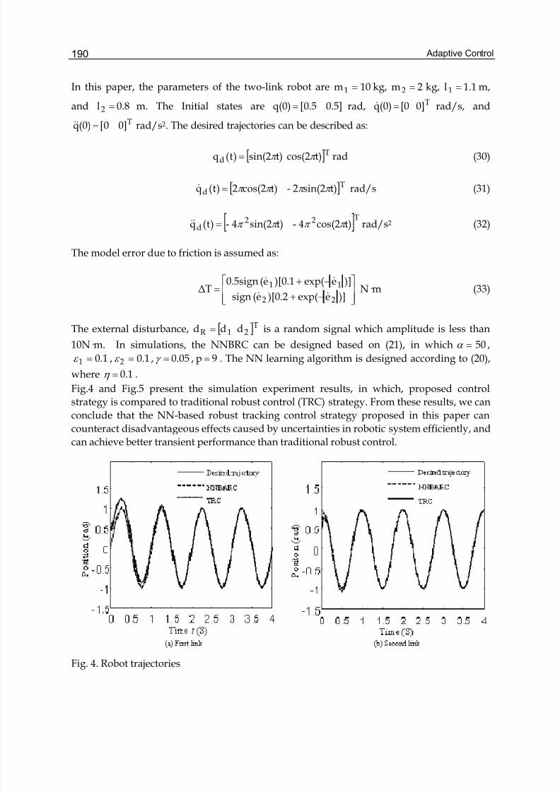
Adaptive Control190
In this paper, the parameters of the two-link robot are 10m1 = kg, 2m 2 = kg, 1.1l1 = m,
and 0.8l2 = m. The Initial states are 0.5]0.5[q(0) = rad, T0] [0(0)q =& rad/s, and
T0]0[(0)q =&& rad/s2. The desired trajectories can be described as:
[ ]Td t)cos(2 t)sin(2)t(q π π = rad (30)
[ ]Td t)sin(22- t)cos(22)t(q π π π π =& rad/s (31)
[ ]T22d t)cos(24- t)sin(24-)t(q π π π π =&& rad/s2 (32)
The model error due to friction is assumed as:
⎥⎥⎦
⎤
⎢⎢⎣
⎡
−+
−+=
)]eexp()[0.2e(sign
)]eexp()[0.1e(0.5signΔT
22
11
&&
&&N·m (33)
The external disturbance, [ ]T21R d dd = is a random signal which amplitude is less than
10N·m. In simulations, the NNBRC can be designed based on (21), in which 50=α ,
0.11 =ε , 0.12 =ε , 0.05=γ , 9p = . The NN learning algorithm is designed according to (20),
where 0.1=η .
Fig.4 and Fig.5 present the simulation experiment results, in which, proposed control
strategy is compared to traditional robust control (TRC) strategy. From these results, we can
conclude that the NN-based robust tracking control strategy proposed in this paper can
counteract disadvantageous effects caused by uncertainties in robotic system efficiently, and
can achieve better transient performance than traditional robust control.
Fig. 4. Robot trajectories
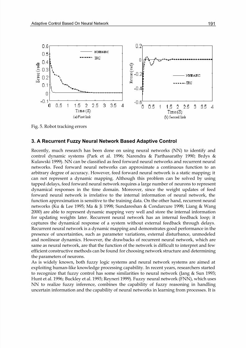
Adaptive Control Based On Neural Network 191
Fig. 5. Robot tracking errors
3. A Recurrent Fuzzy Neural Network Based Adaptive Control
Recently, much research has been done on using neural networks (NN) to identify andcontrol dynamic systems (Park et al. 1996; Narendra & Parthasarathy 1990; Brdys &Kulawski 1999). NN can be classified as feed forward neural networks and recurrent neuralnetworks. Feed forward neural networks can approximate a continuous function to anarbitrary degree of accuracy. However, feed forward neural network is a static mapping; itcan not represent a dynamic mapping. Although this problem can be solved by usingtapped delays, feed forward neural network requires a large number of neurons to representdynamical responses in the time domain. Moreover, since the weight updates of feedforward neural network is irrelative to the internal information of neural network, thefunction approximation is sensitive to the training data. On the other hand, recurrent neuralnetworks (Ku & Lee 1995; Ma & Ji 1998; Sundareshan & Condarcure 1998; Liang & Wang2000) are able to represent dynamic mapping very well and store the internal informationfor updating weights later. Recurrent neural network has an internal feedback loop; itcaptures the dynamical response of a system without external feedback through delays.Recurrent neural network is a dynamic mapping and demonstrates good performance in thepresence of uncertainties, such as parameter variations, external disturbance, unmodeledand nonlinear dynamics. However, the drawbacks of recurrent neural network, which aresame as neural network, are that the function of the network is difficult to interpret and fewefficient constructive methods can be found for choosing network structure and determiningthe parameters of neurons.As is widely known, both fuzzy logic systems and neural network systems are aimed atexploiting human-like knowledge processing capability. In recent years, researchers startedto recognize that fuzzy control has some similarities to neural network (Jang & Sun 1993;Hunt et al. 1996; Buckley et al. 1993; Reyneri 1999). Fuzzy neural network (FNN), which usesNN to realize fuzzy inference, combines the capability of fuzzy reasoning in handlinguncertain information and the capability of neural networks in learning from processes. It is
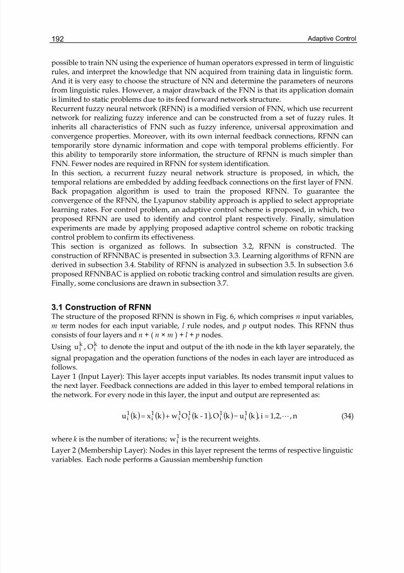
Adaptive Control192
possible to train NN using the experience of human operators expressed in term of linguisticrules, and interpret the knowledge that NN acquired from training data in linguistic form.And it is very easy to choose the structure of NN and determine the parameters of neuronsfrom linguistic rules. However, a major drawback of the FNN is that its application domainis limited to static problems due to its feed forward network structure.Recurrent fuzzy neural network (RFNN) is a modified version of FNN, which use recurrentnetwork for realizing fuzzy inference and can be constructed from a set of fuzzy rules. Itinherits all characteristics of FNN such as fuzzy inference, universal approximation andconvergence properties. Moreover, with its own internal feedback connections, RFNN cantemporarily store dynamic information and cope with temporal problems efficiently. Forthis ability to temporarily store information, the structure of RFNN is much simpler thanFNN. Fewer nodes are required in RFNN for system identification.In this section, a recurrent fuzzy neural network structure is proposed, in which, thetemporal relations are embedded by adding feedback connections on the first layer of FNN.Back propagation algorithm is used to train the proposed RFNN. To guarantee theconvergence of the RFNN, the Lyapunov stability approach is applied to select appropriatelearning rates. For control problem, an adaptive control scheme is proposed, in which, twoproposed RFNN are used to identify and control plant respectively. Finally, simulationexperiments are made by applying proposed adaptive control scheme on robotic trackingcontrol problem to confirm its effectiveness.This section is organized as follows. In subsection 3.2, RFNN is constructed. Theconstruction of RFNNBAC is presented in subsection 3.3. Learning algorithms of RFNN arederived in subsection 3.4. Stability of RFNN is analyzed in subsection 3.5. In subsection 3.6proposed RFNNBAC is applied on robotic tracking control and simulation results are given.Finally, some conclusions are drawn in subsection 3.7.
3.1 Construction of RFNNThe structure of the proposed RFNN is shown in Fig. 6, which comprises n input variables,m term nodes for each input variable, l rule nodes, and p output nodes. This RFNN thusconsists of four layers and n + ( n × m ) + l + p nodes.
Using kiu , k
iO to denote the input and output of the ith node in the kth layer separately, the
signal propagation and the operation functions of the nodes in each layer are introduced asfollows.Layer 1 (Input Layer): This layer accepts input variables. Its nodes transmit input values tothe next layer. Feedback connections are added in this layer to embed temporal relations inthe network. For every node in this layer, the input and output are represented as:
( ) ( ) ( ) ( ) ( ) n,1,2,i,kukO,1-kOwkxku 1i
1i
1i
1i
1i
1i L==+= (34)
where k is the number of iterations; 1iw is the recurrent weights.
Layer 2 (Membership Layer): Nodes in this layer represent the terms of respective linguisticvariables. Each node performs a Gaussian membership function
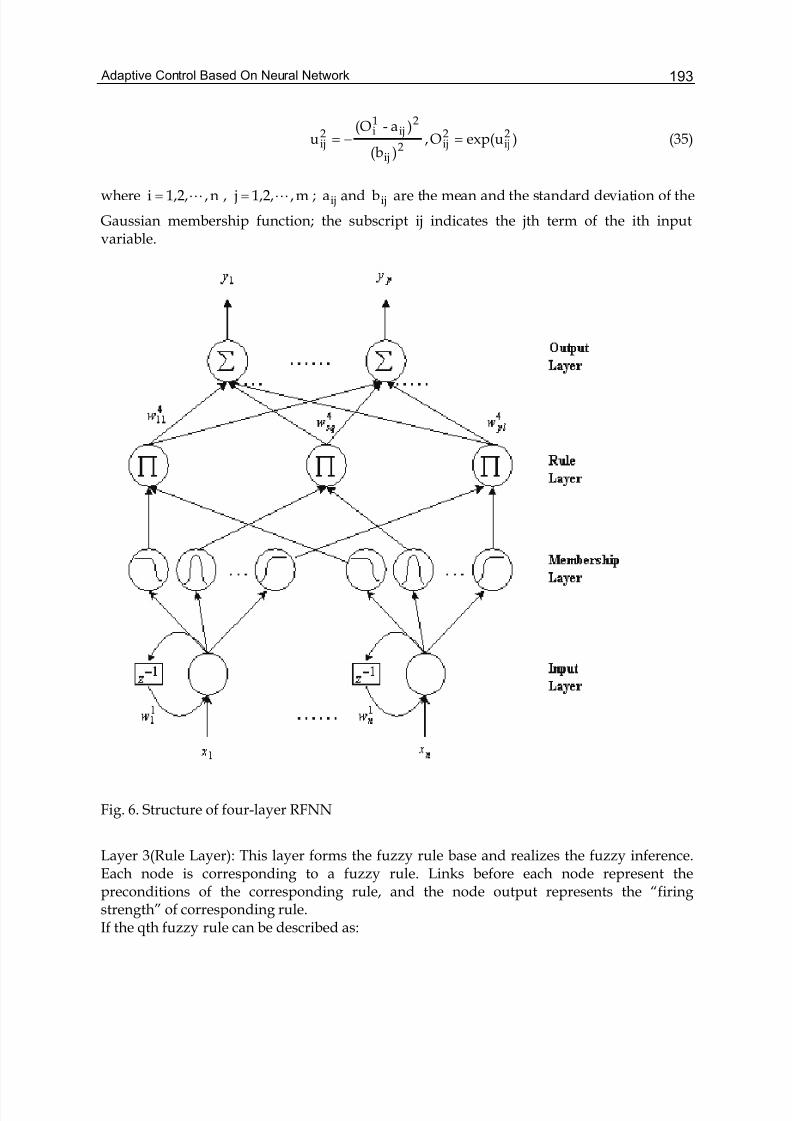
Adaptive Control Based On Neural Network 193
)exp(uO,)(b
)a-(Ou 2
ij2ij2
ij
2ij
1i2
ij =−= (35)
where n,1,2,i L= , m,1,2, j L= ; ija and ijb are the mean and the standard deviation of the
Gaussian membership function; the subscript ij indicates the jth term of the ith inputvariable.
Fig. 6. Structure of four-layer RFNN
Layer 3(Rule Layer): This layer forms the fuzzy rule base and realizes the fuzzy inference.Each node is corresponding to a fuzzy rule. Links before each node represent thepreconditions of the corresponding rule, and the node output represents the “firingstrength” of corresponding rule.If the qth fuzzy rule can be described as:
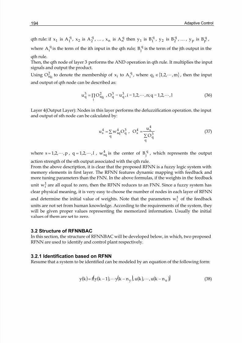
Adaptive Control194
qth rule: if 1x isq
1A , 2x isq2A , … , nx is q
nA then 1y is q1B , 2y is q
2B , … , py is qpB ,
whereq
iA is the term of the ith input in the qth rule; q jB is the term of the jth output in the
qth rule.Then, the qth node of layer 3 performs the AND operation in qth rule. It multiplies the inputsignals and output the product.
Using 2iiqO to denote the membership of ix to
qiA , where m,1,2,qi L∈ , then the input
and output of qth node can be described as:
∏=i
2iiq
3q Ou , l,1,2,qn;,1,2,i,uO 3
q3q LL === (36)
Layer 4(Output Layer): Nodes in this layer performs the defuzzification operation. the inputand output of sth node can be calculated by:
∑=q
3q
4sq
4s Owu ,
∑=
q
3q
4s4
sO
uO (37)
where p,1,2,s L= , l,1,2,q L= , 4sqw is the center of q
jB , which represents the output
action strength of the sth output associated with the qth rule.From the above description, it is clear that the proposed RFNN is a fuzzy logic system withmemory elements in first layer. The RFNN features dynamic mapping with feedback andmore tuning parameters than the FNN. In the above formulas, if the weights in the feedback
unit 1iw are all equal to zero, then the RFNN reduces to an FNN. Since a fuzzy system has
clear physical meaning, it is very easy to choose the number of nodes in each layer of RFNN
and determine the initial value of weights. Note that the parameters 1iw of the feedback
units are not set from human knowledge. According to the requirements of the system, theywill be given proper values representing the memorized information. Usually the initialvalues of them are set to zero.
3.2 Structure of RFNNBACIn this section, the structure of RFNNBAC will be developed below, in which, two proposedRFNN are used to identify and control plant respectively.
3.2.1 Identification based on RFNNResume that a system to be identified can be modeled by an equation of the following form:
( ) ( ) ( ) ( )uy nku,,ku,nky,1kyfky −−−= LL (38)
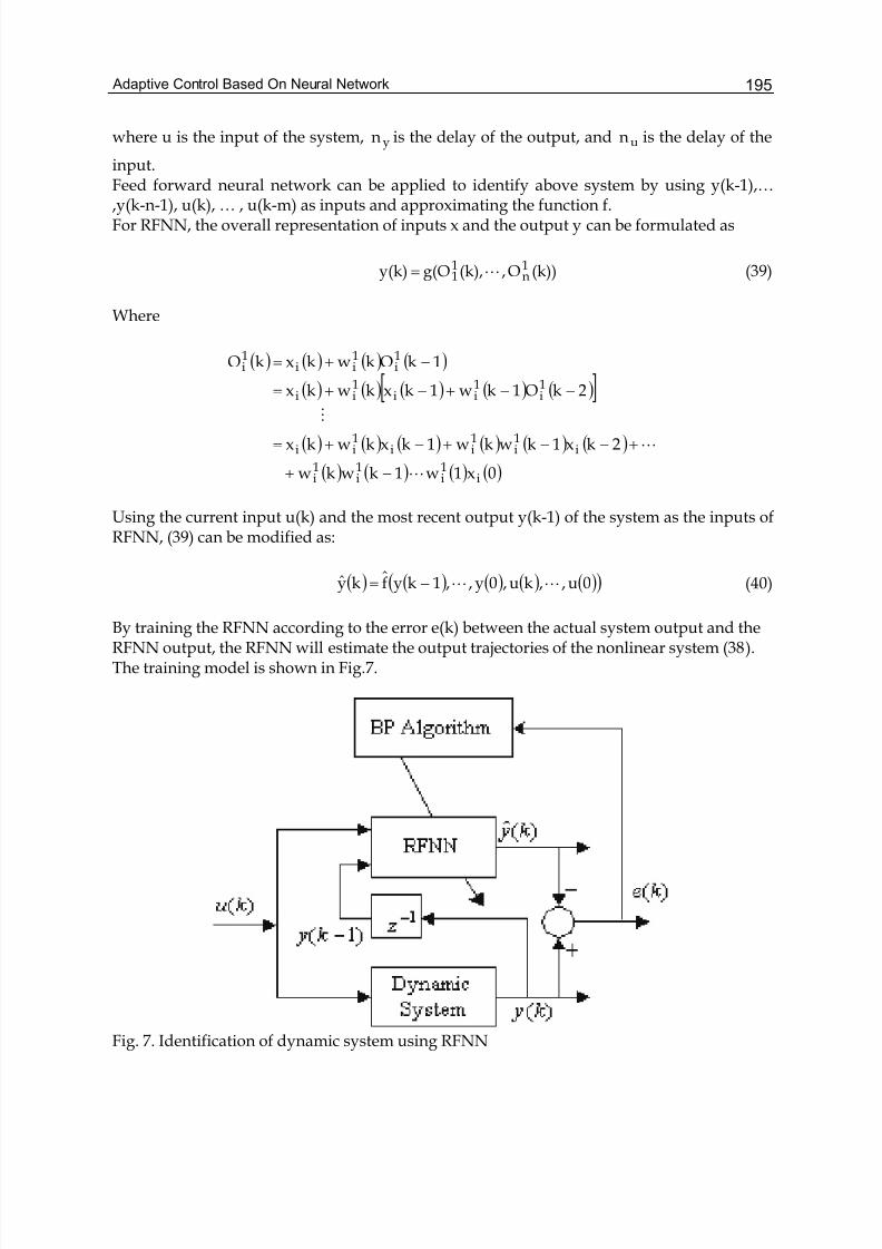
Adaptive Control Based On Neural Network 195
where u is the input of the system, yn is the delay of the output, and un is the delay of the
input.Feed forward neural network can be applied to identify above system by using y(k-1),…,y(k-n-1), u(k), … , u(k-m) as inputs and approximating the function f.For RFNN, the overall representation of inputs x and the output y can be formulated as
(k))O,(k),g(Oy(k) 1n
11 L= (39)
Where
( ) ( ) ( ) ( )
( ) ( ) ( ) ( ) ( )[ ]
( ) ( ) ( ) ( ) ( ) ( )
( ) ( ) ( ) ( )0x1w1kwkw
2kx1kwkw1kxkwkx
2kO1kw1kxkwkx
1kOkwkxkO
i1i
1i
1i
i1i
1ii
1ii
1i
1ii
1ii
1i
1ii
1i
L
L
M
−+
+−−+−+=
−−+−+=
−+=
Using the current input u(k) and the most recent output y(k-1) of the system as the inputs ofRFNN, (39) can be modified as:
( ) ( ) ( ) ( ) ( )( )0u,,ku,0y,,1kyfky LL−= (40)
By training the RFNN according to the error e(k) between the actual system output and theRFNN output, the RFNN will estimate the output trajectories of the nonlinear system (38).The training model is shown in Fig.7.
Fig. 7. Identification of dynamic system using RFNN
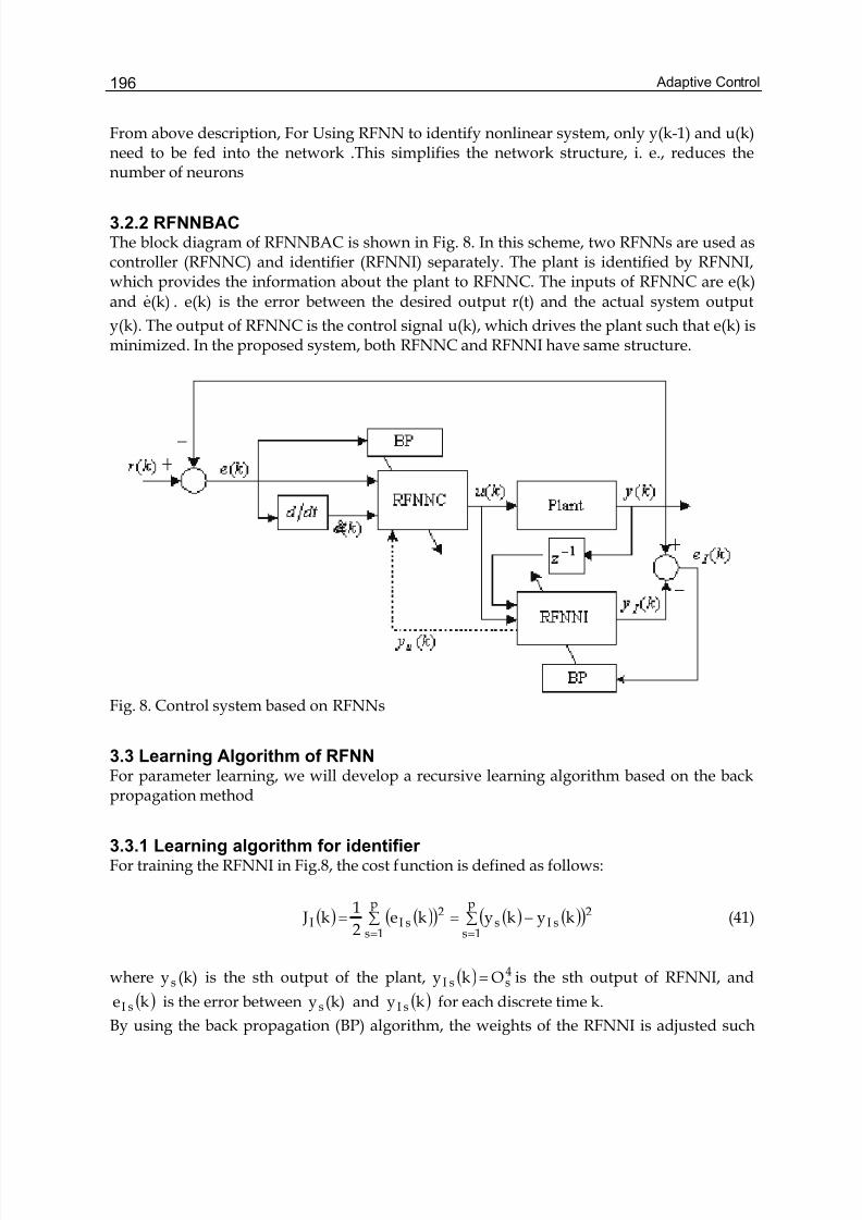
Adaptive Control196
From above description, For Using RFNN to identify nonlinear system, only y(k-1) and u(k)need to be fed into the network .This simplifies the network structure, i. e., reduces thenumber of neurons
3.2.2 RFNNBACThe block diagram of RFNNBAC is shown in Fig. 8. In this scheme, two RFNNs are used ascontroller (RFNNC) and identifier (RFNNI) separately. The plant is identified by RFNNI,which provides the information about the plant to RFNNC. The inputs of RFNNC are e(k)and (k)e& . e(k) is the error between the desired output r(t) and the actual system output
y(k). The output of RFNNC is the control signal u(k), which drives the plant such that e(k) isminimized. In the proposed system, both RFNNC and RFNNI have same structure.
Fig. 8. Control system based on RFNNs
3.3 Learning Algorithm of RFNNFor parameter learning, we will develop a recursive learning algorithm based on the backpropagation method
3.3.1 Learning algorithm for identifier For training the RFNNI in Fig.8, the cost function is defined as follows:
( ) ( )( ) ( ) ( )( )∑ ∑ −=== =
p
1s
p
1s
2sIs
2sII kykyke
2
1k J (41)
where (k)ys is the sth output of the plant, ( ) 4ssI Oky = is the sth output of RFNNI, and
( )ke sI is the error between (k)ys and ( )ky sI for each discrete time k.
By using the back propagation (BP) algorithm, the weights of the RFNNI is adjusted such
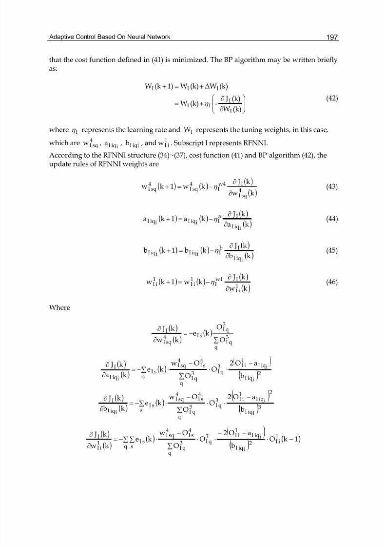
Adaptive Control Based On Neural Network 197
that the cost function defined in (41) is minimized. The BP algorithm may be written brieflyas:
⎟⎟ ⎠
⎞⎜⎜⎝
⎛
∂
∂+=
+=+
(k)W
(k) J-(k)W
(k)ΔW(k)W1)(kW
I
III
III
η (42)
where Iη represents the learning rate and IW represents the tuning weights, in this case,
which are 4sqIw ,
iiqIa , iqiIb , and 1iIw . Subscript I represents RFNNI.
According to the RFNNI structure (34)~(37), cost function (41) and BP algorithm (42), theupdate rules of RFNNI weights are
( ) ( )( )
( )kw
k Jkw1kw
4sqI
Iw4I
4sqI
4sqI
∂
∂−=+ η (43)
( ) ( )( )
( )ka
k Jka1ka
iiqI
IaIiiqIiiqI∂
∂−=+ η (44)
( ) ( )( )
( )kb
k Jkb1kb
iiqI
IbIiiqIiiqI∂
∂−=+ η (45)
( ) ( )( )
( )kw
k Jkw1kw
1iI
Iw1I
1iI
1iI
∂
∂−=+ η (46)
Where
( )
( )( )∑
−=∂
∂
q
3qI
3qI
sI4sqI
I
O
Oke
kw
k J
( )( )
( )( )
∑−
⋅⋅∑
−⋅−=
∂
∂
s2
iiqI
iiqI1
iI3qI
q
3qI
4sI
4sqI
sIiiqI
I
b
aO2O
O
Owke
ka
k J
( )( )
( )( )
( )∑
−⋅⋅
∑
−⋅−=
∂
∂
s3
iiqI
2
iiqI1
iI3qI
q
3qI
4sI
4sqI
sIiiqI
I
b
aO2O
O
Owke
kb
k J
( )
( )( )
)( )
( )1kOb
aO2O
O
Owke
kw
k J 1iI2
iiqI
iiqI1
iI3qI
q sq
3qI
4sI
4sqI
sI1iI
I −⋅−−
⋅⋅∑∑∑
−⋅−=
∂
∂
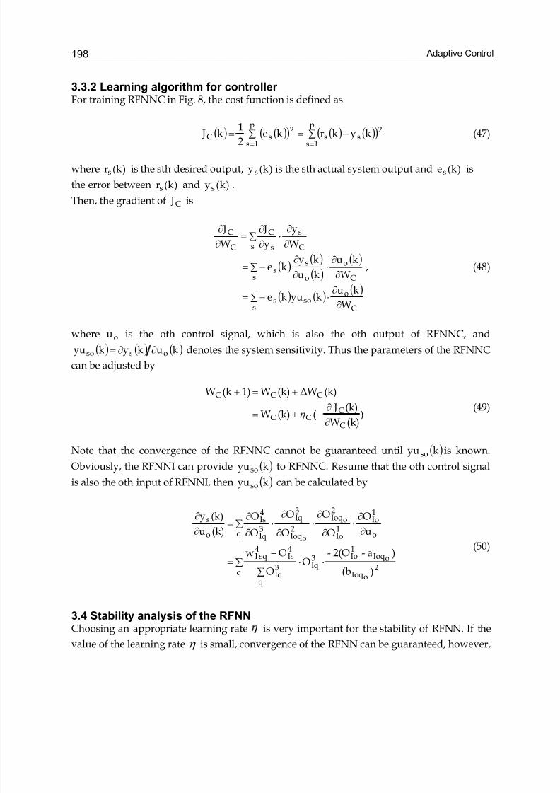
Adaptive Control198
3.3.2 Learning algorithm for controller For training RFNNC in Fig. 8, the cost function is defined as
( ) ( )( ) ( ) ( )( )∑ ∑ −=== =
p
1s
p
1s
2ss
2sC kykrke
2
1k J (47)
where )k(rs is the sth desired output, )k(ys is the sth actual system output and )k(es is
the error between )k(rs and )k(ys .
Then, the gradient of C J is
( )( )( )
( )
( ) ( )( )
∑∂
∂⋅−=
∑∂
∂⋅
∂
∂−=
∑∂
∂⋅
∂
∂=
∂
∂
s C
osos
s C
o
o
ss
s C
s
s
C
C
C
W
kukyuke
W
ku
ku
kyke
W
y
y
J
W
J
, (48)
where ou is the oth control signal, which is also the oth output of RFNNC, and
( ) ( ) ( )kukykyu osso ∂∂= denotes the system sensitivity. Thus the parameters of the RFNNC
can be adjusted by
)(k)W
(k) J((k)W
(k)ΔW(k)W1)(kW
C
CCC
CCC
∂
∂−+=
+=+
η (49)
Note that the convergence of the RFNNC cannot be guaranteed until ( )kyuso is known.
Obviously, the RFNNI can provide ( )kyuso to RFNNC. Resume that the oth control signal
is also the oth input of RFNNI, then ( )kyuso can be calculated by
2oIoq
oIoq1Io3
Iqq
q
3Iq
4Is
4sqI
o
1Io
1Io
2oIoq
2oIoq
3Iq
q3Iq
4Is
o
s
)(b
)a-2(O- O
O
Ow
u
O
O
O
O
O
O
O
(k)u
(k)y
⋅∑ ⋅∑
−=
∂
∂⋅
∂
∂⋅
∂
∂⋅∑
∂
∂=
∂
∂
(50)
3.4 Stability analysis of the RFNNChoosing an appropriate learning rate is very important for the stability of RFNN. If the
value of the learning rate η is small, convergence of the RFNN can be guaranteed, however,
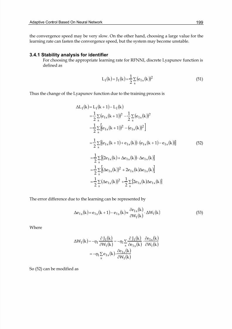
Adaptive Control Based On Neural Network 199
the convergence speed may be very slow. On the other hand, choosing a large value for thelearning rate can fasten the convergence speed, but the system may become unstable.
3.4.1 Stability analysis for identifier For choosing the appropriate learning rate for RFNNI, discrete Lyapunov function isdefined as
( ) ( ) ( )( )∑==s
2sIII ke
2
1k JkL (51)
Thus the change of the Lyapunov function due to the training process is
( ) ( ) ( )
( )( ) ( )( )
( )( ) ( )( )[ ]∑ −+=
∑ ∑−+=
−+=
s
2sI
2sI
s s
2sI
2sI
III
ke1ke2
1
ke2
11ke
2
1
kL1kLkΔL
( ) ( )( ) ( ) ( )( )[ ]∑ −+⋅++=s
sIsIsIsI ke1keke1ke2
1(52)
( ) ( )( ) ( )[ ]
( )( ) ( ) ( )[ ]
( )( ) ( ) ( )[ ]∑∑ +=
∑ +=
∑ ⋅+=
ssIsI
s
2sI
ssIsI
2sI
ssIsIsI
kΔek2e2
1kΔe
2
1
kΔek2ekΔe2
1
kΔekΔek2e2
1
The error difference due to the learning can be represented by
( ) ( ) ( )( )( )
( )kΔWkW
ke ke1kekΔe I
I
sIsIsIsI ⋅
∂
∂≈−+= (53)
Where
( )( )( )
( )( )
( )( )
( )( )( )kW
keke
kW
ke
ke
k J
kW
k JkΔW
I
sI
ssII
s I
sI
sI
II
I
III
∂
∂∑ ⋅−=
∑∂
∂⋅
∂
∂−=
∂
∂−=
η
η η
So (52) can be modified as
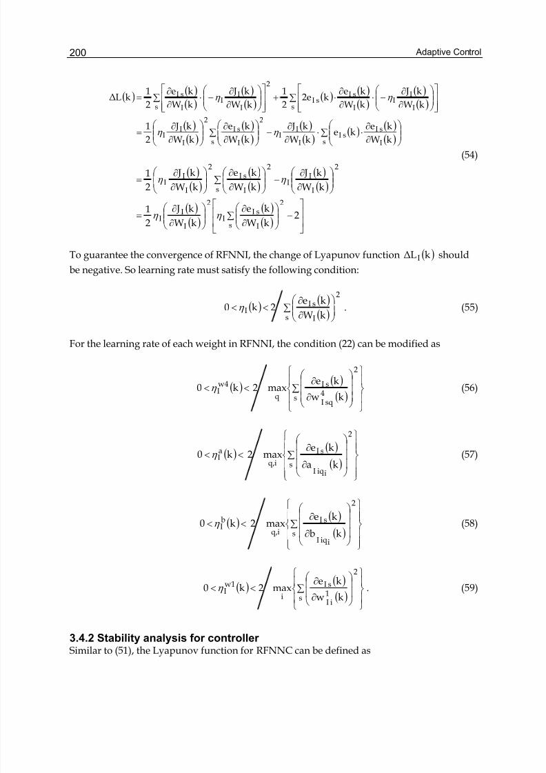
Adaptive Control200
( )( )( )
( )( )
( )( )( )
( )( )
( )( )
( )( )
( )( )
( )( )( )
∑ ⎟⎟ ⎠
⎞⎜⎜⎝
⎛
∂
∂⋅⋅
∂
∂−∑ ⎟
⎟ ⎠
⎞⎜⎜⎝
⎛
∂
∂⎟⎟ ⎠
⎞⎜⎜⎝
⎛
∂
∂=
∑⎥⎥⎦
⎤
⎢⎢⎣
⎡⎟⎟ ⎠
⎞⎜⎜⎝
⎛
∂
∂−⋅
∂
∂⋅+∑
⎥⎥⎦
⎤
⎢⎢⎣
⎡⎟⎟ ⎠
⎞⎜⎜⎝
⎛
∂
∂−⋅
∂
∂=
s I
sIsI
I
II
2
s I
sI2
I
II
s I
II
I
sIsI
2
s I
II
I
sI
kW
keke
kW
k J
kW
ke
kW
k J
2
1
kW
k J
kW
kek2e
2
1
kW
k J
kW
ke
2
1kΔL
η η
η η
(54)
( )( )
( )( )
( )( )
( )( )
( )( ) ⎥
⎥
⎦
⎤
⎢⎢
⎣
⎡−∑ ⎟
⎟ ⎠
⎞⎜⎜⎝
⎛
∂
∂⎟⎟ ⎠
⎞⎜⎜⎝
⎛
∂
∂=
⎟⎟ ⎠
⎞⎜⎜⎝
⎛
∂
∂−∑ ⎟
⎟ ⎠
⎞⎜⎜⎝
⎛
∂
∂⎟⎟ ⎠
⎞⎜⎜⎝
⎛
∂
∂=
2kW
ke
kW
k J
2
1
kW
k J
kW
ke
kW
k J
2
1
2
s I
sII
2
I
II
2
I
II
2
s I
sI2
I
II
η η
η η
To guarantee the convergence of RFNNI, the change of Lyapunov function ( )kΔLI should
be negative. So learning rate must satisfy the following condition:
( )( )( )
∑ ⎟⎟ ⎠
⎞⎜⎜⎝
⎛
∂
∂<<
s
2
I
sII
kW
ke2k0 η . (55)
For the learning rate of each weight in RFNNI, the condition (22) can be modified as
( )( )
( ) ⎪⎭
⎪⎬
⎫
⎪⎩
⎪⎨
⎧
∑⎟⎟⎟
⎠
⎞
⎜⎜⎜
⎝
⎛
∂
∂<<
s
2
4sqI
sI
q
w4I
kw
kemax2k0 η (56)
( )( )
( )⎪⎪⎭
⎪⎪⎬
⎫
⎪⎪⎩
⎪⎪⎨
⎧
∑⎟⎟⎟
⎠
⎞
⎜⎜⎜
⎝
⎛
∂
∂<<
s
2
iiqI
sI
iq,
aI
ka
kemax2k0 η (57)
( )( )
( )⎪⎪⎭
⎪⎪⎬
⎫
⎪⎪⎩
⎪⎪⎨
⎧
∑⎟⎟⎟
⎠
⎞
⎜⎜⎜
⎝
⎛
∂
∂<<
s
2
iiqI
sI
iq,
bI
kb
kemax2k0 η (58)
( )( )
( ) ⎪⎭
⎪⎬
⎫
⎪⎩
⎪⎨
⎧
∑ ⎟⎟
⎠
⎞
⎜⎜
⎝
⎛
∂
∂<<
s
2
1iI
sI
i
w1I
kw
kemax2k0 η . (59)
3.4.2 Stability analysis for controller Similar to (51), the Lyapunov function for RFNNC can be defined as
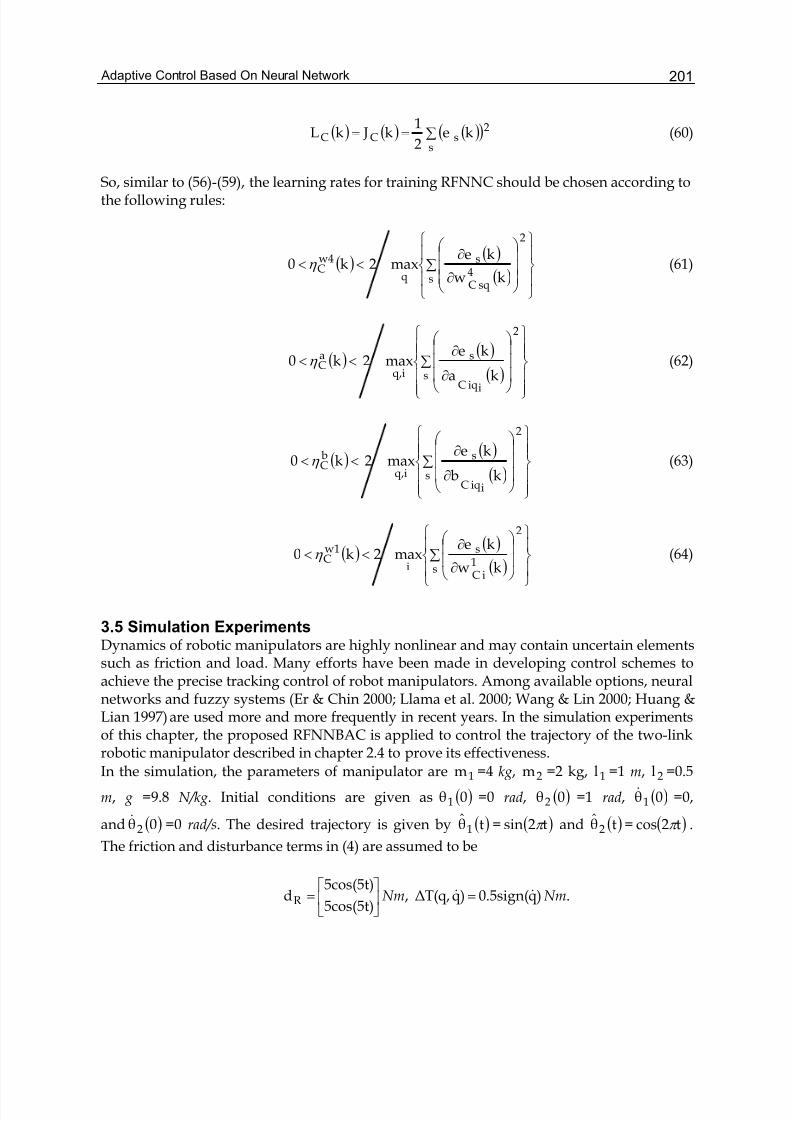
Adaptive Control Based On Neural Network 201
( ) ( ) ( )( )∑==s
2sCC ke
2
1k JkL (60)
So, similar to (56)-(59), the learning rates for training RFNNC should be chosen according tothe following rules:
( )( )
( ) ⎪⎭
⎪⎬
⎫
⎪⎩
⎪⎨
⎧
∑⎟⎟⎟
⎠
⎞
⎜⎜⎜
⎝
⎛
∂
∂<<
s
2
4sqC
s
q
w4C
kw
kemax2k0 η (61)
( )( )
( )⎪⎪⎭
⎪⎪⎬
⎫
⎪⎪⎩
⎪⎪⎨
⎧
∑⎟⎟⎟
⎠
⎞
⎜⎜⎜
⎝
⎛
∂
∂<<
s
2
iiqC
s
iq,
aC
ka
kemax2k0 η (62)
( )( )
( )⎪⎪⎭
⎪⎪⎬
⎫
⎪⎪⎩
⎪⎪⎨
⎧
∑⎟⎟⎟
⎠
⎞
⎜⎜⎜
⎝
⎛
∂
∂<<
s
2
iiqC
s
iq,
bC
kb
kemax2k0 η (63)
( )( )
( ) ⎪⎭
⎪⎬
⎫
⎪⎩
⎪⎨
⎧
∑ ⎟⎟
⎠
⎞
⎜⎜
⎝
⎛
∂
∂<<
s
2
1iC
s
i
w1C
kw
kemax2k0 η (64)
3.5 Simulation ExperimentsDynamics of robotic manipulators are highly nonlinear and may contain uncertain elementssuch as friction and load. Many efforts have been made in developing control schemes toachieve the precise tracking control of robot manipulators. Among available options, neuralnetworks and fuzzy systems (Er & Chin 2000; Llama et al. 2000; Wang & Lin 2000; Huang &Lian 1997) are used more and more frequently in recent years. In the simulation experimentsof this chapter, the proposed RFNNBAC is applied to control the trajectory of the two-linkrobotic manipulator described in chapter 2.4 to prove its effectiveness.
In the simulation, the parameters of manipulator are 1m =4 kg, 2m =2 kg, 1l =1 m, 2l =0.5
m, g =9.8 N/kg. Initial conditions are given as ( )0θ1 =0 rad, ( )0θ2 =1 rad, ( )0θ1& =0,
and ( )0θ2& =0 rad/s. The desired trajectory is given by ( )tθ1 = ( )t2sin π and ( )tθ2 = ( )t2cos π .
The friction and disturbance terms in (4) are assumed to be
⎥⎦
⎤⎢⎣
⎡=
5cos(5t)
5cos(5t)dR Nm, )q0.5sign()qΔT(q, && = Nm.
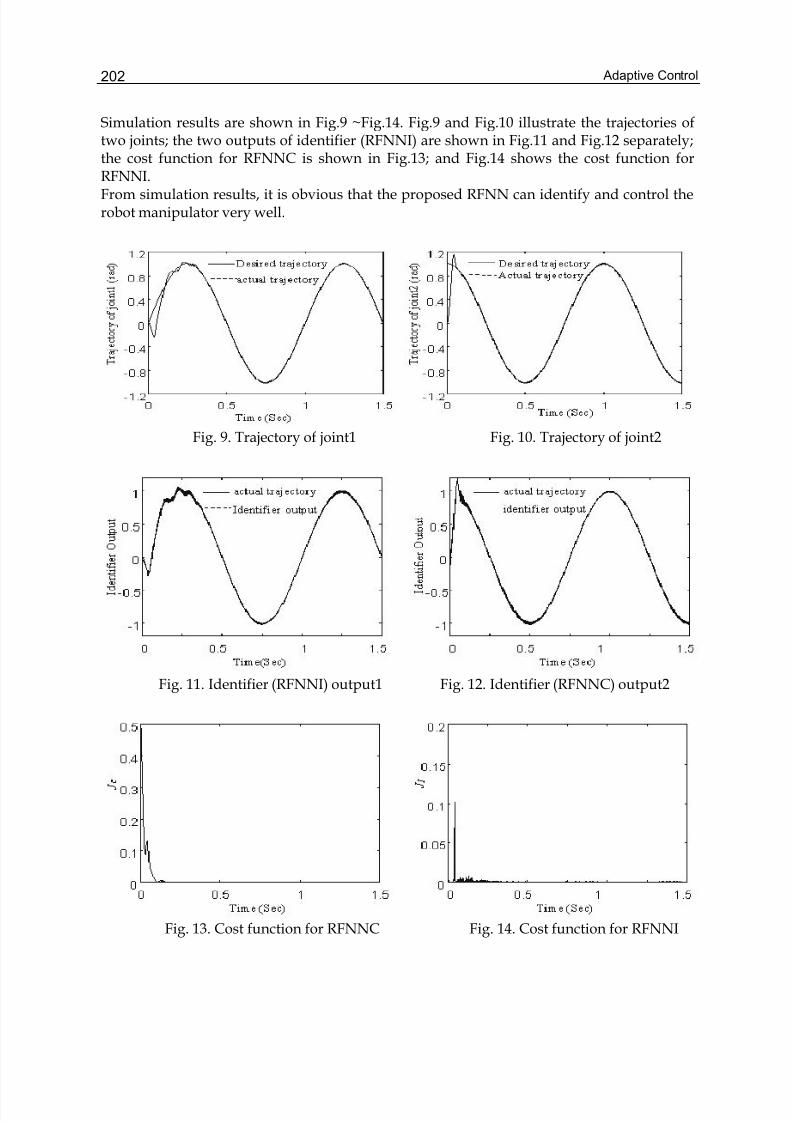
Adaptive Control202
Simulation results are shown in Fig.9 ~Fig.14. Fig.9 and Fig.10 illustrate the trajectories oftwo joints; the two outputs of identifier (RFNNI) are shown in Fig.11 and Fig.12 separately;the cost function for RFNNC is shown in Fig.13; and Fig.14 shows the cost function forRFNNI.From simulation results, it is obvious that the proposed RFNN can identify and control therobot manipulator very well.
Fig. 9. Trajectory of joint1 Fig. 10. Trajectory of joint2
Fig. 11. Identifier (RFNNI) output1 Fig. 12. Identifier (RFNNC) output2
Fig. 13. Cost function for RFNNC Fig. 14. Cost function for RFNNI
Adaptive Control Based On Neural Network 203
4. Conclusion
In this paper, the adaptive control based on neural network is studied. Firstly, a neuralnetwork based adaptive robust tracking control design is proposed for robotic systemsunder the existence of uncertainties. In this proposed control strategy, the NN is used toidentify the modeling uncertainties, and then the disadvantageous effects caused by neuralnetwork approximating error and external disturbances in robotic system are counteractedby robust controller. Especially the proposed control strategy is designed based on HJIinequation theorem to overcome the approximation error of the neural network boundedissue. Simulation results show that proposed control strategy is effective and has betterperformance than traditional robust control strategy. Secondly, an RFNN for realizing fuzzyinference using the dynamic fuzzy rules is proposed. The proposed RFNN consists of fourlayers and the feedback connections are added in first layer. The proposed RFNN can beused for the identification and control of dynamic system. For identification, RFNN onlyneeds the current inputs and most recent outputs of system as its inputs. For control, twoRFNNs are used to constitute an adaptive control system, one is used as identifier (RFNNI)and another is used as controller (RFNNC). Also to prove the proposed RFNN and controlstrategy robust, it is used to control the robot manipulator and simulation results verifiedtheir effectiveness.
5. References
Abdallah, C., Dawson, D., Dorato, P. & Jamshidi, M. (1991). Survey of the robust of rigidrobots, IEEE Control Systems Magazine, Vol. 11, No. 2, pp. 24-30.
Ortega, R. & Spong, M. W. (1989). Adaptive motion control of rigid robots: a tutorial, Automatica, Vol. 25, No. 3, pp. 877-888.
Saad, M., Dessaint, L. A., Bigras, P. & Haddad, K. (1994). Adaptive versus neural adaptivecontrol: application to robotics, International Journal of Adaptive Control and SignalProcessing, Vol. 8, No. 2, pp. 223-236.
Sanner, R. M. & Slotine, J. J. E. (1992). Gaussian networks for direct adaptive control, IEEETransactions on. Neural Network, Vol. 3, No. 4, pp. 837-863.
Spooner, J. T. & Passino, K. M. (1996). Stable adaptive control using fuzzy systems andneural networks, IEEE Transactions on Fuzzy system, Vol. 4, No. 2, pp. 339-359.
Narenra, K. S. & Parthasarathy, K. (1990). Identification and control of dynamical systemsusing neural networks, IEEE Transactions on Neural networks, Vol. 1, No. 1, pp. 4-27.
Polycarpou, M. M. (1996). Stable adaptive neural control scheme for nonlinear systems, IEEETransactions on Automatic Control, Vol. 41, No. 2, pp. 447-451.
Carelli, R., Camacho, E. F. & Patino, D. (1995). A neural network based feedforwardadaptive controller for robot, IEEE Transactions on Systems, Mman and Cybernetics,Part B: Cybernetics, Vol. 25, No. 6, pp. 1281-1288.
Behera, L., Chaudhury, S. & Gopal, M. (1996). Neuro-adaptive hybrid controller for robot-manipulator tracking control, IEE Proceedings Control Theory Applications, Vol.143,No.1, pp.2710-275.
Shen, T. L. (1996). H ∞ control theory and its applications, ISBN 7302022151, Tsinghua Press,Beijin, China.
Adaptive Control204
Park, Y. M., Choi, M. S. & Lee, K. Y. (1996). An optimal tracking neuro-controller fornonlinear dynamic systems, IEEE Transactions on Neural Networks, Vol. 7, No. 5, pp.1099-1110.
Narendra, K. S. & Parthasarathy, K. (1990). Identification and control of dynamical systemsusing neural networks, IEEE Transactions on Neural Networks, Vol. 1, No. 1, pp. 4-27.
Brdys, M. A. & Kulawski, G. J. (1999). Dynamic neural controllers for induction motor, IEEETransactions on Neural Networks, Vol. 10, No. 2, pp. 340-355.
Ku, C. C. & Lee, K. Y. (1995). Diagonal recurrent neural networks for dynamic systemscontrol, IEEE Transactions on Neural Networks, Vol. 6, No. 1, pp. 144-156.
Ma, S. & Ji, C. (1998). Fast training of recurrent neural networks based on the EM algorithm,IEEE Transactions on Neural Networks, Vol. 9, No. 1, pp. 11-26.
Sundareshan, M. K. & Condarcure, T. A. (1998). Recurrent neural-network training by alearning automation approach for trajectory learning and control system design,IEEE Transactions on Neural Networks, Vol. 9, No. 3, pp. 354-368.
Liang, X. B. & Wang, J. (2000). A recurrent neural network for nonlinear optimization with acontinuously differentiable objective function and bound constraints, IEEETransactions on Neural Networks, Vol. 11, No. 6, pp. 1251-1262.
Jang, J. S. R. & Sun, C. T. (1993). Functional equivalence between radial basis functionnetworks and fuzzy inference systems, IEEE Transactions on Neural Networks, Vol. 4,No. 1, pp. 156-159.
Hunt, K. J., Hass, R. & Munay-Smith, R. (1996). Extending the functional equivalence ofradial basis function networks and fuzzy inference systems, IEEE Transactions onNeural Networks, Vol. 7, No. 3, pp. 776-781.
Buckley, J. J., Hayashi, Y. & Czogala, E. (1993). On the equivalence of neural nets and fuzzyexpert systems, Fuzzy Sets and Systems, Vol. 53, No. 2, pp. 129-134.
Reyneri, L. M. (1999). Unification of neural and wavelet networks and fuzzy systems, IEEETransactions on Neural Networks, Vol. 10, No. 4, pp. 801-814.
Er, M. J. & Chin, S. H. (2000). Hybrid adaptive fuzzy controller of robot manipulators withbounds estimation, IEEE Transactions on Industrial Electronics, Vol. 47, No. 5, pp.1151-1160.
Llama, M. A., Kelly, R. & Santibanez, V. (2000). Stable computed-torque control of robotmanipulator via fuzzy self-tuning, IEEE Transactions on Systems, Man andCybernetics, Part B: Cybernetics, Vol. 30, No. 1, pp. 143-150.
Wang, S. D. & Lin, C. K. (2000). Adaptive tuning of the fuzzy controller for robots,Fuzzy SetsSystems, Vol. 110, No. 3, pp. 351-363.
Huang, S. J. & Lian, R. J. (1997). A hybrid fuzzy logic and neural network algorithm forrobot motion control, IEEE Transactions on Industrial Electronics, Vol. 44, No. 3, pp.408-417.
9
Adaptive control of the electrical drives with theelastic coupling using Kalman filter
Krzysztof Szabat and Teresa Orlowska-KowalskaWroclaw University of Technology
Poland
1. Introduction
The control problem of the two-mass system originally derives from rolling-mill drives(Sugiura & Hori, 1996), (Ji & Sul, 1995), (Szabat & Orlowska-Kowalska, 2007). Large inertiasof the motor, rolls and long shaft create an elastic system. The motor speed is different fromthe load side and the shaft undergoes large torsional torque. A similar problem exists in thefield of conveyer drives (Hace et al., 2005). Also the performance of the machines used intextile industry is reduced by the non-ideal characteristics of the shaft (Beineke et al., 1997),(Wertz et al., 1999). An analogous problem appears in the paper machine sections(Valenzuela et al., 2005) and in modern servo-drives (Vukosovic & Stojic, 1998), (O’Sullivanet al., 2007), (Shen & Tsai, 2006). Moreover, torsional vibrations decrease the performance ofthe robot arms (Ferretti et al., 2004), (Huang & Chen, 2004). This problem is especiallyimportant in the field of space robot manipulators. Due to the cost of transport, the totalweight of the machine must be drastically reduced. This reduces the stiffness of themechanical connections which in turn influences the performance of the manipulator in anegative way (Katsura & Ohnishi, 2005), (Ferretti et al., 2005). The elasticity of the shaftworsens the performance of the position control of deep-space antenna drives (Gawronski etal., 1995). Vibrations affect the dynamic characteristics of computer hard disc drives (Ohno& Hara, 2006) and (Horwitz et al., 2007).Torsional vibrations can appear in a drive system due to the following reasons:- changeability of the reference speed;- changeability of the load torque;- fluctuation of the electromagnetic torque;- limitation of the electromagnetic torque;- mechanical misalignment between the electrical motor and load machine;- variations of load inertia- unbalance of the mechanical masses;- system nonlinearities, such as friction torque and backlash.The simplest method to eliminate the oscillation problem (occurring while the referencespeed changes) is a slow change of the reference velocity. Nevertheless, it causes thedecrease of the drive system dynamics and does not protect it against oscillations appearingwhen the disturbance torque changes. The conventional control structure based on the PI
Adaptive control206
speed controller, tuned by the classical symmetric criterion, with a single feedback from themotor speed is not effective in damping the speed oscillations. One of the simplest ways toimprove the torsional vibrations ability of the classical structure is presented in (Zhang &Furusho, 2000). It is based on the suitable selection of the system closed-loop poles. However,this method improves the drive performance only for a limited range of the systemparameters.When the resonant frequency of the system excides hundreds of Hertz, the application of thedigital filters is an industrial standard. The Notch-filter is usually mentioned as a toolensuring the damping of the oscillations (Vukosovic & Stojic, 1998), (Ellis & Lorenz, 2000).Rarely a low-pass filter or Bi-filter is used. The digital filters can damp the torsional vibration,yet the dynamics of the system may be affected.To improve performances of the classical control structure with the PI controller, theadditional feedback loop from one selected state variable can be used. The additionalfeedback allows setting the desired value of the damping coefficient, but the free value of theresonant frequency cannot be achieved simultaneously (Szabat & Orłowska-Kowalska, 2007).According to the literature, the application of the additional feedback from the shaft torque isvery common (Szabat & Orłowska-Kowalska, 2007). The design methodology of that systemcan be divided into two groups. In the first framework the shaft torque is treated as thedisturbance. The simplest approach relies on feeding back the estimated shaft torque to thecontrol structure, with the gain less than one. The more advanced methodology, calledResonance Ratio Control (RRC) is presented in (Hori et al., 1999). The system is said to havegood damping ability when the ratio of the resonant to antiresonant frequency has arelatively big value (about 2). The second framework consists in the application of the modaltheory. Parameters of the control structure are calculated by comparison of the characteristicequation of the whole system to the desired polynomial. To obtain a free design of thecontrol structure parameters, i.e. the resonant frequency and the damping coefficient, theapplication of two feedbacks from different groups is necessary. The design methodology ofthis type of the systems is presented in (Szabat & Orłowska-Kowalska, 2007).The control structures presented so far are based on the classical cascade compensationschemes. Since the early 1960s a completely different approach to the analysis of the systemdynamics has been developed – the state space methodology (Michels et al., 2006). Theapplication of the state-space controller allows to place the system poles in an arbitraryposition so theoretically it is possible to obtain any dynamic response of the system. Thesuitable location of the closed-loop system poles becomes one of the basic problems of thestate space controller application. In (Ji & Sul, 1995) the selection of the system poles isrealized through LQ approach. The authors emphasize the difficulty of the matrices selectionin the case of the system parameter variation. The influence of the closed-loop location on thedynamic characteristics of the two-mass system is analyzed in (Qiao et al., 2002), (Suh et al.,2001). In (Suh et al., 2001) it is stated that the location of the system poles in the real axesimprove the performance of the drive system and makes it more robust against the parameterchanging.In the case of the system with changeable parameters more advanced control concepts havebeen developed. In (Gu et al., 2005), (Itoh et al., 2004) the applications of the robust control
theory based on the H ∞ and μ -synthesis frameworks are presented. The implementation ofthe genetic algorithm to setting of the control structure parameter is shown in (Itoh et al.,2004). The author reports good performance of the system despite the variation of the inertia
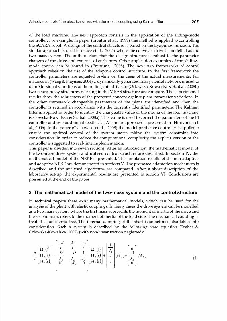
Adaptive control of the electrical drives with the elastic coupling using Kalman filter 207
of the load machine. The next approach consists in the application of the sliding-modecontroller. For example, in paper (Erbatur et al., 1999) this method is applied to controllingthe SCARA robot. A design of the control structure is based on the Lyapunov function. Thesimilar approach is used in (Hace et al., 2005) where the conveyer drive is modelled as thetwo-mass system. The authors clam that the design structure is robust to the parameterchanges of the drive and external disturbances. Other application examples of the sliding-mode control can be found in (Erenturk, 2008). The next two frameworks of controlapproach relies on the use of the adaptive control structure. In the first framework thecontroller parameters are adjusted on-line on the basis of the actual measurements. Forinstance in (Wang & Frayman, 2004) a dynamically generated fuzzy-neural network is used todamp torsional vibrations of the rolling-mill drive. In (Orlowska-Kowalska & Szabat, 2008b)two neuro-fuzzy structures working in the MRAS structure are compare. The experimentalresults show the robustness of the proposed concept against plant parameter variations. Inthe other framework changeable parameters of the plant are identified and then thecontroller is retuned in accordance with the currently identified parameters. The Kalmanfilter is applied in order to identify the changeable value of the inertia of the load machine(Orlowska-Kowalska & Szabat, 2008a). This value is used to correct the parameters of the PIcontroller and two additional feedbacks. A similar approach is presented in (Hirovonen etal., 2006). In the paper (Cychowski et al., 2008) the model predictive controller is applied oensure the optimal control of the system states taking the system constrains intoconsideration. In order to reduce the computational complexity the explicit version of thecontroller is suggested to real-time implementation.This paper is divided into seven sections. After an introduction, the mathematical model ofthe two-mass drive system and utilised control structure are described. In section IV, themathematical model of the NEKF is presented. The simulation results of the non-adaptiveand adaptive NEKF are demonstrated in sections V. The proposed adaptation mechanism isdescribed and the analysed algorithms are compared. After a short description of thelaboratory set-up, the experimental results are presented in section VI. Conclusions arepresented at the end of the paper.
2. The mathematical model of the two-mass system and the control structure
In technical papers there exist many mathematical models, which can be used for theanalysis of the plant with elastic couplings. In many cases the drive system can be modelledas a two-mass system, where the first mass represents the moment of inertia of the drive andthe second mass refers to the moment of inertia of the load side. The mechanical coupling istreated as an inertia free. The internal damping of the shaft is sometimes also taken intoconsideration. Such a system is described by the following state equation (Szabat &Orlowska-Kowalska, 2007) (with non-linear friction neglected):
( )( )( )
( )( )( )
[ ] [ ] Le
scc
s
M J
M
J
t M
t
t
K K
J J
D
J
D
J J
D
J
D
t M
t
t
dt
d
0
10
0
0
1
0
1
1
2
1
2
1
222
111
2
1
⎥⎥⎥⎥
⎦
⎤
⎢⎢⎢⎢
⎣
⎡−
+
⎥⎥⎥⎥⎥
⎦
⎤
⎢⎢⎢⎢⎢
⎣
⎡
+⎥⎥⎥
⎦
⎤
⎢⎢⎢
⎣
⎡Ω
Ω
⎥⎥⎥⎥⎥⎥
⎦
⎤
⎢⎢⎢⎢⎢⎢
⎣
⎡
−
−
−−
=⎥⎥⎥
⎦
⎤
⎢⎢⎢
⎣
⎡Ω
Ω
(1)
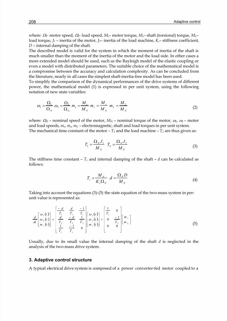
Adaptive control208
where: Ω 1- motor speed, Ω 2- load speed, M e– motor torque, M s– shaft (torsional) torque, M L–load torque, J 1 – inertia of the motor, J 2– inertia of the load machine, K c– stiffness coefficient,D – internal damping of the shaft.The described model is valid for the system in which the moment of inertia of the shaft ismuch smaller than the moment of the inertia of the motor and the load side. In other cases amore extended model should be used, such as the Rayleigh model of the elastic coupling oreven a model with distributed parameters. The suitable choice of the mathematical model isa compromise between the accuracy and calculation complexity. As can be concluded fromthe literature, nearly in all cases the simplest shaft-inertia-free model has been used.To simplify the comparison of the dynamical performances of the drive systems of differentpower, the mathematical model (1) is expressed in per unit system, using the followingnotation of new state variables:
N ΩΩ
= 11ω
N ΩΩ
= 22ω
N
ee
M
M m =
N
s
s M
M m =
N
L L
M
M m =
(2)
where: Ω N – nominal speed of the motor, M N – nominal torque of the motor, ω 1, ω 2 – motorand load speeds, me, ms, mL – electromagnetic, shaft and load torques in per unit system.The mechanical time constant of the motor – T 1 and the load machine – T 2 are thus given as:
N
N
M
J T 1
1
Ω=
N
N
M
J T 2
2
Ω=
(3)
The stiffness time constant – T c and internal damping of the shaft – d can be calculated asfollows:
N c
N c
K
M T
Ω=
N
N
M
Dd
Ω=
(4)
Taking into account the equations (3)-(5) the state equation of the two-mass system in per-unit value is represented as:
( )
( )( )
( )
( )( )
⎥⎦
⎤⎢⎣
⎡
⎥⎥⎥⎥⎥⎥
⎦
⎤
⎢⎢⎢⎢⎢⎢
⎣
⎡
−+
⎥⎥⎥
⎦
⎤
⎢⎢⎢
⎣
⎡
⎥⎥⎥⎥⎥⎥⎥
⎦
⎤
⎢⎢⎢⎢⎢⎢⎢
⎣
⎡
−
−
−−
=
⎥⎥⎥
⎦
⎤
⎢⎢⎢
⎣
⎡
L
e
s
cc
s
m
m
T
T
t m
t
t
T T
T T
d
T
d
T T
d
T
d
t m
t
t
dt
d
00
10
01
011
1
1
2
1
2
1
222
111
2
1
ω
ω
ω
ω
(5)
Usually, due to its small value the internal damping of the shaft d is neglected in theanalysis of the two-mass drive system.
3. Adaptive control structure
A typical electrical drive system is composed of a power converter-fed motor coupled to a
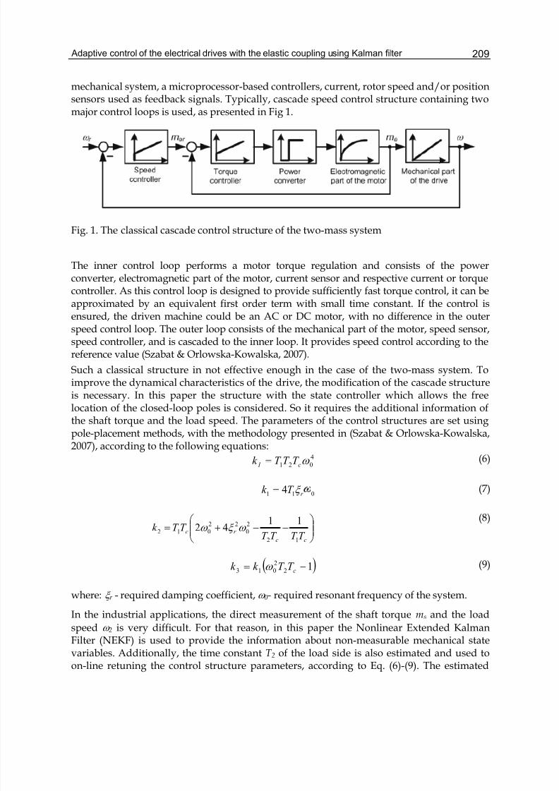
Adaptive control of the electrical drives with the elastic coupling using Kalman filter 209
mechanical system, a microprocessor-based controllers, current, rotor speed and/or positionsensors used as feedback signals. Typically, cascade speed control structure containing twomajor control loops is used, as presented in Fig 1.
Fig. 1. The classical cascade control structure of the two-mass system
The inner control loop performs a motor torque regulation and consists of the powerconverter, electromagnetic part of the motor, current sensor and respective current or torquecontroller. As this control loop is designed to provide sufficiently fast torque control, it can beapproximated by an equivalent first order term with small time constant. If the control isensured, the driven machine could be an AC or DC motor, with no difference in the outerspeed control loop. The outer loop consists of the mechanical part of the motor, speed sensor,speed controller, and is cascaded to the inner loop. It provides speed control according to thereference value (Szabat & Orlowska-Kowalska, 2007).
Such a classical structure in not effective enough in the case of the two-mass system. Toimprove the dynamical characteristics of the drive, the modification of the cascade structureis necessary. In this paper the structure with the state controller which allows the freelocation of the closed-loop poles is considered. So it requires the additional information ofthe shaft torque and the load speed. The parameters of the control structures are set usingpole-placement methods, with the methodology presented in (Szabat & Orlowska-Kowalska,2007), according to the following equations:
4
021 ω c I T T T k = (6)
011 4 ξ r T k = (7)
⎟⎟ ⎠
⎞⎜⎜⎝
⎛ −−+=
cc
r cT T T T
T T k 12
2
0
22
012
1142 ω ξ ω
(8)
( )12
2
013 −= cT T k k ω (9)
where: ξ r - required damping coefficient, ω 0- required resonant frequency of the system.
In the industrial applications, the direct measurement of the shaft torque ms and the load
speed ω 2 is very difficult. For that reason, in this paper the Nonlinear Extended KalmanFilter (NEKF) is used to provide the information about non-measurable mechanical statevariables. Additionally, the time constant T 2 of the load side is also estimated and used toon-line retuning the control structure parameters, according to Eq. (6)-(9). The estimated
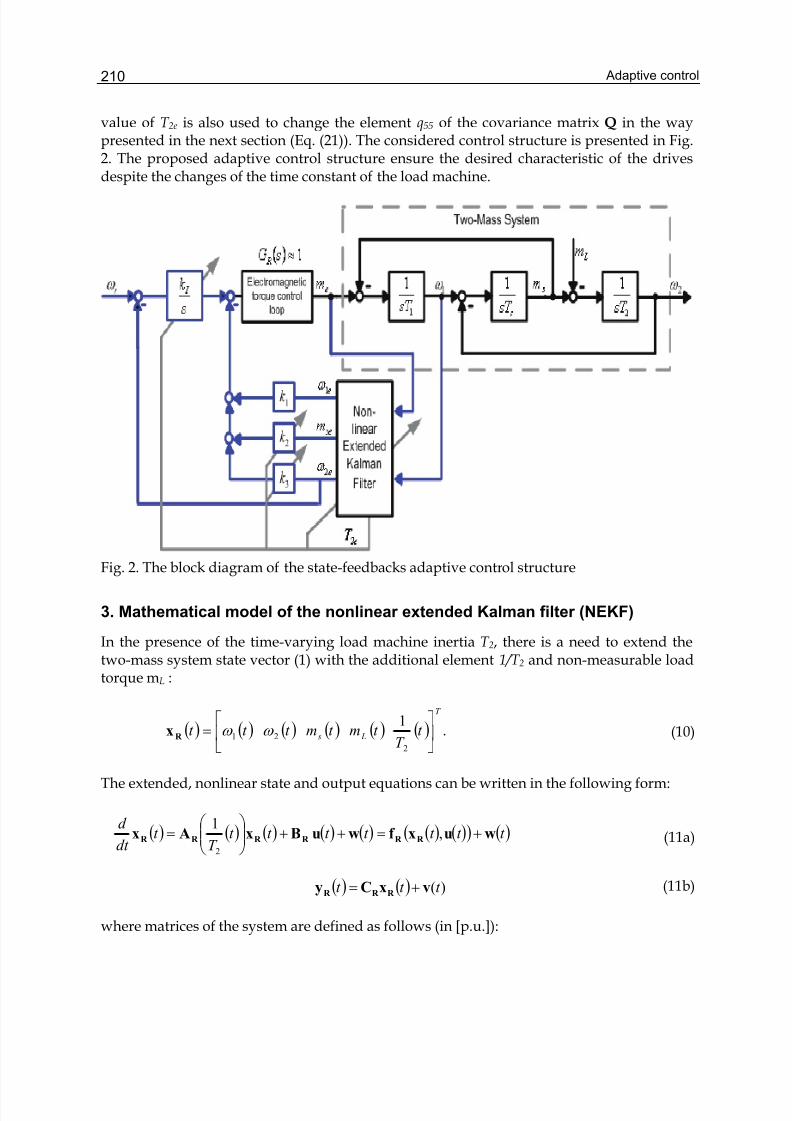
Adaptive control210
value of T 2e is also used to change the element q55 of the covariance matrix Q in the waypresented in the next section (Eq. (21)). The considered control structure is presented in Fig.2. The proposed adaptive control structure ensure the desired characteristic of the drivesdespite the changes of the time constant of the load machine.
Fig. 2. The block diagram of the state-feedbacks adaptive control structure
3. Mathematical model of the nonlinear extended Kalman filter (NEKF)
In the presence of the time-varying load machine inertia T 2, there is a need to extend thetwo-mass system state vector (1) with the additional element 1/T 2 and non-measurable loadtorque mL :
( ) ( ) ( ) ( ) ( ) ( ) .1
2
21
T
L s t T
t mt mt t t ⎥⎦
⎤⎢⎣
⎡= ω ω
R x (10)
The extended, nonlinear state and output equations can be written in the following form:
( ) ( ) ( ) ( ) ( ) ( ) ( )( ) ( )t t t t t t t T
t dt
d wuxf wuBxAx R R R R R R +=++⎟⎟
⎠
⎞⎜⎜⎝
⎛ = ,
1
2
(11a)
( ) ( ) )(t t t vxCy R R R += (11b)
where matrices of the system are defined as follows (in [p.u.]):
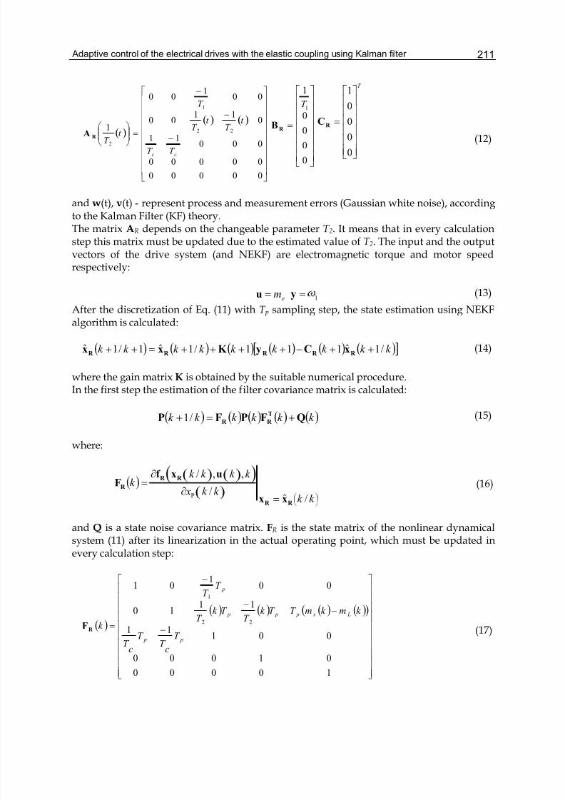
Adaptive control of the electrical drives with the elastic coupling using Kalman filter 211
( )( ) ( )
⎥⎥⎥⎥⎥⎥⎥⎥⎥
⎦
⎤
⎢⎢⎢⎢⎢⎢⎢⎢⎢
⎣
⎡
−
−
−
=⎟⎟ ⎠
⎞⎜⎜⎝
⎛
00000
00000
00011
011
00
001
00
1 22
1
2
cc T T
t T
t T
T
t T
R A
⎥⎥⎥⎥⎥⎥⎥
⎦
⎤
⎢⎢⎢⎢⎢⎢⎢
⎣
⎡
=
0
0
0
0
1
1T
R B
T
⎥⎥⎥⎥⎥⎥
⎦
⎤
⎢⎢⎢⎢⎢⎢
⎣
⎡
=
0
0
0
0
1
R C
(12)
and w(t), v(t) - represent process and measurement errors (Gaussian white noise), accordingto the Kalman Filter (KF) theory.The matrix AR depends on the changeable parameter T 2. It means that in every calculationstep this matrix must be updated due to the estimated value of T 2. The input and the outputvectors of the drive system (and NEKF) are electromagnetic torque and motor speedrespectively:
em=u 1=y (13)
After the discretization of Eq. (11) with T p sampling step, the state estimation using NEKFalgorithm is calculated:
( ) ( ) ( ) ( ) ( ) ( )[ ]k k k k k k k k k /1ˆ111/1ˆ1/1ˆ ++−++++=++ R R R R R xCyK xx (14)
where the gain matrix K is obtained by the suitable numerical procedure.In the first step the estimation of the filter covariance matrix is calculated:
( ) ( ) ( ) ( ) ( )k k k k k k QFPFPT
R R +=+ /1 (15)
where:
( )( ) ( )( )
( )k k x
k k k k
k k
k /
,,/
/ˆΡ⎟ ⎠ ⎞⎜
⎝ ⎛
∂
∂
=
=uxf
xx
FR R
R R
R
(16)
and Q is a state noise covariance matrix. FR is the state matrix of the nonlinear dynamicalsystem (11) after its linearization in the actual operating point, which must be updated inevery calculation step:
( )
( ) ( ) ( ) ( )( )
⎥⎥⎥⎥⎥⎥⎥⎥⎥⎥
⎦
⎤
⎢⎢⎢⎢⎢⎢⎢⎢⎢⎢
⎣
⎡
−
−−
−
=
10000
01000
00111
1110
001
01
22
1
p p
L s p p p
p
T
cT
T
cT
k mk mT T k T
T k T
T T
k R F
(17)
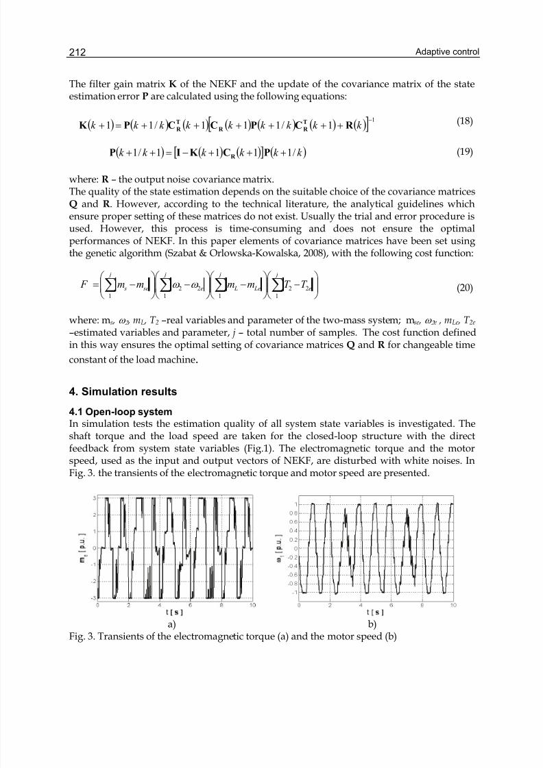
Adaptive control212
The filter gain matrix K of the NEKF and the update of the covariance matrix of the stateestimation error P are calculated using the following equations:
( ) ( ) ( ) ( ) ( ) ( ) ( )[ ] 11/111/11
−++++++=+ k k k k k k k k k R CPCCPK T
R R
T
R (18)
( ) ( ) ( )[ ] ( )k k k k k k /1111/1 +++−=++ PCK IP R (19)
where: R – the output noise covariance matrix.The quality of the state estimation depends on the suitable choice of the covariance matricesQ and R. However, according to the technical literature, the analytical guidelines whichensure proper setting of these matrices do not exist. Usually the trial and error procedure isused. However, this process is time-consuming and does not ensure the optimalperformances of NEKF. In this paper elements of covariance matrices have been set usingthe genetic algorithm (Szabat & Orlowska-Kowalska, 2008), with the following cost function:
⎟⎟ ⎠
⎞⎜⎜⎝
⎛ −⎟⎟
⎠
⎞⎜⎜⎝
⎛ −⎟⎟
⎠
⎞⎜⎜⎝
⎛ −⎟⎟
⎠
⎞⎜⎜⎝
⎛ −= ∑∑∑∑
j
e
j
Le L
j
e
j
se s T T mmmm F 1
22
11
22
1
ω ω (20)
where: ms , ω 2 , mL , T 2 –real variables and parameter of the two-mass system; mse , ω 2 e , mLe , T 2e –estimated variables and parameter, j – total number of samples. The cost function definedin this way ensures the optimal setting of covariance matrices Q and R for changeable time
constant of the load machine.
4. Simulation results
4.1 Open-loop systemIn simulation tests the estimation quality of all system state variables is investigated. Theshaft torque and the load speed are taken for the closed-loop structure with the directfeedback from system state variables (Fig.1). The electromagnetic torque and the motorspeed, used as the input and output vectors of NEKF, are disturbed with white noises. InFig. 3. the transients of the electromagnetic torque and motor speed are presented.
a) b)Fig. 3. Transients of the electromagnetic torque (a) and the motor speed (b)
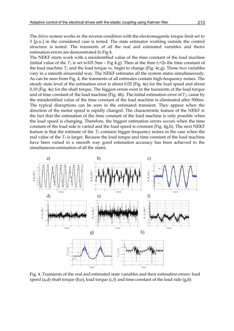
Adaptive control of the electrical drives with the elastic coupling using Kalman filter 213
The drive system works in the reverse condition with the electromagnetic torque limit set to3 [p.u.] in the considered case is tested. The state estimator working outside the controlstructure is tested. The transients of all the real and estimated variables and theirsestimation errors are demonstrated In Fig 4.The NEKF starts work with a misidentified value of the time constant of the load machine(initial value of the T 2 is set to101.5ms – Fig 4.g). Then at the time t1=2s the time constant ofthe load machine T 2 and the load torque mL begin to change (Fig. 4c,g). Those two variablesvary in a smooth sinusoidal way. The NEKF estimates all the system states simultaneously.As can be seen from Fig. 4, the transients of all estimates contain high-frequency noises. Thesteady state level of the estimation error is about 0.02 (Fig. 4e) for the load speed and about0.10 (Fig. 4e) for the shaft torque. The biggest errors exist in the transients of the load torqueand of time constant of the load machine (Fig. 4h). The initial estimation error of T 2, cause bythe misidentified value of the time constant of the load machine is eliminated after 500ms.The typical disruptions can be seen in the estimated transient. They appear when thedirection of the motor speed is rapidly changed. The characteristic feature of the NEKF isthe fact that the estimation of the time constant of the load machine is only possible whenthe load speed is changing. Therefore, the biggest estimation errors occurs when the timeconstant of the load side is varied and the load speed is constant (Fig. 4g,h). The next NEKFfeature is that the estimate of the T 2 contains bigger frequency noises in the case when thereal value of the T 2 is larger. Because the load torque and time constant of the load machinehave been varied in a smooth way good estimation accuracy has been achieved in thesimultaneous estimation of all the states.
a) b) c)
d) e) f)
g) h)
Fig. 4. Transients of the real and estimated state variables and their estimation errors: loadspeed (a,d) shaft torque (b,e), load torque (c,f) and time constant of the load side (g,h)
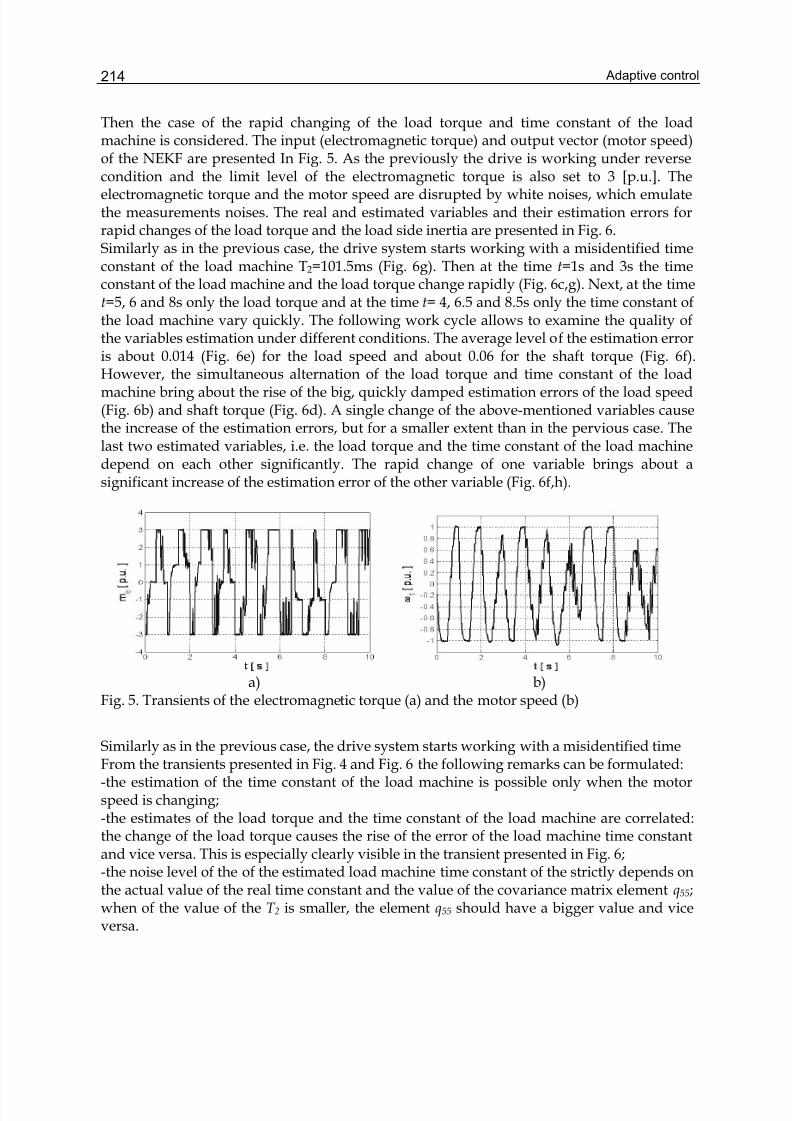
Adaptive control214
Then the case of the rapid changing of the load torque and time constant of the loadmachine is considered. The input (electromagnetic torque) and output vector (motor speed)of the NEKF are presented In Fig. 5. As the previously the drive is working under reversecondition and the limit level of the electromagnetic torque is also set to 3 [p.u.]. Theelectromagnetic torque and the motor speed are disrupted by white noises, which emulatethe measurements noises. The real and estimated variables and their estimation errors forrapid changes of the load torque and the load side inertia are presented in Fig. 6.Similarly as in the previous case, the drive system starts working with a misidentified timeconstant of the load machine T2=101.5ms (Fig. 6g). Then at the time t=1s and 3s the timeconstant of the load machine and the load torque change rapidly (Fig. 6c,g). Next, at the timet=5, 6 and 8s only the load torque and at the time t= 4, 6.5 and 8.5s only the time constant ofthe load machine vary quickly. The following work cycle allows to examine the quality ofthe variables estimation under different conditions. The average level of the estimation erroris about 0.014 (Fig. 6e) for the load speed and about 0.06 for the shaft torque (Fig. 6f).However, the simultaneous alternation of the load torque and time constant of the loadmachine bring about the rise of the big, quickly damped estimation errors of the load speed(Fig. 6b) and shaft torque (Fig. 6d). A single change of the above-mentioned variables causethe increase of the estimation errors, but for a smaller extent than in the pervious case. Thelast two estimated variables, i.e. the load torque and the time constant of the load machinedepend on each other significantly. The rapid change of one variable brings about asignificant increase of the estimation error of the other variable (Fig. 6f,h).
a) b)Fig. 5. Transients of the electromagnetic torque (a) and the motor speed (b)
Similarly as in the previous case, the drive system starts working with a misidentified timeFrom the transients presented in Fig. 4 and Fig. 6 the following remarks can be formulated:-the estimation of the time constant of the load machine is possible only when the motorspeed is changing;-the estimates of the load torque and the time constant of the load machine are correlated:the change of the load torque causes the rise of the error of the load machine time constantand vice versa. This is especially clearly visible in the transient presented in Fig. 6;-the noise level of the of the estimated load machine time constant of the strictly depends onthe actual value of the real time constant and the value of the covariance matrix element q55;when of the value of the T 2 is smaller, the element q55 should have a bigger value and viceversa.
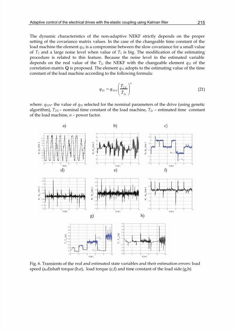
Adaptive control of the electrical drives with the elastic coupling using Kalman filter 215
The dynamic characteristics of the non-adaptive NEKF strictly depends on the propersetting of the covariance matrix values. In the case of the changeable time constant of theload machine the element q55 is a compromise between the slow covariance for a small valueof T 2 and a large noise level when value of T 2 is big. The modification of the estimatingprocedure is related to this feature. Because the noise level in the estimated variabledepends on the real value of the T 2, the NEKF with the changeable element q55 of thecorrelation matrix Q is proposed. The element q55 adopts to the estimating value of the timeconstant of the load machine according to the following formula:
n
e
N
N T
T qq ⎟⎟
⎠
⎞⎜⎜⎝
⎛ =
2
2
5555 (21)
where: q55N - the value of q55 selected for the nominal parameters of the drive (using geneticalgorithm), T 2N – nominal time constant of the load machine, T 2e – estimated time constantof the load machine, n – power factor.
a) b) c)
d) e) f)
g) h)
Fig. 6. Transients of the real and estimated state variables and their estimation errors: loadspeed (a,d)shaft torque (b,e), load torque (c,f) and time constant of the load side (g,h)
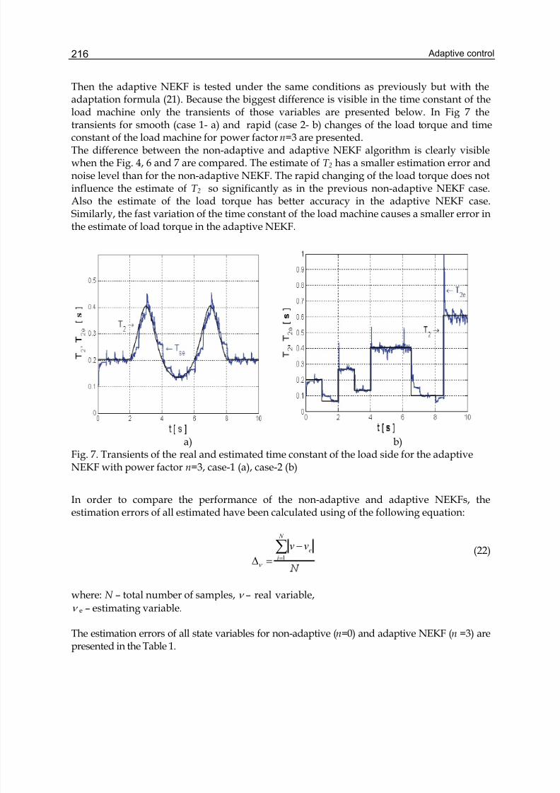
Adaptive control216
Then the adaptive NEKF is tested under the same conditions as previously but with theadaptation formula (21). Because the biggest difference is visible in the time constant of theload machine only the transients of those variables are presented below. In Fig 7 thetransients for smooth (case 1- a) and rapid (case 2- b) changes of the load torque and timeconstant of the load machine for power factor n=3 are presented.The difference between the non-adaptive and adaptive NEKF algorithm is clearly visiblewhen the Fig. 4, 6 and 7 are compared. The estimate of T 2 has a smaller estimation error andnoise level than for the non-adaptive NEKF. The rapid changing of the load torque does notinfluence the estimate of T 2 so significantly as in the previous non-adaptive NEKF case.Also the estimate of the load torque has better accuracy in the adaptive NEKF case.Similarly, the fast variation of the time constant of the load machine causes a smaller error inthe estimate of load torque in the adaptive NEKF.
a) b)Fig. 7. Transients of the real and estimated time constant of the load side for the adaptiveNEKF with power factor n=3, case-1 (a), case-2 (b)
In order to compare the performance of the non-adaptive and adaptive NEKFs, theestimation errors of all estimated have been calculated using of the following equation:
vv N
i
e∑=
−=Δ 1
ν
(22)
where: N – total number of samples, ν – real variable,
ν e – estimating variable.
The estimation errors of all state variables for non-adaptive (n=0) and adaptive NEKF (n =3) arepresented in the Table 1.
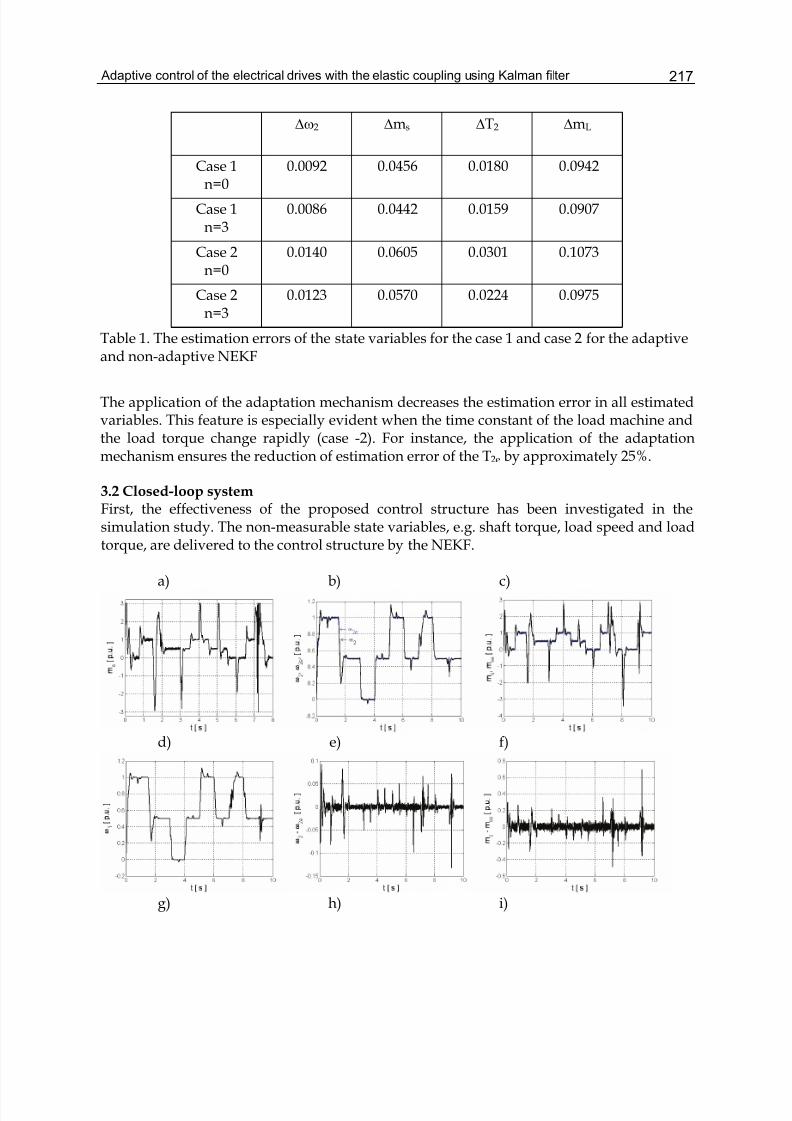
Adaptive control of the electrical drives with the elastic coupling using Kalman filter 217
Δω2 Δms ΔT2 ΔmL
Case 1n=0
0.0092 0.0456 0.0180 0.0942
Case 1n=3
0.0086 0.0442 0.0159 0.0907
Case 2n=0
0.0140 0.0605 0.0301 0.1073
Case 2n=3
0.0123 0.0570 0.0224 0.0975
Table 1. The estimation errors of the state variables for the case 1 and case 2 for the adaptiveand non-adaptive NEKF
The application of the adaptation mechanism decreases the estimation error in all estimatedvariables. This feature is especially evident when the time constant of the load machine andthe load torque change rapidly (case -2). For instance, the application of the adaptationmechanism ensures the reduction of estimation error of the T2e by approximately 25%.
3.2 Closed-loop systemFirst, the effectiveness of the proposed control structure has been investigated in thesimulation study. The non-measurable state variables, e.g. shaft torque, load speed and loadtorque, are delivered to the control structure by the NEKF.
a) b) c)
d) e) f)
g) h) i)
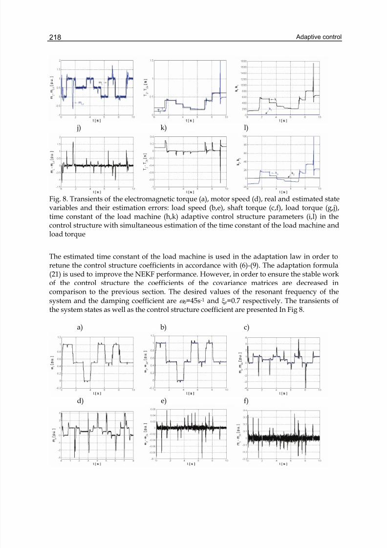
Adaptive control218
j) k) l)
Fig. 8. Transients of the electromagnetic torque (a), motor speed (d), real and estimated statevariables and their estimation errors: load speed (b,e), shaft torque (c,f), load torque (g,j),time constant of the load machine (h,k) adaptive control structure parameters (i,l) in thecontrol structure with simultaneous estimation of the time constant of the load machine andload torque
The estimated time constant of the load machine is used in the adaptation law in order toretune the control structure coefficients in accordance with (6)-(9). The adaptation formula(21) is used to improve the NEKF performance. However, in order to ensure the stable workof the control structure the coefficients of the covariance matrices are decreased incomparison to the previous section. The desired values of the resonant frequency of the
system and the damping coefficient are ω 0=45s-1 and ξr=0.7 respectively. The transients ofthe system states as well as the control structure coefficient are presented In Fig 8.
a) b) c)
d) e) f)
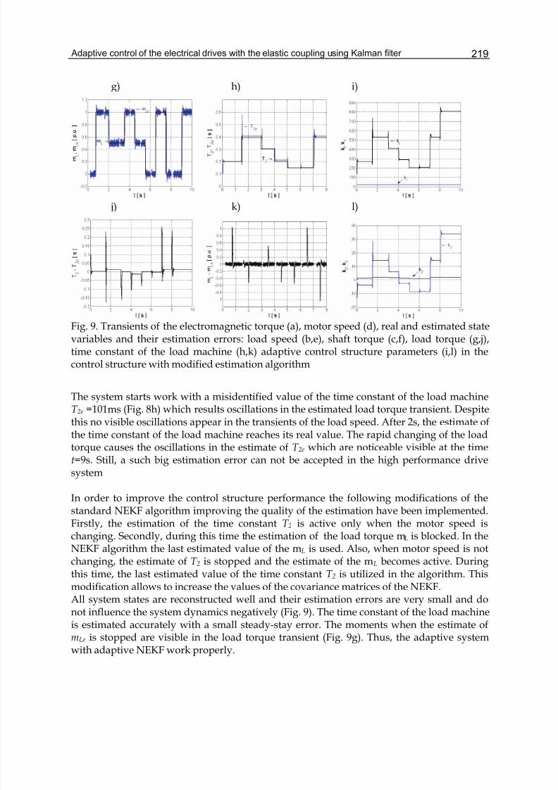
Adaptive control of the electrical drives with the elastic coupling using Kalman filter 219
g) h) i)
j) k) l)
Fig. 9. Transients of the electromagnetic torque (a), motor speed (d), real and estimated statevariables and their estimation errors: load speed (b,e), shaft torque (c,f), load torque (g,j),time constant of the load machine (h,k) adaptive control structure parameters (i,l) in thecontrol structure with modified estimation algorithm
The system starts work with a misidentified value of the time constant of the load machineT 2e =101ms (Fig. 8h) which results oscillations in the estimated load torque transient. Despitethis no visible oscillations appear in the transients of the load speed. After 2s, the estimate ofthe time constant of the load machine reaches its real value. The rapid changing of the loadtorque causes the oscillations in the estimate of T 2e which are noticeable visible at the timet=9s. Still, a such big estimation error can not be accepted in the high performance drivesystem
In order to improve the control structure performance the following modifications of thestandard NEKF algorithm improving the quality of the estimation have been implemented.Firstly, the estimation of the time constant T 2 is active only when the motor speed ischanging. Secondly, during this time the estimation of the load torque mL is blocked. In theNEKF algorithm the last estimated value of the mL is used. Also, when motor speed is notchanging, the estimate of T 2 is stopped and the estimate of the mL becomes active. Duringthis time, the last estimated value of the time constant T 2 is utilized in the algorithm. Thismodification allows to increase the values of the covariance matrices of the NEKF.All system states are reconstructed well and their estimation errors are very small and donot influence the system dynamics negatively (Fig. 9). The time constant of the load machineis estimated accurately with a small steady-stay error. The moments when the estimate ofmLe is stopped are visible in the load torque transient (Fig. 9g). Thus, the adaptive systemwith adaptive NEKF work properly.
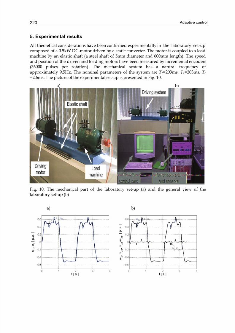
Adaptive control220
5. Experimental results
All theoretical considerations have been confirmed experimentally in the laboratory set-up
composed of a 0.5kW DC-motor driven by a static converter. The motor is coupled to a loadmachine by an elastic shaft (a steel shaft of 5mm diameter and 600mm length). The speedand position of the driven and loading motors have been measured by incremental encoders(36000 pulses per rotation). The mechanical system has a natural frequency ofapproximately 9.5Hz. The nominal parameters of the system are T 1=203ms, T 2=203ms, T c=2.6ms. The picture of the experimental set-up is presented in Fig. 10.
a) b)
Fig. 10. The mechanical part of the laboratory set-up (a) and the general view of thelaboratory set-up (b)
a) b)
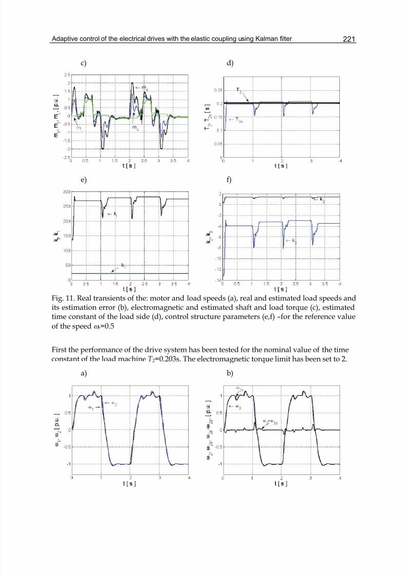
Adaptive control of the electrical drives with the elastic coupling using Kalman filter 221
c) d)
e) f)
Fig. 11. Real transients of the: motor and load speeds (a), real and estimated load speeds andits estimation error (b), electromagnetic and estimated shaft and load torque (c), estimatedtime constant of the load side (d), control structure parameters (e,f) –for the reference value
of the speed ω r =0.5
First the performance of the drive system has been tested for the nominal value of the timeconstant of the load machine T 2=0.203s. The electromagnetic torque limit has been set to 2.
a) b)
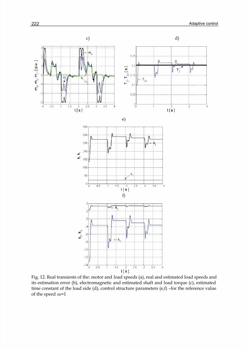
Adaptive control222
c) d)
e)
f)
Fig. 12. Real transients of the: motor and load speeds (a), real and estimated load speeds andits estimation error (b), electromagnetic and estimated shaft and load torque (c), estimatedtime constant of the load side (d), control structure parameters (e,f) –for the reference value
of the speed ω r =1
Adaptive control of the electrical drives with the elastic coupling using Kalman filter 223
The system works with the reference value of the speed set to 0.5. According to theadaptation procedure described in the previous section during start-up the estimate of themLe is blocked and the estimate of the T 2e is activated which is observable in Fig. 11c,d. Whenthe control error decreases below 0.05, the estimate T 2e is blocked and the mLe. At the timet1=0.4s the nominal load torque is applied to the system. This affects the system speed in anegative way and some disruption is visible in its transients. The load torque is switched offat the time t2=0.8s and the non-zero value of the estimate of the mLe comes from the frictiontorques. At the time t3=1s the system begins to reverse. When the value of the system speedis negative, no external torque is applied to the system. The drive reverses again at the timet4=2s and then the work cycle is repeated. Clearly, the adaptive control structure with theNEKF works properly. The load speed as well as the time constant of the load machine areestimated with small errors. The transients of the control structure parameters are presentedin Fig. 11 e,f. They vary (except k1) with the estimated value of the T 2e.Next the control structure with the electromagnetic torque limit set to 3 has been examined.The work cycle is identical as previously. But the reference speed is set to the nominal value.The transients of the system are presented in Fig. 12.Similarly as before, the initial value of the time constant of the load machine is set toT 2e=0.1015s. After the start-up it reaches its real value almost without an error. During thenext reversal the estimate of the T 2 oscillates around the real value. However, it should bepointed out that the estimation error does not exceed a few percent of the real value. Theestimate of the T 2 is reconstructed very well. Small errors appear in its transient during thetime when the load torque is switched on and off and during the reversal. The adaptivecontrol structure with the state controller works in a stable way.
6. Conclusion
In order to damp the torsional vibrations, which could destroy the mechanical couplingbetween the driven and loading machine, the control structure with state controller isapplied. The control structure coefficients depend on the time constant of the load sidemachine. In the case of the system with changeable load side inertia, there is a need toestimate this parameter and adapt the control structure gains in accordance with the actualestimated value. The application of the adaptive control structure ensures the requiredtransient of the load speed despite the changeable load side inertia. In order to use theadaptive control structure, there is a need to choose a state estimator, which has to estimatethe non-measurable system state variables and changeable parameters of the system. In thispaper, the non-adaptive and adaptive nonlinear extended Kalman filter (NEKF) is tested.Parameters of the covariance matrices Q and R are selected using the genetic algorithm withspecial cost function. The application of the global optimization technique allows to reachthe global solution according to the defined cost function. However, the application of thegenetic algorithm is possible only as an off-line process due to a long calculation time. Toensure the optimal values of the covariance matrix Q, despite the load side parameterchanges, the adaptation mechanism is developed. The suitable on-line change of thecovariance matrix element q55 is proposed, according to the estimated value of the load sidetime constant. It is proved by simulation and experimental tests that the proposed controlstructure is effective for damping the torsional oscillation of two-mass drive system, also in
Adaptive control224
the case of wide range changes of load side inertia.
7. References
Beineke, S., Schütte, F. & Grotstollen H. (1997). Comparison of Methods for State Estimationand On-Line Identification in Speed and Position Control Loops , Proc. of the Intern.Conf. European Power Electronics EPE’97 , pp. 3.364-3.369, Norway.
Cychowski M. T., Delaney K. and Szabat K. (2008), Explicit Model Predictive Control of theDrive System with Elastic Coupling, Proc. of 13th International Conference on Power Electronics and Motion Control EPE-PEMC 2008, on. cd, Poland
Erbatur, K., Kaynak, O. & Sabanovic A. (1999). A Study on Robustness Property of SlidingMode Controllers: A Novel Design and Experimental Investigations, IEEETransaction on Industrial Electronics, Vol. 46, No. 5 , pp. 1012-1018.
Erenturk, K. (2008). Nonlinear two-mass system control with sliding-mode and optimisedproportional and integral derivative controller combined with a grey estimator,Control Theory & Applications, IET , Vol. 2, No. 7, pp. 635 – 642.
Ellis, G. & Lorenz, R.D. (2000), Resonant load control methods for industrial servo drives.Proc. of the IEEE Industry Application Society Annual Meeting, pp. 1438-1445.
Ferretti, G., Magnoni, G. A. & Rocco, P. (2004). Impedance Control for Elastic Joint IndustrialManipulators, IEEE Trans. on Robotics and Automation, Vol. 20, pp. 488-498.
Ferretti, G., Magnoni, G. A., Rocco, P., Vigano, L. & Rusconi, A. (2005). On the Use of TorqueSensors in a Space Robotics Application, : Proc. on the IEEE/RSJ InternationalConference on Intelligent Robots and Systems IROS 2005, pp. 1947- 1952, Canada.
Gawronski, W., Racho, C. S. & Mellstrom, J. A. (1995). Application of the LQG andFeedforward Controllers to the Deep Space Network Antennas, IEEE Trans. onControl System Technology, Vol. 3, No. 4, pp. 417-421.
Gu D. W., Petkov P. H., Konstantinov M. M. (2005). Robust Control Design with Matlab®,Springer .
Hace. A., Jezernik, K. & Sabanovic, A. (2005). Improved Design of VSS Controller for aLinear Belt-Driven Servomechanism, IEEE/ASME Trans. on Mechatronic, Vol. 10, No.4, pp. 385-390.
Hirovonen, M., Pyrhonen, O. & Handroos H. (2006). Adaptive nonlinear velocity controllerfor a flexible mechanism of a linear motor, Mechatronic, Elsevier, Vol. 16, No. 5, pp.279-290.
Hori, Y., Sawada, H. & Chun, Y. (1999). Slow resonance ratio control for vibration suppressionand disturbance rejection in torsional system, IEEE Trans. on Industrial Electronics, Vol.46, No. 1, pp. 162-168.
Horwitz, R., Li, Y., Oldham, K., Kon, S. & Huang, X. (2007), Dual-stage servo systems andvibration compensation in computer hard disk drives, Control Engineering Practice,Vol. 15, pp. 291-305.
Huang, A.,C. & Chen, Y., C. (2004). Adaptive Sliding Control for Single-Ling Flexible-JointRobot With Mismatched Uncertainties, IEEE Trans. on Control System Technology, Vol. 12, pp. 770-775.
Itoh D., Iwasaki M., Matsui N. (2004). Optimal Design of Robust Vibration SuppressionController Using Genetic Algorithms, IEEE Transaction on Industrial Electronics, Vol.51, No. 5, pp. 947-953.
Adaptive control of the electrical drives with the elastic coupling using Kalman filter 225
Ji, J. K. & Sul, S. K. (1995). Kalman Filter and LQ Based Speed Controller for TorsionalVibration Suppression in a 2-Mass Motor Drive System, IEEE Trans. on IndustrialElectronics, Vol. 42, No. 6, pp. 564-571.
Katsura, S. & Ohnishi, K. (2005). Force Servoing by Flexible Manipulator Based onResonance Ratio Control, Proc. of the IEEE International Symposium on IndustrialElectronics ISIE 2005, pp. 1343-1348, Croatia.
Michels, K., Klawonn, F., Kruse, R. & Nürnberger, A. (2006). Fuzzy Control – Fundamentals,Stability and Design of Fuzzy Controllers, Springer .
Ohno, K. & Hara, T. (2006). Adaptive Resonant Mode Compensation for hard Dick Drives, ,IEEE Trans. on Industrial Electronics, Vol. 53, No. 2, pp. 624-629.
Orlowska-Kowalska, T. & Szabat, K. (2008). Damping of Torsional Vibrations in Two-MassSystem Using Adaptive Sliding Neuro-Fuzzy Approach, IEEE Transactions onIndustrial Informatics, Vol. 4, No. 1, pp. 47-57.
O’Sullivan, T., Bingham, C. C. & Schofield, N. (2007), Enhanced Servo-Control Performanceof Dual-Mass System, IEEE Trans. on Ind. Electronics, Vol. 54, No. 3, pp. 1387-1398.
Qiao, R., Zhu, Q. M., Li, S. Y. & Winfield, A. (2002). Torsional Vibration Suppression of a 2-Mass Main Drive System of Rolling Mill with KF Enhanced Pole Placement, Proc. of the 4th World Congress on Intelligent Control and Automation, pp. 206-210, China.
Shen, B. H. & Tsai, M. C. (2006) Robust dynamic stiffness design of linear servomotor drives,Control Engineering Practice, Vol. 14, pp. 1325-1336.
Sugiura, K. & Hori, Y. (1996). Vibration Suppression in 2- and 3-Mass System Based on theFeedback of Imperfect Derivative of the Estimated Torsional Torque, IEEE Trans. onIndustrial Electronics, Vol. 43, No. 2, pp. 56-64.
Suh, G., Hyun, D. S., Park, J. I., Lee, K. D. & Lee, S. G. (2001), Design of a Pole PlacementController for Reducing Oscillation and Settling Time in a Two-Inertia System,Proc. of 24th Annual Conference of the IEEE Industrial Electronics Society IECON’01,pp.1439-1444, USA.
Szabat, K. & Orłowska-Kowalska, T. (2007). Vibration Suppression in Two-Mass DriveSystem using PI Speed Controller and Additional Feedbacks – Comparative Study,IEEE Trans. on Industrial Electronics, Vol. 54, No. 2, pp.1193-1206.
Szabat, K. & Orlowska-Kowalska, T. (2008). Performance Improvement of Industrial DrivesWith Mechanical Elasticity Using Nonlinear Adaptive Kalman Filter, IEEETransactions on Industrial Electronics, Vol. 55, No. 3, pp. 1075-1084.
Valenzuela, M. A., Bentley, J. M. & Lorenz, R. D. (2005). Evaluation of Torsional Oscillationsin Paper Machine Sections, IEEE Trans. on Industrial Applications, Vol. 41, No. 2, pp.493-501.
Vukosovic, S., N. & Stojic, M. R., (1998). Suppression of Torsional Oscillations in a High-Performance Speed Servo Drive, IEEE Trans. on Industrial Electronic, Vol. 45, No. 1,pp. 108-117.
Wertz H., Beineke S., Frőhleke N., Bolognani S., Unterkofler K., Zigliotto M. & Zordan M.(1999) Computer Aided Commissioning of Speed and Position Control forElectrical Drives with Identification of Mechanical Load, Proc. of the Thirty-FourthIAS Annual Meeting Industry Applications Conference, pp. 4.1372-4.2379, USA.
Wang L., Frayman Y. (2002). A Dynamically Generated Fuzzy Neural Network and itsApplication to Torsional Vibration Control of Tandem Cold Rolling Mill Spindles,Engineering Applications of Artificial Intelligence, Vol.15, No. 6, pp. 541-550.

Adaptive control226
Zhang, G. & Furusho, J. (2000). Speed Control of Two-Inertia System by PI/PID Control, IEEE Trans. on Industrial Electronics, Vol. 47, No. 3, pp. 603-609.
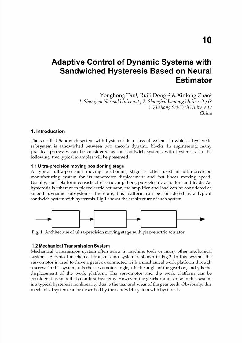
10
Adaptive Control of Dynamic Systems withSandwiched Hysteresis Based on Neural
Estimator
Yonghong Tan1, Ruili Dong1,2 & Xinlong Zhao3
1. Shanghai Normal University 2. Shanghai Jiaotong University &3. Zhejiang Sci-Tech University
China
1. Introduction
The so-called Sandwich system with hysteresis is a class of systems in which a hystereticsubsystem is sandwiched between two smooth dynamic blocks. In engineering, manypractical processes can be considered as the sandwich systems with hysteresis. In thefollowing, two typical examples will be presented.
1.1 Ultra-precision moving positioning stageA typical ultra-precision moving positioning stage is often used in ultra-precisionmanufacturing system for its nanometer displacement and fast linear moving speed.Usually, such platform consists of electric amplifiers, piezoelectric actuators and loads. Ashysteresis is inherent in piezoelectric actuator, the amplifier and load can be considered assmooth dynamic subsystems. Therefore, this platform can be considered as a typicalsandwich system with hysteresis. Fig.1 shows the architecture of such system.
Fig. 1. Architecture of ultra-precision moving stage with piezoelectric actuator
1.2 Mechanical Transmission SystemMechanical transmission system often exists in machine tools or many other mechanicalsystems. A typical mechanical transmission system is shown in Fig.2. In this system, theservomotor is used to drive a gearbox connected with a mechanical work platform througha screw. In this system, u is the servomotor angle, x is the angle of the gearbox, and y is thedisplacement of the work platform. The servomotor and the work platform can beconsidered as smooth dynamic subsystems. However, the gearbox and screw in this systemis a typical hysteresis nonlinearity due to the tear and wear of the gear teeth. Obviously, thismechanical system can be described by the sandwich system with hysteresis.
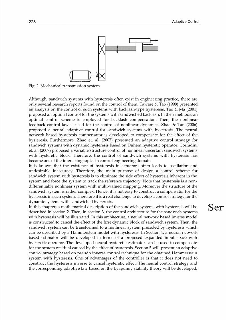
Adaptive Control228
Fig. 2. Mechanical transmission system
Although, sandwich systems with hysteresis often exist in engineering practice, there areonly several research reports found on the control of them. Taware & Tao (1999) presentedan analysis on the control of such systems with backlash-type hysteresis. Tao & Ma (2001)proposed an optimal control for the systems with sandwiched backlash. In their methods, anoptimal control scheme is employed for backlash compensation. Then, the nonlinearfeedback control law is used for the control of nonlinear dynamics. Zhao & Tan (2006)proposed a neural adaptive control for sandwich systems with hysteresis. The neuralnetwork based hysteresis compensator is developed to compensate for the effect of thehysteresis. Furthermore, Zhao et. al. (2007) presented an adaptive control strategy forsandwich systems with dynamic hysteresis based on Duhem hysteretic operator. Corradiniet. al. (2007) proposed a variable structure control of nonlinear uncertain sandwich systemswith hysteretic block. Therefore, the control of sandwich systems with hysteresis hasbecome one of the interesting topics in control engineering domain.It is known that the existence of hysteresis in actuators often leads to oscillation andundesirable inaccuracy. Therefore, the main purpose of design a control scheme forsandwich system with hysteresis is to eliminate the side effect of hysteresis inherent in thesystem and force the system to track the reference trajectory. Note that hysteresis is a non-differentiable nonlinear system with multi-valued mapping. Moreover the structure of thesandwich system is rather complex. Hence, it is not easy to construct a compensator for thehysteresis in such system. Therefore it is a real challenge to develop a control strategy for thedynamic systems with sandwiched hysteresis.In this chapter, a mathematical description of the sandwich systems with hysteresis will bedescribed in section 2. Then, in section 3, the control architecture for the sandwich systemswith hysteresis will be illustrated. In this architecture, a neural network based inverse modelis constructed to cancel the effect of the first dynamic block of sandwich system. Then, thesandwich system can be transformed to a nonlinear system preceded by hysteresis whichcan be described by a Hammerstein model with hysteresis. In Section 4, a neural networkbased estimator will be developed in terms of a proposed expanded input space withhysteretic operator. The developed neural hysteretic estimator can be used to compensatefor the system residual caused by the effect of hysteresis. Section 5 will present an adaptivecontrol strategy based on pseudo inverse control technique for the obtained Hammersteinsystem with hysteresis. One of advantages of the controller is that it does not need toconstruct the hysteresis inverse to cancel hysteretic effect. The neural control strategy andthe corresponding adaptive law based on the Lyapunov stability theory will be developed.
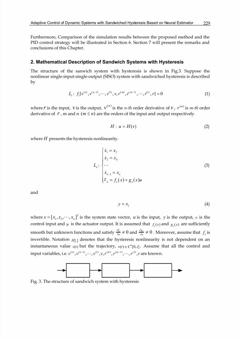
Adaptive Control of Dynamic Systems with Sandwiched Hysteresis Based on Neural Estimator 229
Furthermore, Comparison of the simulation results between the proposed method and thePID control strategy will be illustrated in Section 6. Section 7 will present the remarks andconclusions of this Chapter.
2. Mathematical Description of Sandwich Systems with Hysteresis
The structure of the sanwich system with hysteresis is shown in Fig.3. Suppose thenonlinear single-input-single-output (SISO) system with sandwiched hysteresis is describedby
i L : ( ) ( 1) (1) ( ) ( 1) (1)[ , , , , , , , , , ] 0n n m m
i f v v v v r r r r − − =L L (1)
where r is the input, v is the output,( )nv is the n-th order derivative of v , ( )mr is m-th order
derivative of r , m and n ( )m n≤ are the orders of the input and output respectively.
H : ( )u H v= (2)
where H presents the hysteresis nonlinearity.
o L :
1 2
2 3
1
( ) ( )
n n
n o o
x x
x x
x x
f x g x u
−
=⎧⎪ =⎪⎪⎨⎪ =⎪
= +⎪⎩
&
&
L
&
&
(3)
and
1 y x= (4)
where 1 2[ , , , ]T
n x x x x= L is the system state vector, u is the input, y is the output, v is the
control input and u is the actuator output. It is assumed that ( )o f x and ( )o g x are sufficiently
smooth but unknown functions and satisfy 0o f
u
∂
∂≠ and 0o g
u
∂
∂≠ . Moreover, assume that
o f is
invertible. Notation [.] H denotes that the hysteresis nonlinearity is not dependent on an
instantaneous value ( )v t but the trajectory, 0( ) [0, ]v t C t ∈ . Assume that all the control and
input variables, i.e. ( ) ( 1) (1) ( ) ( 1) (1), , , , , , , , ,n n m mv v v v r r r r − −L L are known.
Fig. 3. The structure of sandwich system with hysteresis
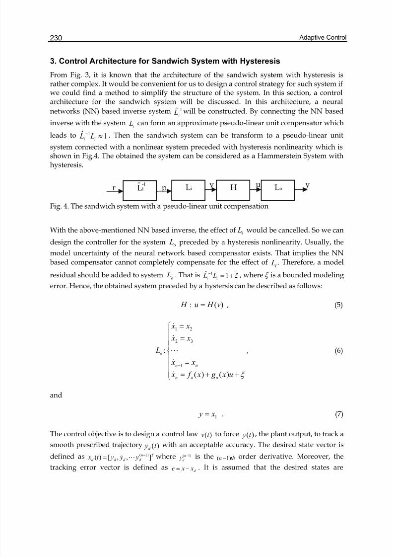
Adaptive Control230
3. Control Architecture for Sandwich System with Hysteresis
From Fig. 3, it is known that the architecture of the sandwich system with hysteresis israther complex. It would be convenient for us to design a control strategy for such system ifwe could find a method to simplify the structure of the system. In this section, a controlarchitecture for the sandwich system will be discussed. In this architecture, a neural
networks (NN) based inverse system 1ˆi L− will be constructed. By connecting the NN based
inverse with the systemi
L can form an approximate pseudo-linear unit compensator which
leads to 1ˆ 1i i L L− ≈ . Then the sandwich system can be transform to a pseudo-linear unit
system connected with a nonlinear system preceded with hysteresis nonlinearity which isshown in Fig.4. The obtained the system can be considered as a Hammerstein System withhysteresis.
Fig. 4. The sandwich system with a pseudo-linear unit compensation
With the above-mentioned NN based inverse, the effect of i L would be cancelled. So we can
design the controller for the system o L preceded by a hysteresis nonlinearity. Usually, the
model uncertainty of the neural network based compensator exists. That implies the NN
based compensator cannot completely compensate for the effect ofi L . Therefore, a model
residual should be added to system o L . That is 1ˆ 1i i L L− = +ξ , whereξ is a bounded modeling
error. Hence, the obtained system preceded by a hystersis can be described as follows:
H : ( )u H v= , (5)
o L :
1 2
2 3
1
( ) ( )
n n
n o o
x x
x x
x x
x f x g x u ξ
−
=⎧⎪ =⎪⎪⎨⎪ =⎪
= + +⎪⎩
&
&
L
&
&
, (6)
and
1 y x= . (7)
The control objective is to design a control law ( )v t to force ( ) y t , the plant output, to track a
smooth prescribed trajectory ( )d y t with an acceptable accuracy. The desired state vector is
defined as ( 1)( ) [ , , ]n T
d d d d x t y y y−= & L where ( 1)n
d y − is the ( 1)n th− order derivative. Moreover, the
tracking error vector is defined asd e x x= − . It is assumed that the desired states are
Li Lo Hp v u yr Li -1^
Adaptive Control of Dynamic Systems with Sandwiched Hysteresis Based on Neural Estimator 231
bounded, i.e.d d x X ≤ . Moreover, ξ denotes bounded disturbance caused by NN based
inverse, where ξ ξ ≤ , and 0 N ξ > .
Define the filtered tracking error as
1 2 1[ , ,1] [ ,1]T
ne eτ λ λ λ −= = ΛL (8)
where 1 2 1[ , ]T
nλ λ λ −Λ = L is a parameter vector to be designed. Suppose
1 2
1 1
n n
n s s− −−+ + +Lλ λ
is Hurwitz. Differentiating (8) and using (6), it results in
[0, ] ( ) ( ) [0, ]n T n T
n d o o d x y e f x g x u y e= − + Λ = + − + Λ +& &τ ξ (9)
As u is the output of hysteresis which is usually unknown, an invertible function ˆ ( , ) f x v is
introduced to approximate ( ) ( )o o f x g x u+ . Adding and subtracting ˆ ( , ) f x v to and from the
right hand side of (9), it yields
( )
( )
( )
ˆ( ) ( ) ( , ) [0, ]
ˆ( , ) ( , ) [0, ]
( , , ) [0, ]
n T
o o d
n T
d
n T
d
f x g x u f x v y e
F x u f x v y e
f x v u y e
τ δ ξ
δ ξ
δ ξ
= + + − − + Λ +
= + − − + Λ +
= + − + Λ +
&
%
(10)
where ˆ ( , ) f x vδ = is the so called pseudo-control (Calis & Hovakimyan, 2001) and
(Hovakimyan & Nandi ,2002), ( , ) ( ) ( )o o F x u f x g x u= + and ˆ( , , ) ( , ) ( , ) f x v u F x u f x v= −% is the
system residual. As ˆ ( , ) f x v is invertible with respect to v and satisfies (Calis & Hovakimyan,
2001):
1.ˆ
sgn sgn F u f
u v v
∂ ∂ ∂=
∂ ∂ ∂, (11)
and
2.ˆ 1
02
f F u
v u v
∂ ∂ ∂> >
∂ ∂ ∂. (12)
In order to design the corresponding control strategy, the approximation of the nonlinear
residual ( , , ) f x v u% is required. Neural networks would be one of the recommended
alternatives to model this residual. However, ( , , ) f x v u% involves the characteristic of
Adaptive Control232
hysteresis, the traditional nonlinear identification methods such as neural modelingtechnique usually cannot be directly applied to the modeling of it since the hysteresis is anon-linearity with multi-valued mapping (Adly & Abd-El-Hafiz, 1998). In Section 4, we will
present a method to construct the neural estimator for ( , , ) f x v u% to compensate for the effect
of hysteresis. Moreover, a corresponding adaptive control method based on the controlarchieture stated-above will be illustrated in Section 5.
4. Neural Estimator for System Residual
In order to approximate the system residual, neural network can be considered as analternative. However, the system residual contains the characteristic of hysteresis which is asystem with multi-valued mapping. In this section, a hysteretic operator is proposed toconstruct an expanded input space so as to transform the multi-valued mapping ofhysteresis into a one-to-one mapping (Zhao & Tan, 2008). Thus, the neural networks can beused for modeling of hysteresis based on the expanded input space with the hystereticoperator. The proposed hysteretic operator is defined as:
| |( ) (1 )( ) ( ) p x x
p ph x e x x h x− −
= − − + , (13)
where is the current input, ( )h x is the current output, p is the dominant extremum
adjacent to the current input x . ( ) ph x is the output of the operator when the input is p
.
Lemma 1: Let ( ) ( ) x t C R+∈ , where | 0 R t t + = ≥ and ( )C R+ are the sets of continuous
functions on R+ . If there exist two time instants 1t , 2t and 1 2t t ≠ , such that1 2
( ) ( )t x t = ,
1( ) x t and2( ) x t are not the extrema, then ( ) ( )1 2h x t h x t ≠⎡ ⎤ ⎡ ⎤⎣ ⎦ ⎣ ⎦
.
Proof: For ( )t decreases or increases monotonically, (13) becomes
( )( ) [1 ]( ) ( ), ( ) 0
( )( ) (1 )( ) ( ), ( ) 0
p
p
x x
in p p
x x
de p p
h x e x x h x x t h x
h x e x x h x x t
− −
−
⎧ = − − + >⎪= ⎨
= − − + <⎪⎩
&
&
(14)
( ) ( )' ( ) ( ) [1 ] p p x x x x
in ph x e x x e− − − −
= ⋅ − + −
1 [1 ( )] p x x
p x x e−
= − − − . (15)
1 1 0 p x xe
−> − >
Therefore, ( )inh x is monotonic. Similarly one can obtain that ( )deh x is monotonic. It is noted
that ( )inh x is obtained from0 ( ) (1 ) x
inh x e x−= − ( 0) x ≥ . That means its origin moves
from (0,0) to ( , ( )) p p
x h x . Similarly ( )deh x is obtained from0
( ) (1 ) x
deh x e x= − ( 0) x ≤ . It
represents that its origin moves from (0,0) to ( , ( )) p ph x . As0 0
( ) ( )in de
h x h x− = − , it implies
Adaptive Control of Dynamic Systems with Sandwiched Hysteresis Based on Neural Estimator 233
that ( )inh x and ( )deh x are antisymmetric. Therefore it can be concluded that ( )in
h x and ( )de
h x
intersect only at extrumum point ( , ( )) p ph x . That is, if1( ) x t and
2( ) x t are not the extrema,
1 2( ) ( ) x t x t = , then ( ) ( )1 2h x t h x t ≠⎡ ⎤ ⎡ ⎤⎣ ⎦ ⎣ ⎦ .
Remark: If both ( )h x and [ ] H ⋅ are fed with the same input ( )v t , the curve of [ ( )]h v t exhibits
similarity to that of [ ( )] H v t such as ascending, turning and descending. Moreover,
since1 2
( ) ( )t x t = ,1
( ) x t and2
( ) x t are not the extrema, ( ) ( )1 2h x t h x t ≠⎡ ⎤ ⎡ ⎤⎣ ⎦ ⎣ ⎦, the pair
( ( ), [ ( )])v t h v t will uniquely correspond to one of the output values of hysteresis [ ( )] H v t .
Lemma 2: If there exist two time instants 1t ,2t and
1 2t t ≠ , such that1 2[ ( )] [ ( )] 0h x t h x t − → , then
1 2( ) ( ) 0 x t x t − → .
Proof:
( ) ( )
( ) ( )1 2
1 2
in inh x t h x t
k x t x t
−⎡ ⎤ ⎡ ⎤⎣ ⎦ ⎣ ⎦ =−
, (0, )k ∈ +∞ , (16)
and
( ) ( )( ) ( )1 2
1 2
in inh x t h x t
x t x t k
−⎡ ⎤ ⎡ ⎤⎣ ⎦ ⎣ ⎦− = . (17)
It is clear that if ( ) ( )1 2 0in inh x t h x t − →⎡ ⎤ ⎡ ⎤⎣ ⎦ ⎣ ⎦ , then1 2( ) ( ) 0 x t x t − → . Similarly, it is obtained that
if ( ) ( )1 20
de deh x t h x t − →⎡ ⎤ ⎡ ⎤⎣ ⎦ ⎣ ⎦ , then
1 2( ) ( ) 0 x t x t − → .Thus, it leads to the following theorem, i.e.:
Theorem 1: For any hysteresis, there exists a continuous one-to-one mapping Γ : 2 R R→ , such
that [ ( )] ( ( ), [ ( )]) H v t v t h v t = Γ , where ( ), [ ( )]v t h v t is an expanded input space with
hysteresis operator.
Proof: The proof can be divided into two cases, i.e.
Case 1: If ( )v t is not the extrema. Based on Lemma1, if there exist two time instants1t ,
2t
and1 2t t ≠ , then ( ) ( ) ( ) ( )1 1 2 2( , ) ( , )v t h v t v t h v t ≠⎡ ⎤ ⎡ ⎤⎣ ⎦ ⎣ ⎦ . Therefore, the pair ( ( ), [ ( )])v t h v t uniquely
corresponds to an output value of [ ( )] H v t .
Case 2: If ( )v t is the extrema, then ( ) ( ) ( ) ( )1 1 2 2( , ) ( , )v t h v t v t h v t =⎡ ⎤ ⎡ ⎤⎣ ⎦ ⎣ ⎦ . According to the principle
of the classical Preisach modeling, i.e.1 2[ ( )] [ ( )] H v t H v t = , then the pair uniquely
corresponds to an output value of [ ( )] H v t .
Combining the above-mentioned two cases, there exists a mapping Γ : 2 R R→ such that
[ ( )] ( ( ), [ ( )]) H v t v t h v t = Γ .
In theorem 1, the obtained mapping Γ (.) is a continuous function. According to Lemma 2,from
1 2( ) ( ) 0v t v t − → , it leads to1 2[ ( )] [ ( )] 0 H v t H v t − → . Also, from ( ) ( )1 2 0h v t h v t − →⎡ ⎤ ⎡ ⎤⎣ ⎦ ⎣ ⎦ , it
Adaptive Control234
yields1 2( ) ( ) 0v t v t − → . Then, it results in
1 2[ ( )] [ ( )] 0 H v t H v t − → . Therefore, it is derived that
Γ is a continuous function. Moreover, Theorem1 indicates that the multi-valued mapping ofhysteresis can be transformed to a one-to-one mapping. It can be proved that the obtainedmapping is a continuous mapping, i.e.
Let0[ , )T t R= ∞ ∈ , | vV v T R= ⎯⎯→ . Also let | h F h T R= ⎯⎯→ be the input sets. Given
it T ∈
it is obvious that ( )i
v t < +∞ and [ ( ) ]i
h v t < +∞ . So that 2( ( ) , [ ( ) ] )i iv t h v t R∈ . Thus, it is obtained that
( ( ), [ ( )]) | ( ) , [ ( )] i i i i
v t h v t v t V h v t F Φ = ∈ ∈ is a compact set .
Hence, it provides a premise to apply neural networks to modeling of the behavior ofhysteresis. Based on the proposed expanded input space with hysteretic operator, a neural
network is used to approximate the system residual, i.e. ( , , ) f x v u% :
( . , ) ( ) ( )T T
nn nn f x v u W V x xσ ε = +% (18)
where ( )⋅σ is activation function, V is the first-to-second layer interconnection weights,
W is the second-to-third layer interconnection weights, ( , , )T
nn x x uδ = , ε is the NN
functional reconstruction error, ( )nn N xε ε ≤ , and 0 N ε > .
The above-mentioned neural network based on the expanded input space with hystereticoperator can be used to construct the corresponding neural estimator for the system residual
( , , ) f x v u% . Thus, it can be used for the compensation for the effect of the hysteresis inherent
in the sandwich system.
5. Adaptive Control Strategy
In section 3, we introduce an architecture of the control strategy for the sandwich systemwith hysteresis. In the control structure, a neural inverse model is used to compensate for
the effect ofi L in the architecture of the sandwich system with hysteresis. After the
compensation, the sandwich system with hysteresis is approximately tranformed into aHammerstein system with hysteresis. In this section, an adaptive control strategy isdeveloped for the obtained Hammerstein system with hysteresis.
Assumption 1: If the weight matrices, i.e. V andW of the neural estimator are respectively
bounded by 0 pV > and 0
pW > , i.e. p F W W ≤ and pV V ≤ ,where
F ⋅ represents Frobenius
norm. Then, the corresponding pseudo-control can be chosen as
( ) [0, ]n T
d ad r y K e v vδ τ = − − Λ − + (19)
where r v is the term for robust design, K is a design parameter, ad v is the output of neural
network, i.e. ˆ ˆ( )T T
ad nnv W V xσ = where W andV are the estimated values of W andV .
Adaptive Control of Dynamic Systems with Sandwiched Hysteresis Based on Neural Estimator 235
From (10) and (19), notice that ( , , ) f x v u% depends on ad v through δ . However, ad v has to
be designed to cancel the effect of ( , , ) f x v u% . This should assume that the mapping
ad f %aδ is a contraction over the entirely interested input domain. It has been proven by
Hovakimyan and Nandi (2002) that the assumption is held when (11) and (12) are satisfied.Using (18) and (19), (10) can be written as
ˆ ˆ( ) ( )T T T T
nn nn r K W V x W V x vτ τ σ σ ε ξ = − − + + + +& . (20)
Difine
ˆV V V = −% and ˆW W W = −% . (21)
The Taylor series expansion of ( )nnVxσ for a given nn x can be written as
2ˆ ˆ( ) ( ) '( ) ( )nn nn nn nn nnVx Vx Vx Vx o Vxσ σ σ = + +% % (23)
where ˆˆ'( ) ( ) / |
z z z d z dz ==σ σ and 2( )o z % is the term of order two. Denoting ( )T
nnV xσ σ = ,
ˆˆ ( )T
nnV xσ σ = , and ˆˆ ' '( )T
nnV xσ σ = , with the procedure as Appendix, we have
ˆ ˆˆ ˆ ˆ( ' ) 'T T T T
nn nn r K W V x W V x v wτ τ σ σ σ ε ξ = − + − + + + + +% %& (24)
where
ˆ ˆˆ ˆ ˆ( ) ' 'T T T T T
nn nnw W W V x W V xσ σ σ σ = − + − . (25)
An upper bound for w can be presented as:
1ˆ ˆˆ ˆ' 'T T
nn nn F F w W W V x V x W σ σ ≤ + + (26)
or
ˆ ˆ( , , )w w nnw W V x ρ ϑ ≤ (27)
where ˆ ˆˆ ˆ1 ' 'T T
w nn nn F
V x x W ϑ σ σ = + + and1
max( , , )w F
W W V ρ = .
Theorem 2: Let the desired trajectory be bounded. Consider the system represented by (5), (6)and (7), if the control law and adaptive law are given by
Adaptive Control236
1ˆ ( , )v f x δ −= (28)
( ) [0, ]n T
d ad r y K e v vδ τ = − − Λ − + (29)
ˆ ˆ ˆˆ ˆ[( ' ) ]T
nnW F V x kW σ σ τ τ = − −
&(30)
ˆ ˆ ˆˆ[ ' ]T
nnV R x W kV σ τ τ = −
&(31)
ˆ ˆ[ ( 1) ]w
k φ γ τ ϑ τ φ = + −&
(32)
and
ˆ( 1) , 0
0, 0
w
r v
⎧− + ≠⎪
= ⎨⎪ ≠⎩
τ φ ϑ τ
τ
τ
(33)
where 0T F F = > , 0T R R= > , 0γ > , max[ , ( )]w N N φ ρ ε ξ = + , and ˆφ φ φ = −% ; then the
signals e , W , V , and φ in the closed-loop system are ultimately bounded.
Proof: Consider the following Lyapunov function candidate, i.e.
2 1 1 11 1 1 1( ) ( )
2 2 2 2
T T T L tr W F W tr V R V τ φ γ φ − − −= + + + % %% % % % (34)
The derivative of L will be
1 1 1( ) ( )T T T L tr W F W tr V R V ττ φ γ φ − − −= + + +&& & % %& % % % %& (35)
Substituting (20) into (35), it yields
2 1 1
1
ˆˆ ˆ( ) [ ( ' ) ]
ˆ ˆ( ')
T T T
r nn
T T
nn
L K v w trW F W V x
trV R V x W
− −
−
= − + + + + + + + −
+ +
& &% %& % %
&% %
τ τ τ ε ξ φ γ φ σ σ τ
τ σ . (36)
Substituting ˆW W = −&&% and ˆV V = −
&&% into (30) and (31) , (36) can be rewritten as
2 1 ˆ ˆ( ) [ ( ) ( )]T T T
r L K v w k tr W W tr V V τ τ τ ε ξ φ γ φ τ −= − + + + + + + +&% %& % % . (37)
Adaptive Control of Dynamic Systems with Sandwiched Hysteresis Based on Neural Estimator 237
Considering (27) and max[ ,( )]w N N φ ρ ε ξ = + ,we obtain
2 1 ˆ ˆ ˆ( 1) [ ( ) ( )]T T
r w L K v k tr W W tr V V τ τ τ φ ϑ φγ φ τ −≤ − + + + − + +&%& % % . (38)
Substituting (32) and (33) into (38), it results in
2 ˆˆ ˆ[ ( ) ( ) ]T T T L K k tr W W tr V V τ τ φ φ ≤ − + + + %& % % . (39)
Defining
0 0
0 0
0 0
W
Z V
φ
⎡ ⎤⎢ ⎥
= ⎢ ⎥⎢ ⎥⎣ ⎦
%
% %
%
,
ˆ 0 0
ˆ ˆ0 0
ˆ0 0
W
Z V
φ
⎡ ⎤⎢ ⎥
= ⎢ ⎥⎢ ⎥⎢ ⎥⎣ ⎦
and0 0
0 0
0 0
W
Z V
φ
⎡ ⎤⎢ ⎥=⎢ ⎥⎢ ⎥⎣ ⎦
, (39)
can be rewritten as
2 ˆ( )T L K k tr Z Z τ τ ≤ − +& % . (40)
As2
ˆ( )T
F F F tr Z Z Z Z Z ≤ −% % % ,
it leads to
22 ( )
F F F L K k Z Z Z τ τ ≤ − + −& % % . (41)
That is
2
2[ ( ) ]2 4
F F
F
Z k Z L K k Z τ τ ≤ − + − −& % . (42)
Thus, L& is negative as long as either
2
4
F k Z
K τ > or
F F Z Z >% . This demonstrate that τ ,
W % , V % , andφ % are ultimately bounded. According to Assumption 1 and the definition of
τ andφ , we can obtain that the variables e , W , V and φ in the closed-loop system are
ultimately bounded.
6. Simulation
In order to illustrate that the proposed approach is applicable to nonlinear system withsandwiched hysteresis, we consider the following nonlear system:
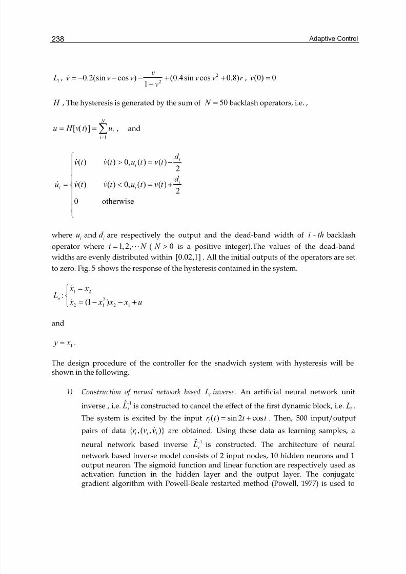
Adaptive Control238
i L , 2
20.2(sin cos ) (0.4 sin cos 0.8)
1
vv v v v v r
v= − − − + +
+& , (0) 0v =
H , The hysteresis is generated by the sum of 50 N = backlash operators, i.e. ,
1
[ ( )] N
i
i
u H v t u=
= =∑ , and
( ) ( ) 0, ( ) ( )2
( ) ( ) 0, ( ) ( )2
0 otherwise
i
i
ii i
d v t v t u t v t
d u v t v t u t v t
⎧> = −⎪
⎪⎪
= < = +⎨⎪⎪⎪⎩
& &
& & &
where iu and id are respectively the output and the dead-band width of i - th backlash
operator where 1, 2,i N = L ( 0 N > is a positive integer).The values of the dead-band
widths are evenly distributed within [0.02,1] . All the initial outputs of the operators are set
to zero. Fig. 5 shows the response of the hysteresis contained in the system.
o L :1 2
2
2 1 2 1(1 )
x x
x x x x u
=⎧⎨
= − − +⎩
&
&
and
1 y x= .
The design procedure of the controller for the snadwich system with hysteresis will beshown in the following.
1) Construction of nerual network based i L inverse. An artificial neural network unit
inverse , i.e. 1ˆi L− is constructed to cancel the effect of the first dynamic block, i.e. i L .
The system is excited by the input ( ) sin 2 cosl r t t t = + . Then, 500 input/output
pairs of data , ( , )l l l r v v& are obtained. Using these data as learning samples, a
neural network based inverse 1ˆi L− is constructed. The architecture of neural
network based inverse model consists of 2 input nodes, 10 hidden neurons and 1output neuron. The sigmoid function and linear function are respectively used asactivation function in the hidden layer and the output layer. The conjugategradient algorithm with Powell-Beale restarted method (Powell, 1977) is used to
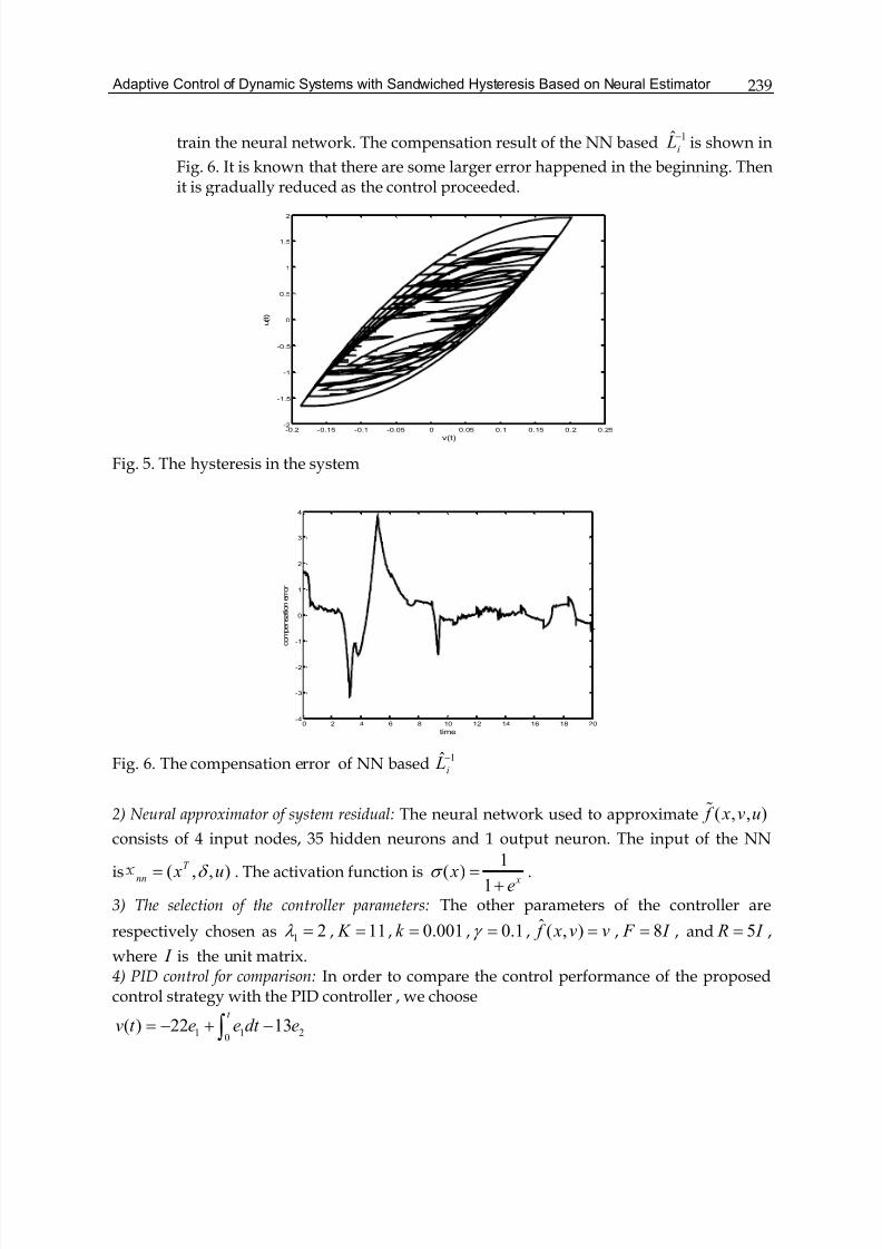
Adaptive Control of Dynamic Systems with Sandwiched Hysteresis Based on Neural Estimator 239
train the neural network. The compensation result of the NN based 1ˆi L− is shown in
Fig. 6. It is known that there are some larger error happened in the beginning. Thenit is gradually reduced as the control proceeded.
-0.2 -0.15 -0.1 -0.05 0 0.05 0.1 0.15 0.2 0.25-2
-1.5
-1
-0.5
0
0.5
1
1.5
2
v(t)
u ( t )
Fig. 5. The hysteresis in the system
0 2 4 6 8 10 12 14 16 18 20-4
-3
-2
-1
0
1
2
3
4
time
c o m p e n s a
t i o n e r r o r
Fig. 6. The compensation error of NN based 1ˆ
i L−
2) Neural approximator of system residual: The neural network used to approximate ( , , ) f x v u%
consists of 4 input nodes, 35 hidden neurons and 1 output neuron. The input of the NN
is ( , , )T
nn x uδ = . The activation function is1
( )1 x
xe
σ =+
.
3) The selection of the controller parameters: The other parameters of the controller are
respectively chosen as 1 2λ = , 11 K = , 0.001k = , 0.1γ = , ˆ ( , ) f x v v= , 8 F I = , and 5 R I = ,
where I is the unit matrix.4) PID control for comparison: In order to compare the control performance of the proposedcontrol strategy with the PID controller , we choose
1 1 20
( ) 22 13t
v t e e dt e= − + −∫
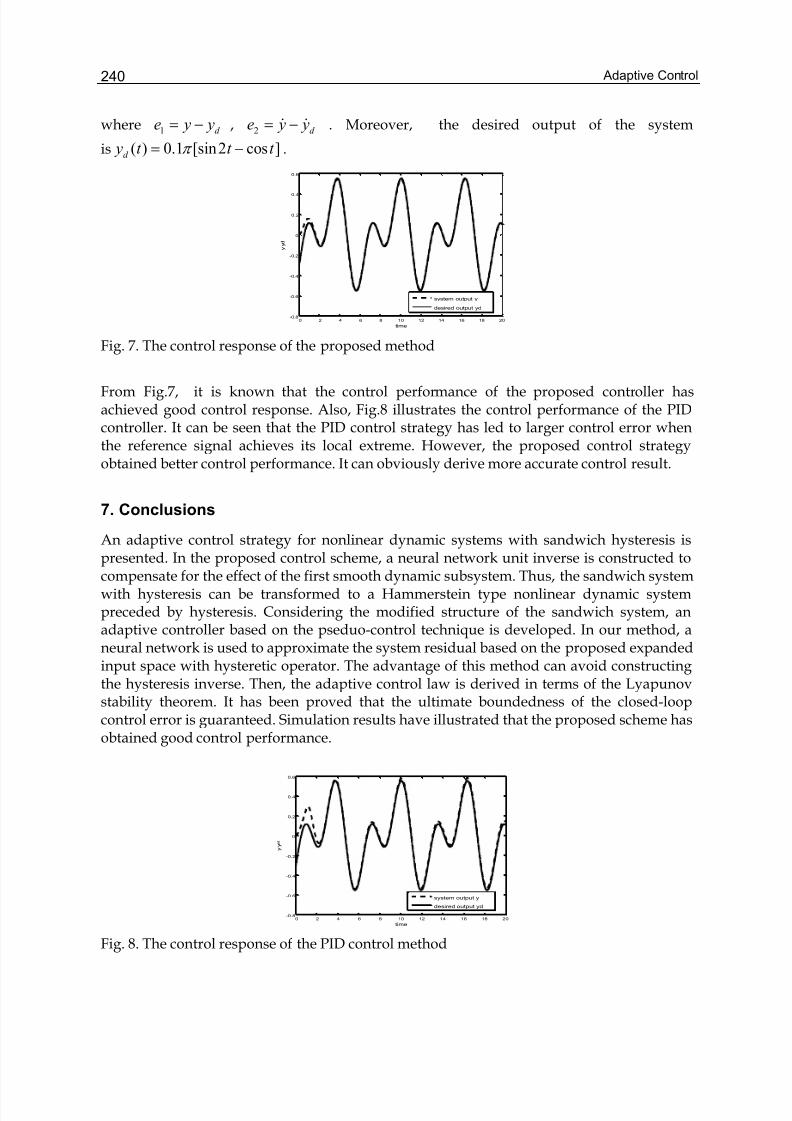
Adaptive Control240
where 1 d e y y= − , 2 d e y y= −& & . Moreover, the desired output of the system
is ( ) 0.1 [sin 2 cos ]d y t t t π = − .
0 2 4 6 8 10 12 14 16 18 20-0.8
-0.6
-0.4
-0.2
0
0.2
0.4
0.6
time
y y d
system output y
desired output yd
Fig. 7. The control response of the proposed method
From Fig.7, it is known that the control performance of the proposed controller hasachieved good control response. Also, Fig.8 illustrates the control performance of the PIDcontroller. It can be seen that the PID control strategy has led to larger control error whenthe reference signal achieves its local extreme. However, the proposed control strategyobtained better control performance. It can obviously derive more accurate control result.
7. Conclusions
An adaptive control strategy for nonlinear dynamic systems with sandwich hysteresis ispresented. In the proposed control scheme, a neural network unit inverse is constructed tocompensate for the effect of the first smooth dynamic subsystem. Thus, the sandwich systemwith hysteresis can be transformed to a Hammerstein type nonlinear dynamic systempreceded by hysteresis. Considering the modified structure of the sandwich system, anadaptive controller based on the pseduo-control technique is developed. In our method, aneural network is used to approximate the system residual based on the proposed expandedinput space with hysteretic operator. The advantage of this method can avoid constructingthe hysteresis inverse. Then, the adaptive control law is derived in terms of the Lyapunovstability theorem. It has been proved that the ultimate boundedness of the closed-loopcontrol error is guaranteed. Simulation results have illustrated that the proposed scheme hasobtained good control performance.
0 2 4 6 8 10 12 14 16 18 20-0.8
-0.6
-0.4
-0.2
0
0.2
0.4
0.6
time
y y d
system output y
desired output yd
Fig. 8. The control response of the PID control method
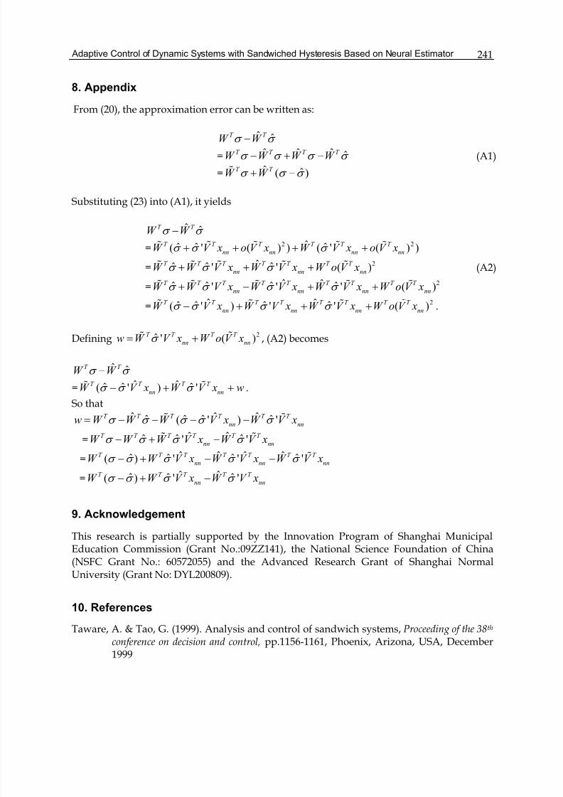
Adaptive Control of Dynamic Systems with Sandwiched Hysteresis Based on Neural Estimator 241
8. Appendix
From (20), the approximation error can be written as:
ˆ ˆT T W W −σ σ
= ˆ ˆ ˆ ˆT T T T W W W W − + −σ σ σ σ (A1)
= ˆ ˆ( )T T W W + −% σ σ σ
Substituting (23) into (A1), it yields
ˆ ˆT T W W −σ σ
= 2 2ˆˆ ˆ ˆ( ' ( ) ) ( ' ( ) )T T T T T T
nn nn nn nnW V x o V x W V x o V x+ + + +% % % % %σ σ σ
= 2ˆˆ ˆ ˆ' ' ( )T T T T T T T
nn nn nnW W V x W V x W o V x+ + +% % % % %σ σ σ (A2)
= 2ˆ ˆˆ ˆ ˆ ˆ' ' ' ( )T T T T T T T T T
nn nn nn nnW W V x W V x W V x W o V x+ − + +% % % % %σ σ σ σ
= 2ˆ ˆˆ ˆ ˆ ˆ( ' ) ' ' ( )T T T T T T T T
nn nn nn nnW V x W V x W V x W o V x− + + +% % % %σ σ σ σ .
Defining 2ˆ ' ( )T T T T
nn nnw W V x W o V x= +% %σ , (A2) becomes
ˆ ˆT T W W −σ σ
= ˆ ˆˆ ˆ ˆ( ' ) 'T T T T
nn nnW V x W V x w− + +% %σ σ σ .
So that
ˆ ˆ ˆˆ ˆ ˆ ˆ( ' ) 'T T T T T T
nn nnw W W W V x W V x= − − − −% %σ σ σ σ σ
= ˆ ˆˆ ˆ ˆ' 'T T T T T T
nn nnW W W V x W V x− + −% %σ σ σ σ
= ˆ ˆ ˆ ˆˆ ˆ ˆ ˆ( ) ' ' 'T T T T T T T
nn nn nnW W V x W V x W V x− + − − %σ σ σ σ σ
= ˆ ˆˆ ˆ ˆ( ) ' 'T T T T T
nn nnW W V x W V x− + −σ σ σ σ
9. Acknowledgement
This research is partially supported by the Innovation Program of Shanghai MunicipalEducation Commission (Grant No.:09ZZ141), the National Science Foundation of China(NSFC Grant No.: 60572055) and the Advanced Research Grant of Shanghai NormalUniversity (Grant No: DYL200809).
10. References
Taware, A. & Tao, G. (1999). Analysis and control of sandwich systems, Proceeding of the 38th conference on decision and control, pp.1156-1161, Phoenix, Arizona, USA, December1999
Adaptive Control242
Tao, G. & Ma, X.(2001).Optimal and nonlinear decoupling control of system withsandwiched backlash, Automatica, Vol.37, No.1, 165-176.
Hovakimyan, N.& Nandi, F.(2002). Adaptive output feedback control of uncertain nonlinearsystems using single-hidden-layer neural networks, IEEE Transactions on NeuralNetworks, Vol.13, No.6, 1420-1431
Calis, A.& Hovakimyan, N. (2001). Adaptive output feedback control of nonlinear systemsusing neural networks, Automatica, Vol. 37, 1201-1211.
Powell, M.(1977). Restart procedures for the conjugate gradient method, MathematicalProgramming, Vol. 12, 241-254.
Zhao, X.; Tan, Y. & Zhao, T.(2008). Adaptive control of nonlinear system with sandwichedhysteresis using Duhem operator, Control and Decision, Vol. 22, No. 10, 1134-1138
Corradini, M., Manni, A & Parlangeli, G. (2007). Variable structure control of nonlinearuncertain sandwich systems with nonsmooth nonlinearities,Proceedings of the 46thIEEE Conference on Decision and Control, pp. 2023-2038
Zhao, X. & Tan, Y.(2006). Neural adaptive control of dynamic sandwich systems withhysteresis, Proceedings of the 2006 IEEE International Symposium on Intelligent Control,pp. 82-87
Adly, A.A.& Abd-El-Hafiz, S.K. (1998). Using neural networks in the identification ofPreisach-type hysteresis models. IEEE Trans. on Magnetics, Vol. 34, No.3, 629-635
Zhao, X. & Tan, Y. (2008). Modeling hysteresis and its inverse model using neural networksbased on expanded input space method,IEEE Transactions on Control SystemsTechnology, Vol. 16, No. 3, pp. 484-490
11
High-Speed Adaptive Control Technique Basedon Steepest Descent Method for Adaptive
Chromatic Dispersion Compensation in OpticalCommunications
Ken Tanizawa and Akira HiroseDepartment of Electronic Engineering, The University of Tokyo
Japan
1. Introduction
The traffic volume of the data transmission is increasing each year with the explosivegrowth of the Internet. The networking technologies supporting the data transmission areoptical fiber transmission technologies. In the physical layer, the networks are classified intothree networks, the long-haul network that connects city to city, the metropolitan areanetwork that connects the central station in the city to the neighboring base station, and theaccess network that connects the base station to the home. In order to adapt to the increaseof the data transmission, we need to achieve high-speed transmission and increase thecapacity of transmission in each network.In the access network, many kinds of passive optical networks (PON) are studied to offer ahigh-speed access to the Internet at low cost. In the metropolitan area network, wecontemplate the update of the network structure from the conventional peer-to-peertransmission to the ring or mesh structure for the high-capacity and highly reliable networks.In the long-haul network, the study on multilevel modulation such as the differentialquadrature phase shift keying (DQPSK) is a recent popular topic for the high-capacitytransmission because the multilevel modulation utilizing the phase information offers high-speed transmission without increasing the symbol rate. Other modulation and multiplexingtechnologies are also studied for the high-capacity networks. The orthogonal frequencydivision multiplexing (OFDM) is one of the wavelength division multiplexing methods andachieves high spectral efficiency by the use of orthogonal carrier frequencies. The opticalcode division multiple access (OCDMA) is a multiplexing technique in the code domain.These techniques are developed in the wireless communication and modified for the opticaltransmission technologies in these days.In the long-haul and the metropolitan area networks whose transmission distance is over 10km in 40 Gb/s, chromatic dispersion (CD) is one of the main factors which limits thetransmission speed and the advances of the network structure. The CD is a physicalphenomenon that the group velocity of light in the fiber depends on its wavelength(Agrawal, 2002). The CD causes the degradation of the transmission quality as the optical
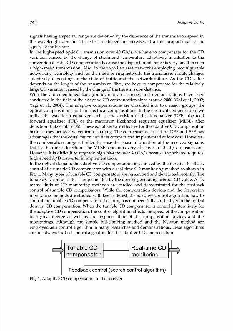
Adaptive Control244
signals having a spectral range are distorted by the difference of the transmission speed inthe wavelength domain. The effect of dispersion increases at a rate proportional to thesquare of the bit-rate.In the high-speed optical transmission over 40 Gb/s, we have to compensate for the CDvariation caused by the change of strain and temperature adaptively in addition to theconventional static CD compensation because the dispersion tolerance is very small in sucha high-speed transmission. Also, in metropolitan area networks employing reconfigurablenetworking technology such as the mesh or ring network, the transmission route changesadaptively depending on the state of traffic and the network failure. As the CD valuedepends on the length of the transmission fiber, we have to compensate for the relativelylarge CD variation caused by the change of the transmission distance.With the aforementioned background, many researches and demonstrations have beenconducted in the field of the adaptive CD compensation since around 2000 (Ooi et al., 2002;Yagi et al., 2004). The adaptive compensations are classified into two major groups, theoptical compensations and the electrical compensations. In the electrical compensation, weutilize the waveform equalizer such as the decision feedback equalizer (DFE), the feedforward equalizer (FFE) or the maximum likelihood sequence equalizer (MLSE) afterdetection (Katz et al., 2006). These equalizers are effective for the adaptive CD compensationbecause they act as a waveform reshaping. The compensation based on DEF and FFE hasadvantages that the equalization circuit is compact and implemented at low cost. However,the compensation range is limited because the phase information of the received signal islost by the direct detection. The MLSE scheme is very effective in 10 Gb/s transmission.However it is difficult to upgrade high bit-rate over 40 Gb/s because the scheme requireshigh-speed A/D converter in implementation.In the optical domain, the adaptive CD compensation is achieved by the iterative feedbackcontrol of a tunable CD compensator with a real-time CD monitoring method as shown inFig. 1. Many types of tunable CD compensators are researched and developed recently. Thetunable CD compensator is implemented by the devices generating arbitral CD value. Also,many kinds of CD monitoring methods are studied and demonstrated for the feedbackcontrol of tunable CD compensators. While the compensation devices and the dispersionmonitoring methods are studied with keen interest, the adaptive control algorithm, how tocontrol the tunable CD compensator efficiently, has not been fully studied yet in the opticaldomain CD compensation. When the tunable CD compensator is controlled iteratively forthe adaptive CD compensation, the control algorithm affects the speed of the compensationto a great degree as well as the response time of the compensation devices and themonitorings. Although the simple hill-climbing method and the Newton method areemployed as a control algorithm in many researches and demonstrations, these algorithmsare not always the best control algorithm for the adaptive CD compensation.
Tunable CD
compensator
Real-time CD
monitoring
Feedback control (search control algorithm)
Fig. 1. Adaptive CD compensation in the receiver.
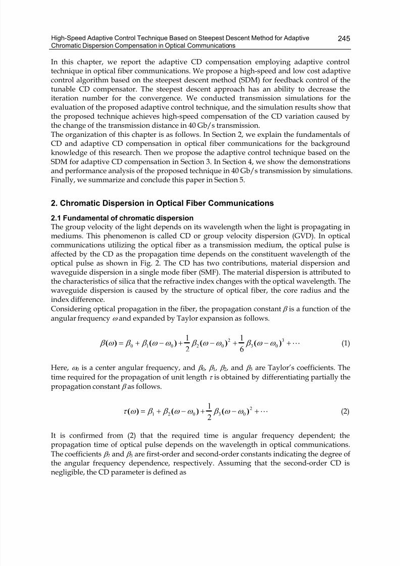
High-Speed Adaptive Control Technique Based on Steepest Descent Method for AdaptiveChromatic Dispersion Compensation in Optical Communications
245
In this chapter, we report the adaptive CD compensation employing adaptive controltechnique in optical fiber communications. We propose a high-speed and low cost adaptivecontrol algorithm based on the steepest descent method (SDM) for feedback control of thetunable CD compensator. The steepest descent approach has an ability to decrease theiteration number for the convergence. We conducted transmission simulations for theevaluation of the proposed adaptive control technique, and the simulation results show thatthe proposed technique achieves high-speed compensation of the CD variation caused bythe change of the transmission distance in 40 Gb/s transmission.The organization of this chapter is as follows. In Section 2, we explain the fundamentals ofCD and adaptive CD compensation in optical fiber communications for the backgroundknowledge of this research. Then we propose the adaptive control technique based on theSDM for adaptive CD compensation in Section 3. In Section 4, we show the demonstrationsand performance analysis of the proposed technique in 40 Gb/s transmission by simulations.Finally, we summarize and conclude this paper in Section 5.
2. Chromatic Dispersion in Optical Fiber Communications
2.1 Fundamental of chromatic dispersion
The group velocity of the light depends on its wavelength when the light is propagating inmediums. This phenomenon is called CD or group velocity dispersion (GVD). In opticalcommunications utilizing the optical fiber as a transmission medium, the optical pulse isaffected by the CD as the propagation time depends on the constituent wavelength of theoptical pulse as shown in Fig. 2. The CD has two contributions, material dispersion andwaveguide dispersion in a single mode fiber (SMF). The material dispersion is attributed tothe characteristics of silica that the refractive index changes with the optical wavelength. Thewaveguide dispersion is caused by the structure of optical fiber, the core radius and theindex difference.
Considering optical propagation in the fiber, the propagation constant β is a function of the
angular frequency ω and expanded by Taylor expansion as follows.
L+−+−+−+= 3
03
2
02010
6
1
2
1)()()()( ω ω β ω ω β ω ω β β ω β (1)
Here, ω 0 is a center angular frequency, and β 0, β 1, β 2, and β 3 are Taylor’s coefficients. The
time required for the propagation of unit length τ is obtained by differentiating partially the
propagation constant β as follows.
L+−+−+= 2
03021
2
1)()()( ω ω β ω ω β β ω τ (2)
It is confirmed from (2) that the required time is angular frequency dependent; thepropagation time of optical pulse depends on the wavelength in optical communications.
The coefficients β 2 and β 3 are first-order and second-order constants indicating the degree ofthe angular frequency dependence, respectively. Assuming that the second-order CD isnegligible, the CD parameter is defined as
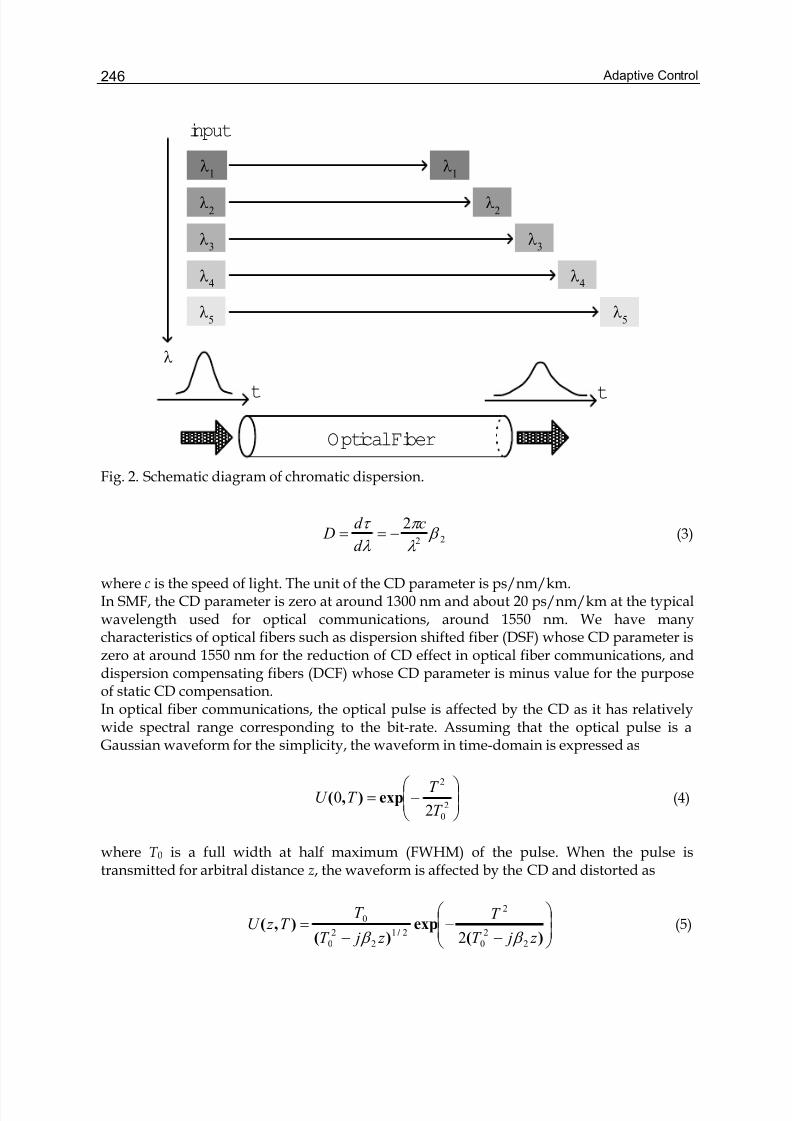
Adaptive Control246
λ1
λ2
λ3
λ4
λ5
input
λ1
λ2
λ3
λ4
λ5
λ
Optical Fiber
t t
Fig. 2. Schematic diagram of chromatic dispersion.
22
2 β
λ
π
λ
τ c
d
d D −== (3)
where c is the speed of light. The unit of the CD parameter is ps/nm/km.In SMF, the CD parameter is zero at around 1300 nm and about 20 ps/nm/km at the typicalwavelength used for optical communications, around 1550 nm. We have manycharacteristics of optical fibers such as dispersion shifted fiber (DSF) whose CD parameter iszero at around 1550 nm for the reduction of CD effect in optical fiber communications, anddispersion compensating fibers (DCF) whose CD parameter is minus value for the purposeof static CD compensation.In optical fiber communications, the optical pulse is affected by the CD as it has relativelywide spectral range corresponding to the bit-rate. Assuming that the optical pulse is aGaussian waveform for the simplicity, the waveform in time-domain is expressed as
⎟⎟ ⎠
⎞⎜⎜⎝
⎛ −=
2
0
2
20
T
T T U exp),( (4)
where T 0 is a full width at half maximum (FWHM) of the pulse. When the pulse istransmitted for arbitral distance z, the waveform is affected by the CD and distorted as
⎟⎟
⎠
⎞
⎜⎜
⎝
⎛
−−
−=
)(exp
)(),(
/ z jT
T
z jT
T T z U
2
2
0
2
21
2
2
0
0
2 β β (5)
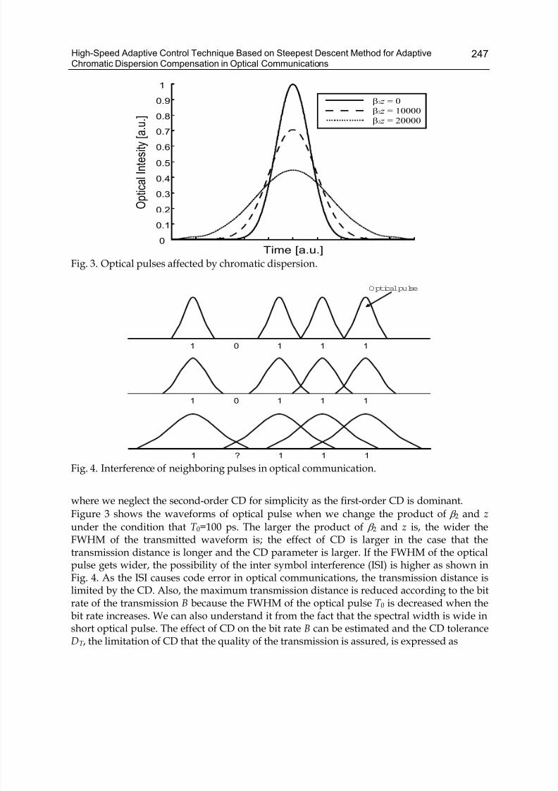
High-Speed Adaptive Control Technique Based on Steepest Descent Method for AdaptiveChromatic Dispersion Compensation in Optical Communications
247
x 105
0
0.1
0.2
0.3
0.4
0.5
0.6
0.7
0.8
0.9
1
Time [a.u.]
O p t i c a l I n t e s i t y [ a . u . ]
β2 z = 0
β2 z = 10000
β2 z = 20000
Fig. 3. Optical pulses affected by chromatic dispersion.
1 1 1 10
1 1 1 10
1 1 1 1?
Optical pulse
Fig. 4. Interference of neighboring pulses in optical communication.
where we neglect the second-order CD for simplicity as the first-order CD is dominant.
Figure 3 shows the waveforms of optical pulse when we change the product of β 2 and z
under the condition that T 0=100 ps. The larger the product of β 2 and z is, the wider theFWHM of the transmitted waveform is; the effect of CD is larger in the case that thetransmission distance is longer and the CD parameter is larger. If the FWHM of the opticalpulse gets wider, the possibility of the inter symbol interference (ISI) is higher as shown inFig. 4. As the ISI causes code error in optical communications, the transmission distance islimited by the CD. Also, the maximum transmission distance is reduced according to the bitrate of the transmission B because the FWHM of the optical pulse T 0 is decreased when thebit rate increases. We can also understand it from the fact that the spectral width is wide inshort optical pulse. The effect of CD on the bit rate B can be estimated and the CD toleranceDT , the limitation of CD that the quality of the transmission is assured, is expressed as
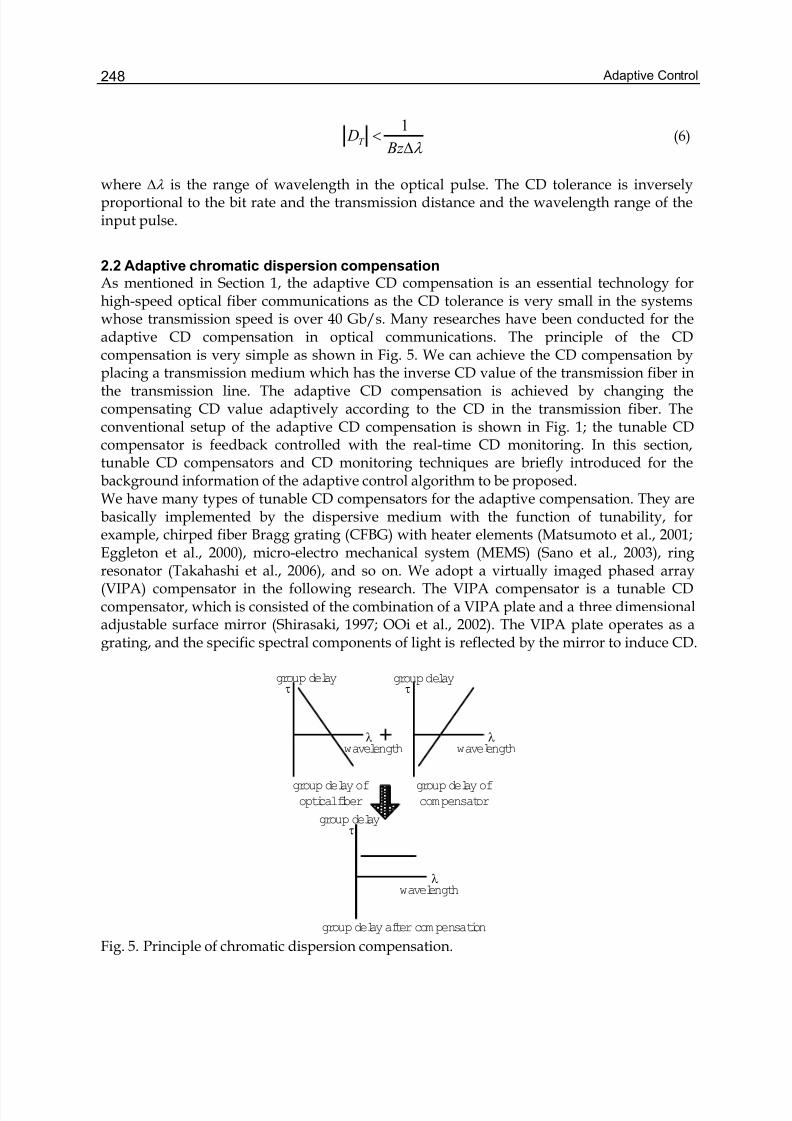
Adaptive Control248
λ Δ<
Bz DT
1 (6)
where Δλ is the range of wavelength in the optical pulse. The CD tolerance is inverselyproportional to the bit rate and the transmission distance and the wavelength range of theinput pulse.
2.2 Adaptive chromatic dispersion compensationAs mentioned in Section 1, the adaptive CD compensation is an essential technology forhigh-speed optical fiber communications as the CD tolerance is very small in the systemswhose transmission speed is over 40 Gb/s. Many researches have been conducted for theadaptive CD compensation in optical communications. The principle of the CDcompensation is very simple as shown in Fig. 5. We can achieve the CD compensation byplacing a transmission medium which has the inverse CD value of the transmission fiber inthe transmission line. The adaptive CD compensation is achieved by changing thecompensating CD value adaptively according to the CD in the transmission fiber. Theconventional setup of the adaptive CD compensation is shown in Fig. 1; the tunable CDcompensator is feedback controlled with the real-time CD monitoring. In this section,tunable CD compensators and CD monitoring techniques are briefly introduced for thebackground information of the adaptive control algorithm to be proposed.We have many types of tunable CD compensators for the adaptive compensation. They arebasically implemented by the dispersive medium with the function of tunability, forexample, chirped fiber Bragg grating (CFBG) with heater elements (Matsumoto et al., 2001;Eggleton et al., 2000), micro-electro mechanical system (MEMS) (Sano et al., 2003), ringresonator (Takahashi et al., 2006), and so on. We adopt a virtually imaged phased array(VIPA) compensator in the following research. The VIPA compensator is a tunable CDcompensator, which is consisted of the combination of a VIPA plate and a three dimensionaladjustable surface mirror (Shirasaki, 1997; OOi et al., 2002). The VIPA plate operates as agrating, and the specific spectral components of light is reflected by the mirror to induce CD.
group delay of
compensator
wavelength
τ
λ
group delay of
optical fiber
group delay after compensation
group delayτ
group delay
wavelength λ
τgroup delay
wavelength λ
Fig. 5. Principle of chromatic dispersion compensation.
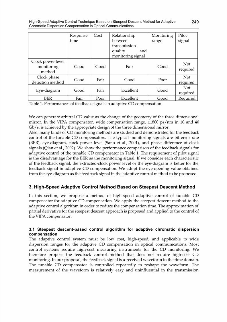
High-Speed Adaptive Control Technique Based on Steepest Descent Method for AdaptiveChromatic Dispersion Compensation in Optical Communications
249
Responsetime
Cost Relationshipbetweentransmissionquality andmonitoring signal
Monitoringrange
Pilotsignal
Clock power levelmonitoring
methodGood Good Fair Good
Notrequired
Clock phasedetection method
Good Fair Good PoorNot
required
Eye-diagram Good Fair Excellent GoodNot
required
BER Fair Poor Excellent Good Required
Table 1. Performances of feedback signals in adaptive CD compensation
We can generate arbitral CD value as the change of the geometry of the three dimensionalmirror. In the VIPA compensator, wide compensation range, ±1800 ps/nm in 10 and 40Gb/s, is achieved by the appropriate design of the three dimensional mirror.Also, many kinds of CD monitoring methods are studied and demonstrated for the feedbackcontrol of the tunable CD compensators. The typical monitoring signals are bit error rate(BER), eye-diagram, clock power level (Sano et al., 2001), and phase difference of clocksignals (Qian et al., 2002). We show the performance comparison of the feedback signals foradaptive control of the tunable CD compensator in Table 1. The requirement of pilot signalis the disadvantage for the BER as the monitoring signal. If we consider each characteristicof the feedback signal, the extracted-clock power level or the eye-diagram is better for thefeedback signal in adaptive CD compensation. We adopt the eye-opening value obtainedfrom the eye-diagram as the feedback signal in the adaptive control method to be proposed.
3. High-Speed Adaptive Control Method Based on Steepest Descent Method
In this section, we propose a method of high-speed adaptive control of tunable CDcompensator for adaptive CD compensation. We apply the steepest descent method to theadaptive control algorithm in order to reduce the compensation time. The approximation ofpartial derivative for the steepest descent approach is proposed and applied to the control ofthe VIPA compensator.
3.1 Steepest descent-based control algorithm for adaptive chromatic dispersioncompensationThe adaptive control system must be low cost, high-speed, and applicable to widedispersion ranges for the adaptive CD compensation in optical communications. Mostcontrol systems require high-cost measuring instruments for the CD monitoring. Wetherefore propose the feedback control method that does not require high-cost CDmonitoring. In our proposal, the feedback signal is a received waveform in the time domain.The tunable CD compensator is controlled repeatedly to reshape the waveform. Themeasurement of the waveform is relatively easy and uninfluential in the transmission
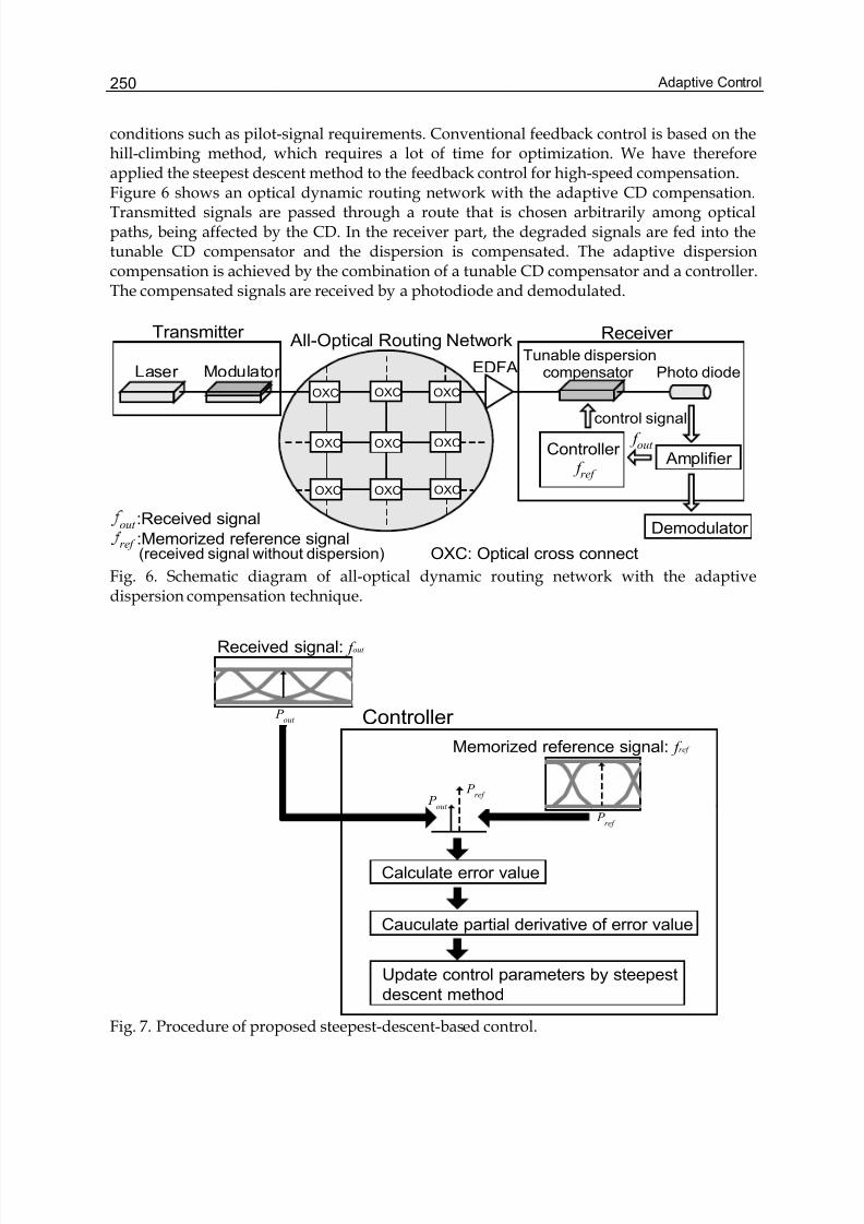
Adaptive Control250
conditions such as pilot-signal requirements. Conventional feedback control is based on thehill-climbing method, which requires a lot of time for optimization. We have thereforeapplied the steepest descent method to the feedback control for high-speed compensation.Figure 6 shows an optical dynamic routing network with the adaptive CD compensation.Transmitted signals are passed through a route that is chosen arbitrarily among opticalpaths, being affected by the CD. In the receiver part, the degraded signals are fed into thetunable CD compensator and the dispersion is compensated. The adaptive dispersioncompensation is achieved by the combination of a tunable CD compensator and a controller.The compensated signals are received by a photodiode and demodulated.
out :Received signal
ref :Memorized reference signal(received signal without dispersion)
Laser Modulator
Transmitter
Photo diode
Receiver
Amplifier
Demodulator
Tunable dispersioncompensator
Controller
EDFA
f out
f ref
control signal
All-Optical Routing Network
OXC
OXC
OXC
OXC
OXC
OXC
OXC
OXC
OXC
OXC: Optical cross connect Fig. 6. Schematic diagram of all-optical dynamic routing network with the adaptivedispersion compensation technique.
Memorized reference signal: f ref
Cauculate partial derivative of error value
Update control parameters by steepest
descent method
Received signal: f out
P out
P ref
Calculate error value
P out
P ref
Controller
Fig. 7. Procedure of proposed steepest-descent-based control.
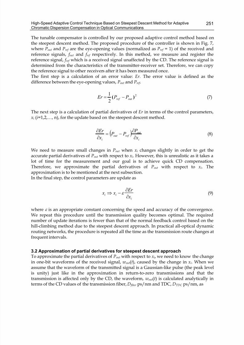
High-Speed Adaptive Control Technique Based on Steepest Descent Method for AdaptiveChromatic Dispersion Compensation in Optical Communications
251
The tunable compensator is controlled by our proposed adaptive control method based onthe steepest descent method. The proposed procedure of the controller is shown in Fig. 7,where Pout and Pref are the eye-opening values (normalized as Pref = 1) of the received andreference signals, f out and f ref respectively. In this method, we measure and register thereference signal, f ref which is a received signal unaffected by the CD. The reference signal isdetermined from the characteristics of the transmitter-receiver set. Therefore, we can copythe reference signal to other receivers after it has been measured once.The first step is a calculation of an error value: Er. The error value is defined as thedifference between the eye-opening values, Pout and Pref .
2
2
1)( out ref P P Er −= (7)
The next step is a calculation of partial derivatives of Er in terms of the control parameters,xi (i=1,2,…, n), for the update based on the steepest descent method.
( )i
out ref out
i x
P P P
x
Er
∂
∂−=
∂
∂(8)
We need to measure small changes in Pout when xi changes slightly in order to get theaccurate partial derivatives of Pout with respect to xi. However, this is unrealistic as it takes alot of time for the measurement and our goal is to achieve quick CD compensation.Therefore, we approximate the partial derivatives of Pout with respect to xi. Theapproximation is to be mentioned at the next subsection.In the final step, the control parameters are update as
i
ii x
Er x x
∂
∂−⇒ ε (9)
where ε is an appropriate constant concerning the speed and accuracy of the convergence.We repeat this procedure until the transmission quality becomes optimal. The requirednumber of update iterations is fewer than that of the normal feedback control based on thehill-climbing method due to the steepest descent approach. In practical all-optical dynamicrouting networks, the procedure is repeated all the time as the transmission route changes atfrequent intervals.
3.2 Approximation of partial derivatives for steepest descent approachTo approximate the partial derivatives of Pout with respect to xi, we need to know the changein one-bit waveforms of the received signal, wout(t), caused by the change in xi. When weassume that the waveform of the transmitted signal is a Gaussian-like pulse (the peak levelis unity) just like in the approximation in return-to-zero transmissions and that thetransmission is affected only by the CD, the waveform, wout(t) is calculated analytically interms of the CD values of the transmission fiber, D fiber ps/nm and TDC, DTDC ps/nm, as
Adaptive Control252
⎟⎟
⎠
⎞
⎜⎜
⎝
⎛ −=
2
22
FWHM
peak
peak out T
t vvt w exp)( (10)
222
2
2
2
22⎟⎟ ⎠
⎞⎜⎜⎝
⎛ ++
=
TDC fiber FWHM
FWHM peak
Dc
Dc
T
T v
π
λ
π
λ (11)
where T FWHM is the FWHM of the transmitted signal, λ is the center wavelength , t is time,and c is the speed of light. The partial derivative of wout(t) with respect to xi is calculatedfrom (10) and (11).
i
TDC
FWHM
peak
FWHM
peak
peak
FWHM
peak
i
out
x
D
cT
vt
T
vt v
T
v
x
t w
∂
∂⋅
⎟⎟
⎠
⎞
⎜⎜
⎝
⎛ −
⎟⎟
⎠
⎞
⎜⎜
⎝
⎛ −−±=
∂
∂
π
λ
21
21
2
2
22
2
22
2
2
2
exp)(
(12)
Equation (10) shows that the value v peak is the peak level of wout(t). We can measure it in apractical system. Therefore, (12) shows that we can obtain the approximated partial
derivative of wout(t) with respect to xi because T FWHM and λ are known parameters. We obtainthe partial derivative of the peak value in wout(t) by substituting 0 for t.
i
TDC peak
FWHM
peak
i
peak
t i
out
x
D
cv
T
v
x
v
x
t w
∂
∂⋅−±=
∂
∂=
∂
∂
=π
λ
21
2
2
2
2
0
)( (13)
The value of v peak corresponds to the eye-opening value in nonreturn-to-zero (NRZ)transmission approximately. Therefore, the partial derivative of Pout with respect to xi isapproximated as follows.
i
TDC out
FWHM
out
i
out
x
D
c P
T
P
x
P
∂
∂⋅−±=
∂
∂
π
λ
21
2
2
2
2
(14)
3.3 Detailed control algorithm for VIPA compensator In the simulations described in the next section, we employ a VIPA compensator as thetunable CD compensator. The VIPA compensator has a single control parameter, i.e. CD S ps/nm. The detailed control procedure of the VIPA compensator is as follows. In general,we can apply the proposed method to any kind of tunable CD compensators.
(i) Initialize the parameter of the VIPA compensator: S ps/nm
0=S ps/nm (15)
(ii) Calculate the error value: Er
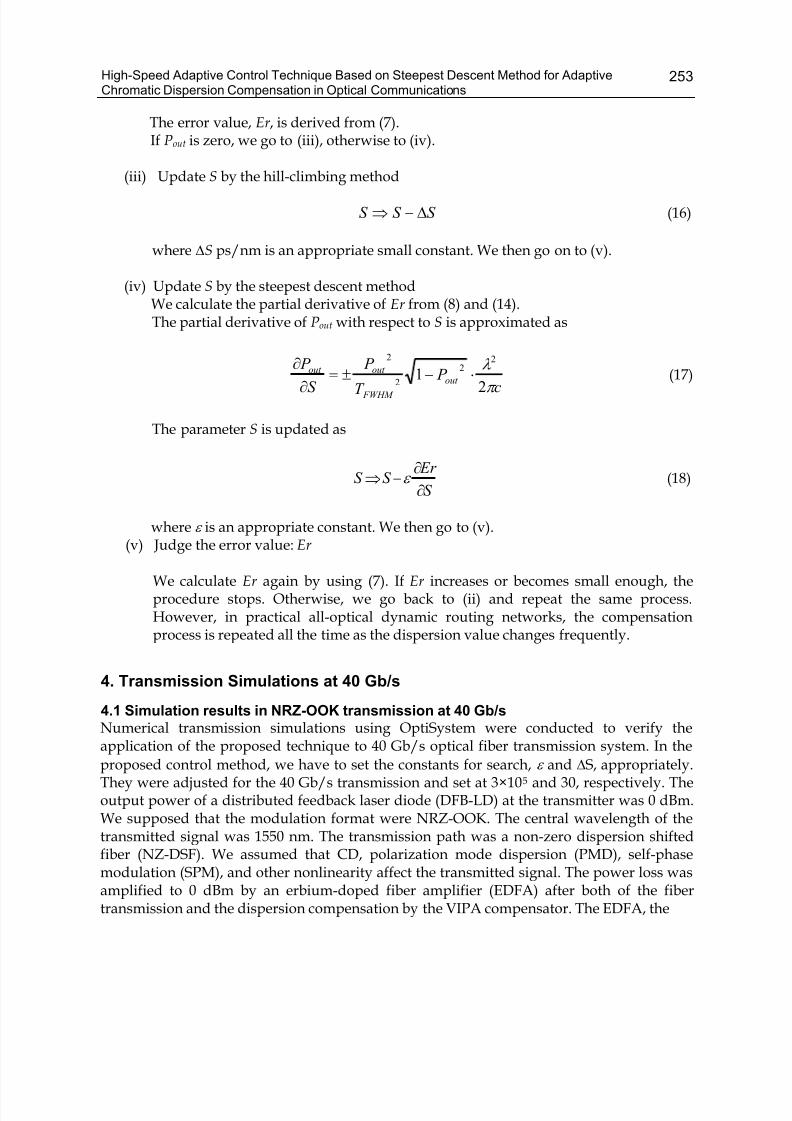
High-Speed Adaptive Control Technique Based on Steepest Descent Method for AdaptiveChromatic Dispersion Compensation in Optical Communications
253
The error value, Er , is derived from (7).If Pout is zero, we go to (iii), otherwise to (iv).
(iii) Update S by the hill-climbing method
S S S Δ−⇒ (16)
where ΔS ps/nm is an appropriate small constant. We then go on to (v).
(iv) Update S by the steepest descent methodWe calculate the partial derivative of Er from (8) and (14).The partial derivative of Pout with respect to S is approximated as
c P
T
P
S
P out
FWHM
out out
π
λ
21
2
2
2
2
⋅−±=∂
∂(17)
The parameter S is updated as
S
Er S S
∂
∂−⇒ ε (18)
where ε is an appropriate constant. We then go to (v).(v) Judge the error value: Er
We calculate Er again by using (7). If Er increases or becomes small enough, theprocedure stops. Otherwise, we go back to (ii) and repeat the same process.However, in practical all-optical dynamic routing networks, the compensationprocess is repeated all the time as the dispersion value changes frequently.
4. Transmission Simulations at 40 Gb/s
4.1 Simulation results in NRZ-OOK transmission at 40 Gb/sNumerical transmission simulations using OptiSystem were conducted to verify theapplication of the proposed technique to 40 Gb/s optical fiber transmission system. In the
proposed control method, we have to set the constants for search, ε and ΔS, appropriately.They were adjusted for the 40 Gb/s transmission and set at 3×10⁵ and 30, respectively. Theoutput power of a distributed feedback laser diode (DFB-LD) at the transmitter was 0 dBm.We supposed that the modulation format were NRZ-OOK. The central wavelength of thetransmitted signal was 1550 nm. The transmission path was a non-zero dispersion shiftedfiber (NZ-DSF). We assumed that CD, polarization mode dispersion (PMD), self-phasemodulation (SPM), and other nonlinearity affect the transmitted signal. The power loss wasamplified to 0 dBm by an erbium-doped fiber amplifier (EDFA) after both of the fibertransmission and the dispersion compensation by the VIPA compensator. The EDFA, the
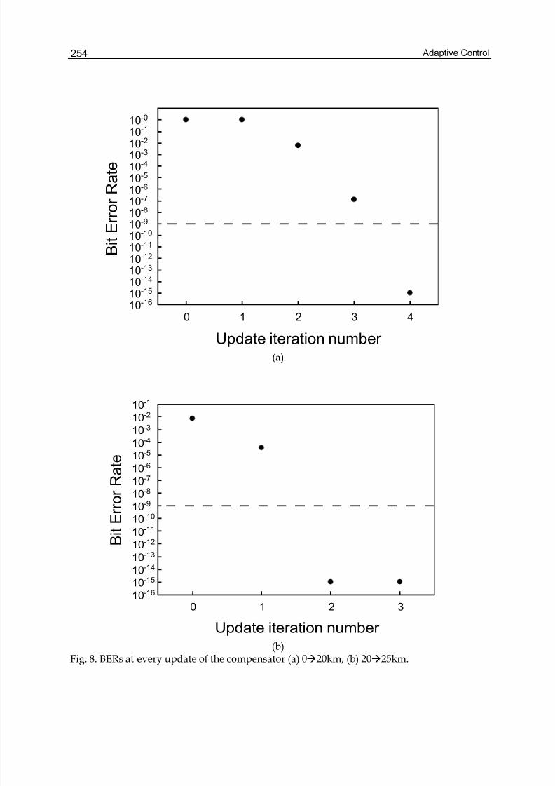
Adaptive Control254
Update iteration number
0 1 2 3 4
B i t E
r r o r
R a
t e
10-1610-1510-1410-1310-1210-1110-1010-910-810-710-610-510-410-310-210-110-0
(a)
Update iteration number
0 1 2 3
B i t E r r o r
R a
t e
10-16
10-15
10-14
10-13
10-12
10-11
10-10
10-910-8
10-7
10-6
10-5
10-4
10-3
10-2
10-1
(b)
Fig. 8. BERs at every update of the compensator (a) 0Æ20km, (b) 20Æ25km.
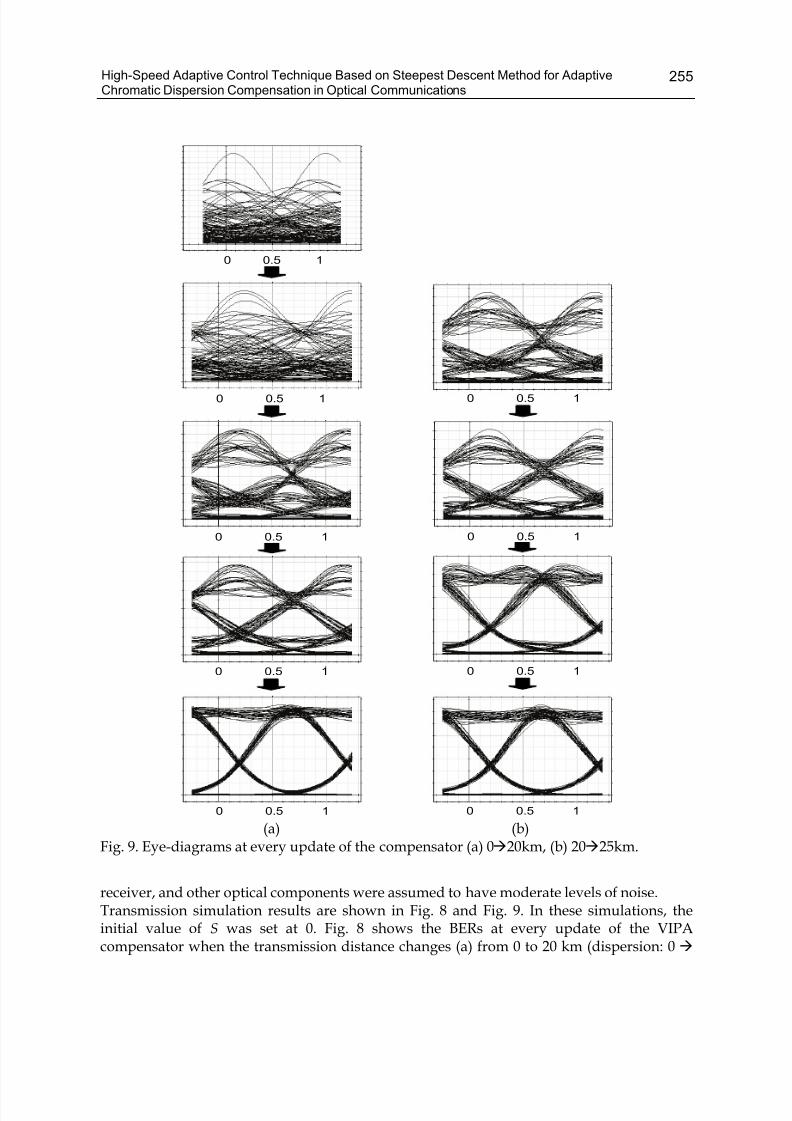
High-Speed Adaptive Control Technique Based on Steepest Descent Method for AdaptiveChromatic Dispersion Compensation in Optical Communications
255
0 0.5 1
0 0.5 1
0 0.5 1
0 0.5 1
0 0.5 1 0 0.5 1
0 0.5 1
0 0.5 1
0 0.5 1
(a) (b)
Fig. 9. Eye-diagrams at every update of the compensator (a) 0Æ20km, (b) 20Æ25km.
receiver, and other optical components were assumed to have moderate levels of noise.Transmission simulation results are shown in Fig. 8 and Fig. 9. In these simulations, theinitial value of S was set at 0. Fig. 8 shows the BERs at every update of the VIPAcompensator when the transmission distance changes (a) from 0 to 20 km (dispersion: 0Æ
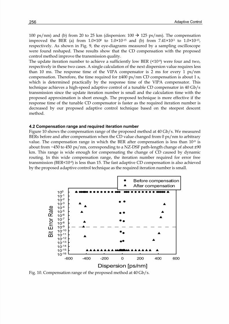
Adaptive Control256
100 ps/nm) and (b) from 20 to 25 km (dispersion: 100 Æ 125 ps/nm). The compensationimproved the BER (a) from 1.0×100 to 1.0×10⁻¹⁵ and (b) from 7.41×10⁻³ to 1.0×10⁻¹⁵,respectively. As shown in Fig. 9, the eye-diagrams measured by a sampling oscilloscopewere found reshaped. These results show that the CD compensation with the proposedcontrol method improve the transmission quality.The update iteration number to achieve a sufficiently low BER (<10-9) were four and two,respectively in these two cases. A single calculation of the next dispersion value requires lessthan 10 ms. The response time of the VIPA compensator is 2 ms for every 1 ps/nmcompensation. Therefore, the time required for ±400 ps/nm CD compensation is about 1 s,which is determined practically by the response time of the VIPA compensator. Thistechnique achieves a high-speed adaptive control of a tunable CD compensator in 40 Gb/stransmission since the update iteration number is small and the calculation time with theproposed approximation is short enough. The proposed technique is more effective if theresponse time of the tunable CD compensator is faster as the required iteration number isdecreased by our proposed adaptive control technique based on the steepest descentmethod.
4.2 Compensation range and required iteration number
Figure 10 shows the compensation range of the proposed method at 40 Gb/s. We measuredBERs before and after compensation when the CD value changed from 0 ps/nm to arbitraryvalue. The compensation range in which the BER after compensation is less than 10-9 isabout from −450 to 450 ps/nm, corresponding to a NZ-DSF path-length change of about ±90km. This range is wide enough for compensating the change of CD caused by dynamicrouting. In this wide compensation range, the iteration number required for error freetransmission (BER<10-9) is less than 15. The fast adaptive CD compensation is also achievedby the proposed adaptive control technique as the required iteration number is small.
Dispersion [ps/nm]
-600 -400 -200 0 200 400 600
B i t E r r o r R a t e
10-1610-1510-1410-1310-1210-1110-1010-910-810-710-610-510-410-310-210-1100
Before compensation
After compensation
Fig. 10. Compensation range of the proposed method at 40 Gb/s.
High-Speed Adaptive Control Technique Based on Steepest Descent Method for AdaptiveChromatic Dispersion Compensation in Optical Communications
257
5. Conclusion
In this chapter, we have proposed high-speed adaptive CD compensation with the adaptivecontrol method based on the steepest descent method and reported the performancesevaluated by numerical simulations.The simulation results show that the proposed control method based on the steepest descentmethod controls the tunable CD compensator quickly and effectively for a wide dispersionrange in 40 Gb/s transmission. The range is up to ±450 ps/nm, and the requiredcompensation time is about 1 s for the CD variation within ±400 ps/nm at 40 Gb/s. Theseachievements are valuable for the future optical networks employing dynamic routingtechnique.
6. References
Agrawal, G. (2002). Fiber-Optic Communication Systems, Wiley-Interscience, ISBN 0-471-21571-6, USA
Eggleton, B. J.; Ahuja, A.; Westbrook, P. S.; Rogers, J. A.; Kuo, P.; Nielsen, T. N. & Mikkelsen,B. (2000). Integrated Tunable Fiber Gratings for Dispersion Management in High-Bit Rate Systems. IEEE/OSA Journal of Lightwave Technology, Vol. 18, No. 10, (Oct.2000) pp. 1418-1432
Katz, G.; Sadot, D. & Tabrikian , J. (2006). Electrical Dispersion Compensation Equalizers inOptical Direct- and Coherent-Detection Systems. IEEE Transanctions onCommunications, Vol. 54, No. 11, (Nov. 2006) pp. 2045-2050
Matsumoto, S.; Ohira, T.; Takabayashi, M.; Yoshiara, K. & Sugihara, T. (2001). TunableDispersion Equalizer with a Divided Thin-Film Heater for 40-Gb/s RZTransmission. IEEE Photonics Technology Letters, Vol. 13, (Aug. 2001) pp. 827-829
Ooi, H.; Nakamura, K.; Akiyama, Y.; Takahara, T.; Terahara, T.; Kawahata, Y.; Isono, H. &Ishikawa, G. (2002). 40-Gb/s WDM Transmission With Virtually Imaged PhasedArray (VIPA) Variable Dispersion Compensators. IEEE/OSA Journal of LightwaveTechnology, Vol. 20, (Dec. 2002) pp. 2196-2203
Sano, T.; Iwashima, T.; Katayama, M.; Kanie, T.; Harumoto, M.; Shigehara, M.; Suganuma,H.; & Nishimura, M. (2003). Novel Multichannel Tunable Chromatic DispersionCompensator Based on MEMS and Diffraction Grating. IEEE Photonics TechnologyLetters, Vol. 15, No. 8, (Aug. 2003) pp. 1109-1111
Shirasaki, M. (1997). Chromatic-Dispersion Compensator Using Virtually Imaged PhasedArray. IEEE Photonics Technology Letters, Vol. 9, No. 12, (Dec. 1997) pp. 1598-1600
Tanizawa, K. & Hirose, A. (2007). Adaptive Control of Tunable Dispersion CompensatorThat Minimizes Time-Domain Waveform Error by Steepest Descent Method. IEEEPhotonics Technology Letters, Vol. 18, No. 13, (Jul. 2006) pp. 1466-1468
Tanizawa, K. & Hirose, A. (2007). Performance Analysis of Steepest-Descent-BasedFeedback Control of Tunable Dispersion Compensator for Adaptive DispersionCompensation in All-Optical Dynamic Routing Networks. IEEE/OSA Journal of Lightwave Technology, Vol. 24, No. 4, (Apr. 2007) pp. 1086-1094
Yagi, M.; Satomi, S.; Tanaka, S.; Ryu, S.; & Asano, S. (2005). Field Trial of AutomaticChromatic Dispersion Compensation for 40-Gb/s-Based Wavelength Path

Adaptive Control258
Protection. IEEE Photonics Technology Letters, Vol. 17, No. 1, (Jan. 2005) pp. 229-231
12
Adaptive Control of Piezoelectric Actuatorswith Unknown Hysteresis
Wen-Fang Xie, Jun Fu, Han Yao and, C.-Y. SuDepartment of Mechanical & Industrial Engineering
Concordia UniversityCanada
1. Introduction
Hysteresis phenomenon occurs in all smart material-based sensors and actuators, such asshape memory alloys, piezoceramics and magnetostrictive actuators (Bank & Smith, 2000;Tan & Baras, 2004). In order to study this phenomenon, different models were proposed(Brokate & Sprekels, 1996; Visintin, 1994). Normally, hysteresis models are classified intotwo categories, physics-based model such as Jiles-Atherton model (Jiles & Atherton, 1986)and phenomenology-based model such as Preisach operator (Brokate & Sprekels, 1996;Visintin, 1994) and Duhem model (Visintin, 1994). From control systems point of view,hysteresis is generally non-differentiable, nonlinear, and unknown. As a result, systemswith hysteresis usually exhibit undesirable inaccuracies or oscillation and even instability.Mitigating the effect of hysteresis becomes necessary and important, thus it has receivedincreasing attention in recent years (Tao & Kokotovic, 1995, Su, et al, 2000, Su, et al, 2005).Many of these studies are related to modeling of hysteresis and their control issues.With the development of artificial intelligent (AI), AI is being applied to dealing withnonlinearities in systems (Ge & Wang, 2002). Only a few studies have been carried out byusing NN to tackle hysteresis modeling and compensation (Makaveev, et al, 2002;Kuczmann & Ivanyi, 2002; Beuschel et al, 1998; Zhao & Tan, 2006). In the paper (Makaveev,et al, 2002), a NN model is used to describe the hysteresis behavior in different frequencieswith the knowledge of some properties of magnetic materials, such as loss separationproperty to allow the separate treatment of quasi-static and dynamic hysteretic effects.Beuschel et al used (Beuschel et al, 1998) a modified Luenberger observer and NN are usedto identify a general model of hysteresis. These researches demonstrate that NN can work asan unknown function approximator to describe the characteristics of hysteresis. Recently,two papers (Zhao & Tan, 2006; Lin et al 2006) applied the approximation property of NN tocoping with the identification of Preisach-type hysteresis in piezoelectric actuator, and thehysteresis estimation problem for piezo-positioning mechanism based on hysteresis frictionforce function, respectively. It should be noted that the aforementioned results share acommon assumption that the output of hysteresis is measurable.In practical systems, smart actuators are integrated into the systems, which makes themeasurement of output of hysteresis hard. Hence it is a challenge to design an observer for
Adaptive Control260
the unavailable output of hysteresis. Due to the unavailability of the output of hysteresis,the major obstacle of pre-inversion compensator for hysteresis is the lack of effectiveobserver design methods for piezoelectric actuators. Especially, the traditional “Luenberger-type” nonlinear observer design (Krener & Isidori, 1983) or the “high-gain” observer(Krener & Kang, 2003) cannot be applied directly, since the hysteresis is highly nonlinear.The sliding-mode observer was developed to estimate the internal friction states of LuGremodel for the servo actuators with friction (Xie, 2007). This observer needs a low-pass filterto remove the high-frequency components in the estimated state variable, which is notapplicable in this paper. Yang and Lin (Yang & Lin, 2004) proposed homogeneousobservers design for a class of n-dimensional inherently nonlinear systems whose Jacobianlinearization is neither controllable nor observable.Inspired by NN’s universal approximation property, and the aforementioned facts inobserver design, we propose an observer-based adaptive control of piezoelectric actuatorswith unknown hysteresis in this paper. The main contribution of this paper is the following:First, it applies the NN to on-line approximate complicated piecewise continuous unknownnonlinear functions in the explicit solution to Duhem model. Second, an observer isdesigned to estimate the output of hysteresis of piezoelectric actuator based on the systeminput and output. Third, the stability of the controlled piezoelectric actuator with theobserver is guaranteed by using Lyapunov extension (Kuczmann & Ivanyi, 2002).The organization of the paper is as follows. In Section II, a Duhem model of hysteresis andthe problem statement are given. The main results on NN-based compensator for hysteresisare presented in Section III. Section IV provides an example to show the feasibility of theproposed method. Conclusions are given in Section V.
2. Preliminaries
2.1 Duhem model of hysteresisMany different mathematic models are built to describe the hysteresis behavior, such asPreisach model, Prandtl-Ishlinkii model and Duhem model (Coleman & Hodgdon, 1987;Macki et al, 1993). Considering its capability of providing a finite-dimensional differentialmodel of hysteresis, we adopt classical Duhem model to develop the adaptive controller forthe piezoelectric actuator.
The Duhem model is a rate independent operator, with input signal v , v& and output
signal τ . The Duhem model describes hysteresis )(t H by the following mathematical
model (Coleman & Hodgdon, 1987; Macki et al, 1993).
)(])([ v g dt
dvv f
dt
dv
dt
d ⋅+−⋅⋅= τ α
τ (1)
where α is a positive number, )(v f and )(v g are prescribed real-valued functions on
),( +∞−∞ .
It can also be represented as (Coleman & Hodgdon, 1987; Macki et al, 1993):
⎩⎨⎧
+−⋅−
+−⋅=
),(])([
),(])([
v g v f
v g v f
dv
d
τ α
τ α τ 0
0
<
>
v
v
&
&(2)
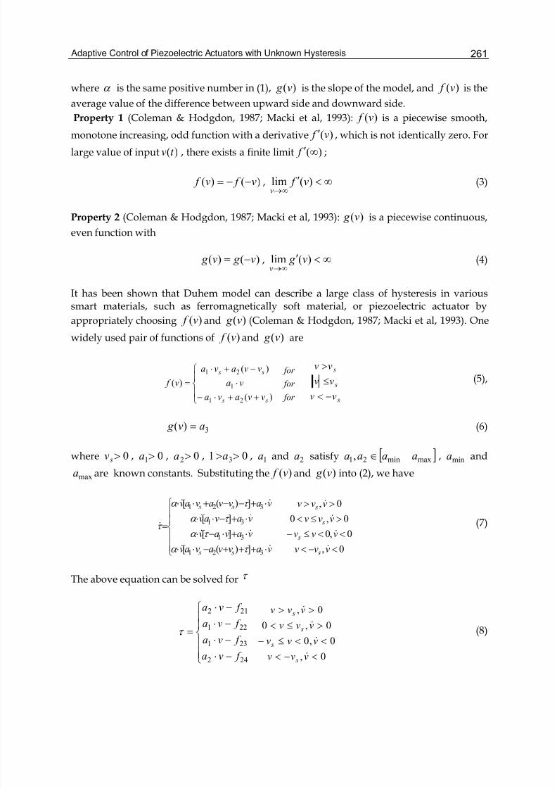
Adaptive Control of Piezoelectric Actuators with Unknown Hysteresis 261
where α is the same positive number in (1), )(v g is the slope of the model, and )(v f is the
average value of the difference between upward side and downward side.
Property 1 (Coleman & Hodgdon, 1987; Macki et al, 1993): )(v f is a piecewise smooth,
monotone increasing, odd function with a derivative )(v f ′ , which is not identically zero. For
large value of input )(t v , there exists a finite limit )(∞′ f ;
)()( v f v f −−= , ∞<′∞→
)(lim v f v
(3)
Property 2 (Coleman & Hodgdon, 1987; Macki et al, 1993): )(v g is a piecewise continuous,
even function with
)()( v g v g −= , ∞<′∞→
)(lim v g v
(4)
It has been shown that Duhem model can describe a large class of hysteresis in varioussmart materials, such as ferromagnetically soft material, or piezoelectric actuator by
appropriately choosing )(v f and )(v g (Coleman & Hodgdon, 1987; Macki et al, 1993). One
widely used pair of functions of )(v f and )(v g are
⎪⎩
⎪⎨
⎧
++⋅−
⋅
−+⋅
=
)(
)(
)(
21
1
21
s s
s s
vvava
va
vvava
v f
for
for
for
s
s
s
vv
vv
vv
−<
≤
>(5),
3)( av g = (6)
where 0> sv , 01>a , 02>a , 01 3>>a , 1a and 2a satisfy [ ]maxmin21, aaaa ∈ , mina and
maxa are known constants. Substituting the )(v f and )(v g into (2), we have
⎪⎪
⎩
⎪⎪
⎨
⎧
⋅+++−⋅⋅
⋅+⋅−⋅
⋅+−⋅⋅
⋅+−−+⋅⋅
=
vavvavav
vavav
vavav
vavvavav
s s
s s
&&
&&
&&
&&
&
321
31
31
321
])([
][
][
])([
τ α
τ α
τ α
τ α
τ
0,
0,0
0,0
0,
<−<
<<≤−
>≤<
>>
vvv
vvv
vvv
vvv
s
s
s
s
&
&
&
&
(7)
The above equation can be solved for τ
⎪⎪
⎩
⎪⎪
⎨
⎧
−⋅
−⋅
−⋅
−⋅
=
242
231
221
212
f va
f va
f va
f va
τ
0,
0,0
0,0
0,
<−<
<<≤−
>≤<
>>
vvv
vvv
vvv
vvv
s
s
s
s
&
&
&
&
(8)
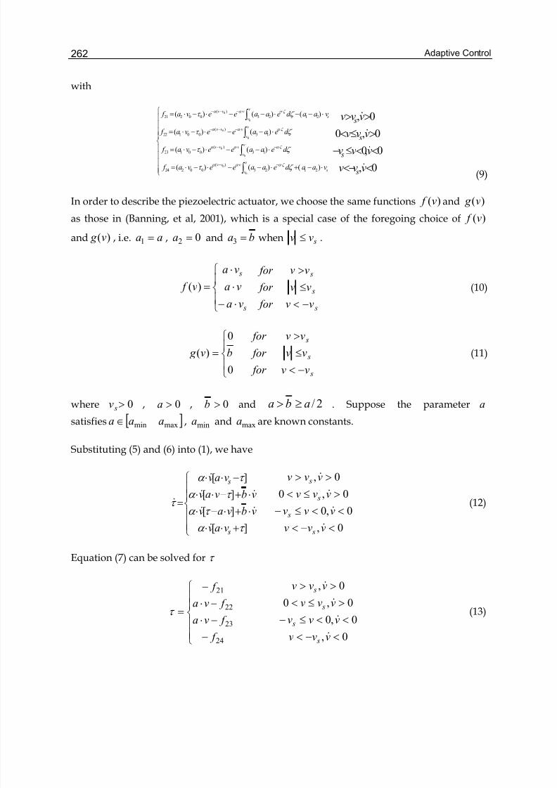
Adaptive Control262
with
0
0
0
0
0
0
0
( )
21 2 0 0 3 2 1 2
( )
22 1 0 0 3 1
( )
23 1 0 0 3 1
( )
24 2 0 0 3 2
( ) ( ) ( )
( ) ( )
( ) ( )
( ) ( ) (
vv v v
sv
vv v v
v
vv v v
v
v v v
f a v e e a a e d a a v
f a v e e a a e d
f a v e e a a e d
f a v e e a a e d a
α α α ζ
α α α ζ
α α α ζ
α α α ζ
τ ζ
τ ζ
τ ζ
τ ζ
− − − ⋅ ⋅
− − − ⋅ ⋅
− ⋅ − ⋅
− ⋅ − ⋅
= ⋅ − ⋅ − − ⋅ − − ⋅
= ⋅ − ⋅ − − ⋅
= ⋅ − ⋅ − − ⋅
= ⋅ − ⋅ − − ⋅ +
∫
∫
∫
01 2)
v
sv
a v
⎧⎪⎪⎪⎪⎨⎪⎪⎪
− ⋅⎪⎩ ∫ 0,
0,0
0,0
0,
<−<
<<≤−
>≤<
>>
vvv
vvv
vvv
vvv
s
s
s
s
&
&
&
&
(9)
In order to describe the piezoelectric actuator, we choose the same functions )(v f and )(v g
as those in (Banning, et al, 2001), which is a special case of the foregoing choice of )(v f
and )(v g , i.e. aa =1 , 02 =a and ba =3 when svv ≤ .
⎪⎩
⎪⎨
⎧
⋅−
⋅
⋅
=
s
s
va
va
va
v f )(
for
for
for
s
s
s
vv
vv
vv
−<
≤
>
(10)
⎪⎩
⎪⎨
⎧
=
0
0
)( bv g
for
for
for
s
s
s
vv
vv
vv
−<
≤
>
(11)
where 0> sv , 0>a , 0>b and 2/aba ≥> . Suppose the parameter a
satisfies [ ]maxmin aaa∈ , mina and maxa are known constants.
Substituting (5) and (6) into (1), we have
⎪⎪
⎩
⎪⎪
⎨
⎧
+⋅⋅
⋅+⋅−⋅
⋅+−⋅⋅
−⋅⋅
=
][
][
][
][
τ α
τ α
τ α
τ α
τ
s
s
vav
vbvav
vbvav
vav
&
&&
&&
&
&
0,
0,0
0,0
0,
<−<
<<≤−
>≤<
>>
vvv
vvv
vvv
vvv
s
s
s
s
&
&
&
&
(12)
Equation (7) can be solved for τ
⎪⎪
⎩
⎪⎪
⎨
⎧
−
−⋅
−⋅
−
=
24
23
22
21
f
f va
f va
f
τ
0,
0,0
0,0
0,
<−<
<<≤−
>≤<
>>
vvv
vvv
vvv
vvv
s
s
s
s
&
&
&
&
(13)
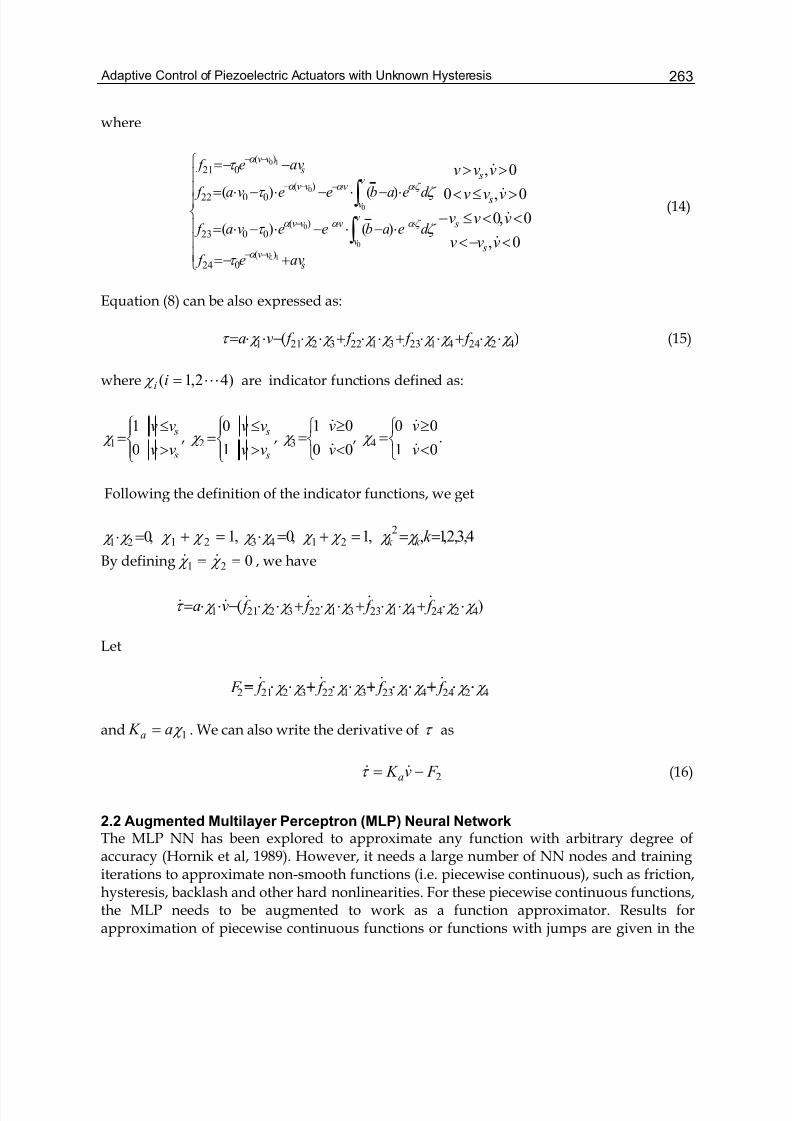
Adaptive Control of Piezoelectric Actuators with Unknown Hysteresis 263
where
⎪⎪⎪
⎩
⎪⎪⎪
⎨
⎧
+−=
⋅−⋅−⋅−⋅=
⋅−⋅−⋅−⋅=
−−=
−−
⋅−⋅−−
⋅⋅−−−
−−
∫
∫
svv
v
v
vvv
v
v
vvv
svv
ave f
d eabeeva f
d eabeeva f
ave f
10
0
0
0
0
10
)(024
)(0023
)(0022
)(021
)()(
)()(
α
ζ α α α
ζ α α α
α
τ
ζ τ
ζ τ
τ
0,
0,0
0,0
0,
<−<
<<≤−
>≤<
>>
vvv
vvv
vvv
vvv
s
s
s
s
&
&
&
&
(14)
Equation (8) can be also expressed as:
)( 42244123312232211 χ χ χ χ χ χ χ χ χ τ ⋅⋅+⋅⋅+⋅⋅+⋅⋅−⋅⋅= f f f f va (15)
where )42,1( L=ii χ are indicator functions defined as:
⎪⎩
⎪⎨⎧
>
≤=
s
s
vv
vv
0
11 χ ,
⎪⎩
⎪⎨⎧
>
≤=
s
s
vv
vv
1
02 χ ,
⎩⎨⎧
<
≥=
00
013
v
v
&
& χ ,
⎩⎨⎧
<
≥=
01
004
v
v
&
& χ .
Following the definition of the indicator functions, we get
,021 =⋅ χ χ ,121 =+ χ χ ,043 =⋅ χ χ ,121 =+ χ χ 4,3,2,1,2 == k k k χ χ
By defining 021 == χ χ && , we have
)( 42244123312232211 χ χ χ χ χ χ χ χ χ τ ⋅⋅+⋅⋅+⋅⋅+⋅⋅−⋅⋅= f f f f va &&&&&&
Let
42244123312232212 χ χ χ χ χ χ χ χ ⋅ f f f f F &&&&
and 1 χ a K a = . We can also write the derivative of τ as
2 F v K a −= &&τ (16)
2.2 Augmented Multilayer Perceptron (MLP) Neural NetworkThe MLP NN has been explored to approximate any function with arbitrary degree ofaccuracy (Hornik et al, 1989). However, it needs a large number of NN nodes and trainingiterations to approximate non-smooth functions (i.e. piecewise continuous), such as friction,hysteresis, backlash and other hard nonlinearities. For these piecewise continuous functions,the MLP needs to be augmented to work as a function approximator. Results forapproximation of piecewise continuous functions or functions with jumps are given in the
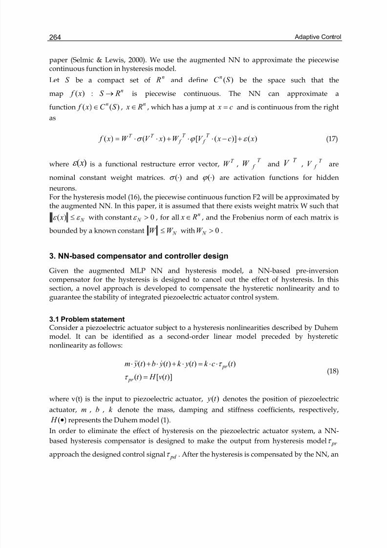
Adaptive Control264
paper (Selmic & Lewis, 2000). We use the augmented NN to approximate the piecewisecontinuous function in hysteresis model.
Let S be a compact set ofn R and define )(S C n be the space such that the
map )( x f :n
RS → is piecewise continuous. The NN can approximate a
function )()( S C x f n∈ ,
n R x∈ , which has a jump at c x = and is continuous from the right
as
)()]([)()( xc xV W xV W x f T
f T
f T T ε ϕ σ +−⋅⋅+⋅⋅= (17)
where )( xε is a functional restructure error vector, T W ,T
f W andT V ,
T f V are
nominal constant weight matrices. )(⋅σ and )(⋅ϕ are activation functions for hidden
neurons.For the hysteresis model (16), the piecewise continuous function F2 will be approximated bythe augmented NN. In this paper, it is assumed that there exists weight matrix W such that
N x ε ε ≤)( with constant 0> N ε , for alln R x∈ , and the Frobenius norm of each matrix is
bounded by a known constant N W W ≤ with 0> N W .
3. NN-based compensator and controller design
Given the augmented MLP NN and hysteresis model, a NN-based pre-inversioncompensator for the hysteresis is designed to cancel out the effect of hysteresis. In thissection, a novel approach is developed to compensate the hysteretic nonlinearity and toguarantee the stability of integrated piezoelectric actuator control system.
3.1 Problem statementConsider a piezoelectric actuator subject to a hysteresis nonlinearities described by Duhemmodel. It can be identified as a second-order linear model preceded by hystereticnonlinearity as follows:
)]([)(
)()()()(
t v H t
t ck t yk t ybt ym
pr
pr
=
⋅⋅=⋅+⋅+⋅
τ
τ &&&
(18)
where v(t) is the input to piezoelectric actuator, )(t y denotes the position of piezoelectric
actuator, m , b , k denote the mass, damping and stiffness coefficients, respectively,
)(• H represents the Duhem model (1).
In order to eliminate the effect of hysteresis on the piezoelectric actuator system, a NN-
based hysteresis compensator is designed to make the output from hysteresis model pr τ
approach the designed control signal pd τ . After the hysteresis is compensated by the NN, an
Adaptive Control of Piezoelectric Actuators with Unknown Hysteresis 265
adaptive control for piezoelectric actuator is to be designed to ensure the stability of theoverall system and the boundedness of output tracking error of the piezoelectric actuatorwith unknown hysteresis.
We consider the tracking problem, in which )(t y is to asymptotically track a reference
signal )(t yd having the properties that )(t yd and its derivatives up to second derivative are
bounded, and )(t yd && is piecewise continuous, for all 0≥t . The tracking error of the
piezoelectric actuator is defined as
)()()( t yt yt e d p −= . (19)
A filtered error is defined as
)()()( t et et r p p p p ⋅+= λ & (20)
where 0> pλ is a designed parameter.
Differentiating )(t r p and combining it with the system dynamics Eq. (18), one may obtain:
.1
))((
)(
d p pd
p pd pr p p
yc
eb
k y
ck
b
e yck
mr
ck
br
ck
m
⋅+⋅−+⋅⋅
+
⋅+⋅⋅
+−⋅⋅
−=⋅⋅
λ
λ τ
&
&&&&
(21)
The tracking error dynamics can be written as
pT
d pr p p Y r ck
br
ck
mθ τ ⋅+−⋅
⋅−=⋅
⋅& (22)
whereT
d p pd p pd d ye yeb
k yY ⎥
⎦
⎤⎢⎣
⎡⋅Λ+⋅−Λ+= &&&& )( is a regression vector
and 31 R
cck
b
ck
mT
p ∈⎥⎦
⎤⎢⎣
⎡
⋅⋅=θ is a unknown parameter vector with
3,2,1maxmin =≤≤ i p pi p θ θ θ where min pθ and max pθ are some known real numbers.
3.2 NN-based Compensator for Hysteresis
In presence of the unknown hysteresis nonlinearity, the desired control signal pd τ for the
piezoelectric actuator is different from the real control signal pr τ . Define the error as
pr pd p τ τ τ −=~ (23)
Adaptive Control266
Differentiating (23), yields
pr pd p τ τ τ &&& −=~ (24)
thus, we have
2~ F v K a pd p +−= &&& τ τ (25)
Here we utilize a second first-layer-fixed MLP to approximate the nonlinear function 2 F .
)()]([
)]([
)]([)(
223232323
22222222
21212121222
hchV W
chV W
chV W hV W F
T f
T f
T f
T f
T f
T f
T T
ε ϕ
ϕ
ϕ σ
+−⋅⋅+
−⋅⋅+
−⋅⋅⋅+⋅⋅=
(26)
where [ ]T p pd vvh 10 &τ τ = , 0 pτ is the initial value of the control signal,
T V 2 ,
T f V 21 ,
T f V 22 , and
T f V 23 are input-layer weight matrices,
T W 2 ,
T f W 21 ,
T f W 22 , and
T f W 23 are
output-layer weight matrices, 0, sv , and sv− are jump points on the output layer, and
)(⋅σ , )(21 ⋅ϕ , )(21 ⋅ϕ , and )(23 ⋅ϕ are the activation functions, and )(1 hε is the functional
restructure error in which inversion error is included. Output-layer weight
matricesT
W 2 ,T
f W 21 ,T
f W 22 andT
f W 23 are trained so that the output of NN approximates
to the nonlinear function 2 F .
LetT
sT
f sT
f T
f T
s vhV vhV hV hV vh )]()()()([),( 2323222221212 +⋅−⋅⋅⋅=Θ ϕ ϕ ϕ σ
and ][ 23222121T
f T
f T
f T T W W W W W = . The nonlinear function 2 F is expressed as:
)(),( 112 hvhW F sT ε +Θ= (27)
It is assumed that the Frobenius norm of weight matrix W1 is bounded by a known constant
N W W 11 ≤ with 01 > N W and N h 11 )( ε ε ≤ with constant 01 > N ε , for all n R x∈ .
The estimated nonlinear function 2ˆ F is constructed by using the neural network with the
weight matrix 1W :
),(ˆˆ12 sT vhW F Θ= .
Hence the restructure error between the nonlinear functions 2 F and 2ˆ F is derived as:
Adaptive Control of Piezoelectric Actuators with Unknown Hysteresis 267
)(),(~ˆ~
11222 hvhW F F F sT ε +Θ=−=
.
“where T T T W W W 111ˆ~
− .” Remark 1 When the input changes its sign derivative (Beuschel et al, 1998), the augmentedMLP can approximate the piecewise continuous functions. In the process, the “jumpfunctions” leads to vertical segments in the feed-forward pre-inversion compensation,where the “functional restructure error” can be confronted by the adaptive controller inSection III.C (Selmic & Lewis, 2000).A hysteresis pre-inversion compensator is designed:
),(ˆ~ˆ1 p s
T pd pb r vhW k v +Θ⋅++⋅⋅= τ τ μ && (28)
wherea
a
ˆˆ min=μ is an estimated constant, which satisfies 1ˆ0 ≤< with the known
boundary of [ ]maxmin aaa∈ , bk is a positive constant, a is the estimated values of a ,
and ]ˆˆˆˆ[ˆ23222121
T f
T f
T f
T T W W W W W = is the estimated output-layer weight matrix
T W 1 .
Define error matrix as:T T T
W W W 111ˆ~
−= .
Inserting (26), (28) into (25), we obtain
)(),(~~
ˆ),(ˆ
)ˆ1()ˆ1(~ˆ~
111 hvhW r K vhW
K K K k
sT
pa sT
a pd a pab p
ε μ
μ τ μ τ μ τ
+Θ⋅+⋅⋅−Θ⋅⋅
⋅−+⋅⋅−+⋅⋅⋅−= &&
(29)
We choose weight matrix update rule as
111ˆ~~),(ˆ W k vhW p p p s ⋅+⋅ΓΘ= τ τ
&(30)
where Γ is a positive adaptation gain diagonal matrix, and 1 pk is a positive constant.
Design the update rule of parameter ˆ in pre-inversion compensator v& as
]),(ˆ[~,ˆ(ˆ 1 p sT
pd p r vhW roj P +Θ+⋅⋅= τ τ η μ μ && (31)
where is positive constant, Proj(.) is a projection operator, which is defined as follows:
=Θ+⋅⋅⋅−= )],(ˆ[ˆ~,ˆ(Pr ˆ s pd pr vhoj τ μ τ η μ μ &&
Adaptive Control268
⎪⎪⎪⎪⎪⎪⎪⎪⎪
⎩
⎪⎪⎪⎪⎪⎪⎪⎪⎪
⎨
⎧
>Θ+⋅⋅⎟⎟
⎠
⎞
⎜⎜
⎝
⎛ =
≤Θ+⋅⋅⎟⎟
⎠
⎞
⎜⎜
⎝
⎛ =
≥Θ+⋅⋅=Θ+⋅⋅⋅−
<<⎟⎟
⎠
⎞
⎜⎜
⎝
⎛
<Θ+⋅⋅=
0)],(ˆ[~ˆ0
0)],(ˆ[~ˆ
0)],(ˆ[~1ˆ)],(ˆ[ˆ~
1ˆ
0)],(ˆ[~1ˆ0
2
max
min
2
max
min
2
max
min
s pd pr
s pd pr
s pd pr s pd pr
s pd pr
vhand a
aif
vhand a
aor
vhand or vh
a
aif
vhand if
τ τ η μ
τ τ η μ
τ τ η μ τ μ τ η
μ
τ τ η μ
&
&
&&
&
(32)
The adaptive NN-based pre-inversion compensator v& is developed to drive the adaptive
control signal pd τ to approach the output of hysteresis model pr τ so that the hysteretic
effect is counteracted.
3.3 Controller Design Using Estimated Hysteresis OutputIt is noticed that the output of hysteresis is not normally measurable for the plant subject tounknown hysteresis. However, considering the whole system as a dynamic model precededby Duhem model, we could design an observer to estimate the output of hysteresis based onthe input and output of the plant.
The velocity of the actuator )(t y& is assumed measurable. Define the error between the
outputs of actuator and observer as
y ye ˆ1 −= (33)
The observed output of hysteresis is denoted as pr τ and the error between the output of
hysteresis pr τ and the observed pr τ is defined as pr pr e τ τ ˆ2 −= . Then the observer is
designed as:
11ˆ e L y y += && (34)
pr pr a pr K e L F v K τ τ ˆˆˆˆ 122 −+−= && (35)
The error dynamics of the observer is obtained based on the actuator model and hysteresismodel.
11111 e Le Le −=−=&
pr pr a K e L F v K e τ ~~
1222 +−−= && (36)
where the parameter error is defined as aaa K K K ˆ~−= .
Adaptive Control of Piezoelectric Actuators with Unknown Hysteresis 269
By using the observed hysteresis output pr τ , we may define the signal error between the
adaptive control signal pd τ and the estimated hysteresis output as:
pr pd pe τ τ τ ˆ~ −= (37)
The derivative of the signal error is:
pr pr a pd pe K e L F v K τ τ τ ˆˆˆ~122 +−+−= &&& . (38)
A hysteresis pre-inversion compensator is designed:
ˆ~ˆ2 p pd peb r F k v +++⋅⋅= τ τ μ && . (39)
By substituting the neural network output ),(ˆˆ12 sT
vhW F Θ= and pre-inversion compensator
output into the derivative of the signal error, one obtains:
pr pr pa sT
a peba pd a pe K e Lr K vhW K k K K τ μ μ τ μ τ μ τ ˆˆˆ),(ˆ)ˆˆ1(~ˆˆ)ˆˆ1(~121 +−⋅−Θ−+⋅−⋅−= && (40)
The weight matrix update rule is chosen as:
111ˆ~~),(ˆ W k vhW pe p pe s ⋅+⋅ΓΘ= τ τ
&(41)
And the update rule of parameter ˆ in pre-inversion compensator v& is designed with the
same projection operator as (32):
)]),(ˆ[~,ˆ(ˆ 1 p sT
pd pe r vhW roj P +Θ+⋅⋅= τ τ η μ μ && . (42)
The update rule of parameter a K ˆ in the observer (35) is designed with the same projection
operator as (32):
)~]),(ˆ[~ˆ,ˆ(ˆ1 pe p s
T pd peaa vr vhW K roj P K τ τ τ μ γ ⋅++Θ+⋅⋅⋅= &&
& . (43)
Hence we design the adaptive controller and update rule of control parameter as:
pT
d p pd pd Y r k θ τ ˆ⋅+⋅= (44)
),ˆ(ˆˆ pd p p r Y roj P p
⋅⋅= β θ θ θ
&(45)
Adaptive Control270
where the projection operator is
0)(ˆ
0)(ˆ
0)(ˆ
ˆ
0)(ˆ
0
)(
0
),ˆ(
min
min
max
maxmin
max
ˆ
>⋅⋅=
≤⋅⋅=
≥⋅⋅=
<<
<⋅⋅=
⎪⎪⎪
⎩
⎪⎪⎪
⎨
⎧
⋅⋅
=⋅⋅
i pd p pi
i pd p pi
i pd p pi
p pi p
i pd p pi
i pd
i pd p
r Y and
r Y and
r Y and
r Y and
if
or
or
if
if
r Y
r Y roj P p
β θ θ
β θ θ
β θ θ
θ θ θ
β θ θ
β
β θ θ
With the adaptive robust controller, pre-inversion hysteresis compensator and hysteresisobserver, the overall control system of integrated piezoelectric actuator is shown in Fig. 3.The stability and convergence of the above integrated control system are summarized inTheorem 1.
Theorem 1 For a piezoelectric actuator system (18) with unknown hysteresis (1) and a
desired trajectory )(t yd , the adaptive robust controller (44), NN based compensator (39) and
hysteresis observer (34) and (35) are designed to make the output of actuator to track the
desired trajectory )(t yd . The parameters of the adaptive robust controller and the NN based
compensator are tuned by the updating rules (41)-(43) and (45). Then, the tracking error
)(t e p between the output of actuator and the desired trajectory )(t yd converge to a small
neighborhood around zero by appropriately choosing suitable control gains pd k , bk and
observer gains 21, L L and pr K .
Proof: Define a Lyapunov function
22
21
2
21
11
222
2
1
2
1)ˆ()ˆ(
2
1)ˆ(
2
1
)ˆ1(2
1)
~~(
2
1~
2
1
2
1
ee K K
K K
W W tr r ck
mV
p pT
p paa
aa
T pe p
++−⋅−⋅+−⋅
+
−⋅
+Γ⋅++⋅⋅
⋅= −
θ θ θ θ β γ
μ η
τ
The derivative of Lyapunov function is obtained:
2211
11
12
ˆ)ˆ(1
ˆ)ˆ(1
ˆ)ˆ1(1
)~ˆ(~~
eeee
K K K K W W tr r r ck
mV
pT
p p
aaaaT
pe pe p p
&&&
&&&&&&
++⋅−⋅−
−−−−Γ−⋅+⋅⋅
= −
θ θ θ β
γ μ μ
η τ τ
Introducing control strategies (39), (44) and the update rules (41)-(43), (45) into aboveequation, one obtains
22212211122
111122
2
ˆ)~
(~ˆ~
)ˆ~(~~)(~ˆˆ)(
e K e F e Le L K e Lr e
W W tr k h K k r k ck
bV
pr pr pe pr pr pe p
T pe p pe peab p pd
τ τ τ τ
τ τ ε τ μ
++−−+−−
−+⋅⋅⋅−⋅+⋅
−=&
By using 2ˆ e pr pr −= τ τ , N F 1
~ε ≤ and inequality: 22
2
1
2
1baab +≤± , one has:
Adaptive Control of Piezoelectric Actuators with Unknown Hysteresis 271
222
22
2112
211
22
22222221
22
222
111122
2
2
1)(
2
1
2
1~
2
1
2
1~
2
1~
2
1
2
1
2
1
2
1
)ˆ~(~~)(~ˆˆ)(
e K e K ee Le L
e K K e Lr e
W W tr k h K k r k ck
bV
pr pr pr N
pe pr pr pr pe pe p
T pe p pe peab p pd
−++++−
++++++++
−+⋅⋅⋅−⋅+⋅
−=
τ ε
τ τ τ τ
τ τ ε τ μ &
(46)
By using the inequality 222)(2
1baba +≤+ , we can derive the following inequality:
2221
22
21
2211111
1222
2
)2()2
3()
~(
~~
~~)12
1ˆˆ()2
1(
pr pr N pr N pe p
N pe pe pr ab p pd
K e K e L LW W W k
K K k r k ck
bV
τ ε τ
ε τ τ μ
++−−−−−⋅⋅−
⋅+⋅−−⋅⋅−⋅−+⋅
−≤&
From the Property 1 of Chapter 2 in the recent book (Ikhouane & Rodellar, 2007), we know2 pr τ is bounded (say,
22 M pr ≤τ where M is a constant), and then define a constant
2221
2221 pr pr N pr N K M K τ ε ε δ +>+= such that
δ τ
ε τ τ μ
+−−−−−⋅⋅−
⋅+⋅−−⋅⋅−⋅−+⋅
−≤
22
21
2211111
1222
2
)2()2
3()
~(
~~
~~)12
1ˆˆ()2
1(
e K e L LW W W k
K K k r k ck
bV
pr N pe p
N pe pe pr ab p pd & (47)
We select the control parameters pd k , bk and observer parameters 1 L , 2 L and pr K
satisfying the following inequalities:
02
1>−+
⋅pd k
ck
b
,
2> pr K ,
012
1ˆ 2max >−−⋅⋅ pr ab K K ak
,
221
2
3 L L >
.
Let 12
1ˆ 2max −−⋅⋅= pr abm K K ak k . If we have
m
N N p pe
k
W k 12
11 4~ ε τ
+⋅−> ,
112
111 /4/2/~
p N N N k W W W ε −+> (48)
we can easily conclude that the closed-loop system is semi-globally bounded (Su &Stepanenko, 1998).
Adaptive Control272
Hence, the following inequality holds
r m
N N pb
k
W k <
+⋅− 12
11 4 ε
where 0>r b represents the radius of a ball inside the compact set r C of the tracking error
)(~ t peτ .
Thus, any trajectory )(~ t peτ starting in compact set r r br r C ≤= converges within r C
and is bounded. Then the filtered error of system )(t r p and the tracking error of the
hysteresis )(~ t peτ converge to a small neighborhood around zero. According to the standard
Lyapunov theorem extension (Kuczmann & Ivanyi, 2002), this demonstrates the UUB
(uniformly ultimately bounded) of )(t r p , )(~ t peτ , 1
~W , 1e and 2e .
Remark 2 It is worth noting that our method is different from (Zhao & Tan, 2006; Lin et al2006) in terms of applying neural network to approximate hysteresis. The paper (Zhao &Tan, 2006) transformed multi-valued mapping of hysteresis into one-to-one mapping,whereas we sought the explicit solution to the Duhem model so that augmented MLP neuralnetworks can be used to approximate the complicated piecewise continuous unknownnonlinear functions. Viewed from a wavelet radial structure perspective, the WNN in thepaper (Lin et al 2006) can be considered as radial basis function network. In our scheme, theunknown part of the solution was approximated by an augmented MLP neural network.
4. Simulation studies
In this section, the effectiveness of the NN-based adaptive controller is demonstrated on apiezoelectric actuator described by (18) with unknown hysteresis. The coefficients of the
dynamic system and hysteresis model are m =0.016kg, b =1.2Ns/μm, k =4500N/ μm, c =0.9
μm /V, a =6, b =0.5, sv =6 μm /s, 1.0= β , 50= pd k .
The input reference signal is chosen as the desired trajectory: )2.0sin(3 t yd π ⋅= . The
control objective is to make the output signal y follow the given desired trajectory d y . From
Fig. 1, one may notice that relatively large tracking error is observed in the output responsedue to the uncompensated hysteresis.The Neural Network has 10 hidden neurons for the first part of neural network and 5
hidden neurons for the rest parts of neural network with three jumping points (0, s s vv −, ).
The gains for updating output weight matrix are all set as 252510 X diag =Γ . The activation
function )(⋅σ is a sigmoid basis function and activation function )(⋅ϕ has the
definition 01
1)( ≥⎟
⎟
⎠
⎞⎜⎜
⎝
⎛
+
−=⋅
−
−
xe
ek
x
x
α
α
ϕ , otherwise zero. The parameters for the observer are
set as: 20=a K , 100=bk , ,1.0= 1.0=γ , 10= pr K , 1001 = L , 12 = L and initial
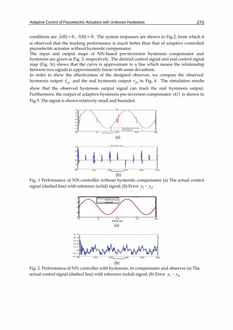
Adaptive Control of Piezoelectric Actuators with Unknown Hysteresis 273
conditions are 0)0(ˆ = y , 0)0(ˆ =τ . The system responses are shown in Fig.2, from which it
is observed that the tracking performance is much better than that of adaptive controlledpiezoelectric actuator without hysteretic compensator.The input and output maps of NN-based pre-inversion hysteresis compensator andhysteresis are given in Fig. 3, respectively. The desired control signal and real control signalmap (Fig. 3c) shows that the curve is approximate to a line which means the relationshipbetween two signals is approximately linear with some deviations.In order to show the effectiveness of the designed observer, we compare the observed
hysteresis output pr τ and the real hysteresis output pr τ in Fig. 4. The simulation results
show that the observed hysteresis output signal can track the real hysteresis output.
Furthermore, the output of adaptive hysteresis pre-inversion compensator )(t v is shown in
Fig.5. The signal is shown relatively small and bounded.
(a)
(b)Fig. 1 Performance of NN controller without hysteretic compensator (a) The actual control
signal (dashed line) with reference (solid) signal; (b) Error d y y −1
0 5 10 15 20-4
-2
0
2
4
Time (s)
Reference
Actual
(a)
(b)Fig. 2. Performance of NN controller with hysteresis, its compensator and observer (a) The
actual control signal (dashed line) with reference (solid) signal; (b) Error d y y −1
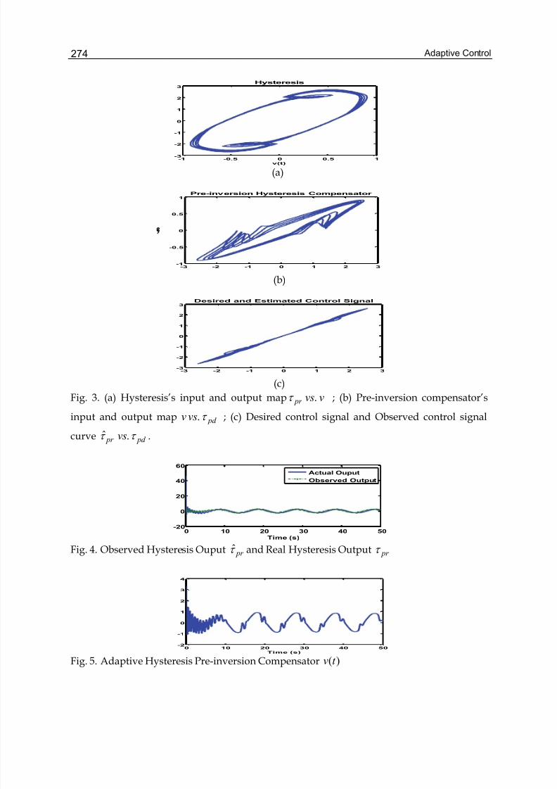
Adaptive Control274
-1 -0.5 0 0.5 1-3
-2
-1
0
1
2
3
v(t)
Hysteresis
(a)
-3 -2 -1 0 1 2 3-1
-0.5
0
0.5
1Pre-inversion Hysteresis Compensator
v ( t )
(b)
-3 -2 -1 0 1 2 3-3
-2
-1
0
1
2
3Desired and Estimated Control Signal
(c)
Fig. 3. (a) Hysteresis’s input and output map vvs pr .τ ; (b) Pre-inversion compensator’s
input and output map pd vsv τ . ; (c) Desired control signal and Observed control signal
curve pd pr vs τ τ .ˆ .
0 10 20 30 40 50-20
0
20
40
60
Time (s)
Actual Ouput
Observed Output
Fig. 4. Observed Hysteresis Ouput pr τ and Real Hysteresis Output pr τ
0 10 20 30 40 50-2
-1
0
1
2
3
4
Time (s) Fig. 5. Adaptive Hysteresis Pre-inversion Compensator )(t v
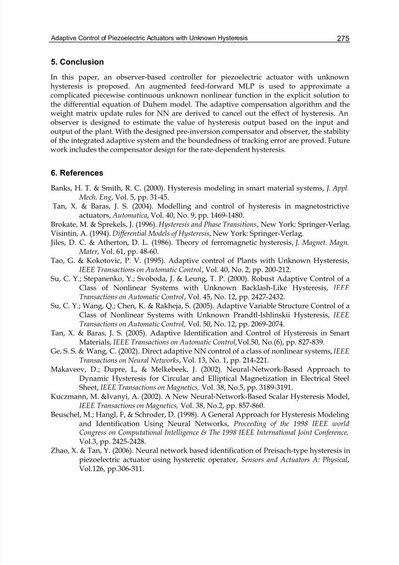
Adaptive Control of Piezoelectric Actuators with Unknown Hysteresis 275
5. Conclusion
In this paper, an observer-based controller for piezoelectric actuator with unknownhysteresis is proposed. An augmented feed-forward MLP is used to approximate acomplicated piecewise continuous unknown nonlinear function in the explicit solution tothe differential equation of Duhem model. The adaptive compensation algorithm and theweight matrix update rules for NN are derived to cancel out the effect of hysteresis. Anobserver is designed to estimate the value of hysteresis output based on the input andoutput of the plant. With the designed pre-inversion compensator and observer, the stabilityof the integrated adaptive system and the boundedness of tracking error are proved. Futurework includes the compensator design for the rate-dependent hysteresis.
6. References
Banks, H. T. & Smith, R. C. (2000). Hysteresis modeling in smart material systems, J. Appl. Mech. Eng, Vol. 5, pp. 31-45.
Tan, X. & Baras, J. S. (2004). Modelling and control of hysteresis in magnetostrictiveactuators, Automatica, Vol. 40, No. 9, pp. 1469-1480.
Brokate, M. & Sprekels, J. (1996). Hysteresis and Phase Transitions, New York: Springer-Verlag.Visintin, A. (1994). Differential Models of Hysteresis, New York: Springer-Verlag. Jiles, D. C. & Atherton, D. L. (1986). Theory of ferromagnetic hysteresis, J. Magnet. Magn.
Mater , Vol. 61, pp. 48-60.Tao, G. & Kokotovic, P. V. (1995). Adaptive control of Plants with Unknown Hysteresis,
IEEE Transactions on Automatic Control, Vol. 40, No. 2, pp. 200-212.Su, C. Y.; Stepanenko, Y.; Svoboda, J. & Leung, T. P. (2000). Robust Adaptive Control of a
Class of Nonlinear Systems with Unknown Backlash-Like Hysteresis, IEEETransactions on Automatic Control, Vol. 45, No. 12, pp. 2427-2432.
Su, C. Y.; Wang, Q.; Chen, K. & Rakheja, S. (2005). Adaptive Variable Structure Control of aClass of Nonlinear Systems with Unknown Prandtl-Ishlinskii Hysteresis, IEEETransactions on Automatic Control, Vol. 50, No. 12, pp. 2069-2074.
Tan, X. & Baras, J. S. (2005). Adaptive Identification and Control of Hysteresis in SmartMaterials, IEEE Transactions on Automatic Control,Vol.50, No.(6), pp. 827-839.
Ge, S. S. & Wang, C. (2002). Direct adaptive NN control of a class of nonlinear systems, IEEETransactions on Neural Networks, Vol. 13, No. 1, pp. 214-221.
Makaveev, D.; Dupre, L, & Melkebeek, J. (2002). Neural-Network-Based Approach toDynamic Hysteresis for Circular and Elliptical Magnetization in Electrical SteelSheet, IEEE Transactions on Magnetics, Vol. 38, No.5, pp. 3189-3191.
Kuczmann, M. &Ivanyi, A. (2002). A New Neural-Network-Based Scalar Hysteresis Model,IEEE Transactions on Magnetics, Vol. 38, No.2, pp. 857-860.
Beuschel, M.; Hangl, F, & Schroder, D. (1998). A General Approach for Hysteresis Modelingand Identification Using Neural Networks, Proceeding of the 1998 IEEE worldCongress on Computational Intelligence & The 1998 IEEE International Joint Conference, Vol.3, pp. 2425-2428.
Zhao, X. & Tan, Y. (2006). Neural network based identification of Preisach-type hysteresis inpiezoelectric actuator using hysteretic operator, Sensors and Actuators A: Physical,Vol.126, pp.306-311.
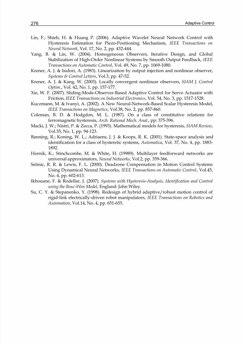
Adaptive Control276
Lin, F.; Shieh, H. & Huang P. (2006). Adaptive Wavelet Neural Network Control withHysteresis Estimation for Piezo-Positioning Mechanism, IEEE Transactions onNeural Network, Vol. 17, No. 2, pp. 432-444.
Yang, B. & Lin, W. (2004). Homogeneous Observers, Iterative Design, and GlobalStabilization of High-Order Nonlinear Systems by Smooth Output Feedback, IEEETransactions on Automatic Control, Vol. 49, No. 7, pp. 1069-1080.
Krener, A. J. & Isidori, A. (1983). Linearization by output injection and nonlinear observer,Systems & Control Letters, Vol.3, pp. 47-52.
Krener, A. J. & Kang, W. (2003). Locally convergent nonlinear observers, SIAM J. ControlOptim., Vol. 42, No. 1, pp. 157-177.
Xie, W. F. (2007). Sliding-Mode-Observer-Based Adaptive Control for Servo Actuator withFriction, IEEE Transactions on Industrial Electronics, Vol. 54, No. 3, pp. 1517-1528.
Kuczmann, M. & Ivanyi, A. (2002). A New Neural-Network-Based Scalar Hysteresis Model,IEEE Transactions on Magnetics, Vol.38, No. 2, pp. 857-860.
Coleman, B. D. & Hodgdon, M. L. (1987). On a class of constitutive relations forferromagnetic hysteresis, Arch. Rational Mech. Anal., pp: 375-396.
Macki, J. W.; Nistri, P. & Zecca, P. (1993). Mathematical models for hysteresis, SIAM Review,Vol.35, No. 1, pp. 94-123.
Banning, R.; Koning, W. L.; Adriaens, J. J. & Koops, R. K. (2001). State-space analysis andidentification for a class of hysteretic systems, Automatica, Vol. 37, No. 4, pp. 1883-1892.
Hornik, K.; Stinchcombe, M. & White, H. (19989). Multilayer feedforward networks areuniversal approximators, Neural Networks, Vol.2, pp. 359-366.
Selmic, R. R. & Lewis, F. L. (2000). Deadzone Compensation in Motion Control SystemsUsing Dynamical Neural Networks, IEEE Transactions on Automatic Control, Vol.45,No. 4, pp. 602-613.
Ikhouane, F. & Rodellar, J. (2007). Systems with Hysteresis-Analysis, Identification and Controlusing the Bouc-Wen Model, England: John Wiley.
Su, C. Y. & Stepanenko, Y. (1998). Redesign of hybrid adaptive/robust motion control ofrigid-link electrically-driven robot manipulators, IEEE Transactions on Robotics and Automation, Vol.14, No. 4, pp. 651-655.
13
On the Adaptive Tracking Control of 3-DOverhead Crane Systems
Yang, Jung Hua National Pingtung University of Science and Technology
Pingtung, Taiwan
1. Introduction
For low cost, easy assembly and less maintenance, overhead crane systems have been
widely used for material transportation in many industrial applications. Due to the
requirements of high positioning accuracy, small swing angle, short transportation time,
and high safety, both motion and stabilization control for an overhead crane system
becomes an interesting issue in the field of control technology development. Since the
overhead crane system is underactuated with respect to the sway motion, it is very difficult
to operate an overhead traveling crane automatically in a desired manner. In general,
human drivers, often assisted by automatic anti-sway system, are always involved in the
operation of overhead crane systems, and the resulting performance, in terms of swiftness
and safety, heavily depends on their experience and capability. For this reason, a growing
interest is arising about the design of automatic control systems for overhead cranes.
However, severely nonlinear dynamic properties as well as lack of actual control input for
the sway motion might bring about undesired significant sway oscillations, especially at
take-off and arrival phases. In addition, these undesirable phenomena would also make the
conventional control strategies fail to achieve the goal. Hence, the overhead crane systems
belong to the category of incomplete control system, which only allow a limited number of
inputs to control more outputs. In such a case, the uncontrollable oscillations might cause
severe stability and safety problems, and would strongly constrain the operation efficiency
as well as the application domain. Furthermore, an overhead crane system may experience
a range of parameter variations under different loading condition. Therefore, a robust and
delicate controller, which is able to diminish these unfavorable sway and uncertainties,
needs to be developed not only to enhance both efficiency and safety, but to make the
system more applicable to other engineering scopes.
The overhead crane system is non-minimum phase (or has unstable zeros in linear case) if a
nonlinear state feedback can hold the system output identically zero while the internal
dynamics become unstable. Output tracking control of non-minimum phase systems is a
highly challenging problem encountered in many practical engineering applications such as
aircraft control [1], marine vehicle control [2], flexible link manipulator control [3], inverted
pendulum system control [4]. The non-minimum phase property has long been recognized
to be a major obstacle in many control problems. It is well known that unstable zeros cannot
278 Adaptive Control
be moved with state feedback while the poles can be arbitrarily placed (if completely
controllable). In most standard adaptive control as well as in nonlinear adaptive control, all
algorithms require that the plant to be minimum phase. This chapter presents a new
procedure for designing output tracking controller for non-minimum phase systems (The
overhead crane systems).
Several researchers have dealt with the modeling and control problems of overhead crane
system. In [5], a simple proportional derivative (PD) controller is designed to asymptotically
regulate the overhead crane system to the desired position with natural damping of sway
oscillation. In [6], the authors propose an output feedback proportional derivative controller
that stabilizes a nonlinear crane system. In [7], the authors proposed an indirect adaptive
scheme, based on dynamic feedback linearization techniques, which was applied to
overhead crane systems with two control input. In [8], Li et al attacked the under-actuated
problem by blending four local controllers into one overall control strategy; moreover,
experimental results delineating the performance of the controller were also provided. In [9],
a nonlinear controller is proposed for the trolley crane systems using Lyapunov functions
and a modified version of sliding-surface control is then utilized to achieve the objective of
cart position control. However, the sway angle dynamics has not been considered for
stability analysis. In [10], the authors proposed a saturation control law based on a
guaranteed cost control method for a linearized version of 2-DOF crane system dynamics.
In [11], the authors designed a nonlinear controller for regulating the swinging energy of
the payload. In [12], a fuzzy logic control system with sliding mode Control concept is
developed for an overhead crane system. Y. Fang et al. [13] develop a nonlinear coupling
control law to stabilize a 3-DOF overhead crane system by using LaSalle invariance theorem.
However, the system parameters must be known in advance. Ishide et al. [14] train a fuzzy
neural network control architecture for an overhead traveling crane by using
back-propagation method. However, the trolley speed is still large even when the
destination is arrived, which would result in significant residual sway motion, low safety,
and poor positioning accuracy. In the paper [15], a nonlinear tracking controller for the load
position and velocity is designed with two loops: an outer loop for position tracking, and an
inner loop for stabilizing the internally oscillatory dynamics using a singular perturbation
design. But the result is available only when the sway angle dynamics is much faster than
the cart motion dynamics. In the paper [16], a simple control scheme, based on second-order
sliding modes, guarantees a fast precise load transfer and swing suppression during the
load movement, despite of model uncertainties. In the paper [17], it proposes a stabilizing
nonlinear control law for a crane system having constrained trolley stroke and pendulum
length using the Lyapunov’s second method and performs some numerical experiments to
examine the validity of the control law. In the paper [18], the variable structure control
scheme is used to regulate the trolley position and the hoisting motion towards their
desired values. However the input torques exhibit a lot of chattering. This chattering is not
desirable as it might shorten the lifetime of the motors used to drive the crane. In the paper
[19], a new fuzzy controller for anti-swing and position control of an overhead traveling
crane is proposed based on the Single Input Rule Modules (SIRMs). Computer simulation
results show that, by using the fuzzy controller, the crane can be smoothly driven to the
On the Adaptive Tracking Control of 3-D Overhead Crane Systems 279
destination in a short time with low swing angle and almost no overshoot. D. Liu et al. [20]
present a practical solution to analyze and control the overhead crane. A sliding mode fuzzy
control algorithm is designed for both X-direction and Y-direction transports of the
overhead crane. Incorporating the robustness characteristics of SMC and FLC, the proposed
control law can guarantee a swing-free transportation. J.A. Mendez et al. [21] deal with the
design and implementation of a self-tuning controller for an overhead crane. The proposed
neurocontroller is a self-tuning system consisting of a conventional controller combined
with a NN to calculate the coefficients of the controller on-line. The aim of the proposed
scheme is to reduce the training-time of the controller in order to make the real-time
application of this algorithm possible. Ho-Hoon Lee et al. [22] proposes a new approach for
the anti-swing control of overhead cranes, where a model-based control scheme is designed
based on a V-shaped Lyapunov function. The proposed control is free from the
conventional constraints of small load mass, small load swing, slow hoisting speed, and
small hoisting distance, but only guarantees asymptotic stability with all internal signals
bounded. This paper also proposes a practical trajectory generation method for a near
minimum-time control, which is independent of hoisting speed and distance. In this paper
[23], robustness of the proposed intelligent gantry crane system is evaluated. The evaluation
result showed that the intelligent gantry crane system not only has produced good
performances compared with the automatic crane system controlled by classical PID
controllers but also is more robust to parameter variation than the automatic crane system
controlled by classical PID controllers. In this paper [24], the I-PD and PD controllers
designed by using the CRA method for the trolley position and load swing angle of
overhead crane system have been proposed. The advantage of CRA method for designing
the control system so that the system performances are satisfied not only in the transient
responses but also in the steady-state responses, have also been confirmed by the simulation
results.
Although most of the control schemes mentioned above have claimed an adaptive
stabilizing tracking/regulation for the crane motion, the stability of the sway angle
dynamics is hardly taken into account. Hence, in this chapter, a nonlinear control scheme
which incorporates both the cart motion dynamics and sway angle dynamics is devised to
ensure the overall closed-loop system stability. Stability proof of the overall system is
guaranteed via Lyapunov analysis. To demonstrate the effectiveness of the proposed
control schemes, the overhead crane system is set up and satisfactory experimental results
are also given.
2. Dynamic Model of Overhead Crane
The aim of this section is to drive the dynamic model of the overhead crane system. The
model is dived using Lagrangian method. The schematic plotted in Figure 1 represents a
three degree of freedom overhead crane system. To facilitate the control development, the
following assumptions with regard to the dynamic model used to describe the motion of
overhead crane system will be made. The dynamic model for a three degree of freedom
(3-DOF) overhead crane system (see Figure 1) is assumed to have the following postulates.
A1: The payload and the gantry are connected by a mass-less, rigid link.
A2: The angular position and velocity of the payload and the rectilinear position and
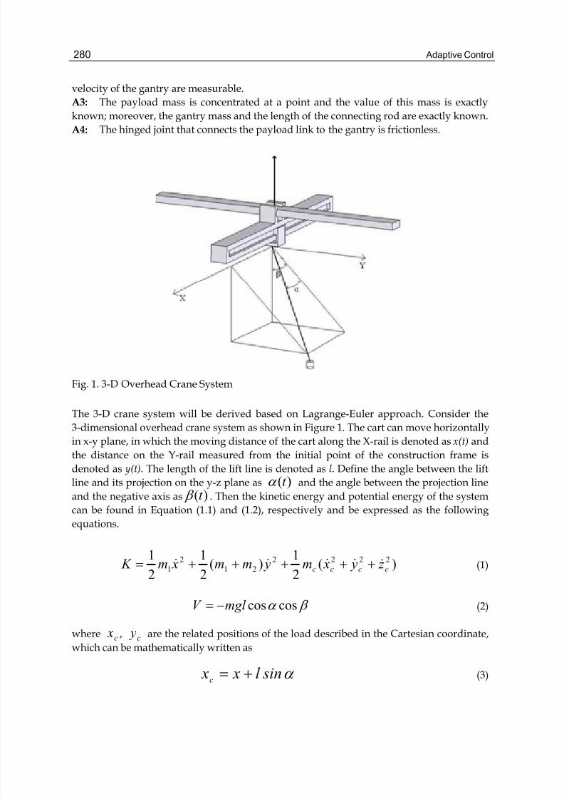
280 Adaptive Control
velocity of the gantry are measurable.
A3: The payload mass is concentrated at a point and the value of this mass is exactly
known; moreover, the gantry mass and the length of the connecting rod are exactly known.
A4: The hinged joint that connects the payload link to the gantry is frictionless.
Fig. 1. 3-D Overhead Crane System
The 3-D crane system will be derived based on Lagrange-Euler approach. Consider the
3-dimensional overhead crane system as shown in Figure 1. The cart can move horizontally
in x-y plane, in which the moving distance of the cart along the X-rail is denoted as x(t) and
the distance on the Y-rail measured from the initial point of the construction frame is
denoted as y(t). The length of the lift line is denoted as l. Define the angle between the lift
line and its projection on the y-z plane as )(t α and the angle between the projection line
and the negative axis as )(t β . Then the kinetic energy and potential energy of the system
can be found in Equation (1.1) and (1.2), respectively and be expressed as the following
equations.
)(2
1)(
2
1
2
1 2222
21
2
1 cccc z y xm ymm xm K &&&&& +++++= (1)
β α coscosmgl V −= (2)
where c x , c y are the related positions of the load described in the Cartesian coordinate,
which can be mathematically written as
α sinl x xc
+= (3)
On the Adaptive Tracking Control of 3-D Overhead Crane Systems 281
β α sincosl y yc += (4)
β α coscosl z c −= (5)
The following equations express the velocities by taking the time derivative of above
equations
α α cos&&& l x xc += (6)
β α β β α α coscossinsin &&&& l l y yc +−= (7)
β α β β α α sincoscossin &&& l l z c −−= (8)
By using the Lagrange-Euler formulation,
.4,3,2,1, ==∂
∂−⎟⎟
⎠
⎞⎜⎜⎝
⎛
∂
∂i
q
L
q
L
dt
d i
ii
τ &
(9)
where V K L −= , iq is the element of vectorT y xq ][ β α = and iτ is the
corresponding external input to the system, we have the following mathematical
representation which formulates the system motion
τ =++ )(),()( qGqqC qq M &&& (10)
where44)( ×∈ Rq M is inertia matrix of the crane system,
14),( ×∈ RqqC & is the
nonlinear terms coming from the coupling of linear and rotational motion,14)(×∈ RqG
is the terms due to gravity, andT
y x uu ]00[=τ is the input vector.
As mentioned previously, the dynamic equation of motion described the overhead crane
system also have the same properties as follows
P1: The inertia matrix )(q M is symmetric and positive definite for alln Rq∈ .
P2: There exists a matrix ),( qq B & such that qqq BqqC &&& ),(),( = , and4 R x∈∀
0)2( =− x B M xT & , i.e., 2−& is skew-symmetric. x y y x qqq Bqqq B &&&& ),(),( = .
P3: The parameters of the system can be linearly extracted as
f f qqqW qGqqC qq M Φ=++ ),,()(),()( &&&&&& (11)
where ),,( qqqW f &&& is the regressor matrix and f Φ is a vector containing the system
parameters.
Dynamic Model of Overhead Crane
In this section, an adaptive control scheme will be developed for the position tracking of an
overhead crane system.
282 Adaptive Control
2.1 Model formulation
For design convenience, a general coordinate is defined as follows
][ T T
p
T qqq θ =
where
][ y xqT
p = , ][ β α θ =T q
and using the relations in P2, the dynamic equation of an overhead crane (10) is partitioned
in the following form
⎥⎦
⎤⎢⎣
⎡=⎥
⎦
⎤⎢⎣
⎡+⎥
⎦
⎤⎢⎣
⎡⎥⎦
⎤⎢⎣
⎡+⎥
⎦
⎤⎢⎣
⎡⎥⎦
⎤⎢⎣
⎡
0)(
)( p p p
p
p pp p
T
p
p pp u
qG
qG
q
q
B B
B B
q
q
M M
M M
θ θ θθ θ
θ
θ θθ θ
θ
&
&
&&
&&
(12)
where pp M , θ p M , θθ M , pp B , θ p B , p Bθ , θθ B are 2×2 matrices partitioned from
the inertia matrix )(q M and the matrix ),( qq B & , respectively, pG , θ G are 2×1
vectors, and ][ y x
T
p uuu = . Before investigating the controller design, let the error
signals be defined as
T T T
pd eeqqe ][ θ =−= (13)
and the stable hypersurface plane is defined as
⎥⎦
⎤⎢⎣
⎡=⎥
⎦
⎤⎢⎣
⎡
+
+=+=
θ θ θ θ s
s
e K e
e K e Kee s
p p p p
&
&& (14)
where
T
y x
T
d d pd p p ee y y x xqqe ][][ ≡−−=−= ,
T T
d d d eeqqe ][][ β α θ θ θ β β α α ≡−−=−= ,
⎥⎦
⎤⎢⎣
⎡=
2
1
0
0
k
k K p , ⎥
⎦
⎤⎢⎣
⎡=
4
3
0
0
k
k K θ
and d x , d y , d α and d β are defined trajectories of x , , α and β respectively,
and p K , θ K are some arbitrary positive definite matrices.
Then, after a lot of mathematical arrangements, the dynamics of the newly defined signal
vectors p s , θ s can be derived as
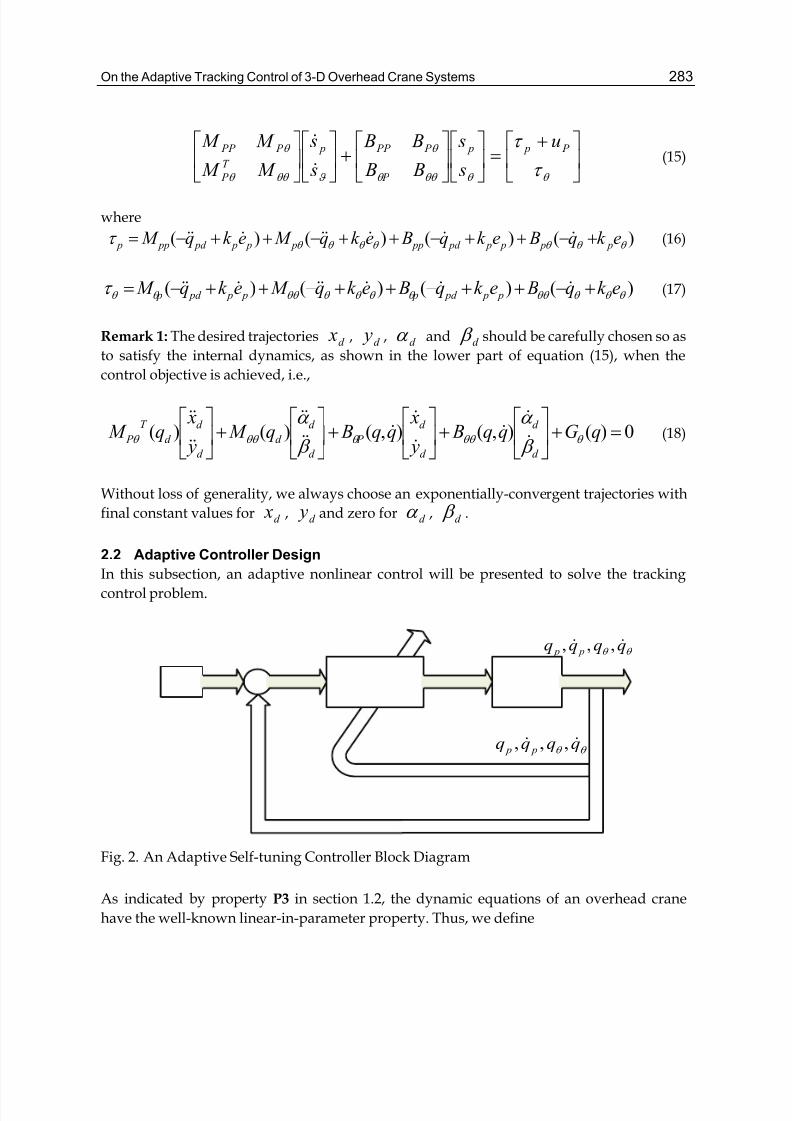
On the Adaptive Tracking Control of 3-D Overhead Crane Systems 283
⎥⎦
⎤⎢⎣
⎡ +=⎥
⎦
⎤⎢⎣
⎡⎥⎦
⎤⎢⎣
⎡+⎥
⎦
⎤⎢⎣
⎡⎥⎦
⎤⎢⎣
⎡
θ θ θθ θ
θ
ϑ θθ θ
θ
τ
τ P p p
P
P PP p
T
P
P PP u
s
s
B B
B B
s
s
M M
M M
&
&(15)
where
)()()()( θ θ θ θ θ θ θ τ ek q Bek q Bek q M ek q M p p p p pd pp p p p pd pp p +−++−++−++−= &&&&&&&& (16)
)()()()( θ θ θ θθ θ θ θ θ θθ θ θ τ ek q Bek q Bek q M ek q M p p pd p p p pd p +−++−++−++−= &&&&&&&& (17)
Remark 1: The desired trajectories d x , d y , d α and d β should be carefully chosen so as
to satisfy the internal dynamics, as shown in the lower part of equation (15), when the
control objective is achieved, i.e.,
0)(),(),()()( =+⎥⎦
⎤⎢⎣
⎡+⎥
⎦
⎤⎢⎣
⎡+⎥
⎦
⎤⎢⎣
⎡+⎥
⎦
⎤⎢⎣
⎡qGqq B
y
xqq Bq M
y
xq M
d
d
d
d
P
d
d
d
d
d
d
T
P θ θθ θ θθ θ β
α
β
α
&
&&
&
&&
&&
&&
&&
&&
(18)
Without loss of generality, we always choose an exponentially-convergent trajectories with
final constant values for d x , d y and zero for d α , d β .
2.2 Adaptive Controller Design
In this subsection, an adaptive nonlinear control will be presented to solve the tracking
control problem.
Fig. 2. An Adaptive Self-tuning Controller Block Diagram
As indicated by property P3 in section 1.2, the dynamic equations of an overhead crane
have the well-known linear-in-parameter property. Thus, we define
θ θ qqqq
p p&& ,,,
θ θ qqqq
p p&& ,,,
284 Adaptive Control
p p p p p pd ppd p p p pd pp ek Bek q Bek q M ek q M θ θ θ θ θ φ ω +++−++= )()()(11&&&&&&& (19)
θ θ θθ θ θ θ θθ θ φ ω ek Bek q Bek M ek q M p p pd p p p pd p +++++= )()()(22&&&&& (20)
where 1ω , 2ω are regressor matrices with appropriate dimensions, and 1φ , 2φ are their
corresponding vectors of unknown constant parameters, respectively. As a majority of the
adaptive controller, the following signal is defined
⎪⎩
⎪⎨
⎧
≤=
>=
>+
=
0)(,0)(,
0)(,0)(),(2
0)()),()((2
t bt Z
t bt Z t b
t Z t bt a Z
Z
x x x
x x x
x x x x
x
δ
& (21)
where xδ is some small positive constant and
)ˆ()( 222
2
θ θ θ θ φ ω ε
s K s s s
st a v
T T
p
p
x −−+
= (22)
)ˆ()( 222 θ θ θ θ φ ω ε
ε s K s s
st b v
T T
p
x −−+
= (23)
Remark 2: Note that (21) is simply to define a differential equation of which its variable
)(t Z x remains positive. Let another signal k(t) be defined to be its positive root, i.e.,
x Z k = , It can be shown that
)ˆ)(()(
1)( 222
2
θ θ θ θ φ ω ε
ε s K s s
s
sk
t k t k v
T T
p
p−−
+
+=& 0≠k (24)
In the sequel, we will first assume that there exists a measure zero set of time sequences
∞=1iit such that 0)( =it Z or 0)( =it k , ∞= ,...3,2,1i , and then, verify the existence
assumption valid.
Now let the adaptive control law be designed as
pvpv P s K u −−−= τ φ ω 11ˆ (25)
On the Adaptive Tracking Control of 3-D Overhead Crane Systems 285
⎥⎥
⎦
⎤
⎢⎢
⎣
⎡−−
+
−= )ˆ(
)1(222 θ θ θ θ φ ω
ε τ s K s s
s
sk v
T T
p
p
v (26)
where
p p p p p pd pp p p p pd pp ek Bek q Bek M ek q M θ θ θ θ φ ω ˆ)(ˆ)(ˆ)(ˆˆ11 +++++= &&&&& (27)
θ θ θθ θ θ θ θθ θ φ ω ek Bek q Bek M ek q M p p pd p p p pd pˆ)(ˆ)(ˆ)(ˆˆ
22 +++++= &&&&& (28)
and 21ˆ,ˆ φ φ are the estimates of 21,φ φ respectively, then the error dynamics can be
obtained as
⎥⎦
⎤⎢⎣
⎡
+
−=⎥
⎦
⎤⎢⎣
⎡⎥⎦
⎤⎢⎣
⎡+⎥
⎦
⎤⎢⎣
⎡⎥⎦
⎤⎢⎣
⎡+⎥
⎦
⎤⎢⎣
⎡⎥⎦
⎤⎢⎣
⎡
θ θ θ θ θ θθ θ
θ
ϑ θθ θ
θ
φ ω
τ φ ω
s K s
s
K
K
s
s
B B
B B
s
s
M M
M M
v
v p
v
vp p
P
P PP p
T
P
P PP
22
11
~
0
0
&
&
(29)
or more compactly as
⎥⎦
⎤⎢⎣
⎡
+
−=++
θ θ φ ω
τ φ ω
s K Ks sqqh sq M
v
v
22
11
~
),()( && (30)
where
⎥⎦
⎤⎢⎣
⎡
−
−=⎥
⎦
⎤⎢⎣
⎡
22
11
2
1
ˆ
ˆ~
~
φ φ
φ φ
φ
φ (31)
Moreover, let the adaptation laws be chosen as
θ ω φ
ω φ
sk
sk
b
pa
22
11
ˆ
ˆ
−=
−=
&
&
(32)
where ba k k , are some positive definite gain matrices. In what follows we will show that
the error dynamics (30) along with the adaptive laws (32) constitutes an asymptotically
stable closed-loop dynamic system. This is exactly stated in the following theorem.
286 Adaptive Control
Theorem : Consider the 3-D overhead crane system as mathematically described in (10) or (12) with
all the system parameters unknown. Then, by applying control laws (25)-(28) and adaptive laws (32),
the objective for the tracking control problem can be achieved, i.e., all signals inside the closed-loop
system (29) are bounded and 0,,, → β α eeee y x asymptotically in the sense of Lyapunov.
Proof: Define the Lyapunov function candidate as
xb
T
a
T T Z k k sq M st V 2
1~~
2
1~~
2
1)(
2
1)( 2
1
21
1
1 +++= −− φ φ φ φ
2
2
1
21
1
12
1~~
2
1~~
2
1)(
2
1k k k sq M s b
T
a
T T +++= −− φ φ φ φ
It is obvious that, due to the quadratic form of system states as well as the definition of
)(t Z x , V(t) is always positive-definite and indeed a Lyapunov function candidate. By
taking the time derivative of V we get
k k k k sq M s sq M st V b
T
a
T T T &&&&&& ++++=−−
2
1
21
1
1
~~~~)(
2
1)()( φ φ φ φ
2211
22
11 ~~)(
2
1)
~
),(( φ ω φ ω φ ω
τ φ ω θ
θ θ
T T
p
T
v
vvp
T s s sq M s s K
s K sqq B s +++⎥⎦
⎤⎢⎣
⎡
+
−−+−−= &&
)ˆ)(( 222
2
θ θ θ θ φ ω ε
ε s K s s
s
sk v
T T
p
p−−
+
++
1122222
2
11
~)ˆ)(
)1((
~φ ω φ ω φ ω
ε φ ω θ θ θ θ θ
T
p
T
v
T T
p
pT
p s s s K s s s
sk s sKs ++−−
+
−−−−=
θ θ θ θ θ θ θ θ φ ω φ ω ε
ε s K s s s K s s
s
sk v
T T
v
T T
p
p++−−
+
++ 22222
2
~)ˆ)((
Ks sT −= (33)
On the Adaptive Tracking Control of 3-D Overhead Crane Systems 287
It is clear that 0)( <t V & as long as 0> K , which then implies ∞∈ Lk s 21
~,
~,, φ φ Now,
assume that 0)( =t k instantaneously at it . Because the solution )(t Z x of the equation
(21) is well defined and is continuous for all 0≥t , k(t) is continuous at it , i.e.,
)()( +=− ii t k t k . Since V is a continuous function of k , it is clear that )(t V remains
to be continuous at it , i.e. , )()( +=− ii t V t V . Form then hypothesis, 0)( <−
it V & and
,0)( <+
it V & we hence can conclude that V is nonincreasing in t including it , which then
readily implies that ∞∈ Lk s, . Therefore, ve τ , and ∞∈ Lθ τ directly from equation
(13) and definitions of vτ and θ τ . It then follows from (30) that ∞∈ L s& . On the other
hand, if the set of time instants ∞
=1iit is measure zero, then
∞<∞−=− ∫∞ )()0(0 V V dt V & or equivalently that ∞<− ∫
∞dt s
2
0 so that 2 L s∈ .
Form the error dynamics, we can further conclusion that .∞∈ L s& Then by Barbalat’s
lemma we readily obtain that 0→ s as ∞→t asymptotically as ∞→t and therefore,
0, →ee & as ∞→t Note that in the above proof we have used the property
)),(2)(( qq Bq M && − is skew- symmetric. Finally, to complete the proof in theory, we
need to show that the above hypothesis that the set of time instants ∞=1iit is indeed
measure zero. However, it is quite straightforward to conclude the result from (21) by
simply using the fact that all signals are bounded. This completes our proof.
Remark 3: From the robustness point of view, it would be better if additional feedback term
θ sk q− is included in the control law (24). With such an inclusion, the sway stabilization
result subject to external disturbance can also be maintained as the cart arrived at its
destination. This can be easily checked from the stability proof given in the theorem.
Proof: Let the Lyapunov function candidate be chosen as
xb
T
a
T T Z k k sq M st V 2
1~~
2
1~~
2
1)(
2
1)( 2
1
21
1
1 +++= −−φ φ φ φ
2
2
1
21
1
12
1~~
2
1~~
2
1)(
2
1k k k sq M s b
T
a
T T +++= −−φ φ φ φ
and take the time derivative of V to get
k k k k sq M s sq M st V b
T
a
T T T &&&&&& ++++= −−
2
1
21
1
1
~~~~)(
2
1)()( φ φ φ φ
2211
22
11 ~~)(
2
1)
~
),(( φ ω φ ω φ ω
τ φ ω θ
θ θ
θ T T
p
T
v
qvvp
T s s sq M s s K
sk s K sqq B s +++⎥
⎦
⎤⎢⎣
⎡
+
−−−+−−= &&
288 Adaptive Control
)ˆ)(( 222
2
θ θ θ θ φ ω ε
ε s K s s
s
sk v
T T
p
p−−
+
++
pq
T s sk Ks s θ −−=
pqv
T s sk s K st V θ −−=)(&
)(2
1))(()(
2222
min θ θ λ s sk s s K t V pq pv +++−≤&
))(2
1)((
22
min θ λ s sk K pqv +−−=
Thus, the same conclusion can be made as preciously if
qv k K 2
1)(min >λ
3. Computer Simulation
In this subsection, several simulations are performed and the results also confirm the
validity of our proposed controller. The desired positions for X and Y axes are 1 m. Figure 3
shows the time response of X-direction. Figure 5 show the time responses of Y-direction. It
can be seen that the cart can simultaneously achieve the desired positions in both X and Y
axes in approximately 6 seconds with the sway angles almost converging to zero at the same
time. Figure 4 and Figure 6 show the response of the sway angle with the control scheme.
Figure 7 and Figure 8 show the velocity response of both X-direction and Y-direction. Figure
9 and Figure 10 show the control input magnitude. In Figure 11~14, the parameter estimates
are seen to converge to some constants when error tends to zero asymptotically and the time
response of the tuning function k(t) is plotted in Figure 15.
The control gains are chosen to be
⎥⎦
⎤⎢⎣
⎡=
10
05.1 pk , ⎥
⎦
⎤⎢⎣
⎡=
10
035.2θ k ,
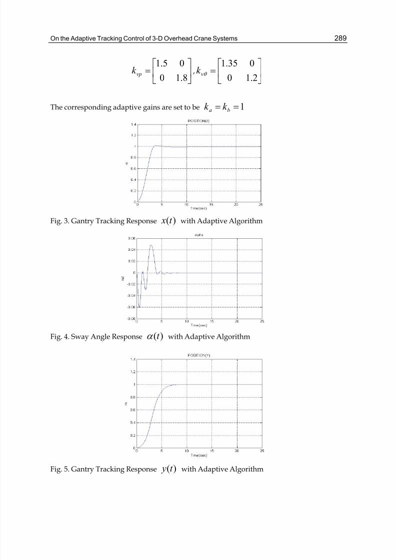
On the Adaptive Tracking Control of 3-D Overhead Crane Systems 289
⎥⎦
⎤⎢⎣
⎡=
8.10
05.1vpk , ⎥
⎦
⎤⎢⎣
⎡=
2.10
035.1θ vk
The corresponding adaptive gains are set to be 1== ba k k
Fig. 3. Gantry Tracking Response )(t x with Adaptive Algorithm
Fig. 4. Sway Angle Response )(t α with Adaptive Algorithm
Fig. 5. Gantry Tracking Response )(t y with Adaptive Algorithm
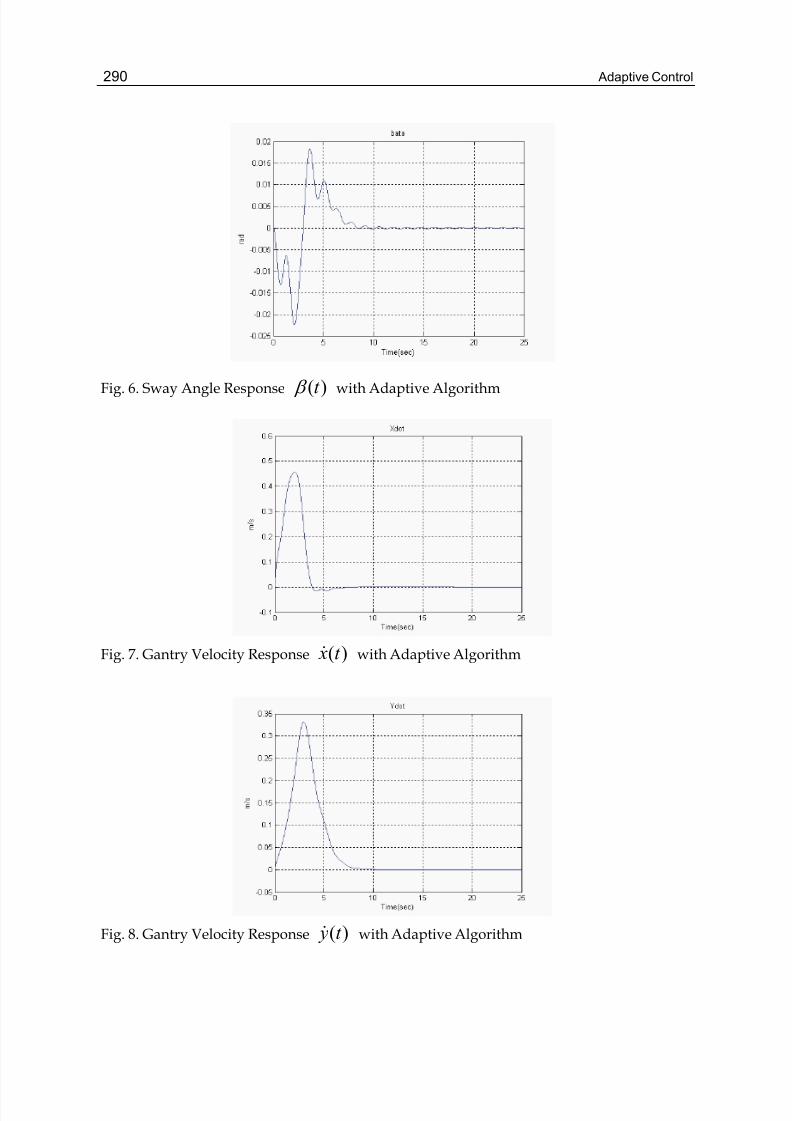
290 Adaptive Control
Fig. 6. Sway Angle Response )(t β with Adaptive Algorithm
Fig. 7. Gantry Velocity Response )(t x& with Adaptive Algorithm
Fig. 8. Gantry Velocity Response )(t y& with Adaptive Algorithm
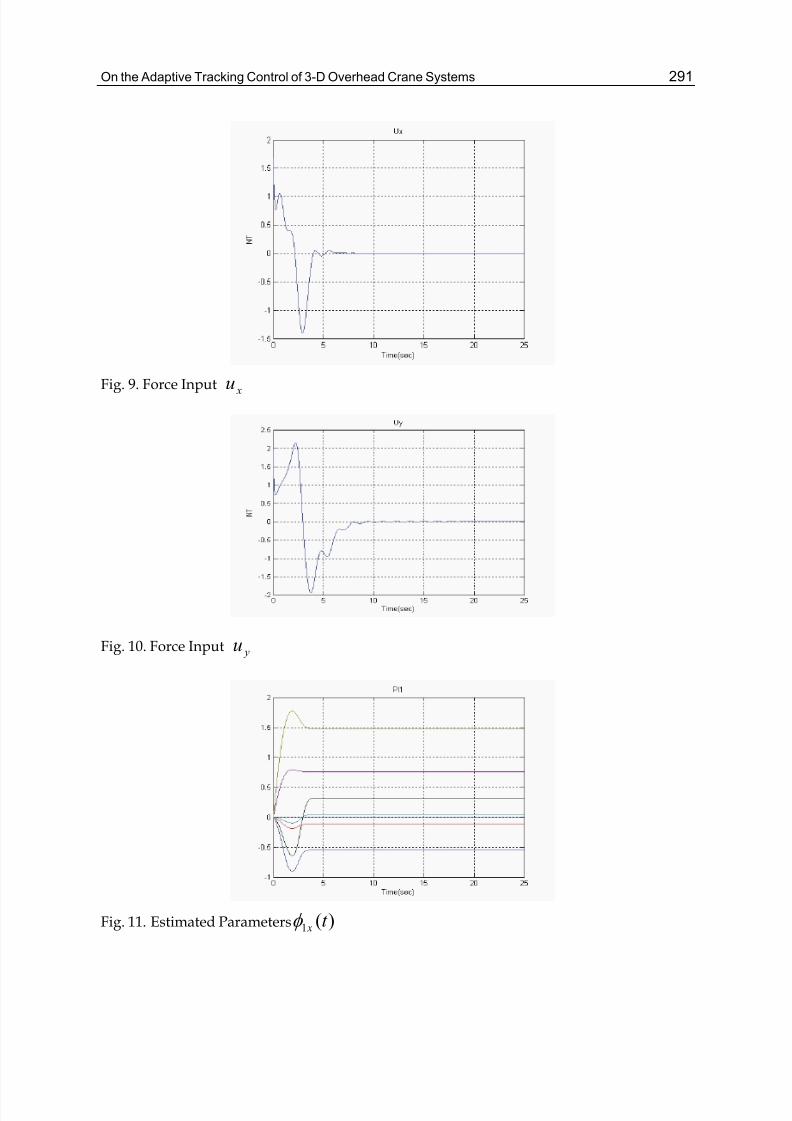
On the Adaptive Tracking Control of 3-D Overhead Crane Systems 291
Fig. 9. Force Input xu
Fig. 10. Force Input yu
Fig. 11. Estimated Parameters )(1 t xφ
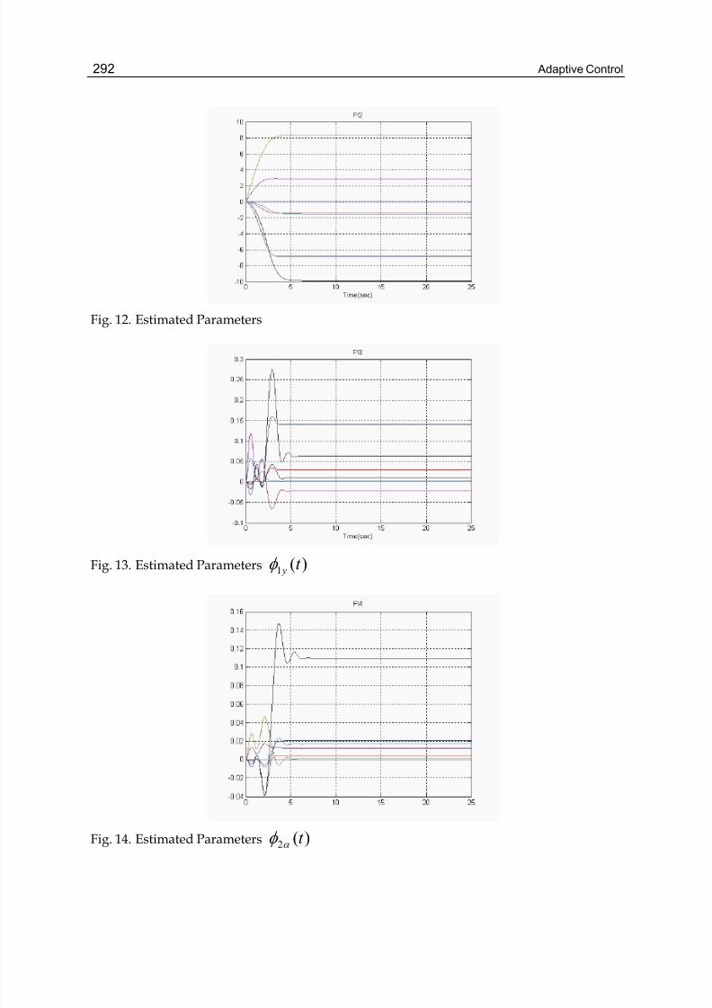
292 Adaptive Control
Fig. 12. Estimated Parameters
Fig. 13. Estimated Parameters )(1 t yφ
Fig. 14. Estimated Parameters )(2 t α φ
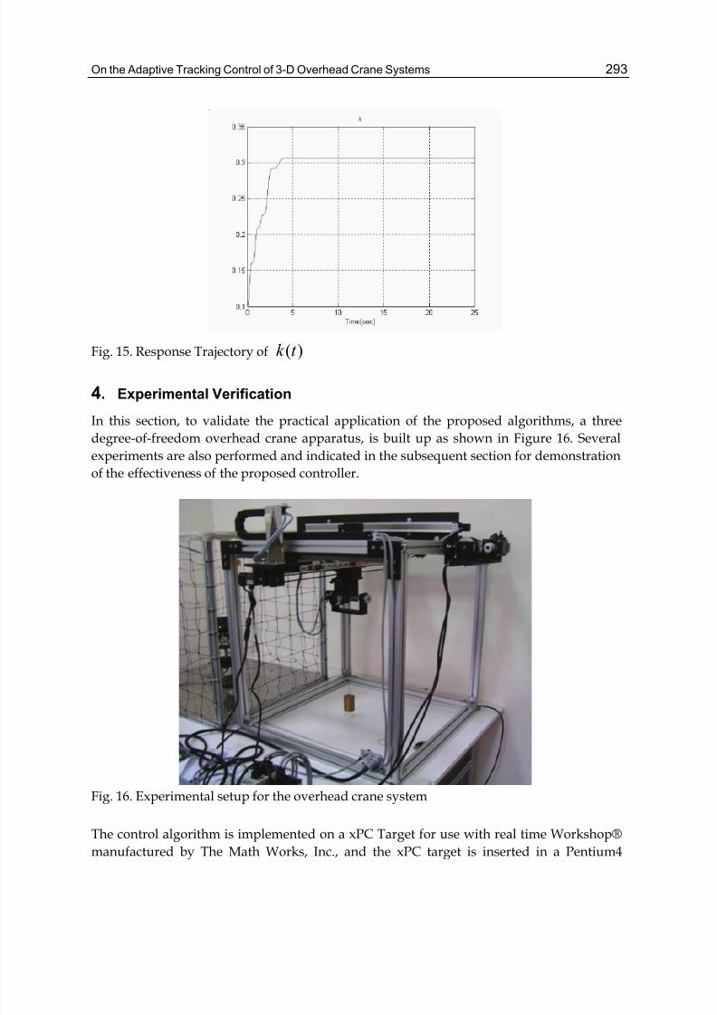
On the Adaptive Tracking Control of 3-D Overhead Crane Systems 293
Fig. 15. Response Trajectory of )(t k
4. Experimental Verification
In this section, to validate the practical application of the proposed algorithms, a three
degree-of-freedom overhead crane apparatus, is built up as shown in Figure 16. Several
experiments are also performed and indicated in the subsequent section for demonstration
of the effectiveness of the proposed controller.
Fig. 16. Experimental setup for the overhead crane system
The control algorithm is implemented on a xPC Target for use with real time Workshop®
manufactured by The Math Works, Inc., and the xPC target is inserted in a Pentium4
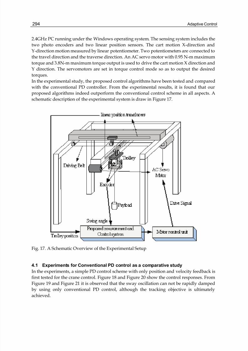
294 Adaptive Control
2.4GHz PC running under the Windows operating system. The sensing system includes the
two photo encoders and two linear position sensors. The cart motion X-direction and
Y-direction motion measured by linear potentiometer. Two potentiometers are connected to
the travel direction and the traverse direction. An AC servo motor with 0.95 N-m maximum
torque and 3.8N-m maximum torque output is used to drive the cart motion X direction and
Y direction. The servomotors are set in torque control mode so as to output the desired
torques.
In the experimental study, the proposed control algorithms have been tested and compared
with the conventional PD controller. From the experimental results, it is found that our
proposed algorithms indeed outperform the conventional control scheme in all aspects. A
schematic description of the experimental system is draw in Figure 17.
Fig. 17. A Schematic Overview of the Experimental Setup
4.1 Experiments for Conventional PD control as a comparative study
In the experiments, a simple PD control scheme with only position and velocity feedback is
first tested for the crane control. Figure 18 and Figure 20 show the control responses. From
Figure 19 and Figure 21 it is observed that the sway oscillation can not be rapidly damped
by using only conventional PD control, although the tracking objective is ultimately
achieved.
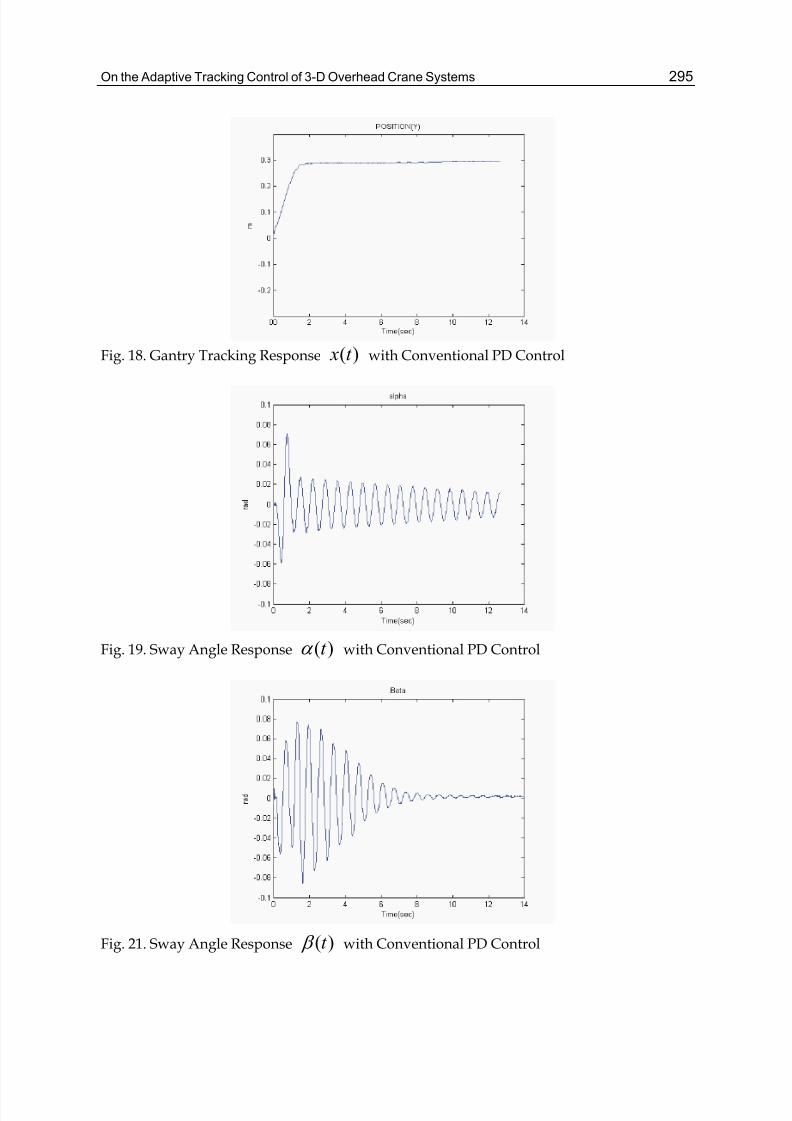
On the Adaptive Tracking Control of 3-D Overhead Crane Systems 295
Fig. 18. Gantry Tracking Response )(t x with Conventional PD Control
Fig. 19. Sway Angle Response )(t α with Conventional PD Control
Fig. 21. Sway Angle Response )(t β with Conventional PD Control
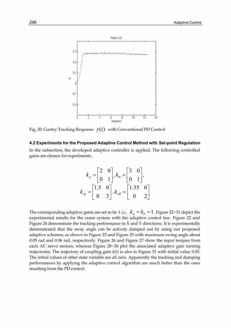
296 Adaptive Control
Fig. 20. Gantry Tracking Response )(t y with Conventional PD Control
4.2 Experiments for the Proposed Adaptive Control Method with Set-point Regulation
In the subsection, the developed adaptive controller is applied. The following controlled
gains are chosen for experiments.
⎥⎦
⎤⎢⎣
⎡=
10
02 pk , ⎥
⎦
⎤⎢⎣
⎡=
10
03θ k ,
⎥⎦
⎤⎢⎣
⎡=
30
05.1vpk , ⎥
⎦
⎤⎢⎣
⎡=
20
035.1θ vk
The corresponding adaptive gains are set to be 1 i.e., 1== ba k k . Figure 22~31 depict the
experimental results for the crane system with the adaptive control law. Figure 22 and
Figure 24 demonstrate the tracking performance in X and Y directions. It is experimentally
demonstrated that the sway angle can be actively damped out by using our proposed
adaptive schemes, as shown in Figure 23 and Figure 25 with maximum swing angle about
0.05 rad and 0.06 rad, respectively. Figure 26 and Figure 27 show the input torques from
each AC servo motors, whereas Figure 28~30 plot the associated adaptive gain turning
trajectories. The trajectory of coupling gain k(t) is also in Figure 31 with initial value 0.05.
The initial values of other state variable are all zero. Apparently the tracking and damping
performances by applying the adaptive control algorithm are much better than the ones
resulting from the PD control.
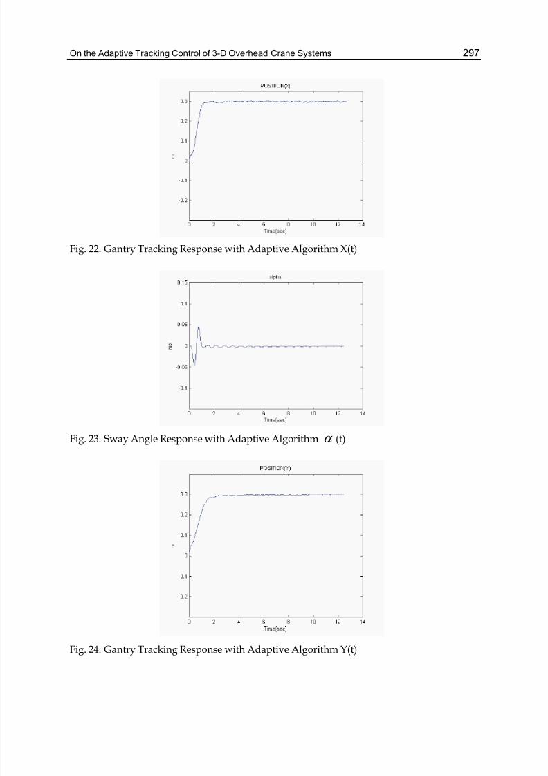
On the Adaptive Tracking Control of 3-D Overhead Crane Systems 297
Fig. 22. Gantry Tracking Response with Adaptive Algorithm X(t)
Fig. 23. Sway Angle Response with Adaptive Algorithm α (t)
Fig. 24. Gantry Tracking Response with Adaptive Algorithm Y(t)
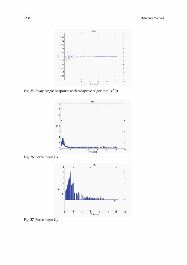
298 Adaptive Control
Fig. 25. Sway Angle Response with Adaptive Algorithm β (t)
Fig. 26. Force Input Ux
Fig. 27. Force Input Uy
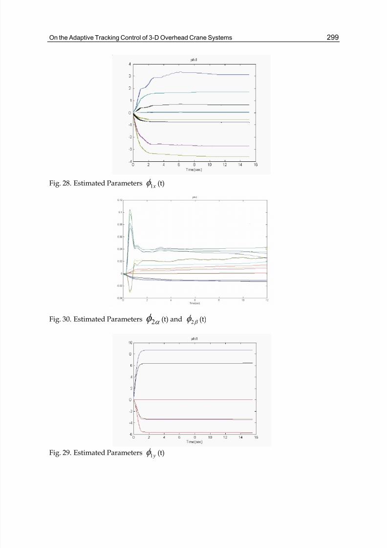
On the Adaptive Tracking Control of 3-D Overhead Crane Systems 299
Fig. 28. Estimated Parameters x1φ (t)
Fig. 30. Estimated Parameters α φ 2 (t) and β φ 2 (t)
Fig. 29. Estimated Parameters y1φ (t)
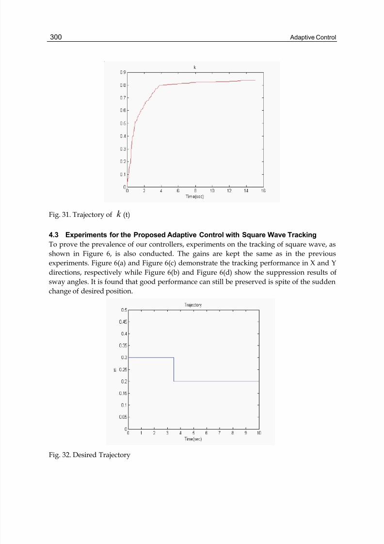
300 Adaptive Control
Fig. 31. Trajectory of k (t)
4.3 Experiments for the Proposed Adaptive Control with Square Wave Tracking
To prove the prevalence of our controllers, experiments on the tracking of square wave, as
shown in Figure 6, is also conducted. The gains are kept the same as in the previous
experiments. Figure 6(a) and Figure 6(c) demonstrate the tracking performance in X and Y
directions, respectively while Figure 6(b) and Figure 6(d) show the suppression results of
sway angles. It is found that good performance can still be preserved is spite of the sudden
change of desired position.
Fig. 32. Desired Trajectory
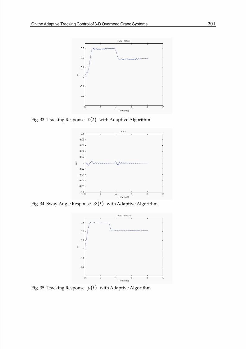
On the Adaptive Tracking Control of 3-D Overhead Crane Systems 301
Fig. 33. Tracking Response )(t x with Adaptive Algorithm
Fig. 34. Sway Angle Response )(t α with Adaptive Algorithm
Fig. 35. Tracking Response )(t y with Adaptive Algorithm
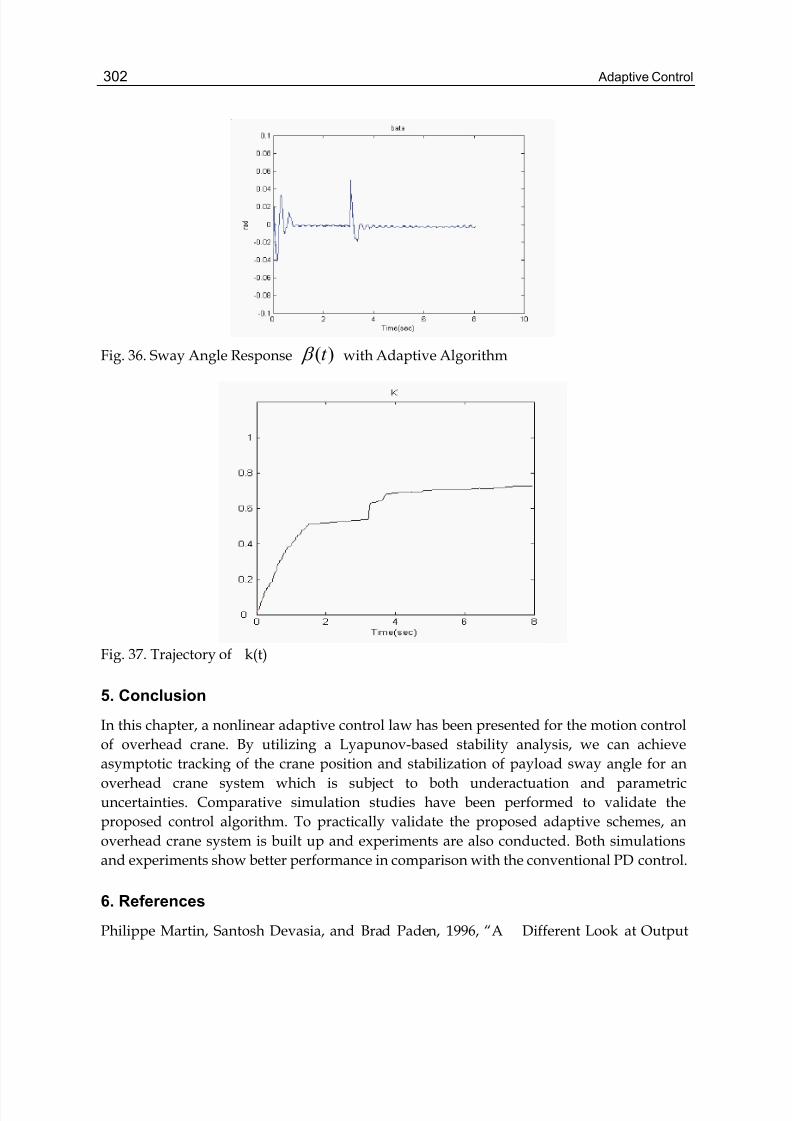
302 Adaptive Control
Fig. 36. Sway Angle Response )(t β with Adaptive Algorithm
Fig. 37. Trajectory of k(t)
5. Conclusion
In this chapter, a nonlinear adaptive control law has been presented for the motion control
of overhead crane. By utilizing a Lyapunov-based stability analysis, we can achieve
asymptotic tracking of the crane position and stabilization of payload sway angle for an
overhead crane system which is subject to both underactuation and parametric
uncertainties. Comparative simulation studies have been performed to validate the
proposed control algorithm. To practically validate the proposed adaptive schemes, an
overhead crane system is built up and experiments are also conducted. Both simulations
and experiments show better performance in comparison with the conventional PD control.
6. References
Philippe Martin, Santosh Devasia, and Brad Paden, 1996, “A Different Look at Output
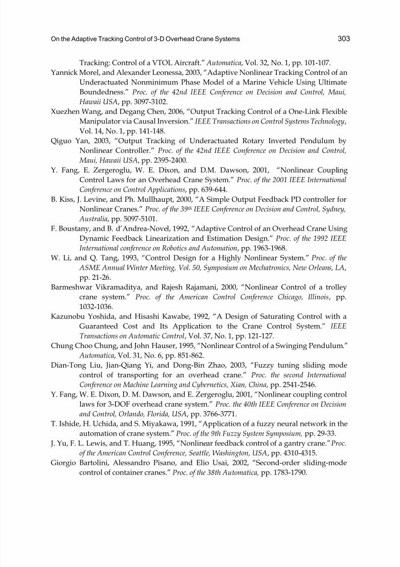
On the Adaptive Tracking Control of 3-D Overhead Crane Systems 303
Tracking: Control of a VTOL Aircraft.” Automatica, Vol. 32, No. 1, pp. 101-107.
Yannick Morel, and Alexander Leonessa, 2003, “Adaptive Nonlinear Tracking Control of an
Underactuated Nonminimum Phase Model of a Marine Vehicle Using Ultimate
Boundedness.” Proc. of the 42nd IEEE Conference on Decision and Control, Maui,
Hawaii USA, pp. 3097-3102.
Xuezhen Wang, and Degang Chen, 2006, “Output Tracking Control of a One-Link Flexible
Manipulator via Causal Inversion.” IEEE Transactions on Control Systems Technology,
Vol. 14, No. 1, pp. 141-148.
Qiguo Yan, 2003, “Output Tracking of Underactuated Rotary Inverted Pendulum by
Nonlinear Controller.” Proc. of the 42nd IEEE Conference on Decision and Control,
Maui, Hawaii USA, pp. 2395-2400.
Y. Fang, E. Zergeroglu, W. E. Dixon, and D.M. Dawson, 2001, “Nonlinear Coupling
Control Laws for an Overhead Crane System.” Proc. of the 2001 IEEE International
Conference on Control Applications, pp. 639-644.
B. Kiss, J. Levine, and Ph. Mullhaupt, 2000, “A Simple Output Feedback PD controller for
Nonlinear Cranes.” Proc. of the 39th IEEE Conference on Decision and Control, Sydney,
Australia, pp. 5097-5101.
F. Boustany, and B. d’Andrea-Novel, 1992, “Adaptive Control of an Overhead Crane Using
Dynamic Feedback Linearization and Estimation Design.” Proc. of the 1992 IEEE
International conference on Robotics and Automation, pp. 1963-1968.
W. Li, and Q. Tang, 1993, “Control Design for a Highly Nonlinear System.” Proc. of the
ASME Annual Winter Meeting, Vol. 50, Symposium on Mechatronics, New Orleans, LA,
pp. 21-26.
Barmeshwar Vikramaditya, and Rajesh Rajamani, 2000, “Nonlinear Control of a trolley
crane system.” Proc. of the American Control Conference Chicago, Illinois, pp.
1032-1036.
Kazunobu Yoshida, and Hisashi Kawabe, 1992, “A Design of Saturating Control with a
Guaranteed Cost and Its Application to the Crane Control System.” IEEE
Transactions on Automatic Control, Vol. 37, No. 1, pp. 121-127.
Chung Choo Chung, and John Hauser, 1995, “Nonlinear Control of a Swinging Pendulum.”
Automatica, Vol. 31, No. 6, pp. 851-862.
Dian-Tong Liu, Jian-Qiang Yi, and Dong-Bin Zhao, 2003, “Fuzzy tuning sliding mode
control of transporting for an overhead crane.” Proc. the second International
Conference on Machine Learning and Cybernetics, Xian, China, pp. 2541-2546.
Y. Fang, W. E. Dixon, D. M. Dawson, and E. Zergeroglu, 2001, “Nonlinear coupling control
laws for 3-DOF overhead crane system.” Proc. the 40th IEEE Conference on Decision
and Control, Orlando, Florida, USA, pp. 3766-3771.
T. Ishide, H. Uchida, and S. Miyakawa, 1991, “Application of a fuzzy neural network in the
automation of crane system.” Proc. of the 9th Fuzzy System Symposium, pp. 29-33.
J. Yu, F. L. Lewis, and T. Huang, 1995, “Nonlinear feedback control of a gantry crane.”Proc.
of the American Control Conference, Seattle, Washington, USA, pp. 4310-4315.
Giorgio Bartolini, Alessandro Pisano, and Elio Usai, 2002, “Second-order sliding-mode
control of container cranes.” Proc. of the 38th Automatica, pp. 1783-1790.
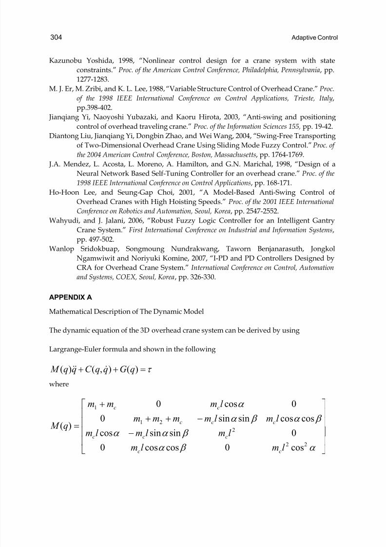
304 Adaptive Control
Kazunobu Yoshida, 1998, “Nonlinear control design for a crane system with state
constraints.” Proc. of the American Control Conference, Philadelphia, Pennsylvania, pp.
1277-1283.
M. J. Er, M. Zribi, and K. L. Lee, 1988, “Variable Structure Control of Overhead Crane.” Proc.
of the 1998 IEEE International Conference on Control Applications, Trieste, Italy,
pp.398-402.
Jianqiang Yi, Naoyoshi Yubazaki, and Kaoru Hirota, 2003, “Anti-swing and positioning
control of overhead traveling crane.” Proc. of the Information Sciences 155, pp. 19-42.
Diantong Liu, Jianqiang Yi, Dongbin Zhao, and Wei Wang, 2004, “Swing-Free Transporting
of Two-Dimensional Overhead Crane Using Sliding Mode Fuzzy Control.” Proc. of
the 2004 American Control Conference, Boston, Massachusetts, pp. 1764-1769.
J.A. Mendez, L. Acosta, L. Moreno, A. Hamilton, and G.N. Marichal, 1998, “Design of a
Neural Network Based Self-Tuning Controller for an overhead crane.” Proc. of the
1998 IEEE International Conference on Control Applications, pp. 168-171.
Ho-Hoon Lee, and Seung-Gap Choi, 2001, “A Model-Based Anti-Swing Control of
Overhead Cranes with High Hoisting Speeds.” Proc. of the 2001 IEEE International
Conference on Robotics and Automation, Seoul, Korea, pp. 2547-2552.
Wahyudi, and J. Jalani, 2006, “Robust Fuzzy Logic Controller for an Intelligent Gantry
Crane System.” First International Conference on Industrial and Information Systems,
pp. 497-502.
Wanlop Sridokbuap, Songmoung Nundrakwang, Taworn Benjanarasuth, Jongkol
Ngamwiwit and Noriyuki Komine, 2007, “I-PD and PD Controllers Designed by
CRA for Overhead Crane System.” International Conference on Control, Automation
and Systems, COEX, Seoul, Korea, pp. 326-330.
APPENDIX A
Mathematical Description of The Dynamic Model
The dynamic equation of the 3D overhead crane system can be derived by using
Largrange-Euler formula and shown in the following
τ =++ )(),()( qGqqC qq M &&&
where
⎥⎥⎥⎥
⎦
⎤
⎢⎢⎢⎢
⎣
⎡
−
−++
+
=
α β α
β α α
β α β α
α
22
2
21
1
cos0coscos0
0sinsincos
coscossinsin0
0cos0
)(
l ml m
l ml ml m
l ml mmmm
l mmm
q M
cc
ccc
ccc
cc
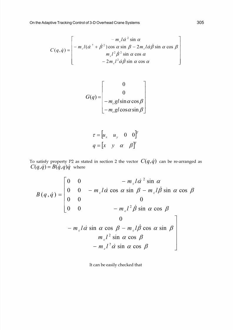
On the Adaptive Tracking Control of 3-D Overhead Crane Systems 305
⎥⎥⎥⎥⎥
⎦
⎤
⎢⎢⎢⎢⎢
⎣
⎡
−
−+−
−
=
α α β α
α α β
β α β α β α β α
α α
cossin2
cossin
cossin2sincos)(
sin
),(
2
22
22
2
&&
&
&&&&
&
&
l m
l m
l ml m
l m
qqC
c
c
cc
c
⎥⎥⎥⎥
⎦
⎤
⎢⎢⎢⎢
⎣
⎡
−
−=
β α
β α
sincos
cossin
0
0
)(
gl m
gl mqG
c
c
[ ]
[ ]T
T
y x
y xq
uu
β α
τ
=
= 00
To satisfy property P2 as stated in section 2 the vector ),( qqC & can be re-arranged as
qqq BqqC &&& ),(),( = where
⎥⎥⎥⎥
⎦
⎤
−
−−
⎢⎢⎢⎢⎢
⎣
⎡
−
−−
−
=
β α α
β α
β α β β α α
β α β
β α β β α α
α α
cossin
cossin
sincoscossin
0
cossin00
000
cossinsincos00
sin00
),(
2
2
2
2
&
&&
&
&&
&
&
l m
l m
l ml m
l m
l ml m
l m
qq B
c
c
cc
c
cc
c
It can be easily checked that
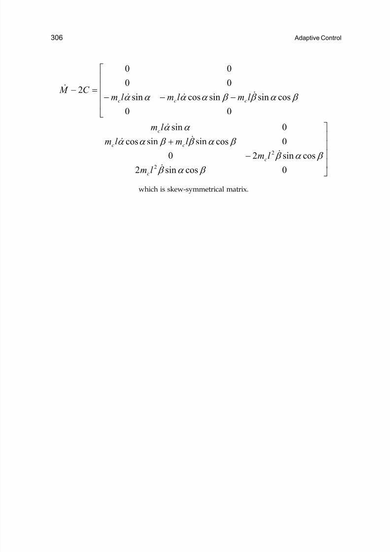
306 Adaptive Control
⎥⎥⎥⎥
⎦
⎤
−
+
⎢⎢⎢⎢
⎣
⎡
−−−=−
0cossin2
cossin20
0cossinsincos
0sin
00
cossinsincossin
00
00
2
2
2
β α β
β α β
β α β β α α
α α
β α β β α α α α
&
&
&&
&
&&&
&
l m
l m
l ml m
l m
l ml ml mC M
c
c
cc
c
ccc
which is skew-symmetrical matrix.
14
Adaptive Inverse Optimal Control of a Magnetic Levitation System
Yasuyuki Satoh1, Hisakazu Nakamura1,Hitoshi Katayama2 and Hirokazu Nishitani1
1Nara Institute of Science and Technology, 2Shizuoka University Japan
1. Introduction
In recent years, control Lyapunov functions (CLFs) and CLF-based control designs haveattracted much attention in nonlinear control theory. Particularly, CLF-based inverseoptimal controllers are some of the most effective controllers for nonlinear systems [Sontag(1989); Freeman & Kokotović (1996); Sepulchre et al. (1997); Li & Krstić (1997); Krstić & Li(1998)]. These controllers minimize a meaningful cost function and guarantee the optimalityand a stability margin. Moreover, we can obtain the optimal controller without solving theHamilton-Jacobi equation. An inverse optimal controller with input constraints has alsobeen proposed [Nakamura et al. (2007)]. On the other hand, these controllers assume thatthe desired state of the controlled system is an equilibrium state. Then, if the controlledsystem does not satisfy the assumption, we have to use a pre-feedback control designmethod to the assumption is virtually satisfied. However, a pre-feedback control designcauses the luck of robustness. This implies that a stability margin of inverse optimalcontrollers is lost. Hence the designed controller does not asymptotically stabilize thesystem if there exists a parameter uncertainty in the system.In this article, we study how to guarantee a stability margin when the pre-feedbackcontroller design is used. We consider a magnetic levitation system as an actual controlexample and propose an adaptive inverse optimal controller which guarantees a gainmargin for the system. The proposed controller consists of a conventional inverse optimalcontroller and a pre-feedback compensator with an adaptive control mechanism. Byintroducing adaptive control law based on adaptive control Lyapunov functions (ACLFs),we can successfully guarantee the gain margin for the closed loop system. Furthermore, weapply the proposed method to the actual magnetic levitation system and confirm itseffectiveness by experiments.This article is organized as follows. Section 2 introduces some mathematical notation anddefinitions, and outlines the previous results of CLF-based inverse optimal control design.Section 3 describes the experimental setup of the magnetic levitation system and itsmathematical model. In section 4, we design an inverse optimal controller with a pre-feedback compensator for the magnetic levitation system. The problem with the designedcontroller is demonstrated by the experiment in section 5. To deal with the problem, we
Adaptive Control308
propose an adaptive inverse optimal controller in section 6. The effectiveness of theproposed controller is confirmed by the experiment in section 7. Section 8 is devoted toconcluding remarks.
2. Preliminaries
In this section, we introduce some mathematical definitions and preliminary results of CLF-based inverse optimal control. We also refer to ACLF-based adaptive control techniques.
2.1 Mathematical notations and definitionsWe use the notation ),0[:0 ∞=≥ R .
Definition 1 A function )sgn( y is defined for R y∈ by the following equation:
⎪⎩
⎪⎨
⎧
>
=
<−
=
).0(1
)0(0
)0(1
)sgn(
y
y
y
y
(1)
In this section, we consider the following input affine nonlinear system:
,)()( u xg x f x +=& (2)
where n R x∈ is a state vector, m RU u ⊆∈ is an input vector and U is a convex subspace
containing the origin 0=u . We assume that nn R R f →: and mnn R Rg ×→: are continuous
vector fields, and 0)0( = f . Let V L f and V Lg
be the Lie derivative of )( x f and )( xg
respectively, which are defined by
),()( x f x
V xV L f ∂
∂=
(3)
).()( xg x
V xV Lg ∂
∂=
(4)
For simplicity of notations, we shall drop )( x in the remaining of this article. We suppose
that a local control Lyapunov function is given for system (2).
Definition 2 A smooth proper positive-definite function0: ≥→ R X V defined on a
neighborhood of the origin n R X ⊂ is said to be a local control Lyapunov function (localCLF) for system (2) if the condition
0inf <⋅+⊂
uV LV L g f U u
(5)
Adaptive Inverse Optimal Control of a Magnetic Levitation System 309
is satisfied for all 0\ X x∈ . Moreover, )( xV is said to be a control Lyapunov function
(CLF) for system (2) if )( xV is a function defined on entire n R and condition (3) is satisfied
for all 0\n R x∈ .
If there exists no input constraint ( m RU = ), a smooth proper positive-definite function
0: ≥→ R RV n is a CLF if and only if
.0,00 ≠∀<⇒= xV LV L f g (6)
In this article, we guarantee the robustness of controllers by sector margins and gainmargins.
Definition 3 A locally Lipschitz continuous mapping m Ru ∈)(φ is said to be a sector
nonlinearity in ),( β α with respect to m Ru∈ if the following conditions are satisfied:
,0,)( ≠∀<< uuuuuuu T T T β φ α
.0)0( =φ (7)
Definition 4 System (2) is said to have a sector margin ),( β α with respect to m Ru∈ if the
closed system
)()()( u xg x f x φ +=& (8)
is asymptotically stable, where )(uφ is any sector nonlinearity in ),( β α with respect tom Ru∈ .
Definition 5 System (2) is said to have a gain margin ),( β α with respect to m Ru∈ if the
closed system (8) is asymptotically stable, when )(uφ is given as follows:
).,(,)( β α κ κ φ ∈= uu (9)
By the definition, gain margins are the special case of sector margins. If system (2) has asector margin ),( β α , it also has a gain margin ),( β α .
2.2 Inverse optimal controller We introduce the inverse optimal controller proposed by Nakamura et al [Nakamura et al.(2007)]. The following results are obtained for system (2) with input constraint
,)(:
1
1 ⎪⎭
⎪⎬
⎫
⎪⎩
⎪⎨
⎧
<⎟ ⎠
⎞⎜⎝
⎛ =∈= ∑
=
xC uu RuU k m
i
k
ik
mC
k
(10)
Adaptive Control310
where ∞<< k 1 is a constant and 0)( > xC is continuous on n R .
Theorem 1 We consider system (2) with input constraint (10). Let )( xV be a local CLF for
system (2) and 01 >a be the maximum number satisfying
,0inf <⋅+∈
uV LV L g f U u
C k
.)(|: 11 a xV xW x <=∈∀ (11)
Then,1W is a domain in which the origin is asymptotically stabilizable. If )( xV is a CLF,
then ∞=1a and n RW =1.
Theorem 2 We consider system (2) with input constraint (10) . Let )( xV be a local CLF for
system (2) , )( xP be a function defined by
,)(
)(
1−
=
k
k g
f
V L xC
V L xP
(12)
and ),0( 1aar ∈ be the maximum number such that the condition
,01
inf <⎭⎬⎫
⎩⎨⎧
⋅−
+∈
uV Lk
k V L g f
U u C k
r r a xV xW x <=∈∀ )(|: (13)
is satisfied, and d be a positive constant. Then, input
)sgn()(
11
1
V LV L x R
uii g
k gi
−−= ),,,1( mi K= (14)
⎪⎪⎪
⎩
⎪⎪⎪
⎨
⎧
=
≠
++−
+
= −
−
−
−
−
−
),0()(
2
)0(
)()(1
))(2(
)( 1
1
1
1
1
1
1
1
1
V L xq
V L
V L xqPPk
k
V LV L xq
x R
g
g
k
k
k g
k
k
k gk
k
k g
.
(15)
)()( 1
1
xdC xq k −= (16)
Adaptive Inverse Optimal Control of a Magnetic Levitation System 311
asymptotically stabilizes the origin inr W , and minimizes the cost function:
,)(
)(0
1
∫∞ −
⎭⎬⎫
⎩⎨⎧
+= dt uk
x R xl J
k
k
k
.)(
11)( 1
1
V LV L x Rk
k xl f
k
k
k
k g−⋅
−= −
−
(17)
Moreover, it achieves at least a sector margin ),( β α inr W .
2.3 Adaptive control problemWe consider an adaptive control problem for nonlinear systems. In this section, weintroduce some definitions and properties. We consider the following input affine nonlinearsystem:
,)()()( 10 u xg x f x f x ++= θ & (18)
where n R x∈ is a state vector, m Ru∈ is an input vector, and p R∈θ is a constant unknown
parameter vector. We assume that nn R R f →:0, mnn
R Rg×→: and pnn
R R f ×→:1
are
continuous vector fields, and 0)0(0 = f . Note that there exists no input constraint.
The stabilizability of the system with unknown parameters is defined as the following.
Definition 6 Let θ be an estimate of θ . We say that (18) is globally adaptively stabilizable
if there exist a function )ˆ,( θ α x continuous on pn R R ×0\ with 0)ˆ,0( ≡θ α , a continuous
function )ˆ,( θ τ x , and a positive definite symmetric p p × matrix Γ , such that the dynamic
controller
),ˆ,( θ α xu = (19)
)ˆ,(ˆ θ τ θ xΓ=& (20)
guarantees that the solution )ˆ,( θ x is globally bounded, and 0→ x as ∞→t for any value
of the unknown parameter p R∈θ .
For the stabilization problem, we introduce an adaptive control Lyapunov function (ACLF)as the following.
Definition 7 We consider system (18) and assume that ),( θ xV a is a CLF for system (18).
Then, ),( θ xV a is called an adaptive control Lyapunov function (ACLF) for system (18) if
there exists a positive-definite symmetric matrix Γ such that for each p R∈θ ,
aV is a CLF
for the modified system
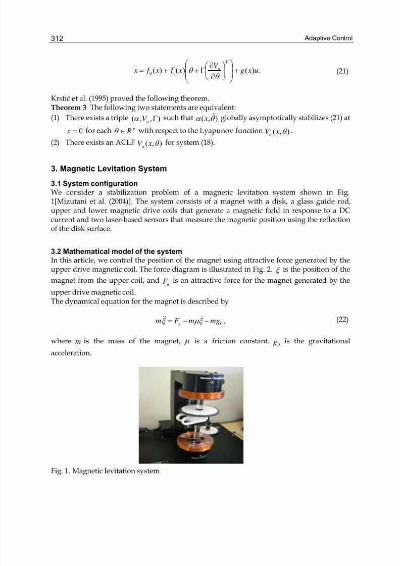
Adaptive Control312
.)()()( 10 u xgV
x f x f x
T
a +⎟⎟
⎠
⎞
⎜⎜
⎝
⎛ ⎟ ⎠
⎞⎜⎝
⎛ ∂
∂Γ++=
θ θ & (21)
Krstić et al. (1995) proved the following theorem.Theorem 3 The following two statements are equivalent:
(1) There exists a triple ),,( ΓaV α such that )ˆ,( θ α x globally asymptotically stabilizes (21) at
0= x for each p R∈θ with respect to the Lyapunov function ),( θ xV a .
(2) There exists an ACLF ),( θ xV a for system (18).
3. Magnetic Levitation System
3.1 System configuration
We consider a stabilization problem of a magnetic levitation system shown in Fig.1[Mizutani et al. (2004)]. The system consists of a magnet with a disk, a glass guide rod,upper and lower magnetic drive coils that generate a magnetic field in response to a DCcurrent and two laser-based sensors that measure the magnetic position using the reflectionof the disk surface.
3.2 Mathematical model of the systemIn this article, we control the position of the magnet using attractive force generated by theupper drive magnetic coil. The force diagram is illustrated in Fig. 2. ξ is the position of the
magnet from the upper coil, anduF is an attractive force for the magnet generated by the
upper drive magnetic coil.The dynamical equation for the magnet is described by
,0mgmF m u −−= ξ μ ξ &&& (22)
where m is the mass of the magnet, is a friction constant.0g is the gravitational
acceleration.
Fig. 1. Magnetic levitation system
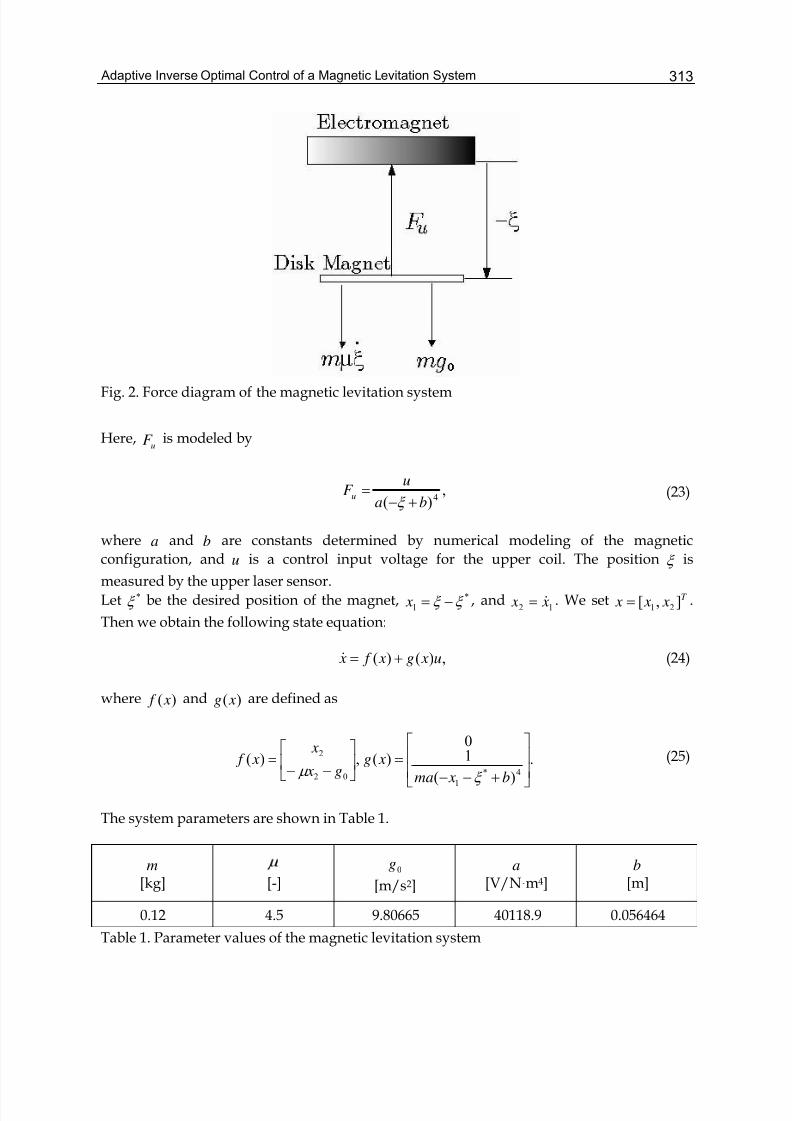
Adaptive Inverse Optimal Control of a Magnetic Levitation System 313
Fig. 2. Force diagram of the magnetic levitation system
Here,uF is modeled by
,)( 4ba
uF u +−
=ξ
(23)
where a and b are constants determined by numerical modeling of the magnetic
configuration, and u is a control input voltage for the upper coil. The position ξ is
measured by the upper laser sensor.
Let *ξ be the desired position of the magnet, *
1 ξ ξ −= x , and12 x x &= . We set T x x x ],[ 21= .
Then we obtain the following state equation:
,)()( u xg x f x +=& (24)
where )( x f and )( xg are defined as
.
)(
10
)(,)(4*
102
2
⎥⎥
⎦
⎤
⎢⎢
⎣
⎡
+−−=⎥
⎦
⎤⎢⎣
⎡
−−=
b xma
xgg x
x x f
ξ μ
(25)
The system parameters are shown in Table 1.
m
[kg] [-]0g
[m/s2]
a
[V/Nxm4]b
[m]
0.12 4.5 9.80665 40118.9 0.056464
Table 1. Parameter values of the magnetic levitation system
Adaptive Control314
There exists the following input constraint in system (24):
52
2<= uu [V]. (26)
By the above discussion, the control problem is reduced to the stabilization problem ofsystem (24) with the input constraint (26).
4. Pre-feedback Gravity Compensation
In system (2), we assume that 0)0( = f . However, 0)0( ≠ f in system (24). Therefore, we
cannot directly apply the inverse optimal controller (14) to system (24). To achieve 0)0( = f ,
we design a controller to compensate for gravity by a pre-feedback input.We consider the following gravity compensation input )( xuc
as
.)()(4*
10 b xamg xuc +−−= ξ (27)
Substituting (27) into (24), the gravitational acceleration0g is successfully canceled. Then,
we split the input )( xu using )( xucas
),()()( xu xu xu sc+= (28)
wheresu is an asymptotic stabilizing input for system (24) when 00 =g .
By using (26) and (28), the input constraint is rewritten to
.5)()()(22<+= xu xu xu sc
(29)
To handle input constraint (29) as a norm constraint, we rewrite (29) as
).(:)(5)(2
xC xu xu cs =−< (30)
(30) represents a constraint depending on the state. Note that constraint (30) is more severethan the original constraint (29). The problem of designing controller (28) is reduced to the
problem of designing controller )( xuswith input constraint )()(
2xC xus < .
To apply inverse optimal controller (14), we construct a CLF for system (24). In general, thecontroller performance often depends on a CLF. However, it is unclear which CLF achievesthe best control performance. Hence, we construct a CLF with a design parameter. Using theintegrator backstepping method, a CLF )( xV can be carried out as
,2
1)1(
2
1)(
2
221
2
1
2 x xrx xr xV +++= (31)
Adaptive Inverse Optimal Control of a Magnetic Levitation System 315
where r is a positive constant and also a design parameter.Now, we construct input
su . Let )(0 x f be the function defined by
.|)()(2
2
00 0 ⎥⎦
⎤⎢⎣
⎡
−== =
x
x x f x f g
μ (32)
By using (31), we can calculate V L f 0and V Lg
as
,)()1(2
221
2
0 xr x xr r V L f μ μ −+−+= (33)
.)( 4*
1
21
b xma
xrxV Lg +−−
+=
ξ (34)
Substituting (33) and (34) into (14) and (15), we get the following input )( xus.
,)(
1)(
1
V L x R
xu gs −= ,(35)
⎪⎪
⎩
⎪⎪
⎨
⎧
=
≠++
+
=
),0()(
2
)0()()(2
))(2(
)( 211
22
1
V L xq
V LV L xqPP
V LV L xq
x R
g
g
g
gg
(36)
,)(
)(
2
10
V L xC
V L xP
g
f =
(37)
.)(5)()(2
xud xdC xq c−==
(38)
According to Theorem 2, )( xushas a sector margin ),2/1( ∞ .
Finally, the following controller )( xu is obtained:
.)(
1)()(
1
4*
10 V L x R
b xamg xu g−+−−= ξ (39)
5. Experiment 1
We apply controller (39) to the magnetic levitation system. We set [ ]T x 0.0,4.1)0( −= and
0.2* −=ξ [cm]. The controller is implemented by MATLAB/SIMULINK. The sampling
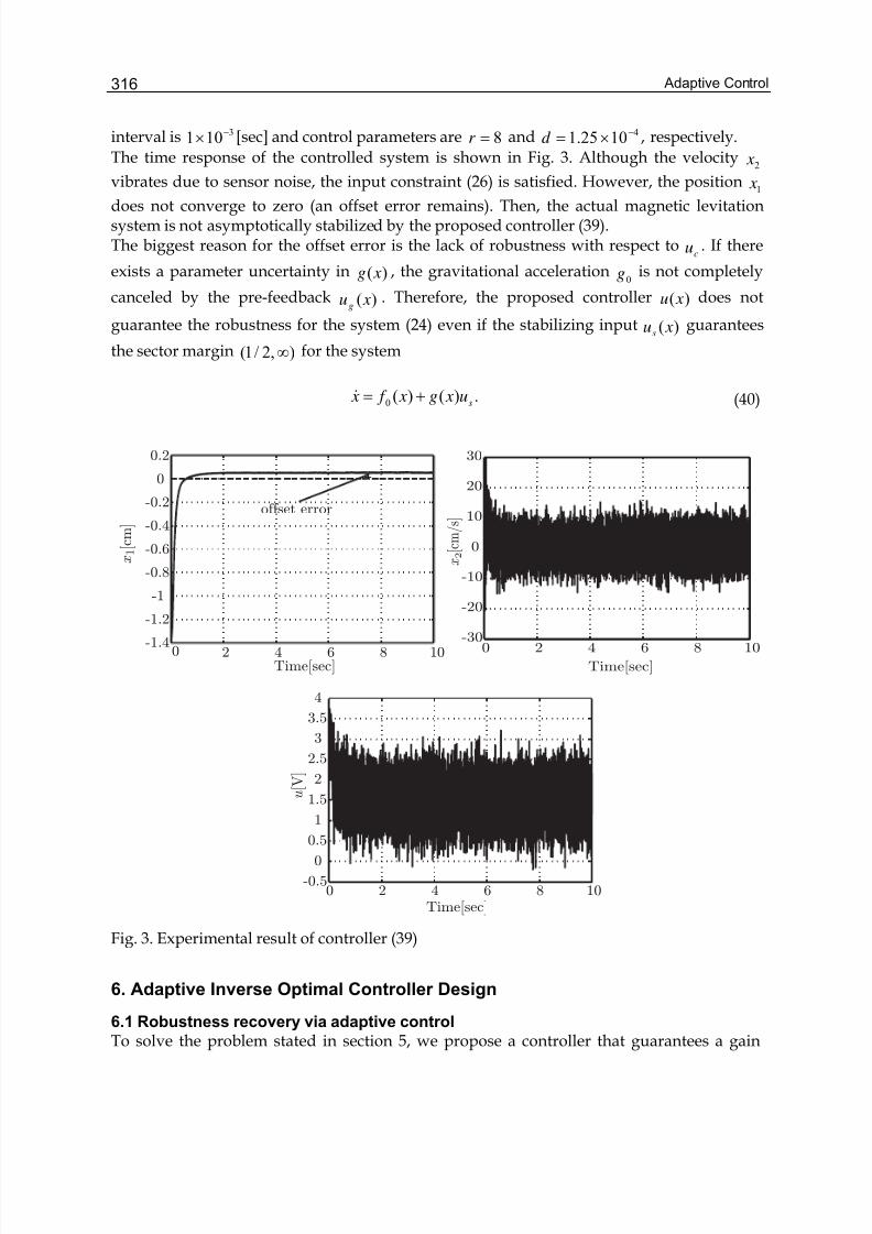
Adaptive Control316
interval is 3101 −× [sec] and control parameters are 8=r and 41025.1 −×=d , respectively.
The time response of the controlled system is shown in Fig. 3. Although the velocity2 x
vibrates due to sensor noise, the input constraint (26) is satisfied. However, the position1 x
does not converge to zero (an offset error remains). Then, the actual magnetic levitationsystem is not asymptotically stabilized by the proposed controller (39).The biggest reason for the offset error is the lack of robustness with respect to
cu . If there
exists a parameter uncertainty in )( xg , the gravitational acceleration0g is not completely
canceled by the pre-feedback )( xug. Therefore, the proposed controller )( xu does not
guarantee the robustness for the system (24) even if the stabilizing input )( xusguarantees
the sector margin ),2/1( ∞ for the system
.)()(0 su xg x f x +=& (40)
Fig. 3. Experimental result of controller (39)
6. Adaptive Inverse Optimal Controller Design
6.1 Robustness recovery via adaptive control
To solve the problem stated in section 5, we propose a controller that guarantees a gain
0 2 4 6 8 10-1.4
-1.2
-1
-0.8
-0.6
-0.4
-0.2
0
0.2
Time[sec]
x 1
[ c m
]
offset error
0 2 4 6 8 10-30
-20
-10
0
10
20
30
Time[sec]
x 2
[ c m
/ s ]
0 2 4 6 8 10-0.5
0
0.5
1
1.5
2
2.5
3
3.5
4
Time[sec]
u [ V ]
Adaptive Inverse Optimal Control of a Magnetic Levitation System 317
margin for u . We apply an adaptive control technique to achieve a gain margin for input u .
Before applying the adaptive controller, we rewrite the system (24) to
,)()()( 010 u xgg x f x f x ++=& (41)
where )(0 x f is defined by (31) and [ ]T x f 1,0)(1 −= . Additionally, to consider a gain margin
for (41), we rewrite the system to
,)()()( 10 u xg x f x f x κ θ κ ++=& (42)
where κ is an unknown constant and κ θ /: 0g= is a constant unknown parameter. Note
that the range of κ , in which the origin of the system (42) is asymptotically stable, is a gainmargin for input u . Furthermore, we consider the following input:
),ˆ,()ˆ,()ˆ,( θ θ θ xu xu xu sc′+= (43)
where κ θ ˆ/:ˆ 0g= and κ is an estimate of κ . We suppose that input )ˆ,( θ xus′ asymptotically
stabilizes the system (40) and guarantees the gain margin ),2/1( ∞ . Let )ˆ,( θ xugbe a gravity
compensation input defined as follows:
.)(ˆ)ˆ,( 4*
1 b xma xuc +−−= ξ θ θ (44)
Remark 1 In this section, we do not mention whether the input constraints exist or not.
Then, we construct an adaptive law θ &
such that the input (43) stabilizes the system (42) and
show the input (43) has a gain margin ),2/1( ∞ .
In this section, we use an ACLF to construct an adaptive law. The following lemma isavailable for constructing an ACLF.
Lemma 1 We consider system (42). Let )( xV be a CLF for system (41). Then, )( xV is an
ACLF for system (42).
Proof: If )( xV is an ACLF for system (42), )( xV is a CLF for the following system:
,)()()( 10 u xgV
x f x f x κ θ
γ θ κ +⎟ ⎠
⎞⎜⎝
⎛ ∂
∂++=& (45)
where γ is a positive constant. Note that 0/ =∂∂ θ V , the above system is rewritten to
.)()()( 10 u xg x f x f x κ θ κ ++=& (46)
Adaptive Control318
Sytem (46) is asymptotically stabilized by the input
),()()( xu xu xu sc+=θ (47)
where )( xucand )( xus
are defined by (27) and (35) respectively. This implies all CLFs for
system (41) are ACLFs for system (42).
By Lemma 1, CLF (31) is applicable to an ACLF for system (42).
Lemma 2 We consider system (42) and assume that an ACLF )( xV for (42) is obtained. Let
)ˆ,( θ xV ′ be a function defined by
,~
2)()ˆ(
2)()ˆ,( 22 θ
γ
κ θ θ
γ
κ θ +=−+=′ xV xV xV (48)
where ∞<<κ 2/1 and θ θ θ ˆ:~
−= . Let the adaptive law θ &
be
).()(ˆ1 x f
x
V x
∂
∂== γ γτ θ
& (49)
Then, )ˆ,( θ xV ′ is a Lyapunov function for the closed loop system of (42).
Proof: Let the origin of system (42) be ),0()ˆ,( θ θ = x . Then, V ′ is a positive definite function.
Assume u is input (43) and note that θ θ && ˆ~
−= . Then,
( ) [ ])ˆ,()ˆ,()(ˆ)()()ˆ,( 10 θ θ θ κ θ xu xu xg x f x f x
V xV sc
′+++∂
∂=′&
[ ] .0)ˆ,()()(0 ≤′+∂
∂= θ κ xu xg x f
x
V s
(50)
Since the input )ˆ,( θ xus′ has a gain margin ),2/1( ∞ , )ˆ,( θ xV & ′ is less than or equal to zero.
Then )ˆ,( θ xV ′ is a Lyapunov function for the closed loop system of (42) and the origin
),0()ˆ,( θ θ = x is stable.
Remark 2 Lyapunov function (48) contains an unknown constant κ . However, it does notbecome a problem because both input (43) and adaptive law (49) do not contain κ .
Lemma 3 We consider system (42) and assume that an ACLF )( xV for (42) is obtained.
Then, if ∞<< κ 2/1 , )(0 ∞→→ t x and )(ˆ ∞→→ t θ θ are achieved by input (43) and
adaptive law (49).
Adaptive Inverse Optimal Control of a Magnetic Levitation System 319
Proof: By Lemma 2, we can construct a Lyapunov function )ˆ,( θ xV ′ (47) for system (41).
The input and the adaptive law are given by (42) and (48), respectively. Then, we obtain
)0(0)ˆ,( ≠≤′ x xV θ & because the input )ˆ,( θ xus′ has a gain margin ),2/1( ∞ . Let S be a set
defined by
,ˆ,,0)ˆ,()ˆ,(: R R x xV xS n ∈∈=′= θ θ θ &
.ˆ,0)ˆ,( R x x ∈== θ θ (51)
We show that the largest invariant set contained in S consists of only a point ),0()ˆ,( θ θ = x .
Consider the following solution of (42) belonging to S :
.0,0)( ≥≡ t t x (52)
Note that 0)ˆ,0( =′ θ su , we obtain the following equation for (42):
,)ˆ,0()0()0()0( 10 θ θ κ ug f f x ++=&
,)ˆ,()0()0(1 θ θ κ xug f c+=
,0)ˆ(1 ≡−= θ θ κ f
(53)
where 0≠κ and 0)0(1 ≠ f , we obtain θ θ ≡ˆ . On the other hand, if 0= x and θ θ ≠ˆ , we
obtain 0≠ x& by (50). Therefore, the largest invariant set contained in S is a set ),0( θ .
Finally, we obtain 0→ x and θ θ →ˆ when ∞→t by LaSalle’s invariance principle [Khalil
(2002)].
The following theorem is obtained by Lemmas 2 and 3.
Theorem 4 We consider system (42), controller (43) and adaptive law (49). Then, thecontroller has a gain margin ),2/1( ∞ .
6.2 Adaptive inverse optimal controller
We calculate θ &
of (49) by using CLF (31) as:
[ ] ⎥⎦
⎤⎢⎣
⎡
−+++=
1
0)1(ˆ
2121
2 xrxrx xr γ θ &
).( 21 xrx +−= γ
(54)
Furthermore, taking into consideration the input constraint, we obtain the followingcontroller:
Adaptive Control320
),ˆ,()(ˆ)ˆ,()ˆ,()ˆ,( 4*
1 θ ξ θ θ θ θ xub xma xu xu xu ssc′++−−=′+=
(55)
,)ˆ,(
1)ˆ,(
2
V L x R
xu gsθ
θ −=′ ,(56)
⎪⎪
⎩
⎪⎪
⎨
⎧
=
≠++
+
=
),0()ˆ,(
2
)0()ˆ,()(2
))ˆ,(2(
)ˆ,( 222
22
2
V L xq
V LV L xqPP
V LV L xq
x R
g
g
g
gg
θ
θ
θ
θ
(57)
,)ˆ,(
)ˆ,(
2
20
V L xC
V L xP
g
f
θ θ =
(58)
),ˆ,()ˆ,( θ θ xdC xq = (59)
,)ˆ,(5)ˆ,(2
θ θ xu xC c−= (60)
where we use )( xusgiven by (35) as )ˆ,( θ xus
′ . Then, note that the input constraint )( xC is
rewritten to )ˆ,( θ xC given by (60). According to Lemma 2 and the result of [Nakamura et al.
(2007)], we can show the input )ˆ,( θ xus′ minimizes the following cost function:
∫∞
′+=0
22 ,2
)ˆ,()ˆ,( dt u
x R xl J s
θ θ (61)
where
.)ˆ,(2
1)ˆ,(
0
2
22
V LV L x R
xl f g −=θ
θ (62)
It is obvious that a gain margin ),2/1( ∞ is guaranteed for controller (55) at least in the
neighborhood of the origin.
7. Experiment 2
In this section, we apply controller (55) to the magnetic levitation system and confirm itseffectiveness by the experiment. To consider the input constraint, we employ the followingadaptive law with projection instead of (54):
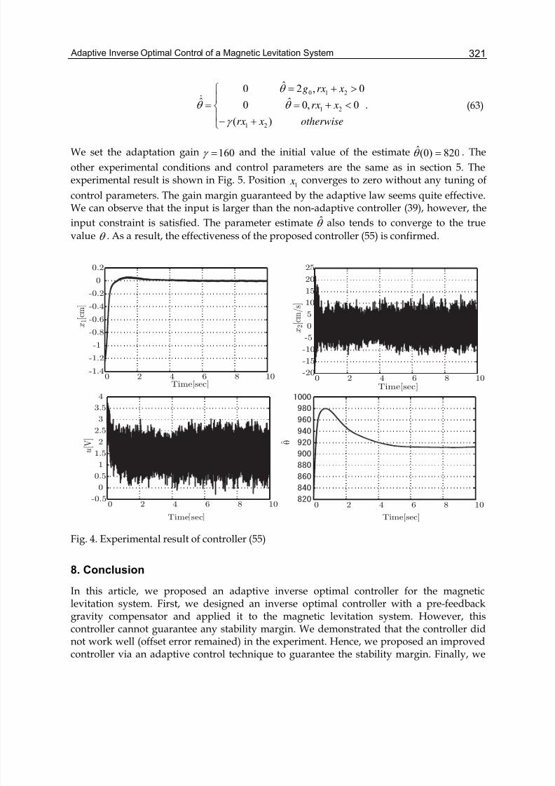
Adaptive Inverse Optimal Control of a Magnetic Levitation System 321
.0,0ˆ
0,2ˆ
)(
0
0
ˆ21
210
21 otherwise
xrx
xrxg
xrx
<+=
>+=
⎪⎩
⎪⎨
⎧
+−
= θ
θ
γ
θ &
(63)
We set the adaptation gain 160=γ and the initial value of the estimate 820)0(ˆ =θ . The
other experimental conditions and control parameters are the same as in section 5. Theexperimental result is shown in Fig. 5. Position
1 x converges to zero without any tuning of
control parameters. The gain margin guaranteed by the adaptive law seems quite effective.We can observe that the input is larger than the non-adaptive controller (39), however, the
input constraint is satisfied. The parameter estimate θ also tends to converge to the true
value θ . As a result, the effectiveness of the proposed controller (55) is confirmed.
Fig. 4. Experimental result of controller (55)
8. Conclusion
In this article, we proposed an adaptive inverse optimal controller for the magneticlevitation system. First, we designed an inverse optimal controller with a pre-feedbackgravity compensator and applied it to the magnetic levitation system. However, thiscontroller cannot guarantee any stability margin. We demonstrated that the controller didnot work well (offset error remained) in the experiment. Hence, we proposed an improvedcontroller via an adaptive control technique to guarantee the stability margin. Finally, we
0 2 4 6 8 10-1.4
-1.2
-1
-0.8
-0.6
-0.4
-0.2
0
0.2
Time[sec]
x 1
[ c m
]
0 2 4 6 8 10-20
-15
-10
-5
0
5
10
15
20
25
Time[sec]
x 2
[ c m
/ s ]
0 2 4 6 8 10-0.5
0
0.5
1
1.5
2
2.5
3
3.5
4
Time sec
u [ V ]
0 2 4 6 8 10
Time[sec]
θ ^
Adaptive Control322
confirmed the effectiveness of the proposed adaptive inverse optimal controller by theexperiment. As a result, we achieved offset-free control performance.
9. References
Freeman, R.A. & Kokotović, P.V. (1996). Robust Nonlinear Control Design. State-space andLyapunov Techniques. Birkhäuser, Boston.
Khalil, H.K. (2007). Nonlinear systems, 3rd ed. Prentice Hall, Upper Saddle River, New Jersey.Krstić, M.; Kanellakopoulos, I. & Kokotović, P. (1995). Nonlinear and Adaptive Control
Design. Wiley-Interscience, New York.Krstić, M. & Li, Z. (1998). Inverse optimal design of input-state-stabilizing nonlinear
controllers. IEEE Transaction on Automatic Control, 43, 3, 336-350.Li, Z. & Krstić, M. (1997). Optimal design of adaptive tracking controllers for non-linear
systems. Automatica, 33, 8, 1459-1473Mizutani, T.; Katayama, H. & Ichikawa A. (2004). Tracking control of a magnetic levitation
system by feedback linearization. Proceedings of SICE Annual Conference 2004, 121-126.
Nakamura, N. ; Nakamura, H.; Yamashita, Y. & Nishitani, H. (2007). Inverse optimal controlfor nonlinear systems with input constraints. Proceedings of the European ControlConference 2007 (CD-ROM).
Sepulchre, R.; Janković, M. & Kokotović, P.V. (1997). Constructive Nonlinear Control. Springer,London.
Sontag, E.D. (1989). A universal construction of Artstein’s theorem on nonlinear stabilization.System & Control Letters, 13, 117-123.
15
Adaptive Precision Geolocation Algorithm withMultiple Model Uncertainties
Wookjin Sung , Kwanho YouSungkyunkwan University, Department of Electrical Engineering
Korea
1. Introduction
In the unmanned ground vehicle (UGV) case, the estimation of a future position with apresent one is one of the most important techniques (Madhavan & Schlenoff, 2004).Generally, the famous global positioning system (GPS) has been widely used for positiontracking because of its good performance (Torrieri, 1984; Kim et al., 2006). However, thereexist some defects. For example, it needs a separate receiver and it must have at least threeavailable satellite signals. Moreover it is also vulnerable to the indoor case (Gleanson, 2006)or the reflected signal fading.There have been many researches to substitute or to assist the GPS. One of them is themethod of using the time difference of arrival (TDoA) which needs no special equipmentand can be operated in indoor multipath situation (Najar & Vidal, 2001). The TDoA meansan arrival time difference of signals transmitted from a mobile station to each base station. Itis the basic concept of estimation that the position of a mobile station can be obtained fromthe crossing point of hyperbolic curves which are derived from the definition of TDoA.Including some uncertainties, there have been several approaches to find the solution ofTDoA based geolocation problem using the least square method, for example, Tayler seriesmethod (Xiong et al., 2003), Chan’s method (Ho & Chan, 1993), and WLS method (Liu et al.,2006). However in case of a moving source, it demands a huge amount of computationalefforts each step, so it is required to use a method which demands less computational time.As a breakthrough to this problem, the application of EKF can be reasonable.The modeling errors happen in the procedure of linear approximation for system behaviorsto track the moving source’s position. The divergence caused from the modeling errors is acritical problem in Kalman filter applications (Julier & Uhlmann, 2004). The standardKalman filter cannot ensure completely the error convergence because of the limitedknowledge of the system’s dynamical model and the measurement noise. In realcircumstances, there are uncertainties in the system modeling and the noise description, andthe assumptions on the statistics of disturbances could be restrictive since the availability ofa precisely known model is very limited in many practical situations. In practical trackingfilter designs, there exist model uncertainties which cannot be expressed by the linear state-space model. The linear model increases modeling errors since the actual mobile stationmoves in a non-linear process. Especially even with a little priori knowledge it is quite
Adaptive Control324
valuable concerning the strategy.Hence, the compensation of model uncertainties is an important task in the navigation filterdesign. In modeling or formulating the mathematical equations, the possible predictionerrors are approximated or assumed as a model uncertainty. The facts discussed above leadsto unexpected deterioration of the filtering performance. To prevent the divergence problemdue to modeling errors in the EKF approach, the adaptive filter algorithm can be one of thegood strategies for estimating the state vector. This chapter suggests the adaptive fadingKalman filter (AFKF) (Levy, 1997; Xia et al., 1994) approach as a robust solution. The AFKFessentially employs suboptimal fading factors to improve the tracking capability. In AFKFmethod, the scaling factor is introduced to provide an improved state estimation. Thetraditional AFKF approach for determining the scaling factors mainly depends on thedesigner’s experience or computer simulation using a heuristic searching plan. In order toresolve this defect, the fuzzy adaptive fading Kalman filter (FAFKF) is proposed and used asan adaptive geolocation algorithm. The application of fuzzy logic to adaptive Kalmanfiltering gains more interests. The fuzzy logic adaptive system is constructed so as to obtainthe suitable scaling factors related to the time-varying changes in dynamics. In the FAFKF,the fuzzy logic adaptive system (FLAS) is used to adjust the scaling factor continuously soas to improve the Kalman filter performance.In this chapter, we also explain how to compose the FAFKF algorithm for TDoA basedposition tracking system. Through the comparison using the simulation results from theEKF and FAFKF solution under the model uncertainties, it shows the improved estimationperformance with more accurate tracking capability.
2. Geolocation with TDoA analytical methods
When the mobile station (MS: the unknown position) sends signals to each base station (BS:the known position), there is a time difference because of the BS’s isolated location from MS.The fundamental principle of position estimation is to use the intersection of hyperbolasaccording to the definition of TDoA as shown in Fig. 1.The problem of geolocation can be formulated as
1 1 1
=
= = −i i
i i i
d s b
d ct ct ct
-
, , 1, 2, 3, ,= = L
i i ib col x y i m
, = col x y
(1)
where ib is the known position of i-th signal receiver (BS), s is the unknown position of
signal source (MS), and c is the propagation speed of signal. In Eq. (1), id means the
distance between MS and i-th BS and it is the time of signal arrival (ToA) (Schau &
Robinson, 1987) from MS to i-th BS. Hence 1it becomes the time difference of arrival
(TDoA) which is the difference of ToA between it (from MS to the i-th BS) and 1t (from
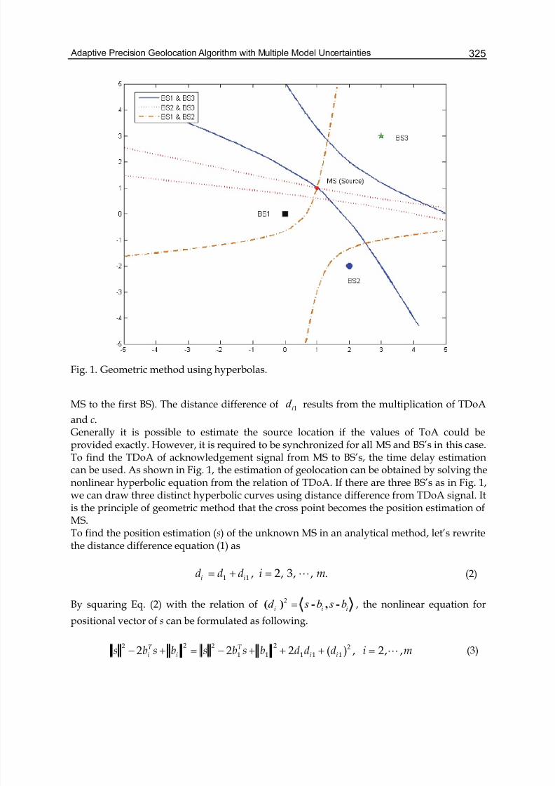
Adaptive Precision Geolocation Algorithm with Multiple Model Uncertainties 325
Fig. 1. Geometric method using hyperbolas.
MS to the first BS). The distance difference of 1id results from the multiplication of TDoA
and c.Generally it is possible to estimate the source location if the values of ToA could beprovided exactly. However, it is required to be synchronized for all MS and BS’s in this case.To find the TDoA of acknowledgement signal from MS to BS’s, the time delay estimationcan be used. As shown in Fig. 1, the estimation of geolocation can be obtained by solving thenonlinear hyperbolic equation from the relation of TDoA. If there are three BS’s as in Fig. 1,we can draw three distinct hyperbolic curves using distance difference from TDoA signal. Itis the principle of geometric method that the cross point becomes the position estimation ofMS.To find the position estimation (s) of the unknown MS in an analytical method, let’s rewritethe distance difference equation (1) as
1 1 , 2, 3, , .i id d d i m= + = L (2)
By squaring Eq. (2) with the relation of 2 =i i id s b s b( ) - , - , the nonlinear equation for
positional vector of s can be formulated as following.
2 22 2 21 1 1 1 12 2 2 ( ) , 2, ,T T
i i i is b s b s b s b d d d i m− + = − + + + = L (3)
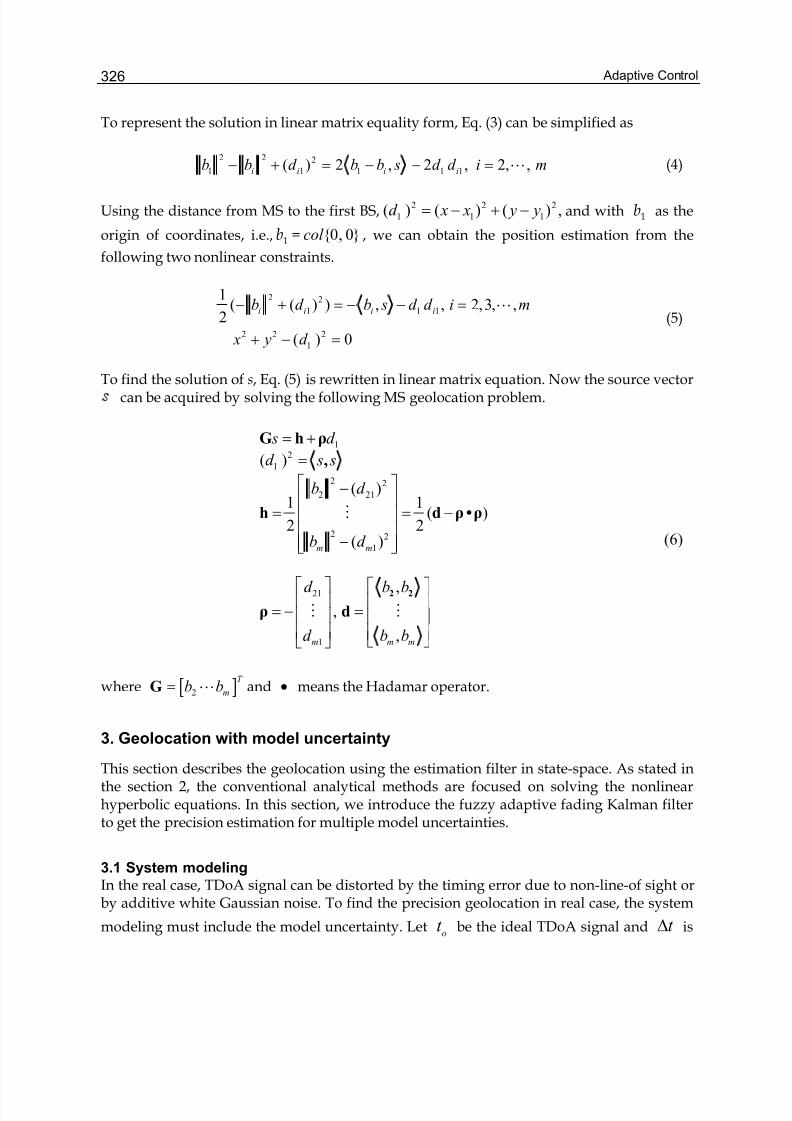
Adaptive Control326
To represent the solution in linear matrix equality form, Eq. (3) can be simplified as
2 2 2
1 1 1 1 1( ) 2 , 2 , 2, ,− + = − − = Li i i ib b d b b s d d i m (4)
Using the distance from MS to the first BS, 2 2 2
1 1 1( ) ( ) ( ) ,d x x y y= − + − and with 1b as the
origin of coordinates, i.e., 1b = 0, 0col , we can obtain the position estimation from the
following two nonlinear constraints.
2 2
1 1 1
2 2 2
1
1( ( ) ) , , 2,3, ,
2
( ) 0
i i i ib d b s d d i m
x y d
− + = − − =
+ − =
L (5)
To find the solution of s, Eq. (5) is rewritten in linear matrix equation. Now the source vectorcan be acquired by solving the following MS geolocation problem.
12
1
2 2
2 21
2 2
1
21
1
( )
( )1 1
( )2 2
( )
,
,
,
m m
m m m
s d
d s s
b d
b d
d b b
d b b
= +
=
⎡ ⎤−⎢ ⎥
= = −⎢ ⎥⎢ ⎥
−⎢ ⎥⎣ ⎦
⎡ ⎤ ⎡ ⎤⎢ ⎥ ⎢ ⎥
= − =⎢ ⎥ ⎢ ⎥⎢ ⎥ ⎢ ⎥⎣ ⎦⎣ ⎦
2 2
G h ρ
,
h d ρ •ρ
ρ d
M
M M
(6)
where [ ]2
T
mb b=G L and • means the Hadamar operator.
3. Geolocation with model uncertainty
This section describes the geolocation using the estimation filter in state-space. As stated inthe section 2, the conventional analytical methods are focused on solving the nonlinearhyperbolic equations. In this section, we introduce the fuzzy adaptive fading Kalman filterto get the precision estimation for multiple model uncertainties.
3.1 System modeling
In the real case, TDoA signal can be distorted by the timing error due to non-line-of sight orby additive white Gaussian noise. To find the precision geolocation in real case, the system
modeling must include the model uncertainty. Leto
t be the ideal TDoA signal and t Δ is
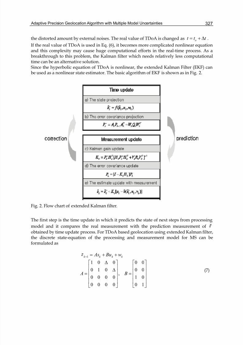
Adaptive Precision Geolocation Algorithm with Multiple Model Uncertainties 327
the distorted amount by external noises. The real value of TDoA is changed as = + Δot t t .
If the real value of TDoA is used in Eq. (6), it becomes more complicated nonlinear equationand this complexity may cause huge computational efforts in the real-time process. As abreakthrough to this problem, the Kalman filter which needs relatively less computationaltime can be an alternative solution.Since the hyperbolic equation of TDoA is nonlinear, the extended Kalman Filter (EKF) canbe used as a nonlinear state estimator. The basic algorithm of EKF is shown as in Fig. 2.
Fig. 2. Flow chart of extended Kalman filter.
The first step is the time update in which it predicts the state of next steps from processing
model and it compares the real measurement with the prediction measurement of ˆ
obtained by time update process. For TDoA based geolocation using extended Kalman filter,the discrete state-equation of the processing and measurement model for MS can beformulated as
1+ = + +k k k k As Bu w
1 0 0 0 0
0 1 0 0 0,
0 0 0 0 1 0
0 0 0 0 0 1
A B
Δ⎡ ⎤ ⎡ ⎤⎢ ⎥ ⎢ ⎥Δ⎢ ⎥ ⎢ ⎥= =⎢ ⎥ ⎢ ⎥⎢ ⎥ ⎢ ⎥⎣ ⎦ ⎣ ⎦
(7)
Adaptive Control328
where ( ) [ ]T k x y x y= & & , k u is the known velocity of moving MS, Δ is the time interval
of sampling, k w is an additive white Gaussian noise (AWGN).
From the definition of TDoA, the measurement model can be written as
( , )
1(|| || || ||)
=
= − − − +
k k k
k i k j k
z h s v
s b Ms b vc
1 0 0 0
0 1 0 0 M
⎡ ⎤= ⎢ ⎥⎣ ⎦
(8)
where ν k is the measurement noise in AWGN.
The output result of k which is the TDoA signal provides the information of MS position.
As an accurate geolocation method, the frequency difference (FDoA) resulted from Dopplershifts observation can be added in the state equation. However, to make the problem moresimple, we consider only the TDoA signal as an output measurement in this section.
Since the measurement model k z is nonlinear equation, the linear approximation using
partial differential method should be done for the use of EKF.
1
,
k k k k k
k k
k k
k k
z z H s V
h h H V
v
−= + +
∂ ∂≈ ≈∂ ∂
(9)
3.2 Geolocation using fuzzy adaptive fading Kalman filter (FAFKF)
EKF is a very useful method for nonlinear state estimation. However, as EKF is based on thelinearization of nonlinear system using partial differential method, the modeling errors caneasily lead to the divergence problem. To solve this problem, an adaptive fading Kalmanfilter (AFKF) with a fading factor can be applied. The application of AFKF to geolocationestimation is given in the following mathematical expression.
Basically, the fading factork
λ is added in the error covariance projection during the time
update process.
1λ −−= +T T
k k k k k k k k P A P A W Q W (10)
where 1 2( , , , )k mdiag λ λ λ λ = L . In normal case of 1λ =k , it means the general EKF. If the
estimated value approaches to the steady-state value, the fading factork
λ becomes less
than 1. Ifk
λ is greater than 1, the divergence could happen. This iterative process is called
as the adaptive fading loop given as follows.
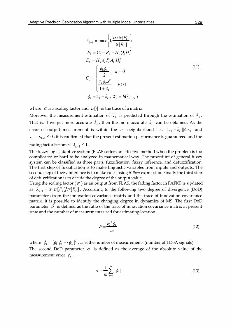
Adaptive Precision Geolocation Algorithm with Multiple Model Uncertainties 329
1
[ ]max 1,
[ ]
α λ +
⎧ ⎫⋅= ⎨ ⎬
⎩ ⎭
k
k
k
tr F
tr E
0= − − T
k k k k k F C R H Q H
= T T
k k k k k k E H A P A H
0 0
0
, 02
, 11
T
T
k k k
k
k
C
k
φ φ
λ φ φ
λ
⎧=⎪
⎪= ⎨⎪ ≥⎪ +⎩
ˆφ = −k k k z , ˆˆ ( , )=k k k h s v
(11)
where α is a scaling factor and [ ]tr ⋅ is the trace of a matrix.
Moreover the measurement estimation of ˆk
z is predicted through the estimation of ˆk .
That is, if we get more accurate ˆk , then the more accurate ˆ
k z can be obtained. As the
error of output measurement is within the ε − neighborhood i.e., ˆ|| || ε − ≤k k k z z and
1 0ε ε −− ≤k k , it is confirmed that the present estimation performance is guaranteed and the
fading factor becomes 1 1k λ + ≤ .
The fuzzy logic adaptive system (FLAS) offers an effective method when the problem is toocomplicated or hard to be analyzed in mathematical way. The procedure of general fuzzysystem can be classified as three parts; fuzzification, fuzzy inference, and defuzzification.The first step of fuzzification is to make linguistic variables from inputs and outputs. Thesecond step of fuzzy inference is to make rules using if-then expression. Finally the third stepof defuzzification is to decide the degree of the output value.Using the scaling factor (α ) as an output from FLAS, the fading factor in FAFKF is updated
as 1 [ ] [ ]λ α + = ⋅k k k tr F tr E . According to the following two degree of divergence (DoD)
parameters from the innovation covariance matrix and the trace of innovation covariancematrix, it is possible to identify the changing degree in dynamics of MS. The first DoD
parameter δ is defined as the ratio of the trace of innovation covariance matrix at present
state and the number of measurements used for estimating location.
φ φ δ =
T
k k
m (12)
where 1 2[ ]φ φ φ φ = LT
k m , m is the number of measurements (number of TDoA signals).
The second DoD parameter σ is defined as the average of the absolute value of the
measurement error k φ .
1
1| |σ φ
=
= ∑m
i
im (13)
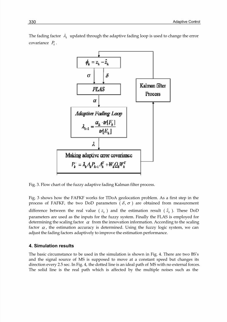
Adaptive Control330
The fading factor k λ updated through the adaptive fading loop is used to change the error
covariance k P .
Fig. 3. Flow chart of the fuzzy adaptive fading Kalman filter process.
Fig. 3 shows how the FAFKF works for TDoA geolocation problem. As a first step in theprocess of FAFKF, the two DoD parameters ( ,δ σ ) are obtained from measurement
difference between the real value ( k z ) and the estimation result ( ˆk z ). These DoD
parameters are used as the inputs for the fuzzy system. Finally the FLAS is employed fordetermining the scaling factor α from the innovation information. According to the scaling
factor α , the estimation accuracy is determined. Using the fuzzy logic system, we can
adjust the fading factors adaptively to improve the estimation performance.
4. Simulation results
The basic circumstance to be used in the simulation is shown in Fig. 4. There are two BS’sand the signal source of MS is supposed to move at a constant speed but changes itsdirection every 2.5 sec. In Fig. 4, the dotted line is an ideal path of MS with no external forces.The solid line is the real path which is affected by the multiple noises such as the
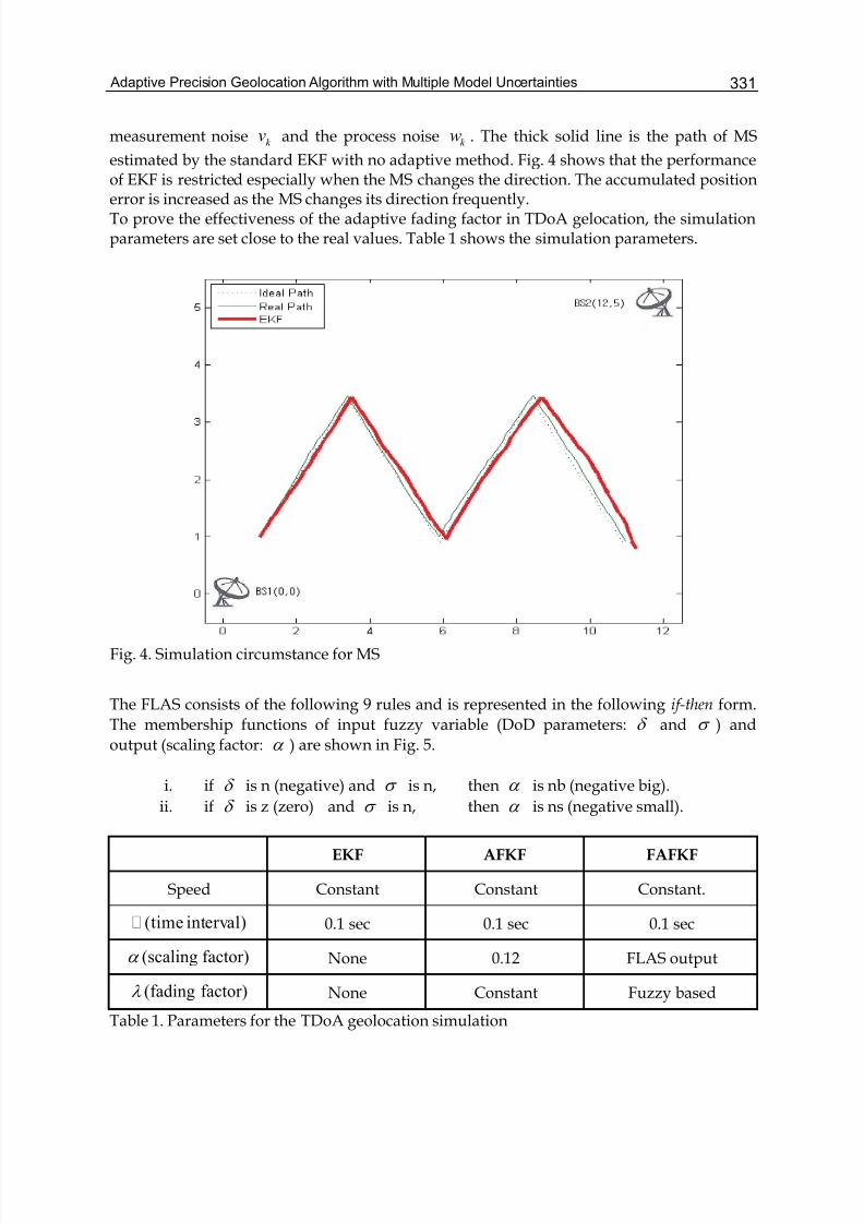
Adaptive Precision Geolocation Algorithm with Multiple Model Uncertainties 331
measurement noise k v and the process noise k w . The thick solid line is the path of MS
estimated by the standard EKF with no adaptive method. Fig. 4 shows that the performanceof EKF is restricted especially when the MS changes the direction. The accumulated positionerror is increased as the MS changes its direction frequently.To prove the effectiveness of the adaptive fading factor in TDoA gelocation, the simulationparameters are set close to the real values. Table 1 shows the simulation parameters.
Fig. 4. Simulation circumstance for MS
The FLAS consists of the following 9 rules and is represented in the following if-then form.
The membership functions of input fuzzy variable (DoD parameters: δ and σ ) and
output (scaling factor: α ) are shown in Fig. 5.
i. if δ is n (negative) and σ is n, then α is nb (negative big).
ii. if δ is z (zero) and σ is n, then α is ns (negative small).
EKF AFKF FAFKF
Speed Constant Constant Constant.
(time interval) 0.1 sec 0.1 sec 0.1 sec
(scaling factor)α None 0.12 FLAS output
(fading factor)λ None Constant Fuzzy based
Table 1. Parameters for the TDoA geolocation simulation
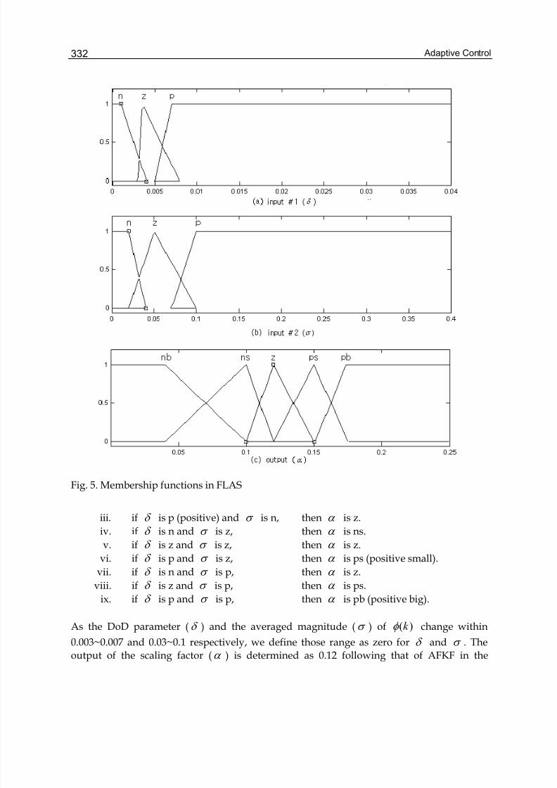
Adaptive Control332
Fig. 5. Membership functions in FLAS
iii. if δ is p (positive) and σ is n, then α is z.
iv. if δ is n and σ is z, then α is ns.
v. if δ is z and σ is z, then α is z.
vi. if δ is p and σ is z, then α is ps (positive small).
vii. if δ is n and σ is p, then α is z.
viii. if δ is z and σ is p, then α is ps.
ix. if δ is p and σ is p, then α is pb (positive big).
As the DoD parameter ( δ ) and the averaged magnitude (σ ) of ( )k φ change within
0.003~0.007 and 0.03~0.1 respectively, we define those range as zero for δ and σ . The
output of the scaling factor (α ) is determined as 0.12 following that of AFKF in the
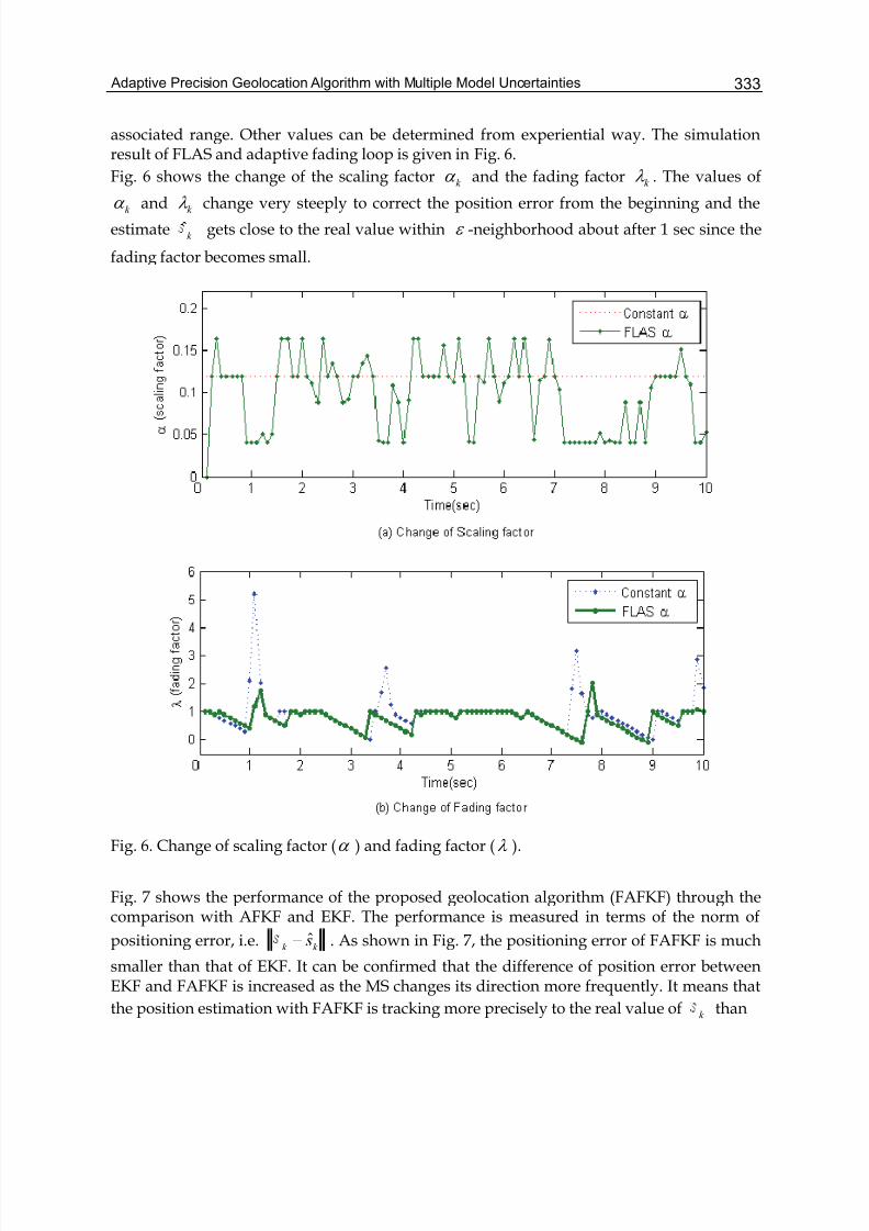
Adaptive Precision Geolocation Algorithm with Multiple Model Uncertainties 333
associated range. Other values can be determined from experiential way. The simulationresult of FLAS and adaptive fading loop is given in Fig. 6.
Fig. 6 shows the change of the scaling factor α k and the fading factor k λ . The values of
α k and k λ change very steeply to correct the position error from the beginning and the
estimate ˆk
gets close to the real value within ε -neighborhood about after 1 sec since the
fading factor becomes small.
Fig. 6. Change of scaling factor (α ) and fading factor (λ ).
Fig. 7 shows the performance of the proposed geolocation algorithm (FAFKF) through thecomparison with AFKF and EKF. The performance is measured in terms of the norm of
positioning error, i.e. ˆ−k k s . As shown in Fig. 7, the positioning error of FAFKF is much
smaller than that of EKF. It can be confirmed that the difference of position error betweenEKF and FAFKF is increased as the MS changes its direction more frequently. It means that
the position estimation with FAFKF is tracking more precisely to the real value of k than
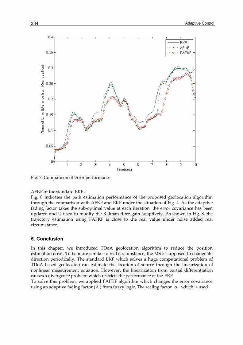
Adaptive Control334
Fig. 7. Comparison of error performance
AFKF or the standard EKF.Fig. 8 indicates the path estimation performance of the proposed geolocation algorithmthrough the comparison with AFKF and EKF under the situation of Fig. 4. As the adaptive fading factor takes the sub-optimal value at each iteration, the error covariance has beenupdated and is used to modify the Kalman filter gain adaptively. As shown in Fig. 8, thetrajectory estimation using FAFKF is close to the real value under noise added realcircumstance.
5. Conclusion
In this chapter, we introduced TDoA geolocation algorithm to reduce the positionestimation error. To be more similar to real circumstance, the MS is supposed to change itsdirection periodically. The standard EKF which solves a huge computational problem ofTDoA based geolocaion can estimate the location of source through the linearization ofnonlinear measurement equation. However, the linearization from partial differentiationcauses a divergence problem which restricts the performance of the EKF.To solve this problem, we applied FAFKF algorithm which changes the error covarianceusing an adaptive fading factor (λ )
from fuzzy logic. The scaling factor α which is used
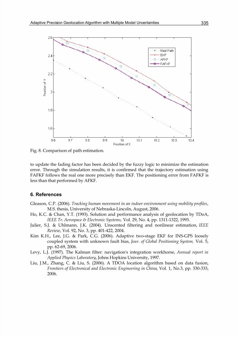
Adaptive Precision Geolocation Algorithm with Multiple Model Uncertainties 335
Fig. 8. Comparison of path estimation.
to update the fading factor has been decided by the fuzzy logic to minimize the estimationerror. Through the simulation results, it is confirmed that the trajectory estimation usingFAFKF follows the real one more precisely than EKF. The positioning error from FAFKF isless than that performed by AFKF.
6. References
Gleason, C.P. (2006). Tracking human movement in an indoor environment using mobility profiles,M.S. thesis, University of Nebraska-Lincoln, August, 2006.
Ho, K.C. & Chan, Y.T. (1993). Solution and performance analysis of geolocation by TDoA,IEEE Tr. Aerospace & Electronic Systems, Vol. 29, No. 4, pp. 1311-1322, 1993.
Julier, S.J. & Uhlmann, J.K. (2004). Unscented filtering and nonlinear estimation, IEEEReview, Vol. 92, No. 3, pp. 401-422, 2004.
Kim K.H., Lee, J.G. & Park, C.G. (2006). Adaptive two-stage EKF for INS-GPS looselycoupled system with unknown fault bias, Jour. of Global Positioning System, Vol. 5,pp. 62-69, 2006.
Levy, L.J. (1997). The Kalman filter: navigation's integration workhorse, Annual report in Applied Physics Laboratory, Johns Hopkins University, 1997.
Liu, J.M., Zhang, C. & Liu, S. (2006). A TDOA location algorithm based on data fusion,Frontiers of Electronical and Electronic Engineering in China, Vol. 1, No.3, pp. 330-333,2006.
Adaptive Control336
Madhavan, R. & Schlenoff, C. (2004). The effect of process models on short-term predictionof moving objects for unmanned ground vehicles, International IEEE Conf. IntelligentTransportation Systems, Vol. 1, pp. 471-476, 2004.
Najar, M. & Vidal, J. (2001). Kalman tracking based on TDOA for UMTS mobile location,IEEE International Symp. Personal, Indoor and Mobile Radio Communications, Vol. 1,pp. B45-B49, 2001.
Schau, H.C. & Robinson, A.Z. (1987). Passive source localization employing intersectingspherical surfaces from Time-of-Arrival differences, IEEE Tr. Acoustics, Speech, &Signal Processing, Vol. ASSP-35, No. 8, pp. 1223-1225, 1987.
Torrieri, D.J. (1984). Statistical theory of passive location systems, IEEE Tr. on Aerospace andElectronic Systems, Vol. AES-20, No. 2, pp. 183-197, 1984.
Xia, Q., Rao, M., Ying, Y. & Shen, X. (1994). Adaptive fading Kalman filter with anapplication, Automatica, Vol. 30, No. 8, pp. 1333-1338, 1994.
Xiong, J.Y., Wang, W. & Zhu, Z.L. (2003). An improved Taylor algorithm inTDOAsubscriber position location, Proc. of ICCT , Vol. 2, pp. 981-984, 2003.
16
Adaptive Control for a Class of Non-affineNonlinear Systems via Neural Networks
Zhao TongSchool of Automatization and Electronic Engineering, Qingdao University of Science and
TechnologyChina
1. Introduction
Adaptive control of highly uncertain nonlinear dynamic systems has been an importantresearch area in the past decades, and in the meantime neural networks control has foundextensive application for a wide variety of areas and has attracted the attention of manycontrol researches due to its strong approximation capability. Many significant results onthese topics have been published in the literatures (Lewis et al., 1996 ; Yu & Li 2002;Yesidirek & Lewis 1995). It is proved to be successful that neural networks are used inadaptive control. However, most of these works are applicable for a kind of affine systemswhich can be linearly parameterized. Little has been found for the design of specificcontrollers for the nonlinear systems, which are implicit functions with respect to controlinput. We can find in literatures available there are mainly the results of Calise et al. (Calise& Hovakimyan 2001) and Ge et al. (Ge et al. 1997). Calise et al. removed the affine in controlrestriction by developing a dynamic inversion based control architecture with linearlyparameterized neural networks in the feedback path to compensate for the inversion errorintroduced by an approximate inverse. However, the proposed scheme does not relate to theproperties of the functions, therefore, the special properties are not used in design. Ge, S.S.et al., proposed the control schemes for a class of non-affine dynamic systems, using meanvalue theorem, separate control signals from controlled plant functions, and apply neuralnetworks to approximate the control signal, therefore, obtain an adaptive control scheme.Furthermore, when controlling large-scale and highly nonlinear systems, the presuppositionof centrality is violated due to either due to problems in data gathering when is spread outor due to the lack of accurate mathematical models. To avoid the difficulties, thedecentralized control architecture has been tried in controller design. Decentralized controlsystems often also arise from various complex situations where there exist physicallimitations on information exchange among several subsystems for which there isinsufficient capability to have a single central controller. Moreover, difficulty anduncertainty in, measuring parameter values within a large-scale system may call foradaptive techniques. Since these restrictions encompass a large group of applications, avariety of decentralized adaptive techniques have been developed (Ioannou 1986).
Adaptive Control338
Earlier literature on the decentralized control methods were focused on control of large-scale linear systems. The pioneer work by Siljak (Siljak 1991) presents stability theorems ofinterconnected linear systems based on the structure information only. Many worksconsider subsystems which are linear in a set of unknown parameters (Ioannou 1986 ; Fu1992 ; Sheikholeslam & Desor 1993 ; Wen 1994 ; Tang et al. 2000), and these results werefocused on systems with first order interconnections. When the subsystems has nonlineardynamics or the interconnected is entered in a nonlinear fashion, the analysis and designproblem becomes even challenging.The use of neural networks’ learning ability avoids complex mathematical analysis insolving control problems when plant dynamics are complex and highly nonlinear, which isa distinct advantage over traditional control methods. As an alternative, intensive researchhas been carried out on neural networks control of unknown nonlinear systems. Thismotivates some researches on combining neural networks with adaptive control techniquesto develop decentralized control approaches for uncertain nonlinear systems withrestrictions on interconnections. For example, in (Spooner & Passino 1999), twodecentralized adaptive control schemes for uncertain nonlinear systems with radial basisneural networks are proposed, which a direct adaptive approach approximates unknowncontrol laws required to stabilize each subsystem, while an indirect approach is providedwhich identifies the isolated subsystem dynamics to produce a stabilizing controller. For aclass of large scale affine nonlinear systems with strong interconnections, two neuralnetworks are used to approximate the unknown subsystems and strong interconnections,respectively (Huang & Tan 2003), and Huang & Tan (Huang & Tan 2006) introduce adecomposition structure to obtain the solution to the problem of decentralized adaptivetracking control a class of affine nonlinear systems with strong interconnections. Apparently,most of these results are likewise applicable for affine systems described as above. For thedecentralized control research of non-affine nonlinear systems, many results can be foundfrom available literatures. Nardi et al. (Nardi & Hovakimyan 2006) extend the results inCalise et al. (Calise & Hovakimyan 2001) to non-affine nonlinear dynamical systems withfirst order interconnections. Huang (Huang & Tan 2005) apply the results in (Ge & Huang1999) to a class of non-affine nonlinear systems with strong interconnections.Inspired by the above researches, in this chapter, we propose a novel adaptive controlscheme for non-affine nonlinear dynamic systems. Although the class of nonlinear plant isthe same as that of Ge et al. (Ge et al. 1997), utilizing their nice reversibility, and invokingthe concept of pseudo-control and inverse function theorem, we find the equitation of errordynamics to design adaptation laws. Using the property of approximation of two-layerneural networks (NN), the control algorithm is gained. Then, the controlled plants areextended to large-scale decentralized nonlinear systems, which the subsystems arecomposed of the class of non-affine nonlinear functions. Two schemes are proposed,respectively. The first scheme designs a RBFN-based (radial basis function neural networks)adaptive control scheme with the assumption which the interconnections betweensubsystems in entire system are bounded linearly by the norms of the tracking filtered error.In the scheme, unlike most of other approaches in available literatures, the weight of BBFNand center and width of Gaussian function are tuned adaptively. In another scheme, theinterconnection is assumed as stronger nonlinear function. Moreover, in the former, in everysubsystem, a RBFN is adopted which is used to approximate unknown function, and in thelatter, in every subsystem, two RBFNs are respectively utilized to approximate unknown
Adaptive Control for a Class of Non-affine Nonlinear Systems via Neural Networks 339
function and uncertain strong interconnection function. For those complicated large-scaledecentralized dynamic systems, in order to decrease discontinuous factors and makesystems run smooth, unlike most of control schemes, the hyperbolic tangent functions arequoted in the design of robust control terms, instead of sign function. Otherwise, the citationof the smooth function is necessary to satisfy the condition of those theorems.The rest of the paper is organized as follows. Section 2 gives the normal form of a class ofnon-affine nonlinear systems. Section 3 proposes a novel adaptive control algorithm, whichis strictly derived from some mathematical and Lyapunov stability theories, and theeffectiveness of the scheme is validated through simulation. Extending the above-mentionedresult, Section 4 discusses two schemes of decentralized adaptive neural network control forthe class of large-scale nonlinear systems with linear function interconnections andnonlinear function interconnections, respectively. Finally, the Section 5 is concludingremarks.
2. Problem Statement
We consider a general analytic system
( , ), ,
( ), .
nu R u R
y h y R
⎧ = ∈ ∈⎨
= ∈⎩
ζ g ζ ζ
ζ
&(1)
where ( , )⋅ ⋅g is a smooth vector fields and ( )h ⋅ is a scalar function. In practice, many
physical systems such as chemical reactions, PH neutralization and distillation columns areinherently nonlinear, whose input variables may enter in the systems nonlinearly asdescribed by the above general form (Ge et al. 1998). Then, the Lie derivative (Tsinias &
Kalouptsidis 1983) of ( )h ζ with respect to ( , )ug ζ is a scalar function defined
by [ ( ) ] ( , ) L h h u= ∂ ∂g
ζ ζ g ζ . Repeated Lie derivatives can be defined recursively
as 1( ), 1,2i i L h L L h for i−= =g g g L . The system (1) is said to have relative degree α
at0( , )u0
ζ , if there exists a smallest positive integer α such
that 0i L h u∂ ∂ =g, 1, , 10, i L h uα
α = −∂ ∂ ≠g L .
LetnΩ ⊂ζ and u RΩ ⊂ be compact subsets containing
0ζ and 0u , respectively. System
(1) is said to have a strong relative degree α in a compact setu
D = Ω ×Ωζ, if it has relative
degree α at every point0( , )u D∈0ζ . Therefore, system (1) is feedback linearizable and the
mapping1 2( ) [ ( ), ( ), ( )]nφ φ φ Φ =ζ ζ ζ ζL , with 1( ) , 1, 2, j
j L h jφ α −= =gζ L has a Jacobian
matrix which is nonsingular for all ( )∈Φx ζ , system (1) can be transformed into a normal
form
Adaptive Control340
1 2
2 3
1
( , )n
x x
x x
x f x u
y x
=⎧⎪ =⎪⎪⎨⎪ =⎪
=⎪⎩
&
&
M
&
(2)
where ( , ) n f x u L h=g
and1( ) x −= Φ ζ with 1 2[ , , , ]T
n x x x x= L . Define the domain of
normal system (2) as ( , ) ( ); u D x u x u∈Φ Ω ∈Ωζ .
3. Adaptive Control for a Class of Non-affine Nonlinear Systems via Two-Layer Neural Networks
Now we consider the n th− order nonlinear systems of the described form as (2). For the
considered systems in the chapter, we may make the following assumptions.
Assumption 1. ( , ) / 0 f x u u∂ ∂ ≠ for all ( , ) x u R∈Ω× .
Assumption 2. 1( ) : n f R R+⋅ → , is an unknown continuous function and ( , ) f x u a smooth
function with respect to control input u .
The control objective is: determine a control law, force the output, y , to follow a given
desired output, d x with an acceptable accuracy, while all signals involved must be
bounded.
Assumption 3. The desired signals (1) ( 1)( ) [ , , , ],n
d d d d x t y y y −= L and ( )[ , ]T n T
d d d X x y= are
bounded, withd X X ≤d
,d X a known positive constant.
Define the tracking error vector as
d e x x= − , (3)
and a filtered tracking error as
[ 1]T eτ = Λ , (4)
with Λ a gain parameter vector selected so that ( ) 0e t → as 0.τ → Differentiating (4), the
filtered tracking error can be written as
( ) [0 ] .n T
n d x xτ = − + Λ e& & (5)
Define a continuous function
Adaptive Control for a Class of Non-affine Nonlinear Systems via Neural Networks 341
( ) [0 ] .n T
d k xδ τ = − + − Λ e (6)
where k is a positive constant. We know ( , ) 0 f x u u∂ ∂ ≠ (Assumption 1), thus,
[ ( , ) ] 0 f x u uδ ∂ − ∂ ≠ . Considering the fact that 0uδ ∂ ∂ = , we invoke the implicit
function theorem (Lang 1983), there exists a continuous ideal control input u∗in a
neighborhood of ( , ) x u R∈Ω× , such that ( , ) 0 f x u δ ∗ − = , i.e. ( , ) x uδ ∗= holds.
( , ) f x uδ ∗= may represent ideal control inverse.
Adding and subtracting δ to the right-hand side of ( , )n
f x u=& of (2), one obtains
( )( , ) [0 ]n T
n d x f x u k x eδ τ = − − + − Λ& , (7)
and yields
( , ) .k f x uτ τ δ = − + −& (8)
Considering the following state dependent transformationn
xψ = & , whereψ is commonly
referred to as the pseudo-control (Calise & Hovakimyan 2001). Apparently, the pseudo-control is not a function of the control u but rather a state dependent operator.
Then, 0uψ ∂ ∂ = , from Assumption 1, ( , ) 0 f x u u∂ ∂ ≠ thus [ ( , )] 0 f x u uψ − ∂ ≠ .
With the implicit function theorem, for every ( , ) x u R∈Ω× , there exists a implicit
function such that ( , ) 0 f x uψ − = holds, i.e. ( , ) f x uψ = . Therefore, we have
( , ) f x uψ = . (9)
Furthermore, using inverse function theorem, with the fact that [ ( , )] 0 f x u uψ − ∂ ≠
and ( , ) f x u is a smooth with respect to control input, u , then, ( , ) x u defines a local
diffeomorphism (Slotine & Li 1991), such that, for a neighborhood of u , there exists a
smooth inverse function and1( , )u f x ψ −= holds. If the inverse is available, the control
problem is easy. But this inverse is not known, we can generally use some techniques, suchas neural networks, to approximate it. Hence, we can obtain an estimated function,
1 ˆˆ ( , )u f x ψ −= . This result in the following equation holding:
ˆ ˆ( , ) x uψ = , (10)
where ψ may be referred to as approximation pseudo-control input which represents
actual dynamic approximation inverse.
Adaptive Control342
Remark 1. According to the above-mentioned conditions, when one designs the pseudo-
control signal, ψ , must be a smooth function. Therefore, in order to satisfy the condition,
we adopt hyperbolic tangent function, instead of sign function in design of input. This alsomakes control signal tend smooth and system run easier. The hyperbolic tangent functionhas a good property as follows (Polycarpou 1996) :
0 tanh( )η
η η ςα α
< − ≤ , (11)
with 0.2785ς = , α any positive constant. Moreover, theoretically, ψ is approximation
inverse, generally a nonlinear function, but it must be bounded and play a dynamicapproximation role and make system stable. Hence, it represents actual dynamicapproximation inverse.Based on the above conditions, in order to control the system and make it be stable, we
design the approximation pseudo-control input ψ as follows:
ˆ ( , ) ad r f x u u vψ ∗= + + , (12)
where ad u is output of a neural network controller, which adopts a two-layer neural
network,r
v is robustifying control term designed in stability analysis.
Adding and subtracting ψ to the right-hand side of (8), with ( , ) x uδ ∗= , we have
ˆ( , ) ( , )
ˆ( , , ) ,
ad r
ad r
k f x u f x u u v
k x u u u v
τ τ ψ δ
τ ψ δ
∗
∗
= − + + − − − −
= − + Δ + − − −
&
%(13)
where ( , , ) ( , ) ( , )u u f x u f x u∗ ∗Δ = −% is error between nonlinear function and its ideal
control function, we can use the neural network to approximate it.
3.1 Neural network-based approximationA two-layer NN consists of two layers of tunable weights, a hidden layer and an output
layer. Given a 0ε > , there exists a set of bounded weights and N such that the
nonlinear error ( )C Δ∈ Ω% , with Ω compact subset ofn
, can be approximated by a two-
layer neural network, i.e.
( ) ( )T T
nn nn N x xσ ε Δ = +% , (14)
with ˆ[1, , , ]T T
nn d x x e ψ = input vector of NN.
Adaptive Control for a Class of Non-affine Nonlinear Systems via Neural Networks 343
Assumption 4. The approximation error ε is bounded as follows:
N ε ε ≤ , (15)
where 0 N ε > is an unknown constant.
Let ˆ and ˆ N be the estimates respectively of and N . Based on these estimates, let
ad u be the output of the NN
ˆ ˆ( ).T T
ad nnu M N xσ = (16)
Define ˆ M M = −% and ˆ N N N = −% , where we use notations: [ , ] Z diag M N = ,
[ , ] Z diag M N =% % % , ˆ ˆ ˆ[ , ] Z diag M N = for convenience. Then, the following inequality
holds:
2ˆ( )T
F F F tr Z Z Z Z Z ≤ −% % % . (17)
The Taylor series expansion of ( )T
nn N xσ for a given
nn x can be written as:
2ˆ ˆ( ) ( ) ( ) ( )T T T T T
nn nn nn nn nn N x N x N x N x O N xσ σ σ ′= + +% % , (18)
with ˆˆ : ( )T
nn N xσ σ = and σ ′ denoting its Jacobian, 2( )T
nnO N x% the term of order two. In
the following, we use notations: : ( )T
nn N xσ σ = , : ( )T
nn N xσ σ = %% .
With the procedure as Appendix A, the approximation error of function can be written as
ˆ ˆ ˆˆ ˆ ˆ( ) ( ) ( )T T T T T T T T
nn nn nn nn M N x M N x M N x M N xσ σ σ σ σ ω ′ ′− = − + +% % , (19)
and the disturbance term ω can be bounded as
1ˆ ˆˆ ˆT T
nn nn F F N x M M N x M ω σ σ ′ ′≤ + + , (20)
where the subscript “F” denotes Frobenius norm, and the subscript “1” the 1-norm.Redefine this bound as
ˆ ˆ( , , )nn N xω ω ω ρ ϑ ≤ , (21)
Adaptive Control344
where1
max , , F
M N M ω ρ = and ˆ ˆˆ ˆ 1T T
nn nn F
x M N xω ϑ σ σ ′ ′= + + . Notice that
ω ρ is an unknown coefficient, whereasω ϑ is a known function.
3.2 Parameters update law and stability analysisSubstituting (14) and (16) into (13), we have
ˆ ˆ ˆ( ) ( ) ( ).T T T T
nn nn r nnk M N x M N x v xτ τ σ σ ψ δ ε = − + − + − − +& (22)
Using(19), the above equation can become
ˆ ˆ ˆˆ ˆ ˆ( ) .T T T T
nn nn r k M N x M N x vτ τ σ σ σ ψ δ ω ε ′ ′= − + − + + − − + +% %& (23)
Theorem 1. Consider the nonlinear system represented by Eq. (2) and let Assumption 1-4
hold. If choose the approximation pseudo-control input ψ as Eq.(12), use the following
adaptation laws and robust control law
1
1
ˆ ˆˆ ˆ( ) ,
ˆ ˆ ˆˆ ,
( 1)ˆ ˆ( 1) tanh
( 1)ˆ( 1) tanh
nn
T
nn
r
M F Nx k M
N R x M k N
v
ω ω
ω ω
σ σ τ τ
σ τ τ
τ ϑ φ γ τ ϑ λφ
α
τ ϑ φ ϑ
α
⎡ ⎤′= − −⎣ ⎦
⎡ ⎤′= −⎣ ⎦
⎧ + ⎫⎡ ⎤= + −⎨ ⎬⎢ ⎥
⎣ ⎦⎩ ⎭
+⎡ ⎤= − + ⎢ ⎥
⎣ ⎦
&
&
&
(24)
where 0, 0T T F F R R= > = > are any constant matrices, 1 0k > and 0γ > are scalar
design parameters, φ is the estimated value of the uncertain disturbance term
max( , ) N ω φ ρ ε = , defining ˆφ φ φ = −% with φ % error ofφ , then, guarantee that all signals
in the system are uniformly bounded and that the tracking error converges to aneighborhood of the origin.Proof. Consider the following positive define Lyapunov function candidate as
2 1 1 1 21 1 1 1( ) ( )
2 2 2 2
T T L tr M F M tr N R N τ γ φ − − −= + + + %% % % % (25)
The time derivative of the above equation is given by
1 1 1( ) ( )T T L tr M F M tr N R N ττ γ φφ − − −= + + + && & % %& % % % %& (26)
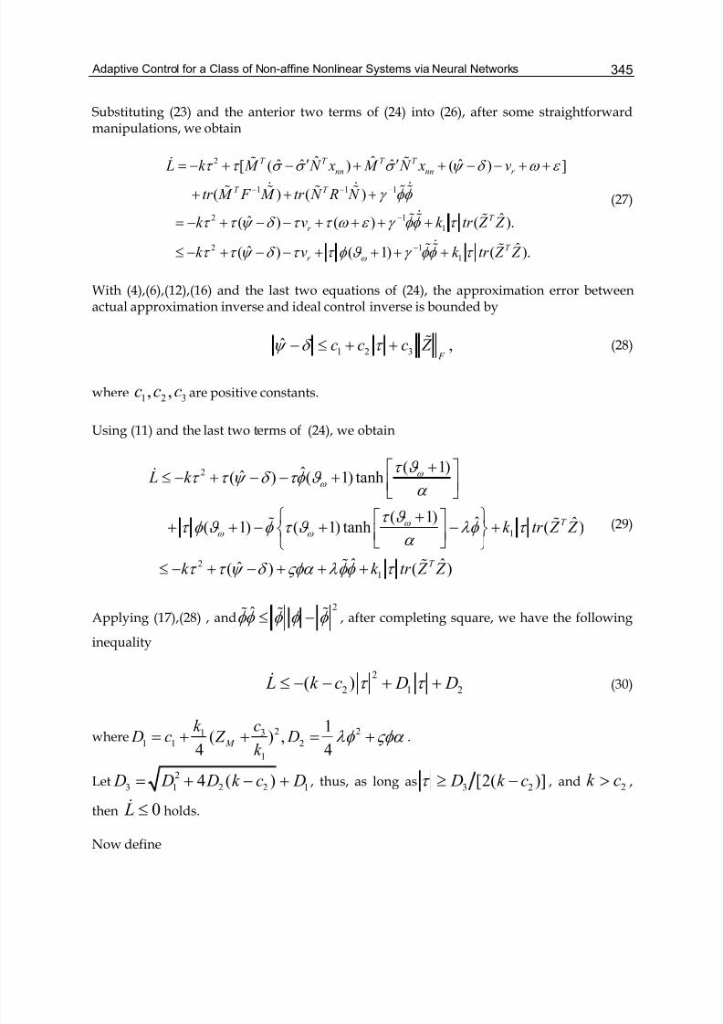
Adaptive Control for a Class of Non-affine Nonlinear Systems via Neural Networks 345
Substituting (23) and the anterior two terms of (24) into (26), after some straightforwardmanipulations, we obtain
2
1 1 1
2 1
1
2 1
1
ˆ ˆ ˆˆ ˆ ˆ[ ( ) ( ) ]
( ) ( )
ˆˆ( ) ( ) ( ).
ˆˆ( ) ( 1) ( ).
T T T T
nn nn r
T T
T
r
T
r
L k M N x M N x v
tr M F M tr N R N
k v k tr Z Z
k v k tr Z Z ω
τ τ σ σ σ ψ δ ω ε
γ φφ
τ τ ψ δ τ τ ω ε γ φφ τ
τ τ ψ δ τ τ φ ϑ γ φφ τ
− − −
−
−
′ ′= − + − + + − − + +
+ + +
= − + − − + + + +
≤ − + − − + + + +
& % %
&& & % %% % % %
&% % %
&% % %
(27)
With (4),(6),(12),(16) and the last two equations of (24), the approximation error betweenactual approximation inverse and ideal control inverse is bounded by
1 2 3ˆ ,
F c c c Z ψ δ τ − ≤ + + % (28)
where 1 2 3, ,c c c are positive constants.
Using (11) and the last two terms of (24), we obtain
2
1
2
1
( 1)ˆˆ( ) ( 1) tanh
( 1) ˆ ˆ( 1) ( 1) tanh ( )
ˆ ˆˆ( ) ( )
T
T
L k
k tr Z Z
k k tr Z Z
ω ω
ω ω ω
τ ϑ τ τ ψ δ τφ ϑ
α
τ ϑ τ φ ϑ φ τ ϑ λφ τ
α
τ τ ψ δ ςφα λφφ τ
+⎡ ⎤≤ − + − − + ⎢ ⎥⎣ ⎦
⎧ + ⎫⎡ ⎤+ + − + − +⎨ ⎬⎢ ⎥⎣ ⎦⎩ ⎭
≤ − + − + + +
&
% %
% %
(29)
Applying (17),(28) , and2
ˆφφ φ φ φ ≤ −% % % , after completing square, we have the following
inequality
2
2 1 2( ) L k c D Dτ τ ≤ − − + +& (30)
where 2 2311 1 2
1
1( ) ,
4 4 M
ck D c Z D
k λφ ςφα = + + = + .
Let2
3 1 2 2 14 ( ) D D D k c D= + − + , thus, as long as3 2[2( )] D k cτ ≥ − , and
2k c> ,
then 0 L ≤& holds.
Now define
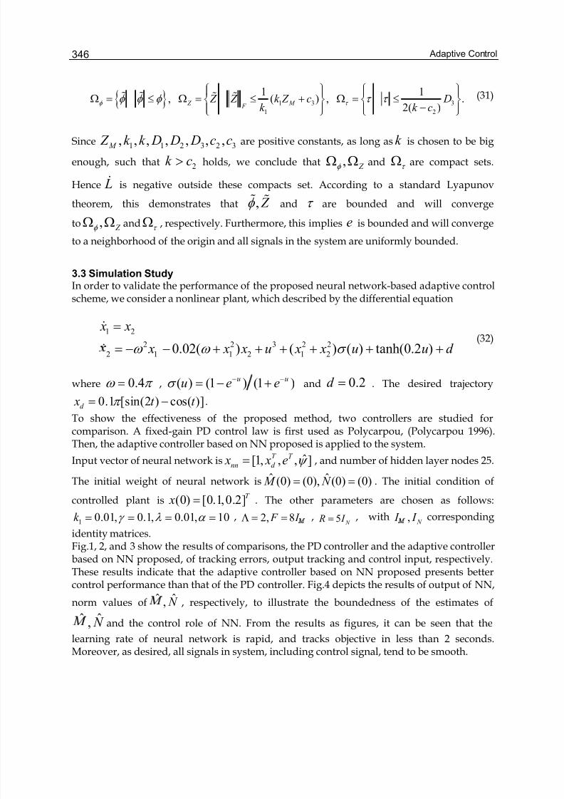
Adaptive Control346
1 3 3
1 2
1 1, ( ) , .
2( ) Z M
F Z Z k Z c D
k k cφ τ φ φ φ τ τ
⎧ ⎫ ⎧ ⎫⎪ ⎪ ⎪ ⎪Ω = ≤ Ω = ≤ + Ω = ≤⎨ ⎬ ⎨ ⎬
−⎪ ⎪ ⎪ ⎪⎩ ⎭ ⎩ ⎭
% % % % (31)
Since1 1 2 3 2 3, , , , , , , M Z k k D D D c c are positive constants, as long as k is chosen to be big
enough, such that 2k c> holds, we conclude that , Z φ Ω Ω and τ Ω are compact sets.
Hence L& is negative outside these compacts set. According to a standard Lyapunov
theorem, this demonstrates that , Z φ % % and τ are bounded and will converge
to , Z φ Ω Ω and τ Ω , respectively. Furthermore, this implies e is bounded and will converge
to a neighborhood of the origin and all signals in the system are uniformly bounded.
3.3 Simulation StudyIn order to validate the performance of the proposed neural network-based adaptive controlscheme, we consider a nonlinear plant, which described by the differential equation
1 2
2 2 3 2 2
2 1 1 2 1 20.02( ) ( ) ( ) tanh(0.2 )
x x
x x x u x x u u d ω ω σ
=
= − − + + + + + +
&
&(32)
where 0.4ω π = , ( ) (1 ) (1 )u uu e eσ − −= − + and 0.2d = . The desired trajectory
0.1 [sin(2 ) cos( )]d x t t π = − .
To show the effectiveness of the proposed method, two controllers are studied forcomparison. A fixed-gain PD control law is first used as Polycarpou, (Polycarpou 1996).Then, the adaptive controller based on NN proposed is applied to the system.
Input vector of neural network is ˆ[1, , , ]T T
nn d x x e ψ = , and number of hidden layer nodes 25.
The initial weight of neural network is ˆ ˆ(0) (0), (0) (0) M N = = . The initial condition of
controlled plant is (0) [0.1,0.2]T x = . The other parameters are chosen as follows:
1 0.01, 0.1, 0.01, 10k γ λ α = = = = , 2, 8 F I Λ = = , 5 N R I = , with , N I I corresponding
identity matrices.Fig.1, 2, and 3 show the results of comparisons, the PD controller and the adaptive controllerbased on NN proposed, of tracking errors, output tracking and control input, respectively.These results indicate that the adaptive controller based on NN proposed presents bettercontrol performance than that of the PD controller. Fig.4 depicts the results of output of NN,
norm values of ˆ ˆ, N , respectively, to illustrate the boundedness of the estimates of
ˆ ˆ, N and the control role of NN. From the results as figures, it can be seen that the
learning rate of neural network is rapid, and tracks objective in less than 2 seconds.Moreover, as desired, all signals in system, including control signal, tend to be smooth.
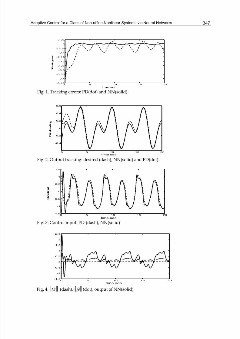
Adaptive Control for a Class of Non-affine Nonlinear Systems via Neural Networks 347
0 5 10 15 20-0.45
-0.4
-0.35
-0.3
-0.25
-0.2
-0.15
-0.1
-0.05
0
0.05
T r a c k i n g e r r o r
time sec
Fig. 1. Tracking errors: PD(dot) and NN(solid).
0 5 10 15 20
-0.4
-0.2
0
0.2
0.4
0.6
O u t p u t t r a c k i n g
time sec
Fig. 2. Output tracking: desired (dash), NN(solid) and PD(dot).
0 5 10 15 20-1.5
-1
-0.5
0
0.5
1
1.5
C o n t r o l i n p u t
time sec
Fig. 3. Control input: PD (dash), NN(solid)
0 5 10 15 20-1.5
-1
-0.5
0
0.5
1
1.5
2
2.5
time sec
Fig. 4. ˆ (dash), ˆ N (dot), output of NN(solid)
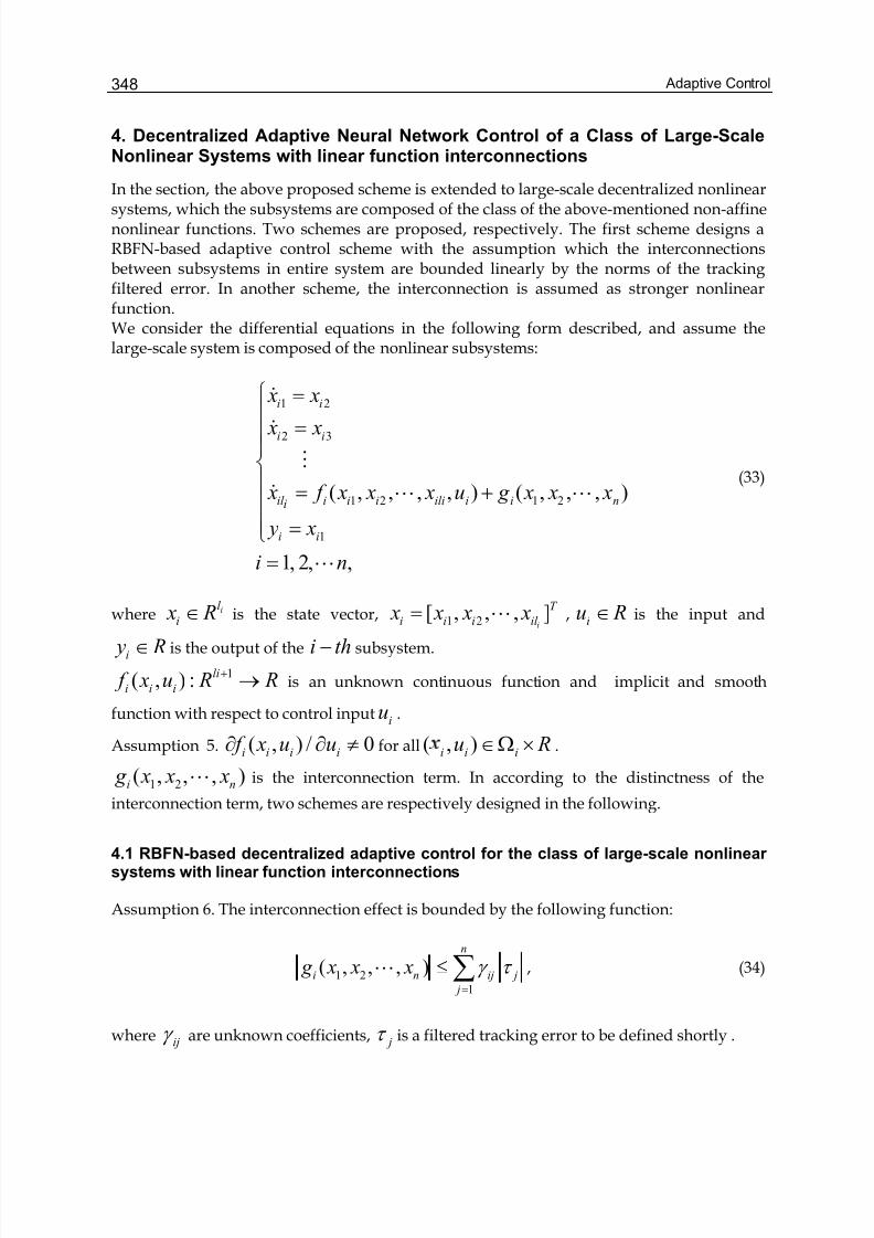
Adaptive Control348
4. Decentralized Adaptive Neural Network Control of a Class of Large-ScaleNonlinear Systems with linear function interconnections
In the section, the above proposed scheme is extended to large-scale decentralized nonlinearsystems, which the subsystems are composed of the class of the above-mentioned non-affinenonlinear functions. Two schemes are proposed, respectively. The first scheme designs aRBFN-based adaptive control scheme with the assumption which the interconnectionsbetween subsystems in entire system are bounded linearly by the norms of the trackingfiltered error. In another scheme, the interconnection is assumed as stronger nonlinearfunction.We consider the differential equations in the following form described, and assume thelarge-scale system is composed of the nonlinear subsystems:
1 2
2 3
1 2 1 2
1
( , , , , ) ( , , , )
1, 2, ,
i i
i i
il i i i ili i i n
i i
i
x x
x x
x f x x x u g x x x
y x
i n
⎧ =⎪
=⎪⎪⎨⎪ = +⎪⎪ =⎩
=
&
&
M
& L L
L
(33)
where il
i x R∈ is the state vector, 1 2[ , , , ]i
T
i i i il x x x x= L , iu R∈ is the input and
i y R∈ is the output of the i th− subsystem.
1( , ) : li
i i i f x u R R+ → is an unknown continuous function and implicit and smooth
function with respect to control inputi
u .
Assumption 5. ( , ) / 0i i i i f x u u∂ ∂ ≠ for all ( , )i i iu R∈Ω × .
1 2( , , , )i n g x x xL is the interconnection term. In according to the distinctness of the
interconnection term, two schemes are respectively designed in the following.
4.1 RBFN-based decentralized adaptive control for the class of large-scale nonlinear systems with linear function interconnections
Assumption 6. The interconnection effect is bounded by the following function:
1 2
1
( , , , )n
i n ij j
j
g x x x γ τ =
≤∑L , (34)
where ijγ are unknown coefficients, jτ is a filtered tracking error to be defined shortly .
Adaptive Control for a Class of Non-affine Nonlinear Systems via Neural Networks 349
The control objective is: determine a control law, force the output,i
y , to follow a given
desired output, di x , with an acceptable accuracy, while all signals involved must be
bounded.
Define the desired trajectory vector 1[ , , , ]il T
di di di di x y y y−= & L and ( ), , , i
T l
di di di di X y y y⎡ ⎤= ⎣ ⎦& L ,
tracking error 1 2[ , , , ]i
T
i i di i i il e x x e e e= − = L , thus, the filter tracking error can be
written as
( 2) ( 1)
,1 ,2 , 1[ 1] i i
i
l l T
i i i i i i i i l i ik e k e k e eτ − −
−= Λ = + + + +& Le , (35)
where the coefficients are chosen such that the polynomial( 2)
,1 ,2 , 1i
i
l
i i i l k k s k s−
−+ + +L
( 1)il s−+ is Hurwitz.
Assumption 7. The desired signal ( )di
t is bounded, so thatdi di X X ≤ , where di X is a
known constant.For an isolated subsystem, without interconnection function, by differentiating (35), thefiltered tracking error can be rewritten as
( )[0 ] ( , )i
l
l T
i il di i i i i i di x x e f x u Y τ = − + Λ = +& & (36)
with( )
[0 ]il T
di di i iY x e= − + Λ .
Define a continuous function
i i i dik Y δ τ = − − (37)
where ik is a positive constant. With Assumption 5, we know ( , ) 0i i i f x u u∂ ∂ ≠ ,
thus, [ ( , ) ] 0i i i i f x u uδ ∂ − ∂ ≠ . Considering the fact that 0i i
uδ ∂ ∂ = , we invoke the
implicit function theorem, there exists a continuous ideal control inputiu∗
in a
neighborhood of ( , )i i i x u R∈Ω × , such that ( , ) 0i i i f x u δ ∗ − = , i.e. ( , )i i i i f x uδ ∗= holds.
( , )i i i i f x uδ ∗= represents ideal control inverse.
Adding and subtractingiδ to the right-hand side of ( , )
il i i i ii x f x u g = +& of (33), one
obtains
( , )iil i i i i i i i di f x u g k Y δ τ = + − − −& , (38)
and yields
Adaptive Control350
( , )i i i i i i i ik f x u g τ τ δ = − + + −& . (39)
In the same the above-discussed manner as equations (9)-(10) , we can obtain the followingequation:
ˆ ˆ( , )i i i i f x uψ = . (40)
Based on the above conditions, in order to control the system and make it be stable, we
design the approximation pseudo-control input ˆiψ as follows:
ˆi i i di ci rik Y u vψ τ = − − + + , (41)
whereciu is output of a neural network controller, which adopts a RBFN,
riv is
robustifying control term designed in stability analysis.
Adding and subtracting ˆiψ to the right-hand side of (39), with ( , )i i i di i i ik Y f x uδ τ ∗= − − = ,
we have
ˆ( , , )i i i i i i i ci i i ri ik x u u u v g τ τ ψ δ ∗= − + Δ − + − − +%& , (42)
where ( , , ) ( , ) ( , )i i i i i i i i i i x u u f x u f x u∗ ∗Δ = −% is error between nonlinear function and its
ideal control function, we can use the RBFN to approximate it.
4.1.1 Neural network-based approximation
Given a multi-input-single-output RBFN, let 1in and 1im be node number of input layer and
hidden layer, respectively. The active function used in the RBFN is Gaussian
function,2 2
( ) exp[ 0.5( ) / ]l lk k iS z μ σ = − −x ,
11, , il n= ⋅ ⋅ ⋅ , 11, , ik m= ⋅ ⋅ ⋅ where 1 1in
i R z ×∈ is input
vector of the RBFN, 1 1i in m
i Rμ ×∈ and 1 1im
i Rσ ×∈ are the center matrix and the width vector.
Based on the approximation property of RBFN, ( , , )i i i i
u u ∗Δ% can be written as
( , , ) ( , , ) ( )T
i i i i i i i i i i iS x u u W z z μ σ ε ∗Δ = +% , (43)
where ( )i i z ε is approximation error of RBFN, 1 1im
iW R×∈ .
Assumption 8. The approximation error ( )nn xε is bounded by i Niε ε ≤ , with 0 Niε > is
an unknown constant.
The input of RBFN is chosen as ˆ[ , , ]T T
i i i i z x τ ψ = . Moreover, output of RBFN is designed as
Adaptive Control for a Class of Non-affine Nonlinear Systems via Neural Networks 351
ˆ ˆ ˆ( , , ).T
ci i i i i iS u W z μ σ = (44)
Define ˆ ˆ ˆ, ,i i iW μ σ as estimates of ideal , ,i i iW μ σ , which are given by the RBFN tuning
algorithms.
Assumption 9. The ideal values of , ,i i iW μ σ satisfy
, ,i iM i iM i iM F W W μ μ σ σ ≤ ≤ ≤ , (45)
where , ,iM iM iM
W μ σ are positive constants. F
⋅ and ⋅ denote Frobenius norm and 2-
norm, respectively. Define their estimation errors as
ˆ ˆ ˆ, , .i i i i i i i i iW W W μ μ μ σ σ σ = − = − = −% % % (46)
Using the notations: ˆ ˆ ˆ ˆ[ , , ], [ , , ], [ , , ]i i i i i i i i i i i i Z diag W Z diag W Z diag W σ μ σ μ σ = = =% % % % for
convenience.
The Taylor series expansion for a given iμ and iσ is
2ˆ ˆˆ ˆ( , , ) ( , , ) ( , )i i i i i i i i i i i i i iS S S S z z Oμ σ μ σ μ σ μ σ μ σ ′ ′= + + +% % % % (47)
where ˆ ˆˆ ˆ ˆ ˆ( , , ) , ( , , )i k i i i i i k i i i i
S S S z S z μ σ σ μ μ σ σ ′ ′∂ ∂ ∂ ∂ evaluated at ˆi iμ = ,
ˆi iσ σ = , 2( , )i iO σ % % denotes the terms of order two. We use notations: ˆ ˆ ˆ: ( , , ),i i i i iS S z σ =
: ( , , )i i i i i
S S z σ =% % % , : ( , , )i i i i iS S z μ σ = .
Following the procedure in Appendix B, it can be shown that the following operation. Thefunction approximation error can be written as
ˆ ˆ ˆ ˆˆ ˆˆ ˆˆ ˆ( ) ( ) ( ),T T T T
i i i i i i i i i i i i i i i iS S S S W S W S W S W t μ σ μ σ μ σ μ σ ω ′ ′ ′ ′− = − − + + +% % % (48)
The disturbance term ( )i t ω is given by
ˆ ˆ ˆ ˆˆ ˆˆ ˆ( ) ( ) ( ) ( )T T T
i i i i i i i i i i i i i iS S S S t W S S W W μ σ μ σ ω μ σ μ σ ′ ′ ′ ′= − + + − + (49)
Then, the upper bound of ( )i t ω can be written as
1
ˆ ˆ ˆ ˆˆ ˆˆ ˆ( ) ( ) 2T T
i i i i i i i i i i i i i i i F F F F F S S S S t W W W W μ σ μ σ ω ω ω μ σ μ σ ρ ϑ ′ ′ ′ ′≤ + + + + ≤ (50)
Adaptive Control352
where1
max( , , , 2 )i i i i i F
W W ω ρ μ σ = , ˆ ˆ ˆ ˆˆ ˆˆ ˆ 1T T
i i i i i i i i i F F F F
S S S S W W ω μ σ μ σ ϑ μ σ ′ ′ ′ ′= + + + + ,
with1
⋅ 1 norm. Notice thatiω ρ is an unknown coefficient, whereas
iω ϑ is a known
function.
4.1.2 Controller design and stability analysisSubstituting (43) and (44) into (42), we have
ˆˆ ˆ ( )T T
i i i i i i i i i ri i i ik W S W S v g z τ τ ψ δ ε = − + − + − − + +& , (51)
using (48), the above equation can become
ˆ ˆ ˆ ˆˆ ˆˆ ˆ( ) ( )
ˆ ( ) ( ).
T T
i i i i i i i i i i i i i i
i i ri i i i i
S S S S k W S W
v g z t
μ σ μ σ τ τ μ σ μ σ
ψ δ ε ω
′ ′ ′ ′= − + − − + +
+ − − + + +
%& % %(52)
Theorem 2. Consider the nonlinear subsystems represented by Eq. (33) and let assumptions
hold. If choose the pseudo-control input ˆiψ as Eq.(41), and use the following adaptation
laws and robust control law
ˆ ˆˆˆ ˆˆ ˆ( )i i i i i i i i Wi i iS S W F S W μ σ μ σ τ γ τ ′ ′⎡ ⎤= − − −⎣ ⎦&
, (53)
ˆ ˆˆ ˆT
i i i i i Wi i iS G W μ μ τ γ μ τ ′⎡ ⎤= −⎣ ⎦
& , (54)
ˆ ˆˆ ˆT
i i i i i Wi i iS H W σ σ τ γ σ τ ′⎡ ⎤= −⎣ ⎦& , (55)
**ˆ ˆtanh( )i i
i i i i i i i
i
ω φ ω φ
τ ϑ φ γ τ ϑ λ φ τ
α
⎡ ⎤= −⎢ ⎥
⎣ ⎦
&, (56)
2ˆ ˆ( )i di i di i id d γ τ λ τ = −&
, (57)
** ˆˆ tanh( )i i
ri i i i i
i
v d ω ω
τ ϑ φϑ τ
α = + , (58)
Adaptive Control for a Class of Non-affine Nonlinear Systems via Neural Networks 353
where* 1i iω ω ϑ ϑ = + , 0, 0, 0T T T
i i i i i i F F G G H H = > = > = > are any constant
matrices, , , , ,Wi i di i diφ φ γ γ γ λ λ andi
α are positive design parameters, ˆiφ is the estimated
value of the uncertain disturbance term max( , )i i Niω φ ρ ε = , defining ˆi i iφ φ φ = −% with
iφ % error, 0
id > is used to estimate unknown positive number to shield interconnection
effect, ˆi
d is its estimated value, with ˆi i i
d d d = −% estimated error, then, guarantee that all
signals in the system are bounded and the tracking errorie will converge to a neighborhood
of the origin.Proof. Consider the following positive define Lyapunov function candidate as
2 1 1 1 1 2 1 21 1( ) ( ) ( )
2 2
T T T
i i i i i i i i i i i i i di i L tr W F W tr G tr H d φ τ μ μ σ σ γ φ γ − − − − −⎡ ⎤= + + + + +⎣ ⎦%%% % % % % % (59)
The time derivative of the above equation is given by
1 1 1 1 1( ) ( ) ( )
T T T
i i i i i i i i i i i i i i i di i i L tr W F W tr G tr H d d φ τ τ μ μ σ σ γ φφ γ − − − − −= + + + + +
&&& % %& & % %& % %& % % % % (60)
Applying(52) to (60), we have
1 1 1 1 1
ˆ ˆ ˆ ˆˆ ˆˆ ˆ( ) ( )
ˆ
( ) ( ) ( )
T T
i i i i i i i i i i i i i
i i
i i ri i i i
T T T
i i i i i i i i i i i i di i i
S S S S k W S W L
v g
tr W F W tr G tr H d d
μ σ μ σ
φ
τ μ σ μ σ τ
ψ δ ε ω
μ μ σ σ γ φφ γ − − − − −
′ ′ ′ ′⎡ ⎤− + − − + += ⎢ ⎥
+ − − + + +⎢ ⎥⎣ ⎦
+ + + + +
% % %&
&&& % %& & % %% % % % % %
(61)
Substituting the adaptive laws (53), (54) and (55) into (61), and( ) ( )ˆ⋅ = − ⋅&&% ,yields
[ ] 1 1
2
1 1
2 *
ˆˆ ( )
ˆ( ) ( )
ˆ( )
ˆ( )
T
i i i i i i ri i i i Wi i i i i i i di i i
i i i i i ri i i i i i i Ni
T
Wi i i i i i i di i i
i i i i i ri i i i i i i
L k v g tr Z Z d d
k v g
tr Z Z d d
k v g
φ
ω ω
φ
ω
τ τ ψ δ ε ω γ τ γ φφ γ
τ τ ψ δ τ τ τ ρ ϑ ε
γ τ γ φφ γ
τ τ ψ δ τ τ τ φϑ
− −
− −
= − + − − + + + + + +
≤ − + − − + + +
+ + +
≤ − + − − + +
+
&& % %% %& %
&& % %% %%
1 1ˆ( )T
Wi i i i i i i di i itr Z Z d d φ γ τ γ φφ γ − −+ +
&& % %% %%
(62)
Adaptive Control354
Inserting (56) and (58) into the above inequality, we obtain*
2 * *
** 2
2
*2 * *
ˆˆ( ) tanh( )
ˆˆtanh( )
ˆ ˆ( ) ( )
ˆ( ) tanh( )
i ii i i i i i i i i i i i i i
i
i ii i i i i i i i
i
T
i i di i i Wi i i i
i ii i i i i i i i i i i i
i
L k g
d
d d tr Z Z
k
ω ω ω
ω ω φ
ω ω ω φ
τ ϑ τ τ ψ δ τ τ φϑ τ φϑ
α
τ ϑ φ τ ϑ λ φ τ τ
α
τ λ τ γ τ
τ ϑ τ τ ψ δ φ τ ϑ τ ϑ λ τ
α
≤ − + − + + −
⎡ ⎤− − −⎢ ⎥
⎣ ⎦
− − +
⎡ ⎤= − + − + − +⎢ ⎥
⎣ ⎦
&
%
% %
2
ˆ
ˆ ˆ( )
i i
T
i i i i di i i i Wi i i id g d d tr Z Z
φφ
τ τ λ τ γ τ − + + +
%
% %
(63)
Using (11), (63) becomes
2 2ˆ( )
ˆˆ ˆ( )
i i i i i i i i i i i i i
T
i i i i di i i Wi i i
L k d g
d d tr Z Z φ
τ τ ψ δ φς α τ τ
τ λ φφ λ γ
≤ − + − + − +
⎡ ⎤+ + +⎣ ⎦
&
%% %(64)
By completing square, we have
22 ˆ( )
4
ˆˆ ˆ( )
ii i i i i i i i i
i
T
i i i i di i i Wi i i
g L k
d
d d tr Z Z φ
τ τ ψ δ φ ς α
τ λ φ φ λ γ
≤ − + − + +
⎡ ⎤+ + +⎣ ⎦
&
%% %
(65)
With (41), (44), (53)-(58), approximation error between actual approximation inverse andideal control inverse is bounded by
1 2 3ˆ ,i i i i i i i
F c c c Z ψ δ τ − ≤ + + % (66)
where1 2 3, ,i i ic c c are positive constants.
( ) ( )2
2 1 3
2
ˆˆ ˆ( )4
i i i i i i i i i i i F
T ii i i i di i i Wi i i
i
L k c c c Z
g d d tr Z Z
d φ
τ τ φ ς α
τ λ φ φ λ γ
≤ − − + + +
⎡ ⎤+ + + +⎣ ⎦
& %
%% %
(67)
Since222
ˆˆ( ) , ,T
i i i i i i i i i i i i i i i F F F tr Z Z Z Z Z d d d d d φφ φ φ φ ≤ − ≤ − ≤ −
&% % % %% % %% % % hold, the
Adaptive Control for a Class of Non-affine Nonlinear Systems via Neural Networks 355
above inequality can be written as
( ) ( )2
2
2 1 3
22 2
4
( ) ( ) ( )
ii i i i i i i i i i i
F i
i i i i i di i i i Wi i i i F F F
g L k c c c Z
d
d d d Z Z Z φ
τ τ φ ς α
τ λ φ φ φ λ γ
≤ − − + + + +
⎡ ⎤+ − + − + −⎢ ⎥⎣ ⎦
& %
% %% % % %
(68)
By completing square for (68), we get
( )2
2
2 54
ii i i i i i i i i
i
L k c cd
τ τ φ ς α ≤ − − + + +& (69)
where 5 1 4i i ic c c= + ,with( )
2
2 2 3
44 4 4
Wi i ii F dii i i
Z cc d
φ γ λ λ
φ +
= + + .
For the overall system, it can be derived that the bound as
( )2
2
2 5
1 1 4
n ni
i i i i i i i i i
i i i
g L L k c c
d τ τ φ ς α
= =
⎧ ⎫= ≤ − − + + +⎨ ⎬
⎩ ⎭∑ ∑& & (70)
According to (34),
1
nT
i ij j i
j
g γ τ χ =
≤ = Γ∑ , define1 2[ , , ]T
n χ τ τ τ = L ,
1 2[ , , ]T
i i i inγ γ γ Γ = L ,1 21 2 22 2[ , , , ]n n K diag k c k c k c= − − −L ,
51 52 5[ , , , ]T
nC c c c= L
, ( )1
n
i i i
i
D φ ς α =
= ∑ , the above inequality can be rewritten as
2
min
1
4
( )
T T T T T
i i
i
L K C D E C Dd
E C D
χ χ χ χ χ χ
λ χ χ
⎛ ⎞≤ − − Γ Γ + + = − + +⎜ ⎟
⎝ ⎠
≤ − + +
&(71)
where1(4 ) T
i i i E K d −= − Γ Γ ,min ( ) E λ the minimum singular value of E . Then 0 L ≤& ,
as long as2i ik c> and sufficiently large
id , E would be positive definite, and
Adaptive Control356
( )
2
min
2
min min
3
( ),
4 ( ) 2 ( )
1, ,i i i i i Wi i i F F
Wi
C D E C A
E E
d d Z Z c
λ χ
λ λ
φ φ γ γ
+≥ + =
≥ ≥ ≥ +%% %
(72)
Now, we define
( )3
, ,
1,
i i i
d i i i Z i i Wi i i F F F Wi
i
i i
A
d d d Z Z Z c
χ φ χ χ φ φ φ
γ γ
Ω = ≤ Ω = ≤
⎧ ⎫⎪ ⎪Ω = ≤ Ω = ≤ +⎨ ⎬
⎪ ⎪⎩ ⎭
% %
% % % %(73)
Since3, , , ,i i i Wi i F
Z d cφ γ are positive constants, we conclude that χ Ω , Z iΩ ,
iφ Ω
and d iΩ are compact sets. Hence L& is negative outside these compacts set. According to a
standard Lyapunov theorem, this demonstrates that , ,i i i Z d φ %%% and χ are bounded and will
converge to χ Ω ,
Z iΩ ,iφ
Ω andd i
Ω , respectively. Furthermore, this impliesi
e is bounded
and will converge to a neighborhood of the origin and all signals in the system are bounded.
4.1.3 Simulation StudyIn order to validate the effectiveness of the proposed scheme, we implement an example,and assume that the large-scale system is composed of the following two subsystemsdefined by
11 12
2 2
12 11 11 12 1
2 2
11 12 1 21
1: 0.02( )
( ) ( ) 0.2 sin(0.2 )
Subsystem
x x
x x x x u
x u x
ω ω
σ
=⎧⎪
= − + − +⎨⎪
+ + + +⎩
&
& (74)
21 22
2 2
22 21 22 2 2
3
2 11
2 : 0.1(1 ) tanh(0.1 )
0.15 tanh(0.1 )
Subsystem
x x
x x u u
u x
=⎧⎪
= + + +⎨⎪
+ +⎩
&
& (75)
where 0.4ω π = , 1 1
1( ) (1 ) (1 )u u
u e eσ − −= − + . The desired trajectory11 0.1 [sin(2 ) cos( )]d x t t π = − ,
21 0.1 cos(2 )d t π = .
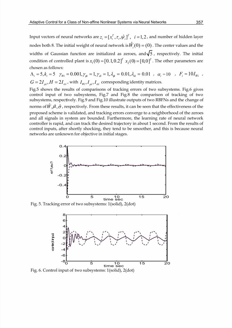
Adaptive Control for a Class of Non-affine Nonlinear Systems via Neural Networks 357
Input vectors of neural networks are ˆ[ , , ] , 1,2T T
i i i i z x iτ ψ = = , and number of hidden layer
nodes both 8. The initial weight of neural network is ˆ (0) (0)iW = . The center values and the
widths of Gaussian function are initialized as zeroes, and 5 , respectively. The initial
condition of controlled plant is1(0) [0.1,0.2]T x =
2 (0) [0,0]T x = . The other parameters are
chosen as follows:
5, 5i ik Λ = = 0.001, 1, 1, 0.01, 0.01Wi i di i diφ φ γ γ γ λ λ = = = = = , 10iα = , 10i Wi F I = ,
2 , 2i iG I H I μ σ = = , with , ,Wi i i I I I μ σ corresponding identity matrices.
Fig.5 shows the results of comparisons of tracking errors of two subsystems. Fig.6 givescontrol input of two subsystems, Fig.7 and Fig.8 the comparison of tracking of twosubsystems, respectively. Fig.9 and Fig.10 illustrate outputs of two RBFNs and the change of
norms of ˆ ˆ ˆ, ,W σ , respectively. From these results, it can be seen that the effectiveness of the
proposed scheme is validated, and tracking errors converge to a neighborhood of the zeroesand all signals in system are bounded. Furthermore, the learning rate of neural networkcontroller is rapid, and can track the desired trajectory in about 1 second. From the results ofcontrol inputs, after shortly shocking, they tend to be smoother, and this is because neuralnetworks are unknown for objective in initial stages.
0 5 10 15 20
-0.4
-0.2
0
0.2
0.4
e
, e
time sec
Fig. 5. Tracking error of two subsystems: 1(solid), 2(dot)
0 5 10 15 20-8
-6
-4
-2
0
2
4
6
8
c o n t r o
l i n p u t
time sec
Fig. 6. Control input of two subsystems: 1(solid), 2(dot)
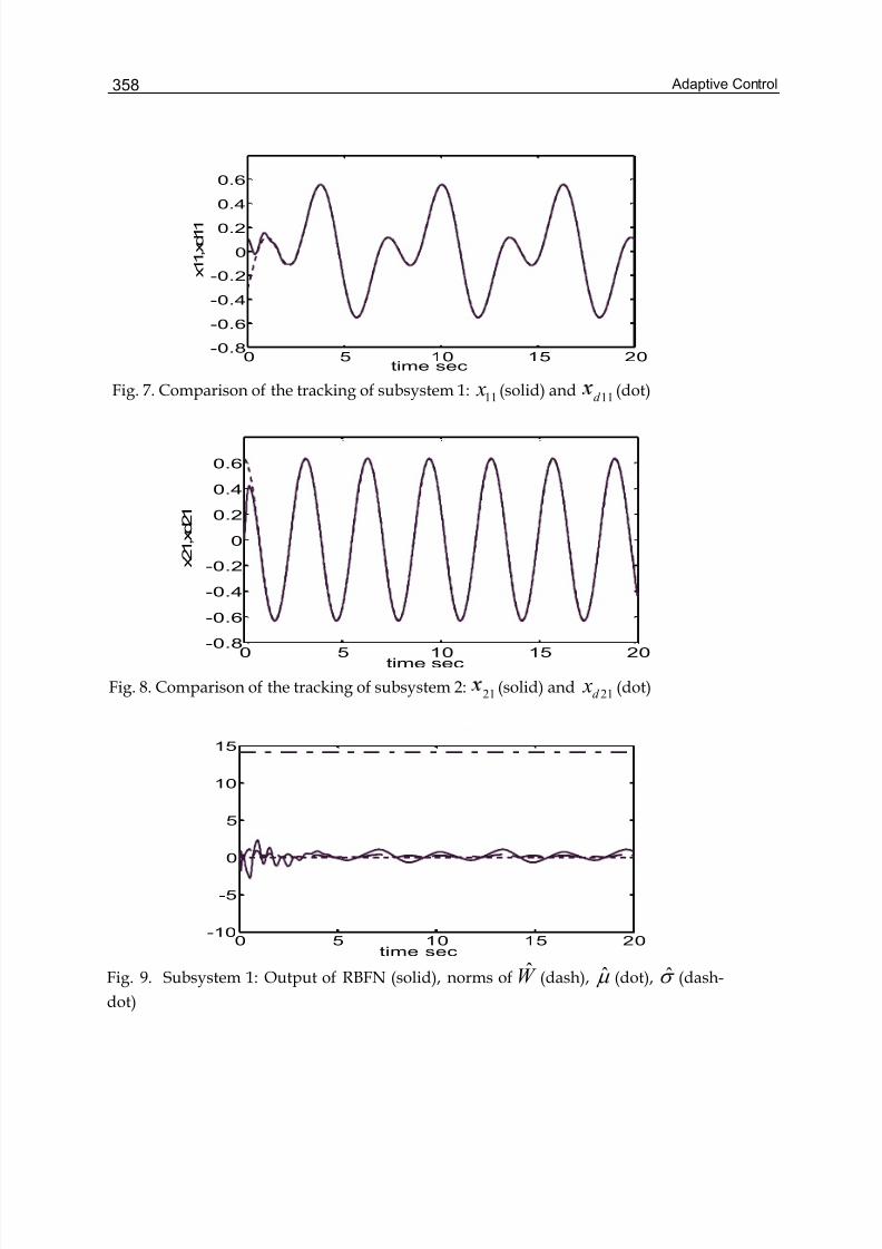
Adaptive Control358
0 5 10 15 20-0.8
-0.6
-0.4
-0.2
0
0.2
0.4
0.6
x 1 1 , x
d 1 1
time sec
Fig. 7. Comparison of the tracking of subsystem 1:11 x (solid) and
11d (dot)
0 5 10 15 20-0.8
-0.6
-0.4
-0.2
0
0.2
0.4
0.6
x 2 1 , x
d 2 1
time sec
Fig. 8. Comparison of the tracking of subsystem 2: 21 (solid) and 21d x (dot)
0 5 10 15 20-10
-5
0
5
10
15
time sec
Fig. 9. Subsystem 1: Output of RBFN (solid), norms of W (dash), μ (dot), σ (dash-
dot)
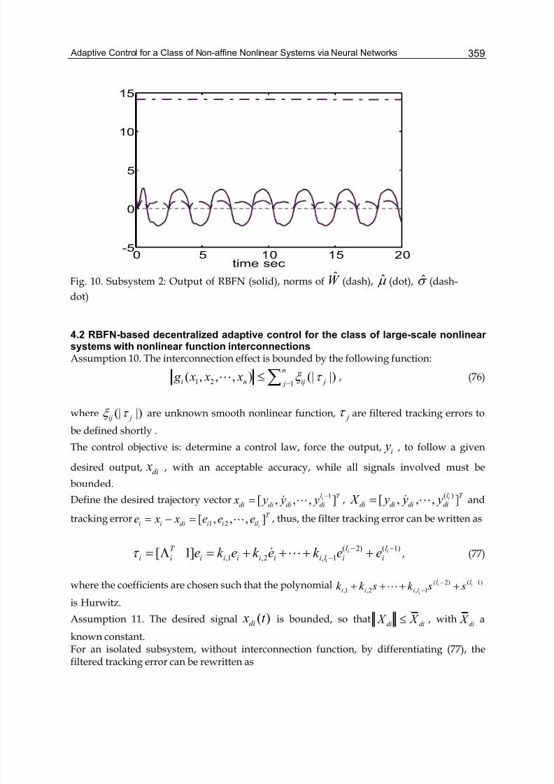
Adaptive Control for a Class of Non-affine Nonlinear Systems via Neural Networks 359
4.2 RBFN-based decentralized adaptive control for the class of large-scale nonlinear systems with nonlinear function interconnectionsAssumption 10. The interconnection effect is bounded by the following function:
1 2 1( , , , ) (| |)
n
i n ij j j g x x x ξ τ
=≤∑L , (76)
where (| |)ij jξ τ are unknown smooth nonlinear function, jτ are filtered tracking errors to
be defined shortly .
The control objective is: determine a control law, force the output, i y , to follow a given
desired output,di
x , with an acceptable accuracy, while all signals involved must be
bounded.
Define the desired trajectory vector 1[ , , , ]il T
di di di di x y y y−= & L ,
( )[ , , , ]il T
di di di di X y y y= & L and
tracking error1 2[ , , , ]
i
T
i i di i i il e x x e e e= − = L , thus, the filter tracking error can be written as
( 2) ( 1)
,1 ,2 , 1[ 1] i i
i
l l T
i i i i i i i i l i ie k e k e k e eτ − −
−= Λ = + + + +& L , (77)
where the coefficients are chosen such that the polynomial ( 2) ( 1)
,1 ,2 , 1i i
i
l l
i i i l k k s k s s− −
−+ + + +L
is Hurwitz.
Assumption 11. The desired signal ( )di x t is bounded, so thatdi di X X ≤ , with
di X a
known constant.For an isolated subsystem, without interconnection function, by differentiating (77), thefiltered tracking error can be rewritten as
0 5 10 15 20-5
0
5
10
15
time sec
Fig. 10. Subsystem 2: Output of RBFN (solid), norms of W (dash), μ (dot), σ (dash-
dot)
Adaptive Control360
( )[0 ] ( , )i
l
l T
i il di i i i i i di y e f x u Y τ = − + Λ = +& & , (78)
with( )
[0 ]il T
di di i iY y e= − + Λ .
Define a continuous function
i i i dik Y δ τ = + , (79)
where ik is a positive constant. With Assumption 5, we know ( , ) 0i i i f x u u∂ ∂ ≠ ,
thus, [ ( , ) ] 0i i i i
f x u uδ ∂ − ∂ ≠ . Considering the fact that 0i i
uδ ∂ ∂ = , with the implicit
function theorem, there exists a continuous ideal control input iu∗in a neighborhood
of ( , )i i iu R∈Ω × , such that ( , ) 0i i i f x u δ ∗ − = , i.e. ( , )i i i i f x uδ ∗= holds.
Here, ( , )i i i i f x uδ ∗= represents an ideal control inverse. Adding and subtractingiδ to the
right-hand side of ( , )il i i i ii x f x u g = +& of (33), one obtains
( , )il i i i i i di i ii x f x u g Y k δ τ = + + − −& , (80)
and yields
( , )i i i i i i i ik f x u g τ τ δ = − + + +& , (81)
Similar to the above-mentioned equation (40), ˆ ˆ( , )i i i i f x uψ = holds.
Based on the above conditions, in order to control the system and make it be stable, we
design the approximation pseudo-control input ˆiψ as follows:
ˆˆ (| |)T
i i i di ci gi gi i i rik Y u W S vψ τ τ τ = − − − − − , (82)
whereci
u is output of a neural network controller, which adopts a RBFN,ri
v is
robustifying control term designed in stability analysis, ˆ (| |)T
gi gi iW S τ is used to
compensate the interconnection nonlinearity (we will define later).
Adding and subtracting ˆi
ψ to the right-hand side of (81), with ( , )i i i di i i i
k Y f x uδ τ ∗= + = ,
we have
ˆ ˆ( , , ) (| |)T
i i i i i i i ci gi gi i i i i ri ik x u u u W S v g τ τ τ τ δ ψ ∗= − + Δ − − + − − +%& , (83)
Adaptive Control for a Class of Non-affine Nonlinear Systems via Neural Networks 361
where ( , , ) ( , ) ( , )i i i i i i i i i i
u u f x u f x u∗ ∗Δ = −% is error between the nonlinear function
and its ideal control function, we can use the RBFN to approximate it.
4.2.1 Neural network-based approximation
Based on the approximation property of RBFN, ( , , )i i i i x u u ∗Δ% can be written as
( , , ) ( ) ( )T
i i i i i i i i iS x u u W z z ε ∗Δ = +% , (84)
wherei
W is the weight vector, ( )i i
S z is Gaussian basis function, ( )i i z ε is the
approximation error and the input vectorq
i z R∈ , q the number of input node.
Assumption 12. The approximation error ( )i i z ε is bounded by | |i Niε ε ≤ , with 0 Niε > is
an unknown constant. The input of the RBFN is chosen as ˆ[ , , ]T T
i i i i z x τ ψ = . Moreover,
output of the RBFN is designed as
ˆ ( ).T
ci i i iS u W z = (85)
Define ˆi
W as estimates of ideali
W , which are given by the RBFN tuning algorithms.
Assumption 13. The ideal value of iW satisfies
|| ||i iM W W ≤ , (86)
whereiM W is positive known constant, with estimation errors as ˆ
i i iW W W = −% .
4.2.2 Controller design and stability analysisSubstituting (84) and (85) into (83), we have
ˆˆ (| |) ( )T T
i i i i i i i ri i gi gi i i i ik W S v g W S z τ τ δ ψ τ τ ε = − + + − − + − +%& (87)
Theorem 3. Consider the nonlinear subsystems represented by Eq. (33) and let assumptions
hold. If choose the pseudo-control input ˆi
ψ as Eq.(82), and use the following adaptation
laws and robust control law
ˆ ˆ[ | |]i i i i Wi i iW F S W τ γ τ = −&
, (88)
Adaptive Control362
2ˆ ˆ[ (| |) | |] gi i gi i i gi gi iW G S W τ τ γ τ = −&
, (89)
ˆ ˆ[ (| | 1) tanh( ) | |]i i i i i i i i iφ φ φ λ τ τ τ α γ φ τ = + −&
, (90)
ˆ (| | 1) tanh( )ri i i i iv φ τ τ α = + , (91)
where 0T
i i F F = > , 0T
i iG G= > are any constant matrices, , , ,i Wi gi iφ φ λ γ γ γ andiα are
positive design parameters, ˆiφ is the estimated value of the unknown approximation errors,
which will be defined shortly, then, guarantee that all signals in the system are bounded and
the tracking errori
e will converge to a neighborhood of the origin.
Proof. Consider the following positive define Lyapunov function candidate as
2 1 1 1 22 T T
i i i i i gi i gi i i L W F W W G W φ τ λ φ − − −= + + + %% % % % (92)
The time derivative of the above equation is given by
1 1 1T T
i i i i i i gi i gi i i i L W F W W G W φ τ τ λ φφ − − −= + + +&& % %& % % % %& (93)
Applying (87) and(53) to (59) and( ) ( )ˆ⋅ = − ⋅&&% , we have
1 1
ˆˆ[ (| |) ]
ˆ | |
T
i i i i i i ri i gi gi i i i
T T
Wi i i i gi i gi i i i
L k v g W S
W W W G W φ
τ τ δ ψ τ τ ε
γ τ λ φφ − −
= − + − − + − +
+ + +
&
&& % %% % %(94)
Using (76), (94) is rewritten as
2
1
1 1
ˆˆ( ) [ (| |) (| |) ]
ˆ| |
n T
i i i i i i ri i i ij j gi gi i i j
T T
i Ni i i i Wi i i i gi i gi
L k v W S
W W W G W φ
τ τ δ ψ τ τ ξ τ τ τ
τ ε λ φφ γ τ
=
− −
≤ − + − − + −
+ + + +
∑&
& &% % % % %
(95)
Since ( )ijξ ⋅ is a smooth function, there exists a smooth function (| |)ij jζ τ , (1 , )i j n≤ ≤
such that (| |) | | (| |)ij j j ij jξ τ τ ζ τ = hold. Thus, we have
Adaptive Control for a Class of Non-affine Nonlinear Systems via Neural Networks 363
2 2
1
1 1
ˆˆ( ) [ (| |) (| |)]
ˆ| | | |
n T
i i i i i i ri i i ij j gi gi i j
T T
i Ni i i i Wi i i i gi i gi
L k v W S
W W W G W φ
τ τ δ ψ τ τ ζ τ τ
τ ε λ φφ γ τ
=
− −
≤ − + − − + −
+ + + +
∑&
& &% % % % %
(96)
Since the function1
(| |) (| |)n
i i ij iid τ ζ τ
== ∑ is smooth and
iτ is on a compact set,
(| |)i i
d τ can be approximated via a RBFN, i.e., (| |) (| |)T
i i gi gi i gid W S τ τ ε = + , with
bounded approximation error giε , | | gi gNiε ε ≤ . ˆ giW is estimate of ideal giW , with
boundedness || || gi gMiW W ≤ , 0 gMiW > a known constant, and the estimation errors as
ˆ gi gi giW W W = −% . Then, (96) becomes
2
1
1 1
2 2 2
1 1
ˆˆ( ) [ ( ) ( ) ]
ˆ
ˆ( ) (| |) | |
ˆ
nT
i i i i i i ri i i ij j gi gi i i
j
T T
i Ni i i i Wi i i i gi i gi
T
i i i i i ri i i gi gi i gi i i Ni
T T
i i i Wi i i i gi i
L k v W S
W W W G W
k v W S
W W W G
φ
φ
τ τ δ ψ τ τ ξ τ τ τ
τ ε λ φφ γ τ
τ τ δ ψ τ τ τ ε τ τ ε
λ φφ γ τ
=
− −
− −
≤ − + − − + −
+ + + +
≤ − + − − + + +
+ + +
∑&
& &% % % % %
%
&% % % % % gi
W &
(97)
Substituting the adaptive law (89), we obtain
2 2 1ˆ( ) | |
ˆ ˆ| | | |
i i i i i i ri i gNi i i Ni i i i
T T
Wi i i i gi gi gi i
L k v
W W W W
φ τ τ δ ψ τ ε τ τ ε λ φφ
γ τ γ τ
−≤ − + − − + + +
+ +
&% %&
% %(98)
Define max( , )i Ni gNiφ ε ε = , with ˆ
iφ is its estimate, and ˆi i iφ φ φ = −% with
iφ % error. (98) can
be rewritten as
2 2
1
ˆ( ) ( )
ˆ ˆ
i i i i i i ri i i i i
T T
i i i Wi i i i gi gi gi i
L k v
W W W W φ
τ τ δ ψ τ φ τ τ
λ φφ γ τ γ τ −
≤ − + − − + +
+ + +
&
&% % % %(99)
Applying the adaptive law (56) and robust control term (58), we have
Adaptive Control364
2
2
ˆˆ( ) ( 1) tanh( ) ( 1)
ˆˆ ˆ( 1) tanh( )
ˆ( ) ( 1) ( 1) tanh( )
ˆ ˆ
i i i i i i i i i i i i i i
T T
i i i i i Wi i i i gi gi gi i i i i i
i i i i i i i i i i i i i
T T
Wi i i i gi gi gi i i
L k
W W W W
k
W W W W
φ
φ
τ τ δ ψ φτ τ τ α φ τ τ
φτ τ τ α γ τ γ τ λ φφ τ
τ τ δ ψ φ τ τ φτ τ τ α
γ τ γ τ λ φ
≤ − + − − + + +
− + + + +
= − + − + + − +
+ + +
&
% %% %
%% %
2
ˆ
ˆ( ) ( 1) tanh( )
ˆˆ ˆ
i i i
i i i i i i i i i i i
T T
Wi i i i gi gi gi i i i i i
k
W W W W φ
φ τ
τ τ δ ψ φ τ τ τ τ α
γ τ γ τ λ φφ τ
= − + − + + ⎡ − ⎤⎣ ⎦
+ + + %% %
(100)
Using (11), we get
2 ˆ( ) (| | 1)
ˆˆ ˆ| | | | | |
i i i i i i i i i
T T
Wi i i i gi gi gi i i i i i
L k
W W W W φ
τ τ δ ψ φ τ ςα
γ τ γ τ γ φφ τ
≤ − + − + +
+ + +
&
%% %(101)
With (82), (85), and (88)-(91), the approximation error between the ideal control inverse and
the actual approximation inverse is bounded by1 2
ˆ| | | |i i i i ic cδ ψ τ − ≤ +
3 4|| || || ||,i i i gic W c W + +% % with 1 2 3 4, , ,i i i ic c c c positive constants. Moreover, we utility the
facts,2ˆ || |||| || || ||T a a a a a≤ −% % % , (101) can be rewritten as
( ) ( )
( )
2
2 1 3 4
2
3
22
2 1 4
2
( )
( )
( )
( )
( )
Wi i i i
i i i i i i i i i gi i gi gi gi gi i i i
i i i i
Wi i i i i
i i i i i i i i i gi gi gi i gi
i i i
W W W
L k c c c W c W W W W
W W c W
k c c W W c W
φ
φ
γ
τ τ τ γ φς α
λ φ φ φ
γ
τ τ φς α τ γ
λ φ φ φ
⎡ ⎤−⎢ ⎥⎢ ⎥≤ − − + + + + + − +⎢ ⎥⎢ ⎥+ −⎣ ⎦
⎡ ⎤− + +⎢ ⎥⎣ ⎦
⎡ ⎤≤ − − + + + + − + +⎢ ⎥⎣ ⎦
− +
% %
& % % % %
% %
% %
% %
% %i
⎧ ⎫⎪ ⎪⎪ ⎪⎪ ⎪⎨ ⎬⎪ ⎪⎪ ⎪⎪ ⎪⎩ ⎭
(102)
Completing square for (102), we have
( ) 2
2 8 | |i i i i i i i i i L k c cτ τ φ ς α ≤ − − + +& (103)
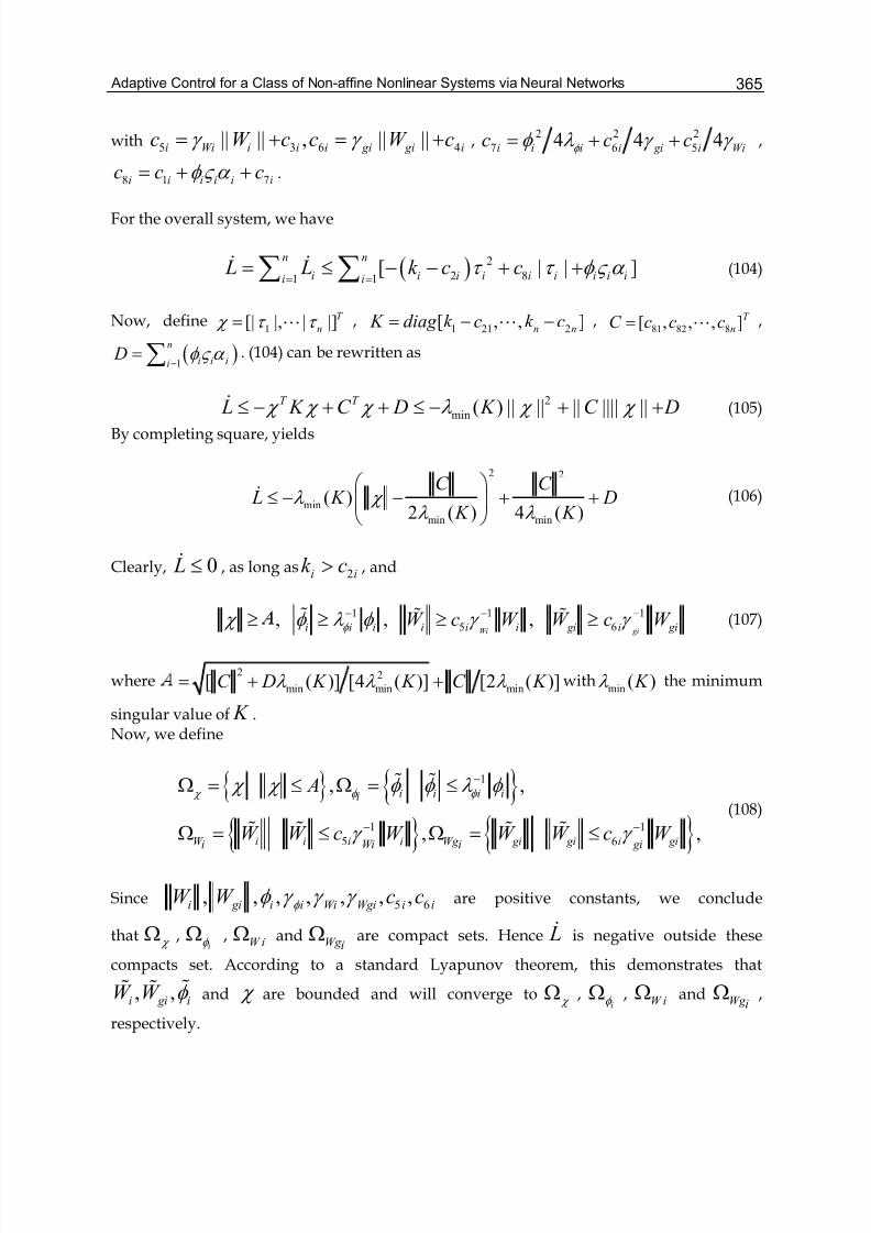
Adaptive Control for a Class of Non-affine Nonlinear Systems via Neural Networks 365
with5 3 6 4|| || , || ||i Wi i i i gi gi ic W c c W cγ γ = + = + ,
2 2 2
7 6 54 4 4i i i i gi i Wic c cφ φ λ γ γ = + + ,
8 1 7i i i i i ic c cφς α = + + .
For the overall system, we have
( ) 2
2 81 1[ | | ]
n n
i i i i i i i i ii i L L k c cτ τ φ ς α
= == ≤ − − + +∑ ∑& & (104)
Now, define1[| |, | |]T
n χ τ τ = L ,1 21 2
[ , , ]n n
K diag k c k c= − −L ,81 82 8[ , , , ]T
nC c c c= L ,
( )1
n
i i ii D φς α
== ∑ . (104) can be rewritten as
2
min ( ) || || || |||| ||T T L K C D K C D χ χ χ λ χ χ ≤ − + + ≤ − + +& (105)
By completing square, yields
2 2
min
min min
( )2 ( ) 4 ( )
C C L K D
K K λ χ
λ λ
⎛ ⎞≤ − − + +⎜ ⎟
⎝ ⎠
& (106)
Clearly, 0 L ≤& , as long as2i ik c> , and
1 1 1
5 6, , ,Wi gii i i i i i gi i gi
W c W W c W φ χ φ λ φ γ γ − − −≥ ≥ ≥ ≥% % % (107)
where2 2
min min min[ ( )] [4 ( )] [2 ( )]C D K K C K λ λ λ = + + withmin ( ) K λ the minimum
singular value of K .Now, we define
1
1 1
5 6
, ,
, ,
i i i i
W i i i i Wg gi gi i gi
i
i Wi i gi
A
W W c W W W c W
χ φ φ χ χ φ φ λ φ
γ γ
−
− −
Ω = ≤ Ω = ≤
Ω = ≤ Ω = ≤
% %
% % % %(108)
Since 5 6, , , , , , ,i gi i i Wi Wgi i iW W c cφ φ γ γ γ are positive constants, we conclude
that χ Ω ,iφ
Ω , W iΩ and Wg iΩ are compact sets. Hence L& is negative outside these
compacts set. According to a standard Lyapunov theorem, this demonstrates that
, ,i gi iW W φ %% % and χ are bounded and will converge to χ Ω ,
iφ Ω , W iΩ and Wg i
Ω ,
respectively.
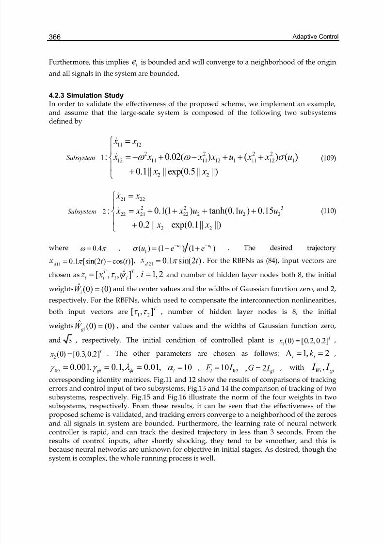
Adaptive Control366
Furthermore, this impliesi
e is bounded and will converge to a neighborhood of the origin
and all signals in the system are bounded.
4.2.3 Simulation StudyIn order to validate the effectiveness of the proposed scheme, we implement an example,and assume that the large-scale system is composed of the following two subsystemsdefined by
11 12
2 2 2 2
12 11 11 12 1 11 12 1
2 2
1: 0.02( ) ( ) ( )
0.1|| || exp(0.5 || ||)
Subsystem
x x
x x x x u x x u
x x
ω ω σ
=⎧⎪
= − + − + + +⎨⎪ +⎩
&
& (109)
21 22
2 2 3
22 21 22 2 2 2
2 2
2 : 0.1(1 ) tanh(0.1 ) 0.15
0.2 || || exp(0.1|| ||)
Subsystem
x x
x x x u u u
x x
=⎧⎪
= + + + +⎨⎪ +⎩
&
& (110)
where 0.4ω π = , 1 1
1( ) (1 ) (1 )u u
u e eσ − −= − + . The desired trajectory
11 0.1 [sin(2 ) cos( )]d t t π = − ,21 0.1 sin(2 )d t π = . For the RBFNs as (84), input vectors are
chosen as ˆ[ , , ]T T
i i i i z x τ ψ = , 1,2i = and number of hidden layer nodes both 8, the initial
weights ˆ (0) (0)iW = and the center values and the widths of Gaussian function zero, and 2,
respectively. For the RBFNs, which used to compensate the interconnection nonlinearities,
both input vectors are1 2
[ , ]T τ τ , number of hidden layer nodes is 8, the initial
weights ˆ (0) (0) giW = , and the center values and the widths of Gaussian function zero,
and 5 , respectively. The initial condition of controlled plant is1(0) [0.2,0.2]T x = ,
2 (0) [0.3,0.2]T x = . The other parameters are chosen as follows: 1, 2i ik Λ = = ,
0.001, 0.1, 0.01,Wi i iφ φ γ γ λ = = = 10i
α = , 10i Wi F I = , 2 giG I = , with ,Wi gi I I
corresponding identity matrices. Fig.11 and 12 show the results of comparisons of trackingerrors and control input of two subsystems, Fig.13 and 14 the comparison of tracking of twosubsystems, respectively. Fig.15 and Fig.16 illustrate the norm of the four weights in twosubsystems, respectively. From these results, it can be seen that the effectiveness of theproposed scheme is validated, and tracking errors converge to a neighborhood of the zeroesand all signals in system are bounded. Furthermore, the learning rate of neural networkcontroller is rapid, and can track the desired trajectory in less than 3 seconds. From theresults of control inputs, after shortly shocking, they tend to be smoother, and this isbecause neural networks are unknown for objective in initial stages. As desired, though thesystem is complex, the whole running process is well.
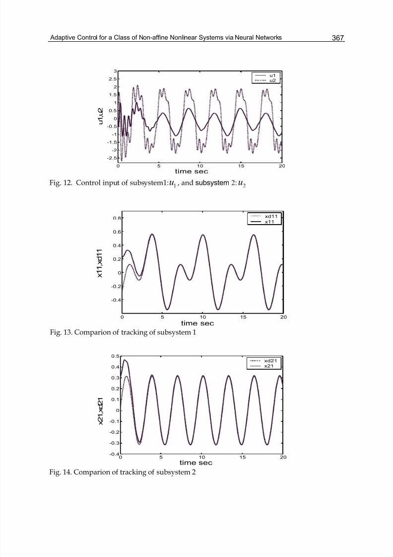
Adaptive Control for a Class of Non-affine Nonlinear Systems via Neural Networks 367
0 5 10 15 20
-2.5
-2
-1.5
-1
-0.5
0
0.5
1
1.5
2
2.5
3u1u2
u 1
, u 2
time sec
Fig. 12. Control input of subsystem1: 1u , and subsystem 2: 2u
0 5 10 15 20
-0.4
-0.2
0
0.2
0.4
0.6
0.8 xd11
x11
x 1 1
, x d 1 1
time sec
Fig. 13. Comparion of tracking of subsystem 1
0 5 10 15 20-0.4
-0.3
-0.2
-0.1
0
0.1
0.2
0.3
0.4
0.5xd21x21
x 2 1 , x
d 2 1
time sec
Fig. 14. Comparion of tracking of subsystem 2
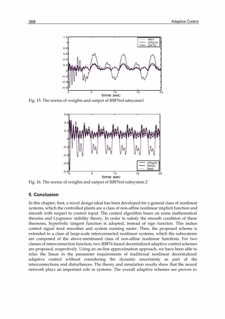
Adaptive Control368
0 5 10 15 20
-0.6
-0.4
-0.2
0
0.2
0.4
0.6
0.8
1
1.2NN1||Wg1||||W1||
time sec
Fig. 15. The norms of weights and output of RBFNof subsystem1
0 5 10 15 20-0.8
-0.6
-0.4
-0.2
0
0.2
0.4
0.6
||Wg2||||W2||
NN2
time sec
Fig. 16. The norms of weights and output of RBFNof subsystem 2
5. Conclusion
In this chapter, first, a novel design ideal has been developed for a general class of nonlinearsystems, which the controlled plants are a class of non-affine nonlinear implicit function andsmooth with respect to control input. The control algorithm bases on some mathematicaltheories and Lyapunov stability theory. In order to satisfy the smooth condition of thesetheorems, hyperbolic tangent function is adopted, instead of sign function. This makescontrol signal tend smoother and system running easier. Then, the proposed scheme isextended to a class of large-scale interconnected nonlinear systems, which the subsystemsare composed of the above-mentioned class of non-affine nonlinear functions. For twoclasses of interconnection function, two RBFN-based decentralized adaptive control schemesare proposed, respectively. Using an on-line approximation approach, we have been able torelax the linear in the parameter requirements of traditional nonlinear decentralizedadaptive control without considering the dynamic uncertainty as part of theinterconnections and disturbances. The theory and simulation results show that the neuralnetwork plays an important role in systems. The overall adaptive schemes are proven to
Adaptive Control for a Class of Non-affine Nonlinear Systems via Neural Networks 369
guarantee uniform boundedness in the Lyapunov sense. The effectiveness of the proposedcontrol schemes are illustrated through simulations. As desired, all signals in systems,including control signals, are tend to smooth.
6. Acknowledgments
This research is supported by the research fund granted by the Natural Science Foundationof Shandong (Y2007G06) and the Doctoral Foundation of Qingdao University of Science andTechnology.
7. References
Lewis,F.L.; Yesildirek A. & Liu K.(1996). Multilayer neural-net robot controller withguaranteed tracking performance. IEEE Trans.on Neural Networks, Vol. 7, No.2, Mar.1996, pp.388-399, ISSN 1045-9227
Yu, W. & Li, X.(2002). Adaptive control with multiple neural networks. Proceeding of the American Control Conference, pp. 1543-1549, ISBN 0-7803-7298-0, May 8-10,2002Anchorage, AK
Yesidirek, A. and Lewis,F.L.(1995). Feedback linearization using neural networks. Automatica, Vol.31, No.11, 1995, pp. 1659-1664, ISSN 0005-1098
Calise,A.J. & Hovakimyan, N. (2001). Adaptive output feedback control of nonlinear systemusing neural networks. Automatica, Vol.37, 2001, pp.1201-1211, ISSN 0005-1098
Ge, S. S. ; Hang, C. C. & Zhang, T.(1997). Direct adaptive neural network control ofnonlinear systems. Proceedings of the American Control Conference, pp. 1568-1572,ISBN 0-7803-3832-4, 1997, Albuqerque, New Mexico
Ioannou, P.A. (1986). Decentralized adaptive control of interconnected systems, IEEE Trans.on Automatic Control, Vol. 31, Apr. 1986, pp. 291-298, ISSN 0018-9286
Siljak, D.D.(1991). Decentralized control of complex systems. Academic, 1991, ISBN-10:0126434301, Boston
Fu, L.C. (1992). Robust adaptive decentralized control of robot manipulators. IEEE Trans. on Automatic Control,Vol.37, 1992, pp.106–110, ISSN 0018-9286
Sheikholeslam, S. & Desor, C.A. (1993). Indirect adaptive control of a class of interconnectednonlinear dynamical systems. Int J Control, Vol. 57, No.3, 1993, pp.742–765, ISSN0020-7179
Wen, C. (1994). Decentralized adaptive regulation. IEEE Trans. on Automatic Control, Vol.39,pp.2163–2166, ISSN 0018-9286
Tang, Y. ; Tomizuka, M. & Guerrero, G. (2000). Decentralized robust control of mechanicalsystems. IEEE Trans. on Automatic Control, Vol.45, No.4, 2000, pp. 2163–2166, ISSN0018-9286
Spooner, J.T. & Passino, K.M.(1999). Decentralized adaptive control of nonlinear systemsusing radial basis neural networks, IEEE Trans. on Automatic Control, Vol. 44, No.11,1999, pp.2050-2057, ISSN 0005-1098
Huang, S.; Tan, K.K. & Lee, T.H. (2003). Decentralized control design for large-scale systemswith strong interconnections using neural networks, IEEE Trans. on AutomaticControl, Vol.48, No.5, 2003, pp. 805-810, ISSN 0018-9286
Adaptive Control370
Huang, S.N. & Tan, K.K. (2006). Nonlinear adaptive control of interconnected systems usingneural networks. IEEE Trans Neural Networks, Vol.17, No.1, 2006, pp.243–246,ISSN 1045-9227
Nardi, F. & Hovakimyan, N.(2006). Decentralized control of largescale systems using singlehidden layer neural networks. Proceedings of the American control conference,pp.3123–3127, ISBN 0-7803-6495-3, June 2001,Arilington
Huang, S.N. & Tan, K.K. (2005). Decentralized control of a class of large-scale nonlinearsystems using neural networks. Automatica, Vol.41, 2005, pp.1645–1649, ISSN 0005-1098
Ge, S. S. ; Hang, C. C. & Zhang, T.(1998). Nonlinear adaptive control using neural networksand its application to CSTR systems. Journal of Process Control, Vol.9, 1998, pp.313-323, ISSN 0959-1524
Tsinias, J. & Kalouptsidis,N.(1983). Invertibility of nonlinear analytic single-input systems,IEEE Trans. on Automatic Control, Vol.28, No. 9, 1983, pp. 931 – 933, ISSN 0018-9286
Lang, S. (1983). Real Analysis, Reading, ISBN-10: 0201141795, MA: Addison-Wesley, ReadingSlotine, J.-J. E. & Li, W.P. (1991). Applied Nonlinear Control, Englewood Cliffs, ISBN-10:
0130408905, NJ: Prentice HallPolycarpou, M.M.(1996). Stable adaptive neural control scheme for nonlinear system, IEEE
Trans. on Automatic Control, Vol. 41, No. 3, 1996, pp.447-451, ISSN 0018-9286
Appendix A
As Eq.(19), the approximation error of function can be written as
ˆ ˆ ˆ ˆ ˆˆ ˆ ˆ( )T T T T T T T T M M M M M M M M σ σ σ σ σ σ σ σ σ − = − + − = − + %
Substituting (18) into the above equation, we have
2 2
2
2
ˆ ˆ( )
ˆˆ ˆ ˆ[ ( ) ] [ ( ) ]
ˆˆ ˆ ˆ ( )
ˆ ˆˆ ˆ ˆ ˆ ( )
ˆ ˆˆ ˆ ˆ( )
T T
T T T T T T
nn nn nn nn
T T T T T T T
nn nn nn
T T T T T T T T T
nn nn nn nn
T T T T
nn
M M
M N x O N x M N x O N x
M M N x M N x M O N x
M M N x M N x M N x M O N x
M N x M N x
σ σ σ
σ σ σ
σ σ σ
σ σ σ σ
σ σ σ
− +
′ ′= + + + +
′ ′= + + +
′ ′ ′= + − + +
′ ′= − +
%
% % % % %
% % % % %
% % % % %
% % 2ˆ ( )T T T T
nn nn nn M N x M O N xσ ′+ +% %
Define that
2ˆ ( )T T T T
nn nn N x M O N xω σ ′= +% %

Adaptive Control for a Class of Non-affine Nonlinear Systems via Neural Networks 371
so that
ˆ ˆ ˆˆ ˆ ˆ ˆ( )T T T T T T
nn nn M M M N x M N xσ σ σ σ σ ω ′ ′− = − + +% %
Thus,
ˆ ˆ ˆˆ ˆ ˆ( )
ˆ ˆˆ ˆ ˆ
ˆ ˆ ˆ ˆˆ ˆ ˆ ˆ( )
ˆ ˆˆ ˆ ˆ( )
T T T T T T
nn nn
T T T T T T
nn nn
T T T T T T T
nn nn nn
T T T T T
nn nn
M M M N x M N x
M M M N x M N x
M N x M N x M N x
M M N x M N x
ω σ σ σ σ σ
σ σ σ σ
σ σ σ σ σ
σ σ σ σ
′ ′= − − − −
′ ′= − + −
′ ′ ′= − + − −
′ ′= − + −
% %
% %
%
Appendix B
Using (46) and (47), the function approximation error can be written as
2 2
2
ˆ ˆ
ˆ ˆ ˆ
ˆ ˆˆ ˆ ˆ ˆ ˆ
ˆ ˆ ˆˆ[ ( , ) ] [ ( , ) ]
ˆ ˆ( ) ( , ) (
T T T T T T T T
i i i i i i i i i i i i i i i i
T T
i i i i i i i i i i i i i i i i i
T T T T
i i i i i i i i i i i i
S S S S
S S S
W S W S W S W S W S W S W S W S
W S O W S O S
W S W W O W
μ σ μ σ
μ σ μ
μ σ μ σ μ σ μ σ
μ σ μ σ
′ ′ ′ ′
′ ′ ′
− = − + − = +
= + + + + + + + −
= + + + +
%%
% % % % % % % % %
% % %% % % % %2
2
2
ˆ
ˆ ˆ ˆ
ˆ ˆ ˆ ˆ ˆ ˆ
ˆ) ( , )
ˆ ˆˆ ˆ[ ( ) ( )] ( ) ( , )
ˆ ˆˆ ˆ( ) ( ) ( ) ( , )
T
i i i i i i
T T T T
i i i i i i i i i i i i i i i i i
T T T T
i i i i i i i i i i i i i i i i i i i
S
S S S S
S S S S S S
W O
W S W W W O
W S W W W O
σ
μ σ μ σ
μ σ μ σ μ σ
μ σ μ σ
μ μ σ σ μ σ μ σ
μ σ μ σ μ σ μ σ
′
′ ′ ′ ′
′ ′ ′ ′ ′ ′
+ +
= + − + − + + +
= − − + + + + +
=
% % %
% % % % % %
% % % % % %
% ˆ ˆ ˆ ˆˆ ˆˆ ˆ( ) ( ) ( ).T T
i i i i i i i i i i i iS S S S W S W t μ σ μ σ μ σ μ σ ω ′ ′ ′ ′− − + + +% %
define as
2ˆ ˆ( ) ( ) ( , )T T
i i i i i i i i iS S t W W Oμ σ ω μ σ μ σ ′ ′= + +% % %
Thus,

Adaptive Control372
ˆ ˆ ˆ ˆ
ˆ ˆ ˆ ˆ
ˆ ˆ ˆ ˆ
ˆˆ ˆˆ ˆ( ) ( ) ( )
ˆ ˆˆ ˆ( ) ( )
ˆˆ ˆ( ) ( )
T T T T
i i i i i i i i i i i i i i i i
T T T T
i i i i i i i i i i i i i i
T T T
i i i i i i i i i i i i
T
i i
S S S S
S S S S
S S S S
t W S W S W S W
W S W S W W
W S W W
W S W
μ σ μ σ
μ σ μ σ
μ σ μ σ
ω μ σ μ σ
μ σ μ σ
μ σ μ σ
′ ′ ′ ′
′ ′ ′ ′
′ ′ ′ ′
= + − − − − +
= + + + − +
= + + − +
= +
%% % % %
% %% % % %
% % % %
% ˆ ˆ ˆ ˆˆˆ ˆ( ) ( )T T
i i i i i i i i i iS S S S W μ σ μ σ μ σ μ σ ′ ′ ′ ′+ − +


