26
Advanced Computer Networking Advanced Computer Networking Active Queue Management
| Date post: | 02-Jan-2016 |
| Category: |
Documents |
| Upload: | kathleen-harrison |
| View: | 222 times |
| Download: | 0 times |

Advanced Computer Advanced Computer
NetworkingNetworking
Active Queue Management
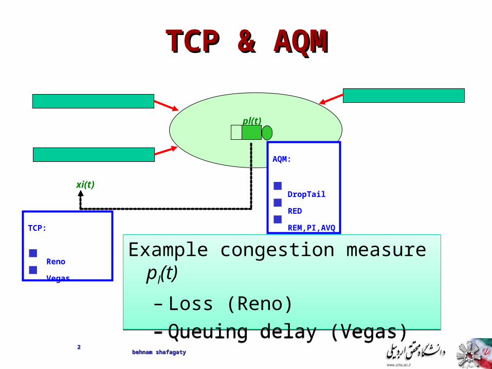
TCP & AQMTCP & AQM
xi(t)
pl(t)
TCP:
Reno
Vegas
AQM:
DropTail
RED
REM,PI,AVQ
Example congestion measure pl(t)
– Loss (Reno)– Queuing delay (Vegas)
Example congestion measure pl(t)
– Loss (Reno)– Queuing delay (Vegas)
22behnam shafagaty behnam shafagaty

Active queue managementActive queue management
• Main idea :: provide congestion information by some indications.
• Issues– How to measure congestion?– How to feed back congestion info?
33behnam shafagaty behnam shafagaty
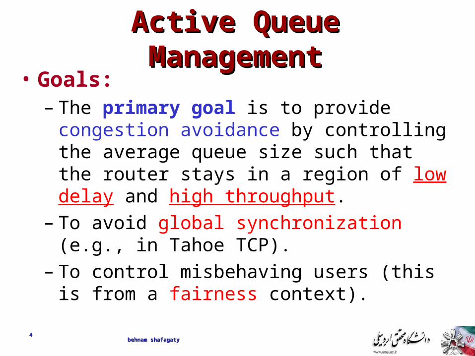
Active Queue Active Queue ManagementManagement
• Goals:– The primary goal is to provide
congestion avoidance by controlling the average queue size such that the router stays in a region of low delay and high throughput.
– To avoid global synchronization (e.g., in Tahoe TCP).
– To control misbehaving users (this is from a fairness context).
44behnam shafagaty behnam shafagaty
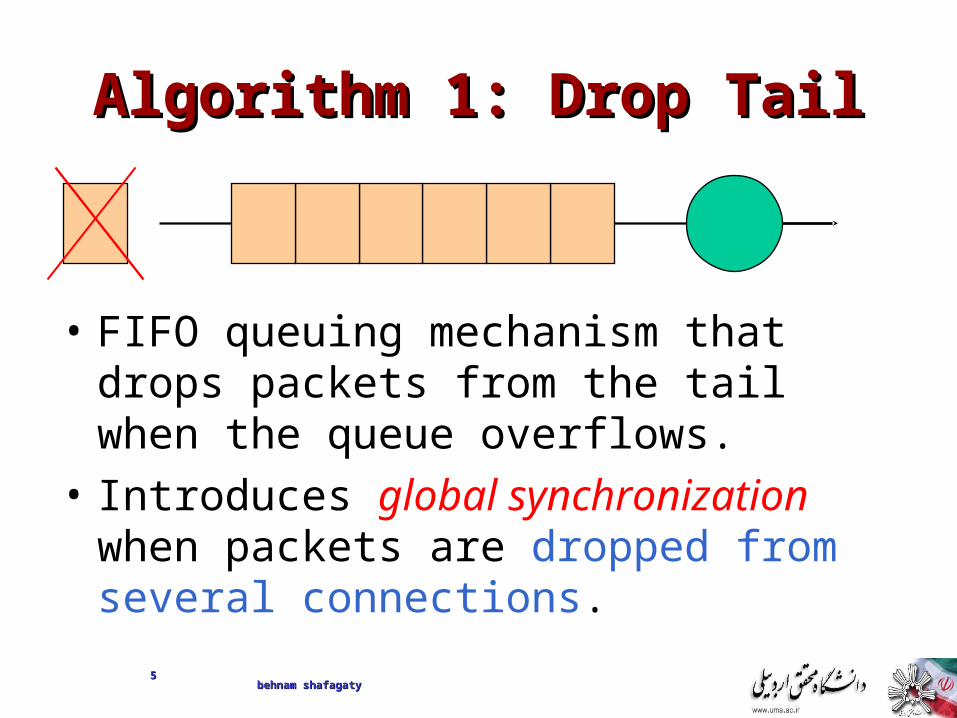
Algorithm 1: Drop TailAlgorithm 1: Drop Tail
55
• FIFO queuing mechanism that drops packets from the tail when the queue overflows.
• Introduces global synchronization when packets are dropped from several connections.
behnam shafagaty behnam shafagaty
66
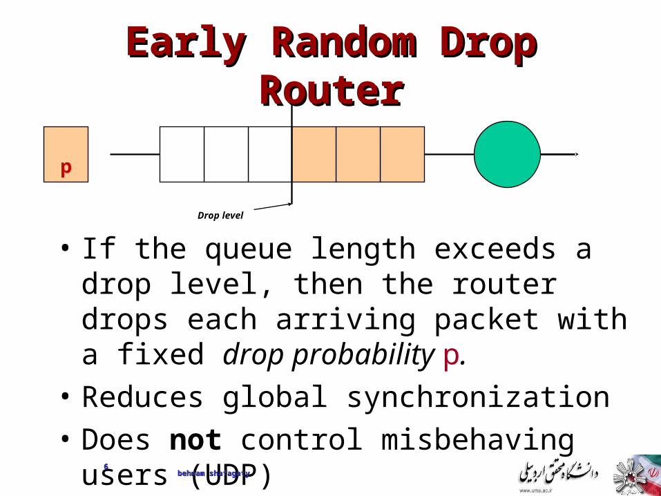
Early Random Drop Early Random Drop RouterRouter
• If the queue length exceeds a drop level, then the router drops each arriving packet with a fixed drop probability p.
• Reduces global synchronization
• Does not control misbehaving users (UDP)
p
Drop level
behnam shafagaty behnam shafagaty
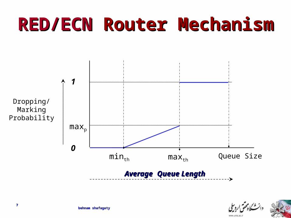
RED/ECNRED/ECN Router Router MechanismMechanism
77
1
0
AverageAverage Queue LengthQueue Length
minth maxth
Dropping/Marking
Probability
Queue Size
maxp
behnam shafagaty behnam shafagaty
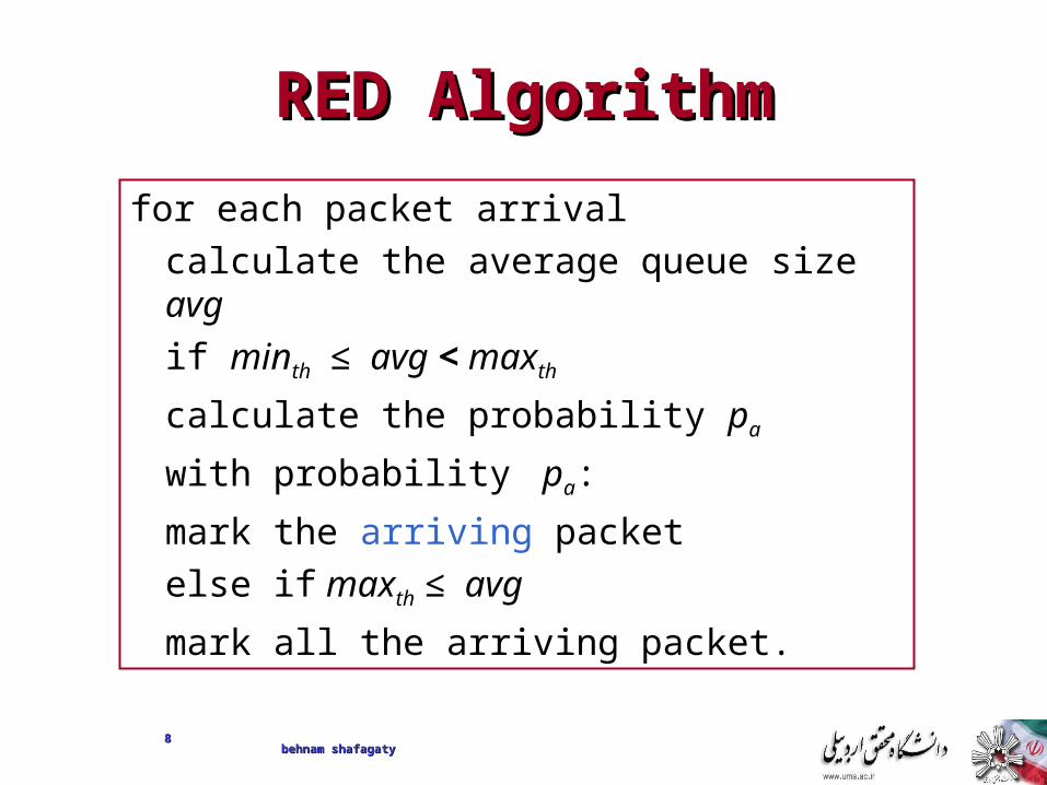
RED AlgorithmRED Algorithm
for each packet arrivalcalculate the average queue size avgif minth ≤ avg < maxth
calculate the probability pa
with probability pa:
mark the arriving packetelse if maxth ≤ avg
mark all the arriving packet.
behnam shafagaty behnam shafagaty 88
behnam shafagaty behnam shafagaty 99
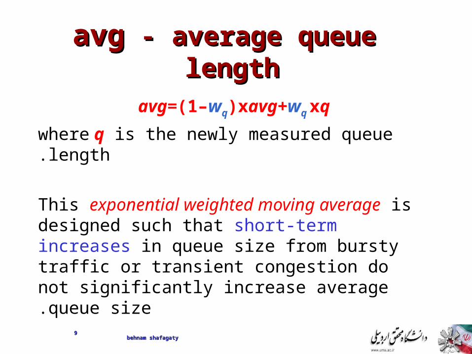
avgavg - average queue - average queue lengthlength
avg=(1–wq)xavg+wq xq
where q is the newly measured queue length.
This exponential weighted moving average is designed such that short-term increases in queue size from bursty traffic or transient congestion do not significantly increase average queue size.

behnam shafagaty behnam shafagaty 1010
REDRED drop probability drop probability ( ( ppa a ))
pb = maxp x (avg - minth)/(maxth – minth)
thenpa = pb/ (1 - count x pb)
Where, count is number of consecutive packets queued since last discard while in the critical region.
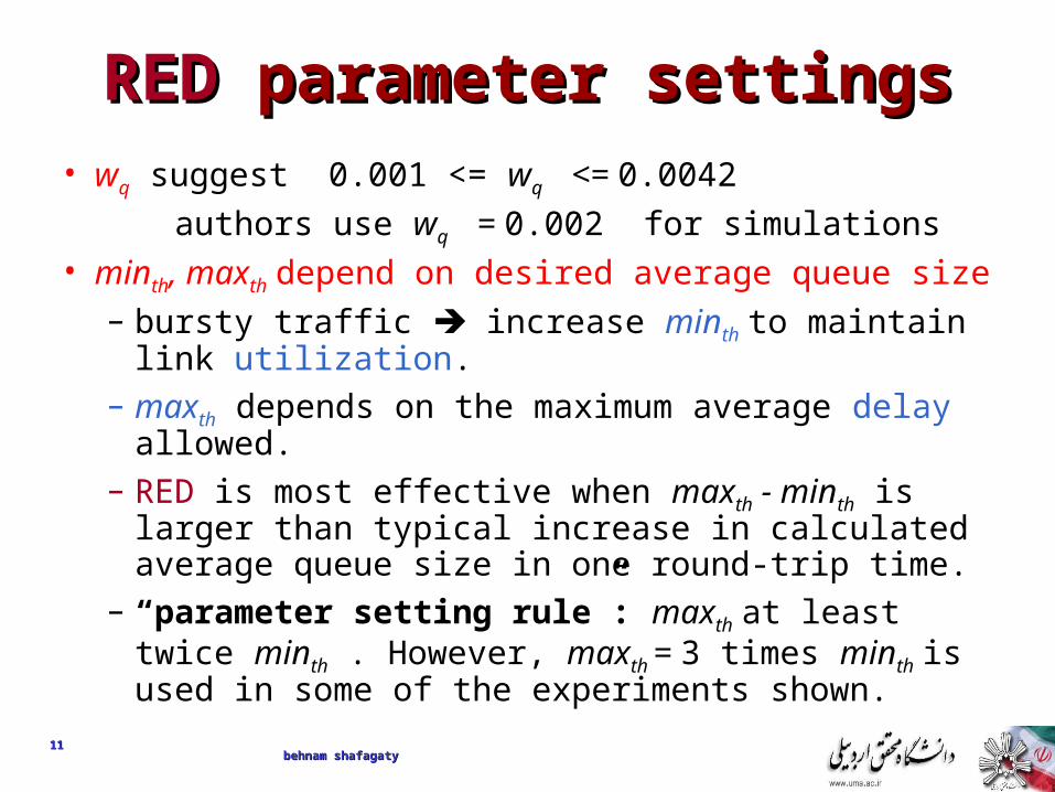
REDRED parameter settings parameter settings• wq suggest 0.001 <= wq <= 0.0042
authors use wq = 0.002 for simulations• minth, maxth depend on desired average queue size
– bursty traffic increase minth to maintain link utilization.
– maxth depends on the maximum average delay allowed.
– RED is most effective when maxth - minth is larger than typical increase in calculated average queue size in one round-trip time.
– “parameter setting rule”: maxth at least twice minth . However, maxth = 3 times minth is used in some of the experiments shown.
1111behnam shafagaty behnam shafagaty

Packet-marking probabilityPacket-marking probability
• The goal is to uniformly spread out the marked packets. This reduces global synchronization.
Method 1: geometric random variableWhen each packet is marked with probability pb,,
the packet inter-marking time, X, is a geometric random variable with E[X] = 1/pb.
• This distribution will both cluster packet drops and have some long intervals between drops!!
1212behnam shafagaty behnam shafagaty
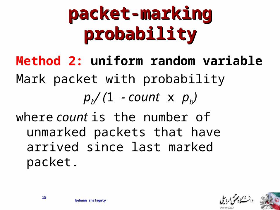
packet-marking probabilitypacket-marking probability
Method 2: uniform random variableMark packet with probability
pb/ (1 - count x pb)
where count is the number of unmarked packets that have arrived since last marked packet.
1313behnam shafagaty behnam shafagaty
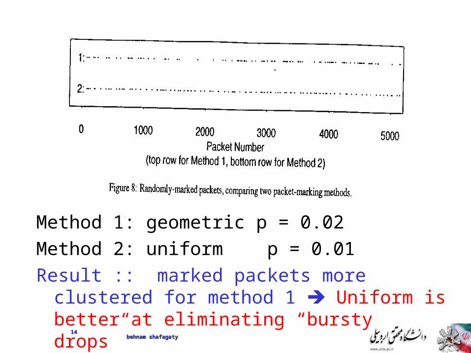
1414
Method 1: geometric p = 0.02Method 2: uniform p = 0.01Result :: marked packets more clustered for
method 1 Uniform is better at eliminating “bursty drops”
behnam shafagaty behnam shafagaty

Setting Setting maxmaxpp
• “RED performs best when packet-marking probability changes fairly slowly as the average queue size changes.”– This is a stability argument in that the claim is
that RED with small maxp will reduce oscillations in avg and actual marking probability.
• They recommend that maxp never be greater than 0.1
{This is not a robust recommendation.}
behnam shafagaty behnam shafagaty 1515
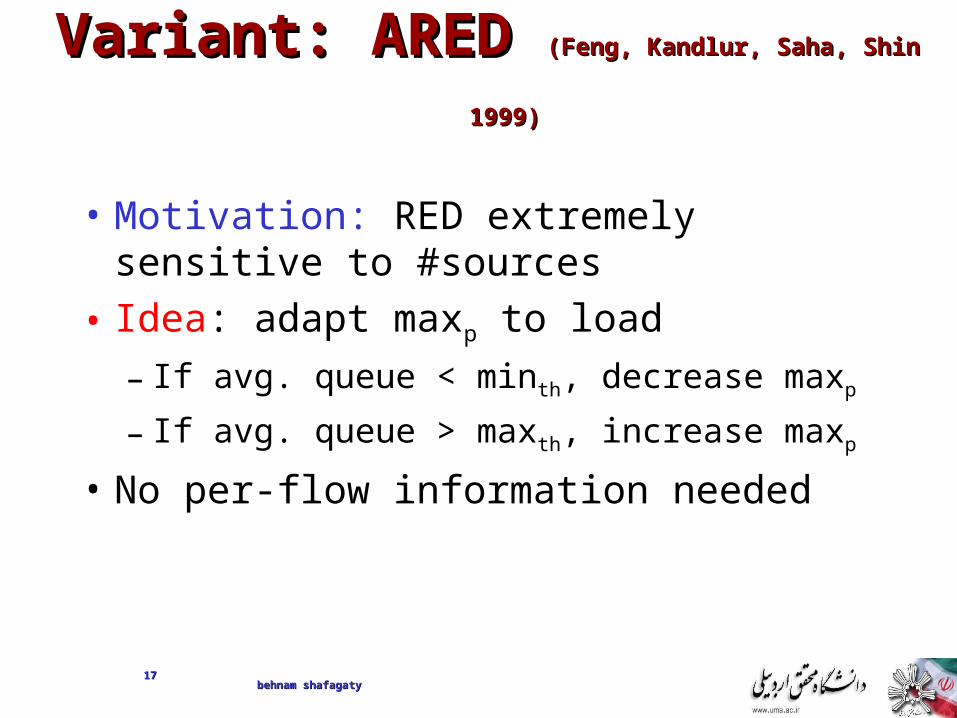
Variant: ARED Variant: ARED (Feng, Kandlur, Saha, Shin (Feng, Kandlur, Saha, Shin
1999)1999)
• Motivation: RED extremely sensitive to #sources
• Idea: adapt maxp to load
– If avg. queue < minth, decrease maxp
– If avg. queue > maxth, increase maxp
• No per-flow information needed
1717behnam shafagaty behnam shafagaty

Variant: FRED Variant: FRED (Ling & Morris 1997)(Ling & Morris 1997)
• Motivation: marking packets in proportion to flow rate is unfair (e.g., adaptive vs unadaptive flows)
• Idea:
– A flow can buffer up to minq packets without being marked
– A flow that frequently buffers more than maxq packets gets penalized
– All flows with backlogs in between are marked according to RED
– No flow can buffer more than avgcq packets persistently
• Need per-active-flow accounting1818
behnam shafagaty behnam shafagaty

Variant: SRED Variant: SRED (Ott, Lakshman & Wong (Ott, Lakshman & Wong
1999)1999) • Motivation: wild oscillation of queue in
RED when load changes• Idea:
– Estimate number N of active flows• An arrival packet is compared with a
randomly chosen active flows• N ~ prob(Hit)-1
– cwnd~p-1/2 and Np-1/2 = Q0 implies p = (N/Q0)2
• No per-flow information needed1919
behnam shafagaty behnam shafagaty

Variant: BLUE Variant: BLUE (Feng, Kandlur, Saha, Shin (Feng, Kandlur, Saha, Shin
1999)1999) Idea: perform queue management based directly on packet loss and link utilization rather than on the instantaneous or average queue lengths.
2020behnam shafagaty behnam shafagaty

REM REM (Athuraliya & Low 2000)(Athuraliya & Low 2000)
• Congestion measure: pricepl(t+1) = [pl(t) + g(al bl(t)+ xl
(t) - cl )]+
• Embedding: exponential probability function
• Feedback: dropping or ECN marking
0 2 4 6 8 10 12 14 16 18 200
0.1
0.2
0.3
0.4
0.5
0.6
0.7
0.8
0.9
1
Link congestion measure
Lin
k m
arkin
g probability
2121behnam shafagaty behnam shafagaty
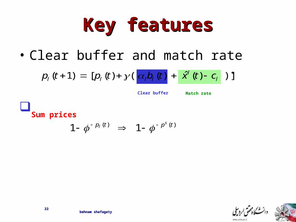
Match rate
Key featuresKey features
• Clear buffer and match rate
Clear buffer
)] )(ˆ )( ()([ )1( ll
llll ctxtbtptp
)()( 1 1 tptp sl
Sum prices
2222behnam shafagaty behnam shafagaty

TCP/AQM ModelsTCP/AQM Models
behnam shafagaty behnam shafagaty

TCP & AQMTCP & AQM
xi(t)
pl(t)
Example congestion measure pl(t)
– Loss (Reno)– Queueing delay (Vegas)
2626behnam shafagaty behnam shafagaty

Macroscopic View of TCP Macroscopic View of TCP ControlControl
•TCP/AQM: A feedback control system
TCP Sender 1TCP Sender 1C
xi(t)
TCP:
Reno
Vegas
FAST
AQM:
DropTail / RED
Delay
ECN
TCP Sender 2TCP Sender 2
q(t)
TCP Receiver 1TCP Receiver 1
TCP Receiver 2TCP Receiver 2
Bii tq,txFtx
ctxtqGtq Fi
i ,
τF
τB
2727behnam shafagaty behnam shafagaty
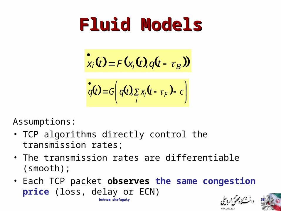
Fluid ModelsFluid Models
Assumptions:• TCP algorithms directly control the transmission
rates;• The transmission rates are differentiable (smooth);• Each TCP packet observes the same congestion
price (loss, delay or ECN)
Bii tq,txFtx
ctx,tqGtq Fi
i
2828behnam shafagaty behnam shafagaty
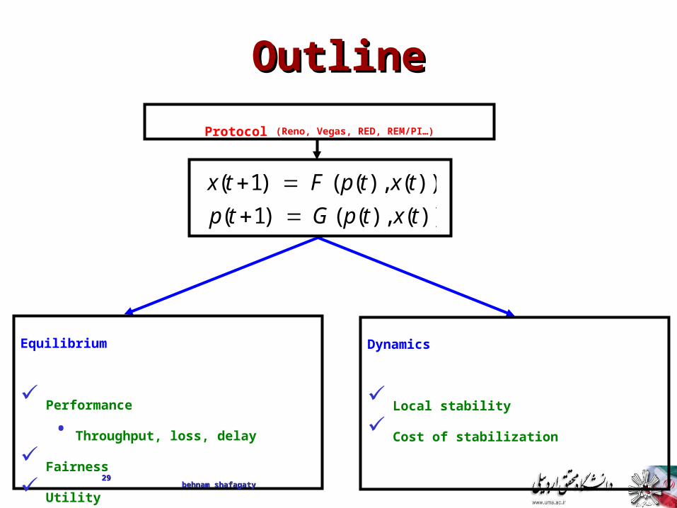
OutlineOutline
Protocol (Reno, Vegas, RED, REM/PI…)
Equilibrium
Performance
• Throughput, loss, delay
Fairness
Utility
Dynamics
Local stability
Cost of stabilization
))( ),(( )1(
))( ),(( )1(
txtpGtp
txtpFtx
2929behnam shafagaty behnam shafagaty


