Advanced Higher Physics Electromagnetism...

Advanced Higher

Physics

Electromagnetism

Notes

Name………………………………………………….

1 | P a g e Version 1.0


Key Area Notes, Examples and Questions

Page 3 Fields

Page 24 Circuits

Page 38 Electromagnetic Radiation

Other Notes

Page 41 Current, Mathematics and Right Hand Rules Page 43 Quantities, Units and Multiplication Factors Page 44 Relationships Sheets Page 49 Data Sheet


Key Area: Fields

Success Criteria 1.1 I can define electric field strength.

1.2 I can draw electric field patterns around single charges, a system of two charges and

a uniform electric field.

1.3 I can solve problems involving electric fields and the forces produced on charged

particles.

1.4 I can define electric potential.

1.5 I can state that the energy required to move a charge between two points in an

electric field is independent of the path taken.

1.6 I can solve problems involving electric potential.

1.7 I can solve problems on the motion and energy of charged particles in uniform

electric fields.

1.8 I know the definition of the Electron Volt (eV) and can convert between electron

volts and joules.

1.9 I explain the magnetic effect called ferromagnetism which occurs in certain metals.

1.10 I can draw magnetic field line patterns.

1.11 I can solve problems involving the magnetic induction formed around a current

carrying wire.

1.12 I can solve problems involving charged particles in magnetic fields in terms of their;

mass, velocity, charge, radius of their path and the magnetic induction of the

magnetic field.

1.13 I can solve problems involving the forces acting on a current carrying wire in a

magnetic field.

1.14 I can state comparisons between nuclear, electromagnetic and gravitational forces in

terms of relative magnitude and range.


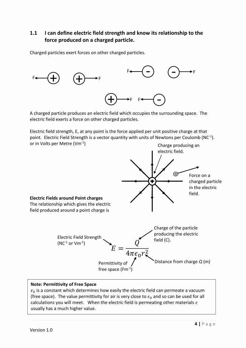
1.1 I can define electric field strength and know its relationship to the force produced on a charged particle.

Charged particles exert forces on other charged particles. A charged particle produces an electric field which occupies the surrounding space. The electric field exerts a force on other charged particles. Electric field strength, E, at any point is the force applied per unit positive charge at that point. Electric Field Strength is a vector quantity with units of Newtons per Coulomb (NC-1). or in Volts per Metre (Vm-1) Electric Fields around Point charges The relationship which gives the electric field produced around a point charge is

𝐸 =𝑄

4𝜋𝜖0𝑟2

Electric Field Strength (NC-1 or Vm-1)

Charge of the particle producing the electric field (C).

Distance from charge Q (m) Permittivity of free space (Fm-1)

Note: Permittivity of Free Space 𝜖0 is a constant which determines how easily the electric field can permeate a vacuum (free space). The value permittivity for air is very close to 𝜖0 and so can be used for all calculations you will meet. When the electric field is permeating other materials 𝜖 usually has a much higher value.

+ + F F

+ - F F

-

-

F F

Charge producing an electric field.

Force on a charged particle in the electric field.


Forces Produced by Electric Fields The relationship between the force produced on a charged particle in an electric field, charge and electric field strength is given by the relationship Forces - Point Charges

Both the relationships 𝐹 = 𝑄𝐸 and E =Q

4𝜋𝜖0𝑟2 can be combined to give Coulomb′s Law

Note that 𝑄 in each of these two relationships refer to different charges.

Forces - Uniform Electric fields

When performing calculations with uniform fields between charged plates 𝑉 = 𝐸𝑑 is usually used as the voltage across the plates is usually known.

𝐹 = 𝑄𝐸

Electric Field Strength (NC-1 or Vm-1)

Charge on the particle in the electric field (C)

Force (N)

𝐹 =𝑄1𝑄2

4𝜋𝜖0𝑟2

Electric Force (N)

Charge of the particle producing the electric field (C).

Distance of 𝑄1 from 𝑄2 (m)

Permittivity of free space (Fm-1)

Charge on the particle in the electric field (C)

Note Like Newton’s Law of Gravitation, Coulomb’s Law is an inverse square law.

-

+ F

From the Higher Physics course

𝐸𝑤 = 𝐹𝑑 and 𝐸𝑊 = 𝑄𝑉

Combining these gives

𝐹 =𝑄𝑉

𝑑

Equating this to the definition of an electric

field, 𝐹 = 𝑄𝐸 gives

𝑄𝑉

𝑑= 𝑄𝐸

Which simplifies to

𝑉 = 𝐸𝑑


1.2 I can draw electric field patterns around single charges, a system of two charges and a uniform electric field.

Also see Higher Physics Particle and Waves Notes section 2.2.

Single positive charge Single negative charge

+ - Two opposite charges

Two positive charges

+ +


Parallel plates produce a uniform field between the plates. The curvature of the field lines at the edges of the plates is small and frequently not shown in diagrams.

Parallel Charged Plates

- -

Two negative charges


1.3 I can solve problems involving electric fields and the forces produced on charged particles.

Example 1 Find the magnitude of electric field strength at the Bohr radius (5.29 × 10−11m) of a

hydrogen atom.

Solution 1

𝑟 = 5.29 × 10−11m

𝜖0 = 8.85 × 10−12Fm−1

𝑄 = 1.6 × 10−19C

Electromagnetism problem book pages 6 and 7, questions 1 to 7. Example 2 - Electric Dipole The diagram below shows two charged particles in an arrangement called an electric dipole. Find the electric field at point P. Solution 2 – Electric Dipole

𝑟+ = 𝑟− = √(9.0 × 10−10)2 + (1.0 × 10−9)2 = 1.345 × 10−9m Electric field due to the positive charge

𝐸+ =𝑄+

4𝜋𝜖0𝑟+2 =

5.0 × 10−10

4 × 𝜋 × 8.85 × 10−12 × (1.345 × 10−9)2= 2.485 × 1018NC−1

𝐸 =𝑄

4𝜋𝜖0𝑟2

𝐸 =1.6 × 10−19

4𝜋 × 8.85 × 10−12 × 5.29 × 10−11

𝐸 = 27NC−1

+

-

P

𝑟+

𝑟−

5.0 × 10−10C

−5.0 × 10−10C 1.0 × 10−9m

9.0 × 10−10m

9.0 × 10−10m


Electric field due to the negative charge

𝐸+ =𝑄+

4𝜋𝜖0𝑟−2

=−5.0 × 10−10

4 × 𝜋 × 8.85 × 10−12 × (1.345 × 10−9)2= −2.485 × 1018NC−1

To find the resultant electric field first find the angle 𝜃.

tan 𝜃 =9.0 × 10−10

1.0 × 10−9

𝜃 = tan−1 (9.0 × 10−10

1.0 × 10−9) = 41.99°

Using the cosine rule

𝐸𝑅 = √|𝐸−|2 + |𝐸+|2 − 2|𝐸−||𝐸+| cos 2𝜃

As |𝐸−|2 = |𝐸+|2 = |𝐸|2 and |𝐸−||𝐸+| = |𝐸|2

𝐸𝑅 = √2|𝐸|2 − 2|𝐸|2 cos 2𝜃

𝐸𝑅 = |𝐸|√2(1 − cos 2𝜃)

𝐸𝑅 = 2.485 × 1018 × √2(1 − cos(2 × 41.99))

𝐸𝑅 = 3.3 × 1018NC−1 vertically downward

Electromagnetism problem book page 9, question 13.

P

𝑟+

1.0 × 10−9m

9.0 × 10−10m 𝐸−

𝐸+

𝐸𝑅 𝜃 2𝜃 +

-

P

𝑟+

𝑟−

1.0 × 10−9m

9.0 × 10−10m

𝐸−

𝐸+

The resultant electric field 𝐸𝑅 is given by the vector addition of 𝐸− and 𝐸−.

9.0 × 10−10m

𝐸𝑅

A a

b

B c

C

𝑎2 = 𝑏2 + 𝑐2 − 2𝑏𝑐 cos 𝐴

Cosine Rule

𝑎 = √𝑏2 + 𝑐2 − 2𝑏𝑐 cos 𝐴


Example 3 – Coulomb’s Law

Helium He24 consists of two protons and two neutrons. Calculate the ratio,

Electrostaic Force

Gravitational Force,

for the two protons when they are 10−15m apart. Solution 3 – Coulomb’s Law Electric Force

𝐹𝐸 =𝑄1𝑄2

4𝜋𝜖0𝑟2=

1.6 × 10−19 × 1.6 × 10−19

4𝜋 × 8.85 × 10−12 × (10−15)2= 230N

Gravitational Force

𝐹𝐺 =𝐺𝑚1𝑚2

𝑟2=

6.67 × 10−11 × 1.673 × 10−27 × 1.673 × 10−27

(10−15)2= 1.87 × 10−34N

𝐹𝐸

𝐹𝐺=

230

1.87 × 10−34= 1.2 × 1036

Note how the electric force is much larger than the gravitational force. Example 4 – Coulomb’s Law Three charged objects are fixed in position. Each has a charge of+120𝜇C. Calculate the magnitude of the force on charge 2.

Solution 4 Coulomb’s Law Force on charge 2 due to charge 3

𝐹23 =𝑄2𝑄3

4𝜋𝜖0𝑟2=

120 × 10−6 × 120 × 10−6

4𝜋 × 8.85 × 10−12 × 2.02= 32.37N

Force on charge 2 due to charge 1

𝐹21 =𝑄2𝑄3

4𝜋𝜖0𝑟2=

120 × 10−6 × 120 × 10−6

4𝜋 × 8.85 × 10−12 × 1.02= 129.5N

Force 𝐹23 and 𝐹21 are both vectors

𝐹𝑅 = √129.52 + 32.372 = 133N

Electromagnetism problem book pages 4 to 6, questions 1 to 11; page 8 question 10

2 3

1

2.0m

1.0m

2

129.5N

32.37N

129.5N

32.37N

𝐹𝑅


Example 5 – Uniform Electric Fields Two charged plates 1.0cm apart have a voltage of 4000V placed across them. a. Find the electric field strength between

the two plates. b. If an electron is placed between the

plates, calculate the electric force on the electron.

Solution Example 5 – Uniform Electric Fields. a. 𝑑 = 1.0cm = 0.01m

𝑉 = 𝐸𝑑 ⇒ 𝐸 =𝑉

𝑑

𝐸 =4000

0.01= 4.0 × 105Vm−1

b. 𝐹 = 𝑄𝐸

𝐹 = 1.6 × 10−19 × 4.0 × 105

𝐹 = 6.4 × 10−14N

Electromagnetism problem book pages 7 to 9, questions 8, 9, 11 to 13.

-

+ F


1.4 I can define electric potential. Electric potential at a point is the work done in moving a unit positive charge 𝑄𝑡 from infinity to that point. Note the similarity between this definition and the definition of gravitational potential.

1.5 I can state that the energy required to move a charge between two points in an electric field is independent of the path taken.

From the electric potential relationship, the electric potential energy of a unit charge depends on the distance from the charge producing the field. The distances between the initial and final positions determine the energy required to move the charge. Whether the charge follows path 1 or path 2 the energy change will be the same.

𝑉 =𝑄

4𝜋𝜖0𝑟

Electric potential (V) Distance (m)


Charge (C) Note Electric potential is a scalar quantity.

𝑟

∞

𝑄𝑡 𝑄𝑡

Charge producing the electric field

Final distance

distance, r

Initial distance


1.6 I can solve problems involving electric potential. Example 1 Calculate the electric potential at point P midway between the two charges. Solution 1

𝑟 =1.0

2= 0.50m

𝑉1 =𝑄

4𝜋𝜖0𝑟=

100 × 10−12

4𝜋 × 8.85 × 10−12 × 0.50= 1.80V

𝑉2 =𝑄

4𝜋𝜖0𝑟=

−400 × 10−12

4𝜋 × 8.85 × 10−12 × 0.50= −7.19V

Potential at P

𝑉𝑃 = 1.80 − 7.19 = −5.4V

Example 2 Three small charges are each 4.0cm from the point P. Calculate the electric potential at point P. Solution 2 𝑟 = 4.0cm = 0.04m

𝑉1 =𝑄

4𝜋𝜖0𝑟=

3.0 × 10−9

4𝜋 × 8.85 × 10−12 × 0.04= 674.4V

𝑉2 =𝑄

4𝜋𝜖0𝑟=

−5.0 × 10−9

4𝜋 × 8.85 × 10−12 × 0.04= −1124V

𝑉3 =𝑄

4𝜋𝜖0𝑟=

2.0 × 10−9

4𝜋 × 8.85 × 10−12 × 0.04= 449.6V

Potential at P

𝑉𝑃 = 674.4 − 1124 + 449.6 = 0V

Electromagnetism problem book pages 9 to 11, questions 1 to 14.

2

1

P 3 2.0nC

-5.0nC

3.0nC

2 1 P -400pC 100pC

1.0m


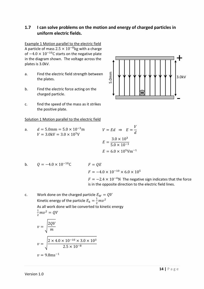
1.7 I can solve problems on the motion and energy of charged particles in uniform electric fields.

Example 1 Motion parallel to the electric field A particle of mass 2.5 × 10−8kg with a charge of −4.0 × 10−10C starts on the negative plate in the diagram shown. The voltage across the plates is 3.0kV. a. Find the electric field strength between

the plates. b. Find the electric force acting on the

charged particle. c. find the speed of the mass as it strikes

the positive plate. Solution 1 Motion parallel to the electric field a. 𝑑 = 5.0mm = 5.0 × 10−3m 𝑉 = 3.0kV = 3.0 × 103V

b. 𝑄 = −4.0 × 10−10C c. Work done on the charged particle 𝐸𝑊 = 𝑄𝑉

Kinetic energy of the particle 𝐸𝑘 =1

2𝑚𝑣2

As all work done will be converted to kinetic energy

1

2𝑚𝑣2 = 𝑄𝑉

𝑣 = √2𝑄𝑉

𝑚

𝑣 = √2 × 4.0 × 10−10 × 3.0 × 103

2.5 × 10−8

𝑣 = 9.8ms−1

-

+

3.0kV

5.0

mm

𝑉 = 𝐸𝑑 ⇒ 𝐸 =𝑉

𝑑

𝐸 =3.0 × 103

5.0 × 10−3

𝐸 = 6.0 × 105Vm−1

𝐹 = 𝑄𝐸

𝐹 = −4.0 × 10−10 × 6.0 × 105

𝐹 = −2.4 × 10−4N The negative sign indicates that the force is in the opposite direction to the electric field lines.


Example 2 Motion perpendicular to the electric field An electron in an oscilloscope is fired at a speed of 1.0 × 106ms−1 through charged deflection plates of length 10mm. If the strength of the electric field between the plates is 1.0 × 104NC−1, calculate the deflection, s, of the electron when leaving the plates.

Solution 2 Motion perpendicular to the electric field x-direction Calculate the time taken for the electron to pass the length of the plates. The component of the electron’s velocity in the x-direction is constant as the electric field will accelerate the electron vertically. 𝑑 = 10mm = 10 × 10−3m y-direction

Find the y-direction acceleration then use 𝑠 = 𝑢𝑡 +1

2𝑎𝑡2 to find the displacement.

𝑎 =𝐹

𝑚 and 𝐹 = 𝑄𝐸

𝑎 =𝑄𝐸

𝑚

𝑎 =1.6 × 10−19 × 1.0 × 104

9.11 × 10−31

𝑎 = 1.76 × 1015ms−1

Substituting 𝑎 into 𝑠 = 𝑢𝑡 +1

2𝑎𝑡2

𝑠 = 0 × 1.0 × 10−8 +1

2× 1.76 × 1015 × (1.0 × 10−8)2

𝑠 = 0.088m Electromagnetism problem book pages 13 to 17, questions 1 to 12.

-

+

x

y

s

d=10mm

𝑠 = 𝑣𝑡 ⇒ 𝑡 =𝑠

𝑣

𝑡 =10 × 10−3

1.0 × 106

𝑡 = 1.0 × 10−8s


1.8 I know the definition of the Electron Volt (eV) and can convert between electron volts and joules.

The electron volt (eV) is a unit of energy not voltage. It is defined as the work done on an electron as it is moved between two points with potential difference of 1 volt.

𝐸𝑤 = 𝑄𝑉 𝐸𝑤 = 1.6 × 10−19 × 1 = 1.6 × 10−19J

The electron volt is frequently used when dealing with the energy of subatomic particles and atomic processes. It is also used with 𝐸 = 𝑚𝑐2 to express the mass of subatomic particles in terms of energy. To convert joules to electron volts divide by 1.6 × 10−19. To convert from electron volts to joules multiply by 1.6 × 10−19. Electromagnetism problem book page 18, questions 16 to 19.

1.9 I explain the magnetic effect called ferromagnetism which occurs in

certain metals. The motion of electrons in around the nucleus produce a magnetic dipole similar to a bar magnet. In most materials, the magnetic fields produced by the electrons cancel to produce no effect. In some materials, the magnetic fields of each atom combine to produce an overall ferromagnetic effect. The magnetic fields produced by groups of atoms form regions called domains. In each domain, the magnetic fields of the atoms all line up in the same direction. This effectively makes each domain a dipole magnet. Material in which magnetic domains form are called ferromagnetic. There are few ferromagnetic materials. Examples are iron, nickel and cobalt.

S

N


Diagram 1 shows a ferromagnetic material where the magnetic domains are aligned randomly. The magnetic fields cancel leaving the material unmagnetized. Diagram 2 shows a ferromagnetic material after being affected by an external magnetic field. The atoms within the magnetic domains are rotated to align with the externally applied magnetic field. This alignment remains after the external magnetic field is removed leaving the material magnetised. It is now a permanent magnet. in this case some domains remain randomly orientated and some are aligned. This means that the material is only partially magnetised. Diagram 3 shows a material where all the magnetic domains have been aligned using a strong external magnetic field. This leaves a strong saturated magnet. The magnetisation of the saturated magnet cannot be further increased. Demagnetisation Anything that disrupts the alignment of the domains will demagnetise a permanent magnet. This can be done by

placing the magnet in an external alternating magnetic field. This is a common way to demagnetise materials.

repeatedly striking the magnet.

heating the magnet above its curie temperature. Above this temperature the atoms in the ferromagnetic material have sufficient kinetic energy to rotate to random directions.

Electromagnetism problem book page 19, questions 1 to 4.

Randomly orientated domains. The material is not magnetised.

All domains aligned. Material is magnetised

and saturated.

No

rth

Sou

th

Most domains aligned. Material is partially

magnetised but unsaturated. N

ort

h

Sou

th

Diagram 1 Diagram 2 Diagram 3


1.10 I can draw magnetic field line patterns. Magnetic field lines point from north to south. The spacing between the field line indicates the strength on the magnetic field. The closer the lines the stronger the field.

N S

S S N N

N N S S

S S N N


Coil of Wire

Solenoid A solenoid (inductor) consists of a coil of wire. Passing a current through the coil produces a magnetic field.

Earth’s Magnetic Field The Earth’s liquid iron rich core produces currents which create a magnetic field. This field is similar in shape to a dipole magnet in the core of the Earth.

Magnetic field around a moving positive charge.

Magnetic field around a moving negative charge.


1.11 I can solve problems involving the magnetic induction formed around a current carrying wire.

Current in a wire produces a magnetic field which forms closed loops around the wire. The direction of the magnetic field is given by the right-hand rule. The thumb follows the direction of the conventional current. The curl of the fingers gives the direction of the magnetic field. The strength of the magnetic field is called the magnetic induction and is given by Example When a voltage of 6.0V is placed across the ends of a straight wire a magnetic induction of 1.5 × 10−5T is formed at 10mm from a wire. Find the resistance of the wire. Solution 𝜇0 = 4𝜋 × 10−7Hm−1 𝑟 = 10mm = 10 × 10−3m 𝐵 = 1.5 × 10−5T Electromagnetism problem book page 21, questions 1 to 4.

Conventional Current flows from positive to negative.

Electrons flow from negative to positive.

𝐵 =𝜇0𝐼

2𝜋𝑟

Magnetic Induction (T)

Current (A)

Distance from the wire (m)

Permeability of free space (Hm-1)

𝐵 =𝜇0𝐼

2𝜋𝑟 ⇒ 𝐼 =

2𝜋𝑟𝐵

𝜇0

𝐼 =2𝜋 × 10 × 10−3 × 1.5 × 10−5

4𝜋 × 10−7

𝐼 = 0.75A

𝑉 = 𝐼𝑅 ⇒ 𝑅 =𝑉

𝐼

𝑅 =6.0

0.75

𝑅 = 8.0Ω

Magnetic induction is measured in Tesla (T).


1.12 I can solve problems involving charged particles in magnetic fields in terms of their; mass, velocity, charge, radius of their path and the magnetic induction of the magnetic field.

This is covered in section 2.4 of the Quanta and Waves Notes.

1.13 I can solve problems involving the forces acting on a current carrying wire in a magnetic field.

When a current carrying wire is placed in magnetic field there will be a force on the wire. In section 2.4 in quanta and waves the force on moving charged particles in a magnetic field was found using the relationship 𝐹 = 𝑞𝑣𝐵. This can be extended to the charges moving in a wire giving the relationship below. The direction of the force on the wire can be found using the right-hand rule given in section 2.4 of quanta and waves. This must be done with the velocity direction given by the direction of the conventional current.

𝐹 = 𝐼𝑙𝐵 sin 𝜃

Force on the wire (N)

Length of the wire (m)

Magnetic Induction (T)

Current (A)

Angle between the wire and the magnetic induction (°)

𝐼 -conventional current

B


Example 1 A wire carrying a current of 6.0 A has 0.50 m of its length placed in a magnetic field of magnetic induction 0.20 T. Calculate the size of the force on the wire if it is placed:

a. at right angles to the direction of the field b. at 45° to the direction of the field c. along the direction of the field (i.e. lying parallel to the field lines). Solution 2 a. When the field is at a right angle to the wire 𝜃 = 90°. 𝐹 = 𝐼𝑙𝐵 sin 𝜃 𝐹 = 6.0 × 0.50 × 0.20 × sin 90° = 0.60N b. 𝐹 = 6.0 × 0.50 × 0.20 × sin 45° = 0.42N c. 𝜃 = 0°, sin 0° 0, so 𝐹 = 0𝑁 Example 2

Two wires each carrying 2.0A are placed 20mm apart. a. Calculate the force produced on wire 2. b. Do the wires attract or repel each other? Solution 2

a. Use 𝐵 =𝜇0𝐼

2𝜋𝑟 to find magnetic induction at wire 2.

Then use 𝐹 = 𝐼𝑙𝐵 sin 𝜃 to find the force on the wire. 𝐼 = 2.0A 𝑟 = 20mm = 20 × 10−3m 𝜃 = 90° b. Wires attract. Use the right hand rule from section 2.4 in the Quanta and Waves

Notes. Electromagnetism problem book pages 21 to 26, questions 1 to 13.

𝐵 =𝜇0𝐼

2𝜋𝑟

𝐵 =4𝜋 × 10−7 × 2.0

2𝜋 × 20 × 10−3

𝐵 = 2.0 × 10−5T

𝐹 = 𝐼𝑙𝐵 sin 𝜃

𝐹 = 2.0 × 1.2 × 2.0 × 10−5

× sin 90°

𝐹 = 4.8 × 10−5N

𝐼

𝐼


1.14 I can state comparisons between nuclear, electromagnetic and gravitational forces in terms of relative magnitude and range.

The table below compares the relative strength of the nuclear, electromagnetic and gravitational forces taking the nuclear force to have a value of 1.

Force Relative

Magnitude Range (metres)

Strong 1 10−15

Electromagnetic 10−3 Infinite

Gravity 10−41 Infinite


Key Area: Circuits

Success Criteria

2.1 I can describe the variation of current and potential difference with time in a CR

circuit during charging and discharging.

2.2 I can define the time constant for a CR circuit and use this to and solve problems.

2.3 I can define capacitive reactance.

2.4 I can solve problems involving capacitive reactance, voltage, current frequency and

capacitance.

2.5 I understand how an inductor is constructed.

2.6 I understand electromagnetic induction and the factors which affect the induction of

a current in an inductor.

2.7 I can state what is meant by the self-inductance of a coil.

2.8 I know the effect of placing an iron core inside an inductor.

2.9 I understand Lenz’s law and the effect back E.M.F has on the current in a circuit.

2.10 I can solve problems involving back E.M.F and the energy stored in a capacitor.

2.11 I can define inductive reactance.

2.12 I can solve problems involving inductive reactance, voltage, current frequency and

inductance.


2.1 I can describe the variation of current and potential difference with time in a CR circuit during charging and discharging.

See section 4.8 and 4.9 in the Higher Physics Electricity notes The circuit shown contains a capacitor and resistor in series. This is a CR circuit. When switch S is moved to position A the capacitor charges. When moved to position B the capacitor discharges. The graphs of current potential difference and against time across the capacitor against time are shown below. Charging Discharging Revision of higher physics capacitors Electromagnetism problem book pages 27 to 30, questions 1 to 7.

Switch in position B. The capacitor is discharging. The voltage falls towards zero from an initial value of ℰ. The current has an initial value of

−ℰ

𝑅 which falls towards zero. Time 0

Capacitor P.d.

ℰ

Time 0

Current

ℰ

𝑅

Current is negative as it is flowing in the opposite direction to the charging current.

Time 0

Capacitor P.d.

ℰ

Time 0

Current

ℰ

𝑅

Switch in position A. The capacitor is charging. The voltage rises from zero until it reaches the e.m.f. of the battery, ℰ.

The current has an initial value of ℰ

𝑅

which falls towards zero.

ℰ

V

R

A

A

B Switch, S


2.2 I can define the time constant for a CR circuit and use this to and solve problems.

In a circuit containing a capacitor and resistor, the relationships which define the charging current and potential difference across a capacitor are

𝐼 =𝑉𝐶

𝑅𝑒−

𝑡𝑅𝐶 and 𝑉𝐶 = 𝑉𝑆 [1 − 𝑒−

𝑡𝑅𝐶]

Where 𝑉𝑠 - EMF of the supply

𝑉𝐶 - potential difference across the capacitor

𝑅 - resistance in the circuit

𝐼 - Charging current

𝐶 – Capacitance in the circuit

The term 𝑅𝐶 in these relationships is called the time constant.

A large value of time constant gives a long charging and discharging time.

A small value of time constant give a short charging and discharging time.

The exponential relationship of the charging curves means that the time taken for the voltage to reach the EMF of the supply and the charging current to decrease to zero is not easily determined. The time constant is used to make the charging and discharging times of CR circuits easy to compare.

R

𝑉𝑠

You do not need to know or be able to use these relationships.

𝑡 = 𝑅𝐶 Time Constant (s)

Resistance (Ω)

Capacitance (F)

Note The 𝑡 in this relationship is a constant. It is a different quantity to the variable 𝑡 in the above relationships for 𝐼 and 𝑉𝐶.


When the capacitor is charging the time constant represents the time taken for

the voltage across the capacitor to increase to 63% of the supply EMF.

The current in the circuit to decrease by 63% to 37% of the initial charging current.

When the capacitor is discharging the time constant represents the time taken for

the voltage across the capacitor to decrease by 63% to 37% of the supply EMF.

The current in the circuit to decrease by 63% to 37% of the initial discharge current.

Time (s) 0

Voltage (V)

𝑉𝐶 = 𝑉𝑆 [1 − 𝑒−𝑡

𝑅𝐶]

𝑡

𝑅𝐶

Time (s) 0

Current (A)

𝐼 =𝑉𝐶

𝑅𝑒−

𝑡𝑅𝐶

𝑡

𝑅𝐶

63% of 𝑉𝑆

37% of 𝑉𝑆

𝑅

Capacitor Charging

Time (s) 0

Current (A)

𝑡

𝑅𝐶

37% of 𝑉𝑆

𝑅

Time (s) 0

Voltage (V)

𝑡

𝑅𝐶

37% of 𝑉𝑆

Capacitor Discharging

𝑉 = 𝑉𝑆 𝑒−𝑡

𝑅𝐶

𝐼 = −𝑉𝐶

𝑅𝑒−

𝑡𝑅𝐶


Example 1 You are given the following components.

10MΩ Resistor 20μF Capacitor 1MΩ Resistor 20pF Capacitor 10kΩ Resistor 20nF Capacitor

a. Which the combination of a single resistor and single capacitor in series give the longest charging time.

b. Calculate the time constant for the combination found in part a. Solution 1 a. For the longest time the time constant, 𝑅𝐶, must be have the largest value. 𝑅 and 𝐶

have the largest values so choose 10MΩ resistor and a 20μF capacitor. b. 𝑡 = 𝑅𝐶 𝑡 = 10 × 106 × 10 × 10−6 𝑡 = 100s Example Finding the time constant from a graph

The variation of potential difference across a capacitor in a of an RC circuit as it discharges is shown below. The time constant for this circuit can be found by

Reading the initial voltage 𝑉𝐶.

Calculating 37% of 𝑉𝐶 .

Tracing a line from 37% of 𝑉𝐶 to the graph line then down to the time axis.

Reading the time constant value from the time axis.


0 10 20 30 40 50 60 70 80 90 100 Time (s)

0

7.0

6.0

5.0

4.0

3.0

2.0

1.0

Pote

nti

al D

iffe

ren

ce (

V)

𝑉𝐶 = 6.2V

Read the time constant from the time axis. 𝑡 = 29s

37% of 𝑉𝐶 =37

100× 6.2 = 2.3V

Project a line from 2.3V to the graph line then to the time axis.


2.3 I can define capacitive reactance. Capacitive reactance is the opposition to a.c. current by the capacitance of a capacitor. In a circuit containing resistance only, the frequency of the supply has no effect on the current in the circuit Ohm’s Law applies to resistance only circuits

So R =𝑉𝐶

𝐼

In a circuit containing a resistor and capacitor (an RC circuit) the current depends on the frequency of the supply. The resistance in an RC circuit is fixed. The quantity capacitive reactance is defined to take into account the variation in current with frequency.

R

𝑉𝐶

~

Frequency

Current

R

𝑉𝐶

~

Frequency

Current

𝑋𝐶 =𝑉

𝐼

Capacitive Reactance (Ω)

Voltage across the capacitor (V)

Current (A)

𝑋𝐶 =1

2𝜋𝑓𝐶

Capacitive Reactance (Ω)

Supply frequency (Hz)

Capacitance (F)

Compare with inductive reactance in section 2.11.


2.4 I can solve problems involving capacitive reactance, voltage, current frequency and capacitance.

Example 1 The circuit shown runs from the UK mains at 230V, 50Hz. Calculate the capacitive reactance in the circuit. Solution 1 𝑓 = 50Hz 𝐶 = 30mF = 30 × 10−3F 𝑉 = 230V

𝑋𝐶 =1

2𝜋𝑓𝐶

𝑋𝐶 =1

2𝜋 × 50 × 30 × 10−3

𝑋𝐶 = 0.11Ω

Example A circuit containing capacitive components is designed in the US to operate at 100V derived from mains 60Hz supply. It is shipped to the UK where it is operated at 100V derived from the main 50Hz supply. It is found that the power output from the circuit is reduced. Explain why. Solution The frequency of the supply is decreased so the capacitive reactance in the circuit will be

increased as 𝑋𝐶 =1

2𝜋𝑓𝐶. As the capacitive reactance is increased the current in the circuit

will decrease as 𝑋𝐶 =𝑉

𝐼. The reduced current reduces the power output of the circuit.


R

230V

~

30mF


2.5 I understand how an inductor is constructed. An inductor consists of a coil of wire which can contain and metal core

The inductance of an inductor depends on

The number of turns per metre. The greater the number of turns per meter the larger the inductance.

Having an iron core. Inductors with an iron core have a higher inductance than an inductor without a core.

2.6 I understand electromagnetic induction and the factors which affect the induction of a current in an inductor.

Magnetic induction occurs when the movable charges in a conductor are subject to a changing magnetic field. This causes them to move producing an electrical current. The diagram below shows a magnet being moved in and out of a coil of wire. This will produce a voltage reading on the voltmeter. The factors which affect the voltage produced are:

The speed of the magnet. The faster the magnet the greater the rate of change of the magnetic field, the greater the induced voltage.

The strength of the magnetic field. The greater the magnetic field the greater the voltage induced.

Number of turns on the coil. The greater the number of turns the larger the voltage produced.

Direction of the magnet field. Reversing the magnet reverses the polarity of the voltage.

Direction of motion. Reversing the direction of motion of the magnet reverses the polarity of the voltage.

Symbol for an inductor with a core

Symbol for an inductor without a core

S N

Voltmeter


2.7 I can state what is meant by the self-inductance of a coil. When current passes through a wire, a magnetic field is produced (see section 1.10). When formed into an inductor coil the magnetic field shown is produced. When connected to an a.c. supply, the magnetic field produced by the coil will alternate along with the flow of current. The alternating magnetic field produced by the inductor coil induces E.M.F in the coil. This is self-inductance.

2.8 I know the effect of placing an iron core inside an inductor. Placing an iron core within the inductor increases the magnetic field produced. The iron core is within the magnetic field produced by the inductor coil. The makes the core a magnet (See section 1.9) which increases the magnetic induction. The increased magnetic induction produces a greater back E.M.F. Electromagnetism problem book page 34, questions 1 and 2.

Inductor coil

~ a.c. supply

Iron core within the coil

~ a.c. sup


2.9 I understand Lenz’s law and the effect back E.M.F has on the current in a circuit.

Lenz’s law states that the E.M.F produced by self inductance will oppose the current which produced it. The E.M.F produced by self inductance is called back E.M.F. To see the effect of self inductance and back E.M.F. compare the circuits below with and without an inductor.

R

d.c.

Time

Vo

ltag

e, 𝑉

1

0 Time

Cu

rre

nt

0

𝐴

𝑉1

Switch Closed

+ -

No inductor When the switch is closed the supply voltage, 𝑉1, and circuit current immediately rise.

R

d.c.

Time

Vo

ltag

e, 𝑉

1

0 Time

Cu

rre

nt

0

𝐴

𝑉1

Switch Closed

+ -

𝑉2

Time

Vo

ltag

e, 𝑉

2

0 With an inductor When the switch is closed, the supply voltage rises immediately. As the current rises in the inductor the self-inductance produces a back E.M.F., 𝑉2. This opposes the E.M.F. from the supply reducing the overall E.M.F. in the circuit. This limits the rate of increase in current in the circuit. As the current rises from zero to the value given by 𝑉1

𝑅 its rate of change decreases which decreases the back

E.M.F.

Back E.M.F.


Comparing a large inductance to a small inductance The larger the inductance of an inductor the greater its effect on a changing current in a circuit.

2.10 I can solve problems involving back E.M.F and the energy stored in a capacitor.

The back E.M.F. produced by an inductor is given by Note that the back E.M.F depends on the rate of change of current rather than current. This means that a rapidly changing current, e.g. suddenly switching a circuit off, can produce a much larger back E.M.F. than the supply E.M.F. The energy stored in an inductor is given by

𝜖 = −𝐿𝑑𝐼

𝑑𝑡

Back E.M.F

Inductance (H)

Rate of change of current (As-1)

The unit of inductance is the Henry (H). The negative sign shows that the back E.M.F is in the opposite direction to the (conventional) current.

Time

Cu

rre

nt

0

Small inductance

Large inductance

𝐸 =1

2𝐿𝐼2

Energy Stored (J)

Inductance (H)

Current (A)


Example 1

An inductor is connected to a 6.0 V d.c. supply which has a negligible internal resistance.

The inductor has a resistance of 0.80 . When the circuit is switched on it is observed that

the current increases gradually. The rate of growth of the current is 200 As-1 when the

current in the circuit is 4.0 A.

a. Calculate the induced e.m.f. across the coil when the current is 4.0 A.

b. Hence calculate the inductance of the coil.

c. Calculate the energy stored in the inductor when the current is 4.0 A.

d.i. When is the energy stored by the inductor a maximum?

ii. What value does the current have at this time?

Solution 1

a. Potential difference across the resistive element of the circuit

𝑉 = 𝐼𝑅

𝑉 = 4.0 × 0.80 = 3.2V

Thus p.d. across the inductor = 6.0 − 3.2 = 2.8V

b. Using

𝜖 = −𝐿𝑑𝐼

𝑑𝑡

𝐿 =𝜖

(𝑑𝐼𝑑𝑡

)

𝐿 =2.8

200= 0.014H

c. 𝐸 =1

2𝐿𝐼2

𝐸 =1

2× 0.014 × 4.02 = 0.11J

d.i. The energy will be a maximum when the current reaches a maximum steady value.

ii. 𝐼𝑚𝑎𝑥 =𝑉

𝑅=

6.0

0.8= 7.5A


L

resistance of

inductor 0.80

_ +

6 V


2.11 I can define inductive reactance. Inductive reactance is the opposition to current by the inductance of an inductor. In a circuit containing resistance only the frequency of the supply has no effect on the current in the circuit Ohm’s Law applies to resistance only circuits

So R =𝑉𝐶

𝐼

With an inductor in a circuit the current depends on the frequency of the supply.

The resistance in an inductive circuit is fixed. The quantity inductive reactance is defined to take into account the variation in current with frequency.

R

𝑉𝐶

~

Frequency

Current

R

𝑉𝐶

~

Frequency

Current

𝑋𝐿 =𝑉

𝐼

Inductive Reactance (Ω)

Voltage across the inductor (V)

Current (A)

𝑋𝐿 = 2𝜋𝑓𝐿

Inductive Reactance (Ω)

Supply frequency (Hz)

Inductance (H)

Compare with capacitive reactance in section 2.3


2.12 I can solve problems involving inductive reactance, voltage, current frequency and inductance.

Example An inductor has an inductance of 0.03H. It is connected in a a.c. circuit of 12V 50Hz. a. Calculate the reactance of the of the inductor. b. Calculate the R.M.S current in the circuit. c. The frequency of the circuit is increased to 100Hz. State what happens to the

current in the circuit when the frequency is increased. Solution a. 𝑋𝐿 = 2𝜋𝑓𝐿

𝑋𝐿 = 2𝜋 × 50 × 0.03

𝑋𝐿 = 9.4Ω (9.42Ω)

b. 𝑋𝐿 =𝑉

𝐼 ⇒ 𝐼 =

𝑉

𝑋𝐿

𝐼 =12

9.42

𝐼 = 1.3A

c. Current decreases.



Key Area: Electromagnetic Radiation

Success Criteria

3.1 I know that electricity and magnetism are linked in electromagnetic radiation.

3.2 I understand that electromagnetic radiation is made up of an electric and magnetic

field.

3.3 I can solve problems involving the speed of light, the permittivity of free space and

the permeability of free space.


3.1 I know that electricity and magnetism are linked in electromagnetic radiation.

When a charged particle is accelerated the electric field lines surrounding the particle is distorted. This distortion propagates out from the charge at the speed of light. This is the electric field component of electromagnetic radiation. As a changing electric field produces a magnetic field the propagating electric field also produces a propagating magnetic field.

3.2 I understand that electromagnetic radiation is made up of an electric and magnetic field.

Electromagnetic radiation consists of two fields; an electric field and a perpendicular magnetic field. These two fields propagate in phase through space as oscillating waves in a direction perpendicular to both fields. The changing electric field induces a changing magnetic field and the changing magnetic field produces a changing electric field.

Stationary Electrical Charge

Distortion in the field line

Accelerating Electrical Charge

Electric Field

Magnetic Field


3.3 I can solve problems involving the speed of light, the permittivity of free space and the permeability of free space.

The electric and magnetic properties of space are related to the speed of light by the relationship

Example Calculate the speed of light using the relationship

𝑐 =1

√𝜖0𝜇0

Solution 𝜇0 = 4𝜋 × 10−7Fm−1 𝜖0 = 8.85 × 10−12Hm−1

𝑐 =1

√8.85 × 10−12 × 4𝜋 × 10−7

𝑐 = 3.0 × 108ms−1

Electromagnetism problem book pages 41 and 42, questions 1 to 4.

𝑐 =1

√𝜖0𝜇0

Speed of light (ms-1)


Permeability of free space (Hm-1)


Current, Mathematics and Right Hand Rules This section is background. You will not be examined on this material.

Current Current is the flow of electrical charges. These charges can be electrons in metals, electrons and holes in semiconductors, ions in solutions or protons in particle accelerators. These can carry a negative charge (electrons, ions) or positive charges (holes, ions, protons).

Defining the direction of current is arbitrary as charges can flow either direction. The direction of conventional current is defined as the direction positive charges would move in a circuit. When dealing with electrical or electronic circuits conventional current rather than electron flow is normally used. This can be see with electronic components that are labelled with arrows. These arrows point in the direction of the conventional current. The triangles in LED and diode symbols also point in the direction of conventional current when forward biased.

Metal Wire Electrons

- + Electrons and holes

Semiconductor

- + Conventional Current Conventional Current

Drain

Gate Source

Emitter

Collector

Base


Mathematics and Right Hand Rules Cartesian axes used in mathematics and the sciences are always right-hand axes. This is an arbitrary choice. It is however the universal choice of axes. For consistency, right hand axes and right hand rules are used in all the notes in the Advanced Higher Physics course.

You will occasionally come across left-hand rules for the Lorentz Force and the directions of magnetic fields. These rules are not wrong and if done correctly will give the same results as the right hand rules. If you use these left hand rules bear in mind that they are not consistent with the vector mathematics used in physics, engineering. Right Hand Rule for Magnetic Force Right hand axes are used to define the direction of a vector product of two vectors. This is important when finding the direction of the force on a charged particle caused by a magnetic field. The magnitude of the magnetic force is given by 𝐹 = 𝑞𝑣𝐵. This is a simplified scalar version of the Lorentz Force relationship; 𝑭 = 𝑞(𝑬 + 𝒗 × 𝑩) The direction of the resultant force vector is defined using right hand axes. Right Hand Rule for Magnetic Induction Around a Wire Finding the direction of the magnetic field is around a current carrying wire is also defined by a right hand rule (see section 1.11) which uses conventional current.

x x

y

y

z z Right Hand Axes

x x

y

y

z z Left Hand Axes

Where: 𝑭, 𝑬 and 𝑩 are vectors and the × symbol is the vector cross product.

𝑭 = 𝒗 × 𝑩 x

v

y

z B


Quantities, Units and Multiplication Factors

Quantity Quantity Symbol

Unit Unit

Abbreviation

capacitance C Farad F

capacitive reactance 𝑋𝑐 Ohm Ω

charge Q coulomb C

current 𝐼 Ampere A

displacement y, s metre m

E.M.F. 𝜖 Volt V

electric field strength E Newton per coulomb NC-1 or Vm-1

energy E Joule J

force F newton N

frequency f hertz Hz

inductance L Henry H

inductive reactance 𝑋𝐿 Ohm Ω

magnetic induction B Tesla T

mass m kilogram kg

momentum p kilogram metre per

second kgms−1

radius/distance r metre m

resistance 𝑅, 𝑟 Ohm Ω

speed/velocity v metre per second ms−1

time t second s

voltage/Potential difference

𝑉 Volt V

wavelength 𝜆 metre m

work done 𝐸𝑤 Joule J

Prefix Name Prefix Symbol Multiplication Factor

Pico p × 10−12

Nano n × 10−9

Micro μ × 10−6

Milli m × 10−3

Kilo k × 103

Mega M × 106

Giga G × 109

Tera T × 1012

You will not be given the tables on this page in any of the tests or the final exam







Date post:	13-Apr-2018
Category:	Documents
Upload:	duongtu
View:	221 times
Download:	1 times

Advanced Higher Physics Electromagnetism...

Documents