Advancements in finite element methods for Newtonian and non-Newtonian flows A Dissertation Presented to the Graduate School of Clemson University In Partial Fulfillment of the Requirements for the Degree Doctor of Philosophy Mathematical Sciences by Keith J. Galvin August 2013 Accepted by: Dr. Hyesuk Lee, Committee Chair Dr. Leo Rebholz, Co-Chair Dr. Chris Cox Dr. Vincent Ervin
Transcript
Advancements in finite element methods for Newtonianand non-Newtonian flows
A Dissertation
Presented to
the Graduate School of
Clemson University
In Partial Fulfillment
of the Requirements for the Degree
Doctor of Philosophy
Mathematical Sciences
by
Keith J. Galvin
August 2013
Accepted by:
Dr. Hyesuk Lee, Committee Chair
Dr. Leo Rebholz, Co-Chair
Dr. Chris Cox
Dr. Vincent Ervin
Abstract
This dissertation studies two important problems in the mathematics of computational
fluid dynamics. The first problem concerns the accurate and efficient simulation of incompressible,
viscous Newtonian flows, described by the Navier-Stokes equations. A direct numerical simulation
of these types of flows is, in most cases, not computationally feasible. Hence, the first half of
this work studies two separate types of models designed to more accurately and efficient simulate
these flows. The second half focuses on the defective boundary problem for non-Newtonian flows.
Non-Newtonian flows are generally governed by more complex modeling equations, and the lack of
standard Dirichlet or Neumann boundary conditions further complicates these problems. We present
two different numerical methods to solve these defective boundary problems for non-Newtonian flows,
with application to both generalized-Newtonian and viscoelastic flow models.
Chapter 3 studies a finite element method for the 3D Navier-Stokes equations in velocity-
vorticity-helicity formulation, which solves directly for velocity, vorticity, Bernoulli pressure and
helical density. The algorithm presented strongly enforces solenoidal constraints on both the veloc-
ity (to enforce the physical law for conservation of mass) and vorticity (to enforce the mathematical
law that div(curl)= 0). We prove unconditional stability of the velocity, and with the use of a
(consistent) penalty term on the difference between the computed vorticity and curl of the com-
puted velocity, we are also able to prove unconditional stability of the vorticity in a weaker norm.
Numerical experiments are given that confirm expected convergence rates, and test the method on
a benchmark problem.
Chapter 4 focuses on one main issue from the method presented in Chapter 3, which is
the question of appropriate (and practical) vorticity boundary conditions. A new, natural vorticity
boundary condition is derived directly from the Navier-Stokes equations. We propose a numeri-
cal scheme implementing this new boundary condition to evaluate its effectiveness in a numerical
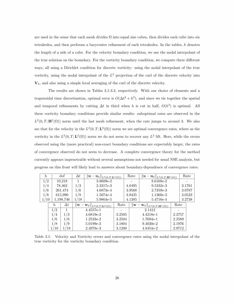
3.1 Velocity and Vorticity errors and convergence rates using the nodal interpolant of thetrue vorticity for the vorticity boundary condition. . . . . . . . . . . . . . . . . . . . 26
3.2 Velocity and Vorticity errors and convergence rates using the nodal interpolant of theL2 projection of the curl of the discrete velocity into Vh, for the vorticity boundarycondition. . . . . . . . . . . . . . . . . . . . . . . . . . . . . . . . . . . . . . . . . . . 27
3.3 Velocity and Vorticity errors and convergence rates using nodal averages of the curlof the discrete velocity for the vorticity boundary condition. . . . . . . . . . . . . . . 27
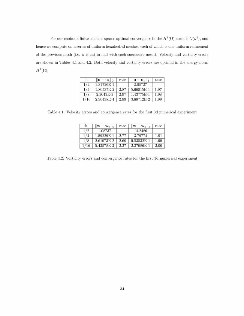
4.1 Velocity errors and convergence rates for the first 3d numerical experiment . . . . . 344.2 Vorticity errors and convergence rates for the first 3d numerical experiment . . . . . 34
3.1 Flow domain for the 3d step test problem. . . . . . . . . . . . . . . . . . . . . . . . . 283.2 Shown above are (top) speed contours and streamlines, (middle) vorticity magnitude,
and (bottom) helical density, from the fine mesh computation at time t = 10 at thex = 5 mid-slice-plane for the 3d step problem with nodal averaging vorticity boundarycondition. . . . . . . . . . . . . . . . . . . . . . . . . . . . . . . . . . . . . . . . . . . 29
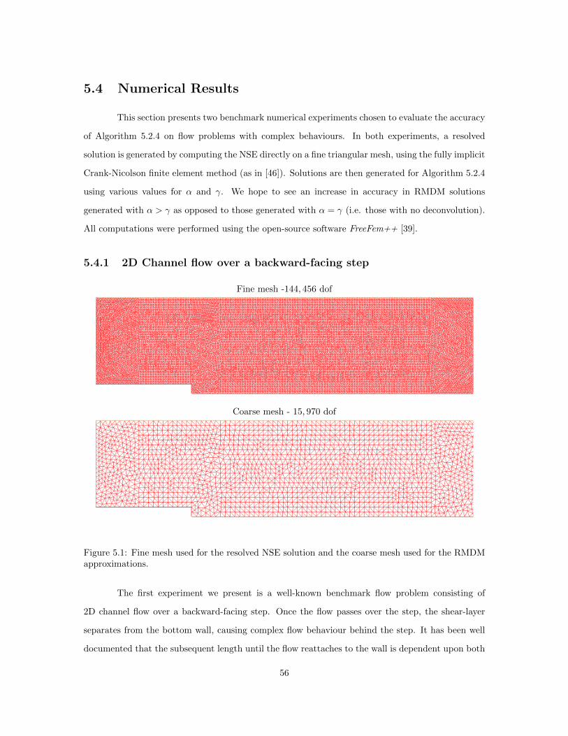
5.1 Fine mesh used for the resolved NSE solution and the coarse mesh used for the RMDMapproximations. . . . . . . . . . . . . . . . . . . . . . . . . . . . . . . . . . . . . . . . 56
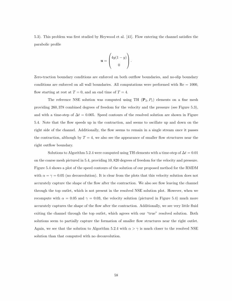
5.2 Fine mesh used for the resolved NSE solution and the coarse mesh used for the RMDMapproximations. . . . . . . . . . . . . . . . . . . . . . . . . . . . . . . . . . . . . . . . 59
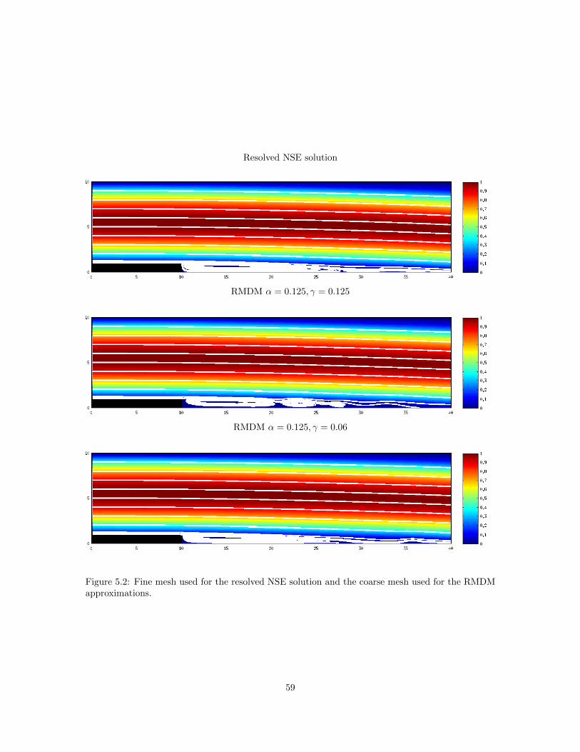
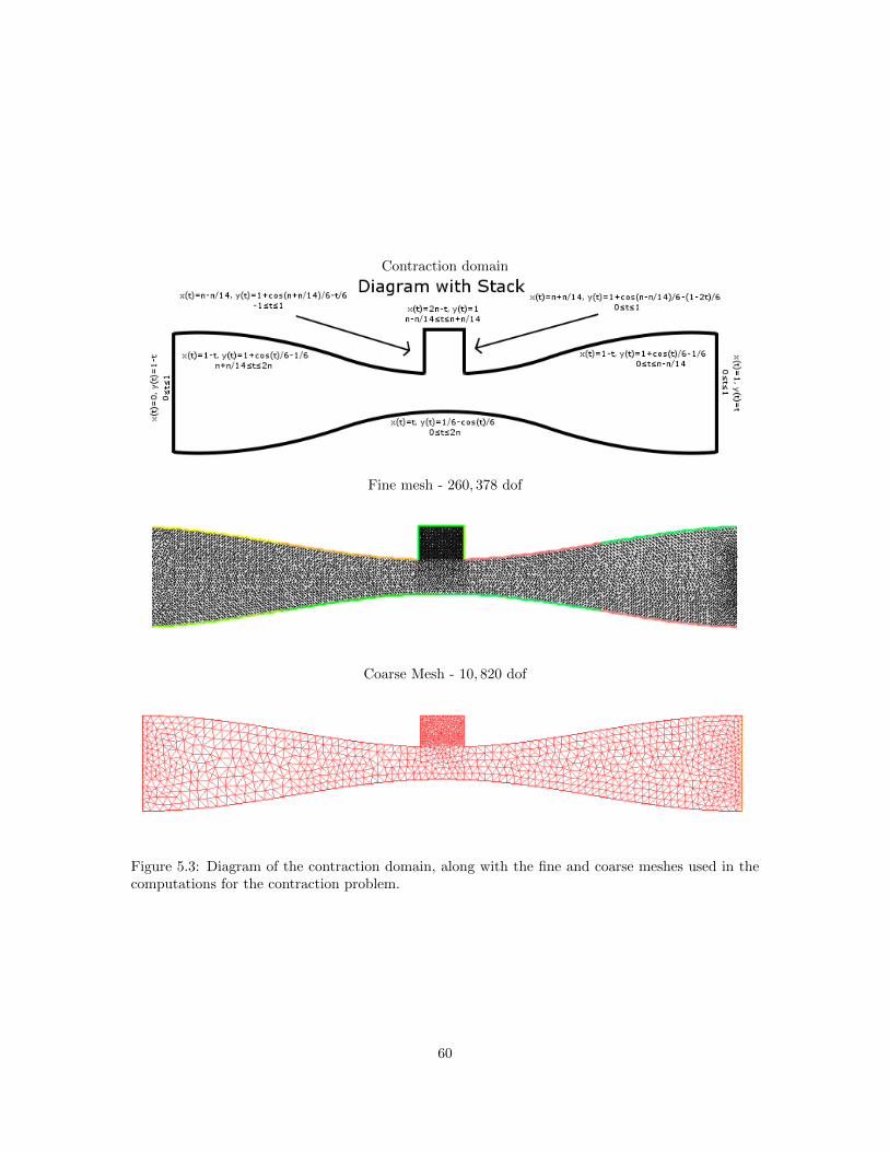
5.3 Diagram of the contraction domain, along with the fine and coarse meshes used inthe computations for the contraction problem. . . . . . . . . . . . . . . . . . . . . . . 60
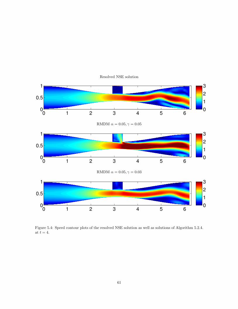
5.4 Speed contour plots of the resolved NSE solution as well as solutions of Algorithm5.2.4. at t = 4. . . . . . . . . . . . . . . . . . . . . . . . . . . . . . . . . . . . . . . . 61
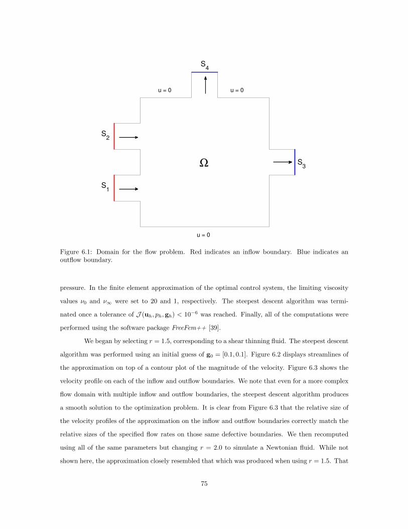
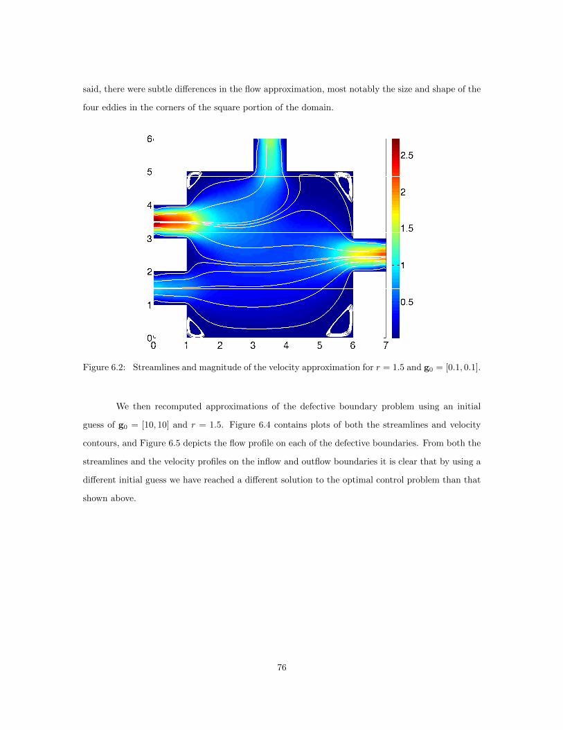
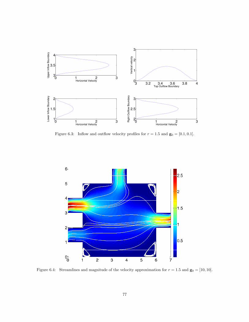
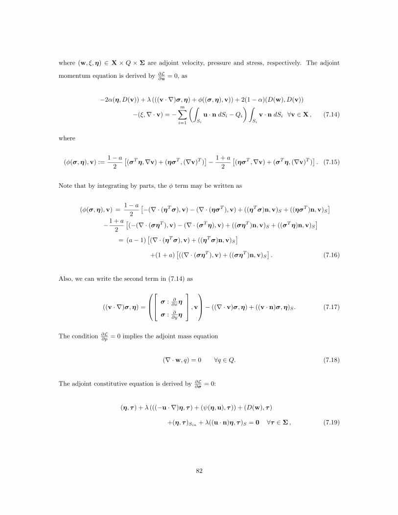
6.2 Streamlines and magnitude of the velocity approximation for r = 1.5 and g0 = [0.1, 0.1]. 766.3 Inflow and outflow velocity profiles for r = 1.5 and g0 = [0.1, 0.1]. . . . . . . . . . . . 776.4 Streamlines and magnitude of the velocity approximation for r = 1.5 and g0 = [10, 10]. 776.5 Inflow and outflow velocity profiles for r = 1.5 and g0 = [10, 10]. . . . . . . . . . . . 78
7.1 Shown above is the domain for the flow problem. . . . . . . . . . . . . . . . . . . . . 917.2 Plots of the magnitude of the velocity and streamlines, velocity and pressure pro-
files on S1, S2, and S3, and stress contours of the solution generated using Dirichletboundary conditions for the velocity and stress. . . . . . . . . . . . . . . . . . . . . . 92
7.3 Plots of the magnitude of the velocity and streamlines, velocity and pressure profileson S1, S2, and S3, and stress contours of the solution generated using the steepestdescent algorithm for the flow rate matching problem with initial guess g = [0.1, ..., 0.1]. 93
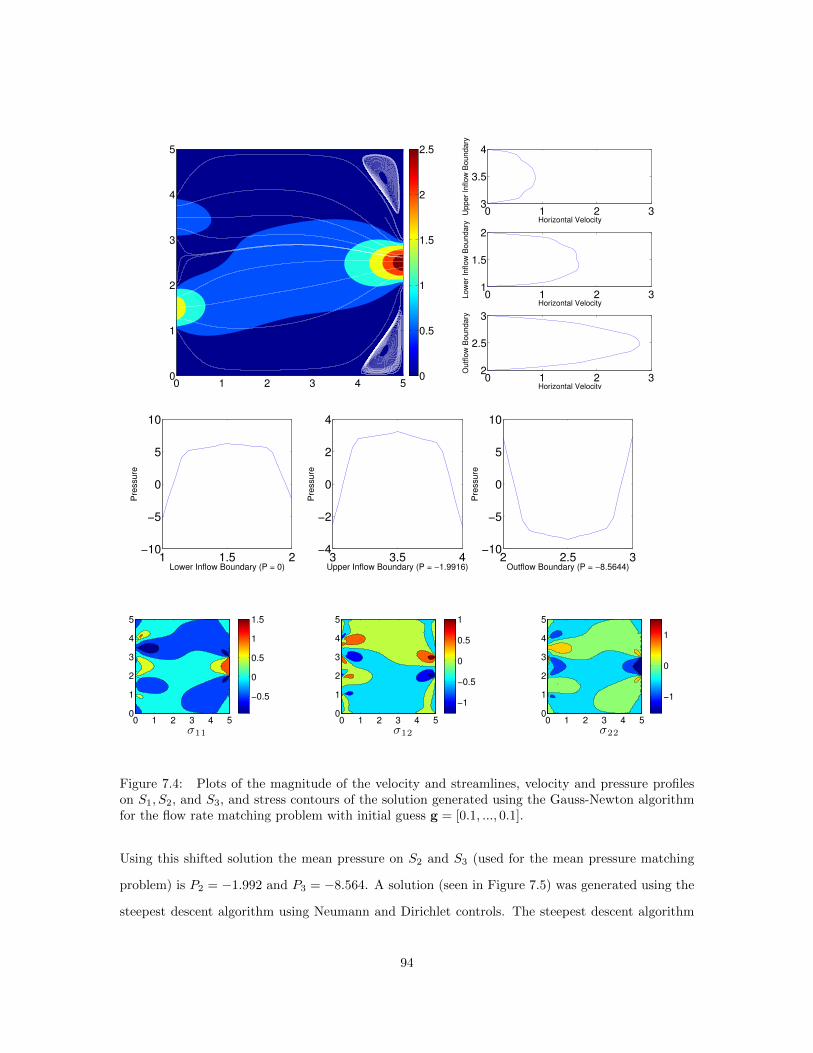
7.4 Plots of the magnitude of the velocity and streamlines, velocity and pressure profileson S1, S2, and S3, and stress contours of the solution generated using the Gauss-Newton algorithm for the flow rate matching problem with initial guess g = [0.1, ..., 0.1]. 94
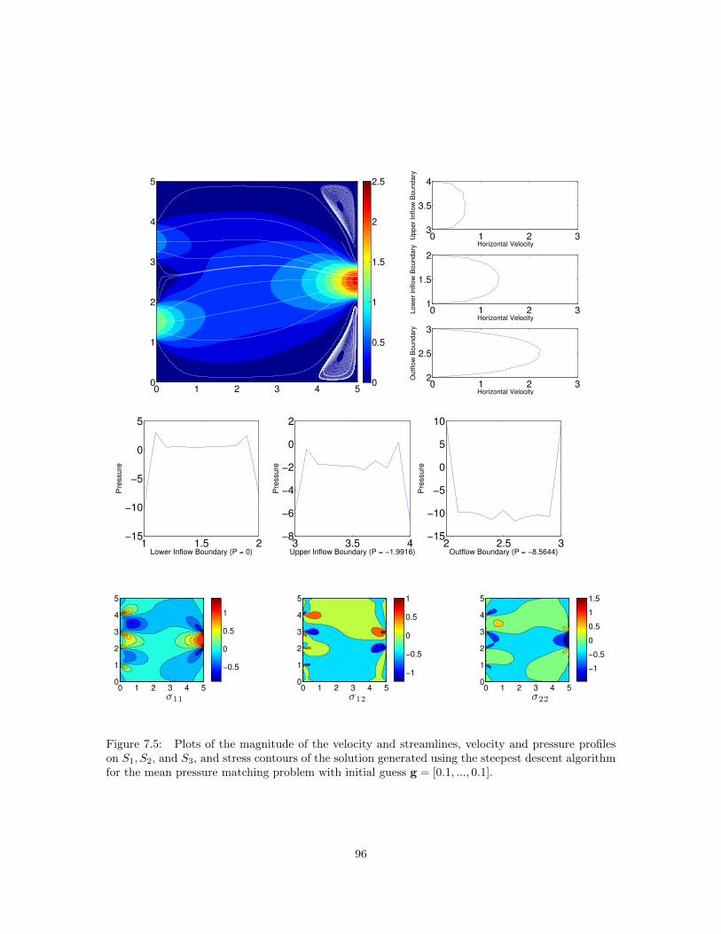
7.5 Plots of the magnitude of the velocity and streamlines, velocity and pressure profileson S1, S2, and S3, and stress contours of the solution generated using the steepestdescent algorithm for the mean pressure matching problem with initial guess g =[0.1, ..., 0.1]. . . . . . . . . . . . . . . . . . . . . . . . . . . . . . . . . . . . . . . . . . 96
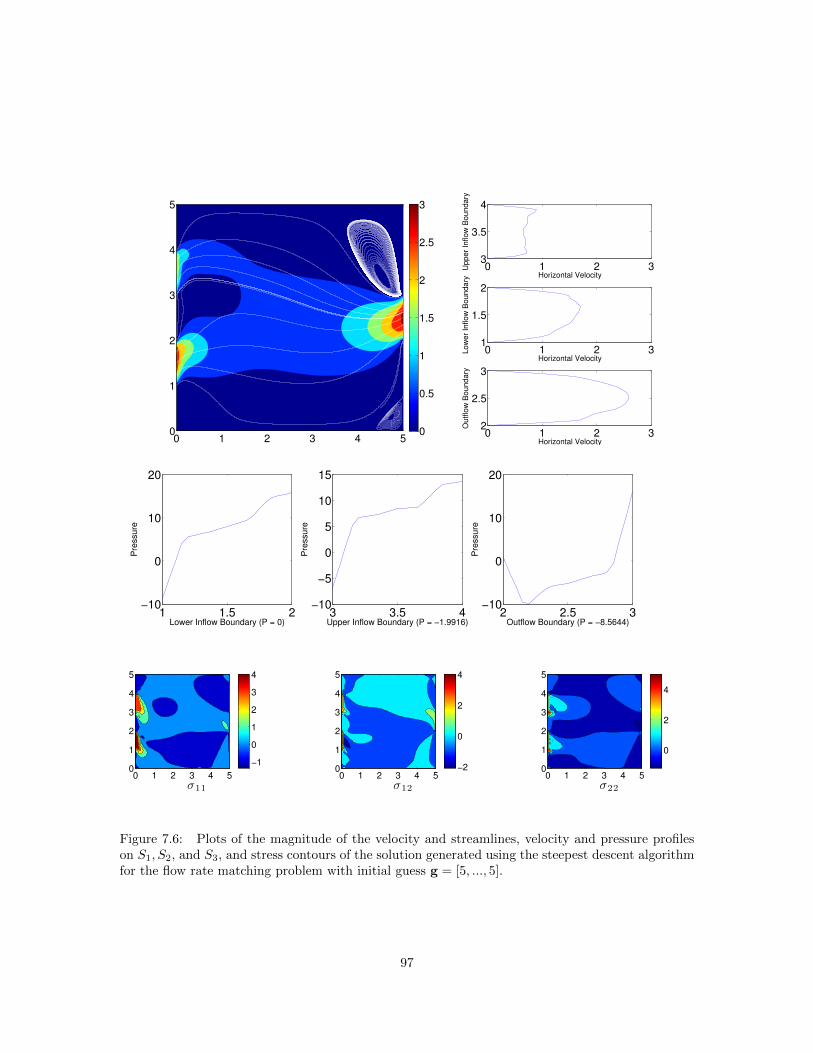
7.6 Plots of the magnitude of the velocity and streamlines, velocity and pressure profileson S1, S2, and S3, and stress contours of the solution generated using the steepestdescent algorithm for the flow rate matching problem with initial guess g = [5, ..., 5]. 97
vii
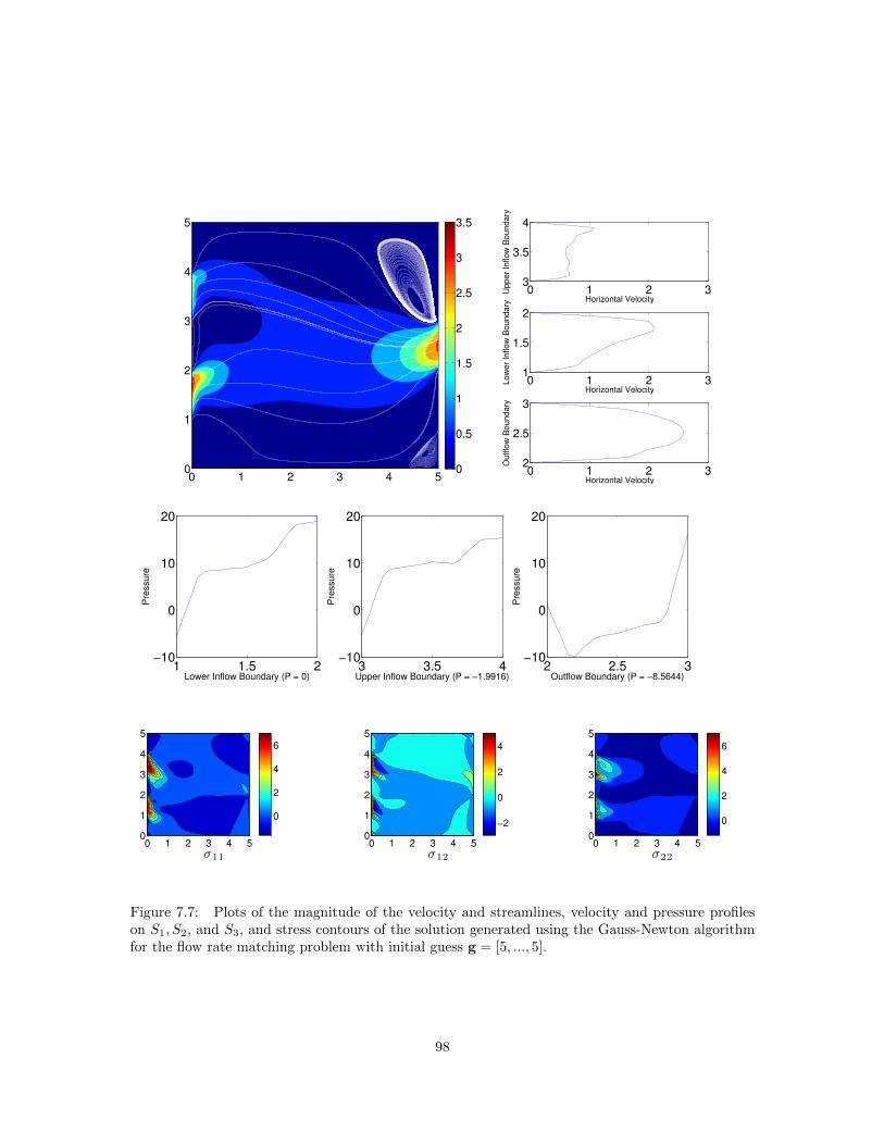
7.7 Plots of the magnitude of the velocity and streamlines, velocity and pressure profileson S1, S2, and S3, and stress contours of the solution generated using the Gauss-Newton algorithm for the flow rate matching problem with initial guess g = [5, ..., 5]. 98
viii
Chapter 1
Introduction
The understanding of fluid flow has been a subject of scientific interest for hundreds of
years. More recently, the branch of fluid mechanics known as computational fluid dynamics (CFD)
has been an area of intense interest for mathematicians due to the multitude of scientific areas that
depend on it. Many industries (e.g. automotive, aerospace, environmental) rely on both accurate
and efficient simulations of various types of fluids. However, state of the art models and methods
are far from being able to efficiently solve most problems of interest in CFD to a desired degree
of precision. Moore’s law states (roughly) that the amount of computing power available doubles
every two years, and has proven to be a fairly accurate estimate over the last 50 years. Despite
the great advances made in computing power in that time period, and even assuming Moore’s law
for computational speed increase continues, the accurate and timely simulation of most flows will
not be achieved in the foreseeable future. Advances in mathematics for CFD have gained far more
towards this goal than computing power, by developing robust and efficient algorithms built on solid
mathematical and physical grounds.
It is the goal of this work to extend the state of the art in mathematics of CFD for two
important problems. The first concerns the accurate and efficient simulation of incompressible,
viscous Newtonian fluids. We will present and analyze a new numerical method for approximating
solutions to the velocity-vorticity-helicity formulation of the Navier-Stokes equations. The driving
force behind this new method is that it offers increased physical fidelity and numerical accuracy,
along with a step towards further understanding the important but ill-understood physical quantity
helicity. Discussion of this method naturally raises the very difficult question of how to accurately
1
impose boundary conditions on the vorticity, as well as how to compute with turbulent flows. For
the former, we propose a new natural boundary condition for the vorticity equation which increases
both the accuracy and physical relevance of our discrete vorticity approximation. For the latter, we
consider a new reduced-order multiscale model for simulating Newtonian fluids.
The second main problem we study in this work concerns the robust simulation of non-
Newtonian fluids in the absence of standard boundary conditions. This problem often arises when
modeling flow in an unbounded domain (e.g. modeling blood flow in a portion of a blood vessel). We
consider two different approaches for developing accurate and efficient methods for these “defective-
boundary” problems for non-Newtonian flows. The first, a gradient-descent method, is presented
and tested for both generalized-Newtonian and viscoelastic flow models, and analyzed in the case of
the former. The second, a nonlinear least squares method, is presented and tested on a viscoelastic
flow model.
The flow of time-dependent, incompressible, viscous Newtonian flows is modeled by the
Navier-Stokes equations (NSE), which may be derived from the continuity equation (describing
conservation of mass) and the equation describing conservation of momentum. In dimensionless
form, the NSE are formulated as
∂u
∂t− ν∆u + u · ∇u +∇p = f , (1.1)
∇ · u = 0, (1.2)
where u and p denote the fluid velocity and pressure, respectively, f denotes an external body force,
and ν > 0 denotes the fluid’s kinematic viscosity. The Reynolds number Re = ν−1 is a dimensionless
parameter representing the ratio of inertial forces to viscous forces. In laminar flows, which are
characterized by low Reynolds number, viscous forces dominate inertial forces, making the flow
field smooth. Simulations of laminar flows can often be performed without too much complication.
For flows with moderate Reynolds numbers, inertial forces start to play a larger role, resulting in
complex flow behaviors, making predictions much more difficult. Turbulent flows, characterized by
high Reynolds numbers, present very complex and chaotic flow properties, often requiring special
models and methods.
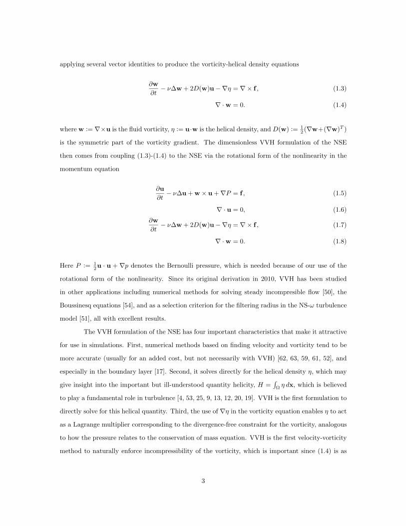
In 2010, a velocity-vorticity-helicity (VVH) formulation of the NSE was presented in [55].
This formulation was derived by taking the curl of mass and momentum equations (1.1)-(1.2), and
2
applying several vector identities to produce the vorticity-helical density equations
∂w
∂t− ν∆w + 2D(w)u−∇η = ∇× f , (1.3)
∇ ·w = 0. (1.4)
where w := ∇×u is the fluid vorticity, η := u·w is the helical density, and D(w) := 12 (∇w+(∇w)T )
is the symmetric part of the vorticity gradient. The dimensionless VVH formulation of the NSE
then comes from coupling (1.3)-(1.4) to the NSE via the rotational form of the nonlinearity in the
momentum equation
∂u
∂t− ν∆u + w × u +∇P = f , (1.5)
∇ · u = 0, (1.6)
∂w
∂t− ν∆w + 2D(w)u−∇η = ∇× f , (1.7)
∇ ·w = 0. (1.8)
Here P := 12u · u + ∇p denotes the Bernoulli pressure, which is needed because of our use of the
rotational form of the nonlinearity. Since its original derivation in 2010, VVH has been studied
in other applications including numerical methods for solving steady incompresible flow [50], the
Boussinesq equations [54], and as a selection criterion for the filtering radius in the NS-ω turbulence
model [51], all with excellent results.
The VVH formulation of the NSE has four important characteristics that make it attractive
for use in simulations. First, numerical methods based on finding velocity and vorticity tend to be
more accurate (usually for an added cost, but not necessarily with VVH) [62, 63, 59, 61, 52], and
especially in the boundary layer [17]. Second, it solves directly for the helical density η, which may
give insight into the important but ill-understood quantity helicity, H =∫
Ωη dx, which is believed
to play a fundamental role in turbulence [4, 53, 25, 9, 13, 12, 20, 19]. VVH is the first formulation to
directly solve for this helical quantity. Third, the use of ∇η in the vorticity equation enables η to act
as a Lagrange multiplier corresponding to the divergence-free constraint for the vorticity, analogous
to how the pressure relates to the conservation of mass equation. VVH is the first velocity-vorticity
method to naturally enforce incompressibility of the vorticity, which is important since (1.4) is as
3
much a mathematical constraint as it is a physical one, making its violation inconsistent on multiple
levels. Finally, the structure of the VVH system allows for a natural splitting of the system into a
two-step linearization, since lagging vorticity in the velocity equation linearizes the equation, and
similarly lagging velocity in the vorticity equation linearizes this equation as well. A numerical
method based on such a splitting was proposed in [55], and when coupled with a finite element
discretization, was shown to be accurate on some simple test problems. Chapter 3 of this work
will precisely define and further study this discretization of the VVH formulation of the NSE by
providing a rigorous stability analysis (for both velocity and vorticity), and testing the method on
a benchmark problem.
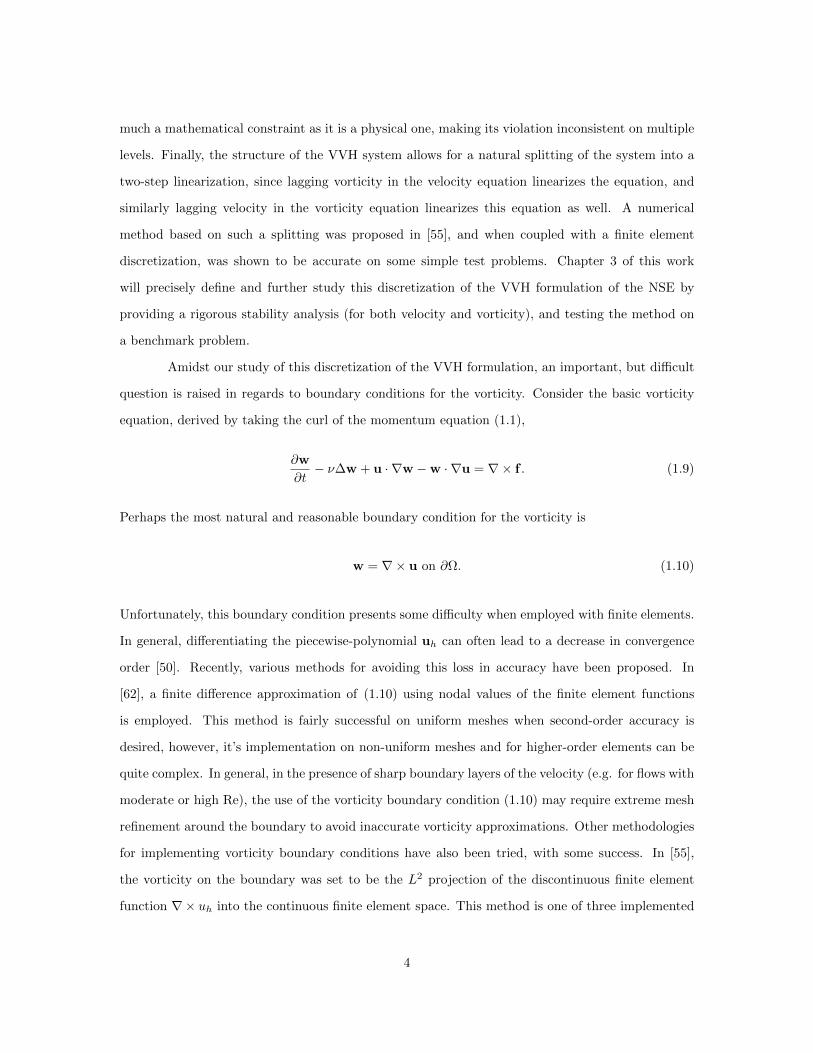
Amidst our study of this discretization of the VVH formulation, an important, but difficult
question is raised in regards to boundary conditions for the vorticity. Consider the basic vorticity
equation, derived by taking the curl of the momentum equation (1.1),
∂w
∂t− ν∆w + u · ∇w −w · ∇u = ∇× f . (1.9)
Perhaps the most natural and reasonable boundary condition for the vorticity is
w = ∇× u on ∂Ω. (1.10)
Unfortunately, this boundary condition presents some difficulty when employed with finite elements.
In general, differentiating the piecewise-polynomial uh can often lead to a decrease in convergence
order [50]. Recently, various methods for avoiding this loss in accuracy have been proposed. In
[62], a finite difference approximation of (1.10) using nodal values of the finite element functions
is employed. This method is fairly successful on uniform meshes when second-order accuracy is
desired, however, it’s implementation on non-uniform meshes and for higher-order elements can be
quite complex. In general, in the presence of sharp boundary layers of the velocity (e.g. for flows with
moderate or high Re), the use of the vorticity boundary condition (1.10) may require extreme mesh
refinement around the boundary to avoid inaccurate vorticity approximations. Other methodologies
for implementing vorticity boundary conditions have also been tried, with some success. In [55],
the vorticity on the boundary was set to be the L2 projection of the discontinuous finite element
function ∇× uh into the continuous finite element space. This method is one of three implemented
4
in the numerical testing of our method for the VVH system presented in Chapter 3, providing fairly
accurate results on a benchmark flow problem. Other strategies include using the boundary element
method [42], or the lattice Boltzmann method [18]. In Chapter 4, we employ a different approach
in deriving a new vorticity boundary condition, in hopes of avoiding any unnecessary complication.
The proposed method includes natural boundary conditions for a weak formulation of the vorticity
equation. The boundary conditions are derived directly from the physical equations and the finite
element method, making them simpler to understand than some of the aforementioned strategies.
A full derivation of these vorticity boundary conditions will be presented in Chapter 4, along with
a numerical scheme to evaluate their effectiveness in a numerical experiment.
Another clear need in the development of the VVH algorithm is for some kind of stabiliza-
tion/subgrid model to allow us to handle higher Re flows. In Chapter 5 we consider a new reduced
order, multiscale, approximate deconvolution model for Newtonian flows. Approximate deconvo-
lution models (ADM) are a form of large eddy simulation (LES) models introduced in [2, 3] for
the purpose of simulating large-scale flow strctures at a reduced computational cost compared with
direct numerical simulation (DNS). We know from Kolmogorov’s 1941 theory that eddies below a
critical size (O(Re−3/4) for 3d flow) are dominated by viscous forces and disappear very quickly,
while those above this critical size are deterministic in nature. Hence, a DNS requires O(Re9/4)
mesh points in space per time step to accurately simulate eddies in 3d. Even for moderate Re flows,
this requirement makes DNS computationally infeasible. ADM models (and LES models in general)
aim to avoid this problem by filtering out small scales, while modeling their effect on the large scales.
Because only large scales are being solved for, these models require a significantly smaller amount
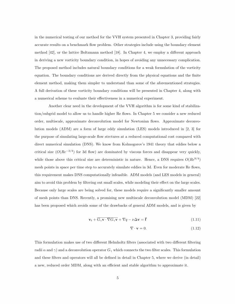
of mesh points than DNS. Recently, a promising new multiscale deconvolution model (MDM) [22]
has been proposed which avoids some of the drawbacks of general ADM models, and is given by
vt +Gγv · ∇Gγv +∇q − ν∆v = f (1.11)
∇ · v = 0. (1.12)
This formulation makes use of two different Helmholtz filters (associated with two different filtering
radii α and γ) and a deconvolution operator Gγ which connects the two filter scales. This formulation
and these filters and operators will all be defined in detail in Chapter 5, where we derive (in detail)
a new, reduced order MDM, along with an efficient and stable algorithm to approximate it.
5
The second half of this work is concerned with the accurate and efficient simulation of the
defective boundary problem for two types of non-Newtonian fluids. The modeling of flow in an
unbounded domain requires the introduction of artificial boundaries. Often, the flow is assumed to
satisfy some Dirichlet or Neumann boundary condition on a portion of these artificial boundaries
(e.g. inflow or outflow boundaries). However, the amount of boundary data available for a given
flow is often very limited, making these types of boundary conditions very hard to impose. In many
practical applications the only flow data available are quantitative (e.g. average flow rates, mean
pressure values, etc.). In situations like these, it is often more realistic to model the flow using
defective boundary conditions. Typically, governing equations are chosen depending on the flow
being modeled, and instead of completing these equations with standard Dirichlet or Neumann type
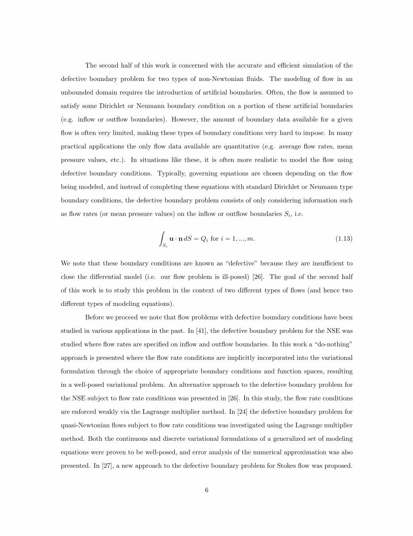
boundary conditions, the defective boundary problem consists of only considering information such
as flow rates (or mean pressure values) on the inflow or outflow boundaries Si, i.e.
∫Si
u · n dS = Qi for i = 1, ...,m. (1.13)
We note that these boundary conditions are known as “defective” because they are insufficient to
close the differential model (i.e. our flow problem is ill-posed) [26]. The goal of the second half
of this work is to study this problem in the context of two different types of flows (and hence two
different types of modeling equations).
Before we proceed we note that flow problems with defective boundary conditions have been
studied in various applications in the past. In [41], the defective boundary problem for the NSE was
studied where flow rates are specified on inflow and outflow boundaries. In this work a “do-nothing”
approach is presented where the flow rate conditions are implicitly incorporated into the variational
formulation through the choice of appropriate boundary conditions and function spaces, resulting
in a well-posed variational problem. An alternative approach to the defective boundary problem for
the NSE subject to flow rate conditions was presented in [26]. In this study, the flow rate conditions
are enforced weakly via the Lagrange multiplier method. In [24] the defective boundary problem for
quasi-Newtonian flows subject to flow rate conditions was investigated using the Lagrange multiplier
method. Both the continuous and discrete variational formulations of a generalized set of modeling
equations were proven to be well-posed, and error analysis of the numerical approximation was also
presented. In [27], a new approach to the defective boundary problem for Stokes flow was proposed.
6
This approach formulates the defective boundary problem as an optimal control problem through the
choice of a suitable functional to minimize. This approach proved to be versatile, as the functional to
minimize can be altered to match various kinds of defective boundaries (flow rates, mean pressure,
etc). In the optimal control formulation, the control was chosen to be a constant normal stress
on each of the inflow and outflow boundaries, and appears in the modeling equations through the
addition of a boundary integral (often referred to as a “boundary control” [35]).
The study of optimal control problems for Newtonian and non-Newtonian fluids has been
istelf an active research area in the recent past, e.g. [35, 36, 37]. One approach to solve these types
of optimization problems is based off of solving “sensitivity equations,” which are derived through
the Frechet derivative of the constraint operator with respect to the control variables [35, 11, 38].
An alternative approach studied in [35, 49] is an adjoint-based optimization method, in which the
method of Lagrange multipliers is used to derive an optimality system consisting of constraint equa-
tions, adjoint equations, and a necessary condition. In [21] an optimal control problem for the
Ladyzhenskaya model for generalized-Newtonian flows was studied. Additionally, a shape optimiza-
tion problem for blood flow modeled by the Cross model was presented in [1]. In [48] a defective
boundary problem for generalized-Newtonian flows was studied. In that work the model problem
considered was the three-field power law model subject to flow rate or mean pressure conditions on
portions of the boundary. The defective boundary problem was formulated as an optimal control
problem which was then transformed into an unconstrained optimization problem via the Lagrange
multiplier method. However, analysis of the adjoint problem and the method of Lagrange multipliers
was limited, in part due to the choice of modeling equations.
In Chapter 6, we begin by considering the defective boundary problem for generalized-
Newtonian fluids governed by the Cross modeling equations [16] (which will be explicitly defined
later in this work). Newtonian fluids are characterized by having a shear stress, denoted by σ, that
is directly proportional to its shear rate (given by D(u)), i.e.
σ = 2νD(u), (1.14)
where the fluid viscosity ν is constant. On the other hand, generalized-Newtonian flows have the
same stress-strain relationship, but with a non-constant fluid viscosity dependent upon the velocity
7
of the flow
σ = 2ν(|D(u)|)D(u), (1.15)
where the viscosity function ν(|D(u)|) is chosen to reflect the flow being modeled. The Cross model
specifies the viscosity function as
ν(|D(u)|) := ν∞ +(ν0 − ν∞)
1 + (λ|D(u)|)2−r , (1.16)
where λ > 0 is a time constant, 1 ≤ r ≤ 2 is a dimensionless rate constant, and ν0 and ν∞
denote limiting viscosity values at a zero and infinite shear rate, respectively, assumed to satisfy
0 ≤ ν∞ ≤ ν0. We take the approach of [48] to approximate our model problem subject to flow
rate and mean pressure conditions. The problem is formulated as an optimal control problem for
which we analytically justify the use of the method of Lagrange multipliers to derive an optimality
system. We then show that the resulting adjoint system is well-posed. Finally, we consider a complex
numerical experiment to test the robustness of an optimization algorithm previously presented in
[48].
In Chapter 7, we consider the same defective boundary problem but for viscoelastic flu-
ids governed by the Johnson-Segalman modeling equations. Viscoelastic fluids are a type of non-
Newtonian fluid that exhibit both viscous and elastic characteristics when undergoing deformation.
This is reflected in the modeling equations by an extra nonlinear constitutive equation, which relates
the stress tensor σ to the fluid velocity. Some analytical and numerical studies for an optimal control
of non-Newtonian flows can be found in [1, 21, 45, 49]. The Johnson-Segalman modeling equations
for viscoelastic, creeping flow are given by
σ + λ(u · ∇)σ + λga(σ,∇u)− 2αD(u) = 0, (1.17)
−∇ · σ − 2(1− α)∇ ·D(u) +∇p = f , (1.18)
∇ · u = 0. (1.19)
Here λ denotes the Weissenberg number, defined as the product of relaxation time and a characteris-
tic strain rate of the fluid, α is a number satisfying 0 < α < 1 which can be considered as the fraction
8
of viscoelastic viscosity, and ga(σ,∇u) is a nonlinear function of σ and u that will be explicitly de-
fined in Chapter 7. We consider the defective boundary problem for viscoelastic fluids governed by
these equations. This includes a fully detailed formulation of the problem itself, the minimization
problem, and a derivation of the optimality system. The numerical algorithm presented in Chapter
6 will then be used to solve the minimization problem, along with a second, new algorithm. Finally,
we consider a numerical test to compare and contrast both algorithms.
This work is arranged as follows. Chapter 2 contains mathematical notation and prelimi-
naries that will be used throughout the following sections. Chapter 3 presents a stability analysis
and numerical testing of a finite element method for the VVH formulation. Chapter 4 fully defines a
new vorticity boundary condition, and presents a numerical experiment designed to verify its accu-
racy. Chapter 5 derives and analyzes a new reduced order MDM, and presents two numerical tests
to verify its efficiency. Chapter 6 presents the work on generalized-Newtonian flows with defective
boundary conditions, and Chapter 7 contains the work on viscoelastic flows with defective boundary
conditions. Finally, Chapter 8 contains conclusions from the various works presented herein.
9
Chapter 2
Preliminaries
Throughout the analysis presented in this work we will assume that the domain Ω denotes
a bounded, connected subset of Rd (with d = 2 or 3), with piecewise smooth boundary ∂Ω. We will
denote the L2(Ω) norm and inner product by ‖·‖ and (·, ·), respectively, while Lp(Ω) norms will be
denoted by ‖·‖Lp . Sobolev W kp (Ω) norms and seminorms will be indicated by ‖·‖Wk
pand | · |Wp
k,
respectively. We will use the standard notation of Hk(Ω) to refer to the sobolev space W k2 (Ω), with
norm ‖·‖k. Dual spaces will be denoted (·)∗ with duality pairing 〈·, ·〉 and norm ‖·‖∗. For domains
other than Ω we will explicitly indicate the domain in the space and norm notation. For k ∈ R the
space Hk0 is defined as
Hk0 (Ω) := v ∈ Hk(Ω) | v = 0 on ∂Ω.
The zero-mean subspace of L2(Ω) is defined as
L20(Ω) := q ∈ L2(Ω) |
∫Ω
q = 0.
For functions v(x, t) defined on Ω × (0, T ) for some positive end time T , we will make use
of the norms
‖v‖n,k :=
(∫ T
0
‖v(·, t)‖nk dt
)1/n
and ‖v‖∞,k := ess sup0<t<T
‖v(·, t)‖k .
For functions of time, we will use the notation tn := n∆t where ∆t denotes a chosen time-step. For
10
continuous functions of time f(t), we use the notation
fn := f(tn),
and
fn+1/2 := f(tn+ 12 ) = f
(tn+1 + tn
2
).
The average of the nth and (n+ 1)st time level of a discrete function v is denoted
vn+1/2 :=vn+1 + vn
2.
Our error analysis will require the use of discrete time analogues of the continuous in time norms:
‖|v|‖p,k :=
(NT∑n=1
‖vn‖pk ∆t
)1/p
and ‖|v|‖∞,k := max1≤n≤NT
‖vn‖k
We will use bold font to denote vector functions and tensor functions. We will also use bold
font to denote vector function spaces, e.g.
H1(Ω) := (H1(Ω))d and H10(Ω) := (H1
0 (Ω))d.
Throughout our analysis we will frequently employ the following inequality, one result of
which is that for v ∈ H10 (Ω), the seminorm |v|1 is equivalent to ‖v‖1.
Lemma 2.0.1 (The Poincare-Friedrichs inequality). There exists a positive constant CPF = CPF (Ω)
such that
‖v‖ ≤ CPF ‖∇v‖ ∀ v ∈ H10 (Ω).
Proof. A proof of this well known inequality can be found in [28].
We will often use the (H10 (Ω))∗ = H−1(Ω) norm, denoted by ‖·‖−1, to measure the size of
11
a forcing function. The H−1(Ω) norm is defined as
‖f‖−1 := supv∈H1
0 (Ω)
〈f, v〉‖∇v‖
.
We note that the space H−1(Ω) is the closure of L2(Ω) in ‖·‖−1.
The continuous velocity, pressure, and stress spaces, denoted X, Q, and Σ, respectively, will
be specified in each chapter. The weakly divergence-free subspace V of X is defined as
V := v ∈ X | (∇ · v, q) = 0 ∀ q ∈ Q.
In the discrete setting, we begin by letting τh denote a regular, conforming triangulation or
tetrahedralization of Ω. The velocity and pressure finite element spaces defined on τh will be denoted
as Xh and Qh, respectively, and will be specified in each chapter. The divergence-free subspace Vh
of Xh is defined as
Vh := vh ∈ Xh | (∇ · vh, qh) = 0∀ qh ∈ Qh.
We will often make use of the Taylor-Hood (TH) element pair, defined as (Xh, Qh) =
Table 3.3: Velocity and Vorticity errors and convergence rates using nodal averages of the curl ofthe discrete velocity for the vorticity boundary condition.
27
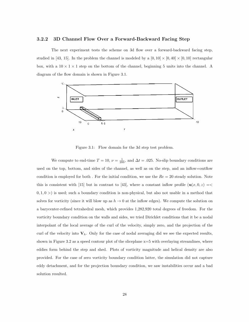
3.2.2 3D Channel Flow Over a Forward-Backward Facing Step
The next experiment tests the scheme on 3d flow over a forward-backward facing step,
studied in [43, 15]. In the problem the channel is modeled by a [0, 10]× [0, 40]× [0, 10] rectangular
box, with a 10 × 1 × 1 step on the bottom of the channel, beginning 5 units into the channel. A
diagram of the flow domain is shown in Figure 3.1.
Figure 3.1: Flow domain for the 3d step test problem.
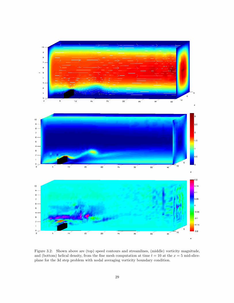
We compute to end-time T = 10, ν = 1200 , and ∆t = .025. No-slip boundary conditions are
used on the top, bottom, and sides of the channel, as well as on the step, and an inflow=outflow
condition is employed for both . For the initial condition, we use the Re = 20 steady solution. Note
this is consistent with [15] but in contrast to [43], where a constant inflow profile (u(x, 0, z) =<
0, 1, 0 >) is used; such a boundary condition is non-physical, but also not usable in a method that
solves for vorticity (since it will blow up as h→ 0 at the inflow edges). We compute the solution on
a barycenter-refined tetrahedral mesh, which provides 1,282,920 total degrees of freedom. For the
vorticity boundary condition on the walls and sides, we tried Dirichlet conditions that it be a nodal
interpolant of the local average of the curl of the velocity, simply zero, and the projection of the
curl of the velocity into Vh. Only for the case of nodal averaging did we see the expected results,
shown in Figure 3.2 as a speed contour plot of the sliceplane x=5 with overlaying streamlines, where
eddies form behind the step and shed. Plots of vorticity magnitude and helical density are also
provided. For the case of zero vorticity boundary condition latter, the simulation did not capture
eddy detachment, and for the projection boundary condition, we saw instabilities occur and a bad
solution resulted.
28
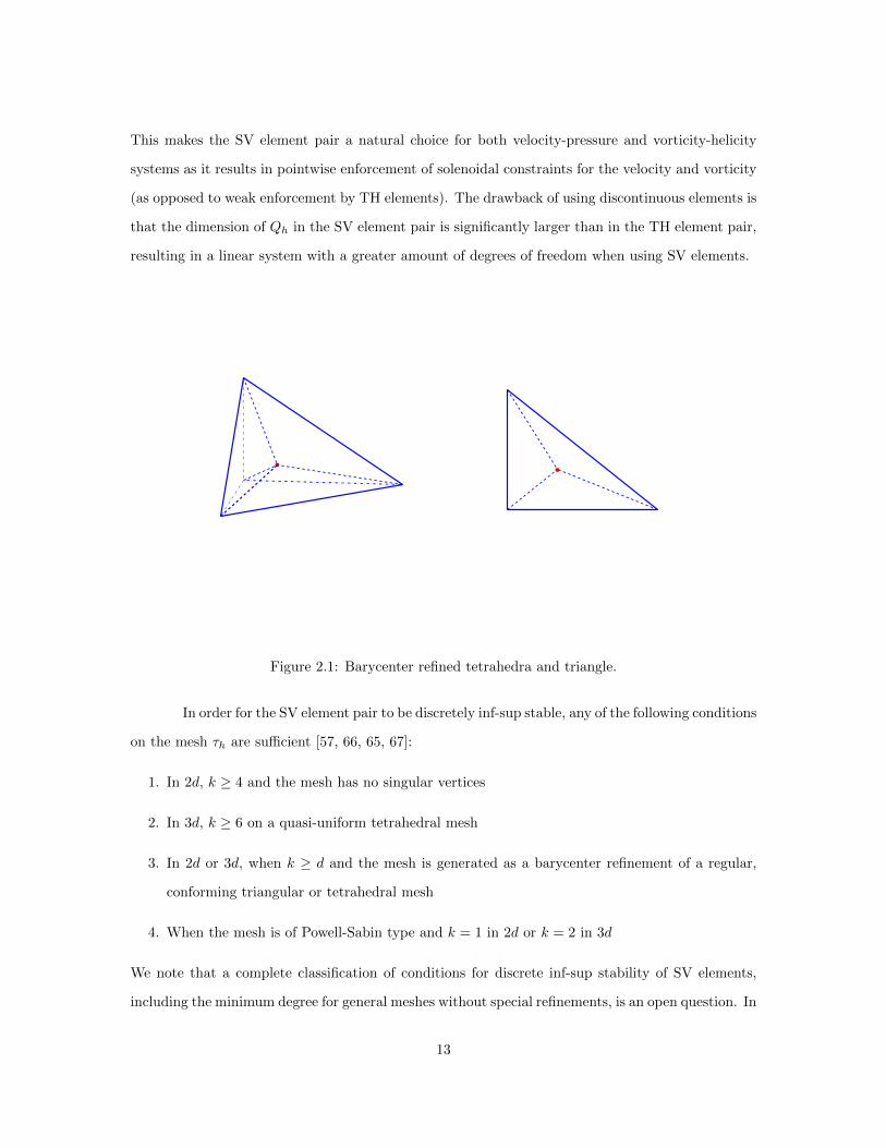
Figure 3.2: Shown above are (top) speed contours and streamlines, (middle) vorticity magnitude,and (bottom) helical density, from the fine mesh computation at time t = 10 at the x = 5 mid-slice-plane for the 3d step problem with nodal averaging vorticity boundary condition.
29
Chapter 4
Natural vorticity boundary
conditions for coupled vorticity
equations
This chapter derives new natural boundary conditions for the vorticity equations that result
from the application of the curl operator to the steady NSE momentum equation, given by
−ν∆w + (u · ∇)w − (w · ∇)u = ∇× f . (4.1)
A finite element method for solving the 3d vorticity equations is presented to test the accuracy of
the proposed boundary conditions, and results from a simple numerical experiment are presented
verifying optimal convergence rates are acheived. We note that the vorticity boundary conditions
presented herein could also easily be derived for the time-dependent vorticity equations, and would
apply equally well to the vorticity-helical density equations studied in the previous chapter.
4.1 Derivation
Suppose we are given some general Dirichlet boundary condition for the velocity in the NSE,
i.e. u = g on ∂Ω. We are mainly interested in the case where ∂Ω is a solid wall with no-slip (g = 0)
30
boundary conditions, and so leaving g to be general includes this case. Our first vorticity boundary
condition easily follows:
w · n = (∇× g) · n on ∂Ω. (4.2)
To deduce two more boundary conditions for w, consider the incompressible NSE written in rota-
tional form (see, e.g. [32] for more on rotational form of NSE),
ν∇×w + w × u +∇P = f ,
where P = 12 |u|
2 + p is the Bernoulli pressure. Taking the tangential component of both sides of
this equation gives
ν(∇×w)× n = (f −∇P −w × g)× n on ∂Ω, (4.3)
which provides two more boundary conditions for w in terms of the primitive NSE velocity and
pressure variables. In velocity-vorticity splitting schemes where the NSE momentum equation is
used for the velocity (as in the work of Wong and Baker [62] or the scheme presented in the previous
chapter of this work), the NSE velocity and pressure are considered as knowns when solving the
Again, (u,σ) in (7.26)-(7.28) is the solution of (7.9)–(7.11) with g replaced by g. Note that taking
(v, q, τ ) = (z, ϕ, t) in (7.23)-(7.25), (v, q, τ ) = (w, ξ,η) in (7.26)-(7.28) and using integration by
parts, (7.15), (7.17) and (7.20), we can show
m∑i=1
yi
∫Si
w · n dS = (hN , z)S + (hD, t)Sin,
thereforeN ′(g)
hN
hD
,
y
γ
β
=
m∑i=1
yi
∫Si
w · n dS +√ε1(hN ,γ)S +
√ε2(hD,β)Sin
= (hN , z)S + (hD, t)Sin +√ε1(hN ,γ)S +
√ε2(hD,β)Sin
=
hN
hD
, (N ′(g))∗
y
γ
β
. (7.29)
We adopt the following basic conjugate gradient algorithm for the linear least squares prob-
lem (7.22), which can be found in many references. For example, see [31] or [33]. For the algorithm,
we adopt the notation A = N ′(g), b = −N(g), and x = h.
Algorithm 7.5.1. (Conjugate Gradient Method for the Least Squares Problem)
Given A, b, and x(0),
1. Set r(0) = b−Ax(0),
p(0) = A∗r(0).
2. For n = 0, 1, 2, · · · ,
89
a. if ‖A∗r(n)‖GN×GD< ε stop,
b. σ(n) = ‖A∗r(n)‖2GN×GD/‖Ap(n)‖2Rm×GN×GD
,
c. x(n+1) = x(n) + σ(n)p(n),
d. r(n+1) = r(n) − σ(n)Ap(n),
e. τ (n) = ‖A∗r(n+1)‖2GN×GD/‖A∗r(n)‖2GN×GD
,
f. p(n+1) = A∗r(n+1) + τ (n)p(n).
Thus, the nonlinear least squares problem (7.21) can be solved using the following Gauss-
Newton algorithm.
Algorithm 7.5.2.
1. Choose g(0).
2. For n = 1, 2, 3, . . .,
a. compute h(n) by the conjugate gradient algorithm 7.5.1 with A = N ′(g(n−1)), b = −N(g(n−1)),
and x = h(n);
b. set g(n) = g(n−1) + h(n).
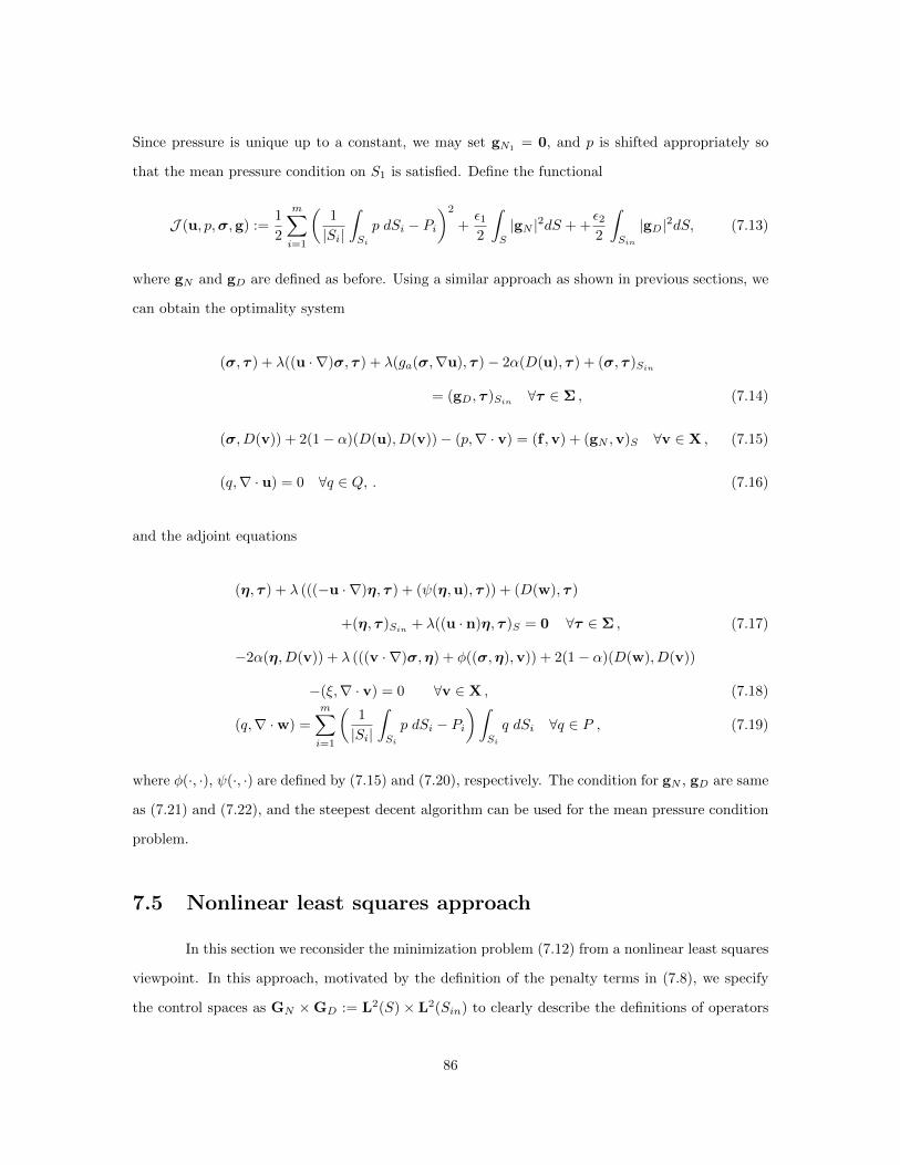
7.6 Numerical Results
In this section we consider a model flow problem subject to specified flow rate or mean
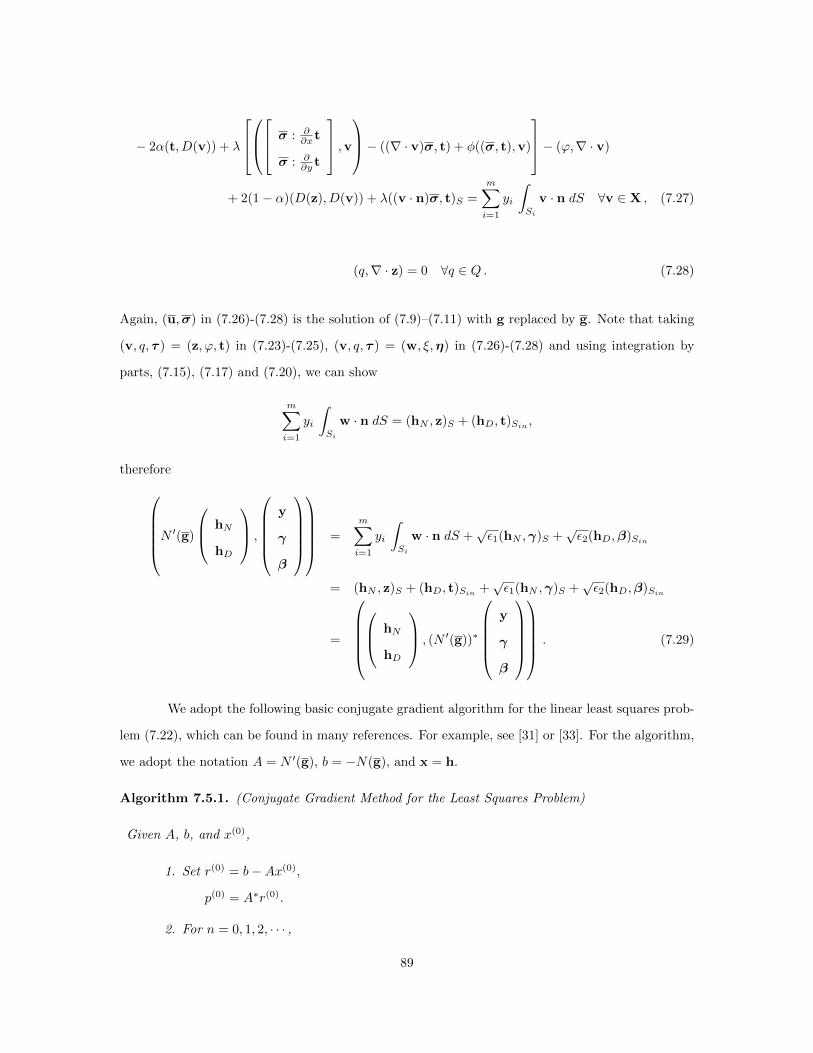
pressure conditions on defective boundaries. Consider the problem of flow in a square domain,
Ω = (0, 5) × (0, 5), containing three defective boundaries S1 = (x, y) : x = 0, 1 < y < 2, S2 =
(x, y) : x = 0, 3 < y < 4, and S3 = (x, y) : x = 5, 2 < y < 3 (as seen in Figure 7.1). In the model
equations (7.1)-(7.3) we take the parameters λ = 0.5, α = 0.5, and a = 0. In the steepest descent
algorithm the golden section search method was used to determine the optimal step sizes in both the
flow rate and mean pressure matching problems. Computations were performed on both 30×30 and
50× 50 triangular meshes, providing 29,058 and 79,856 total degrees of freedom, respectively. In all
tests, the results on the different meshes provided identical plots. All computations were performed
using the software FreeFem++ [39] on a Macbook Pro with 2.26 GHz Intel Core 2 Duo CPU and
2GB of 1066MHz DDR3 SDRAM.
90
Ω S3
S2
S1
u=0
u=0
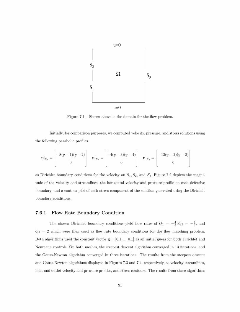
Figure 7.1: Shown above is the domain for the flow problem.
Initially, for comparison purposes, we computed velocity, pressure, and stress solutions using
the following parabolic profiles
u|S1 =
−8(y − 1)(y − 2)
0
u|S2 =
−4(y − 3)(y − 4)
0
u|S3 =
−12(y − 2)(y − 3)
0
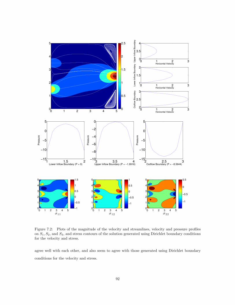
as Dirichlet boundary conditions for the velocity on S1, S2, and S3. Figure 7.2 depicts the magni-
tude of the velocity and streamlines, the horizontal velocity and pressure profile on each defective
boundary, and a contour plot of each stress component of the solution generated using the Dirichelt
boundary conditions.
7.6.1 Flow Rate Boundary Condition
The chosen Dirichlet boundary conditions yield flow rates of Q1 = − 43 , Q2 = − 2
3 , and
Q3 = 2 which were then used as flow rate boundary conditions for the flow matching problem.
Both algorithms used the constant vector g = [0.1, ..., 0.1] as an initial guess for both Dirichlet and
Neumann controls. On both meshes, the steepest descent algorithm converged in 13 iterations, and
the Gauss-Newton algorithm converged in three iterations. The results from the steepest descent
and Gauss-Newton algorithms displayed in Figures 7.3 and 7.4, respectively, as velocity streamlines,
inlet and outlet velocity and pressure profiles, and stress contours. The results from these algorithms
91
0 1 2 3 4 50
1
2
3
4
5
0
0.5
1
1.5
2
2.5
0 1 2 31
1.5
2
Horizontal Velocity
Low
er
Inflow
Boundary
0 1 2 33
3.5
4
Horizontal Velocity
Upper
Inflow
Boundary
0 1 2 32
2.5
3
Horizontal Velocity
Outflo
w B
oundary
1 1.5 2−15
−10
−5
0
5
Pre
ssu
re
Lower Inflow Boundary (P = 0)3 3.5 4
−10
−8
−6
−4
−2
0
Pre
ssu
re
Upper Inflow Boundary (P = −1.9916)2 2.5 3
−15
−10
−5
0
5
Pre
ssu
re
Outflow Boundary (P = −8.5644)
σ11
0 1 2 3 4 50
1
2
3
4
5
−1
−0.5
0
0.5
1
1.5
σ12
0 1 2 3 4 50
1
2
3
4
5
−1
−0.5
0
0.5
1
σ22
0 1 2 3 4 50
1
2
3
4
5
−1
−0.5
0
0.5
Figure 7.2: Plots of the magnitude of the velocity and streamlines, velocity and pressure profileson S1, S2, and S3, and stress contours of the solution generated using Dirichlet boundary conditionsfor the velocity and stress.
agree well with each other, and also seem to agree with those generated using Dirichlet boundary
conditions for the velocity and stress.
92
0 1 2 3 4 50
1
2
3
4
5
0
0.5
1
1.5
2
2.5
0 1 2 31
1.5
2
Horizontal Velocity
Low
er
Inflow
Boundary
0 1 2 33
3.5
4
Horizontal Velocity
Upper
Inflow
Boundary
0 1 2 32
2.5
3
Horizontal Velocity
Outflo
w B
oundary
1 1.5 2−5
0
5
10
Pre
ssure
Lower Inflow Boundary (P = 0)3 3.5 4
−4
−2
0
2
4
Pre
ssure
Upper Inflow Boundary (P = −1.9916)2 2.5 3
−10
−5
0
5
10
Pre
ssure
Outflow Boundary (P = −8.5644)
σ11
0 1 2 3 4 50
1
2
3
4
5
−0.5
0
0.5
1
1.5
σ12
0 1 2 3 4 50
1
2
3
4
5
−1
−0.5
0
0.5
1
σ22
0 1 2 3 4 50
1
2
3
4
5
−1.5
−1
−0.5
0
0.5
1
Figure 7.3: Plots of the magnitude of the velocity and streamlines, velocity and pressure profileson S1, S2, and S3, and stress contours of the solution generated using the steepest descent algorithmfor the flow rate matching problem with initial guess g = [0.1, ..., 0.1].
7.6.2 Mean Pressure Boundary Condition
Using the Dirichlet boundary conditions we computed the mean pressure on all of the defec-
tive boundaries, and then shifted the numerical solution so that the mean pressure on S1, P1, is zero.
93
0 1 2 3 4 50
1
2
3
4
5
0
0.5
1
1.5
2
2.5
0 1 2 31
1.5
2
Horizontal Velocity
Low
er
Inflow
Boundary
0 1 2 33
3.5
4
Horizontal Velocity
Upper
Inflow
Boundary
0 1 2 32
2.5
3
Horizontal Velocity
Outflo
w B
oundary
1 1.5 2−10
−5
0
5
10
Pre
ssu
re
Lower Inflow Boundary (P = 0)3 3.5 4
−4
−2
0
2
4
Pre
ssu
re
Upper Inflow Boundary (P = −1.9916)2 2.5 3
−10
−5
0
5
10
Pre
ssu
re
Outflow Boundary (P = −8.5644)
σ11
0 1 2 3 4 50
1
2
3
4
5
−0.5
0
0.5
1
1.5
σ12
0 1 2 3 4 50
1
2
3
4
5
−1
−0.5
0
0.5
1
σ22
0 1 2 3 4 50
1
2
3
4
5
−1
0
1
Figure 7.4: Plots of the magnitude of the velocity and streamlines, velocity and pressure profileson S1, S2, and S3, and stress contours of the solution generated using the Gauss-Newton algorithmfor the flow rate matching problem with initial guess g = [0.1, ..., 0.1].
Using this shifted solution the mean pressure on S2 and S3 (used for the mean pressure matching
problem) is P2 = −1.992 and P3 = −8.564. A solution (seen in Figure 7.5) was generated using the
steepest descent algorithm using Neumann and Dirichlet controls. The steepest descent algorithm
94
converged in four iterations on both meshes. We observe from Figure 7.5 that the velocity stream-
lines generally agree with those found using Dirichlet boundary conditions and flow rate matching,
but there are significant differences in the speed contours, inlet/outlet velocity and pressure profiles,
as well as in the σ12 stress component at the inlets and outlet.
7.6.3 Further flow rate boundary conditions algorithm verification
As further verification of our steepest descent and Gauss-Newton algorithms for flow rate
matching, we consider again both algorithms, but now with the constant vector g = [5, ..., 5] as
an initial guess for both controls. Both algorithms converged, with the steepest descent needing
17 iterations while the Gauss-Newton algorithm converged in three iterations. The solutions are
displayed in Figures 7.6-7.7, respectively, and we observe they match each other exactly, but are
quite different from the solutions found with initial guess g = [0.1, ..., 0.1]. These and previous
results indicate that both algorithms converge to a same local minimum and the local minimum
found by the algorithms is determined by an initial guess.
95
0 1 2 3 4 50
1
2
3
4
5
0
0.5
1
1.5
2
2.5
0 1 2 31
1.5
2
Horizontal Velocity
Low
er
Inflow
Boundary
0 1 2 33
3.5
4
Horizontal Velocity
Upper
Inflow
Boundary
0 1 2 32
2.5
3
Horizontal Velocity
Outflo
w B
oundary
1 1.5 2−15
−10
−5
0
5
Pre
ssu
re
Lower Inflow Boundary (P = 0)3 3.5 4
−8
−6
−4
−2
0
2
Pre
ssu
re
Upper Inflow Boundary (P = −1.9916)2 2.5 3
−15
−10
−5
0
5
10P
ressu
re
Outflow Boundary (P = −8.5644)
σ11
0 1 2 3 4 50
1
2
3
4
5
−0.5
0
0.5
1
σ12
0 1 2 3 4 50
1
2
3
4
5
−1
−0.5
0
0.5
1
σ22
0 1 2 3 4 50
1
2
3
4
5
−1
−0.5
0
0.5
1
1.5
Figure 7.5: Plots of the magnitude of the velocity and streamlines, velocity and pressure profileson S1, S2, and S3, and stress contours of the solution generated using the steepest descent algorithmfor the mean pressure matching problem with initial guess g = [0.1, ..., 0.1].
96
0 1 2 3 4 50
1
2
3
4
5
0
0.5
1
1.5
2
2.5
3
0 1 2 31
1.5
2
Horizontal Velocity
Low
er
Inflow
Boundary
0 1 2 33
3.5
4
Horizontal Velocity
Upper
Inflow
Boundary
0 1 2 32
2.5
3
Horizontal Velocity
Outflo
w B
oundary
1 1.5 2−10
0
10
20
Pre
ssu
re
Lower Inflow Boundary (P = 0)3 3.5 4
−10
−5
0
5
10
15
Pre
ssu
re
Upper Inflow Boundary (P = −1.9916)2 2.5 3
−10
0
10
20P
ressu
re
Outflow Boundary (P = −8.5644)
σ11
0 1 2 3 4 50
1
2
3
4
5
−1
0
1
2
3
4
σ12
0 1 2 3 4 50
1
2
3
4
5
−2
0
2
4
σ22
0 1 2 3 4 50
1
2
3
4
5
0
2
4
Figure 7.6: Plots of the magnitude of the velocity and streamlines, velocity and pressure profileson S1, S2, and S3, and stress contours of the solution generated using the steepest descent algorithmfor the flow rate matching problem with initial guess g = [5, ..., 5].
97
0 1 2 3 4 50
1
2
3
4
5
0
0.5
1
1.5
2
2.5
3
3.5
0 1 2 31
1.5
2
Horizontal Velocity
Low
er
Inflow
Boundary
0 1 2 33
3.5
4
Horizontal Velocity
Upper
Inflow
Boundary
0 1 2 32
2.5
3
Horizontal Velocity
Outflo
w B
oundary
1 1.5 2−10
0
10
20
Pre
ssu
re
Lower Inflow Boundary (P = 0)3 3.5 4
−10
0
10
20
Pre
ssu
re
Upper Inflow Boundary (P = −1.9916)2 2.5 3
−10
0
10
20P
ressu
re
Outflow Boundary (P = −8.5644)
σ11
0 1 2 3 4 50
1
2
3
4
5
0
2
4
6
σ12
0 1 2 3 4 50
1
2
3
4
5
−2
0
2
4
σ22
0 1 2 3 4 50
1
2
3
4
5
0
2
4
6
Figure 7.7: Plots of the magnitude of the velocity and streamlines, velocity and pressure profileson S1, S2, and S3, and stress contours of the solution generated using the Gauss-Newton algorithmfor the flow rate matching problem with initial guess g = [5, ..., 5].
98
Chapter 8
Conclusions
This work began in Chapter 3 where we studied a finite element method for the time-
dependent NSE based on the recently developed VVH formulation. Through a rigorous stability
analysis we have shown that the velocity is unconditionally stable, as is the vorticity if we penalize
the discrete solution to be ‘close’, in some sense, to the curl of the discrete velocity. Numerical
experiments show mixed results: for an idealized problem, optimal convergence rates are recovered
for the velocity and near-optimal convergence rates are recovered for the vorticity. However, on
channel flow problems over a step, it is clear that improved vorticity boundary conditions need to
be developed in order for this method to be competitive when higher order elements are used. In
Chapter 4 we addressed this problem by proposing a new, simple vorticity boundary condition. This
boundary condition, intended for portions of the domain where no-slip velocity boundary conditions
are to be enforced, was derived directly from the vorticity equation, and consisted of boundary
integrals of the pressure and forcing function. A 3d finite element method was then presented to
solve the steady NSE and vorticity equations implementing our new vorticity boundary conditions.
On a simple 3d problem, we verified that optimal convergence rates are achieved for the velocity
and vorticity solutions, and we are currently working on performing several 3d benchmark problems
to further test the method.
Chapter 5 derived a new, reduced order MDM, based off of the original MDM proposed
in [22]. The RMDM allowed us to derive a C0 finite element method that is unconditionally sta-
ble. Additionally, the method consists of a linearized backward Euler timestepping scheme which
decouples the filter solve, making the method efficient. We then proved analytically that optimal
99
convergence rates are achieved (with respect to the model solution). The chapter ended by imple-
menting our method on two benchmark 2d flow problems. In both examples, more accurate solutions
are recovered from the RMDM when we use two different spatial scales for the filters, verifying the
effectiveness of our multiscale model.
Our study of the defective boundary problem for non-Newtonian flows began in Chapter
6, where we considered a numerical method for generalized-Newtonian flows governed by the Cross
model with flow rate boundary conditions. The problem was formulated as a constrained optimal
control problem for which we proved solutions must exist. We then proved the existence of Lagrange
multipliers, and used the Lagrange multiplier method to derive an optimality system. Finally, a
steepest descent method was proposed that decouples the optimality system. We ended the chapter
by studying a complex 2d flow problem for which we were able to accurately and efficiently produce
solutions, verifying the robustness of our numerical method.
Chapter 7 investigated two numerical methods for viscoelastic flows with flow rate or mean
pressure boundary conditions. As in Chapter 6, the defective boundary problem was transformed
into an optimal control problem. The first method to solve this system stems from that presented
in Chapter 6, where an optimality system is derived using the Lagrange multiplier method, and a
steepest descent method is used to decouple and solve the optimality system. The second method
reconsidered the optimality system from a nonlinear least squares (NLS) viewpoint. We solved the
NLS problem by solving a related linear least squares problem (which was done using a conjugate
gradient method). Finally, a numerical experiment was considered to compare and contrast the two
methods, showing that the former is more robust, but the latter is more efficient.
1186 // // Output p o i n t s ( v o r t i c i t y )
1187 // doub le n=50;
1188 // s t d : : vec tor<double> xvec (n) ;
1189 // s t d : : vec tor<double> yvec (n) ;
1190 // s t d : : vec tor<double> zvec (n) ;
1191
1192 // f o r ( doub le i x =0; ix<n ; i x++)
1193 //
1194 // xvec [ i x ] = i x /(n−1) ;
1195 // yvec [ i x ] = i x /(n−1) ;
1196 // zvec [ i x ] = i x /(n−1) ;
1197 //
1198
1199 // doub le w1val , w2val , w3val ;
1200 // Vector<double> s o l u t i o n v a l ( dim ) ;
1201
1202 // s t d : : s t r i n g f i l ename = outpath+”V o r t i c i t y V a l u e s ” ;
147
1203 // s t d : : o fs tream output ( f i l ename . c s t r ( ) ) ;
1204 // output << xvec . s i z e ( ) << ” ” << yvec . s i z e ( ) << ” ” << zvec . s i z e ( )
<< ” ” << xvec . s i z e ( ) << ” ” << yvec . s i z e ( ) << ” ” << zvec . s i z e ( )
<< ” ” << s t d : : end l ;
1205
1206 // f o r ( unsigned i n t i x = 0; i x < xvec . s i z e ( ) ; i x++)
1207 //
1208 // s t d : : cout << ” i x = ” << i x << s t d : : end l ;
1209
1210 // f o r ( unsigned i n t i y = 0; i y < yvec . s i z e ( ) ; i y++)
1211 // f o r ( unsigned i n t i z = 0; i z < zvec . s i z e ( ) ; i z++)
1212 //
1213 // VectorTools : : p o i n t v a l u e ( d o f h a n d l e r v o r t , s y s t e m r h s v o r t
, Point<dim> ( xvec [ i x ] , yvec [ i y ] , zvec [ i z ] ) , s o l u t i o n v a l ) ;
1214
1215 // w1val = s o l u t i o n v a l [ 0 ] ;
1216 // w2val = s o l u t i o n v a l [ 1 ] ;
1217 // w3val = s o l u t i o n v a l [ 2 ] ;
1218
1219 // output << xvec [ i x ] << ” ” << yvec [ i y ] << ” ” << zvec [ i z ]
<< ” ” << w1val << ” ” << w2val << ” ” << w3val << ” ” << s t d : :
end l ;
1220 //
1221 //
1222 //
1223
1224
1225
1226 /∗∗∗∗∗∗∗∗ ∗/
1227 /∗ Run ∗/
148
1228 /∗∗∗∗∗∗∗∗ ∗/
1229
1230 template <int dim>
1231 void SNSE<dim> : : run ( )
1232
1233 Timer ProgramTimer ;
1234 ProgramTimer . s t a r t ( ) ;
1235
1236 make grid ( ) ;
1237 setup system ( ) ;
1238
1239 double NLerr = 1 ;
1240 int NLiter = 0 ;
1241
1242 while ( ( NLerr>1e−6) && ( NLiter < 10) )
1243
1244 std : : cout << std : : endl << ”∗∗∗ Newton i t e r a t i o n ” << NLiter+1 << ”
∗∗∗” << std : : endl ;
1245 p r e v s o l u t i o n v e l = s y s t e m r h s v e l ;
1246
1247 a s s em b l e v e l o c i t y s y s t e m ( ) ;
1248 s o l v e v e l ( ) ;
1249
1250 i f ( NLiter > 0)
1251 NLerr = compute re lat ive norm ( ) ;
1252
1253 NLiter++;
1254
1255
1256 i f ( NLerr < 1e−6)
149
1257 std : : cout << std : : endl << ”∗∗∗ Newton method converged in ” <<
NLiter << ” i t e r a t i o n s ∗∗∗” << std : : endl ;
1258
1259 a s s e m b l e v o r t i c i t y s y s t e m ( ) ;
1260 s o l v e v o r t ( ) ;
1261
1262 compute error ( ) ;
1263 // o u t p u t r e s u l t s ( ) ;
1264
1265 ProgramTimer . stop ( ) ;
1266 std : : cout << std : : endl << ” Total wa l l time : ” << std : : f l o o r (
ProgramTimer . wa l l t ime ( ) + 0 . 5 ) << ” seconds ” << std : : endl ;
1267
1268
1269
1270 /∗ ∗∗∗∗∗∗∗∗∗∗∗∗∗∗∗∗ ∗/
1271 /∗ Main Function ∗/
1272 /∗ ∗∗∗∗∗∗∗∗∗∗∗∗∗∗∗∗ ∗/
1273 int main ( )
1274
1275 using namespace d e a l i i ;
1276 d e a l l o g . depth conso l e (0 ) ;
1277
1278 SNSE<3> f low problem 3d ;
1279 f low problem 3d . run ( ) ;
1280
1281
1282 return 0 ;
1283
150
Bibliography
[1] F. Abrahan, M. Behr, and M. Heinkenschloss. Shape optimization in unsteady blood flow: Anumerical study of non-newtonain effects. Comput. Methods Biomech. Biomed. Engng., 8:201–212, 2005.
[2] N. A. Adams and S. Stolz. On the Approximate Deconvolution procedure for LES. Phys. Fluids,2:1699–1701, 1999.
[3] N. A. Adams and S. Stolz. Deconvolution methods for subgrid-scale approximation in largeeddy simulation. Modern Simulation Strategies for Turbulent Flow, 2001.
[4] J. C. Andre and M. Lesieur. Influence of helicity on high Reynolds number isotropic turbulence.Journal of Fluid Mechanics, 81:187–207, 1977.
[5] B.F. Armaly, F. Durst, J.C.F. Pereira, and B. Schonung. Experimental and theoretical inves-tigation of backward-facing step flow. Journal of Fluid Mechanics, 127:473–496, 1983.
[6] W. Bangerth, R. Hartmann, and G. Kanschat. deal.II – a general purpose object oriented finiteelement library. ACM Trans. Math. Softw., 33(4):24/1–24/27, 2007.
[7] W. Bangerth, T. Heister, G. Kanschat, et al. deal.II Differential Equations Analysis Library,Technical Reference. http://www.dealii.org.
[8] J. Baranger and K. Najib. Analyse numerique des ecoulements quasi-Newtoniens dont la vis-cosite obeit a la loi puissance ou la loi de carreau. Numerical Mathematics, 58:35–49, 1990.
[9] L.C. Berselli and D. Cordoba. On the regularity of the solutions to the 3d Navier-Stokesequations: a remark on the role of the helicity. Comptes Rendus Mathematique, 347(11-12):613–618, 2009.
[10] F. Brezzi and M. Fortin. Mixed and Hybrid Finite Element Methods, volume 15 of SpringerSeries in Computational Mathematics. Springer-Verlag, 1991.
[11] J. Burkardt and M. Gunzburger. Sensitivity discrepancy for geometric parameters. CFD forDesign and Optimization, ASME, New York, pages 9–15, 1995.
[12] Q. Chen, S. Chen, and G. Eyink. The joint cascade of energy and helicity in three dimensionalturbulence. Physics of Fluids, 15(2):361–374, 2003.
[13] Q. Chen, S. Chen, G. Eyink, and D. Holm. Intermittency in the joint cascade of energy andhelicity. Physical Review Letters, 90: 214503, 2003.
[14] S.-S. Chow and G. F. Carey. Numerical approximation of generalized Newtonian fluids usingPowell-Sabin-Heindl elements: I. theoretical estimates. International Journal for NumericalMethods in Fluids, 41(10):1085–1118, 2003.
151
[15] B. Cousins, L. Rebholz, and N. Wilson. Enforcing energy, helicity and strong mass conservationin FE computations for incompressible Navier-Stokes simulations. Applied Mathematics andComputation, 281:1208–1221, 2011.
[16] M. Cross. Rheology of non-Newtonian fluids: A new flow equation for pseudo plastic systems.Journal of Colloid Science, 20(5):417–437, 1965.
[17] C. Davies and P. W. Carpenter. A novel velocity-vorticity formulation of the Navier-Stokesequations with applications to boundary layer disturbance evolution. Journal of ComputationalPhysics, 172:119–165, 2001.
[18] S. De, K. Nagendra, and K.N. Lakshmisha. Simulation of laminar flow in a three-dimensionallid-driven cavity by the Lattice-Boltzmann method. International Journal of Numerical Methodsfor Heat and Fluid Flow, 19(6):790–815, 2009.
[19] P. Ditlevsen and P. Giuliani. Dissipation in helical turbulence. Physics of Fluids, 13, 2001.
[20] P. Ditlevson and P. Guiliani. Cascades in helical turbulence. Physical Review E, 63, 2001.
[21] Q. Du, M. Gunzburger, and L.S. Hou. Analysis and finite element approximation of opti-mal control problems for a Ladyzhenskaya model for stationary, incompressible viscous flows.Journal of Computational and Applied Mathematics, 61:323–343, 1995.
[22] A. Dunca. A two-level multiscale deconvolution method for the large eddy simulation of tur-bulent flows. Mathematical Models and Methods in Applied Sciences, 22(6):1–30, 2012.
[23] V.J. Ervin and N. Heuer. Approximation of time-dependent, viscoelastic fluid flow: Crank-Nicolson, finite element approximation. Numer. Methods Partial Differential Eq., 20:248–283,2003.
[24] V.J. Ervin and H.K. Lee. Numerical approximation of a quasi-newtonian stokes flow problemwith defective boundary conditions. SIAM J. Numer. Anal., 45:2120–2140, 2007.
[25] C. Foias, L. Hoang, and B. Nicolaenko. On the helicity in 3D-periodic Navier-Stokes equationsI: The non-statistical case. Proc. London Math. Soc., 94:53–90, 2007.
[26] L. Formaggia, J. F. Gerbeau, F. Nobile, and A. Quarteroni. Numerical treatment of defectiveboundary conditions for the Navier-Stokes equations. SIAM J. Numer. Anal., 40:376–401, 2002.
[27] L. Formaggia, A. Veneziani, and C. Vergara. A new approach to numerical solution of defectiveboundary value problems in incompressible fluid dynamics. SIAM J. Numer. Anal., 46:2769–2794, 2008.
[28] G.P. Galdi. An introduction to the Mathematical Theory of the Navier-Stokes Equations, VolumeI. Springer, Berlin, 1994.
[29] K. Galvin, H.K. Lee, and L. Rebholz. Approximation of viscoelastic flows with defective bound-ary conditions. Journal of Non-Newtonian Fluid Mechanics, 169-170:104–113, 2012.
[30] V. Girault and P.-A. Raviart. Finite element methods for Navier-Stokes equations : Theoryand algorithms. Springer-Verlag, 1986.
[31] G. Golub and C. Van Loan. Matrix Computations. Johns Hopkins University, Baltimore, 1989.
[32] P. Gresho and R. Sani. Incompressible Flow and the Finite Element Method, volume 2. Wiley,1998.
[33] C.W. Groetsch. Generalized Inverses of Linear Operators. Marcel Dekker, New York, 1977.
152
[34] S. Großand and A. Reusken. Numerical Methods for Two-phase Incompressible Flows. Springer,Berlin, 2011.
[35] M. Gunzburger. Perspectives on Flow Control and Optimization. SIAM, 2003.
[36] M. Gunzburger, L. Hou, and T. Svobodny. Heating and cooling control of temperature distri-butions along boundaries of flow domains. J. Math. Syst. Estimat. Control, 3:147–172, 1993.
[37] M. Gunzburger and H.-C. Lee. Analysis, approximation, and computation of a coupledsolid/fluid temperature control problem. Comput. Methods Appl. Mech. Engrg., 118(1-2):133–152, 1994.
[38] M. Gunzburger and H. Wood. Adjoint and sensitivity-based methods for optimization of gascentrifuges. in:Proceedings of 7th Work. Separation Phenomena in Liquids and Gases; MoscowEngineering Physics Institute, 2000.
[39] F. Hecht, O. Pironneau, and K. Ohtsuka. Software freefem++. http://www.freefem.org, 2005.
[40] J. Heywood and R. Rannacher. Finite element approximation of the nonstationary Navier-Stokes problem. Part IV: Error analysis for the second order time discretization. SIAM J.Numer. Anal., 2:353–384, 1990.
[41] J. G. Heywood, R. Rannacher, and S. Turek. Artificial boundaries and flux and pressureconditions for the incompressible Navier-Stokes equations. Int. J. Numer. Methods Fluids,22:325–352, 1996.
[42] M. Hribersek, L. Skerget, and Z. Zunic. 3d driven cavity flow by mixed boundary and finiteelement method. In European Conference on Computational Fluid Dynamics, ECCOMAS CFD,2006.
[43] V. John and A. Liakos. Time dependent flow across a step: the slip with friction boundarycondition. International Journal of Numerical Methods in Fluids, 50:713 – 731, 2006.
[44] J. Kim, H. Le, and P. Moin. Direct numerical simulation of turbulent flow over a backward-facing step. Journal of Fluid Mechanics, 330:349–374, 1997.
[45] K. Kunisch and X. Marduel. Optimal control of non-isothermal viscoelastic fluid flow. Journalof Non-Newtonian Fluid Mechanics, 80:261–301, 2000.
[46] W. Layton. An introduction to the numerical analysis of viscous incompressible flows. SIAM,2008.
[47] W. Layton and L. Rebholz. Approximate Deconvolution Models of Turbulence: Analysis, Phe-nomenology and Numerical Analysis. Springer, 2012.
[48] H.K. Lee. Optimal control for quasi-Newtonian flows with defective boundary conditions. Com-put. Methods. Appl. Mech. Engrg., 200:2498–2506, 2011.
[49] H.K. Lee and H.C. Lee. Analysis and finite element approximation of an optimal control problemfor the oseen viscoelastic fluid flow. J. Math. Anal. Appl., 336:1090–1160, 2007.
[50] H.K. Lee, M.A. Olshanskii, and L.G. Rebholz. On error analysis for the 3D Navier-Stokesequations in Velocity-Vorticity-Helicity form. SIAM Journal on Numerical Analysis, 49(2):711–732, 2011.
[51] C. Manica, M. Neda, M.A. Olshanskii, L. Rebholz, and N. Wilson. On an efficient finite elementmethod for Navier-Stokes-omega with strong mass conservation. Computational Methods inApplied Mathematics, 11(1):3–22, 2011.
153
[52] H. L. Meitz and H. F. Fasel. A compact-difference scheme for the Navier-Stokes equations invorticity-velocity formulation. Journal of Computational Physics, 157:371–403, 2000.
[53] H. Moffatt and A. Tsoniber. Helicity in laminar and turbulent flow. Annual Review of FluidMechanics, 24:281–312, 1992.
[54] M.A. Olshanskii. A fluid solver based on vorticity-helical density equations with application toa natural convection in a cubic cavity. Int. J. Num. Meth. Fluids, 2011.
[55] M.A. Olshanskii and L. Rebholz. Velocity-Vorticity-Helicity formulation and a solver for theNavier-Stokes equations. Journal of Computational Physics, 229:4291–4303, 2010.
[56] M.A. Olshanskii and L. Rebholz. Application of barycenter refined meshes in linear elasticityand incompressible fluid mechanics. ETNA: Electronic Transactions in Numerical Analysis,38:258–274, 2011.
[57] J. Qin. On the convergence of some low order mixed finite elements for incompressible fluids.PhD thesis, Pennsylvania State University, 1994.
[58] L. Rebholz. Efficient, unconditionally stable, and optimally accurate FE algorithms for approx-imate deconvolution models of fluid flow, submitted.
[59] V. Ruas. A new formulation of the three-dimensional velocity-vorticity system in viscous in-compressible flow. Math. Mech., 79:29–36, 1999.
[60] L.R. Scott and M. Vogelius. Conforming finite element methods for incompressible and nearlyincompressible continua. volume Lectures in Applied Mathematics, 22-2 of Large-scale compu-tations in fluid mechanics, Part 2, pages 221–244. Amer. Math. Soc., 1985.
[61] J. Trujillo and G. E. Karniadakis. A penalty method for the vorticity-velocity formulation.Journal of Computational Physics, 149:32–58, 1999.
[62] K.L. Wong and A.J. Baker. A 3d incompressible Navier-Stokes velocity-vorticity weak formfinite element algorithm. International Journal for Numerical Methods in Fluids, 38:99–123,2002.
[63] X.H. Wu, J.Z. Wu, and J.M. Wu. Effective vorticity-velocity formulations for the three dimen-sional incompressible viscous flows. Journal of Computational Physics, 122:68–82, 1995.
[64] E. Zeidler. Nonlinear Functional Analysis and its Applications, volume III. Springer, NewYork, 1985.
[65] S. Zhang. A new family of stable mixed finite elements for the 3d Stokes equations. Mathematicsof Computation, 74:543–554, 2005.
[66] S. Zhang. Divergence-free finite elements on tetrahedral grids for k ≥ 6. Math. Comp., 80:669–695, 2011.
[67] S. Zhang. Quadratic divergence-free finite elements on Powell-Sabin tetrahedral grids. Calcolo,48:211–244, 2011.