Algae Biomonitoring and Assessment for Streams and Rivers of

Algae Biomonitoring and Assessment for

Streams and Rivers of California's Central

Coast

Scott L. Rollins, Ph.D.

Spokane Falls Community College

Spokane, WA 99224-5288

Marc Los Huertos, Ph.D.

California State University, Monterey Bay

Seaside, CA 93955-8001

Pam Krone-Davis

California State University, Monterey Bay

Seaside, CA 93955-8001

Charles (Cory) Ritz, M.S.

Ulster County Soil and Water Conservation District

Phoenicia, NY 12464

Table of Contents

Introduction ................................................................................................................................ 1

Background ................................................................................................................................. 3

Bioassessment ....................................................................................................................... 3

Defining “Reference Condition” for this Document ................................................. 5

Application of Reference Sites to Establish Expected Conditions ....................... 6

Algal Ecology .......................................................................................................................... 6

Diatom Characteristics ................................................................................................................. 7

Diatoms and Nutrients ................................................................................................................. 7

Nutrient Enrichment on California’s Central Coast ......................................................... 8

Applying the IBI for Development of Effects-based Criteria ................................. 9

RIVPACS ................................................................................................................................ 10

Overview of RIVPACS ................................................................................................................ 10

Implication of a RIVPACS application in Coastal California ....................................... 12

Report Organization ......................................................................................................... 13

METHODS .................................................................................................................................. 13

Sampling Design and Sample Collection ................................................................... 14

Field and Laboratory Water Chemistry Methods ................................................... 15

Quality Assurance ....................................................................................................................... 17

Geographic Information System Methods ................................................................ 17

Reference/Nonreference Site Determination ......................................................... 18

Quantifying the Human Disturbance Gradient ....................................................... 19

Index of Biological Integrity .......................................................................................... 19

ALGAE BIOASSESSMENT FOR CALIFORNIA’S CENTRAL COAST ii

Algae Metric Screening and Selection ................................................................................. 19

Metric Classification ................................................................................................................... 20

Individual Metric Range ........................................................................................................... 21

Reproducibility ............................................................................................................................. 21

Responsiveness ............................................................................................................................ 22

Accounting for Natural Gradients......................................................................................... 22

Scaling, Direction-Corrections, and IBI Calculation ...................................................... 22

Using the IBI to Establish Biocriteria ......................................................................... 23

RIVPACS ................................................................................................................................ 25

Site Classification Based on Diatom Assemblages ......................................................... 25

Predictor Variables ..................................................................................................................... 25

Predictive Model .......................................................................................................................... 26

Results and Discussion ......................................................................................................... 29

Taxonomical Results ........................................................................................................ 29

Metric Screening ................................................................................................................ 30

Diatom Index of Biotic Integrity (IBI) for wadable streams and rivers of

California's Central Coast ............................................................................................... 31

Identifying Potential IBI-based Water Quality Criteria ............................................... 35

Application of the IBI to Recommend Effects-based Criteria ............................ 36

RIVPACS ................................................................................................................................ 37

Conclusions ............................................................................................................................... 38

References ................................................................................................................................ 97

Appendix I: Calculating the IBI for New Samples ...................................................... 106

Appendix II: Calculating O/E for New Samples .......................................................... 107

ALGAE BIOASSESSMENT FOR CALIFORNIA’S CENTRAL COAST iii

List of Tables & Figures

Tables Table 1. Environmental Factors that affect diatom growth .................................................................. 7 Table 2. Methods used for chemical analysis of water samples ........................................................ 15 Table 3. DFG criteria for determination of reference site conditions ............................................. 39 Table 4. Site location and determination of site type ..................................................................... 40- 45 Table 5 Candidate metric classifications ............................................................................................. 46-55 Table 6. Suggested boundaries for stream trophic classifications ................................................... 24 Table 7. Candidate variables used to predict site assemblage classes ........................................... 56 Table 8. The number of sites where diatom species were found ................................................ 57-66 Table 9. The number of sites where soft algae species were found ................................................. 67 Table 10. IBI Metrics for California’s Central Coast ............................................................................... 68

Figures Figure 1. Example of diatoms from California Central Coast………………………………………….….…..7

Figure 2. Process overview of RIVPACS method………………………………………………………………….11

Figure 3. Central Coast region and sample sites ..................................................................................... 69 Figure 4. Reference sites ................................................................................................................................. 70 Figure 5. Nonreference sites .......................................................................................................................... 71 Figure 6. Histograms of log abundance for the most prevalent species……………………..……72-74Figure 7. Boxplots of individual MAIBI metrics to human disturbance. ................................. 75-80 Figure 8. Response (MAIBI) to the human disturbance gradient ..................................................... 81 Figure 9. Boxplots relating IBI to human disturbance. ........................................................................ 82 Figure 10. Boxplots of IBI for reference and nonreference sites ..................................................... 83 Figure 11. IBI thresholds for eutrophic and trophic status indices ................................................ 84 Figure 12. Threshold for the MAIBI using the PCA-derived trophic status index as the

endpoint ............................................................................................................................................................ 85 Figure 13. Change-point analysis of stressor-response variables TN and TP. ............................. 86 Figure 14. Nonparametric changepoint analysis for TN-Suspended and Benthic Chlorophyll

stressor-response relationships ............................................................................................................... 87 Figure 15. Nonparametric changepoint analysis applied to the TP-Suspended and Benthic

Chlorophyll stressor-response relationships ...................................................................................... 88 Figure 16. Nonparametric changepoint analysis applied to the nitrate-MIABI relationship . 89 Figure 17. Histograms of nitrogenous compounds for Reference and Nonreference .............. 90 Figure 18. Site assemblage dendogram ...................................................................................................... 91 Figure 19. Observed versus Expected Species Richness ...................................................................... 92 Figure 20. Boxplots of RIVPACS Calibration, Validation and Test Sites .......................................... 93 Figure 21. Distribution of O/E values for the calibration set………………………………………….……94

Figure 22. Proportion of metamorphic rock for watersheds . ........................................................... 95 Figure 23. Metamorphic rock on the Big Sur Coast ................................................................................ 96 Figure 24. Phosphorus samples associated with watersheds. ........................................................... 97

ALGAE BIOASSESSMENT FOR CALIFORNIA’S CENTRAL COAST 1

Introduction California has made substantial progress in the field of bioassessment over the past

20 years, since the California Department of Fish and Game published its first

standardized procedure on bioassessment in 1993. Both the California Water

Resources Control Board and the Department of Fish and Game have invested

considerable effort and resources in the development of programs, research and

expertise in the field. These efforts have been made in recognition of the economic

importance of preserving the health and integrity of California's aquatic ecosystems

for beneficial uses, as well as to meet the requirements of the Clean Water Act to

"restore and maintain the chemical, physical and biological integrity of the nations

waters." The California Department of Fish and Game (CDFG) has an Aquatic

Bioassessment Laboratory dedicated to the mission of "supporting the use of

biology in California's water quality management and assessment programs." The

CA Department of Pesticide Regulation has used bioassessment as a tool for

ascertaining reference conditions and documenting expected macro-invertebrate

communities in specific areas of interest for pesticide effects, for example the San

Joaquin Valley (Bacey 2007). The progress that has been made in California includes

the consolidation of data management from multiple programs under the Surface

Water Ambient Management Program (SWAMP), development of citizen monitoring

programs, field methods courses, extensive guidance for quality assurance,

protocols and tools, and investment by several of California’s regions in the

development of indices of biological integrity (IBI). In 2009, an external review of

California's bioassessment program concluded that while the state had made great

strides forward in the field of bioassessment, technical recommendations for further

advancement included the addition of algal assemblages for bioassessment and the

implementation of the Reference Condition Management Plan, which was published

in 2009 (Yoder and Plotnicoff 2009).

Bioassessment is one of several biological monitoring tools, which include toxicity

monitoring, tissue chemistry, invasive and indicator species monitoring and the

development of fish habitat indices. The purpose of bioassessment is to directly

characterize stream health through biological, rather than chemical of physical,

indicators. Methodologies for of bioassessment rely on the identification of

organism assemblages that occur in undisturbed or minimally disturbed sites and

expected under natural environmental conditions. One ways to quantify the

composition of these assemblages is through indices of biological integrity (IBI).

Macroinvertebrates had been California's primary biological indicator and were the

focus of the first regional IBIs (Herbst 2001). Multimetric indices of biological


integrity for BMI are available for the Eastern Sierras, the Northern Coast, the

Central Valley and the South Coast (SWAMP 2006). Tools have been developed and

published online for regional use for both the Eastern Sierras and the South &

Central Coast based on these IBIs for macroinvertebrates. These tools enable users

to characterization of the biological health of streams of interest based on regional

research of reference sites and the development of IBIs. In addition to IBIs,

predictive models of expected BMI assemblages based on natural environmental

gradients have been developed. Models, such as River Invertebrate Prediction and

Classification system (RIVPACS), use an observed to expected ratio to assess stream

health. Application of RIVPACS to macroinvertebrate populations have been used in

California streams (Hawkins et al. 2000, Ode et al. 2008), however evidence of

regional application of such models was not found during our literature review.

More recently Ecologstis and resource agencies have acknowledged the potential to

use freshwater algae assemblages for stream and river bioassessment.

Algae production, primarily in the form of suspended chlorophyll concentration, is

the most common way in which algae is applied in bioassessment in California. More

limited progress has been made in California in the use of algae species composition

for ecological characterization of stream health. Identification of periphyton

communities for bioassessement in California began in the Lahontan region in 1996.

In 2003, the Lahontan Region published a report identifying diatom and soft algae

species that could serve as indicators of environmental conditions and ecosystem

integrity for the Lahontan Basin (Blinn and Herbst 2003). Following their initial

study, they developed a preliminary index of biotic integrity (IBI) for the Eastern

Sierra Nevada region of California (Herbst and Blinn 2008). In 2007, Proposition 50

grants for the research funding this report on algae bioassessment and monitoring

in the Central Coast region of California and for Southern California were signed. In

2008 a technical advisory committee (TAC) composed of researchers, scientists and

regulators recommended that the California Water Resources Control Board include

algae as a bioassessment tool in SWAMP, focusing first on wadeable perennial

streams and later on nonperennial streams ( Fetscher and McLaughlin 2008). The

TAC encouraged use of diatoms and soft algae based on their responsiveness to

nutrients as a stressor, because they are helpful to diagnosing other forms of

impairment such as siltation or heavy metals, and as a way of meeting the USEPA

recommendation to use multiple indicators as lines of evidence, i.e. used in

conjunction with macroinvertebrate bioassessment. A further recommendation of

this team was to form a workgroup for taxonomic harmonization for stream algae in

the southwest. The Central Coast research team and the Southern California

research teams working on the Proposition 50 grants have worked collaboratively


to achieve harmonization of taxonomic identification. In 2011, a meeting between

the three labs involved in taxonomic identification (Portland State University,

University of Colorado, and Michigan State University) and project researchers

generated a harmonized taxonomy list, which included a master list with valid

names and images.

Our bioassessment of periphyton on California's Central Coast has been guided by a

technical advisory committee (TAC) including membership from the Southern

California Coastal Water Research Project (SCCWRP), the Central Coast Regional

Water Quality Control Board, the US Environmental Protection Agency, the US Fish

and Wildlife Service, the US Geological Survey, California State Parks and the

California Department of Fish and Game.

The goals of this study were multifold:

to expand the number of reference sites in the Central Coast Region and

characterize algae at these reference sites

to develop an algae index of biotic integrity (IBI) to help evaluate and

monitor water quality use in the Central Coast region

to develop a tool for use in classification of stream ecological condition

based on our IBI

to harmonize the taxa for the Central Coast and Southern Coast

quantify nutrient-algae relationships that will assist in the development of

nutrient criteria protective of beneficial uses.

to develop a predictive model, similar to River Invertebrate Prediction and

Classification system (RIVPACS), for determining an observed to expected

(O/E) ratio for diatom assemblages for potential use in characterizing

stream health on the Central Coast.

Background

Bioassessment

The Clean Water Act was written with the objective “to restore and maintain the

chemical, physical, and biological integrity of the Nation’s waters.” As a result of the

law, States and Tribes have monitored many chemical pollutants for decades and

evaluated biological integrity using laboratory toxicology assays. Researchers have

made considerable progress and developed sophisticated techniques for identifying

the chemical constituents of water quality and the potential sources of pollution


(Cude 2001); however, traditional monitoring of chemical water quality and

toxicological data can underestimate biological degradation by failing to assess the

extent of ecological damage in streams (USEPA 1996; Yagow et al. 2006).

Compounding the challenge to define ‘clean’ water is the complex and dynamic

nature of lotic systems and the range of characteristics such as biological, physical,

and chemical attributes of stream environments (Vannote et al. 1980; Resh et al.

1988; Dodds et al. 1998; Allan and Castillo 2007). Sole reliance on stream chemistry

monitoring is an incomplete indication of stream health; whereas, biological

indicators provide a more effective tool to monitor the ecological response to

physical and chemical stressors in the environment (Barbour et al. 1999; Karr 1999;

Karr and Chu 2000; Yagow et al. 2006).

Water quality, measured as the concentration of toxic chemicals and reduced

toxicity in bioassays, has generally improved through regulation of point-source

reductions. Over time, biological monitoring—primarily of fish and aquatic

invertebrates—has been incorporated by many States and Tribes and now

supplements laboratory toxicology assays (Karr 2006).

These monitoring approaches have shown some effectiveness in reducing point-

source pollutants; however, non-point source pollutants have been more difficult to

regulate and manage (Smith et al. 1999). Agriculturally derived nutrients are often

non-point source pollutants, entering waterways from diffuse locations rather than

discharge pipes. Biological monitoring can be complicated, as many biological

organisms respond indirectly rather than directly to nutrients, especially as their

impact cascades up the food web. Perhaps even more problematic to interpreting

the consequences of anthropogenically added nutrients, nitrogen and phosphorus,

unlike DDT or atrazine, are naturally found in aquatic ecosystems, are necessary to

the survival of living organisms, and can vary with non-anthropogenic factors such

as geology and climate. Thus, in cases where nutrient enrichment may threaten the

integrity of surface waters, accounting for background variation in nutrients and the

effect of increases on organisms that respond directly to nutrients in biological

monitoring and assessment may be important (Rollins 2005, Soranno et al. 2008).

Biological assessments and the associated biocriteria evaluate the integrity of

freshwater streams. Stream taxa, such as fish, invertebrates or diatoms, have the

potential to assimilate the effects from anthropogenic changes into their community

structure (Karr 1981; Wright et al. 1984; Barbour et al. 1999; Stevenson and Pan

1999). Changes in assemblage composition thus can be used to quantify changes in

the biological integrity of streams caused by changes in stream chemistry, physical


modifications, or introduction of non-indigenous species (Barbour et al. 1999;

Bailey et al. 2004). Biological integrity, in this instance, refers to the unimpaired

condition and the ability of aquatic taxa, communities and guilds to respond and

recover from natural fluctuations (Angermeier and Karr 1994; Karr 1999). As part

of the long-term national goals for clean water, the United States Congress

incorporated a concept of biological integrity into United States water quality policy.

The Federal Water Pollution Control Act Amendments of 1972 and 1987, referred to

as the Clean Water Act (CWA), requires federal and state governments to restore

and maintain the “biological integrity of the Nation’s waters” (USEPA 2002). The

CWA established the need to preserve and protect the biological integrity of aquatic

resources and institute the appropriate biocriteria to assess water quality.

Aquatic bioassessments interpret the ecological condition of a waterbody by

directly measuring the resident, surface-water biota (USEPA 1996). Bioassessments

often utilize communities of organisms to communicate broad meaning beyond the

measurement of a single organism (Karr 1981; Norris and Hawkins 2000). The

inferences of indicator species can aid scientific knowledge, policy and management

decisions and communicate the condition of a waterbody to a larger audience

(Norris and Hawkins 2000). Biocriteria can provide the narrative guidelines or the

numeric targets used to evaluate the biological integrity of a waterbody (USEPA

2000). States commonly designate the beneficial uses for a waterbody, such as

important fisheries or critical habitats for species of concern. Biocriteria help

evaluate and protect these aquatic life uses (USEPA 2000).

Defining “Reference Condition” for this Document

To evaluate the health of a system, researchers often compare sampled sites against

an expected condition. Expected conditions are often established through the use of

comparison sites that lack disturbances that are expected to affect water quality.

Historically, these were sites upstream of a point source of concern. This approach

is more problematic for water quality assessment when nutrient enrichment is a

suspected source of impairment. First, point sources of nutrients are less common

than non-point sources, making it difficult to identify a suitable upstream site.

Second, statistical inference based on upstream sites can be confounded due to lack

of sample independence. More recently, large field surveys that sample many sites

with minimal human disturbance throughout a region are being used to help

establish expected conditions at sites where impairment is suspected (Wang et al.

2005, Stevenson et al. 2008). These approaches that incorporate minimally

disturbed regional sites either apply a set of reasonably independent samples (i.e.,

spaced sufficiently to reduce the effects of spatial autocorrelation) within a physical


region of similar sites (e.g., the bioregion approach) or are used in combination with

abiotic factors such as climate, geology, and geography to model expected

conditions at individual sites (e.g., the RIVPACS approach).

Commonly, these minimally disturbed sites are referred to as “reference sites,”

despite potential for confusion in the use of this term. Stoddard et al. (2006) suggest

that the term “reference condition” should be reserved for sites that exemplify true

naturalness. However, in practice, the term “reference site” is applied to sites

establishing varying degrees of expected conditions. For example, in highly

disturbed regions, the expectation may be that reference sites reach “best attainable

conditions,” because these sites likely represent the best attainable conditions for

the region. In this study, we use the term “reference” to describe sites that range

from what Stoddard et al. call “minimally disturbed” to “least disturbed” allowing for

limited anthropogenic activities within the watershed.

Application of Reference Sites to Establish Expected Conditions

The reference condition approach (RCA) quantifies ecological conditions at sites

with minimal human disturbance and applies these values as the expected

conditions at test sites where water quality is being assessed. Bioassessments using

a RCA can measure the deleterious effects anthropogenic stressors have on

organisms by first measuring stream integrity at sites unaffected by human

influence. In other words, RCA establishes benchmarks with which one can evaluate

stream health by defining “healthy”.

Several bioassessment methods use the reference condition approach. For example,

current applications of Multi-Metric Indexes (MMIs), also called indexes of biotic

integrity (IBIs), assign values (metrics) to multiple biological attributes and

compare results of reference streams to streams suspected of impairment. Likewise,

the river invertebrate prediction and classification system (RIVPACS), applies the

reference condition approach. Several studies in California have successfully used a

RCA approach to bioassess changes in invertebrate assemblages (Hawkins et al.

2000; Ode et al. 2005; Herbst and Silldorff 2006; SWRCB 2006).

Algal Ecology

Generally, algal assemblages grow in a variety of streams from mountainous, low-

order streams to relatively flat, high-order rivers. Algal assemblages contain a

diverse collection of plant-like organisms constituting the basis of stream food webs

and are important elements in the stream ecosystems (Cushing and Allan 2001).

These include diatoms, soft algae and cyanobacteria.


Diatom Characteristics

Diatoms (Bacillariophyceae) make up

part of the micro-flora of submerged,

benthic organisms, commonly referred

to as periphyton (Weitzel 1979).

Though microscopic, periphyton can be

“seen” and felt as the greenish or

brownish slippery substance covering

substrate material in many streams.

The unicellular eukaryotic diatoms

contain photosynthetic pigmentation

and silica infused cell walls (Figure 1).

Multiple environmental factors affect

diatom growth. A small list of these

factors are provided in Table 1 (Weitzel 1979), but diversity of environmental

factors affecting algae growth, in addition to the interactions between these factors

is extensive (Stevenson et al. 1996).

Figure 1. 7Example of diatoms from California Central Coast. From left to right: Nitzschia palea (Kützing) Smith, Cocconeis placentula var. euglypta (Ehrenberg) Grunow, Amphora ovalis (Kützing) Kützing, Cyclotella menenghiniana Kützing, Epithemia sorex Kützing, and Navicula capitatoradiata Germain. Diatoms not shown to relative scale. Images from the Pajaro River watershed by Dr. Nadia Gillett.

Diatoms and Nutrients

Many investigators have documented the use of algal assemblages, specifically

diatoms, to characterize the effects from anthropogenic changes (Patrick 1968;

Hansmann and Phinney 1973; Pan et al. 1996; McCormick and Stevenson 1998;

Chessman et al. 1999; Carpenter and Wait 2000; Fore and Grafe 2002; Passy and

Cao et al. 2007). Furthermore, multiple researchers have established relationships

between diatom assemblages and levels of nitrogen and phosphorous (Pan et al.

Table 1: Environmental factors that affect diatom growth (Weitzel 1979)

Availability of light Solar incidence Turbidity Substrate type Depth Currents Water Velocity pH Alkalinity Nutrients Dissolved metals


1996; McCormick and Stevenson 1998; Leland et al. 2001; Munn et al. 2002;

Weilhoefer and Pan 2006; Ponader et al. 2007; Lavoie et al. 2008). As indicator taxa,

diatoms have multiple benefits because diatoms are short-lived organisms; diatoms

rapidly assimilate stream nutrients, a relatively abundant and important component

in the food web (McCormick and Stevenson 1998).

Availability of nitrogen and phosphorous limit diatom biomass and growth (Smith et

al. 1999; Dodds et al. 2002). The availability of these inputs and other

environmental conditions influence the abundance and composition of diatom

assemblages (Sigee 2005). McCormick and Stevenson (1998) argued diatom

abundance, rapid growth and early senescence allowed assemblages to quickly

integrate environmental changes into their community structure.

Nutrient Enrichment on California’s Central Coast

Cultural eutrophication1 has been recognized as a water quality problem in several

California Central Coast watersheds (e.g., nitrate TMDL's in the Pajaro and Salinas

rivers). For several years, drinking water standards were being used as nutrient

reduction targets because the effects of nutrients on other beneficial uses in surface

waters of the region were not well documented. While municipal drinking water

standards provide numeric nutrient reduction targets, these concentrations are far

above those found naturally in most surface waters. These targets are unlikely to

protect beneficial uses because aquatic organisms generally respond to nutrients at

lower concentrations. Nutrient targets that are too high will not reduce the risk of

exceeding water quality standards for biostimulation, dissolved oxygen (DO), and

pH. Excess nutrients can also increase the probability of toxic algal blooms. As a

result, some management plans drafted by the Water Board have called for further

study examining the effects of primary production on beneficial uses (e.g.,

CCRWQCB 2011a, 2011b, 2005), including resolutions to “conduct further

monitoring to investigate and obtain information to determine causes of algal

blooms and dissolved oxygen conditions that may be causing impairment”

(CCRWQCB 2005). More recently California Regional Water Boards are moving

toward nutrient numeric endpoints (NNEs) in their water quality programs

(Creager et al. 2006). Rather than using predefined limits, this approach selects

nutrient response indicators that can be used to evaluate impairment. The

framework to develop NNEs is founded on the concept that biological response

1 Unfortunately, the term eutrophication is problematic and based on simplistic categories that fail to appreciate the diversity of aquatic systems. We suggest the word not be used by the regional board because the term lacks scientific specificity.


indicate risks beneficial use impairment, rather than using pre-defined nutrient

limits that may or may not result in mitigation of excess primary production for a

particular water body. The method re3lies on the assumption that this approach is a

more robust link to actual impairment of use, rather than an approach that relies on

concentration data alone. In general, the California NNE framework depends on

Biological response indicators that provide a better direct risk-based linkage

to beneficial uses than nutrient concentrations alone.

Multiple indicators will produce NNE with greater scientific validity.

For many instances there are no clear scientific consensus exists on a target

threshold that results in impairment.

Without a clear scientific consensus on a target thresholds associated with

impairment for many of the biological indicators of biostimulation, the California

NNE framework can be used to classify water bodies into the Beneficial Use Risk

Categories. Although these goals are beyond the scope of this project, the IBI and

RIVPACs model can both be used to develop these risk categories.

Applying the IBI for Development of Effects-based Criteria

Biological attributes such as the IBI can be used to establish effects-based water

quality criteria. This approach is often used for toxic chemicals. Generally, criteria

for toxic chemicals are established at a level well below a threshold above which

individual organisms are likely to die in laboratory tests. This individual-based

dose-response approach has been criticized for its difficulty in extrapolating to

higher levels of biological organization and indirect or limited ecological relevance;

critics favor the use of more ecologically relevant endpoints (Cairns and Pratt 1986,

Cairns 1983). Some researchers have proposed that stressor-response thresholds in

more realistic systems may be useful for establishing water quality criteria

(Stevenson et al. 2004, King and Richardson 2003). These thresholds can be good

indicators that human activities have affected water quality in aquatic ecosystems

and can be used to establish benchmarks for nutrient criteria.

Effects-based criteria are one of three approaches recommended by the USEPA for

nutrient criteria development. In addition to effects-based approaches, reference-

based and distribution-based approaches are noted in the criteria development

guidance document for streams and rivers (USEPA 2000). The criticism of the

distribution-based approach, which establishes the numeric benchmark, for

example, at the 25th percentile of nutrient measurements across all sites, is that the

approach can be under protective for regions that lack high-quality reference site


data or over-protective for regions that have few disturbed sites. Likewise, the

reference-based approach has been criticized for its potential in being over-

protective because it assumes that all sites must be minimally disturbed, assuming

that systems lack assimilative capacity or valuing naturalness over other beneficial

uses. Effects-based criteria, however, help establish nutrient criteria at levels that

are ecologically relevant.

RIVPACS

The RIVPACS-type predictive model interprets the biological integrity of stream

sites using biological assemblages. The approach compares observed biological

assemblages with those expected at minimal human disturbance as predicted by

models developed from reference site data. The approach was first developed for

benthic macroinvertebrates, but we apply it here to diatom assemblages.

Overview of RIVPACS

Stream researchers first developed the RIVPACS method in Great Britain to

establish the baseline health of streams and rivers (Wright et al. 1984; Moss et al.

1987). Researchers evaluated the process in the United States and a similar process

in Australia (Norris 1996; Hawkins et al. 2000). RIVPACS compares the expected

occurrence of macroinvertebrate species at reference sites with observed

occurrence at test sites (Hawkins et al. 2000). The strength of the predictive models

relies partly on how effectively the reference sites represent the gradient of

conditions found at the test sites (Norris and Hawkins 2000). Model construction

first clusters reference sites biologically, grouping like sites according to the

occurrence of assemblages. Discriminant analysis associates the biological

groupings with major natural environmental attributes of the reference sites

(Figure 2). In an effort to isolate potential stressors, discriminant modeling only

utilizes non-anthropogenic environmental attributes, for example latitude, elevation

and precipitation. Lastly, an appraisal of test sites assigns each test site a probability

of membership in each of the reference clusters (Moss et al. 1987; Hawkins et al.

2000).

The endpoint indices consist of observed to expected ratios (O/E) for stream test

sites. Impairment is a measurement of how far the assemblage of a test site deviates

from the assemblage predicted to occur if the site is in a reference state. For

example, an O/E value significantly less than one (O/E << 1) would indicate the

absence of expected taxa at the test site, thus a degraded site. A non-impaired score

of an O/E equal or close to one (O/E ≈ 1) indicates the observed occurrence of taxa

at a test site is approximately equal to the expected occurrence at reference sites.


Model construction commonly excludes the occurrence of assemblages at the 95%

level and 5% level (Hawkins et al. 2000). This exclusion increases the sensitivity of

the models by removing taxa occurring at nearly all the reference sites, and

decreases exaggerated exclusivity by eliminating rare occurrences. Thus, the O/E

metric can represent a precise measurement of biological integrity. Post O/E

processing, a comparison of chemical levels, such as nitrogen and phosphorous,

present at the test sites and the O/E index can relate the effect changes in stream

chemistry have on the resident biota. Figure 2 shows an overview of their entire

RIVPACS process from reference site selection to O/E index endpoints.

Instead of invertebrates, several researchers have employed benthic diatoms

(Bacillariophyceae) to assess streams using RIPACS-type predictive models, but

their success has been mixed. Cao et al. (2007) found that periphyton models

performed similar to macroinvertebrate models in Idaho streams and rivers.

Chessman et al. found that their models did not perform as well as similar models

developed for macroinvertebrates, suggesting that greater temporal variability and

different responses to environmental conditions may be to blame. However,

diatoms were only identified to the genus level in this study. Diatoms are more

easily identified to the levels of species and variety than for aquatic

macroinvertebrates. Thus, low taxonomic resolution may also be a factor. On the

other hand, Mazor et al. (2006) found that periphyton provided the best

bioassessment performance, but that macroinvertebrates were more sensitive to

real disturbance, likely due in part to the strong classification strength of periphyton

assemblages. Environmental conditions on the California Central Coast and diatom

life history attributes may lend themselves to a RIVPACS diatom evaluation on the

Central Coast. Conditions such as the Mediterranean climate can account for

multiple annual growth cycles, and the ephemeral status of some streams can

support quick growth populations and potential for stream flashiness, allowing

diatoms to incorporate chemical fluctuations into their assemblage structure.

However, multiple and variable growth cycles may serve to confound sampling data

when comparing assemblages at various levels of growth.


Figure 2. Process overview of RIVPACS method.

Implication of a RIVPACS application in Coastal California

Stream health on the California Central Coast affects many individuals including

farmers, residents and outdoor enthusiasts. Streams in this region provide a mix of

beneficial uses such as replenishment groundwater recharge, drainage, endangered

species habitat (e.g. Steelhead, Oncorhynchis mykiss) and scenic destinations.

Detection of human caused degradation, in this region, can be difficult to detect

against a background of normal chemical and biological variations and the pervasive

and historic anthropogenic influences.

A diatom RIVPACS investigation adds a line of evidence available for interpreting

the biological integrity and impact on aquatic life uses. A suite of evaluation

techniques, such as indicator assessments and water quality monitoring can help

discern the overall health and status of Central Coast streams. A diatom assessment

can inform resource managers on the potential effects from biological stressors due

to nutrient over-enrichment. The results of this project may have a significant


bearing on the agricultural community and other land-use stakeholders. A review of

numeric nutrient objectives and OE scores could have policy and economic

ramifications, such as assessing CWA compliance, prioritizing monitoring and

remediation efforts or measuring management effectiveness.

Report Organization

Three different types of bioassessment were prepared through this study:

1. Development of an index of biotic integrity (IBI) that determines which

metrics are best associated with regional stream health based on diatom

species observations.

2. Application of the IBI to recommend effects base criteria through change

point analysis that applies biocriteria to water quality thresholds for trophic

status, total nitrogen, total phosphorus, and nitrate.

3. A RIVPACS type predictive model that associates regional diatom

communities with natural gradients to establish site-specific community

structure benchmarks with which individual sites may be assessed.

Each of these analyses are described in the methods and results sections and are

labeled with appropriate descriptive headings.

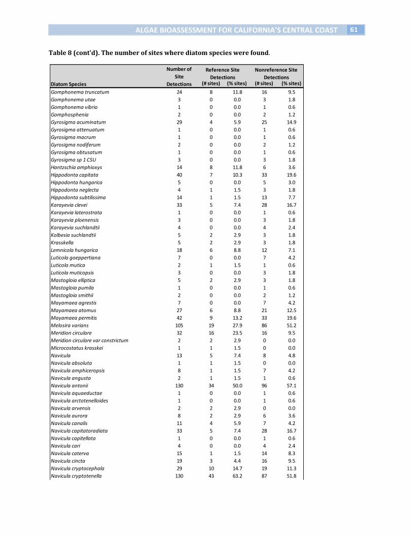
METHODS Individual diatom samples (n=291) were collected from 221 wadeable stream sites

along the California Central Coast region during the 2007, 2008, 2009 summer and

fall sampling seasons, with the exception of a small number of samples collected in

March 2008 from intermittent-type streams. The majority of sample sites were

located in a State Water Resources Control Board Region 3, which is the region

overseen by the Central Coast Regional Water Quality Control Board (Figure 3). This

region covers 29,200 square kilometers, includes approximately 3,798 kilometers of

perennial and annual streams and 378 miles of coastline (SWCRB 2002). The area

encompasses portions of Santa Cruz County on the coast, inland to the counties of

Santa Clara, Monterey, San Benito, San Luis Obispo and south to parts of Santa

Barbara County and Ventura County. Multiple north-south trending mountain

ranges populate the region, such as the Santa Cruz Mountains, Diablo Range and

Santa Lucia Range. The mountains are steep but relatively low in elevation with the

highest peaks less than 1800 m. Runoff events from the watersheds typically have

short lag times after rainfall events and high peaks due to the relative size and

steepness of the surrounding mountains (Mount 1995). Unstable rock and soil types,


such as alluvium and sandstone separate the mountains forming valleys such as the

Salinas and Santa Maria river valleys. Characterized by a Mediterranean climate, the

Central Coast contains several ecological regions. Ecoregions include Coast Range,

California coastal sage, chaparral and oak woodland, and southern and Baja

California pine-oak mountains (Omernik 1987). Climatic attributes for the region

include mild wet winters, dry hot summers and mild coastal temperatures (Sugihara

et al. 2006). Precipitation patterns vary greatly from 1700 mm mean annual

precipitation in the Santa Cruz Mountains to 250 mm mean annual precipitation the

dryer interior Salinas River valley (PRISM 2011).

Sampling Design and Sample Collection In conjunction with California State University Monterey Bay and a state-funded

project studying periphyton-based bioassessments, a team of researchers

performed fieldwork and sample collection. Staff used landscape analysis with

geographic information systems (GIS) to generate a random set of possible sample

locations throughout the region. Sites were originally identified in part by

calculating accessibility (proximity to public roads) and stream order. However,

field teams were unable to utilize some of the randomized sites. Limited

accessibility, logistical considerations and a multi-year drought constrained the

ability of teams to sample from pre-identified locations. Field crew leaders used best

professional judgment and consultation with area experts to identify the majority of

sample locations. We sampled wadeable streams with varying morphological

features and a range of ecological characteristics. This included headwater streams,

mid-valley streams, and low-valley streams with diverse land uses in the

surrounding watershed. Land uses examples such as urban areas, forests, recreation

and agricultural settings were sampled. In addition to sampling impaired test sites,

we sampled sites with minimal disturbance in the watershed such as state parks,

reserves and undeveloped regions of the Central Coast.

Field personnel used field assessment techniques consistent with methods

described in Ode (2007) and a modified algae collection method from Barbour et al.

(1999) and Peck et al. (2006) to record and collect samples. Sampling consisted of

150m reaches for streams less than 10m wide and 250m for streams greater than

10m wide. Each reach was subdivided into 11 transects of 15m or 25m respectively.

Crews collected benthic diatom samples, physical measurements and stream habitat

observations at each transect (e.g. depth, substrate type, velocity, riparian cover,

etc.). Field notes for geomorphic and riparian features included sediment deposition,

stream incision, herbivory, water clarity, channel slope (%) and evidence of fire. We

collected water samples prior to diatom collection, placed the samples on ice, and


processed for nutrient content at California State University Monterey Bay and

University of California Santa Cruz water quality laboratories.

Diatom sampling consisted of gathering the benthic substrate at each transect

location. Field crews systematically collected substrate material from the left,

middle or right of the stream channel along a transect at 25%, 50% and 75% of the

wetted width, according to SWAMP protocol and also followed by the Southern

California team (Ode 2007). The collection technique included sampling rocks or

loose substrate material at each subsection. Personnel processed diatom collection

by using a circular template (12.5 cm2) to scrape rocks with a plastic spatula and

toothbrush. Crews collected fines, sand and gravel type substrates with a similarly

sized circular cup (12.5 cm2) and spatula. In rare cases, bedrock and large boulder

sampling for diatoms was not performed. If needed, substrata in close proximity to

these substrate types were used as a proxy. In total, 137.5 cm2 was collected per

reach. Field crews rinsed the template region or the collected loose material into a

container bucket. The total liquid volume was measured (ml), transferred into a

45ml aliquot sample bottles and placed on ice. Field personnel added a solution of

glutaraldehyde within a 12-hour holding time to preserve samples. Diatom samples

were refrigerated and sent to Center for Water Sciences at Michigan State University

or to the School of the Environment at Portland State University for identification to

lowest possible taxonomic level, usually genus or species. Labs at MSU and PSU held

taxonomic harmonization meetings with the taxonomic lab at University of Colorado

that conducted the diatom work for a similar project in southern California. Labs

agreed on a set of taxonomic names that kept the finest resolution that could

reliably be identified by all three labs. Hereafter, these taxa are referred to as

operational taxonomic units (OTU). Relative abundances for OTUs were established

the Center for Water Sciences from a count of 600 individuals. Laboratory sample

processing and identification followed methods applied in the USEPA EMAP studies

and the USGS NAWQA program. Laboratory sample processing and diatom

identification was conducted by labs involved in both of the former projects.

Field and Laboratory Water Chemistry Methods

Nutrient concentrations, namely total nitrogen (TN), total dissolved nitrogen (TDN),

nitrate (nitrate + nitrate), ammonium, total phosphorus (TP), total dissolved

phosphorus (TDP), and orthophosphate were determined using a Lachat

Instruments, Inc. QuikChem 8000 Series Flow Injection Analyzer. This is a multi-

channel continuous flow analyzer that uses flow injection analysis (FIA) to allow

automated handling of sample and reagent solutions with strict control of reaction

conditions. In FIA, a fixed volume of sample is injected into a carrier stream where it


is mixed with reagents to form a color reaction. The product is measured

photometrically to determine the concentration of nutrients that reacted using the

methods in Table 2.

Table 2. Methods used for chemical analysis of water samples.

Nutrient Method Principle

nitrate + nitrite-N (SM 4500-NO3 F) Cadmium reduction

Ammonia-N (SM 4500-NH3 G) Distillation, automated

phenate

Ortho-Phosphate-P (SM 4500-P F) Ascorbic acid reduction

TN/TP USGS Method # I-4650-

03

Acid/ oxidant digestion

Dissolved TN/TP USGS Method # I-2650-

03

Acid/ oxidant digestion

Major anions (Cl-, SO2-4, NO-

3, NO-2, Br-, F-, PO3-

4) were analyzed by Ion

Chromatography (IC). FIA analysis is considered to be more accurate for NO3 than IC

analysis, but measurement of other anions adds some redundancy and provides

more conservative reference data to which changes in nutrient concentrations can

be compared.

Dissolved organic carbon (DOC) and dissolved inorganic carbon (DIC) were determined

via high temperature catalytic combustion using a Shimadzu TOC Analyzer (SM 5310-B).

Silicate was analyzed using the Lachat QuikChem Method 10-114-27-1-A. Calcium

carbonate, a measure of alkalinity, was determined by Hach Alkalinity Method 8203.

Dissolved metals were determined via ICP-MS. The low detection limits (sub ug/L)

achieved using Inductively Coupled Plasma-Mass Spectrometry (ICP-MS, EPA 200.8)

provided for the determination of dissolved metals over a wide measuring range.

ICP_MS was employed in this study to determine the concentration of the following

dissolved metals: aluminum (Al), arsenic (As), cadmium (Cd), copper (Cu), iron (Fe),

lead (Pb), nickel (Ni), and zinc (Zn). Suspended Sediment Concentrations were

determined using a filtration method, modified from the Standard Methods for the

Examination of Water and Wastewater 20th Ed, Method 2540 D. Residual sediments

were weighed on a Sartorius precision balance to establish concentrations.


Water-column and benthic chlorophyll a samples were analyzed using the

laboratory procedure specified for periphyton (EPA 445), which involves the

extraction and fluorometric determination of chlorophyll a pigments. Benthic algae

was also quantified by the combustion of organic biomass to determine the ash-free

dry mass (AFDM).

Field measures of water quality parameters at each sampling location involved

using a Hach Hydrolab with appropriate sensors for dissolved solids, dissolved

oxygen, pH, salinity, specific conductivity, water temperature and turbidity.

Quality Assurance

Implementation of the project was conducted according to the Quality Assurance

Project Plan (QAPP) approved in June 2007. The QAPP documents the sampling and

analytical methods, procedures, and requirements, training and certification,

equipment maintenance, the data quality objectives regarding precision, accuracy

and completeness, and corrective actions for quality assurance problems.

Both water quality and taxonomy data were reported in SWAMP compatible format

and submitted for inclusion in the publically available data on the California

Environmental Exchange Network (CEDEN) website (SWAMP 2010). Once this data

is uploaded by CEDEN, interested people can utilize the “data query tool” available

on the CEDEN website to access the data: http://www.ceden.org/ceden_data.shtml.

Geographic Information System Methods

We delineated watersheds for each site from the US Geologic Survey (USGS)

NHDPlus data sets which includes the National Elevation Dataset (NED), National

Hydrography Dataset (NHD), and Watershed Boundary Dataset (WBD). The

elevation data was used to determine elevation, slope, and aspect at the site.

Hydrologic stability at each site was computed from stream gage data by first

computing the ratio of the minimum reported flow divided by the maximum

reported flow for each gage included in the NHDPlus data set. From this we

developed a raster with a 4 km2 resolution by using inverse distance squared

interpolation including the closest 12 points across a radius of up to 100 km. From

this raster we developed the hydrologic stability index for each site. The mean,

minimum and maximum elevation of watersheds were determined using a USGS 30

m resolution digital elevation model (DEM). Dominant watershed rock type was

characterized from USGS digital geology maps

(http://pubs.usgs.gov/of/2005/1305/). Watershed soil permeability and depth to

bedrock were computed using the State Soil Geographic Data Base (STATSGO) from


the US Department of Agriculture, Natural Resource Conservation Service

(http://www.soilinfo.psu.edu/index.cgi?soil_data&conus&background). Climate

data were obtained for each site from PRISM (Parameter-elevation Regressions on

Independent Slopes Model) and WorldClim. Mean annual precipitation and the

minimum and maximum temperatures at sites in 2007 and 2008 were obtained

from PRISM (http://www.prism.oregonstate.edu). A number of biologically relevant

climate variables compiled by WorldClim to portray climate extremes, seasonality

and annual trends were used from available grid formats

(http://www.worldclim.org/current).

Reference/Nonreference Site Determination

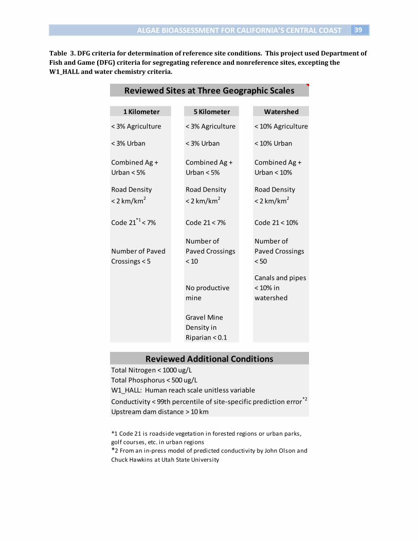
Department of Fish and Game determined conditions for assessing whether a site

was suitable as a reference site (minimal human disturbance) (Ode and Schiff 2009,

Yoder and Plotnickoff 2009). These conditions included landscape analysis,

proximity to mines and dams, number of paved road crossings, and water chemistry

criteria (Table 3).

We reviewed the 221 monitoring sites using criteria developed by the Department

of Fish and Game (DFG) and separated them into reference or nonreference sites

(Figures 4 & 5). DFG supplied the results of their GIS analysis of all sites reviewed

(2400 locations in the Central Coast) locations and with the R code for determining

reference sites. We applied all conditions recommended by DFG for determining site

suitability as a reference site, with the exception of the water chemistry parameters

(total nitrogen, total phosphorus, and conductivity) and the W1_HALL parameter,

which includes specific site inspections that were not performed by us at the time of

monitoring. As shown in Table 3, the conditions for reference site determination

included a review of the site at three geographic scales: 1 kilometer radius, 5

kilometer radius and the watershed above the monitoring site. The conditions

included maximum percent of agricultural and urban landuse, a NLCD landuse code

designating urban grasses/ roadside vegetation (Code 21), road density, number of

upstream paved road crossings, distance to a dam, gravel mine density in the

riparian zone, no productive mines within 5 km and at the watershed scale a

maximum percent of canal and pipe waterways. Although 50 monitoring sites were

not included in the DFG review, other sites close to reviewed DFG sites allowed us to

infer whether these missed sites were likely to meet the reference criteria or not.

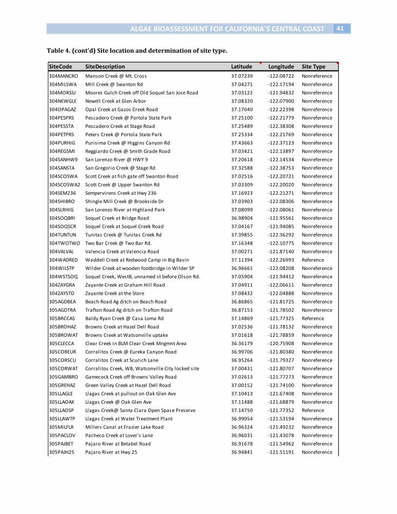
The final reference analysis identified a total of 63 reference sites and 158 non-

reference sites (Table 4).


Quantifying the Human Disturbance Gradient A metric based on the reference site classification criteria was developed to evaluate

the response of the IBI’s response to human disturbance. This metric was also used

to examine the response of individual metrics used in the final IBI. The human

disturbance gradient metric (HDG) was quantified using the proportion of

individual reference criteria that failed for a given sample site. In theory, the metric

could have ranged from 0 to 1; however, the maximum failure rate in the dataset

was 73%.

Individual reference criteria were also used to classify samples as the “best” and

“worst” with respect to site quality (i.e., level of human disturbance). These classes

were used to evaluate the responsiveness of individual candidate criteria to human

disturbance. Samples from reference sites—those that failed none of the reference

criteria—were the “best” samples. Samples from sites that failed >20% of the

individual reference criteria were classified as the “worst”. The 20% threshold was

used because it was the cutoff the produced the class size most similar to the size of

samples from the reference site pool. To help ensure the selection of responsive and

reproducible metrics for the IBI, diatom samples were treated as independent.

Index of Biological Integrity

Algae Metric Screening and Selection

A large set of possible metrics was evaluated for inclusion in the California Central

Coast multimetric algal index of biotic integrity. The initial list of metrics was

compiled based on those used in the past by others and those available as part of the

Western Environmental Monitoring and Assessment Program (WEMAP).

Methodologically problematic metrics, including those that we could not calculate

with the available data or resources, were eliminated from the candidate metric list,

(e.g. metrics based on absolute abundance). This initial screening resulted in the

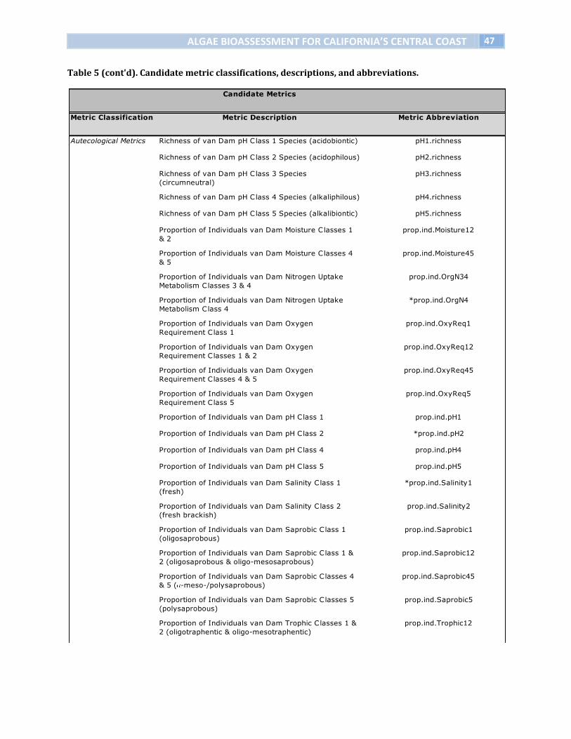
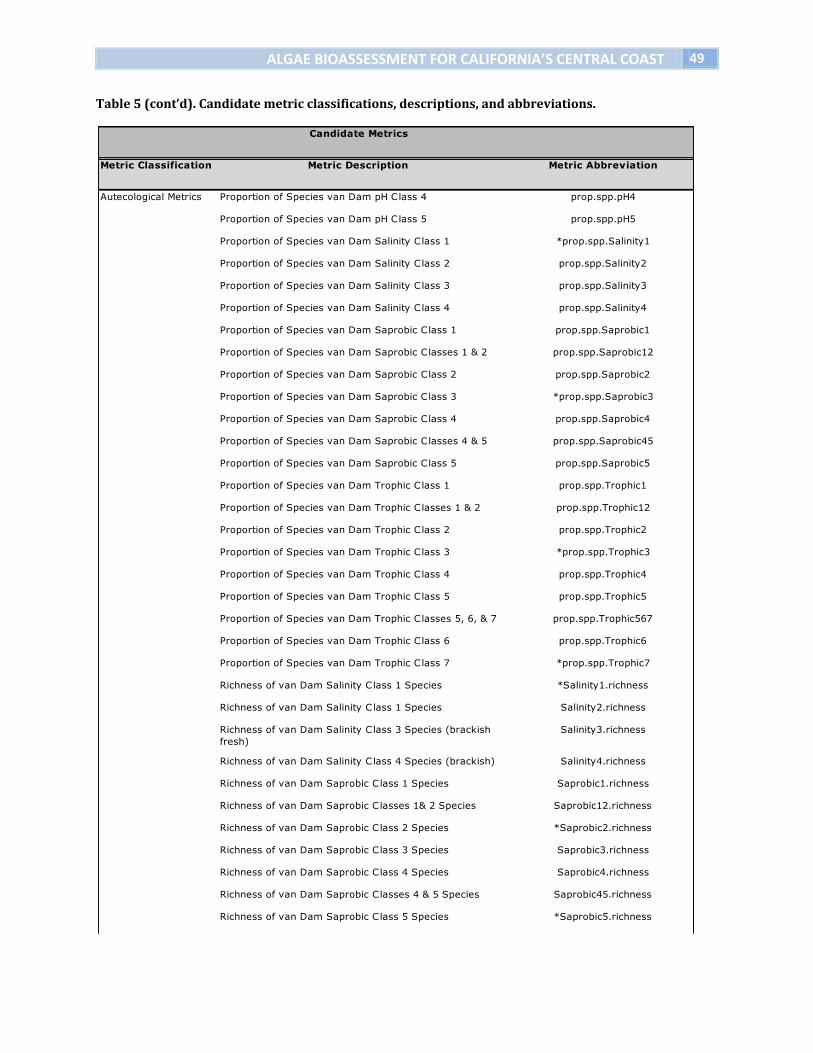
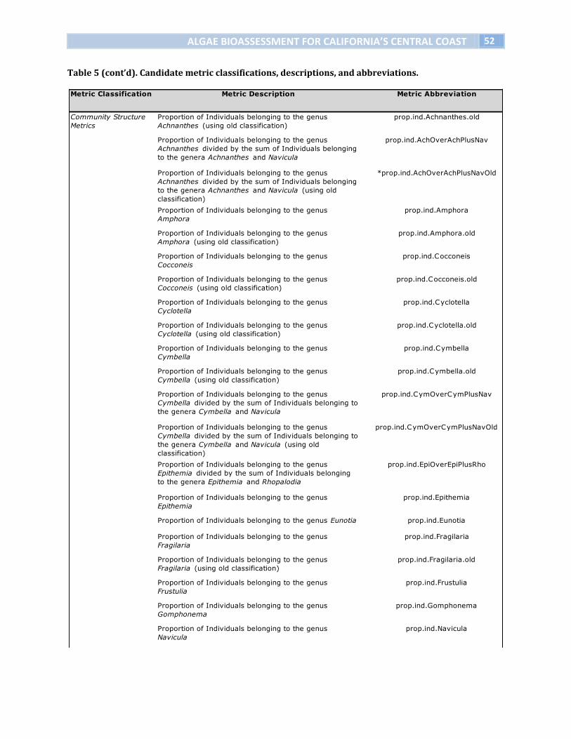
initial candidate metric list (Table 5).

Individual candidate metrics were screened using the approach of Stoddard et al.

(2008). The aim of this approach is applicability to regional and national scales

through identification of a metric set that meets 4 criteria: 1) based on a data range

with sufficient variation among sites, 2) temporal stability to allow for

reproducibility, 3) responsive to stressor gradients, and 4) relatively good

independence between metrics of the others (Stoddard et al. 2008). Metrics were

classified and evaluated for sufficient range and reproducibility. Individual metrics

were evaluated for responsiveness to human disturbance, assessed for ecological

redundancy and, when necessary, adjusted for correlation with natural gradients.


This iterative, formalized approach allowed us to quantitatively cull a long list of

candidate metrics, reducing the size to a manageable number. Furthermore, it

allowed us to maintain a compatible set of approaches with development of another

multimetric index simultaneously being developed for Southern California streams

and rivers by another research group. While the two research groups had slightly

different goals, development of an algae-based IBI for our respective regions was a

common goal.

The two teams worked together at various stages of project development in order to

coordinate methods and harmonize taxonomy to a reasonable extent. Field

protocols were developed together, using USEPA EMAP protocols as a starting point.

Extensive effort was made to ensure compatibility with existing SWAMP protocols.

Field protocols used by the Southern and Central California research teams differed

primarily in the collection, identification, and use of soft-bodied algae. The research

group from Southern California intended to make use of soft-bodied algae, using and

budgeting for methods that had not been applied in USGS NAWQA and USEPA EMAP.

In the Central California Coast, our goal was to greatly increase the number of sites

for which periphyton data were available, particularly with respect to reference

sites. In the Central Coast, we applied methods similar to those used by USEPA

EMAP for soft-bodied algae collection and processing. We identified soft-bodied

algae in several samples, but found limited utility in these data, relative to the

diatom data. Diatom identifications were harmonized with the Southern California

through a series of conference calls and meetings, resulting in a single taxonomic list

for the two regions. Index development protocols proposed by the Southern

California group were shared. Most of these protocols followed Stoddard et al. (2008)

relatively closely. Thus, we applied the peer-reviewed and published methods of

Stoddard et al. (2008) in our IBI development. Field sampling protocols, diatom

identification, and IBI development between the two regions should be highly

compatible and may even allow for the development of a single diatom-based IBI for

the two regions, should it become a priority.

Metric Classification

The first step of the Stoddard et al. (2008) approach is classification of metrics, with

preference for a classification scheme that relates inherent qualities of aquatic biota

to important elements of biotic condition. For our study, all candidate metrics were

classified into one of five ecological categories: 1) autecological preferences, 2)

community structure, 3) ecological guilds, 4) tolerance and intolerance, and 5)

production. All metrics derived from van Dam et al. (1994) were classified under

“autecological preferences”. Van Dam’s autecologies include species-level


classifications for ecological preferences in pH, salinity, nitrogen uptake metabolism,

oxygen requirements, saprobity, trophic state, and moisture. Metrics derived from

relative individual abundance, relative species abundance, dominance, evenness,

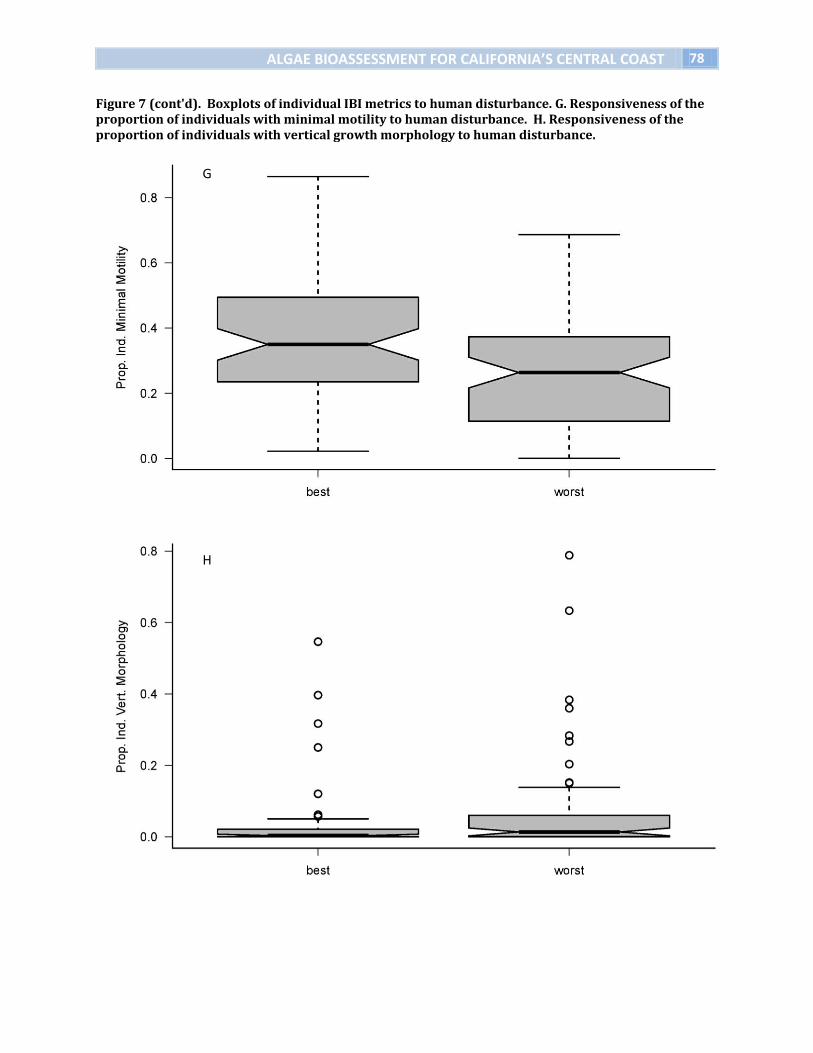
and measures of diversity were classified under “community structure”. Metrics

derived from motility and morphological classifications were included in “ecological

guilds”. Metrics pertaining to presence, dominance, and abundance were included in

community structure. All metrics derived from the pollution tolerance index

developed by Bahls (1993) were classified as tolerant and intolerant. Additionally,

tolerance and intolerance metrics were developed from our data, specific to taxa

whose abundance most effectively discriminated between sites with the least

human disturbance and sites with the greatest human disturbance. Finally, metrics

derived from measures of biomass such as chlorophyll, ash-free dry mass (AFDM),

microalgal growth and macroalgal growth were classified as “production”. Our

original intent was to develop the index of biotic integrity (IBI) using one to three

metrics from each of these ecological categories.

Individual Metric Range

To help reduce the size of the initial pool of candidate metrics, Stoddard et al. (2008)

suggests evaluating metrics for their range across sites to insure the metric can aid

in discriminating variability in conditions. Range consideration includes not only the

statistical range of a given metric, but also the exclusion of metrics that exhibit a

large proportion of similar values, such as zero, at many sites. It is important to note

that Stoddard et al. use this filter on regional and national scale in which metrics are

generally likely to exhibit sufficient range. Furthermore, they do not set specific

criteria for meeting range requirements, but note that they often remove metrics

with a range <4 or >1/3 samples with zero. Because we are working at a more

localized scale, range criteria were much more liberal. Furthermore, we were

interested not only in linear responses of metrics to stressors but also threshold

effects. Assuming that some metrics exhibit nonlinear responses to stressors, it is

possible to have metrics with small ranges but a strong ability to discriminate

between reference and non-reference sites. Therefore, metrics for which >80% of

sites were a single value, such as zero, were eliminated, as were metrics that

exhibited fewer than 4 levels. Because some metrics are based on only a few taxa,

these criteria allowed us to preserve highly responsive metrics, even if they only

exhibited different values at little more than 20% of sites.

Reproducibility

Suitable metrics should be stable within a site, responding to environmental

changes of interest with minimized variance due to sampling (Stoddard et al. 2008).


Several sites were visited at least two times and some duplicate counts were

conducted on samples collected from a single site visit, allowing us to estimate the

within site variation, in addition to the variance across sites. The signal-to-noise

ratio (S/N) was calculated for each metric by dividing the pooled site variance

(signal) by the mean within site variance (noise). All metrics with a S/N <1.5 were

eliminated. This is at the more conservative end of the <1.0 S/N criteria that

Stoddard et al. (2008) suggest for periphyton metrics.

Responsiveness

The ability to distinguish between most-disturbed and least-disturbed sites is the

most important criterion for metric selection (Stoddard et al. 2008). Welch’s two-

sample t-test was used to screen variables for responsiveness to human disturbance.

Within each metric classification, metrics with the highest absolute t-values were

considered for inclusion in the final multimetric index. Although selecting metrics

from each class may ultimately lead to a slightly less responsive multimetric index,

however doing so does help ensure that the index is ecologically representative of

multiple types of variables that best indicate conditions associated with biological

integrity. All statistical analyses were performed using R statistical software (R Core

Group 2011).

Accounting for Natural Gradients

In addition to responding to human disturbance gradients, metrics may respond to

natural gradients (Stoddard et al. 2008). Because natural gradients and human

disturbance gradients can be correlated, it can be important to adjust metrics to

help ensure that they are responding to the human disturbance gradient rather than

the natural gradient. One way to do this is to model the response of metrics to

natural gradients using only reference sites (Stoddard et al. 2008). Therefore, we

created linear regression models using only reference sites for metrics that passed

all other screening criteria and were among the most responsive metrics.

Statistically significant ( =0.05) models were then used to predict how metric

values relate to natural environmental variables such as elevation and slope.

Expected values based on environmental variability were subtracted from observed

values, resulting in a natural gradient-corrected metric. Environmentally corrected

metrics were then reevaluated for responsiveness.

Scaling, Direction-Corrections, and IBI Calculation

After individual metrics were identified, they were scaled and summed to yield an

IBI score somewhere between 0 and 100. Scaling followed recommendations by

Stoddard et al. (2008). Scaled values were calculated as follows:


Scaled metric = (x – 5th %ile of x)/(95th %ile of x – 5th %ile of x),

where x is an individual metric score at a given site.

Some metric values increase with human disturbance while others decrease. In

order to produce an IBI for which higher values represent higher biological integrity,

metric values that are positively correlated with human disturbance must first be

reversed. Subtracting values from one changes the direction of these metrics that

decrease at lower levels of human disturbance. The result is a set of 11 individual

metrics that have values near 1 at high quality sites and values near 0 for low

quality sites.

The final IBI was calculated by summing individual metric values and scaling to 100

as follows:

IBI = 100Σ(scaled metrics/11).

Count data for new samples can be entered into the spreadsheet

(CaliforniaDiatomIBICalculator.xlsx) provided to calculate the IBI score for the site

(see Appendix I). The spreadsheet scales individual metrics, makes necessary

corrections for covarying natural gradients, corrects for the direction in which

individual metrics change in response to human disturbance, and calculates the

overall IBI score. Most algae bioassessment labs can readily calculate many of the

individual metrics; however, the spreadsheet should allow IBI users to easily

calculate scores without pre-calculated metrics.

Using the IBI to Establish Biocriteria

The IBI can be used for biomonitoring and assessment. Assessment, by its nature,

places a value on levels of the multimetric (e.g., “good”, “bad”, “impaired”,

“unimpaired”, “meeting standards”, etc.). Several recommendations are made for IBI

biocriteria based on the reference site distribution and response of the IBI to trophic

status. Common distributional breakpoints, such as the median, quartiles, and

minima are generally applied to establish criteria using reference distributions.

Effects-based biocriteria are established using thresholds in the metric along an

environmental gradient, such as trophic status or human disturbance. We quantified

human disturbance as the proportion of DFG reference criteria that failed. To

quantify trophic status, we used the criteria established by Dodds et al. (1998) in

two ways. We used the TN, TP, mean benthic chlorophyll, and sestonic chlorophyll

trophic classification boundaries (Table 6). First, sites were classified as

oligotrophic, mesotrophic, or eutrophic if any one of these measures placed them


into a higher trophic state. Then we gave oligotrophic a value of one, mesotrophic a

value of two, and eutrophic a value of three. The values for all four measures (TN, TP,

mean benthic chlorophyll and sestonic chlorophyll) were summed to create a

trophic status index (TSI). Additionally, a principle components analysis-derived

trophic status index (PCA-TSI) was created by entering nutrient and algal

production measures into a principle components analysis. The first principle

component axis site scores were then used as a measure of trophic status.

Table 6. Suggested boundaries for stream trophic classifications by Dodds, Jones, and

Welch (1998). Boundaries were used to classify streams as eutrophic or mesotrophic

if one of these measures exceeded the benchmark.

Variable

Oligotrophic-

mesotrophic

boundary

Mesotrophic-

eutrophic

boundary

Mean benthic chlorophyll (mg/m2) 20 70

Sestonic chlorophyll ( g/L) 10 30

TN (mg/L) 0.700 1.500

TP (mg/L) 0.025 0.075

Various methods have been applied to quantify thresholds, some of which have been

applied to water quality criteria development. Here, we used a non-parametric

changepoint analysis (Qian et al. 2003) that acknowledges uncertainty in the

changepoint, allowing for a risk-based establishment of criteria. Using such an

approach, the median of the changepoint distribution represents a 50% chance that

the threshold has been passed. More conservative or lenient criteria may be

established using other quartiles or percentiles along the changepoint distribution.

Changepoints can be difficult to conceptualize, particularly when displayed

graphically because people are accustomed to viewing linear models. Soranno et al.

(2008) compare the relative reduction in deviance from the changepoint analysis

with R2 values from linear regression. Each describe the proportion of variation

explained by their respective model, providing for a rough comparison between

threshold and linear responses.


RIVPACS

Site Classification Based on Diatom Assemblages

Fifty-five diatom samples from the pool of reference sites were classified into

groups based on their diatom assemblages. This “calibration set” had one randomly

selected sample from each site. Any duplicate samples or samples collected during a

site revisit were placed into the “model validation set” which was later used to

assess bias in the predictive model. Diatom abundances from the calibration sites

were first transformed into presence-absence data. Assemblage dissimilarities were

calculated using the Bray-Curtis dissimilarity index. Hierarchical agglomerative

clustering was used to associate diatom assemblages using the flexible beta method

(Beta=-0.6).

The dendogram resulting from the analysis was then pruned to produce site classes

of similar diatom assemblages. Although pruning level is subjective, the goal is to

organize sites into classes of sufficient dissimilarity and size. Lengths of branches in

the dendogram are proportional to the variance in assemblage dissimilarities

explained. Therefore, pruning branches that are long rather than short helps

maximize dissimilarity between groups. Additionally, it is important that each class

resulting from pruning should be represented by a sufficient number of sites

without being so overly conservative as to create large, heterogeneous classes. Our

pruning level was chosen to maximize distance between classes with a target class

size between ten and thirty sites. Thus, based on the size of our calibration set, the

number of classes would fall somewhere between two and five.

Predictor Variables

RIVPACS-type models use environmental variables to predict class membership,

thus establishing expected conditions at a site. Because predictor variables for these

models are used to infer biological assemblages if a site were experiencing minimal

human disturbance, it is important that the predictor variables are influenced little

by human activities at the landscape scale being assessed. Therefore, measures of

climate, geologic, and geographic characteristics are ideal, whereas measures

related to water chemistry or correlated with streamside human activity should be

avoided. Furthermore, variables that can be derived from GIS allow expected

conditions to be calculated for every stream reach within the region without

collecting field data.

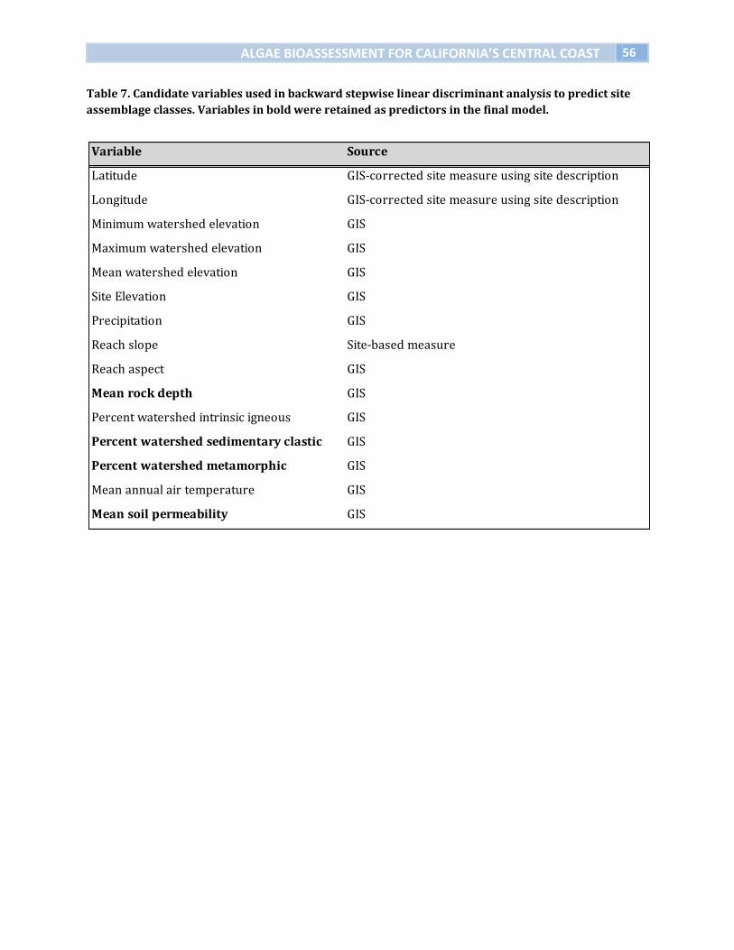
Approximately fifty potential predictor variables were screened for redundancy,

high correlation with other variables, and sufficient range. This process resulted in


fifteen candidate variables (Table 7) that were used to construct a predictive model

for assemblage class membership.

Predictive Model

Backward stepwise linear discriminant analysis was used to construct a predictive

model for diatom assemblage class membership in the calibration set. This

association of environmental variables with reference clusters allows the model to

make future predictions for expected taxa at a given test site. The predictor

variables were used to develop the OE metric by establishing a strong association to

biological groups at reference sites and comparing those environmental

characteristics at test sites to make expected taxa predictions. This stepwise

approach resulted in the same final model as the best-subset routine used by others

(e.g., Van Sickle et al. 2006). More in-depth discussions of the statistical steps for

RIVPACS model construction are described elsewhere (Wright et al. 1984; Moss et al.

1987; Kaufman and Rousseeuw 1990; Wright 1995; Marchant et al. 1997; Hawkins

et al. 2000; McCune and Grace 2002); however a basic outline is provided by the

following steps:

Step One: Organize reference sites. One diatom sample was randomly selected from

each reference site to develop the calibration set (n=55). These sites were used to

develop the diatom assemblage classes used in the predictive model. All remaining

duplicate samples from reference sites were used for the validation set (n=17). The

validation set was used to evaluate the accuracy of the predictive model. We

evaluated model performance by generating an OE score for the calibration sites,

and for the validation sites and reviewed how close to one, or high biological

integrity, they scored (Hawkins et al. 2000; Van Sickle et al. 2006). One measure of

good model performance is O/E scores at validation sites of one or very close to one.

Step Two: Biological clustering. A first step in building the model involved biological

classification of sites containing similar assemblages of diatoms at the species or

variety level. Reference sites were clustered into groups containing taxonomically

similar assemblages by using cluster analysis. In later steps, these reference clusters

provided the basis for associating environmental variables to biological groups in

order to create a predictive model. The predictive model was developed by

clustering reference sites into taxonomically similar assemblages and determining

natural environmental predictor variables that related group members. Use of the

RIVPACS method assumes that species composition and abundance within

assemblages varies and conforms along changing environmental gradients and

settings (McCune and Grace 2002). We started by removing rare species (those


occurring at fewer than 5% of the reference sites) prior to the biological clustering

in order to decrease the “noise” from rarely occurring species (Hawkins et al. 2000,

McCune et al. 2000). After clustering, we added the previously removed taxa back

into the data used for final O/E predictions. These clusters of self-similar

assemblages were used to find predictor variables strongly associated with the

cluster groups in order to predict assemblages along natural gradients and verify

these at test sites. We accomplished this by using discriminant analysis. These

strongly associated predictor variables would be used to predict expected taxa at

degraded sites.

To achieve the clustering of sites into groups based on their taxonomic composition,

we created a hierarchical dendrogram using an agglomerative nesting technique

(AGNES). The agglomerative nesting constructed a tree-like dendrogram, which

related biologically pairs of individual sites at one end and built upward to relate

branches to a top cluster containing all sites (Kaufman and Rousseeuw 1990;

McCune and Grace 2002). A flexible, unweighted, pair-group average method

(UPGMA) used presence-absence data in conjunction with a Bray-Curtis

dissimilarity coefficient to determine ordination distances (McCune and Grace 2002;

Van Sickle et al. 2006). Calibration sites were linked with a flexible-β method (β=

−0.6), where β = 1-2α (Hawkins et al. 2000; McCune and Grace 2002; Van Sickle et al.

2006). To reflect an ordination strategy similar to Ward’s linkage method (Ward

1963), which minimized sum of square errors derived from Euclidean distances.

Once the dendrogram was created, we “pruned” the tree to establish cluster groups.

Cluster groups were formed by creating a cut-off point on the dendrogram to

maximize the formation of taxonomically self-similar groups with 10-30 sites per

cluster (Hawkins et al. 2000).

Step Three: Predictive modeling with environmental variables. This portion of the

model construction associated environmental characteristics with previously

established biological clusters. After model construction, this step enables the model

to predict reference assemblages at any site based on similar environmental

characteristics. In order to identify the environmental predictor variables

establishing membership of a test site in one of the taxonomic groups identified in

the cluster analysis above, we used discriminant analysis. Linear DA is analogous to

multiple regression analysis, as it employs predictor variables to determine the best

fitting classification of a sample set to a group (Williams 1983). Linear DA was used

to identify predictors with the strongest association to the biological clusters to

classify and group the calibration sites to match the dendrogram of biological

clusters (Wright et al. 1984; Marchant et al. 1997; Hawkins et al. 2000; Van Sickle et


al. 2006). We used backwards stepwise linear discriminant analysis to select the

best subset of predictor variables. This approach resulted in the same model

produced by the best-subset algorithm applied by others (Van Sickle et al. 2006;

Poquet et al. 2009).

Step Four: Group membership probability and taxon frequency. This step determined

the probability of any site belonging to a reference group and was used to generate

expected taxa. DA had a dual purpose for model development by first grouping the

reference site data (Step 3 above), and second by assigning the probability of any

site (test or reference) being a member of any one of the classified reference groups

(Pj). DA was used to accomplish this by maximizing the separation between a fixed

number of groups (previously discerned from biological clusters) along an

orthogonal scale in ordination space and calculated the probabilities of each site

belonging to each group (Mahalanobis distance in multidimensional space between

each site and the centroid of cluster groups) (McCune and Grace 2002; Poquet et al.

2009). A frequency of occurrence for each taxon (k) was established within each

cluster group (g). The average proportion of each taxon within the member-

established reference cluster groups (gj,k) was calculated (Marchant et al. 1997).

Step Five: Probability of capturing observed taxa at reference sites. Final taxa counts

were established using statistical operations to generate the expected diatom

assemblages. To facilitate prediction of taxa at each site, the program summed the

product of gj,k and Pj to determine the ‘probability of capture’ (PC) for each taxon. PC

uses the final set of selected predictor variables and predicts the expected taxa for

all sites. For this investigation, a probability of capture (PC) level of 0.5 was used as a

starting point for predictive model use following variable selection. By applying the

model constructed using the calibration set to the validation set, bias in O/E

estimates can be assessed. PC level was adjusted to a level that was sensitive but

unbiased. A PC value of 0.1 was eventually selected for the model.

Step Six: Expected prediction and OE calculation. The final model construction step

calculated total expected taxa for a site and produced the observed to expected (O/E)

metric. The O/E score was then used as a measure of biological integrity at each site.

Observed taxa from the test sites were counted only if the species were identified at

reference sites. Species observed but not part of the expected lists were not

incorporated into the OE metric. The procedure calculated observed taxa (O) at all

the sites by summing the total of each expected taxon observed in the actual sample

data. The outcome of the predictive models was an O/E score for each site. The O/E

score was used to determine degradation by establishing and upper baseline score


and lower baseline score for O/E values. O/E scores near one were identified as

non-degraded. OE scores outside the upper and lower bands were identified as

degraded. We deemed a site degraded based on the 0.10 and 0.90 percentiles of

calibration O/E results (Van Sickle et al. 2005). While traditionally, RIVPACS models

use only lower bounds, Van Sickle et al. also incorporate the upper bounds. For

diatoms this may be particularly important because low nutrient regions often

exhibit an increase in diatom species richness as a result of nutrient enrichment.

Results and Discussion

Taxonomical Results

Benthic samples were sent to two different labs for identification of taxa: Dr. Jan

Stevenson at Michigan State University (MSU) and Dr. Yangdon Pan at Portland

State University (PSU). Occasionally samples from the same site and collection date

were evaluated at both labs for comparison of results. Taxonomic evaluation of

samples sent to MSU were evaluated for diatoms and sometimes soft algae, whereas

samples sent to PSU were evaluated solely for diatoms. All diatom counts were

harmonized between MSU, PSU, and the Southern California project’s taxonomic lab

at the University of Colorado. A single list of California diatom taxa was created

through several conference calls and meetings. Taxa that could be reliably

distinguished by all three labs were retained in counts analyzed. In some cases, the

same entity was given different names by labs. After discussion and analysis, labs

agreed upon a single taxonomic name. In rare cases that diatom taxa were not

differentiated similarly among labs, taxa were lumped into a single operational

taxonomic unit (OTU) for data analysis. All taxa that were not identified to the level

of genus were eliminated from the data set. Taxa identified to the level of genus, but

not species, were included and counted as separate species; thus the total number of

species may be slightly over represented. Taxonomic identification of samples from

212 sites, found a total of 501 different diatom species representing 85 genera were

collected in Central Coast wadable streams. The number of species detected at the

56 reference sites was 347 and at the 156 nonreference sites was 453 (Table 8).

From 39 sites, a total of 37 soft algae species representing 25 genera were identified

in benthic samples. Of the soft algae, 13 species were found at the 8 reference sites

whereas 36 species (all but 1) species were found at the 31 nonreference sites

(Table 9


Metric Screening During initial screening of the potential metric list, all potential metrics based on

absolute abundance were removed. These metrics require an estimate of cell

densities from the original streambed or riverbed, which was not available for much

of our data. Furthermore, the method by which these estimates are made can be

biased, based on the method applied to estimate diatom densities (Alverson et al.

2003).

Initial screening led to a list of 250 candidate metrics. Classification is the first step

in determining an IBI (see Methods: Metric Classification). Classification of these

metrics into environmentally relevant groupings resulted in 10 metrics being

classified as tolerant or intolerant, 21 as ecological guild, 94 as community structure

metrics, 117 as autecological, and 8 as production metrics (Table 10).

Several metrics were eliminated from candidacy for failing the range test. Metrics

exhibited inadequate range if either 80% of their measures were of a single value or

if there were fewer than 4 levels measured in the dataset. These metrics included

the autecology variables: proportion of individuals that are van Dam’s pH Class 1,

proportion of individuals that are van Dam’s pH Class 2, Richness of van Dam’s

Moisture Class 5, proportion of species belonging to van Dam’s Moisture Class 5,

species richness of van Dam’s pH Class 1, species richness of van Dam’s pH Class 2,

proportion of species belonging to van Dam’s pH Class 1, and proportion of species

belonging to van Dam’s pH Class 1. Community structure metrics with inadequate

range included proportion of individuals belonging to the genus Achnanthes,

proportion of individuals belonging to the genus Eunotia, proportion of individuals

belonging to the genus Frustulia, species richness within the genus Achnanthes,

proportion of species belonging to the genus Achnanthes, species richness within the

genus Eunotia, proportion of species belonging to the genus Eunotia, species

richness within the genus Frustulia, proportion of species belonging to the genus

Frustulia, species richness within the genus Rhoicosphenia, proportion of individuals

belonging to the genus Achnanthes divided by the sum of the proportion of

individuals belonging to the genera Achnanthes and Navicula, and proportion of

species belonging to the genus Achnanthes divided by the sum of the proportion of

species belonging to the genera Achnanthes and Navicula,. All tolerance/intolerant

and ecological guild metrics met range criteria.

A number of metrics exhibited signal-to-noise ratios below 1.5, failing the

reproducibility criterion. These metrics are indicated in Table 5 by an asterisk in


front of the abbreviated name. Additionally, all production metrics failed this

criterion; so all production metrics were excluded from the IBI.

Metrics that met other screening criteria were then evaluated for responsiveness to

human disturbance. T-statistics from Welch’s two-sample t-test were used to

quantify the ability of each candidate metric to distinguish between the best and

worst sites (see Quantifying the Human Disturbance Gradient above). The two or

three metrics with the highest absolute value for the t-statistics were evaluated for

significant correlations with the two environmental factors that we felt would most

likely confound responsiveness to the human disturbance gradient: elevation and

slope because agriculture, urbanization, and residential development tend to be

more concentrated in valleys. Only two of the top metrics were significantly

correlated with one of these non-anthropogenic environmental variables (Table 10).

The weighted pollution tolerance metric was positively correlated with slope and

the proportion of species belonging to the genus Epithemia was positively

correlated with elevation. When weighted pollution tolerance was corrected for

slope (see section "Accounting for natural gradients"), its t-statistic dropped below

that of the proportion of individuals belonging to pollution tolerance class 3, which

was not significantly correlated with slope or elevation. The proportion of species

belonging to the genus Epithemia was elevation-corrected and retained for use in

the IBI. Additionally, metrics that were biologically correlated (as opposed to

statistically correlated) were considered redundant because they provide the same

information. If two or more metrics were redundant, only the metric with the

highest absolute t-statistic was retained. Eleven metrics (three autecological, three

community structure, three tolerance/intolerance, and two ecological guild metrics)

were retained for the final IBI. Each of these metrics responded significantly to

human disturbance (Table 10, Figures 7A-7K).

Diatom Index of Biotic Integrity (IBI) for wadable streams and rivers of California's Central Coast The multimetric algal index of biotic integrity contained eleven individual metrics.

Boxplots of each IBI metric for the best and worst sites (see “Quantifying the Human

Disturbance Gradient”) are displayed in Figure 7 (A-H) and results of Welch's t-test

in Table 10. These individual metrics were scaled as described in the methods and

summed, resulting in a single value for each sample. While the metric could

theoretically range from 0 to 100, the observed range was 17.28 to 92.57. The

distribution of IBI values across all samples was unimodally distributed, with a

median value of 55.04.


Worst sites had higher median values for presence of species in all three

autoecological metrics indices that distinguished best and worst sites on the Central

Coast: proportion of species in van Dam's trophic class 5, abundance-weighted

average of van Dam's salinity score, and proportion of species in van Dam's oxygen

requirement class 5.

It can be difficult to classify diatoms according to a positive or negative response to

nutrients, and there may be local, regional or continental scale differences

(Patapova and Charles 2005). Van Dam (1994) describes 7 trophic states, where

species tolerant of high nutrient levels are categorized in the eutraphentic level

(Figure 7A). Whereas US national NAWQA metrics classify the common species

Achnanthidium minutissimum as a low-nutrient indicator, van Dam’s classification

from European waters places it in the trophic level indifferent to nutrients

(Potapova and Charles 2005). In our study, A. minutissimum was present in equal

percentages of reference and nonreference sites (68%). For the Central Coast, using

the van Dam class 5 metric, we observed a significant difference between best and

worst sites on the Central Coast (t-stat = 4.9).

A second metric from this classification was the weighted average of the van Dam

salinity score, which had similar medians for best and worst sites. However there

was a greater range of species in the worst sites and a significant difference between

best and worst sites (t-stat = 4.3). Van Dam (1994) classifies oxygen requirements

into 5 levels, with very low oxygen requirements at about 10% saturation. On the

Central Coast, the proportion of Van Dam species with very low oxygen

requirements were more prevalent in worst sites (Fig. 4.B) and the t-test showed

strong discrimination between best and worst sites (t-stat = 4.0).

In the community structure metric class, the three metrics that passed all the tests

were related to species dominance (Figures 7D, 7E and 7F). The two species

richness indices were correlated with these metrics and the not included in the final

IBI because the higher t-statistic was associated with the dominance metrics. The

final IBI metrics were the proportion of species belonging to the genus Epithemia (t-

stat = -6.0), the proportion of species belonging to the genus Amphora (t-stat = 5.4),

and the proportion of individuals belonging to the genus Achnanthes divided by the

sum of individuals belonging to the genera Achnanthes and Navicula using genera

from Kramer and Lange-Bertalot (1986, 1988, 1991a,b) rather than the current

taxonomically accepted genera (t-stat= -5.3). The two species richness indices were

for the genera Epithemia and Amphora, with Amphora having greater species

richness in worst sites (t-stat = -6.1) and Epithemia in best sites (t-stat = 5.4). The


most prevalent species on the Central Coast was Amphora pediculus, observed at

199 out of 236 sites (84%) and present at 72% of reference sites and 89% of

nonreference sites. A total of 8 different Amphora species were identified and each

was present at a higher percentage of nonreference sites compared with reference

sites (Table 8). We observed 3 species belonging to the Epithemia genus and in each

case, these species were, by contrast, more likely to be found at reference than at

nonreference sites. The species Epithemia adnata was present at 47% of reference

sites and only 19% of nonreference sites. Epithemia contain endocellular

cyanobacteria, making them capable of nitrogen fixation (Floener and Bothe 1980).

This may explain their presence in reference conditions with generally lower

concentrations of total nitrogen and nitrate as compared with higher concentrations

in nonreference sites (Fig. 13).

Two metrics from the ecological guild class were good indicators of site quality on

the Central Coast: the proportion of individual with minimal motility (Fig 4.G, t-stat

= -4.4) and the proportion of individuals with vertical morphology (Fig. 4.I, t-stat =

3.2). Ecological guild is a useful classification because diatom behaviors are distinct

and predictable within guilds along a nutrient and disturbance gradient (Passy

2006). Differences between guilds include motility and profile (Passy 2006). A

higher proportion of individuals with minimal motility was seen at best sites and a

higher proportion with vertical morphology at worst sites. Motile diatoms can move

on and around streams with high sedimentation because of their raphe and may

have increased abundance at locations with a silty bottom (Stevenson and Bahl

1999, Wang et al. 2005). On the Central Coast, motility may be less important in best

streams, i.e. those more removed from human disturbance and less likely to have

associated sediment, and at higher elevations where sediment is less likely to

accumulate. Diatoms with a more vertical profile are susceptible to disturbances in

stream hydrology whereas prostate diatoms are less sensitive to hydraulic

disturbance (Stevenson and Bahl 1999). The higher proportion of individuals with

vertical morphology at more disturbed sites on the Central Coast may be related to

the greater control exercised over preventing hydraulic disturbance in these areas

in order to use surrounding lands for human purposes, ie. agriculture and

urbanization.

From the tolerance/intolerance metric class, the three indices were indicative of site

quality on the Central Coast: the proportion of individuals classified as California

Central Coast most sensitive, the proportion of individuals classified as California

Central Coast most tolerant, and the proportion of species classified as Bahl's

pollution tolerance class 3. Sensitive species are by definition those present and


abundant in reference streams, whereas tolerant species prevail in more impaired

streams. Bahl (1993) developed pollution tolerance classes for diatoms observed in

Montana based on Lange-Bertalot's classes. Bahl's pollutions tolerance class

included three groups: (1) most tolerant, (2) least tolerant and (3) sensitive. The

species classified as most tolerant for California's Central Coast were Amphora

pediculus, found in 89% of nonreference sites (Table 8), and Navicula gregaria found

in 83% of nonreference sites. The species classified as least tolerant for California's

Central Coast were Encyonopsis microcephala (9% of reference sites), Epithemia sore

(23% of reference sites), Gomphonema acuminatum( 9% of reference sites),

Gomphonema pumilum (14% of reference sites), Navicula canalis (4% of reference

sites), Navicula cryptotenella (52% of reference sites), Navicula cryptotenelloides (2%

of reference sites), and Navicula radiosa (15% of reference sites). The criteria for

inclusion in the two California Central Coast-specific metrics were a positive S/N

and a statistically significant difference in abundance between the highest quality

and least quality sites. These criteria are quite liberal and did lead to the inclusion of

three relatively rare species in the intolerant metric. A larger set of reference sites

may be necessary to determine whether these are truly intolerant species. Because

of their rarity, the IBI is unlikely to be substantially affected by their removal.

Multimetric biotic indices are a recent approach used in biological monitoring of

streams to aid resource managers in assessing biotic condition and identifying

stressors (Hill et al. 2003, Wang et al. 2005). Karr and Chu (2000) describe

multimetric biological indices as a stalwart means for diagnosing, minimizing and

preventing river degradation. Wang et al. (2005) asserts that diatom biotic indices

are also valuable toward aiming restoration efforts at protecting resources and

restoring the base of the food chain, i.e. the primary producers in streams. Others

have criticized multi-metric indices because they are a greatly simplified single

number representing a complex set of relationships and because there is poor

understanding of their distribution (Suter 1993, Norris 1995). The advantage of

single number index is that it provides for quick assessment and may aid resource

managers in focusing their efforts in managing a large scale region.

The Central Coast IBI was negatively correlated with the human disturbance

gradient metric (Pearson Correlation = -0.61; Figure 8). The IBI effectively

distinguished between sites with the highest human disturbance and the sites with

the lowest human disturbance (t = 9.2953, df = 144.201, p < 0.001; Figure 9). Only 7%

of sites in the “worst” human disturbance class had IBI values greater than the first

quartile of the “best” human disturbance class and only 6% of sites in the “best”

class had values below the third quartile of the “worst” class. Reference site IBI


values (mean = 50.96) were also significantly higher than IBI values for the full set

of nonreference sites (mean = 66.51) (t = -9.6364, df = 131.277, p < 0.001).

Identifying Potential IBI-based Water Quality Criteria

Distribution-based water quality criteria often use quartiles or percentiles of data

distributions from the set of reference sites. Following this approach, the first

quartile of the reference site IBI distribution can be applied as the cutoff between

sites with “good” and “fair” scores, and the minimum value of the references site IBI

distribution (excluding statistical outliers) can be applied as the cutoff between “fair”

and “poor” scores (Figure 10). Using these values, IBI scores >58 are “good”, IBI

scores ranging from 48 to 58 are “fair”, and IBI scores <48 are “poor”. Using these

reference-based distribution-derived criteria, 29% of nonreference sites have good

IBI scores, 32% have fair IBI scores, and 39% have poor IBI scores.

Examining response of the IBI to the human disturbance gradient revealed a

negative linear relationship with no apparent threshold (Figure 8) and thus, a

reasonable biocriterion could not be derived. The relationship the IBI to trophic

status, however, revealed several potential numeric thresholds that could be used to

develop biocriteria. The IBI did exhibit a threshold response to trophic status,

however. Sites with lower IBI scores had a higher probability of being eutrophic; the

median threshold value was 66.47 (Figure 11A). A threshold was also observed with

TSI; sites below the median of 41.57 had higher TSI values than sites above the

median threshold value (Figure 11B). A third measure of trophic status was also

used. Principle components analysis was used to reduce the dimensionality of the

chemistry matrix. The first principle component axis was highly correlated with all

measures of nitrogen and chlorophyll and thus may be thought of as a measure of

trophic status. Using this PCA-derived TSI, a strong threshold exists around an IBI

score of 35 (Figure 12). Like the reference distribution approach, the effects-based

approach suggests upper and lower breaks that provide potential boundaries

between good, fair, and poor IBI scores. Using the median value, of the eutrophic

threshold, good IBI scores would be those above 66.47. This would mean that many

reference sites would not qualify for good IBI scores. A less stringent approach

would be to use the lower quartile of the threshold distribution. This would place

the boundary at 51.49, which is closer to the break suggested by the reference

distribution approach. At the lower end, median thresholds based on TSI responses

were 35.45 and 41.57. These are lower than the boundary suggested by the

reference distribution approach. Using the upper quartile on these threshold

distributions has little effect, since these thresholds were so strong. Using the


effects-based boundary would reduce the number of “poor” sites and increase the

pool of “fair” classifications in the nonreference sites.

Application of the IBI to Recommend Effects-based Criteria In addition using the IBI to establish quantitative biocriteria, we used it as a

response variable to demonstrate its application in effects-based criteria for

nutrients, i.e. using change point analysis to establish the thresholds. Change point

analysis attempts to estimate the point in a series of observations where statistical

properties (typically the mean and variance) of a response variable indicate a

structural change in an ecosystem (Qian et a. 2003). Thresholds along

environmental gradients are logical locations to establish water quality criteria for

nutrients. These approaches are demonstrated for total nitrogen [TN (mg/L)],

nitrate as nitrogen [NO3-N (mg/L)], and total phosphorus [TP (mg/L)].

The median threshold value for response of the IBI to TN was 0.584 mg/L (Figure

13A), a significantly lower threshold than those produced using the algal production

endpoints suspended chlorophyll (median = 1.646 mg/L; Figure 14A) and benthic

chlorophyll (median = 2.340 mg/L; Figure 14B). The algal biomass endpoint

thresholds were also weaker than the threshold with IBI.

The median threshold value for response of the IBI to TP was 0.046 mg/L (Figure

13B). The median IBI threshold was roughly half the median threshold using

suspended chlorophyll as the endpoint (median = 0.088 mg/L; Figure 15A). The

threshold produced using benthic chlorophyll as the endpoint was weaker but had a

similar value to that using the MIABI endpoint (median = 0.0391 mg/L; Figure 15B).

The nitrate-IBI threshold had a median value of 0.298 mg/L (Figure 16). This is a

value much lower than the 1.0 mg/L proposed screening criterion to protect aquatic

life uses (Worcester et al. 2010). At a nitrate concentration of 1.0 mg/L, there is an

86% chance that the threshold has been surpassed, leading to lower average IBI

scores. Despite the appearance of a linear relationship when the x-axis is

transformed, the relative reduction in deviance (0.22) for the changepoint analysis

is larger than the R2 (0.21) for the linear model using log-transformed nitrate.

Histograms comparing nitrogen at reference and nonreference sites show not many

nonreference sites have high total nitrogen or nitrate (>10 mg/L); however no

reference sites had high total nitrogen or nitrate (Figure 17).

Qian et al. (2003) recommend that a change point may sometimes be better

estimated as a small range rather than a single value by applying Bayesian or

nonparametric changepoint analysis. Here, we have applied the nonparametric


approach and show the median as a solid line, along with the 5th and 95th percentiles

as dashed lines (Figures 11-15). Thus values within this range may be considered

for use as effects based biocriteria in the Central Coast region based on the risk that

managers are willing to take in surpassing the threshold at various levels of nitrate. .

The threshold represents a nitrate value above which IBI values are, on average,

significantly lower than below. The mean IBI value below the median nitrate

threshold (0.2980 mg/L) is significantly higher than above (mean below = 58.4,

mean above = 42.7, t = 9.2841, p < 0.0001).

RIVPACS

Agglomerative hierarchical clustering followed by dendogram pruning resulted in

three assemblage classes in the calibration set (Figure 18). Class 1 was the largest

with twenty-one sites, class 2 contained 20 sites and class 3 contained 14 sites.

Backwards stepwise linear discriminant analysis resulted in a predictive model with

four GIS-derived geological variables that resulted in the best predictions of diatom

class membership. These variables were mean rock depth, percent sedimentary

clastic, percent metamorphic, and mean soil permeability. The average mean rock

depth for diatom classes 1-3 were 59.0 m, 67.7 m, and 57.2 m, respectively. Percent

sedimentary clastic averages were 69%, 50%, and 41%. Percent metamorphic

averages were 12%, 4%, and 19% (Figure 19). Mean soil permeabilities were 3.8

in/h, 3.4 in/h, and 4.4 in/h.

ANOVA using Helmert contrasts was used to test for the significance of O/E values

for calibration, validation, and test sets (Figure 20). O/E values for the calibration

set were not significantly different from 1.0 (t=0.319, p=0.750), with a mean of

1.010 and a standard deviation of 0.245. Validation O/E values were not

significantly different from the calibration set (t=-0.026, p=0.980). Despite a

relatively high variance in the calibration O/E set, test sites composed of all

nonreference sites had O/E values that were significantly lower than the reference

sites making up the calibration and validation sets (t=-2.695, p=0.007; ANOVA

F=4.435, df=2,283, p=0.0127).

The 10th and 90th percentiles of the calibration set can be used as impairment

benchmarks (Figure 21). For our calibration set O/E distribution, these values are

0.66 and 1.32. Sites with O/E below 0.66 may be impaired. Likewise, sites with O/E >

1.32 could be of concern. (Figure 19). Fourteen percent of nonreference site samples

had O/E values less than 0.66 and 4% had O/E values above 1.32.


Conclusions A multimetric algal index of biotic integrity (IBI) was developed for the California

Central Coast. Hundreds of individual candidate metrics were classified into

ecological classes and screened for adequate range, reproducibility, and

responsiveness. Top metrics were selected and incorporated into the final

multimetric index. The IBI responded linearly along the human disturbance gradient

and reference sites had significantly higher IBI scores than nonreference sites.

The IBI reference distribution and response to trophic status provide convenient

boarders between “good”, “fair”, and “poor” IBI scores. The reference distribution

first quartile and minimum were used to establish boundaries. Scores less than 48

are “poor”, 48-58 are “fair” and greater than 58 are “good”. Effects-based boundaries

were more extreme than those based on the reference distribution, expanding to 35

to 42 at the low end and 66 at the high end. Effects-based boundaries suggest that

many reference sites are in “fair” condition and that a higher proportion of

nonreference sites are in “fair” condition, rather than “poor”. Thus, the reference-

based boundaries seem more reasonable.

Threshold responses of the IBI to nutrients were observed. These thresholds were

stronger than those observed for nutrient-biomass thresholds. Using the median of

nonparametric changepoint distributions to quantify thresholds suggest a total

nitrogen (TN) criterion of 0.584 mg/L and a total phosphorus (TP) criterion of 0.046

mg/L. These numbers are slightly higher, but not unlike the TN and TP criteria

suggested by the USEPA for nutrient level III ecoregion 6. Using the 25th percentile

of the reference site distribution for these water chemistry measures, criteria of 0.5

mg/L for TN and 0.030 mg/L for TP (USEPA 2000). The median threshold value for

NO3-N was 0.298 mg/L. This would likely be considered a very low nitrate criterion

in the region. The nonparametric changepoint distribution suggests that there is an

86% chance that the threshold has been surpassed at the proposed screening

criterion to protect aquatic life uses. These results provide direct evidence that

actual harm to aquatic life uses may be observed above the 1.0 mg/L criterion.

The RIVPACS-type model was not as precise as desired, but nonreference sites still

had O/E values significantly lower than those at reference sites. O/E can be applied

as a metric to assess biological integrity. Large deviations from O/E=1.0 can indicate

impairment. For these data, only 18% of nonreference sites are impaired if applying

the 10th and 90th percentiles of the calibration O/E as biocriteria.


Table 3. DFG criteria for determination of reference site conditions. This project used Department of

Fish and Game (DFG) criteria for segregating reference and nonreference sites, excepting the

W1_HALL and water chemistry criteria.

1 Kilometer 5 Kilometer Watershed

< 3% Agriculture < 3% Agriculture < 10% Agriculture

< 3% Urban < 3% Urban < 10% Urban

Combined Ag +

Urban < 5%

Combined Ag +

Urban < 5%

Combined Ag +

Urban < 10%

Road Density

< 2 km/km2

Road Density

< 2 km/km2

Road Density

< 2 km/km2

Code 21*1 < 7% Code 21 < 7% Code 21 < 10%

Number of Paved

Crossings < 5

Number of

Paved Crossings

< 10

Number of

Paved Crossings

< 50

No productive

mine

Canals and pipes

< 10% in

watershed

Gravel Mine

Density in

Riparian < 0.1

Total Nitrogen < 1000 ug/L

Total Phosphorus < 500 ug/L

W1_HALL: Human reach scale unitless variable

Conductivity < 99th percentile of site-specific prediction error*2

Upstream dam distance > 10 km

Reviewed Sites at Three Geographic Scales

Reviewed Additional Conditions

*1 Code 21 is roadside vegetation in forested regions or urban parks,

golf courses, etc. in urban regions

*2 From an in-press model of predicted conductivity by John Olson and

Chuck Hawkins at Utah State University


Table 4. Site location and determination of site type. A total of 221 sites were sampled. Using DFG

criteria for reference site determination, except for water chemistry and W1Hall, sites were typed

into reference (sites) and nonreference (sites).

SiteCode SiteDescription Latitude Longitude Site Type

200BEABEA Beardsly Creek @ Beardsly Rd 37.19543 -122.00260 Nonreference

200COYCOC Coyote Creek @ Cochrane Rd. 37.16508 -121.63244 Nonreference

200COYCOI Lower Coyote Creek at Coit Rd. 37.12618 -121.48072 Reference

200EASHEN East Fork Coyote Creek @ Bear Mountain Road 37.19393 -121.46813 Reference

200GUAHIC Guadalupe Creek @ Hicks Rd 37.18047 -121.87250 Nonreference

200HERALA Herbert Creek @ Almitas Rd 37.15583 -121.84512 Reference

200LGCALD Los Gatos Creek at Aldercraft Heights Road 37.16982 -121.98069 Nonreference

200LGCMAI Los Gatos Creek at Main Street 37.22037 -121.98094 Nonreference

200MELSAN McElroy Creek @ Sanborn Road 37.24897 -122.06856 Nonreference

200MIDHEN Middle Fork Coyote Creek 37.18172 -121.50659 Reference

200STECOO Stevens Creek @ Cooley Picnic Area 37.28437 -122.07631 Nonreference

200TODSAN Todd Creek @ Sanborn Road 37.24231 -122.07100 Nonreference

304ALPALP Alpine Creek @ Alpine road 37.29680 -122.25958 Nonreference

304APTMAR Aptos Creek at Margaret Bridge 37.00215 -121.90525 Nonreference

304BATMAI Bates Creek @ N. Main St. 36.99694 -121.95377 Nonreference

304BEAGRE Bean Creek @ Green Valley Rd 37.05629 -122.02998 Nonreference

304BEAOLD Bear Creek at Old Bear Road 37.13624 -122.09721 Nonreference

304BIGBIG Big Creek @ Big Creek Road 37.07456 -122.22190 Nonreference

304BLOBCC Bloom Creek at Blooms Creek Campground footbridge 37.16788 -122.21544 Nonreference

304BOLHW9 Boulder Creek at Rte. 9 37.12663 -122.12386 Nonreference

304BRAFOT Branciforte Creek @ Forty Thieves Picnic Area 37.00150 -122.00144 Nonreference

304BRAMAR Branciforte Creek @ Market St. 36.98555 -122.01362 Nonreference

304BRAOCE Branciforte Creek @ Ocean Street 36.97319 -122.02377 Nonreference

304BURSHU Burns Creek @ Schulties Road 37.12815 -121.96672 Nonreference

304BUTCYN Butano Creek @ Canyon Rd. 37.22605 -122.33142 Reference

304CARCAR Carbonera Creek at Carbonera Road 37.00220 -122.01699 Nonreference

304CARELO Branch Carbonera Creek @ Elderberry Ct 37.06621 -121.99669 Nonreference

304ELCELC El Corte Madera Creek @ El Corte Madera Rd 37.32055 -122.33778 Nonreference

304EMAMOO East Majors Creek@Moore's Ranch Road 37.01738 -122.11363 Nonreference

304FALFAL Fall Creek at Fall Creek Road 37.05322 -122.08027 Nonreference

304GAZGAZ Gazos Creek@ Gazos Creek Road 37.18563 -122.34071 Nonreference

304HESPUL Hester Creek at pullout on Old Soquel San Jose Rd 37.07487 -121.93823 Nonreference

304KILMIL Kings Creek @ Miller Property 37.15972 -122.12568 Nonreference

304KINROC Kings Creek @ Castle Rock Falls Trail 37.22003 -122.11341 Reference

304LAGSMI Laguna Creek @ Smith Grade 37.02196 -122.13150 Nonreference

304LAHH84 La Honda Creek @ Highway 84 37.32438 -122.27271 Nonreference

304LBUOFR Little Butano Creek at Olmo Fire Road pullout 37.20389 -122.33568 Nonreference

304LITSWA Little Creek at Swanton Road 37.06395 -122.22697 Nonreference

304LOBLOB Lobitos Creek @ Lobitos Creek Rd 37.39647 -122.39207 Reference

304LOCMIS Lockheart Gulch @ Mission Spring Campground 37.06301 -122.03467 Nonreference

304LOMLOM Lompico Creek at Lompico Creek Road 37.08838 -122.05307 Nonreference

304LOVLOV Love Creek at Love Creek Road 37.09420 -122.08670 Nonreference

304MAJMOO Majors Creek @ Moores Ranch Road 37.01501 -122.11340 Nonreference


Table 4. (cont'd) Site location and determination of site type.


304MANCRO Manson Creek @ Mt. Cross 37.07239 -122.08722 Nonreference

304MILSWA Mill Creek @ Swanton Rd 37.04271 -122.17194 Nonreference

304MORSSJ Moores Gulch Creek off Old Soquel San Jose Road 37.03122 -121.94832 Nonreference

304NEWGLE Newell Creek at Glen Arbor 37.08320 -122.07900 Nonreference

304OPAGAZ Opal Creek at Gazos Creek Road 37.17040 -122.22398 Nonreference

304PESPRS Pescadero Creek @ Portola State Park 37.25100 -122.21779 Nonreference

304PESSTA Pescadero Creek at Stage Road 37.25489 -122.38308 Nonreference

304PETPRS Peters Creek @ Portola State Park 37.25334 -122.21769 Nonreference

304PURHIG Purisima Creek @ Higgins Canyon Rd 37.43663 -122.37123 Nonreference

304REGSMI Reggiardo Creek @ Smith Grade Road 37.03421 -122.13897 Nonreference

304SANHW9 San Lorenzo River @ HWY 9 37.20618 -122.14534 Nonreference

304SANSTA San Gregorio Creek @ Stage Rd 37.32588 -122.38753 Nonreference

304SCOSWA Scott Creek at fish gate off Swanton Road 37.02516 -122.20721 Nonreference

304SCOSWA2 Scott Creek @ Upper Swanton Rd 37.03309 -122.20020 Nonreference

304SEM236 Sempervirens Creek at Hwy 236 37.16923 -122.21271 Nonreference

304SHIBRO Shingle Mill Creek @ Brookside Dr 37.03903 -122.08306 Nonreference

304SLRHIG San Lorenzo River at Highland Park 37.08099 -122.08061 Nonreference

304SOQBRI Soquel Creek at Bridge Road 36.98904 -121.95561 Nonreference

304SOQSCR Soquel Creek at Soquel Creek Road 37.04167 -121.94085 Nonreference

304TUNTUN Tunitas Creek @ Tunitas Creek Rd 37.39855 -122.36292 Nonreference

304TWOTWO Two Bar Creek @ Two Bar Rd. 37.16348 -122.10775 Nonreference

304VALVAL Valencia Creek at Valencia Road 37.00271 -121.87140 Nonreference

304WADRED Waddell Creek at Redwood Camp in Big Basin 37.11394 -122.26993 Reference

304WILSTP Wilder Creek at wooden footbridge in Wilder SP 36.96661 -122.08208 Nonreference

304WSTSOQ Soquel Creek, WestB, unnamed st before Olson Rd. 37.05904 -121.94412 Nonreference

304ZAYGRA Zayante Creek at Graham Hill Road 37.04911 -122.06611 Nonreference

304ZAYSTO Zayante Creek at the Store 37.08432 -122.04888 Nonreference

305AGDBEA Beach Road Ag ditch on Beach Road 36.86865 -121.81725 Nonreference

305AGDTRA Trafton Road Ag ditch on Trafton Road 36.87153 -121.78502 Nonreference

305BRCCAS Baldy Ryan Creek @ Casa Loma Rd 37.14869 -121.77325 Reference

305BROHAZ Browns Creek at Hazel Dell Road 37.02536 -121.78132 Nonreference

305BROWAT Browns Creek at Watsonville uptake 37.01618 -121.78859 Nonreference

305CLECCA Clear Creek in BLM Clear Creek Mngmnt Area 36.36179 -120.75908 Nonreference

305COREUR Corralitos Creek @ Eureka Canyon Road 36.99706 -121.80380 Nonreference

305CORSCU Corralitos Creek at Scurich Lane 36.95264 -121.79327 Nonreference

305CORWAT Corralitos Creek, WB, Watsonville City locked site 37.00431 -121.80707 Nonreference

305GAMBRO Gamecock Creek off Browns Valley Road 37.02613 -121.77273 Nonreference

305GREHAZ Green Valley Creek at Hazel Dell Road 37.00152 -121.74100 Nonreference

305LLAGLE Llagas Creek at pullout on Oak Glen Ave 37.10413 -121.67408 Nonreference

305LLAOAK Llagas Creek @ Oak Glen Ave 37.11488 -121.68879 Nonreference

305LLAOSP Llagas Creek@ Santa Clara Open Space Preserve 37.14750 -121.77352 Reference

305LLAWTP Llagas Creek at Water Treatment Plant 36.99054 -121.53194 Nonreference

305MILFLR Millers Canal at Frazier Lake Road 36.96324 -121.49232 Nonreference

305PACLOV Pacheco Creek at Lover's Lane 36.96031 -121.43078 Nonreference

305PAJBET Pajaro River at Betabel Road 36.91678 -121.54962 Nonreference

305PAJH25 Pajaro River at Hwy 25 36.94841 -121.51191 Nonreference




305LLAOSP Llagas Creek@ Santa Clara Open Space Preserve 37.14750 -121.77352 Reference

305LLAWTP Llagas Creek at Water Treatment Plant 36.99054 -121.53194 Nonreference

305MILFLR Millers Canal at Frazier Lake Road 36.96324 -121.49232 Nonreference

305PACLOV Pacheco Creek at Lover's Lane 36.96031 -121.43078 Nonreference

305PAJBET Pajaro River at Betabel Road 36.91678 -121.54962 Nonreference

305PAJH25 Pajaro River at Hwy 25 36.94841 -121.51191 Nonreference

305PAJROG Pajaro River at Rogge Lane 36.89447 -121.64546 Nonreference

305RAMRAM Ramsey Creek at Ramsey Road 37.02742 -121.77718 Nonreference

305SAL129 Salsipuedes Creek at Hwy 129 36.91041 -121.74604 Nonreference

305SBRCOA San Benito, below Hernandez Res,CoalingaRd pulloff 36.37793 -120.89848 Nonreference

305SBRH25 San Benito at Hwy 25 36.61419 -121.21091 Nonreference

305SBRPR1 San Benito at Paicines Ranch 36.73704 -121.32091 Nonreference

305SBRPR2 San Benito at Cienaga Road 36.67705 -121.28327 Nonreference

305SJCANZ San Juan Creek at Anzar Road 36.87590 -121.56130 Nonreference

305SWACRO Swanson Creek at Croy Road 37.08117 -121.76886 Reference

305TREMUR Tres Pinos Creek at Murphy Road 36.74360 -121.27814 Nonreference

305UVASWA Uvas Creek at Uvas Canyon County Park 37.08660 -121.79451 Reference

305UVAUVA Uvas Creek at Uvas Road 37.06000 -121.67326 Nonreference

305WATLEE Watsonville Slough at Lee Road 36.90152 -121.78103 Nonreference

307CACCAC Cachagua Creek @ Cachagua 36.40127 -121.65927 Nonreference

307CARCAC Carmel River @ Cachagua Park 36.39918 -121.66159 Nonreference

307CARHW1 Carmel River @ Hwy 1 36.53587 -121.91178 Nonreference

307CARLOS Carmel River @ above Los Padres Dam 36.36934 -121.66164 Reference

307CARROS Carmel River at Rosie's Bridge 36.47434 -121.72821 Nonreference

307CARRSC Carmel River @ Ranch San Carlos Rd 36.53690 -121.87005 Nonreference

307FINTAS Finch Creek @ Tassajara Rd 36.38774 -121.59228 Nonreference

307JAMTAS James Creek @ Tassajara Rd 36.37235 -121.59094 Reference

307LASGAR Las Garzas Creek @ Garzas Trail 36.44916 -121.81818 Reference

307LASSLP Las Garzas Crk below Santa Lucia Lake Preserve 36.45948 -121.79587 Nonreference

307POTCHA Potrero Creek @ Chamisel Rd 36.52472 -121.86743 Nonreference

307ROBCYN Robinson Canyon at bridge 36.51256 -121.81218 Reference

307SALGAR Salsiquedes Creek @ Gazas Trail 36.44463 -121.81953 Reference

307SANCLE San Clemente Upper @ San Clemente 36.43044 -121.79780 Reference

307TRILOS Carmel River Trib @ above Los Padres Dam 36.37118 -121.66490 Reference

307TULCAR Tularcitos Creek @ Carmel Valley Rd 36.35868 -121.55070 Reference

308ARRHY1 Arroyo De La Cruz 35.70820 -121.30394 Nonreference

308BIGLBC Big Creek in LBC Reserve 36.07911 -121.59505 Reference

308BIGPBS Big Sur River at Pfeiffer Big Sur State Park 36.2474 -121.77073 Reference

308BSRHW1 Big Sur River @ Hwy1 36.26975 -121.80736 Reference

308DEVLBC Devil Flat Creek at Redwood Camp in LBC Reserve 36.07707 -121.59159 Reference

308GARCRK Garrapata Creek above Joshua Creek Confluence 36.41485 -121.90366 Nonreference

308JOSCRK Joshua Creek at Ken Eukland's house 36.41646 -121.90409 Nonreference




305PAJROG Pajaro River at Rogge Lane 36.89447 -121.64546 Nonreference

305RAMRAM Ramsey Creek at Ramsey Road 37.02742 -121.77718 Nonreference

305SAL129 Salsipuedes Creek at Hwy 129 36.91041 -121.74604 Nonreference

305SBRCOA San Benito, below Hernandez Res,CoalingaRd pulloff 36.37793 -120.89848 Nonreference

305SBRH25 San Benito at Hwy 25 36.61419 -121.21091 Nonreference

305SBRPR1 San Benito at Paicines Ranch 36.73704 -121.32091 Nonreference

305SBRPR2 San Benito at Cienaga Road 36.67705 -121.28327 Nonreference

305SJCANZ San Juan Creek at Anzar Road 36.87590 -121.56130 Nonreference

305SWACRO Swanson Creek at Croy Road 37.08117 -121.76886 Reference

305TREMUR Tres Pinos Creek at Murphy Road 36.74360 -121.27814 Nonreference

305UVASWA Uvas Creek at Uvas Canyon County Park 37.08660 -121.79451 Reference

305UVAUVA Uvas Creek at Uvas Road 37.06000 -121.67326 Nonreference

305WATLEE Watsonville Slough at Lee Road 36.90152 -121.78103 Nonreference

307CACCAC Cachagua Creek @ Cachagua 36.40127 -121.65927 Nonreference

307CARCAC Carmel River @ Cachagua Park 36.39918 -121.66159 Nonreference

307CARHW1 Carmel River @ Hwy 1 36.53587 -121.91178 Nonreference

307CARLOS Carmel River @ above Los Padres Dam 36.36934 -121.66164 Reference

307CARROS Carmel River at Rosie's Bridge 36.47434 -121.72821 Nonreference

307CARRSC Carmel River @ Ranch San Carlos Rd 36.53690 -121.87005 Nonreference

307FINTAS Finch Creek @ Tassajara Rd 36.38774 -121.59228 Nonreference

307JAMTAS James Creek @ Tassajara Rd 36.37235 -121.59094 Reference

307LASGAR Las Garzas Creek @ Garzas Trail 36.44916 -121.81818 Reference

307LASSLP Las Garzas Crk below Santa Lucia Lake Preserve 36.45948 -121.79587 Nonreference

307POTCHA Potrero Creek @ Chamisel Rd 36.52472 -121.86743 Nonreference

307ROBCYN Robinson Canyon at bridge 36.51256 -121.81218 Reference

307SALGAR Salsiquedes Creek @ Gazas Trail 36.44463 -121.81953 Reference

307SANCLE San Clemente Upper @ San Clemente 36.43044 -121.79780 Reference

307TRILOS Carmel River Trib @ above Los Padres Dam 36.37118 -121.66490 Reference

307TULCAR Tularcitos Creek @ Carmel Valley Rd 36.35868 -121.55070 Reference

308ARRHY1 Arroyo De La Cruz 35.70820 -121.30394 Nonreference

308BIGLBC Big Creek in LBC Reserve 36.07911 -121.59505 Reference

308BIGPBS Big Sur River at Pfeiffer Big Sur State Park 36.2474 -121.77073 Reference

308BSRHW1 Big Sur River @ Hwy1 36.26975 -121.80736 Reference

308DEVLBC Devil Flat Creek at Redwood Camp in LBC Reserve 36.07707 -121.59159 Reference

308GARCRK Garrapata Creek above Joshua Creek Confluence 36.41485 -121.90366 Nonreference

308JOSCRK Joshua Creek at Ken Eukland's house 36.41646 -121.90409 Nonreference

308LILPAL Little Sur River @ Palo Colorado Rd 36.34094 -121.80994 Reference

308MCWJPB McWay Creek, Julia Pfeiffer SP Canyon Trail bridge 36.16292 -121.66446 Reference

308MILHW1 Mill Creek at Hwy 1 35.98416 -121.48874 Nonreference

308POSPBS Post Creek in Pfeiffer Big Sur campground 36.24162 -121.77336 Nonreference

308PREPVS Prewitt Creek @ Pacific Valley Station 35.93556 -121.46769 Reference

308ROCBBQ Rocky Creek at HW1 36.37900 -121.90080 Reference

308SALHY1 Salmon Creek @ HWY1 35.81614 -121.35765 Reference

308SANHY1 San Carporoforo Creek @ HWY 1 35.76436 -121.31902 Reference

308SANWIL San Jose Creek @ Will iams Canyon Trail 36.49764 -121.87195 Reference




308SOBHW1 Soberanes Creek at Hwy 1 36.45486 -121.92149 Reference

308WILHW1 Willow Creek at Hwy 1 35.89367 -121.45868 Reference

308WILWIL Williams Canyon Creek @ Will iams Canyon Trail 36.47914 -121.85640 Reference

309ARSG16 Arroyo Seco @ G16 Bridge 36.28077 -121.32271 Nonreference

309ATASGL Astascadero Creek @ San Gabriel Rd 35.46318 -120.67525 Nonreference

309BEAPVC Bear Gulch Creek next to Pinnacles visitor center 36.48210 -121.17994 Reference

309BGCNVS Bear Gulch Near Visitor Center 36.47935 -121.18334 Reference

309BLADRA Blanco Drain at Salinas River confluence 36.70666 -121.74912 Nonreference

309CHA1 Chalone Creek Site #1 36.47326 -121.15398 Nonreference

309CHA146 Chalone Creek at Hwy 146 bridge 36.48772 -121.16990 Reference

309CHA2 Chalone Creek Site #2 downstream 36.46851 -121.15519 Nonreference

309CHAPVP Chalone near Peaks View parking 36.48508 -121.16706 Reference

309CHAWSP Willow Spring @ North Wilderness Trail 36.50675 -121.18194 Reference

309CHLCNF Chalone North Fork 36.51494 -121.18843 Reference

309CHLCWF Chalone West Fork 36.50280 -121.18432 Reference

309ESTEST Estrella River @ Estrella Rd 35.65405 -120.50696 Nonreference

309GABCSC Gabilan Creek at Constitution Soccer Complex 36.69309 -121.62801 Nonreference

309GABOLD Gabilan Creek at Old Stage Road 36.78062 -121.58544 Nonreference

309JACJAC Jack Crk @ Jack Crk Rd. 35.55017 -120.79487 Nonreference

309LAS1MI Lower Arroyo Seco 36.22855 -121.49410 Reference

309MCCMC1 McCabe Creek at Pinnacles established MC1 36.49246 -121.14973 Reference

309NACCRO Nacimiento River in Camp Roberts 35.80948 -120.76135 Nonreference

309NACFOR Nacimiento River @ Fort Hunter Liggett 35.85644 -121.20175 Nonreference

309NATCAS Natividad Creek at Las Casitas Road 36.69668 -121.61281 Nonreference

309PALACP Paloma Creek @ Paloma Creek Park (City Park) 35.45221 -120.63326 Nonreference

309PASBET Paso Robles Creek@Bethal Rd 35.53651 -120.72808 Nonreference

309POZHMN Pozo Creek @ High Mountain Rd 35.29556 -120.38842 Nonreference

309SAL198 Salinas River at Hwy 198 36.11593 -121.02828 Nonreference

309SALATS Salinas River @ Atascadero 35.46232 -120.62454 Nonreference

309SALBRA Salinas River at Bradley 35.86422 -120.80974 Nonreference

309SALCHU Salinas River @ Chular River Rd 36.55615 -121.54782 Nonreference

309SALDAV Salinas River at Davis Road 36.64711 -121.70264 Nonreference

309SALH58 Salinas River at Hwy 58 35.40999 -120.56855 Nonreference

309SALIVR Salinas River @ Indian Valley 35.78879 -120.72106 Nonreference

309SALKIN Salinas River @ King City 36.20340 -121.14279 Nonreference

309SALPIL Salinas River at Pil itas Road 35.34912 -120.51285 Nonreference

309SALPOZ Salinas River at High Mtn Rd 35.29359 -120.38716 Nonreference

309SALSNT Salinas River @ Sandstone Trail 35.32176 -120.42467 Nonreference

309SANBWR San Lorenzo Creek @ Bitter Water Road 36.26699 -121.07073 Nonreference

309SANFOR San Antonio River @ Fort Hunter Liggett 35.91158 -121.13144 Nonreference

309SANLYN Santa Margarita Creek @ Lynden Crossing 35.41217 -120.60586 Nonreference

309SANPIC Sandy Creek at Pinnacles Campground 36.49069 -121.14836 Reference

309SARSAN San Antonio River at San Antonio Lake Road 35.80870 -120.85557 Nonreference

309SC2BCG Sandy Creek 2 below campground 36.48297 -121.15536 Reference

309TASTAS Tassajara Creek @ Tassajara Creek Rd (misnamed 310TASTAS) 35.38200 -120.67006 Reference




309TASZEN Tassajara Creek @ Buddist Center (misnamed 307TASZEN) 36.23339 -121.54795 Reference

309TEM183 Tembladero Slough at Hwy 183 36.75165 -121.74175 Nonreference

309TORRVR Toro Creek @ River Rd 35.32344 -120.42166 Nonreference

309TROH58 Trout Creek at Hwy 58 35.38996 -120.58215 Nonreference

309UASIND Upper Arroyo Seco River 36.12017 -121.46878 Reference

309WILTON Willow Creek @ Tony Trail 36.20749 -121.55717 Reference

310AGCBID Arroyo Grande Creek at Biddle Park 35.18082 -120.51404 Nonreference

310AGRLOP Arroyo Grande Creek @ Lopez Road 35.18508 -120.49927 Nonreference

310BIGUPP Big Falls Creek @ Upper Lopez Road 35.26170 -120.51249 Reference

310CHOCHO Chorro Creek @ Chorro Creek Rd 35.35754 -120.81245 Nonreference

310ISLCAM Islay Creek at Montana de Oro campground 35.27415 -120.88600 Nonreference

310LOPUPP Lopez Creek @ Upper Lopez Road 35.25909 -120.51123 Reference

310MORCIA Morro Creek @ Cerra Alta 35.42743 -120.75329 Reference

310MORCIA2 West Morro Creek @ Cerra Alta 35.43002 -120.75174 Nonreference

310OLDOLD Old Creek @ Old Creek Rd 35.47136 -120.85651 Nonreference

310SANCAM Santa Rosa Creek @ Cambria 35.56190 -121.08194 Nonreference

310SANRED San Simeon Creek @ Red Mountain Rd 35.60710 -121.09112 Nonreference

310SANSAN Santa Rosa Creek @ 6115 Santa Rosa Creek Rd. 35.58188 -121.00705 Nonreference

310SLOCUE San Luis Obispo Creek at Cuesta Park 35.29377 -120.64280 Nonreference

310TORCAY Toro Creek off Toro Creek Road 35.42484 -120.86016 Nonreference

312BREFR La Brea Creek at Rancho Sisquoc 34.85685 -120.19114 Nonreference

312CUY166 Cuyama River @ Hwy 166 35.02129 -120.22794 Reference

312DAVDAV Davy Brown Creek @ Davy Brown Camp 34.76167 -119.95338 Reference

312HUAHUT Huasna River @ Huasna Township Rd 35.08942 -120.36918 Nonreference

312MANNIR Manzana Creek @ Nira Camp 34.77045 -119.93703 Reference

312REYCMP Reyes Creek @ Campground 34.67928 -119.30579 Reference

312SANSUE Santa Maria River @ Suey Crossing 34.96881 -120.40366 Nonreference

312SISJUD Sisquoc River Above Judell Canyon 34.73712 -119.68349 Reference

312SISRNS Sisquoc River @ Rancho Sisquoc 34.84024 -120.16651 Nonreference

314CACHAP Cachuma Crk @ Happy Cyn Rd. 34.69277 -119.90914 Reference

314COCGRA Coche Creek @ Grapevine Trail 34.64308 -119.75183 Reference

314NOJNOJ Nojoqui Creek @ County Park 34.53551 -120.17645 Reference

314OSOUPP Los Osos Creek @ Upper Oso 34.55691 -119.77218 Reference

314SALJAL Salsipueles Creek @ Jalama Road 34.58973 -120.40901 Nonreference

314SANCRU Santa Cruz Creek Above Santa Cruz Camp 34.63185 -119.76145 Reference

314SANGRE Santa Ynez River @ Greco Crossing 34.61526 -120.37322 Nonreference

314SANMIG San Miguelito Creek @ San Miguelito Road 34.59209 -120.47099 Nonreference

314SANRED Santa Ynez River @ Red Rock 34.54053 -119.72000 Nonreference

314SANREF Santa Ynez River @ Refugio Road 34.58520 -120.10124 Nonreference

315GAVGAV Gaviota Creek @ Gaviota State Park 34.47333 -120.22892 Nonreference

315HONMIG Honda Creek @ San Miguelito Road 34.59380 -120.53049 Reference

315JALCAM Jalama Creek @ Jalama Beach Campground 34.51280 -120.49792 Nonreference


Table 5. Candidate metric classifications, descriptions, and abbreviations. Metrics using old

classification are based on genera included by Krammer and Lange-Bertalot in Süßwasserflora von

Mitteleuropa (1986, 1988, 1991a,b) prior to broad application of updated genus descriptions by

Round et al. (1990). Asterisks before metric abbreviations indicate that the metric failed the S/N

reproducibility criterion, scoring <1.5.

Candidate Metrics

Metric Classification Metric Description Metric Abbreviation

Autecological Metrics Richness of van Dam Moisture Class 5 Species (never,

or only very rarely, occurring outside water bodies)*Moisture1.richness

Richness of van Dam Moisture Classes 1 & 2 Species Moisture12.richness

Richness of van Dam Moisture Class 2 Species (mainly

occurring in waterbodies, sometimes on wet places)

Moisture2.richness


occurring in water bodies, also rather regularly on wet

and moist places)

Moisture3.richness


occurring on wet and moist or temporarily dry places)

Moisture4.richness

Richness of van Dam Moisture Classes 4 & 5 Species Moisture45.richness

Richness of van Dam Moisture Class 5 Species (nearly

exclusively occur outside water bodies)

Moisture5.richness

Richness of van Dam Nitrogen Uptake Metabolism

Class 1 Species (nitrogen-autotrophic taxa, tolerating

elevated concentrations of organically bound nitrogen)

OrgN1.richness


Class 2 Species (nitrogen-autotrophic taxa, tolerating

very small concentrations of organically bound

nitrogen)

OrgN2.richness


Class 3 Species (facultatively nitrogen-heterotrophic

taxa,needing periodically elevated concentrations of

organically bound nitrogen)

OrgN3.richness


Classes 3 & 4 Species

OrgN34.richness


Class 4 Species (obligately nitrogen-heterotrophic

taxa,needing continuous elevated concentrations of

organically bound nitrogen)

OrgN4.richness

Richness of van Dam Oxygen Requirement Class 1

Species (continuously high)

OxyReq1.richness

Richness of van Dam Oxygen Requirement Classes 1 &

2 Species

OxyReq12.richness


Species (fairly high)

OxyReq2.richness


Species (moderate)

OxyReq3.richness


Species (low)

OxyReq4.richness

Richness of van Dam Oxygen Requirement Classes 4 &

5 Species

OxyReq45.richness


Species (very low)

*OxyReq5.richness


Table 5 (cont'd). Candidate metric classifications, descriptions, and abbreviations.

Candidate Metrics


Autecological Metrics Richness of van Dam pH Class 1 Species (acidobiontic) pH1.richness

Richness of van Dam pH Class 2 Species (acidophilous) pH2.richness

Richness of van Dam pH Class 3 Species

(circumneutral)

pH3.richness

Richness of van Dam pH Class 4 Species (alkaliphilous) pH4.richness

Richness of van Dam pH Class 5 Species (alkalibiontic) pH5.richness

Proportion of Individuals van Dam Moisture Classes 1

& 2

prop.ind.Moisture12

Proportion of Individuals van Dam Moisture Classes 4

& 5

prop.ind.Moisture45

Proportion of Individuals van Dam Nitrogen Uptake

Metabolism Classes 3 & 4

prop.ind.OrgN34

Proportion of Individuals van Dam Nitrogen Uptake

Metabolism Class 4

*prop.ind.OrgN4

Proportion of Individuals van Dam Oxygen

Requirement Class 1

prop.ind.OxyReq1


Requirement Classes 1 & 2

prop.ind.OxyReq12


Requirement Classes 4 & 5

prop.ind.OxyReq45


Requirement Class 5

prop.ind.OxyReq5

Proportion of Individuals van Dam pH Class 1 prop.ind.pH1

Proportion of Individuals van Dam pH Class 2 *prop.ind.pH2



Proportion of Individuals van Dam Salinity Class 1

(fresh)

*prop.ind.Salinity1

Proportion of Individuals van Dam Salinity Class 2

(fresh brackish)

prop.ind.Salinity2

Proportion of Individuals van Dam Saprobic Class 1

(oligosaprobous)

prop.ind.Saprobic1

Proportion of Individuals van Dam Saprobic Class 1 &

2 (oligosaprobous & oligo-mesosaprobous)

prop.ind.Saprobic12

Proportion of Individuals van Dam Saprobic Classes 4

& 5 ( -meso-/polysaprobous)

prop.ind.Saprobic45

Proportion of Individuals van Dam Saprobic Classes 5

(polysaprobous)

prop.ind.Saprobic5

Proportion of Individuals van Dam Trophic Classes 1 &

2 (oligotraphentic & oligo-mesotraphentic)

prop.ind.Trophic12


Table 5 (cont’d). Candidate metric classifications, descriptions, and abbreviations.

Candidate Metrics


Autecological Metrics Proportion of Individuals van Dam Trophic Classes 5,

6, & 7 (eutraphentic, hypereutraphentic, & oligo- to

eutraphentic [hypereutraphentic])

prop.ind.Trophic567

Proportion of Individuals van Dam Trophic Class 6

(hypereutraphentic)

prop.ind.Trophic6

Proportion of Individuals van Dam Trophic Class 7

(oligo- to eutraphentic [hypereutraphentic])

prop.ind.Trophic7

Proportion of Species van Dam Moisture Class 1 *prop.spp.Moisture1

Proportion of Species van Dam Moisture Classes 1 & 2 prop.spp.Moisture12

Proportion of Species van Dam Moisture Class 2 prop.spp.Moisture2


Proportion of Species van Dam Moisture Class 4 prop.spp.Moisture4

Proportion of Species van Dam Moisture Classes 4 & 5 prop.spp.Moisture45


Proportion of Species van Dam Nitrogen Uptake

Metabolism Class 1

prop.spp.OrgN1


Metabolism Class 2

prop.spp.OrgN2


Metabolism Class 3

prop.spp.OrgN3


Metabolism Classes 3 & 4

prop.spp.OrgN34


Metabolism Class 4

prop.spp.OrgN4

Proportion of Species van Dam Oxygen Requirement

Class 1

prop.spp.OxyTol1


Classes 1 & 2

prop.spp.OxyTol12


Class 2

prop.spp.OxyTol2


Class 3

prop.spp.OxyTol3


Class 4

prop.spp.OxyTol4


Classes 4 & 5

prop.spp.OxyTol45


Class 5

prop.spp.OxyTol5

Proportion of Species van Dam pH Class 1 *prop.spp.pH1

Proportion of Species van Dam pH Class 2 prop.spp.pH2




Candidate Metrics


Autecological Metrics Proportion of Species van Dam pH Class 4 prop.spp.pH4


Proportion of Species van Dam Salinity Class 1 *prop.spp.Salinity1

Proportion of Species van Dam Salinity Class 2 prop.spp.Salinity2



Proportion of Species van Dam Saprobic Class 1 prop.spp.Saprobic1

Proportion of Species van Dam Saprobic Classes 1 & 2 prop.spp.Saprobic12


Proportion of Species van Dam Saprobic Class 3 *prop.spp.Saprobic3


Proportion of Species van Dam Saprobic Classes 4 & 5 prop.spp.Saprobic45


Proportion of Species van Dam Trophic Class 1 prop.spp.Trophic1

Proportion of Species van Dam Trophic Classes 1 & 2 prop.spp.Trophic12


Proportion of Species van Dam Trophic Class 3 *prop.spp.Trophic3



Proportion of Species van Dam Trophic Classes 5, 6, & 7 prop.spp.Trophic567


Proportion of Species van Dam Trophic Class 7 *prop.spp.Trophic7

Richness of van Dam Salinity Class 1 Species *Salinity1.richness

Richness of van Dam Salinity Class 1 Species Salinity2.richness

Richness of van Dam Salinity Class 3 Species (brackish

fresh)

Salinity3.richness

Richness of van Dam Salinity Class 4 Species (brackish) Salinity4.richness

Richness of van Dam Saprobic Class 1 Species Saprobic1.richness

Richness of van Dam Saprobic Classes 1& 2 Species Saprobic12.richness

Richness of van Dam Saprobic Class 2 Species *Saprobic2.richness



Richness of van Dam Saprobic Classes 4 & 5 Species Saprobic45.richness

Richness of van Dam Saprobic Class 5 Species *Saprobic5.richness



Candidate Metrics


Autecological Metrics Richness of van Dam Trophic Class 1 Species Trophic1.richness

Richness of van Dam Trophic Classes 1& 2 Species Trophic12.richness

Richness of van Dam Trophic Class 2 Species Trophic2.richness

Richness of van Dam Trophic Class 3 Species *Trophic3.richness



Richness of van Dam Trophic Classes 5, 6, & 7 Species Trophic567.richness


Richness of van Dam Trophic Class 7 Species *Trophic7.richness

Weighted Average of van Dam Moisture Score weighted.Moisture

Weighted Average of van Dam Nitrogen Uptake Score weighted.Organic.N

Weighted Average of van Dam Oxygen Requirement

Score

weighted.Oxy.Req

Weighted Average of van Dam pH Score weighted.pH

Weighted Average of van Dam Salinity Score weighted.Salinity

Weighted Average of van Dam Saprobic Score weighted.Saprobic

Weighted Average of van Dam Trophic Score weighted.Trophic

Richness of Species belonging to the genus Achnanthes

(using old classification)

Achnanthes.old.richness

Richness of Species belonging to the genus Achnanthes *Achnanthes.richness

Richness of Species belonging to the genus Amphora


Amphora.old.richness

Richness of Species belonging to the genus Amphora Amphora.richness

Richness of Species belonging to the genus Cocconeis


Cocconeis.old.richness

Richness of Species belonging to the genus Cocconeis Cocconeis.richness

Richness of Species belonging to the genus Cyclotella


Cyclotella.old.richness

Richness of Species belonging to the genus Cyclotella Cyclotella.richness

Richness of Species belonging to the genus Cymbella


*Cymbella.old.richness

Richness of Species belonging to the genus Cymbella Cymbella.richness

Community Structure Metrics



Candidate Metrics


Community Structure

Metrics

Richness of Species belonging to the genera Epithemia

and Rhopalodia (using old classification)

EpiRho.richness

Richness of Species belonging to the genus Epithemia Epithemia.richness

Richness of Species belonging to the genus Eunotia *Eunotia.richness

Richness of Species belonging to the genus Fragilaria


*Fragilaria.old.richness

Richness of Species belonging to the genus Fragilaria Fragilaria.richness

Richness of Species belonging to the genus Frustulia *Frustulia.richness

Richness of Species belonging to the genus

Gomphonema

*Gomphonema.richness

Inverse Simpson's Diversity invsimpson

Richness of Species belonging to the genus Navicula


Navicula.old.richness

Richness of Species belonging to the genus Navicula Navicula.richness

Richness of Species belonging to the genus Nitzschia


Nitzschia.old.richness

Richness of Species belonging to the genus Nitzschia Nitzschia.richness

Pielou's Evenness pielou.even

Proportion of Species Achnanthes *prop.Achnanthes

Proportion of Species Amphora prop.Amphora

Proportion of Species Cocconeis prop.Cocconeis

Proportion of Species Cyclotella prop.Cyclotella

Proportion of Species Cymbella *prop.Cymbella

Proportion of Individuals belonging to the dominant

species

prop.dominant

Proportion of Individuals belonging to the dominant

three species

prop.dominant3

Proportion of Individuals belonging to the dominant five

species

prop.dominant5

Proportion of Species Epithemia prop.Epithemia

Proportion of Species Eunotia prop.Eunotia

Proportion of Species Fragilaria prop.Fragilaria

Proportion of Species Frustulia prop.Frustulia

Proportion of Species Gomphonema *prop.Gomphonema

Proportion of Individuals Achnanthes *prop.ind.Achnanthes




Community Structure

Metrics

Proportion of Individuals belonging to the genus

Achnanthes (using old classification)

prop.ind.Achnanthes.old


Achnanthes divided by the sum of Individuals belonging

to the genera Achnanthes and Navicula

prop.ind.AchOverAchPlusNav


Achnanthes divided by the sum of Individuals belonging

to the genera Achnanthes and Navicula (using old

classification)

*prop.ind.AchOverAchPlusNavOld


Amphora

prop.ind.Amphora


Amphora (using old classification)

prop.ind.Amphora.old


Cocconeis

prop.ind.Cocconeis


Cocconeis (using old classification)

prop.ind.Cocconeis.old


Cyclotella

prop.ind.Cyclotella


Cyclotella (using old classification)

prop.ind.Cyclotella.old


Cymbella

prop.ind.Cymbella


Cymbella (using old classification)

prop.ind.Cymbella.old


Cymbella divided by the sum of Individuals belonging to

the genera Cymbella and Navicula

prop.ind.CymOverCymPlusNav


Cymbella divided by the sum of Individuals belonging to

the genera Cymbella and Navicula (using old

classification)

prop.ind.CymOverCymPlusNavOld


Epithemia divided by the sum of Individuals belonging

to the genera Epithemia and Rhopalodia

prop.ind.EpiOverEpiPlusRho


Epithemia

prop.ind.Epithemia

Proportion of Individuals belonging to the genus Eunotia prop.ind.Eunotia


Fragilaria

prop.ind.Fragilaria


Fragilaria (using old classification)

prop.ind.Fragilaria.old


Frustulia

prop.ind.Frustulia


Gomphonema

prop.ind.Gomphonema


Navicula

prop.ind.Navicula



Candidate Metrics


Community Structure

Metrics


Navicula (using old classification)

prop.ind.Navicula.old


Nitzschia

prop.ind.Nitzschia


Nitzschia

prop.ind.Nitzschia.old


Rhoicosphenia

prop.ind.Rhoicosphenia


Rhopalodia

*prop.ind.Rhopalodia


Surirella

prop.ind.Surirella


Synedra

prop.ind.Synedra


Synedra (using old classification)

prop.ind.Synedra.old

Proportion of Species belonging to the genus Navicula prop.Navicula

Proportion of Species belonging to the genus Nitzschia prop.Nitzschia

Proportion of Species belonging to the genus

Rhoicosphenia

prop.Rhoicosphenia

Proportion of Species belonging to the genus Rhopalodia prop.Rhopalodia


Achnanthes (using old classification)

prop.spp.Achnanthes.old


Achnanthes divided by the sum of Species belonging to

the genera Achnanthes and Navicula

*prop.spp.AchOverAchPlusNav


Achnanthes divided by the sum of Species belonging to

the genera Achnanthes and Navicula (using old

classification)

prop.spp.AchOverAchPlusNavOld

Proportion of Species belonging to the genus Cocconeis


prop.spp.Cocconeis.old

Proportion of Species belonging to the genus Cyclotella


prop.spp.Cyclotella.old

Proportion of Species belonging to the genus Cymbella


*prop.spp.Cymbella.old


divided by the sum of Species belonging to the genera

Cymbella and Navicula

prop.spp.CymOverCymPlusNav



Cymbella and Navicula (using old classification)

prop.spp.CymOverCymPlusNavOld

Proportion of Species belonging to the genus Epithemia


Epithemia and Rhopalodia

prop.spp.EpiOverEpiPlusRho



Candidate Metrics


Community Structure

Metrics

Proportion of Species belonging to the genus Fragilaria


*prop.spp.Fragilaria.old

Proportion of Species belonging to the genus Navicula


prop.spp.Navicula.old

Proportion of Species belonging to the genus Nitzschia


prop.spp.Nitzschia.old

Proportion of Species belonging to the genus Synedra


*prop.spp.Synedra.old

Proportion of Species belonging to the genus Surirella prop.Surirella

Proportion of Species belonging to the genus Synedra prop.Synedra


Rhoicosphenia

*Rhoicosphenia.richness

Proportion of Species belonging to the genus Rhopalodia *Rhopalodia.richness

Species (or variety) Richness richness

Shannon Diversity shannon

Simpson Diversity simpson

Chao's Estimated Species Pool spp.pool.chao

Richness of Species belonging to the genus Surirella Surirella.richness

Richness of Species belonging to the genus Surirella


*Synedra.old.richness

Richness of Species belonging to the genus Synedra Synedra.richness

Richness of Species with High Motility cnt.spp.HighMotility

Richness of Species with Moderate Motility cnt.spp.ModMotility

Richness of Species with Vertical Morphology *cnt.spp.vert.morph

Richness of Nonmotile Species cnt.spp.Nonmotile

Richness of Prostrate Species cnt.spp.prostrate

Richness of Stalked Species cnt.spp.stalked

Richness of Species with Minimal Motility cnt.spp.MinMotility

Proportion of Individuals with High Motility prop.ind.HighMotility

Proportion of Individuals with Moderate Motility prop.ind.ModMotility

Proportion of Individuals with Vertical Morphology prop.ind.vert.morph

Proportion of Individulas that are Nonmotile prop.ind.Nonmotile

Ecological Guild Metrics



Candidate Metrics


Ecological Guild Metrics Proportion of Individuals that are Prostrate prop.ind.prostrate

Proportion of Individuals that are Stalked prop.ind.stalked

Proportion of Individuals with Minimal Motility prop.ind.MinMotility

Proportion of Species with High Motility prop.spp.HighMotility

Proportion of Species with Moderate Motility prop.spp.ModMotility

Proportion of Species with Vertical Morphology *prop.spp.vert.morph

Proprotion of Species that are Nonmotile prop.spp.Nonmotile

Proportion of Species that are Prostrate prop.spp.prostrate

Proportion of Species that are Stalked prop.spp.stalked

Proportion of Species with Minimal Motility prop.spp.MinMotility

Proportion of Individuals Classified as California Central

Coast Most Sensitive

prop.ind.ccc.most.intol

Proportion of Individuals Classified as California Central

Coast Most Tolerant

prop.ind.ccc.most.tol

Proportion of Individuals Classified as Bahl's Pollution

Tolerance Class 1 (most tolerant)

*prop.ind.PolTol1

Proportion of Individuals Classified as Bahl's Pollution

Tolerance Classes 1 & 2 (insensitive)

prop.ind.PolTol12

Proportion of Individuals Classified as Bahls's Pollution

Tolerance Class 3 (sensitive)

*prop.ind.PolTol3

Proportion of Species Classified as Bahls' Pollution

Tolerance Class 1

prop.spp.PolTol1


Tolerance Classes 1 & 2

prop.spp.PolTol12


Tolerance Class 2 (less tolerant)

prop.spp.PolTol2


Tolerance Class 3

prop.spp.PolTol3

Weighted Average of Bahls' Pollution Tolerance Score weighted.PolTol

Productivity Metrics

Benthic chlorophyll a *ben.chla

Suspended chlorophyll a *susp.chla

Benthic Ash-free dry mass *ben.afdm

Mean microalgae thickness class *mean.microalg

Mean macroalgae percent cover *mean.macroalg

Mean floating macroalgae percent cover *mean.floating

Mean macrophyte percent cover *mean.macrophyte

Tolerance/Intolerance Metrics


Table 7. Candidate variables used in backward stepwise linear discriminant analysis to predict site

assemblage classes. Variables in bold were retained as predictors in the final model.

Variable Source

Latitude GIS-corrected site measure using site description

Longitude GIS-corrected site measure using site description

Minimum watershed elevation GIS

Maximum watershed elevation GIS

Mean watershed elevation GIS

Site Elevation GIS

Precipitation GIS

Reach slope Site-based measure

Reach aspect GIS

Mean rock depth GIS

Percent watershed intrinsic igneous GIS

Percent watershed sedimentary clastic GIS

Percent watershed metamorphic GIS

Mean annual air temperature GIS

Mean soil permeability GIS


Table 8. The number of sites where diatom species were found, as well as the number of reference

sites (out of 56 total reference sites) and number of nonreference sites (out of 156 total nonreference

sites) where species were found.

(# sites) (% sites) (# sites) (% sites)

Achnanthes coarctata 3 0 0.0 3 1.8

Achnanthes minutissima var jackii 3 1 1.5 2 1.2

Achnanthes oblongella 14 1 1.5 13 7.7

Achnanthes sp 1 PRW 2 0 0.0 2 1.2

Achnanthes subhudsonis var kraeuselii 3 1 1.5 2 1.2

Achnanthidium deflexum 4 2 2.9 2 1.2

Achnanthidium exiguum 94 28 41.2 66 39.3

Achnanthidium minutissimum 160 46 67.6 114 67.9

Actinocyclus 1 0 0.0 1 0.6

Actinocyclus normanii 1 0 0.0 1 0.6

Adlafia bryophila 5 5 7.4 0 0.0

Adlafia minuscula 11 4 5.9 7 4.2

Adlafia minuscula var muralis 10 6 8.8 4 2.4

Amphipleura pellucida 22 12 17.6 10 6.0

Amphora 1 0 0.0 1 0.6

Amphora coffeaeformis 2 0 0.0 2 1.2

Amphora copulata 56 6 8.8 50 29.8

Amphora holsatica 3 0 0.0 3 1.8

Amphora montana 16 4 5.9 12 7.1

Amphora ovalis 57 5 7.4 52 31.0

Amphora pediculus 199 49 72.1 150 89.3

Amphora sp 1 CAL 4 1 1.5 3 1.8

Amphora veneta 82 20 29.4 62 36.9

Anomoeoneis sphaerophora fo costata 1 1 1.5 0 0.0

Asterionella formosa 2 0 0.0 2 1.2

Aulacoseira alpigena 3 0 0.0 3 1.8

Aulacoseira ambigua 2 0 0.0 2 1.2

Aulacoseira crenulata 1 0 0.0 1 0.6

Aulacoseira distans 4 0 0.0 4 2.4

Aulacoseira granulata 6 0 0.0 6 3.6

Aulacoseira granulata var angustissima 5 1 1.5 4 2.4

Aulacoseira subartica 1 0 0.0 1 0.6

Bacillaria paradoxa 38 4 5.9 34 20.2

Biremis circumtexta 2 0 0.0 2 1.2

Brachysira exilis 4 0 0.0 4 2.4

Brachysira zellensis 1 0 0.0 1 0.6

Caloneis 1 1 1.5 0 0.0

Caloneis amphisbaena 5 0 0.0 5 3.0

Caloneis bacillum 89 32 47.1 57 33.9

Caloneis schumanniana 7 4 5.9 3 1.8

Caloneis schumanniana var biconstricta 1 0 0.0 1 0.6

Caloneis silicula 10 4 5.9 6 3.6

Caloneis thermalis 2 2 2.9 0 0.0

Campylodiscus 1 1 1.5 0 0.0

Campylodiscus clypeus 5 1 1.5 4 2.4

Campylodiscus hibernicus 2 0 0.0 2 1.2

Capartogramma crucicula 1 0 0.0 1 0.6

Reference Site

Detections

Nonreference Site

Detections

Number of

Site

DetectionsDiatom Species


Table 8 (cont'd). The number of sites where diatom species were found.


Chamaepinnularia bremensis 4 2 2.9 2 1.2

Chamaepinnularia mediocris 6 2 2.9 4 2.4

Chamaepinnularia soehrensis var muscicola 1 1 1.5 0 0.0

Cocconeis fluviatilis 1 1 1.5 0 0.0

Cocconeis neothumensis 3 1 1.5 2 1.2

Cocconeis pediculus 46 11 16.2 35 20.8

Cocconeis placentula 82 21 30.9 61 36.3

Cocconeis placentula var euglypta 116 30 44.1 86 51.2

Cocconeis placentula var lineata 141 35 51.5 106 63.1

Cocconeis pseudolineata 40 10 14.7 30 17.9

Cocconeis scutellum 1 0 0.0 1 0.6

Cocconeis sp 1 CAL 7 1 1.5 6 3.6

Craticula accomoda 6 2 2.9 4 2.4

Craticula buderi 3 0 0.0 3 1.8

Craticula cuspidata 6 1 1.5 5 3.0

Craticula halophila 9 2 2.9 7 4.2

Craticula halophiliodes 1 1 1.5 0 0.0

Craticula molestiformis 21 7 10.3 14 8.3

Craticula submolesta 2 1 1.5 1 0.6

Ctenophora pulchella 3 1 1.5 2 1.2

Cyclostephanos costatilimbus 2 0 0.0 2 1.2

Cyclostephanos invisitatus 4 0 0.0 4 2.4

Cyclotella atomus 10 0 0.0 10 6.0

Cyclotella bodanica var lemanica 1 0 0.0 1 0.6

Cyclotella meneghiniana 102 14 20.6 88 52.4

Cyclotella ocellata 7 0 0.0 7 4.2

Cylindrotheca gracilis 3 1 1.5 2 1.2

Cymatopleura elliptica 2 1 1.5 1 0.6

Cymatopleura solea 11 2 2.9 9 5.4

Cymbella 4 1 1.5 3 1.8

Cymbella affinis 25 7 10.3 18 10.7

Cymbella aspera 16 2 2.9 14 8.3

Cymbella cistula 2 1 1.5 1 0.6

Cymbella cymbiformis 3 2 2.9 1 0.6

Cymbella delicatula 1 0 0.0 1 0.6

Cymbella hustedtii 1 1 1.5 0 0.0

Cymbella leptoceros 1 0 0.0 1 0.6

Cymbella mexicana 8 2 2.9 6 3.6

Cymbella naviculiformis 1 1 1.5 0 0.0

Cymbella proxima 3 0 0.0 3 1.8

Cymbella pusilla 6 1 1.5 5 3.0

Cymbella sp 2 CSU 6 2 2.9 4 2.4

Cymbella sp 3 CSU 1 0 0.0 1 0.6

Cymbella sp 987 WMPNDS 3 1 1.5 2 1.2

Cymbella tumida 3 0 0.0 3 1.8

Cymbella tumidula 3 3 4.4 0 0.0

Denticula kuetzingii 23 8 11.8 15 8.9

Denticula subtilis 16 6 8.8 10 6.0

Denticula tenuis 1 0 0.0 1 0.6

Denticula valida 1 0 0.0 1 0.6

Diadesmis confervacea 5 1 1.5 4 2.4

Reference Site

Detections

Nonreference Site

Detections

Number of

Site





Diadesmis contenta 14 3 4.4 11 6.5

Diadesmis gallica 1 1 1.5 0 0.0

Diadesmis perpusilla 8 5 7.4 3 1.8

Diatoma mesodon 5 2 2.9 3 1.8

Diatoma moniliformis 29 12 17.6 17 10.1

Diatoma tenuis 8 2 2.9 6 3.6

Diatoma vulgaris 47 9 13.2 38 22.6

Diploneis elliptica 2 1 1.5 1 0.6

Diploneis interrupta 2 1 1.5 1 0.6

Diploneis marginestriata 2 0 0.0 2 1.2

Diploneis modica 1 0 0.0 1 0.6

Diploneis oblongella 20 9 13.2 11 6.5

Diploneis oculata 9 5 7.4 4 2.4

Diploneis ovalis 4 1 1.5 3 1.8

Diploneis parma 2 2 2.9 0 0.0

Diploneis pseudovalis 2 0 0.0 2 1.2

Diploneis puella 38 8 11.8 30 17.9

Diploneis subovalis 2 1 1.5 1 0.6

Discostella pseudostelligera 3 1 1.5 2 1.2

Discostella stelligera 2 2 2.9 0 0.0

Encyonema auerswaldii 5 2 2.9 3 1.8

Encyonema caespitosum 7 1 1.5 6 3.6

Encyonema minutum 12 3 4.4 9 5.4

Encyonema muelleri 1 0 0.0 1 0.6

Encyonema prostratum 10 1 1.5 9 5.4

Encyonema silesiacum 19 6 8.8 13 7.7

Encyonema triangulum 1 0 0.0 1 0.6

Encyonopsis microcephala 32 17 25.0 15 8.9

Encyonopsis subminuta 2 1 1.5 1 0.6

Entomoneis alata 8 2 2.9 6 3.6

Entomoneis ornata 1 0 0.0 1 0.6

Epithemia adnata 63 32 47.1 31 18.5

Epithemia sorex 69 30 44.1 39 23.2

Epithemia turgida 12 6 8.8 6 3.6

Eunotia 9 7 10.3 2 1.2

Eunotia formica 2 0 0.0 2 1.2

Eunotia minor 4 3 4.4 1 0.6

Eunotia pectinalis var undulata 1 1 1.5 0 0.0

Eunotia soleirolii 1 1 1.5 0 0.0

Fallacia cryptolyra 1 0 0.0 1 0.6

Fallacia helensis 7 0 0.0 7 4.2

Fallacia lenzii 9 1 1.5 8 4.8

Fallacia monoculata 4 2 2.9 2 1.2

Fallacia pygmaea 18 3 4.4 15 8.9

Fallacia subhamulata 15 5 7.4 10 6.0

Fallacia tenera 57 8 11.8 49 29.2

Fragilaria 1 1 1.5 0 0.0

Fragilaria capucina 11 0 0.0 11 6.5

Fragilaria capucina var gracilis 7 2 2.9 5 3.0

Fragilaria capucina var mesolepta 9 0 0.0 9 5.4

Fragilaria cf vaucheriae 10 5 7.4 5 3.0

Reference Site

Detections

Nonreference Site

Detections

Number of

Site





Fragilaria construens var exigua 1 0 0.0 1 0.6

Fragilaria crotonensis 3 0 0.0 3 1.8

Fragilaria famelica 1 1 1.5 0 0.0

Fragilaria nitzschioides 12 5 7.4 7 4.2

Fragilaria pinnata var lancettula 21 6 8.8 15 8.9

Fragilaria radians 1 0 0.0 1 0.6

Fragilaria sp 946 WMPNDS 4 2 2.9 2 1.2

Fragilaria vaucheriae 49 16 23.5 33 19.6

Fragilariforma constricta fo stricta 1 1 1.5 0 0.0

Fragilariforma virescens 5 2 2.9 3 1.8

Frustulia crassinervia 1 0 0.0 1 0.6

Frustulia saxonica 1 0 0.0 1 0.6

Frustulia vulgaris 26 7 10.3 19 11.3

Geissleria acceptata 39 10 14.7 29 17.3

Geissleria decussis 50 10 14.7 40 23.8

Geissleria paludosa 2 1 1.5 1 0.6

Geissleria punctifera 19 7 10.3 12 7.1

Gomphoneis eriense 5 2 2.9 3 1.8

Gomphoneis eriense var variabilis 1 1 1.5 0 0.0

Gomphoneis herculeana 3 0 0.0 3 1.8

Gomphoneis minuta 1 0 0.0 1 0.6

Gomphoneis olivaceoides 1 0 0.0 1 0.6

Gomphoneis olivaceum 54 15 22.1 39 23.2

Gomphonema 4 0 0.0 4 2.4

Gomphonema acuminatum 13 7 10.3 6 3.6

Gomphonema affine 12 1 1.5 11 6.5

Gomphonema angustatum 14 6 8.8 8 4.8

Gomphonema angustum 4 2 2.9 2 1.2

Gomphonema augur 1 1 1.5 0 0.0

Gomphonema bipunctatum 2 2 2.9 0 0.0

Gomphonema bohemicum 3 1 1.5 2 1.2

Gomphonema clavatum 2 1 1.5 1 0.6

Gomphonema drutelingense 2 1 1.5 1 0.6

Gomphonema gracile 8 2 2.9 6 3.6

Gomphonema insigne 4 1 1.5 3 1.8

Gomphonema intricatum 8 2 2.9 6 3.6

Gomphonema kobayasii 45 9 13.2 36 21.4

Gomphonema lagenula 9 0 0.0 9 5.4

Gomphonema mexicanum 10 0 0.0 10 6.0

Gomphonema micropus 45 18 26.5 27 16.1

Gomphonema minutum 50 19 27.9 31 18.5

Gomphonema parvulum 62 12 17.6 50 29.8

Gomphonema patrickii 1 1 1.5 0 0.0

Gomphonema productum 2 1 1.5 1 0.6

Gomphonema pseudoaugur 1 0 0.0 1 0.6

Gomphonema pseudotenellum 1 1 1.5 0 0.0

Gomphonema pumilum 38 15 22.1 23 13.7

Gomphonema rhombicum 9 5 7.4 4 2.4

Gomphonema sarcophagus 3 0 0.0 3 1.8

Gomphonema stoermeri 2 2 2.9 0 0.0

Gomphonema subclavatum 2 1 1.5 1 0.6

Reference Site

Detections

Nonreference Site

Detections

Number of

Site





Gomphonema truncatum 24 8 11.8 16 9.5

Gomphonema utae 3 0 0.0 3 1.8

Gomphonema vibrio 1 0 0.0 1 0.6

Gomphosphenia 2 0 0.0 2 1.2

Gyrosigma acuminatum 29 4 5.9 25 14.9

Gyrosigma attenuatum 1 0 0.0 1 0.6

Gyrosigma macrum 1 0 0.0 1 0.6

Gyrosigma nodiferum 2 0 0.0 2 1.2

Gyrosigma obtusatum 1 0 0.0 1 0.6

Gyrosigma sp 1 CSU 3 0 0.0 3 1.8

Hantzschia amphioxys 14 8 11.8 6 3.6

Hippodonta capitata 40 7 10.3 33 19.6

Hippodonta hungarica 5 0 0.0 5 3.0

Hippodonta neglecta 4 1 1.5 3 1.8

Hippodonta subtilissima 14 1 1.5 13 7.7

Karayevia clevei 33 5 7.4 28 16.7

Karayevia laterostrata 1 0 0.0 1 0.6

Karayevia ploenensis 3 0 0.0 3 1.8

Karayevia suchlandtii 4 0 0.0 4 2.4

Kolbesia suchlandtii 5 2 2.9 3 1.8

Krasskella 5 2 2.9 3 1.8

Lemnicola hungarica 18 6 8.8 12 7.1

Luticola goeppertiana 7 0 0.0 7 4.2

Luticola mutica 2 1 1.5 1 0.6

Luticola muticopsis 3 0 0.0 3 1.8

Mastogloia elliptica 5 2 2.9 3 1.8

Mastogloia pumila 1 0 0.0 1 0.6

Mastogloia smithii 2 0 0.0 2 1.2

Mayamaea agrestis 7 0 0.0 7 4.2

Mayamaea atomus 27 6 8.8 21 12.5

Mayamaea permitis 42 9 13.2 33 19.6

Melosira varians 105 19 27.9 86 51.2

Meridion circulare 32 16 23.5 16 9.5

Meridion circulare var constrictum 2 2 2.9 0 0.0

Microcostatus krasskei 1 1 1.5 0 0.0

Navicula 13 5 7.4 8 4.8

Navicula absoluta 1 1 1.5 0 0.0

Navicula amphiceropsis 8 1 1.5 7 4.2

Navicula angusta 2 1 1.5 1 0.6

Navicula antonii 130 34 50.0 96 57.1

Navicula aquaeductae 1 0 0.0 1 0.6

Navicula arctotenelloides 1 0 0.0 1 0.6

Navicula arvensis 2 2 2.9 0 0.0

Navicula aurora 8 2 2.9 6 3.6

Navicula canalis 11 4 5.9 7 4.2

Navicula capitatoradiata 33 5 7.4 28 16.7

Navicula capitellata 1 0 0.0 1 0.6

Navicula cari 4 0 0.0 4 2.4

Navicula caterva 15 1 1.5 14 8.3

Navicula cincta 19 3 4.4 16 9.5

Navicula cryptocephala 29 10 14.7 19 11.3

Navicula cryptotenella 130 43 63.2 87 51.8

Reference Site

Detections

Nonreference Site

Detections

Number of

Site





Navicula cryptotenelloides 9 5 7.4 4 2.4

Navicula denselineolata 2 1 1.5 1 0.6

Navicula difficillima 4 2 2.9 2 1.2

Navicula erifuga 69 7 10.3 62 36.9

Navicula escambia 5 2 2.9 3 1.8

Navicula festiva 2 1 1.5 1 0.6

Navicula germainii 4 1 1.5 3 1.8

Navicula gregaria 182 43 63.2 139 82.7

Navicula incertata 1 0 0.0 1 0.6

Navicula ingenua 1 0 0.0 1 0.6

Navicula kotschyi 3 1 1.5 2 1.2

Navicula lanceolata 57 6 8.8 51 30.4

Navicula laterostrata 50 10 14.7 40 23.8

Navicula leptostriata 1 0 0.0 1 0.6

Navicula libonensis 13 2 2.9 11 6.5

Navicula lundii 19 6 8.8 13 7.7

Navicula menisculus 45 12 17.6 33 19.6

Navicula meniscus 6 3 4.4 3 1.8

Navicula microcari 37 12 17.6 25 14.9

Navicula microdigitoradiata 1 0 0.0 1 0.6

Navicula minima 114 29 42.6 85 50.6

Navicula notha 5 4 5.9 1 0.6

Navicula novaesiberica 1 0 0.0 1 0.6

Navicula obsoleta 1 0 0.0 1 0.6

Navicula occulta 1 0 0.0 1 0.6

Navicula peregrina 8 1 1.5 7 4.2

Navicula perminuta 25 8 11.8 17 10.1

Navicula phyllepta 41 8 11.8 33 19.6

Navicula porifera var opportuna 3 0 0.0 3 1.8

Navicula pseudoventralis 1 1 1.5 0 0.0

Navicula radiosa 39 14 20.6 25 14.9

Navicula radiosafallax 1 0 0.0 1 0.6

Navicula recens 9 1 1.5 8 4.8

Navicula reichardtiana 81 21 30.9 60 35.7

Navicula reichardtiana var crassa 1 0 0.0 1 0.6

Navicula reinhardtii 8 5 7.4 3 1.8

Navicula rhynchocephala 4 1 1.5 3 1.8

Navicula rostellata 31 5 7.4 26 15.5

Navicula salinarum 4 0 0.0 4 2.4

Navicula schmassmanni 2 2 2.9 0 0.0

Navicula sp 2 CAL 2 0 0.0 2 1.2

Navicula sp 3 CAL 1 0 0.0 1 0.6

Navicula sp 5 CSU 6 0 0.0 6 3.6

Navicula sp 7 CSU 1 1 1.5 0 0.0

Navicula subminuscula 8 1 1.5 7 4.2

Navicula symmetrica 11 3 4.4 8 4.8

Navicula tenelloides 16 4 5.9 12 7.1

Navicula tripunctata 120 25 36.8 95 56.5

Navicula trivialis 9 2 2.9 7 4.2

Navicula veneta 78 19 27.9 59 35.1

Navicula vilaplanii 7 2 2.9 5 3.0

Navicula viridula 1 0 0.0 1 0.6

Reference Site

Detections

Nonreference Site

Detections

Number of

Site





Navicula viridulacalcis 4 0 0.0 4 2.4

Navicula vitabunda 1 0 0.0 1 0.6

Navicula wildii 1 1 1.5 0 0.0

Neidium 4 1 1.5 3 1.8

Neidium affine var longiceps 1 1 1.5 0 0.0

Neidium ampliatum 3 1 1.5 2 1.2

Neidium apiculatum var constrictum 1 0 0.0 1 0.6

Neidium binodeformis 8 1 1.5 7 4.2

Neidium binodis 1 0 0.0 1 0.6

Neidium dubium 4 2 2.9 2 1.2

Nitzschia 10 3 4.4 7 4.2

Nitzschia acicularis 24 9 13.2 15 8.9

Nitzschia agnita 12 1 1.5 11 6.5

Nitzschia amphibia 61 9 13.2 52 31.0

Nitzschia angustata 4 0 0.0 4 2.4

Nitzschia angustatula 8 1 1.5 7 4.2

Nitzschia archibaldii 55 15 22.1 40 23.8

Nitzschia aurariae 5 0 0.0 5 3.0

Nitzschia bacillum 11 5 7.4 6 3.6

Nitzschia capitellata 42 5 7.4 37 22.0

Nitzschia clausii 6 0 0.0 6 3.6

Nitzschia communis 51 17 25.0 34 20.2

Nitzschia compressa var vexans 6 1 1.5 5 3.0

Nitzschia desertorum 6 0 0.0 6 3.6

Nitzschia dissipata 158 45 66.2 113 67.3

Nitzschia dissipata var media 5 1 1.5 4 2.4

Nitzschia dubia 34 4 5.9 30 17.9

Nitzschia fasciculata 1 0 0.0 1 0.6

Nitzschia filiformis 8 1 1.5 7 4.2

Nitzschia fonticola 61 13 19.1 48 28.6

Nitzschia frustulum 57 13 19.1 44 26.2

Nitzschia gracilis 21 4 5.9 17 10.1

Nitzschia hantzschiana 3 0 0.0 3 1.8

Nitzschia heufleriana 78 23 33.8 55 32.7

Nitzschia inconspicua 192 48 70.6 144 85.7

Nitzschia intermedia 3 1 1.5 2 1.2

Nitzschia lacunarum 1 0 0.0 1 0.6

Nitzschia lacuum 61 13 19.1 48 28.6

Nitzschia lanceolata 1 0 0.0 1 0.6

Nitzschia levidensis var salinarum 1 0 0.0 1 0.6

Nitzschia liebethruthii 3 0 0.0 3 1.8

Nitzschia linearis 115 37 54.4 78 46.4

Nitzschia linearis var tenuis 1 1 1.5 0 0.0

Nitzschia lorenziana 1 1 1.5 0 0.0

Nitzschia microcephala 60 11 16.2 49 29.2

Nitzschia modesta 22 6 8.8 16 9.5

Nitzschia normanii 1 0 0.0 1 0.6

Nitzschia obtusa 1 0 0.0 1 0.6

Nitzschia palea 111 24 35.3 87 51.8

Nitzschia palea var debilis 45 8 11.8 37 22.0

Nitzschia paleacea 12 3 4.4 9 5.4

Nitzschia parvula 3 0 0.0 3 1.8

Reference Site

Detections

Nonreference Site

Detections

Number of

Site





Nitzschia perminuta 8 1 1.5 7 4.2

Nitzschia pura 8 1 1.5 7 4.2

Nitzschia pusilla 12 2 2.9 10 6.0

Nitzschia radicula 6 3 4.4 3 1.8

Nitzschia recta 53 17 25.0 36 21.4

Nitzschia reversa 17 3 4.4 14 8.3

Nitzschia rosenstockii 5 1 1.5 4 2.4

Nitzschia sigma 10 3 4.4 7 4.2

Nitzschia sigmoidea 8 3 4.4 5 3.0

Nitzschia siliqua 4 2 2.9 2 1.2

Nitzschia sinuata var delognei 6 0 0.0 6 3.6

Nitzschia sinuata var tabellaria 3 0 0.0 3 1.8

Nitzschia sociabilis 41 9 13.2 32 19.0

Nitzschia solita 56 9 13.2 47 28.0

Nitzschia sp 1 CAL 8 3 4.4 5 3.0

Nitzschia subcohaerens var scotica 3 0 0.0 3 1.8

Nitzschia sublinearis 3 0 0.0 3 1.8

Nitzschia subtilis 23 4 5.9 19 11.3

Nitzschia supralitorea 29 5 7.4 24 14.3

Nitzschia tropica 60 14 20.6 46 27.4

Nitzschia umbonata 3 0 0.0 3 1.8

Nitzschia valdecostata 35 7 10.3 28 16.7

Nitzschia valdestriata 7 2 2.9 5 3.0

Nitzschia vermicularis 9 1 1.5 8 4.8

Nitzschia wuellerstorffii 2 1 1.5 1 0.6

Parlibellus protracta 24 4 5.9 20 11.9

Pinnularia 10 5 7.4 5 3.0

Pinnularia appendiculata 4 2 2.9 2 1.2

Pinnularia borealis 4 4 5.9 0 0.0

Pinnularia divergens var media 1 1 1.5 0 0.0

Pinnularia divergentissima 1 1 1.5 0 0.0

Pinnularia erraticofossilis 1 0 0.0 1 0.6

Pinnularia gibba 3 1 1.5 2 1.2

Pinnularia ignobilis 1 0 0.0 1 0.6

Pinnularia interrupta 1 1 1.5 0 0.0

Pinnularia lundii 2 1 1.5 1 0.6

Pinnularia microstauron 9 4 5.9 5 3.0

Pinnularia pogoii 1 0 0.0 1 0.6

Pinnularia sp 1 CSU 1 1 1.5 0 0.0

Pinnularia subcapitata 2 2 2.9 0 0.0

Pinnularia substomatophora 1 1 1.5 0 0.0

Pinnularia viridis 2 1 1.5 1 0.6

Placoneis abiskoensis 1 1 1.5 0 0.0

Placoneis clementis 9 3 4.4 6 3.6

Placoneis clementoides 1 0 0.0 1 0.6

Placoneis elginensis 3 1 1.5 2 1.2

Placoneis gastrum 7 1 1.5 6 3.6

Placoneis placentula 2 1 1.5 1 0.6

Placoneis pseudanglica 1 0 0.0 1 0.6

Plagiotropis lepidoptera var proboscidea 2 0 0.0 2 1.2

Planothidium apiculatum 43 6 8.8 37 22.0

Planothidium daui 2 0 0.0 2 1.2

Reference Site

Detections

Nonreference Site

Detections

Number of

Site





Planothidium delicatulum 20 1 1.5 19 11.3

Planothidium engelbrechtii 31 10 14.7 21 12.5

Planothidium frequentissimum 198 52 76.5 146 86.9

Planothidium granum 14 1 1.5 13 7.7

Planothidium haynaldii 19 6 8.8 13 7.7

Planothidium lanceolatum 173 51 75.0 122 72.6

Planothidium minutissimum 1 0 0.0 1 0.6

Planothidium rostratum 12 2 2.9 10 6.0

Platessa conspicua 86 18 26.5 68 40.5

Platessa hustedtii 2 0 0.0 2 1.2

Platessa rupestris 1 0 0.0 1 0.6

Pleurosigma delicatulum 1 0 0.0 1 0.6

Pleurosigma elongatum 17 2 2.9 15 8.9

Pleurosigma salinarum 13 3 4.4 10 6.0

Pleurosira laevis 7 1 1.5 6 3.6

Psammodictyon constrictum 1 0 0.0 1 0.6

Psammothidium 3 1 1.5 2 1.2

Psammothidium bioretii 4 1 1.5 3 1.8

Psammothidium grischunum fo daonensis 1 1 1.5 0 0.0

Pseudostaurosira 1 0 0.0 1 0.6

Pseudostaurosira brevistriata 39 6 8.8 33 19.6

Pseudostaurosira parasitica 42 7 10.3 35 20.8

Pseudostaurosira parasitica var subconstricta 3 0 0.0 3 1.8

Pseudostaurosira subsalina 7 1 1.5 6 3.6

Pseudostaurosira trainorii 2 0 0.0 2 1.2

Pseudostaurosiropsis connecticutensis 1 0 0.0 1 0.6

Reimeria sinuata 78 19 27.9 59 35.1

Reimeria uniseriata 77 20 29.4 57 33.9

Rhoicosphenia abbreviata 188 48 70.6 140 83.3

Rhopalodia acuminata 1 1 1.5 0 0.0

Rhopalodia brebissonii 34 9 13.2 25 14.9

Rhopalodia gibba 37 15 22.1 22 13.1

Rhopalodia rupestris 3 2 2.9 1 0.6

Sellaphora bacillum 29 8 11.8 21 12.5

Sellaphora hustedtii 13 1 1.5 12 7.1

Sellaphora laevissima 9 1 1.5 8 4.8

Sellaphora pupula 45 10 14.7 35 20.8

Sellaphora seminulum 54 19 27.9 35 20.8

Sellaphora stroemii 4 3 4.4 1 0.6

Simonsenia delognei 36 10 14.7 26 15.5

Stauroforma exiguiformis 1 0 0.0 1 0.6

Stauroneis anceps fo gracilis 1 0 0.0 1 0.6

Stauroneis kriegeri 10 4 5.9 6 3.6

Stauroneis kriegerii 4 2 2.9 2 1.2

Stauroneis obtusa 2 0 0.0 2 1.2

Stauroneis phoenicenteron 1 0 0.0 1 0.6

Stauroneis producta 1 0 0.0 1 0.6

Stauroneis smithii 30 4 5.9 26 15.5

Stauroneis tackei 1 0 0.0 1 0.6

Stauroneis thermicola 1 0 0.0 1 0.6

Staurosira construens 5 0 0.0 5 3.0

Staurosira construens var binodis 8 1 1.5 7 4.2

Reference Site

Detections

Nonreference Site

Detections

Number of

Site





Staurosira construens var venter 66 14 20.6 52 31.0

Staurosira elliptica 4 1 1.5 3 1.8

Staurosirella leptostauron 1 0 0.0 1 0.6

Staurosirella pinnata 65 6 8.8 59 35.1

Staurosirella pinnata var intercedens 1 1 1.5 0 0.0

Stenopterobia curvula 2 1 1.5 1 0.6

Stephanodiscus hantzschii 9 0 0.0 9 5.4

Stephanodiscus medius 3 0 0.0 3 1.8

Stephanodiscus minutulus 5 0 0.0 5 3.0

Surirella 2 1 1.5 1 0.6

Surirella amphioxys 38 8 11.8 30 17.9

Surirella angusta 21 8 11.8 13 7.7

Surirella brebissonii 11 2 2.9 9 5.4

Surirella brebissonii var kuetzingii 1 0 0.0 1 0.6

Surirella brightwellii 10 3 4.4 7 4.2

Surirella linearis 1 0 0.0 1 0.6

Surirella minuta 51 9 13.2 42 25.0

Surirella ovalis 15 2 2.9 13 7.7

Surirella robusta 1 0 0.0 1 0.6

Surirella splendida 7 1 1.5 6 3.6

Surirella tenera 8 1 1.5 7 4.2

Synedra acus 25 9 13.2 16 9.5

Synedra delicatissima 4 0 0.0 4 2.4

Synedra goulardi 1 0 0.0 1 0.6

Synedra mazamaensis 7 4 5.9 3 1.8

Synedra rumpens 4 2 2.9 2 1.2

Synedra ulna 122 41 60.3 81 48.2

Synedra ulna var amphirhynchus 3 3 4.4 0 0.0

Tabularia fasciculata 21 3 4.4 18 10.7

Tabularia tabulata 25 2 2.9 23 13.7

Thalassionema nitzschioides 1 0 0.0 1 0.6

Thalassiosira weissflogii 13 4 5.9 9 5.4

Tryblionella apiculata 74 11 16.2 63 37.5

Tryblionella calida 12 2 2.9 10 6.0

Tryblionella compressa 8 1 1.5 7 4.2

Tryblionella constricta 2 0 0.0 2 1.2

Tryblionella hungarica 18 0 0.0 18 10.7

Tryblionella levidensis 1 0 0.0 1 0.6

Tryblionella littoralis 19 3 4.4 16 9.5

Tryblionella scalaris 11 2 2.9 9 5.4

Tryblionella victoriae 10 1 1.5 9 5.4

Reference Site

Detections

Nonreference Site

Detections

Number of

Site



Table 9. The number of sites where soft algae species were found as well as the number of reference

sites (out of 8 total reference sites) and number of nonreference sites (out of 56 total nonreference

sites) where they were found.


Anabaena 5 2 25 3 9.7

Arthrospira sp. 0 0 0 0 0.0

Arthrospira massartii 1 0 0 1 3.2

Borzia sp. 0 0 0 0 0.0

Calothrix 4 1 12.5 3 9.7

Ceratium hirudinella 1 0 0 1 3.2

Chroococcus 1 0 0 1 3.2

Chroococcus <5µm MUSSRW 1 0 0 1 3.2

Chroococcus >5µm MUSSRW 2 0 0 2 6.5

Chroococcus minimus 1 1 12.5 0 0.0

Chroococcus minutus 3 1 12.5 2 6.5

Closterium 2 1 12.5 1 3.2

Cosmarium 1 0 0 1 3.2

Euglena gracilis 1 0 0 1 3.2

Gloeocapsa 2 0 0 2 6.5

Homoeothrix 3 1 12.5 2 6.5

Homoeothrix janthina 30 7 87.5 23 74.2

Homoeothrix juliana 2 0 0 2 6.5

Leptolyngbya 1 0 0 1 3.2

Lyngbya 3 1 12.5 2 6.5

Merismopedia 1 0 0 1 3.2

Microspora 5 0 0 5 16.1

Mougeotia sp 1 4 0 0 4 12.9

Oedogonium 3 0 0 3 9.7

Oscillatoria 1 0 0 1 3.2

Pediastrum sp. 0 0 0 0 0.0

Pediastrum duplex 2 0 0 2 6.5

Pediastrum tetras 1 0 0 1 3.2

Phormidium 17 4 50 13 41.9

Pseudanabaena sp. 0 0 0 0 0.0

Rossithidium duthii 1 0 0 1 3.2

Scenedesmus sp. 0 0 0 0 0.0

Scenedesmus longus 1 0 0 1 3.2

Scenedesmus quadricauda 3 0 0 3 9.7

Spirogyra 1 0 0 1 3.2

Spirulina 3 1 12.5 2 6.5

Staurastrum 1 0 0 1 3.2

Number of

Site

Detections

Reference Site Nonreference Site

Soft Algae Species


Table 10. IBI Metrics for California’s Central Coast. Metrics with the highest responsiveness for each metric class, measured as the absolute value of the t-statistic. Metrics in bold were used in the final IBI. Production metrics are not shown because they all failed the reproducibility criterion (S/N > 1.5).

Metric Abbreviation t -Statistic Notes

Autecological Metrics

Proportion of species in van Dam's

trophic class 5prop.spp.Trophic5 4.936

Proportion of individuals in van Dam's

salinity class 1

prop.ind.Salinity1 4.6474 Doesn't meet reproducibility criterion

Richness of van Dam oxygen

requirement class 5 species

OxyReq5.richness 4.4492 Doesn't meet reproducibility criterion


trophic class 5,6,&7

prop.spp.Trophic567 4.3203 Correlated with prop.spp.Trophic5

Weighted average of van Dam salinity

score

weighted.Salinity 4.2609


oxygen requirement class 5

prop.spp.OxyTol5 4.0097

Community Structure Metrics

Proportion of species Epithemia Positive correlation with elevation

Correction based on reference site regression:

Expected = 0.01636+0.00004567*Elevation;

Elevation-corrected metric = Obs. – Exp.

Elevation-corrected t =5.9543.

Richness of species belonging to the

genus Epithemia

Epithemia.richness -5.8267 Correlated with prop.Epithemia

Proportion of individuals belonging to

the genus Achnanthes dividied by the

sum of individulags belonging to the

genera Achnanthes plus Navicula

prop.ind.AchOverAchPlusNavOld -5.3165

Proportion of species Amphora prop.Amphora 5.4003

Richness of species belonging to the

genus Amphora

Amphora.richness 5.4899 Correlated with prop.Amphor

Ecological Guild Metrics

Proportion of individuals with minimal

motilityprop.ind.MinMotility -4.4087

Proportion of individuals with vertical

morphology

prop.ind.vert.morph 3.1915

Proportion of species with vertical

morphology

prop.spp.vert.morph 3.5422 Doesn't meet reproducibility criterion

Tolerance/Intolerance Metrics

Proportion of individuals in the California

Central Coast most tolerantprop.ind.ccc.most.tol -3.9883

Weighted average of Bahl's pollution

tolerance score

weighted.PolTol -3.7238 Positive correlation with slope. After

correction, prop.ind.PolTol3 had a higher t -

value.

Proportion of individuals classified as

Bahl's pollution tolerance class 3prop.ind.PolTol3 -3.2481

Proportion of individuals in the California

Central Coast most sensitiveprop.ind.ccc.most.intol 5.3238

prop.Epithemia -6.0657


Figure 3. Central Coast region as defined by Central Coast Regional Water Quality Control Board

(California Interagency Watershed Map of 1999); diatom sample-site locations including reference

and degraded sites and National Land Cover Dataset (2001); shaded relief derived from USGS National

Elevation Dataset.


Figure 4. Reference sites (63 out of 221 sampling locations) were identified using DFG criteria.

Locations and Site IDs of reference sites within hydraulic units (HUC) are displayed.


Figure 5. Nonreference sites (158 out of 221 sampling locations) were identified using DFG criteria. Locations and Site IDs of reference sites within hydraulic units (HUC) are displayed.


Figure 6. Histograms of log abundance for the most prevalent species found on California’s Central

Coast. Species are ordered from those most frequently detected (Amphora pediculus at 199 sites, 68%

of reference and 68% of nonreference sites) to the 12th most frequently detected (Synedra ulna at 122

sites, 60% of reference sites and 48% of nonreference sites).

All Sites Reference Sites Nonreference Sites


Figure 6 (cont’d). Histograms of log abundance for the most prevalent species found on California’s

Central Coast.



Figure 6 (cont’d). Histograms of log abundance for the most prevalent species found on California’s

Central Coast.



Figure 7. Boxplots of individual IBI metrics to human disturbance. “Best” diatom samples site quality were those collected from sites that met all DFG reference criteria. “Worst” site quality were those samples collected from sites that failed >20% of the DFG reference criteria. The 20% cutoff produced a “worst” class (n=75) with a diatom sample size similar to that of the “best” class (n=72). A: Responsiveness of the proportion of species classified by van Dam as eutraphentic (nutrient tolerant) to human disturbance. B: Responsiveness of the abundance weighted-average of van Dam salinity value to human disturbance. Responsiveness of the proportion of species classified by van Dam as having very low oxygen requirements to human disturbance.

A

B


Figure 7 (cont’d). Boxplots of individual IBI metrics to human disturbance. C: Responsiveness of the proportion of species classified by van Dam as having very low oxygen requirements to human disturbance. D: Responsiveness of the proportion of species in the genus Amphora to human disturbance.

C

D


Figure 7 (cont'd). Boxplots of individual IBI metrics to human disturbance. E. Responsiveness of the proportion of species that belong to the genus Epithemia to human disturbance. F. Responsiveness of the ratio of the proportion of individuals that belong to the genus Achnanthes to the sum of individuals belonging to Achnanthes and Navicula (using the old classification) to human disturbance.

E

F


Figure 7 (cont'd). Boxplots of individual IBI metrics to human disturbance. G. Responsiveness of the proportion of individuals with minimal motility to human disturbance. H. Responsiveness of the proportion of individuals with vertical growth morphology to human disturbance.

G

H


Figure 7 (cont'd). I. Responsiveness of the proportion of individuals classified as among the most tolerant species on the California Central Coast to human disturbance. J. Responsiveness of the proportion of individuals classified as among the least tolerant species on the California Central Coast to human disturbance.

I

J


Figure 7 (cont'd). Boxplots of individual IBI metrics to human disturbance. K. Responsiveness of the proportion of individuals classified by Bahls as the most sensitive to human disturbance.

K


Figure 8. Response of the multimetric algal index of biotic integrity (IBI) to the human disturbance gradient (HDG). The solid line represents the least squares linear regression (IBI = 64.205-47.930(HDG), p < 0.001). Dashed lines represent the 95% confidence interval.


Figure 9. Boxplot highlighting multimetric algae index of biotic integrity (IBI) to human disturbance. The median IBI score for sites with the lowest human disturbance (“best” human disturbance class; n=72) was 64.48 and the median score for sites with the most human disturbance (“worst” human disturbance class; n=75) was 49.38. Best sites met all Department of Fish and Game reference criteria. Worst sites failed >20% of reference criteria. The 20% cutoff was selected to create two classes of approximately equal size.


Figure 10. Boxplot highlighting the differences in the multimetric algae index of biotic integrity (IBI) for reference and nonreference sites. Horizontal dashed lines represent proposed IBI score classes. IBI values greater than the first quartile of the reference sample IBI distribution (>58) are considered in “good” condition; sites lower than the first quartile but greater than the lowest value (excluding a single outlier; 48 to 58) are in “fair” condition; sites lower than the lowest value for the reference sites (excluding a single outlier) are in poor condition.


Figure 11. IBI thresholds for eutrophic and trophic status indices. A) Threshold for the IBI using the probability of eutrophic classification as the endpoint. The solid line represents the median of the nonparametric changepoint distribution and the dashed lines represent the first and third quartile. B) Threshold for the IBI using the trophic status index (TSI) as the endpoint.

A

B


Figure 12. Threshold for the IBI using the PCA-derived trophic status index as the endpoint. The solid line represents the median of the nonparametric changepoint distribution and the dashed lines represent the first and third quartile.


Figure 13. Change-point analysis of stressor-response variables TN and TP. A) Application of the IBI for total nitrogen (TN) criteria development. Solid line represents the median of the nonparametric changepoint. B) Application of the IBI for total phosphorus (TP) criteria development. Solid line represents the median of the nonparametric changepoint.

A

B


Figure 14. Nonparametric changepoint analysis applied to the TN-Suspended Chlorophyll stressor-response relationship. Solid line represents the median of the nonparametric changepoint. Nonparametric changepoint analysis applied to the TN-Benthic Chlorophyll stressor-response relationship. Solid line represents the median of the nonparametric changepoint.

A

B


Figure 15. Nonparametric changepoint analysis applied to the TP-Suspended Chlorophyll stressor-response relationship. Solid line represents the median of the nonparametric changepoint. B) Nonparametric changepoint analysis applied to the TP-Benthic Chlorophyll stressor-response relationship. Solid line represents the median of the nonparametric changepoint.

B

A


Figure 16. Nonparametric changepoint analysis applied to the nitrate-MAIBI relationship. White data points are nitrate measures that were below the detection limit. Solid black vertical line represents the median nitrate threshold of the nonparametric changepoint distribution. Black dashed lines represent the first and third quartiles of the distribution. Red dotted line represents the proposed screening criterion for nitrate to protect aquatic life uses (Worcester et al. 2010). The blue line shows the smoothed density distribution for the threshold distribution. At 1.0 mg/L, there is an 86% chance that the threshold has been surpassed.


Figure 17. Histograms show that higher concentrations of nitrogenous compounds were observed in samples from nonreference than from reference sites. The mean total nitrogen concentration from nonreference sites was 2.47 mg/L and from reference sites was 0.26 mg/L. The mean nitrate concentration from nonreference sites was 2.8 mg/L and from reference sites was 0.07 mg/L. The highest nitrate concentration observed at a nonreference site was 88.7 mg/L and at a reference site was 0.9 mg/L.


Figure 18. Site assemblage dendogram from the agglomerative hierarchical cluster analysis of calibration sites using Bray-Curtis dissimilarity and the flexible beta method (Beta=-0.6). Dashed line represents the level at which the dendogram was pruned to yield three site classes. The agglomerations coefficient was 0.91.

Class 1 Class 2

200COYCOI 304KINROC

200HERALA 304LOBLOB

200MIDHEN 305BRCCAS

304BUTCYN 307SANCLE

304WADRED 308BSRHW1

305LLAOSP 308SANHY1

305SWACRO 308WILWIL

305UVASWA 309BEAPVC

307CARLOS 309BGCNVS

307ROBCYN 309CHA146

307SALGAR 309CHAPVP

307TULCAR 309CHAWSP

308MCWJPB 309CHLCNF

308SOBHW1 309CHLCWF

310LOPUPP 309MCCMC1

310MORCIA 309SANPIC

312DAVDAV 309SC2BCG

312MANNIR 309UASIND

314CACHAP 312CUY166

314NOJNOJ 315HONMIG

314OSOUPP

Class 3

200EASHEN

307JAMTAS

307LASGAR

307TRILOS

308BIGLBC

308DEVLBC

308LILPAL

308ROCBBQ

308SALHY1

308SANWIL

308WILHW1

309TASTAS

309TASZEN

310BIGUPP


Figure 19. Observed versus expected species richness for the calibration set in the RIVPACS-type model.


Figure 20. Boxplots of O/E values from the RIVPACS-type analysis for the calibration, validation and test sites. Analysis of variance using Helmert contrasts found the mean O/E of calibration sites was not significantly different from 1 (t=0.319, p=0.750); calibration and validation mean O/E values were not significantly different (t=-0.026, p=0.980); and the mean test site O/E values were significantly different from calibration and validation means (t=-2.695, p=0.007) (F=4.435, df=2,283, p=0.013).


Figure 21. Distribution of O/E values for the calibration set. Vertical dashed lines represent the 10th

and 90th percentiles of the distribution and represent potential criteria for assessing O/E values. Sites

with O/E < 0.66 or O/E > 1.32 may be impaired.


Figure 22. Proportion of metamorphic rock for watersheds were related to biological assemblages in

RIVPACs. RIVPAC sites in categories 1, 2, and 3 had a mean of 12%, 4% and 19% metamorphic rock.


Figure 23. Metamorphic rock on the Big Sur Coast. Although much of California is sedimentary rock, the Big Sur coast is one area with a relatively high proportion of metamorphic rock.


Figure 24. Phosphorus in water analyzed from sites shown in quantiles for associated watersheds. High phosphorus concentrations are found in the Pajaro watershed and near San Luis Obispo.


References Allan JD, Castillo NM. 2007. Stream ecology: Structure and function of running waters. Dordrecth,

Netherlands: Springer.

Angermeier PL, Karr JR. 1994. Biological integrity versus biological diversity as policy directives.

BioScience, 44(10):690-697.

Alverson, A. J., K. M. Manoylov, and R. J. Stevenson. 2003. Laboratory sources of error for algal

community attributes during sample preparation and counting. Journal of Applied Phycology

15:357-369.

Bacey J. 2007. Development and selection of bioassessment reference sites in teh San Joaquin

Valley using benthic macroinvertebrate data. California Departement of Pesticide Regulation

Report No. EH06-02.

Bahls, L.L. 1993. Periphyton bioassessment methods for Montana streams. Helena: Water Quality

Bureau, Department of Health and Environmental Sciences.

Bailey RC, Norris, RH, Reynoldson TB. 2004. Bioassessment sof freshwater ecosystesm: using the

reference condition approach. Norwell, Massachusetts: Kluwer Academic Publishers.

Bain MB, Harig AL, Loucks DP, Goforth RR, Mills KE. 2000. Aquatic ecosystem protection and restoration: Advances in methods for assessment and evaluation. Environmental Science & Policy, 3:S89-S98.

Barbour MT, Gerritsen J, Snyder BD, Stribling JB. 1999. Rapid bioassessment protocols for use in

streams and wadeable rivers: Periphyton, benthic macroinvertebrates, and fish (2nd Ed.)(EPA

Publication No. 841-B-99-002). Washington DC: US Environmental Protection Agency, Office of

Water.

Blinn DW, Herbst DB. 2003 Use of diatoms and soft algae as indicators of stream abiotic

determinants in the Lahontan Basin. Final Report to the California Regional Water Quality Control

Board and the Califronia State Water Resources Control Board #01-119-160-0.

Cao Y, Hawkins CP, Olson J, Kosterman M. 2007. Modeling natural environmental gradients improves the accuracy and precision of diatom-based indicators. Journal North American Benthological Society, 26(3):566–585.

Cairns, J., Jr. 1983. The case for simultaneous toxicity testing at different levels of biological

organization. Pages 111-127 in Bishop, W. E., Cardwell, R. D., and Heidolph, B. B., eds. Aquatic

Toxicology and Hazard Assessment: Sixth Symposium. American Society for Testing Materials,

Philadelphia, PA.


Cairns, J., Jr., and Pratt, J. R. 1986. Use of protozoan communities in protecting aquatic

ecosystems. Symposia Biologica Hungarica 33: 187-197.

[CCRWQCB] California Regional Water Quality Control Board, Central Coast Region. 2005.

Adopting a total maximum daily load and implementation plan for nitrate in Pajaro River and

Llagas Creek. Resolution No. R3-2005-0131.

[CCRWQCB] California Regional Water Quality Control Board, Central Coast Region. 2011a.

Conditional waiver of waste discharge requirements for discharges of waste from irrigated lands

in the Central Coast Region. Resolution No. R3-2011-0017.

[CCRWQCB] California Regional Water Quality Control Board, Central Coast Region. 2011b.

Monitoring and reporting program No. R3-2011-0018 for dischargers enrolled under the

conditional waiver of waste discharge requirements for discharges from irrigated lands.

Resolution No. R3-2011-0018.

Carpenter KD, Waite IR. 2000. Relations of habitat-specific algal assemblages to land use and water chemistry in the Willamette Basin, Oregon. Environmental Monitoring and Assessment, 64:247-257. Chessman B, Growns I, Curreys J, Plunket-Cole N. 1999. Predicting diatom communities at the genus level for the rapid biological assessment of rivers. Freshwater Biology, 41:317-331.

Cude CG. 2001. Oregon water quality index: A tool for evaluating water quality management

effectiveness. Journal of American Water Resources Associations, 37(1):125-137.

Cushing EC, Allan JD. 2001. Streams: Their ecology and life. San Diego, California: Academic Press.

Dodds, W.K., J.R. Jones, E.B. Welch. 1998. Suggested classification of stream trophic state:

distributions of temperate stream types by chlorophyll, total nitrogen, and phosphorus. Wat. Res.

32:1455-1462.

Dodds WK, Smith VH, Lohman K. 2002. Nitrogen and phosphorous relationships to benthic algal biomass in temperate streams. Canadian Journal of Fisheries and Aquatic Science, 59:865-874. Fetscher AE, McLaughlin K. 2008. Incorporating bioassessment using freshwater algae into

California’s Surface Water Ambient Monitoring Program (SWAMP). Prepared for the California

State Water Resources Control Board. Technical Report 563. May 16, 2008.

Fore LS, Grafe C. 2002. Using diatoms to assess the biological condition of large rivers in Idaho (U.S.A.). Freshwater Biology, 47:2015-2037.


Hansmann EW, Phinney HK. 1973. Effects of logging on periphyton in coastal streams of Oregon.

Ecology, 54(1):194-199.

Hawkins CP, Norris RH, Hogue JN, Feminella JW. 2000. Development and evaluation of predictive

models for measuring the biological integrity of streams. Ecological Applications, 10(5):1456-

1477.

Herbst DB, Silldorff EL. 2006. Comparison of the performance of different bioassessment

methods: Similar evaluations of biotic integrity from separate programs and procedures. Journal

of North American Benthological Society, 25(2):513-530.

Herbst DB. 2001. Biomonitoring of the Upper Truckee River using aquatic macroinvertebrates:

Watershed baseline data for 1998-2000. Final Report Lahontan Regional Water Quality Control

Board No. 8-068-160-0. Available at:

http://www.waterboards.ca.gov/lahontan/water_issues/programs/swamp/#reports1.

Hill BH, Herlihy AT, Kaufmann PR, DeCelles SJ, Vander Borgh MA. 2003. Assessment of streams of

the eastern United States using a periphyton index of biotic integrity. Ecological Indicators 2:325-

338.

Herbst DB, Blinn DW. 2008. Preliminary index of biological integrity (IBI) for periphyton in the

Eastern Sierra Nevada, California - Draft Report, August 2008. Available at:

http://www.waterboards.ca.gov/lahontan/water_issues/programs/swamp/docs/herbst_algae08

2008.pdf.

Hughes RM. 1995. Defining acceptable biological status by comparing with reference conditions.

In Davis WS and TP Simons (eds.) Biological assessment and criteria: Tools for water resource

planning and decision making. Boca Raton, Florida: Lewis Publishers, 31-47.

Patrick R. 1968. The structure of diatom communities in similar ecological conditions. The American Naturalist, 102(924):173-183.

Karr JR. 1981. Assessment of biotic integrity using fish communities. Fisheries, 6(6):21-27.

Karr JR. 1999. Defining and measuring river health. Freshwater Biology, 41:221-234.

Karr J.R. 2006. Seven foundations of biological monitoring and assessment. Biologia Ambientale

20:7-18.

Karr JR, Chu EW. 2000. Sustaining living rivers. Hydrobiologia, 422/423:1-14.

http://www.waterboards.ca.gov/lahontan/water_issues/programs/swamp/docs/herbst_algae082008.pdf

http://www.waterboards.ca.gov/lahontan/water_issues/programs/swamp/docs/herbst_algae082008.pdf


Kaufman L, Rousseeuw PJ. 1990. Finding groups in data: An introduction to cluster anaylsis. J Wiley.

King, R. S., and Richardson, C. J. 2003. Integrating bioassessment and ecological risk assessment:

an approach to developing numerical water-quality criteria. Environmental Management 31:

795-809.

Leland HV, Brown LR. Mueller DK. 2001. Distribution of algae in the San Joaquin River, California, in relation to nutrient supply, salinity and other environmental factors. Freshwater Biology, 46:1139-1167.

Lavoie I, Campeau S, Darchambeau F, Cabana G, Dillon PJ. 2008. Are diatoms good integrators of temporal variability in stream water quality? Freshwater Biology, 53:827-841.

Leopold LB, Wolman MG, Miller JP. 1964. Fluvial processes in geomorphology. San Francisco: W.H. Freeman Co. 511.

Marchant R, Hirst A, Norris RH, Butcher R, Metzeling L, Tiller D. 1997. Classification and prediction of macroinvertebrate assemblages from running waters in Victoria, Australia. The North American Benthological Society 16(3):664-681. Mazor RD, Reynoldson TB, Rosenberg DM, Resh VH. 2006. Effects of biotic assemblage, classification, and assessment method on bioassessment performance. Canadian Journal of Fisheries and Aquatic Sciences, 63:394-411. McCormick PV, Stevenson RJ. 1998. Periphyton as a tool for ecological assessment and management in the Florida Everglades. Journal of Phycology, 34: 726. McCune B, Rosentreter R, Ponzetti JM, Shaw DC. 2000. Epiphyte habitats in old conifer forest in western Washington, USA. American Bryological and Lichenological Society 103(3).

McCune B, Grace JB. 2002. Analysis of ecological communities. MjM Software Design: Gleneden Beach, Oregon. Michie MG. 1982. Use of the Bray-Curtis similarity measure in cluster analysis of foraminiferal data. Mathematical Geology 14(6):661-667

Moss D, Furse MT, Wright JF, Armitage PD. 1987. The predition of the macro-invertebrate fauna of unpolluted running-water sites in Great Britain using environmental data. Freshwater Biology, 17:41-52. Mount JF. 1995. California Rivers and Streams: The Conflict between Fluvial Process and Land Use. Berkley, California: University of California Press.


Munn MD, Black RW, Gruber SJ. 2002. Response of benthic algae to environmental gradients in an agriculturally dominated landscape. Journal of North American Benthological Society, 21(2):221-237.

Norris RN. 1995. Biological monitoring: the dilemma of data analysis. Journal of the American

Benthological Society, 14:440-450.

Norris RH.. 1996. Predicting water quality using reference conditions and associated communities. Annual Meeting of the North American Benthological Society, Kalispell, Montana, USA, June 4-7

Norris RH, Hawkins CP. 2000. Monitoring river health. Hydrobiologia, 435:5-17.

Ode PR, Rehn AC, May JT. 2005. A quantitative tool for assessing the integrity of southern coastal

California streams. Environmental Management, 35(4):493-504.

Ode PR, 2007. Standard Operating Procedures for collecting benthic macroinvertebrate samples

and associated physical and chemical data for ambient bioassessments in California. Available at:

http://www.waterboards.ca.gov/water_issues/programs/swamp/docs/phab_sopr6.pdf.

Ode PR, Hawkins CP, Mazor RD. 2008. Comparability of biological assessments derived from

predictive modesl andmultimetric indices of increasing geographic scope. The North American

Benthological society. 27(4):967-985.

Ode PR, Schiff K, 2009. Final Technical Report: Recommendations for the development and

maintenance of a reference condition management program [RCMP] to support biological

assessment of California’s wadable streams. March 2009. SWAMP Technical Report #581.

Ode, PR, Kincaid TM, Fleming T, Rehn AC 2011. Ecological Condition Assessments of California’s perennial wadeable streams: Highlights from the Surface Water Ambient Monitoring Program’s perennial streams assessment (PSA) (2000-2007). A collaboration between the State WaterResources Control Board’s Non-Point Source Pollution Control Program (NPS Program), Surface WaterAmbient Monitoring Program (SWAMP), California Department of Fish and Game Aquatic Bioassessment Laboratory, and the U.S. Environmental Protection Agency.

Omernik JM. 1987. Ecoregions of the conterminous United States. Map(scale 1:7,500,000). Annals of the Association of American Geographers 77(1):118-125.

Pan Y, Stevenson RJ, Hill BH, Herlhy AT, Collins GB. 1996. Using diatoms as indicators of ecological

conditions in lotic systems: a regional assessment. Journal of North American Benthological

Society, 15:481-495.

http://www.waterboards.ca.gov/water_issues/programs/swamp/docs/phab_sopr6.pdf


Passy, S. 2007. Diatom ecological guilds display distinct and predictable behavior along nutrient

and disturbance gradients in running waters. Aquatic Botany. 86(2):171-178.

Patrick R. 1968. The structure of diatom communities in similar ecological conditions. The American Naturalist, 102(924):173-183. Peck DV, Herlihy AT, Hill BH, Hughes RM, Kaufmann PR, Klemm DJ, Lazorchak JM, McCormick FH, Peterson SP, Ringold PL, Magee T, Cappaert MR. 2006. Environmental monitoring and assessment program-surface waters. Western Pilot Study: Field operations manual for wadeable streams. EPA/620/R-06/003.

Ponader KC, Charles DF, Belton TJ. 2007. Diatom-based TP and TN inference models and indices for monitoring nutrient enrichment of New Jersey streams. Ecological Indicators, 7:79-93.

Poquet JM, Alba-Tercedor J, Punti T, Sanchez-Montoya M, Robles S, Alvarez M, Zamora-Munoz C, Sainz-Cantero CE, Vidal-Abarca MR, Suarez ML, Toro M, Pujante AM, Rieradevall M, Prat N. 2009. The MEDiterranean prediction and classification system (MEDPACS): an implementation of the RIVPACS/AUSRIVAS predictive approach for assessing Mediterranean aquatic macroinvertebrate communities. Hydrobiologia 623:153-171.

Potapova,M.G. and D.F Charles. 2007. Diatom metrics for monitoring eutrophication in rivers of

the United States. Ecological Indicators 7:48–70.

PRISM Climate Group. 2011. Oregon State University. Available from http://www.prismclimate.org.

Qian, S. S., King, R. S., Richardson, C. J. 2003. Two statistical methods for the detection of

environmental thresholds. Ecological Modelling 166: 87-97.

Qian SS, Cuffney TF. 2012. To threshold or not to threshold? That’s the question. Ecological

Indicators 15:1-9.

R Development Core Team. 2009. R: A language and environment for statistical computing. R Foundation for Statistical Computing Vienna, Austria. ISBN 3-900051-07-0, URL http://www.R-project.org.

Rollins, S.L. 2005. Inferring reference conditions to assess the biological integrity of streams and

rivers. Dissertation. Michigan State University.

Resh VH, Brown AV, Covich AP, Gurtz ME, Li HW, Minshall GW, Reice SR, Sheldon AL, Wallace JB,

Wissmar RC. 1988. The role of disturbance in stream ecology. Journal of North American

Benthological Society, 7(4):433-455.


Sigee D. 2005. Freshwater microbiology: Biodiversity and dynamic interactions of microorganisms in the aquatic environment. Hoboken, NJ: Wiley, John & Sons, Incorporated.

Smith, R.A., R.B. Alexander, and M.G. Wolman. 1999. Water-quality trends in the Nation’s rivers.

Science 235:1607-1615.

Soranno, P.A., K. Spence Ceruvelil, R.J. Stevenson, S.L. Rollins, S.W. Holden, S. Heaton, and E.

Torng. 2008. A framework for developing ecosystem-specific nutrient criteria: Integrating

biological thresholds with predictive modeling. Limnol. Oceanogr. 53:773-787.

[SWRCB] State Water Resource Control Board. 2002. Fact sheet: Central Coast Regional Water Quality Control Board. [Internet]. [cited 2007 November 1]. Available from: http://www.swrcb.ca.gove/rwqcb3. [SWAMP] Surface Water Ambient Monitoring Program. 2010. SWAMP data management plan: Taxonomy results template. Oct. 20, 2010. Available from: http://swamp.mpsl.mlml.calstate.edu/wp-content/uploads/2010/10/SWAMP_Data_Management_Plan_Taxonomy_Template_102010.pdf. [SWAMP] Surface Water Ambient Monitoring Program. 2006. Water quality assessment of the

condition of California coastal waters and wadeable streams. Clean Water Act Section 305b

Report 2006. Available at:

http://www.waterboards.ca.gov/water_issues/programs/swamp/docs/factsheets/305breport20

06.pdf

Stevenson, RJ, Bothwell ML, Lowe RL. 1996. Algal Ecology: Freshwater Benthic Ecosystems.

Academic Press, San Diego, CA. 753 pp.

Stevenson RJ, Bahl LL. 1999. Rapid bioassessment protocols for use in steams and wadable rivers:

periphyton, benthic macro invertebrates, and fish, Chapter 6: Periphyton Protocols. Second

Edition. US Environmental Protection Agency. Washington DC.

Stevenson RL, Pan Y. 1999. Assessing environmental conditions in rivers and streams with

diatoms. The diatoms application for environmental and earth sciences. Cambridge, England:

Cambridge University Press.

Stevenson, R. J., Bailey, R. C., Harrass, M. C., Hawkins, C. P., Alba-Tercedor, J., Couch, C., Dyer, S.,

Fulk, F. A., Harrington, J. A., Hunsaker, C. T., and Johnson, R. K. 2004. Interpreting results of

ecological assessments. Pages 85-111 in Barbour, M. T., Norton, S. B., Preston, H. R., and

Thornton, K. W., eds. Ecological Assessment of Aquatic Resources: Linking Science to Decision-

Making. Society of Environmental Toxicology and Chemistry.

http://www.swrcb.ca.gove/rwqcb3

http://swamp.mpsl.mlml.calstate.edu/wp-content/uploads/2010/10/SWAMP_Data_Management_Plan_Taxonomy_Template_102010.pdf

http://swamp.mpsl.mlml.calstate.edu/wp-content/uploads/2010/10/SWAMP_Data_Management_Plan_Taxonomy_Template_102010.pdf


Stevenson RJ, Pan Y, Manoylov KM, Parker CA, Larsen DP, Herlihy AT. 2008. Development of

diatom indications of ecological conditions for streams of the western US. Journal of the North

Americal Benthological Society 27(4):1000-1016.

Stoddard JL, Larsen DP, Hawkins CP, Johnson RK, Norris RH. 2006. Setting expectations for the

ecological conditions of streams: The concept of reference condition. Ecological Applications,

16(4):1267-1276.

Stoddard, J.L., A.T. Herlihy, D.V. Peck, R.M. Hughes, T.R. Whittier, and E. Tarquinio. 2008. A

process for creating multimetric indices for large-scale aquatic surveys. J. N. Am. Benthol. Soc.

27:878-891.

Sugihara NG, van Waqtendonk JW, Shaffer KE, Fites-Kaufman J, Thode AE. 2006. Fire in California’s Ecosystems, Berkeley : University of California Press, Berkley California

Suter GW. 1993. A critique of ecosystem health concepts and indices. Environmental Toxicology

Chemistry. 12:1533-1539.

Tatsuoka MM, Tiedeman DV. 1954. Discriminant Analysis. Review of Educational Research

24:402-420

[USEPA] United States Environmental Protection Agency (USEPA). 1996. Summary of state

biological assessment programs for stream and rivers (EPA 230-R-96-007).

[USEPA] United States Environmental Protection Agency (USEPA). 2000. Ambient water quality

criteria recommendations: Information supporting the development of State and Tribal Nutrient

Criteria, Rivers and Streams in Nutrient Ecoregion III. Office of Water. (EPA 822-B-00-016).

[USEPA] United States Environmental Protection Agency (USEPA). 2002. Federal Water Pollution

Control Act Amdnements through 2002. Resourced from http://epasenate.gov/water.pdf.

van Dam, Mertens HA, Sinkeldam J. 1994. A coded checklist and ecological indicator values of

freshwater diatoms from the Netherlands. Netherlands Journal of Aquatic Ecology 28:117-133.

Van Sickle J, Hawkins CP, Larsen DP, Herlihy AT. 2005. A null model for the expected macroinvertebrate assemblage in streams. The North American Benthological Society 24(1):178-191.

Van Sickle J, Huff DD, Hawkins CP. 2006. Selecting discriminant function models for predicting the expected richness of aquatic macroinvertebrates. Freshwater Biology, 51:259-372.


Van Sickle J, Larsen DP, Hawkins CP. 2007. Exculsion of rare affects performance of the O/E index in bioassessments. The North American Benthological Society 26(2):319-331.

Wang Y, Stevenson RJ, Metzmeier L. 2005. Development and evaluation of a diatom-based

integrity for the interior plateau ecoregion. Journal of North American Benthological Society

24(4):990-1008.

Ward J. 1963. Hierarchical grouping to optimize an objective function. Journal of the American Statistical Association 58:236-244. Weilhoefer CL, Pan Y. 2006. Diatom assemblages and their associations with environmental variables in Oregon Coast Range streams, USA. Hydrobiologia, 561:207-219.

Worcester, K.R., D.M. Paradies, and M. Adams. 2010. Interpreting narrative objectives for

biostimulatory substances for California Central Coast waters. Central Coast Ambient Monitoring

Program Technical Report, California Central Coast Water Board.

Wright JF, Moss D, Armitage PD, Furse MT. 1984. A preliminary classification of running water

sites in Great Britain based on macro-invertebrate species and the prediction of community

types using environmental data. Freshwater Biology, 14:221-256.

Wright JF. 1995. Development and use of a system for predicting the macroinvertebrate fauna in flowing waters. Australian Journal of Ecology, 20:181-197.

Vannote RL, Minshall GW, Cummins KW, Sedell JR, Cushing CE. 1980. The river continuum

comcept. Canadian Journal of Fisheries and Aquatic Science, 37:130-137.

Weitzel RL. 1979. Methods and measurements of periphyton communities: A review. West Conshohocken, Pennsylvania:ASTM International.

Yagow G, Wilson B, Srivastava C, Obropta CC. 2006. Use of biological indicators in TMDL

assessment and implementation. American Society of Agricultural and Biological Engineers,

49(4):1023-1032.

Yoder CO, Plotnikoff R. 2009. Technical Report: Evaluation of California State Water Resource

Control Board’s Bioassessment Program. SWAMP Final Report to US EPA-OST and Region IX.


Appendix I: Calculating the IBI for New Samples An Excel spreadsheet file (CaliforniaDiatomIBICalculator.xlsx) has been created to

calculate the IBI score for new sites. In order to calculate the IBI score, diatom count

data and elevation from the site are needed. Diatom count data must apply the

California diatom taxa list provided as a product of this research. Additionally actual

count numbers, rather than diatom densities or relative abundance, should be used.

The diatom data should be entered in column ‘B’ in the first sheet called “Site Count

Data.” In the second sheet, titled “IBI Calculator”, GIS-derived elevation (in meters)

should be entered in cell ‘C6’. This elevation value will be used to detrend the

‘Proportion of Species Epithemia’ metric scores, which covary with elevation.

The spreadsheet scales all metrics and adjusts the direction, if necessary. Scaling

places 90% of the data between 0 and 1. Direction-correction needs to be made

because higher metric values should represent higher biological integrity. However,

some metrics exhibit low values at high integrity sites and high values at low

integrity sites. These must be reversed to yield higher IBI scores for sites with high

biological integrity. Once metrics are scaled and direction-corrected, the sum of

individual metrics is divided by 11 and multiplied by 100. This results in an IBI for

which low values closer to zero are highly impaired, while sites with IBI values near

100 have high biological integrity. IBI values are output in cell ‘F14’.


Appendix II: Calculating O/E for New Samples Calculating O/E values for new sites will require some familiarity with RIVPACS-

type models and experience with the statistical package R. Files necessary to

calculate O/E values for new sites have been exported from R

(RIVPACS.Model.Rdata). In addition, the user will need to download R script written

by John Van Sickle (http://www.epa.gov/wed/pages/models/rivpacs/rivpacs.htm).

Specifically, the “model.predict.v4.1.r” file will need to be sourced. This file can be

found in the ZIP file at the above website. The user will also need to supply a

sample-by-taxa abundance (or presence/absence) matrix and predictor data for

those samples. Step 7 in the file “model.build.v4.1.r” provides instructions for

calculating new O/E values and provides an example script.

http://www.epa.gov/wed/pages/models/rivpacs/rivpacs.htm

Date post:	11-Feb-2022
Category:	Documents
Upload:	others
View:	3 times
Download:	0 times

Algae Biomonitoring and Assessment for Streams and Rivers of

Documents