Allocation to Industry Portfolios under Markov Switching Returns Deniz KEBABCI August 29 , 2005 Abstract This paper proposes a Gibbs Sampling approach to modeling re- turns on industry portfolios. We examine how parameter uncertainty in the returns process with regime shifts a/ects the optimal portfolio choice in the long run for a static buy-and-hold investor. We nd that after we incorporate parameter uncertainty and take into ac- count the possible regime shifts in the returns process, the allocation to stocks can be smaller in the long run. We nd this result to be true for both the NASDAQ portfolio and the individual high tech and manufacturing sector portfolios. Finally, we include dividend yields and the T_bill rate as predictor variables in our model with regime switching returns and nd that the e/ect of these predictor variables is minimal: the allocation to stocks is still generally smaller in the long run. 1 Introduction Since Kandel and Stambaugh (1996), how predictability in asset returns a/ects optimal portfolio choice has been a widely asked question. In this context, particular attention has been paid to estimation risk, in other words, to the uncertainty about the true values of model parameters. We show in this paper that after incorporating parameter uncertainty, investors generally allocate less to stocks the longer the horizon. To this end, we focus on the e/ect of regime switching behavior in returns on the optimal portfolio choice, with and without parameter uncertainty and with and without extra predictor variables. The e/ect of regime switching behavior in returns on the optimal portfolio choice 1
Transcript
Allocation to Industry Portfoliosunder Markov Switching Returns
Deniz KEBABCIAugust 29 , 2005
Abstract
This paper proposes a Gibbs Sampling approach to modeling re-turns on industry portfolios. We examine how parameter uncertaintyin the returns process with regime shifts a¤ects the optimal portfoliochoice in the long run for a static buy-and-hold investor. We �ndthat after we incorporate parameter uncertainty and take into ac-count the possible regime shifts in the returns process, the allocationto stocks can be smaller in the long run. We �nd this result to betrue for both the NASDAQ portfolio and the individual high tech andmanufacturing sector portfolios. Finally, we include dividend yieldsand the T_bill rate as predictor variables in our model with regimeswitching returns and �nd that the e¤ect of these predictor variablesis minimal: the allocation to stocks is still generally smaller in thelong run.
1 Introduction
Since Kandel and Stambaugh (1996), how predictability in asset returns a¤ectsoptimal portfolio choice has been a widely asked question. In this context,particular attention has been paid to estimation risk, in other words, to theuncertainty about the true values of model parameters. We show in this paperthat after incorporating parameter uncertainty, investors generally allocate lessto stocks the longer the horizon. To this end, we focus on the e¤ect of regimeswitching behavior in returns on the optimal portfolio choice, with and withoutparameter uncertainty and with and without extra predictor variables. Thee¤ect of regime switching behavior in returns on the optimal portfolio choice
1
with parameter uncertainty, to the best of our knowledge, has not been studiedin the literature before.
We focus on the predictability of returns and asset allocation at the industrylevel. Our paper is di¤erent from papers in the literature in this respect as wellbecause previous research uses market indices to study the e¤ect of predictabilityin returns on asset allocation with parameter uncertainty and does not pay muchattention neither to the predictability of returns at the industry level nor theimplications of this on asset allocation, with and without parameter uncertainty.
Our paper is a continuation of the work that started with Samuelson (1969)and Merton (1969), where they show that if asset returns are i.i.d., an investorwith power utility who rebalances his portfolio optimally should choose the sameasset allocation, regardless of investment horizon. Barberis (2000) concludesthat in light of the growing body of evidence that returns are predictable, theinvestor�s horizon may no longer be irrelevant. Our paper is closest, in thisrespect, to Barberis (2000) since we also look at the sensitivity of optimal assetallocation to the investor�s horizon.
However, our paper is di¤erent from Barberis (2000) in that we claim herethat even if returns are not predictable by a predictor variable, the regimeswitching behavior in returns also makes the investor�s horizon relevant to theportfolio decision. Barberis (2000)�s main focus, on the other hand, is on thecomparison between the cases with i.i.d. returns vs. predictability in assetreturns by the dividend yield and on how they a¤ect the optimal portfoliochoice, with and without parameter uncertainty.
Barberis (2000)�s paper, in this respect, is closest to Kandel and Stambaugh(1996), since Kandel and Stambaugh (1996) also point towards the importanceof recognizing parameter uncertainty and use a Bayesian setting in the contextof asset allocation with predictable returns, but they do not look at the horizone¤ects: they only consider one period ahead predictions.
Our results with utilizing a regime switching model for returns and analyzingthe e¤ect of this speci�cation on optimal portfolio choice, are in line with Bodie(1995) and Samuelson (1994) in the debate between whether investors with longhorizons should allocate more heavily to stocks or not, against Siegel (1994)which claims that they should. Samuelson (1994) points out the widely heldfallacies and misconceptions around this debate.
Our results also agree with Guidolin and Timmermann (2004) where theyemploy a four-state Markov switching model for returns and look at the assetallocation implications of this speci�cation. Guidolin and Timmermann (2004)do not take into account the e¤ect of parameter uncertainty in modeling returnsusing Bayesian algorithms, but they update their parameter estimates using anEM algorithm.
2
A broader range of papers that study the issue of parameter uncertainty in-clude Bawa, Brown, and Klein (1979), Jobson and Korkie (1980), Jorion (1985),Frost and Savarino (1986). Bawa, Brown, and Klein (1979) focuses more on howestimation risk varies with size of data sample, while keeping investor�s horizon�xed. We also study in this paper the e¤ect of the size of data sample with a�xed horizon and �nd out that the size of data sample matters.
Another widely asked question in the �nance literature is whether we candistinguish distinct regimes in stock market returns. Some of the previous pa-pers that have used the techniques proposed by Hamilton (1989) include Schw-ert (1989), Turner, Startz, and Nelson (1989), Hamilton and Susmel (1994),Van Norden and Schaller (1993)1 . Schwert (1989) considers a model in whichreturns may have either a high or low variance and switches between these re-turn distributions following a two-state Markov process. Hamilton and Susmel(1993) propose a model with sudden discrete changes in the process which gov-erns volatility. Turner, Startz, and Nelson (1989) consider a Markov switchingmodel in which either the mean, the variance, or both may di¤er between tworegimes. Finally, Van Norden and Schaller (1993) allow the probability of tran-sitions from one regime to another depend on economic variables and they �ndvery strong evidence of switching behavior. Van Norden and Schaller (1993) alsoask whether returns are predictable, even after accounting for regime switches.
Regime switching models capture many of the properties of asset returns thatemerge from the empirical studies such as having regimes with very di¤erentmean, volatility and correlations across assets. They are good in capturing fattails and skews in the distribution of asset returns as well as identifying time-varying expected returns, volatility persistence and asymmetric correlations dueto the underlying state probabilities. As is put in Guidolin and Timmermann(2002), they also serve as accommodators of outliers in multi-state models, forinstance having a crash state capturing large negative returns and a bull burststate capturing large positive returns.
In light of these papers, we consider a two-state Markov switching mean-variance model close in spirit to Kim and Nelson (1998). We use a Gibbs Sam-pling method to account for the uncertainty about the parameters of the Markovswitching process, namely the mean, variance and the transition probabilities.
Allowing the returns to have di¤erent means and variances in di¤erent stateshas strong implications for asset allocation. For instance, if stock market volatil-ity is higher in recessions than in expansions, equity investments are less attrac-tive in recessions (as long as their mean returns do not rise substantially). Also,for instance, knowing that the current state is a persistent bull market willmake equities more attractive. Our paper is close in spirit to Pettenuzzo andTimmermann (2004) and Guidolin and Timmermann (2002) in this context.
1Ang and Bekaert (2002), Guidolin and Timmermann (2004) , Perez-Quiros and Timmer-mmann (2000) are some other papers that use Markov switching models.
3
Pettenuzzo and Timmermann (2004) suggest that there are structural breaks inthe parameters of the return prediction model and this might a¤ect the assetallocation problem. But we claim that there is no �rm reason to believe thatthese are indeed structural breaks and not recurring regimes. In other words,we�d like to see in this paper if the �history repeats.�And our paper is di¤erentthan Guidolin and Timmermann (2002), which also studies strategic asset allo-cation with regime switching in asset returns, since we use a Bayesian analysisto take into account the parameter uncertainty in the returns process and adi¤erent set of risky assets.
We also include, in this paper, the optimal allocation results with the linearcase to be comparable to our original model with regime switching returns, andtwo extra predictor variables besides the Markov switching process to check forextra predictive power of these two variables.
Finally, but not least, the not so many papers on industry stock return pre-dictability and asset allocation include Cavaglia and Moroz (2002), Sorensonand Burke (1986), Beller, Kling and Levinson (1998), Capaul (1999), Famaand French (1988a), Ferson and Harvey (1991), Lo and MacKinlay (1996), andMoskowitz and Grinblatt (1999). Cavaglia and Moroz (2002) focus on a cross-industry, cross-country allocation framework for making active global equityinvestment decisions. Sorenson and Burke (1986) �nd that US industry returnscan be predicted by using past return performance. Capaul (1999) focuses on thepredictive ability of di¤erent factors (such as Fama and French (1988) factors:value, size and momentum, etc.) on global industries. Fama and French (1988a)estimate AR models for returns of portfolios based on industry classi�cations.Ferson and Harvey (1991) and Lo and MacKinlay (1996) both investigate in-dustry groups together with size deciles and bond portfolios. Moskowitz andGrinblatt (1999) attribute the momentum in intermediate term individual stockreturns to industry momentum. Beller, Kling and Levinson (1998) investigatein-sample and out-of-sample predictability of excess returns over the period1973-1996. This paper is the closest in spirit to ours since it predicts returnswith a Bayesian multivariate regression model. Some of the predictor variablesthey use are: term spread, default spread, aggregate dividend yield, etc.
Most of the papers mentioned in the previous paragraph do not considerthe optimal asset allocation implications of the predictability of industry stockreturns.
The reason why we think the industry asset allocation problem is interestingis because it might be a more advantageous manner to engage in asset allocation.The low correlations across industries can be made use of in diversi�cationpractices. In the age of globalization, and region-speci�c developments, such asthe introduction of Euro, etc., one might put a light on the question of whetherthere are additional gains from industry asset allocation compared to the widelypractised international asset allocation, with the help of our paper. One of the
4
reasons why we think that industry asset allocation hasn�t been widely embracedby the practitioners so far is because the predictability of industry returns isthought to be low. We think that our paper contributes to the academicsliterature in this respect.
We �rst do the analysis with the NASDAQ portfolio, because we think thatthis might be a good comparison with the previous studies done in the literaturewith di¤erent market portfolios (e.g., NYSE, etc.). We also think that we cancompare the NASDAQ portfolio results with the high tech sector results to showthe similarities or di¤erences between the results with the two datasets whichare generally thought to be overlapping. We then consider two sector portfolios,high tech and manufacturing portfolios, as the basis for our analysis.
We �nally look at the optimal asset allocation decision with two risky assets,high tech and manufacturing portfolios, versus the risk free asset and comparethis with the optimal asset allocation decision with one risky asset, either hightech or manufacturing portfolio, versus the risk free asset. Our paper, to thebest of our knowledge, is also a �rst in studying the optimal asset allocationdecision with two risky assets versus the risk free asset in a framework thatincorporates parameter uncertainty.
2 Data
Data used in this paper includes continuously compounded returns on the value-weighted portfolio of NASDAQ for months between 1973/01 and 2003/12 and1 month Treasury bill rates, and the value-weighted portfolios of high tech andmanufacturing sectors for months between 1926/11 and 2003/12. All data isobtained from CRSP database. The 30 day Treasury bill rates are given underTreasury and In�ation Indices (1000708-T30IND), and the monthly NASDAQvalue-weighted market index returns are given by the code 100060.
Excess returns are calculated by subtracting the continously compoundedT_bill rate from the continously compounded returns of each series. We cal-culate the continously compounded returns for the high tech and manufac-turing sectors with the following formula: Rh;mt+1 = lnPh;mt+1 � lnP
h;mt ; where
Rh;mt+1 refers to the returns for high tech and manufacturing sectors respectively,and Ph;mt+1 ;and P
h;mt refer to the one period ahead and current value-weighted
prices for high tech and manufacturing sectors respectively.
We create the value-weighted sector prices used in the calculation of sectorreturns by multiplying the price of each individual stock in the sector with itslagged weight in the sector and summing these products up. We obtain the pri-mary industry classi�cations from K.R. French�s website2 . The value-weighted
portfolios of the two sectors cover the whole NYSE, AMEX, and NASDAQstocks given in the CRSP database that fall under the four digit SIC codesgiven on K.R. French�s website.
We also report the results for data after 1953/01 for both high tech andmanufacturing sectors. We check the results with this restricted postwar databecause we are interested in seeing whether the fact that interest rates were heldalmost constant by Federal Reserve before the Treasury Accord of 1951 a¤ectsour analysis.
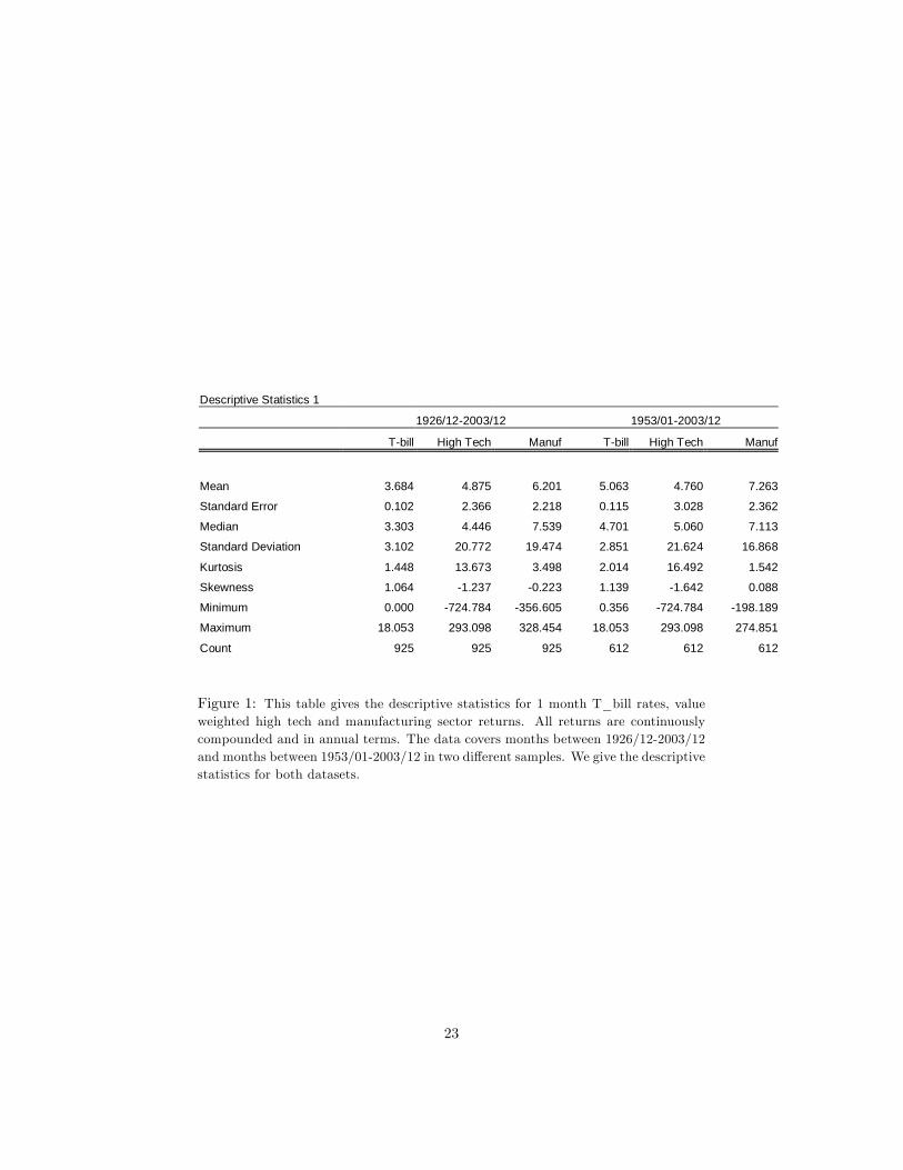
The descriptive statistics on returns are given in �gures 1 and 2 at the endof the paper. These tables show among many things that as sample size getssmaller, the mean returns increase for the Treasury bill and manufacturing sectorand decrease for the high tech sector. The standard deviations decrease for theTreasury bill and manufacturing sector and increase for the high tech sector,with sample size. Kurtosis is largest for high tech, and skewness is negativefor high tech and manufacturing sectors, and positive for Treasury bill. Theminimum is the largest for high tech sector.
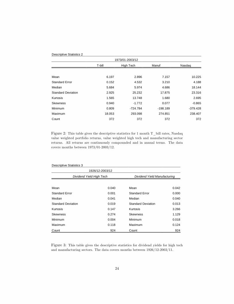
These �gures also show that high tech sector has the lowest mean returnsamong all except for the longest dataset (1926/12-2003/12). In the period1973/01-2003/12, NASDAQ has the highest mean returns. High tech sectoralso has the highest standard deviation among all in all time periods.
We also give the descriptive statistics on dividend yields for both the hightech and manufacturing sectors in �gure 3. The dividends are also obtainedfrom the CRSP database. The dividend yields for each sector is calculated bymultiplying the dividend yield for each individual stock within a sector with itslagged weight in that sector.
3 Methodology
We analyze asset allocation in discrete time for an investor with CRRA utilityover terminal wealth. We consider two assets: Treasury bills and a stock index.The investor uses a Markov switching model to forecast returns. We incorporatethe parameter uncertainty taking a Bayesian approach, where the uncertaintyabout the parameters is summarized by the posterior distribution of the para-meters. We then will compare the case with uncertainty with the case withoutuncertainty where the distribution of returns is constructed conditional on �xedparameter estimates.
6
3.1 Asset Allocation Framework for a Buy-and-Hold In-vestor
Suppose we are writing down the portfolio problem for a buy-and-hold investorwith a horizon of bT months and we�re initially at time T. Suppose further thatwe have two assets: Treasury bills and a stock index. We suppose that thecontinuously compounded monthly return on Treasury bills is a constant rf : Inour numerical framework we set rf equal to 0.000361, which is the return onDecember 2003 (the last month of our sample) of the one month Treasury bill(since this return is unusually small, we also try the average return on one monthT-bill rates over our samples). We model the excess returns on the stock indexusing a Markov switching framework. It takes the form
rt = �st + et; et�N(0; �2st); (1)
�St = �1S1t + �2S2t; (2)
�2St = �21S1t + �
22S2t; (3)
Sjt = 1; if St = j; and Sjt = 0; otherwise; j = 1; 2; (4)
pij = Pr[St = jjSt�1 = i]: (5)
If initial wealth WT = 1 and w is the allocation to the stock index, thenend-of-horizon wealth is given by
We ignore intermediate consumption (the investor is assumed to consumeend of period wealth, WT+bT ):Then, the investor�s preferences over terminal wealth are given by a CRRA
utility function, u(W)=W 1�A
1�A ; and the buy-and-hold investor�s problem is tosolve
7
maxw
ET (f(1� w) exp(rf bT ) + w exp(rf bT + rT+1 + rT+2 + :::::+ rT+bT )g1�A
1�A ):
(7)
We then consider two cases to calculate this expectation, one without pa-rameter uncertainty and one with parameter uncertainty. In the case withoutparameter uncertainty the investor solves
maxw
Zu(WT+bT )p(RT+bT jy;b�)dRT+bT ; (8)
where y is the data observed by the investor up until the start of his invest-ment horizon (y=(r1; r2; r3; ::::rT )0) and RT+bT = rT+1 + rT+2 + ::::: + rT+bT isthe cumulative return. p(RT+bT jy;b�) is the distribution for future stock returnsconditional on a set of parameter estimates, b�; and y. In the case with parameteruncertainty the problem becomes
maxw
Zu(WT+bT )p(RT+bT jy; �)p(�jy)dRT+bT d�; (9)
where p(�jy) is the posterior distribution and p(RT+bT jy; �) is the likelihood.In this paper, we consider a normal likelihood. In words, the last maximizationproblem means that, rather than constructing the distribution of future returnsconditional on �xed parameter estimates, we integrate over the uncertainty inthe parameters captured by the posterior distribution.
We approximate the integral for expected utility by taking a sample (R(i)T+bT )i=Ii=1
from one of the two distributions (distribution of returns conditional on�xed parameter values or predictive distribution obtained by using the posteriordistributions and the likelihood) and then for w=0,0.01,0.02,....,0.99 computing
We then report the value of w that maximizes the above expression.
In the case without parameter uncertainty, we take 10,000 independent draws(indeed 12,000 draws, but we discard the �rst 2000 draws) from the normal dis-tribution with mean and variance equal to the posterior mean and posterior
8
variance. In appendix A we explain in detail how we �nd the posterior distribu-tions. For the case with parameter uncertainty, we use the posterior distributionto obtain the predictive distribution. After we �nd the posterior distributions,sampling from the predictive distribution is equivalent to �rst sampling fromthe posterior distributions and then the likelihood. This is to say that for eachof the 10,000 (�; �2) pairs drawn, we sample once from the normal distribution3 .
3.2 Markov Switching Models and Gibbs Sampling
The basic di¤erence of the Gibbs Sampling approach to inference on Markovswitching models from the classical approach is that in the Bayesian analy-sis, both the parameters of the model and the Markov switching variable,St; t = 1; 2; ::::; T (one doesn�t observe St; just knows that it is an outcomeof an unobserved, discrete-time, discrete-state Markov process), are treated asrandom variables. Therefore, in contrast to the classical approach, inference onfST (= [S1 S2:::::ST ]0) is based on a joint distribution. In the classical approach,inference on Markov switching models consists of �rst estimating the model�sunknown parameters, then making inferences on the unobserved Markov switch-ing variable, fST ; conditional on the parameter estimates. In Bayesian approach,both the parameters of the model and the unobserved Markov switching vari-ables are treated as missing data, and they are generated from appropriateconditional distributions using Gibbs Sampling.
3.3 Gibbs Sampling
The main model we are using in this paper is the Bayesian alternative to theanalysis of the two-state Markov switching mean-variance model of returns(equations 1-5).
The Gibbs Sampling procedure is given by successive iteration of the follow-ing steps:
Step 1 Generate fST ; conditional on e�2; e�; ep;frTStep 2 Generate ep; conditional on fSTStep 3 Generate e�2; conditional on e�;frT ;fSTStep 4 Generate e�; conditional on e�2;frT ;fST3We should note at this point that the reason why we don�t use quadrature methods as
in Ang and Bekaert (2002), instead of the simulations employed here, to evaluate the inte-grals is because the integral in the case without parameter uncertainty is not one-dimensional.Quadrature methods are a good alternative when the integral is one-dimensional like in the�without parameter uncertainty� case or in the special case when bT = 1: Kandel and Stam-baugh (1996), for instance, use quadrature methods; since, then, using a bT = 1; they canobtain a closed-form solution for the predictive distribution.
9
In the case with predictor variables, we include an additional step, Step 5,where we generate e�; conditional on e�2; e�;fST ; where e� represents the coe¢ cientson the predictor variables.4
4 Asset Allocation with Di¤erent Models
4.1 Empirical Results with the Linear Model
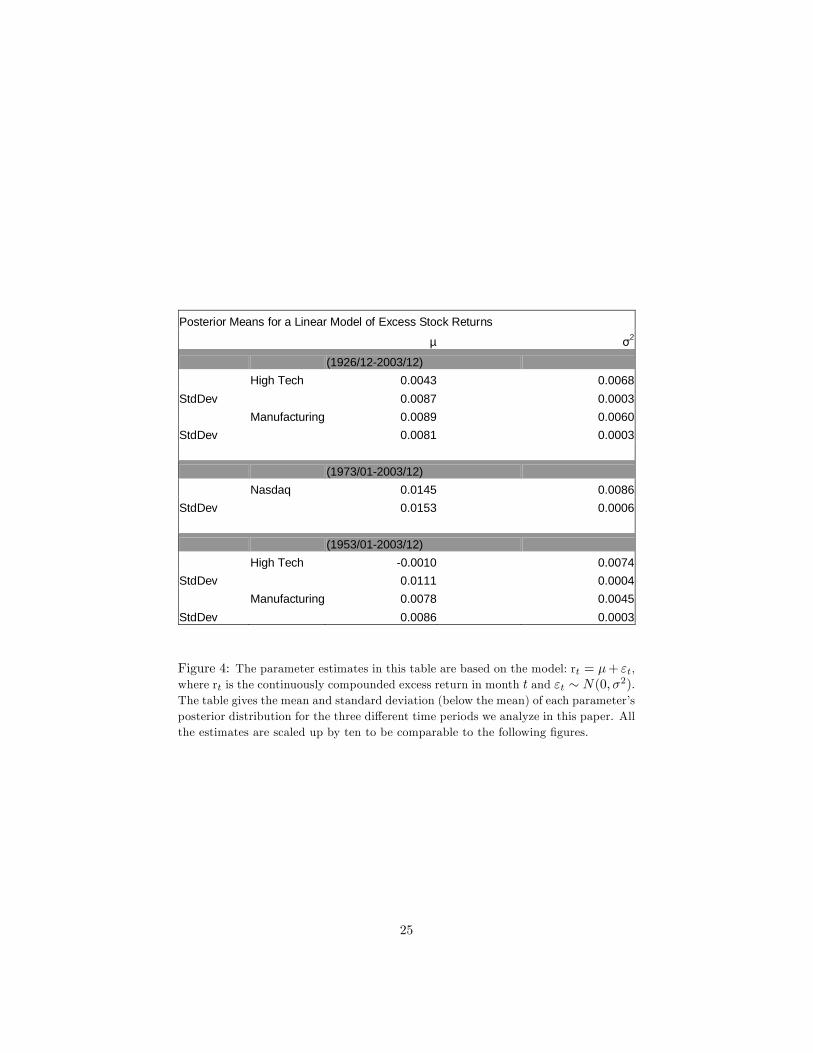
Figure 4 gives the parameter estimates (posterior means) for the linear model(no Markov switching returns and no predictor variables). More explicitly, themodel that we base our results on, in �gure 4, is:
rt = �+ "t; (11)
where rt is the continuously compounded excess return in month t, and"t � N(0; �2): We run this regression for each of the three series (NASDAQ,high tech, manufacturing). One can see from these estimates that high techsector has a lower posterior mean return and a higher posterior standard de-viation than manufacturing sector with both the shorter and longer datasets.NASDAQ, although not directly comparable since its estimates are calculatedwith a di¤erent time period, has a higher posterior mean return and a higherposterior standard deviation than both sectors across all time periods.
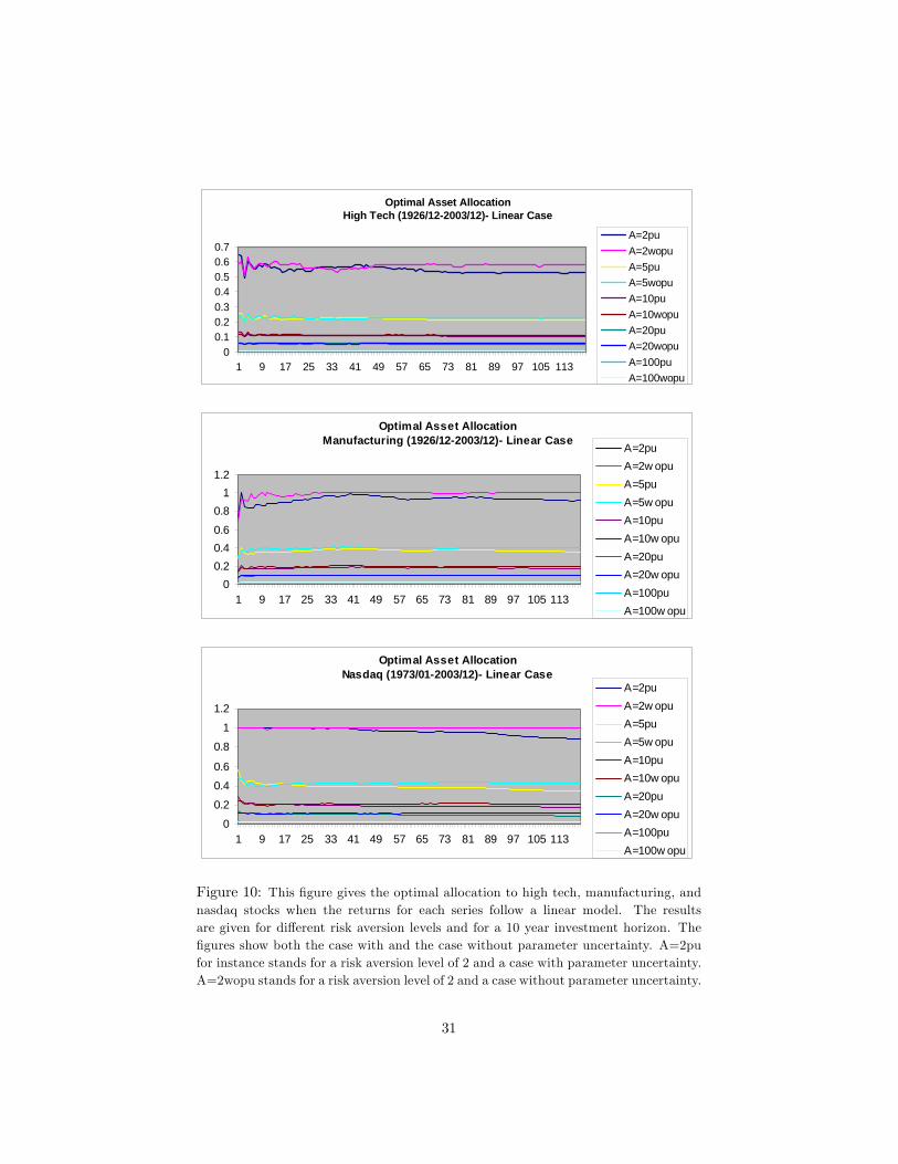
We give the optimal allocations w for the three di¤erent series (NASDAQ,high tech, manufacturing) versus the risk free rate, for a variety of risk aversionlevels A, and with and without parameter uncertainty for the linear model in�gure 10. We give the results for a 10 year investment horizon and utilizing thelonger dataset we have (where the time period is 1926/12-2003/12) in �gure 10.The vertical axis in this �gure represents the optimal weights and the horizontalaxis represents the horizon in months. The results look similar to the resultsin Barberis (2000). The optimal allocation to high tech sector stocks is lowerthan the optimal allocation to NASDAQ and manufacturing sector stocks, andall series exhibit almost �at optimal allocation levels throughout the investmenthorizon of 10 years. These results also con�rm the Samuelson (1969) and Merton(1969) results for a buy-and-hold investor5 .
4Generations of these conditional distributions are explained in further detail in AppendixA, a la Kim and Nelson (1998). Please refer to Kim and Nelson (1998) for more details onthe Gibbs Sampling method.
5Note that Samuelson (1969) and Merton (1969) analyze the setting with i.i.d. returns andoptimal rebalancing, where we analyze the setting with a linear model and a buy-and-holdinvestor.
10
4.2 Empirical Results with the Regime Switching Model
In this section, we run the univariate regressions of returns on the NASDAQ,high tech and manufacturing indices, and �nd the optimal portfolio weightsw when these returns are used in the optimal asset allocation problem versusrisk free rates.
The model for high tech and manufacturing sectors is as follows6 :
rht = �hst + "
ht (12)
rmt = �mst + "
mt (13)
In this model, there�s not an impact of manufacturing sector on high techsector and vice versa. We assume that sectors have �independent�processes inthis model. We run the equations separately, calculate the predictive distribu-tion of returns from the posterior distributions (or posterior means for the casewithout parameter uncertainty) obtained from each run of the Gibbs Samplingprocedure and obtain the optimal asset allocation of each index versus the riskfree asset.
This model follows a similar structure to the model we introduced in equa-tions 1-5, where both the means and variances of the process are regime depen-dent. In the results given in this section, sig_1 refers to the variance in the �rststate, and sig_2 refers to the variance in the second state; whereas mu_1 refersto the mean in the �rst state, and mu_2 refers to the mean in the second state.
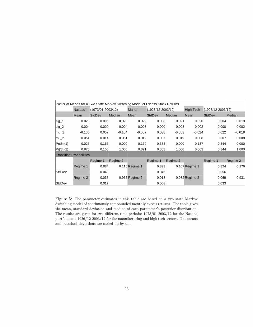
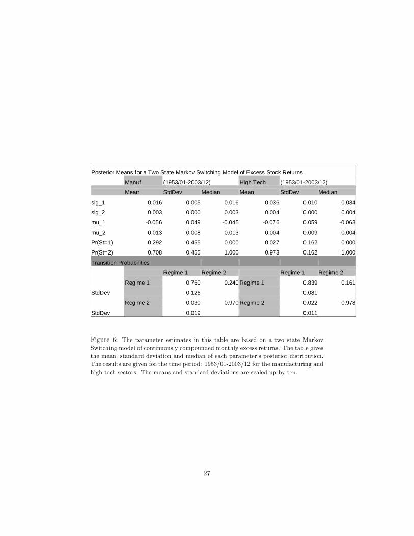
Figures 5-6 report the parameter estimates following a Bayesian Gibbs Sam-pling approach to a two-state Markov switching mean-variance model of excessreturns. Monthly CRSP data for the period 1973/01-2003/12 is utilized for theNASDAQ portfolio and monthly CRSP data for the period 1926/11-2003/12 isutilized for the high tech and manufacturing sector portfolios in Figure 5; andmonthly CRSP data for the period 1953/01-2003/12 is utilized for the high techand manufacturing sector portfolios in Figure 6.
As we can see from �gure 5, the persistence levels of states for the NAS-DAQ portfolio is about 9 and 29 months respectively for states 1 and 2. Formanufacturing and high tech sectors, the persistence levels are about 9, 56 and6, 15 for the �rst and second states with the long dataset. The �rst state forNASDAQ is the state with the higher variance and lower mean excess return
6We also tried to include di¤erent order AR processes in our model, but found no signi�cante¤ect of lags on the process, so we decided to leave the lags out.
11
(indeed negative), which is also the state in which NASDAQ stocks stay less.(The allure of the NASDAQ stocks might be this, that the investors even if theyassume that they�re in the �rst state, knowing that it�s not going to last longmight be overinvesting.) With the long dataset, the manufacturing and hightech sectors also stay less in the �rst state and the �rst state is the state withlower mean excess returns (negative) and higher variances. In comparing (if atall) the NASDAQ index with the high tech sector, one should keep in mind thedi¤erent time periods utilized for the two series.
The persistence levels are 4, 33 and 6, 46 for states 1 and 2, for manufacturingand high tech sectors, respectively, with the short dataset. With the shortdataset, again, for both the manufacturing and high tech sectors, state 1 is thestate with negative mean excess returns and higher variances, and where bothseries stay less.
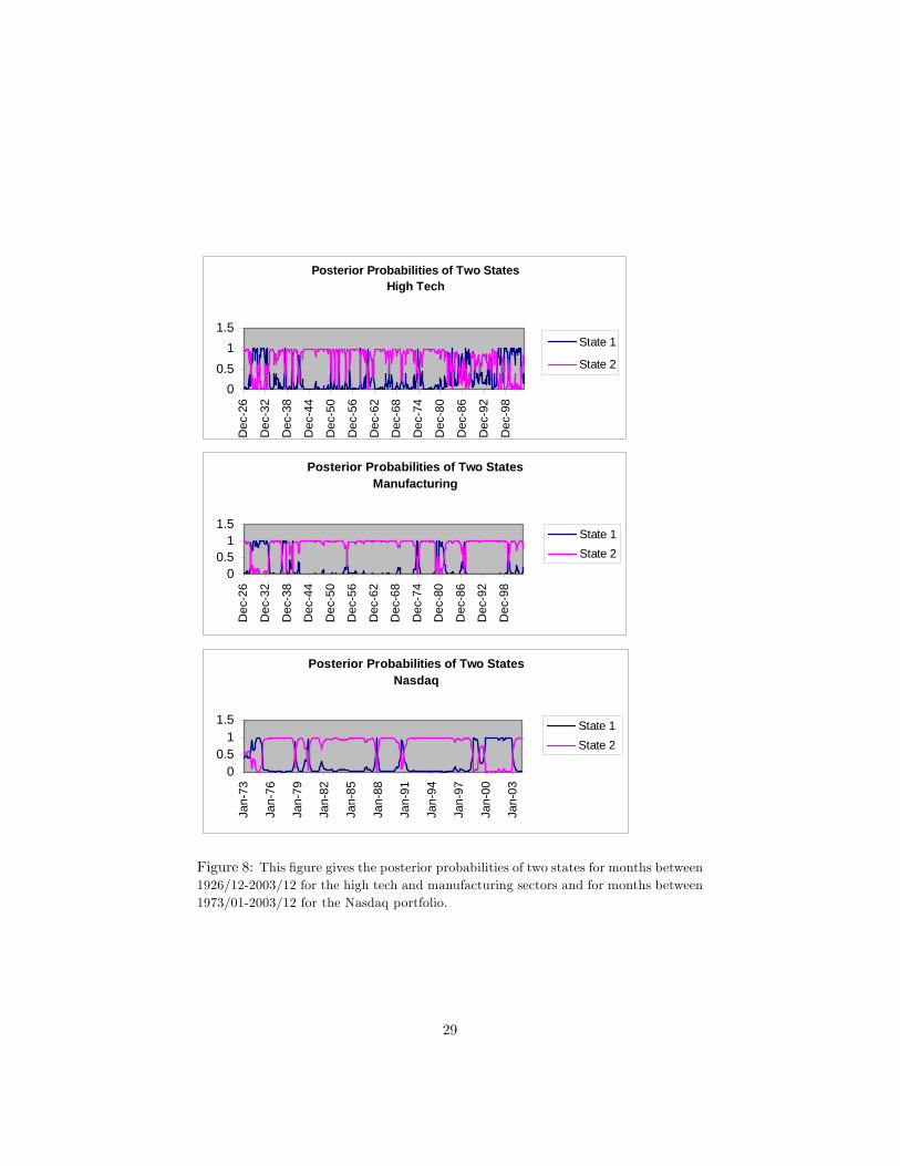
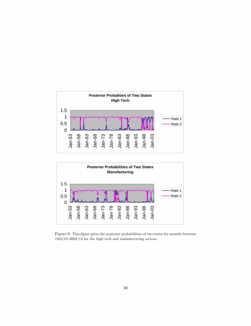
The posterior distributions given in �gures 8 and 9 are calculated by gener-ating 12,000 draws. The �rst 2,000 draws are discarded. These �gures give theposterior probabilities of the two di¤erent states for the three series we use inour paper: NASDAQ portfolio, high tech and manufacturing sector portfolioswith the long and short datasets respectively. It seems like, roughly, the regimesshift around 1929, 1938, 1942, 1960, 1974, 1982, 1996 for the high tech sector;around 1928, 1937, 1974, 1980, 1987, 1999 for the manufacturing sector, withthe longer dataset; and around 1973, 1978, 1980, 1987, 1990, 1998 for NASDAQ.With the shorter dataset, for the high tech sector, the regime shifts seem liketaking place, roughly, around 1958, 1960, 1984, 1987, 1996; and with the shorterdataset, for the manufacturing sector, the regime shifts seem like taking place,roughly, around 1955, 1974, 1980, 1987, 1999.
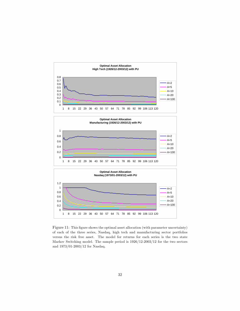
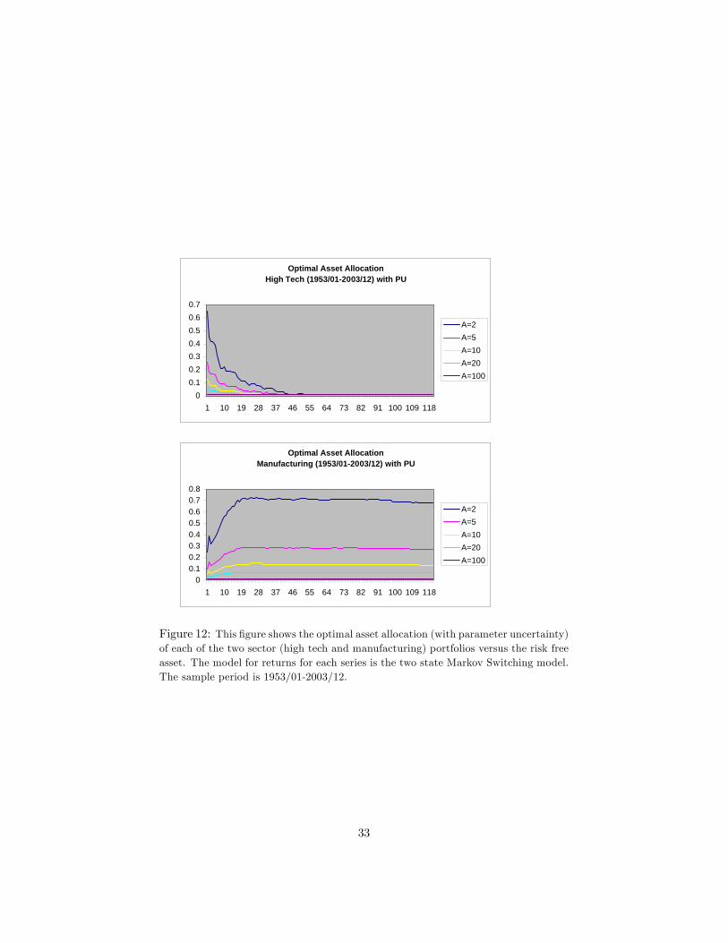
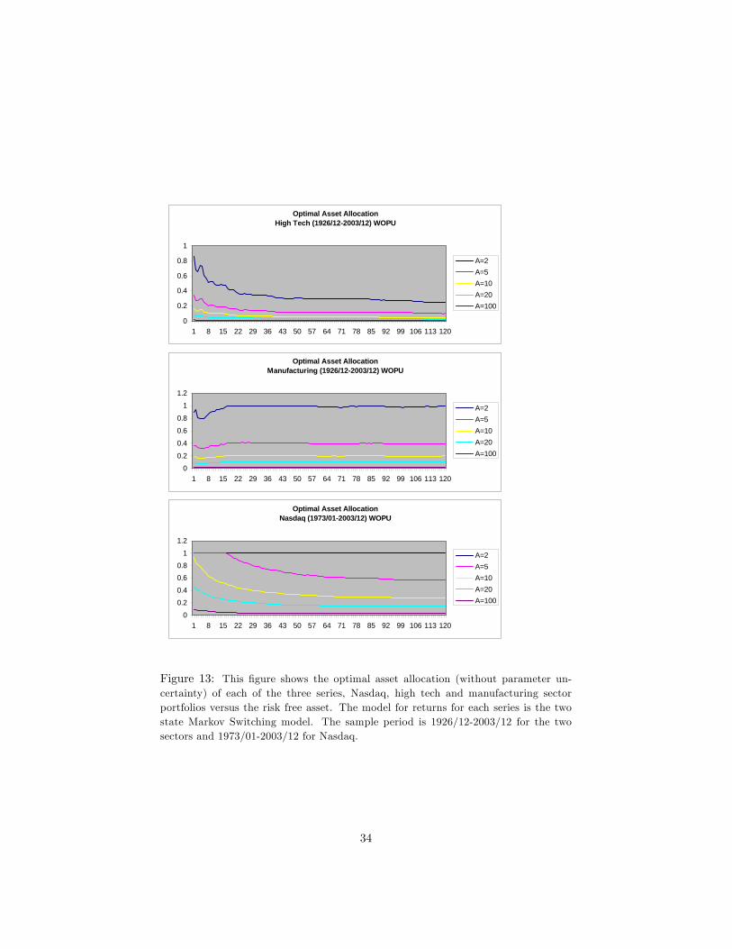
We present the optimal allocations w which maximize the expected utility fora variety of risk aversion levels A, with an investment horizon bT of 10 years andfor di¤erent cases where the investor either ignores or accounts for parameteruncertainty with the two-state Markov switching model in �gures 11-13. In�gures 11-13, as in �gure 10, the vertical axis represents the optimal weightsand the horizontal axis represents the horizon in months. Figures 11-12 give thecase with parameter uncertainty and �gure 13 gives the case without parameteruncertainty. Figure 11 gives the results for the longer sample period (1926/12-2003/12) for the manufacturing and high tech sectors, and �gure 12 gives theresults for the shorter sample period (1953/01-2003/12) for the manufacturingand high tech sectors. Figure 11 also includes the results for NASDAQ for thesample period 1973/01-2003/12. For the case without parameter uncertainty,we do not give the results for the shorter dataset, since these results look similarto the results with the longer dataset.
We �nd out from these �gures that the static buy-and-hold investor allo-cates less to equities as the horizon increases for the NASDAQ and high techseries once parameter uncertainty is taken into account. The reason why the
12
investor allocates less to equities as the horizon increases is because incorporat-ing uncertainty increases the variance of the distribution for cumulative returns,particularly at longer horizons. This makes stocks look riskier to a long-termbuy-and-hold investor reducing their attractiveness.
The e¤ect is smaller for manufacturing with the long dataset (�gure 11), in-deed optimal allocation to manufacturing stays around the same level through-out the whole investment horizon for the di¤erent risk aversion levels. The e¤ectfor manufacturing actually reverses in the short dataset (�gure 12): the staticbuy-and-hold investor allocates more to equities as the horizon increases. Thisbehavior might be due to the state the manufacturing sector is perceived to bein at the time of the forecast.
The more risk-averse the investor is (the higher the A is), the smaller theoptimal allocation to stocks is in all three series, and all �gures. As can beseen in �gure 11, when the parameter uncertainty is taken into account, theinvestor allocates a big portion of his wealth to stocks only if he�s very riskloving for NASDAQ. Otherwise, the optimal allocation decreases in less than ayear. This result is also true for high tech: the optimal allocation with parameteruncertainty for all risk aversion levels decreases in less than a year for high tech.
One last point to note is that, in general, the optimal allocation to NASDAQversus the risk free asset is much higher than the optimal allocation to theindividual sectors versus the risk free asset, but one should be cautious withtaking this result any further since the results for the individual sectors andthe results for NASDAQ are based on di¤erent time periods, as we mentionedearlier.
On the other hand, when the parameter uncertainty is not taken into ac-count (�gure 13), the allocation to stocks is bigger than the allocation to stockswith parameter uncertainty being taken into account (�gure 11). This result istrue for all our series and for all the di¤erent sample periods and risk aversionlevels we utilize, which is expected, since taking into account the parameteruncertainty always makes the stocks look riskier.
In �gures 11-13, when we utilize the sample averages of the risk free rateinstead of the time T (last period) risk free rate, we �nd similar results, so wedo not see the need to exhibit those �ndings.
4.3 Empirical Results with Predictor Variables
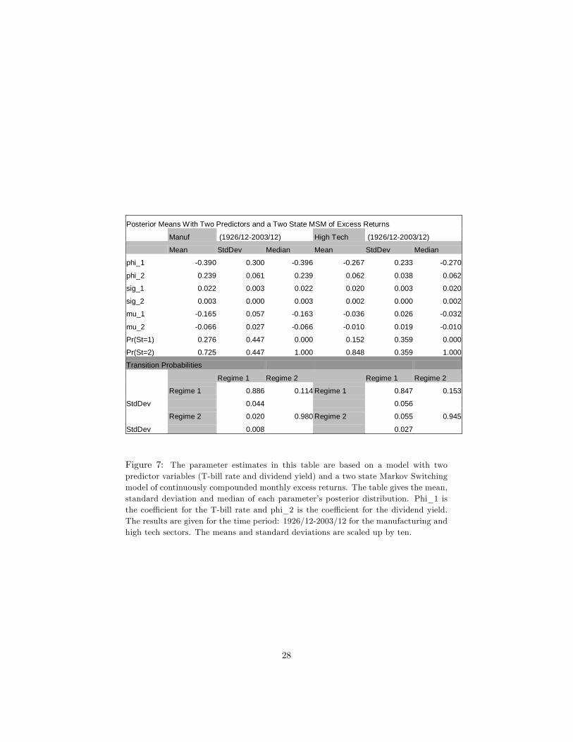
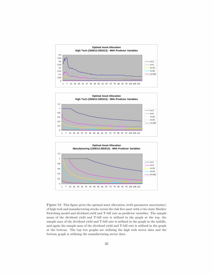
In this section, we give the results for the two-state Markov switching modelwhen we include the dividend yield and T-bill rate as extra predictor variables inthe model. Figure 7 gives the parameter estimates for this model. It shows that
13
the coe¢ cient for the T-bill rate is negative (phi_1) and the coe¢ cient for thedividend yield is positive (phi_2) as one would expect. State 2 is still the statewith higher mean excess returns and lower variances, although the mean excessreturns are negative for both states for both sectors now. The variances remainlower for the second state, and higher for the �rst state. The persistence levelsare about the same as they are before the predictor variables are included in themodel: approximately 9 and 50 months for the manufacturing sector and 7 and18 months for the high tech sector, for the �rst and second states respectively.
The graphs for this model with parameter uncertainty are given in �gure14. The results without parameter uncertainty are similar with weights slightlyhigher than the weights with parameter uncertainty, so we do not see the need toexhibit those results. We only give the results for the longer dataset (1926/12-2003/11 sample period). We utilize di¤erent values for the dividend yield andT-bill rate in �gure 14 to show how the prediction changes when we changethese values. The graph at the top in �gure 14 utilizes the sample mean of thedividend yield for high tech and T-bill rate, which are given in �gures 1 and 3.The graph in the middle gives the results with utilizing the sample maximum ofthe dividend yield for high tech and T-bill rate, which are also given in �gures 1and 3. We do not give the results with utilizing the last period (time T) dividendyield for high tech and T-bill rate since they are unusually small. The graph atthe bottom gives the results with utilizing the sample maximum of the dividendyield for manufacturing and T-bill rate. We do not give the results with utilizingthe last period value and sample mean of the dividend yield for manufacturingand T-bill rate since they are comparatively small, and the optimal allocationto stocks with these values looks really low throughout the whole investmenthorizon.
We can see from �gure 14 that including dividend yield and T-bill rate asextra predictor variables in the two-state Markov switching model, dependingon the initial values of dividend yield and T-bill rate employed, changes themagnitude of the allocation to stocks versus the risk free asset, but it doesn�treduce the riskiness of stocks as the horizon increases. Indeed, the optimalallocation to stocks still decreases as the horizon increases. This in our opinionshows that the predictive power of the dividend yield and T-bill rate at longhorizons is not strong enough to overcome the impact of uncertainty.
4.4 Empirical Results with Two Risky Assets versus theRisk Free Asset
We also calculate the optimal asset allocation of two risky sector indices (hightech and manufacturing portfolios) versus the risk free asset to show the sector-wise optimal asset allocation decision implications of Markov switching returns
14
with parameter uncertainty, hence the reason why we do our analysis on sectorindices.
In this case, we approximate the integral for expected utility by taking a
sample (Rh(i)
T+bT )i=Ii=1 from the predictive distribution of the high tech excess re-
turns and another sample (Rm(i)
T+bT )i=Ii=1 from the predictive distribution of themanufacturing excess returns, which we calculate using the likelihood and pos-terior distributions of returns using the model in section 4.2 (equations 12-13).We then for wh=0,0.01,0.02,....,0.99 and wm=0,0.01,......0.99 (with the conditionthat wh+wm<1) compute:
1
I
IXi=1
f(1� wh � wm) exp(rf bT ) + wh exp(Rh(i)
T+bT ) + wm exp(Rm(i)
T+bT )g1�A1�A : (14)
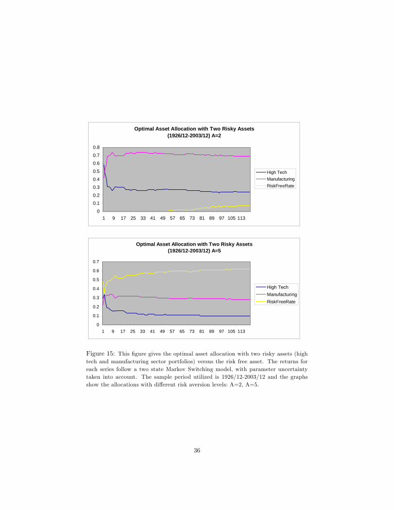
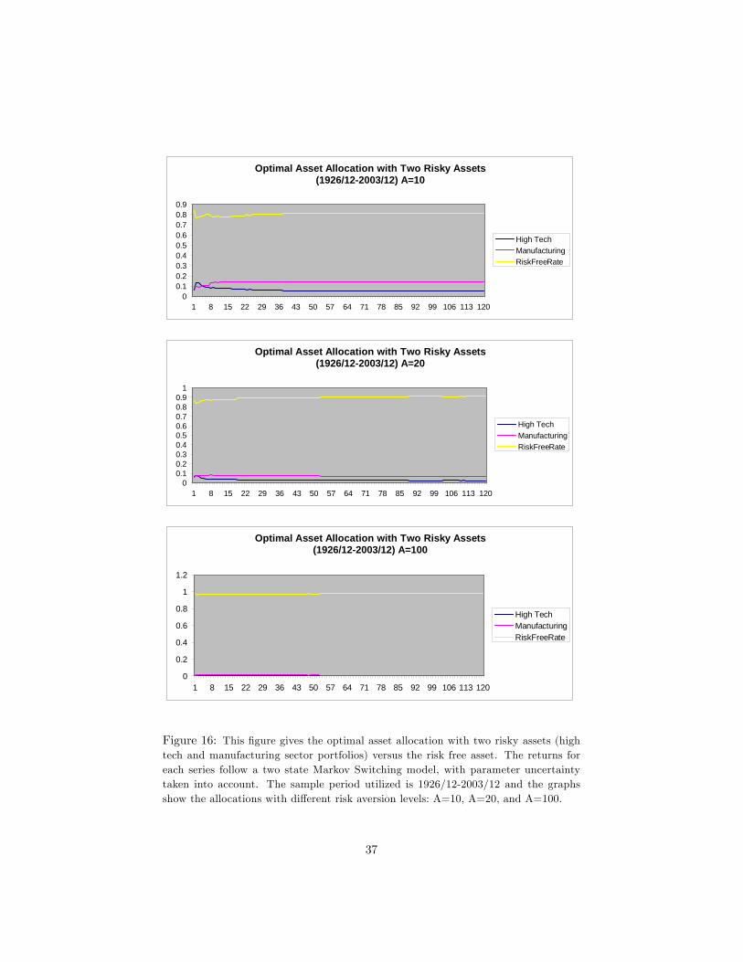
We report the (wh; wm) pairs that maximize the above expression in �gures15 and 16. Figure 15 is with a ten year horizon, with the longer dataset (1926/12-2003/12), for risk aversion levels of 2 and 5, and �gure 16 is with a ten yearhorizon, with the longer dataset, for risk aversion levels of 10, 20 and 100.
We conclude from �gures 15 and 16 that, as would be expected, the optimalallocation to risk free asset increases with risk aversion level and with time. Wealso conclude that the optimal asset allocation to high tech stocks in the presenceof manufacturing stocks (besides the risk free asset) decreases more severely thanthe case without the manufacturing stocks being present. The allocation tomanufacturing stocks with low risk aversion levels (A=2 for instance) actuallyincreases as the horizon increases. The optimal allocation to stocks (eithersector) is minimal with very high risk aversion levels (A=10,20,100 for instance).
4.5 Estimation with a Multivariate (Two Sector) Model
An extension of the analysis to include a regime switching vector auto regression(RSVAR) to capture a variety of interactions between the two sectors will be asfollows:
�rhtrmt
�=
��hst�mst
�+
��h1 ::::�
h3
�m3 ::::�m1
� �rht�1rmt�1
�+
�"ht"mt
�(15)
where we assume "ht ~ N(0; �2h
st ) and "mt ~ N(0; �2
m
st ):
15
This model focuses on two sectors, and follows an AR(1) process, but sincewe doubt that the AR coe¢ cients will be signi�cant, the second right hand sideterm can be ignored in the estimation practices after running initial regressions.In this model, both the means and variances are still regime dependent, and thecovariance matrices reveal the correlations between the two sector returns.
One can estimate the model with and without assuming parameter uncer-tainty, with and without assuming perfect correlation across states in the twosectors. In the case of only two sectors, there�s not much necessity to assumeperfect correlation (since the number of total states in the RSVAR model, ifeach sector return follows a two-state regime switching model in the univari-ate regressions, will only be four, 22), but if we decide to include more thantwo sectors (e.g., n), since we will have to estimate a 2n transition probabilitymatrix, and this is hardly tractable, it�ll be quite convenient to assume perfectcorrelation across the states of the n sectors, although this will put a doubt onthe reliability of the estimation results.
4.6 More Robustness Checks
Besides using di¤erent sample periods, risk aversion levels, and series; we alsoemployed di¤erent initial values and priors for the series we investigate and randi¤erent number of simulations to see if 10,000 draws was giving us accurateenough answers or not, and we saw that changing the initial values, priors orthe number of simulations didn�t change our results signi�cantly.
5 Conclusion
Some investors might ignore that returns follow a Markov switching process,others might instead ignore the uncertainty regarding the parameters of thisMarkov switching process. We show in this paper that ignoring the parame-ter uncertainty leads the investor overallocate to stocks, when returns follow aMarkov switching process.
We also �nd in this paper that the static buy-and-hold investor allocatesless to equities as the horizon increases for two (NASDAQ, high tech) out of thethree series we analyze (NASDAQ, high tech, manufacturing) once the nonlin-earity in the returns process is incorporated. For the shorter dataset we employ(using postwar data), the optimal allocation to manufacturing sector versus therisk free asset actually increases as the horizon increases. This brings us to theconclusion that some investment advisors�suggestion that long horizon investorsshould allocate more agressively to equities maybe too hasty and one should also
16
consider the type of stocks one invests in and take into account parameter un-certainty and the possible regime switches as well. Indeed taking into accountthe observation that di¤erent series behave di¤erently as the horizon increasesmight actually help with the portfolio diversi�cation decisions. We also shouldnote that this result, that is contrary to Barberis (2000), which says that oneshould allocate less to equities with time, is not unique in the literature. Mas-simo and Timmermann (2005) and Pettenuzzo and Timmermann (2004) also�nd similar results but as we noted earlier, in di¤erent scenarios, and they donot consider the behavior of di¤erent series (sectors) and the impact this mighthave on optimal stock allocation.
In this paper, we also look at the additional predictive power of the dividendyield and T-bill rate in the presence of a two-state Markov switching model, andconclude that the predictive power of these two predictor variables is not strongenough to adverse the e¤ect of parameter uncertainty in the long run, unlikewhat Barberis (2000) suggests.
We also believe that results to an optimal asset allocation problem, as Bawa,Brown, and Klein (1979) suggest, are sensitive to the sample size used in theestimations, since parameter estimation uncertainty is a bigger problem withshorter datasets.
We also think that the uncertainty underlying the current state any series isin is crucial to the optimal asset allocation decision (that�s why we use GibbsSampling methods, and take the current state as unknown). We believe that,incorrectly assuming the current state to be in a certain state (either state 1 or2) would have signi�cant costs, and taking into account the uncertainty aboutthe true state of the series actually reduces these costs.
17
6 Appendix A
6.1 Generating fST ; conditional on e�2; e�; ep; e�; erTThis refers to simulating St; t = 1; 2; :::; T; as a block from the following jointconditional distribution: g(fST j e�2; e�; ep; e�;frT ): To do this, �rst consider thederivation of the joint conditional density: g(fST jfrT ). It�s easy to show that
g(fST jfrT ) = g(ST jfrT )T�1Qt=1g(StjSt+1;frT ); using the Markov property of St that
conditional on St+1; for example St+2;:::::::; ST; and rt+1; ::::rT contain no in-formation beyond that in St+1: To derive the terms in the last equality, thefollowing steps can be employed. First, run Hamilton�s (1989) basic �lter toget g(StjfrT ); t = 1; 2; ::::T; and save them. The last iteration would provide usg(ST jfrT ): In the second step to generate g(StjSt+1;frT ); for t = 1; ::::; T �2; T �1; we make use of the following result: g(StjSt+1;frT ) _ g(St+1jSt)g(StjfrT ):Usingthis last equation generating St is the same as �rst calculating Pr[St = 1jSt+1;frT ] =g(St+1jSt=1)g(St=1jfrT )2P
j=1
g(St+1jSt=j)g(St=jjfrT ) ; then generating a random number from the uniform
distribution. If the generated number is less than or equal to Pr[St = 1jSt+1;frT ]; weset St = 1: Otherwise, we set St = 2:
6.2 Generating transition probabilities conditional on fSTWe will use beta distributions as conjugate priors for the transition probabilities.Then it can be shown that the posterior distributions of pii are given by piijfST �beta(uii + nii;
_uii +
_nii); i = 1; 2; where uii and uii are known from the prior
distributions (pii � beta(uii;_uii) a priori). nij ; i; j = 1; 2 is de�ned as the
total number of transitions from state St�1 = i to St = j; t = 2; 3; ::::T:_nij is
de�ned as the number of transitions from state St�1 = i to St 6= j: Once thepii are generated, generating pij is straightforward: pij =
_pij � (1� pii); where
pij = Pr[St = jjSt�1 = i; St 6= i]; for i 6= j:
6.3 Generating e�2; conditional on e�; e�; erT v; ST
To generate �2j ; j = 1; 2; we can rede�ne �2st as follows: �
2st = �
21(1+S2th2):Then
we can generate �21 conditional on h2; by �rst dividing et byp(1 + S2th2) =
U; and then choosing an inverse gamma distribution as the prior for �21 (IG(v12 ;
�12 )):
Then the posterior for �21 is given by �21jfrT ;fST ; h2 � IG(v1+T2 ;
�1+TPt=1
(e�t )2
2 );
18
where v1 and �1 are known hyperparameters of the prior distribution, ande�t is et divided by U de�ned above. Then we generate
_
h2 = 1+ h2; conditionalon �21 to �nd �
22:
6.4 Generating e�; conditional on e�2; e�; erT vST
It is straightforward to derive the posterior distribution of � = [�1 �2]0; given an
appropriate prior distribution such as the normal: �je�2; e� � N(a0; A0); where a0 andA0 are known hyperparameters of the prior distribution. Then the poste-rior is: �je�2; e�;frT ;fST � N(a1; A1) where a1 = (A�10 + S�0T S
�T )�1(A�10 a0 +
S�0T r�T ); A1 = (A
�10 + S�0T S
�T )�1; where S�it = Sit; and S
�T is the matrix form of
S�it; each element divided by �St to correct for heteroskedasticity; r�T is the ma-
trix form of r�t ; each element divided by �St to correct for heteroskedasticity, where r�t =
rt:
6.5 Generating e�; conditional on e�2; e�f; rT v; ST
If we let rt = �St +X�St + v; and then divide it by �st ; then given the a prioridistribution for e� as e�je�2; e� � N(b0; B0); where b0 and B0 are known hyperpara-meters of the prior distribution, the posterior can be written as e�je�2; e�;frT ;fST �N(b1; B1); where b1 = (B
�10 +X 0X)�1(B�10 b0 +X
0r); B1 = (B�10 +X 0X)�1:
6.6 Prior Elicitation
We make use of the following prior hyperparameters.
For the hyperparameters of the prior for the transition probabilities (wherethe prior is a beta distribution) we use:
pii � beta(uii;_uii)) uii = 0:1;
_uii = 0:1:
For the hyperparameters of the prior for the variances (where the prior is aninverted gamma distribution) we use:
�2i � IG(vi2 ;�i2 )) vi = 0; �i = 0:
For the hyperparameters of the prior for the means (where the prior is anormal distribution) we use:
19
� � N(a0; A0)) a0 = 0:04; A0 = 0j0:1:
For the hyperparameters of the prior for the coe¢ cients (where the prior isa normal distribution) we use:
� � N(b0; B0)) b0 = 0; B0 = 0j0:
20
7 References
Ang, A., and G. Bekaert, 2002, "International Asset Allocation with RegimeShifts," Review of Financial Studies, 15, 4, 1137-1187.
Barberis, Nicholas, 2000, �Investing for the Long Run when Returns arePredictable,�Journal of Finance, Vol. LV, No.1.
Bawa, V., S. Brown, and R. Klein, 1979, "Estimation Risk and OptimalPortfolio Choice" (North Holland, Amsterdam).
Beller, K., J. Kling, and M. Levinson, 1998, "Are Industry Stock ReturnsPredictable?," Financial Analysts Journal, Vol. 54, No. 5, Sep/Oct, 42-57.
Bodie, Zvi, 1995, "On the Risk of Stocks in the Long Run," Financial Ana-lysts Journal 51, 18-22.
Capaul, Carlo, 1999, "Asset Pricing Anomalies in Global Industry Indexes,"Financial Analysts Journal, Vol. 55, No. 4, Jul/Aug, 17-37.
Cavaglia, S., and V. Moroz, 2002, "Cross-Industry, Cross-Country Alloca-tion," Financial Analysts Journal, Vol. 58, Issue 6, Nov/Dec, p.78.
Fama, E.F., and K.R. French, 1988a, "Permanent and Temporary Compo-nents of Stock Prices," Journal of Political Economy, Vol. 96, No. 2, April,246-73.
Ferson, W.E., and C.R. Harvey, 1991, " The Variation of Economic RiskPremiums," Journal of Political Economy, Vol. 99, No. 2, April, 385-415.
Frost, P., and J. Savarino, 1986, "An empirical Bayes Approach to E¢ cientPortfolio Selection," Journal of Financial and Qualitative Analysis 21, 293-305.
Hamilton, James, �A New Approach to the Economic Analysis of Non-Stationary Time Series and The Business Cycle,�Econometrica, March 1989,57, 357-84.
Hamilton, J.D., and R. Susmel, 1994, "Autoregressive Conditional Het-eroskedasticity and Changes in Regime," Journal of Econometrics 64, 307-333.
Jobson, J.D., and R. Korkie, 1980, "Estimation for Markowitz E¢ cient Port-folios," Journal of the American Statistical Association 75, 544-554.
Jorion, Phillipe, 1985, "International Portfolio Diversi�cation with Estima-tion Risk," Journal of Business 58, 259-278.
21
Kandel, S., and R. Stambaugh, 1996, "On the Predictability of Stock Re-turns: An Asset Allocation Perspective," Journal of Finance 51, 385-424.
Kim, C.J., and C. R. Nelson, "State-Space Models with Regime Switching:Classical and Gibbs-sampling Approaches with Applications," 1998, MIT Press.
Lo, A., and A.C. MacKinlay, 1996, "Maximizing Predictability in the Stockand Bond Markets," NBER Working Paper, #5027, February 1995.
Massimo G., and A. Timmermann, 2005, "Strategic Asset Allocation andConsumption Decisions Under Multivariate Regime Switching," Working Papers2005-002, Federal Reserve Bank of St. Louis.
Merton, Robert, 1969, "Lifetime Portfolio Selection: The Continous-TimeCase," Review of Economics and Statistics 51, 247-257.
Moskowitz, T.J., and M. Grinblatt, 1999, "Do Industries Explain Momen-tum?," Journal of Finance, Vol. 54, No. 4, August, 1249-90.
Perez-Quiros, G., and A. Timmermann, 2001, "Business Cycle Asymme-tries in Stock Returns : Evidence from Higher Order Moments and ConditionalDensities," Working Paper Series 58, European Central Bank.
Pettenuzzo, D., and A. Timmermann, �Optimal Asset Allocation underStructural Breaks,�job market paper.
Samuelson, Paul, 1969, "Lifetime Portfolio Selection by Dynamic StochasticProgramming," Review of Economics and Statistics 51, 239-246.
Samuelson, Paul, 1994, "The Long-Term Case for Equities," Journal of Port-folio Management, Fall, 15-24.
Schwert, G. William, 1989, �Business Cycles, Financial Crises, and StockVolatility,� Carnegie-Rochester Conference Series on Public Policy, Vol. 31,83-126.
Siegel, Jeremy, 1994, "Stocks for the Long Run" (Richard D. Irwin, BurrRidge, Ill.).
Sorenson, E., and T. Burke, 1986, "Portfolio Returns from Active IndustryGroup Rotation," Financial Analysts Journal, Vol. 46, No. 5, Sept/Oct, 43-50.
Turner, C. M., R. Startz, and C. R. Nelson, 1989, �A Markov Model of Het-eroskedasticity, Risk, and Learning in the Stock Market,�Journal of FinancialEconomics, Vol. 25, 3-22.
Schaller, H. and S. Van Norden, 1997, "Regime Switching in Stock MarketReturns," Applied Financial Economics, Taylor and Francis Journals, vol. 7(2),pages 177-91.
22
Descriptive Statistics 1
1926/12-2003/12 1953/01-2003/12
T-bill High Tech Manuf T-bill High Tech Manuf
Mean 3.684 4.875 6.201 5.063 4.760 7.263
Standard Error 0.102 2.366 2.218 0.115 3.028 2.362
Median 3.303 4.446 7.539 4.701 5.060 7.113
Standard Deviation 3.102 20.772 19.474 2.851 21.624 16.868
Maximum 18.053 293.098 328.454 18.053 293.098 274.851
Count 925 925 925 612 612 612
Figure 1: This table gives the descriptive statistics for 1 month T_bill rates, valueweighted high tech and manufacturing sector returns. All returns are continuouslycompounded and in annual terms. The data covers months between 1926/12-2003/12and months between 1953/01-2003/12 in two di¤erent samples. We give the descriptivestatistics for both datasets.
23
Descriptive Statistics 2
1973/01-2003/12
T-bill High Tech Manuf Nasdaq
Mean 6.197 2.896 7.157 10.225
Standard Error 0.152 4.532 3.210 4.188
Median 5.684 5.974 4.686 18.144
Standard Deviation 2.925 25.232 17.875 23.316
Kurtosis 1.565 13.748 1.680 2.695
Skewness 0.940 -1.772 0.077 -0.865
Minimum 0.809 -724.784 -198.189 -379.428
Maximum 18.053 293.098 274.851 238.407
Count 372 372 372 372
Figure 2: This table gives the descriptive statistics for 1 month T_bill rates, Nasdaqvalue weighted portfolio returns, value weighted high tech and manufacturing sectorreturns. All returns are continuously compounded and in annual terms. The datacovers months between 1973/01-2003/12.
Descriptive Statistics 3
1926/12-2003/12
Dividend Yield High Tech Dividend Yield Manufacturing
Mean 0.040 Mean 0.042
Standard Error 0.001 Standard Error 0.000
Median 0.041 Median 0.040
Standard Deviation 0.019 Standard Deviation 0.013
Kurtosis 0.147 Kurtosis 3.266
Skewness 0.274 Skewness 1.129
Minimum 0.004 Minimum 0.018
Maximum 0.118 Maximum 0.124
Count 924 Count 924
Figure 3: This table gives the descriptive statistics for dividend yields for high techand manufacturing sectors. The data covers months between 1926/12-2003/11.
24
Posterior Means for a Linear Model of Excess Stock Returns
µ 2
(1926/12-2003/12)High Tech 0.0043 0.0068
StdDev 0.0087 0.0003Manufacturing 0.0089 0.0060
StdDev 0.0081 0.0003
(1973/01-2003/12)Nasdaq 0.0145 0.0086
StdDev 0.0153 0.0006
(1953/01-2003/12)High Tech -0.0010 0.0074
StdDev 0.0111 0.0004Manufacturing 0.0078 0.0045
StdDev 0.0086 0.0003
Figure 4: The parameter estimates in this table are based on the model: rt = �+ "t,where rt is the continuously compounded excess return in month t and "t � N(0; �2).The table gives the mean and standard deviation (below the mean) of each parameter�sposterior distribution for the three di¤erent time periods we analyze in this paper. Allthe estimates are scaled up by ten to be comparable to the following �gures.
25
Posterior Means for a Two State Markov Switching Model of Excess Stock Returns
Nasdaq (1973/01-2003/12) Manuf (1926/12-2003/12) High Tech (1926/12-2003/12)
Mean StdDev Median Mean StdDev Median Mean StdDev Median
Figure 5: The parameter estimates in this table are based on a two state MarkovSwitching model of continuously compounded monthly excess returns. The table givesthe mean, standard deviation and median of each parameter�s posterior distribution.The results are given for two di¤erent time periods: 1973/01-2003/12 for the Nasdaqportfolio and 1926/12-2003/12 for the manufacturing and high tech sectors. The meansand standard deviations are scaled up by ten.
26
Posterior Means for a Two State Markov Switching Model of Excess Stock Returns
Manuf (1953/01-2003/12) High Tech (1953/01-2003/12)
Mean StdDev Median Mean StdDev Median
sig_1 0.016 0.005 0.016 0.036 0.010 0.034
sig_2 0.003 0.000 0.003 0.004 0.000 0.004
mu_1 -0.056 0.049 -0.045 -0.076 0.059 -0.063
mu_2 0.013 0.008 0.013 0.004 0.009 0.004
Pr(St=1) 0.292 0.455 0.000 0.027 0.162 0.000
Pr(St=2) 0.708 0.455 1.000 0.973 0.162 1.000
Transition Probabilities
Regime 1 Regime 2 Regime 1 Regime 2
Regime 1 0.760 0.240 Regime 1 0.839 0.161
StdDev 0.126 0.081
Regime 2 0.030 0.970 Regime 2 0.022 0.978
StdDev 0.019 0.011
Figure 6: The parameter estimates in this table are based on a two state MarkovSwitching model of continuously compounded monthly excess returns. The table givesthe mean, standard deviation and median of each parameter�s posterior distribution.The results are given for the time period: 1953/01-2003/12 for the manufacturing andhigh tech sectors. The means and standard deviations are scaled up by ten.
27
Posterior Means With Two Predictors and a Two State MSM of Excess Returns
Manuf (1926/12-2003/12) High Tech (1926/12-2003/12)
Mean StdDev Median Mean StdDev Median
phi_1 -0.390 0.300 -0.396 -0.267 0.233 -0.270
phi_2 0.239 0.061 0.239 0.062 0.038 0.062
sig_1 0.022 0.003 0.022 0.020 0.003 0.020
sig_2 0.003 0.000 0.003 0.002 0.000 0.002
mu_1 -0.165 0.057 -0.163 -0.036 0.026 -0.032
mu_2 -0.066 0.027 -0.066 -0.010 0.019 -0.010
Pr(St=1) 0.276 0.447 0.000 0.152 0.359 0.000
Pr(St=2) 0.725 0.447 1.000 0.848 0.359 1.000
Transition Probabilities
Regime 1 Regime 2 Regime 1 Regime 2
Regime 1 0.886 0.114 Regime 1 0.847 0.153
StdDev 0.044 0.056
Regime 2 0.020 0.980 Regime 2 0.055 0.945
StdDev 0.008 0.027
Figure 7: The parameter estimates in this table are based on a model with twopredictor variables (T-bill rate and dividend yield) and a two state Markov Switchingmodel of continuously compounded monthly excess returns. The table gives the mean,standard deviation and median of each parameter�s posterior distribution. Phi_1 isthe coe¢ cient for the T-bill rate and phi_2 is the coe¢ cient for the dividend yield.The results are given for the time period: 1926/12-2003/12 for the manufacturing andhigh tech sectors. The means and standard deviations are scaled up by ten.
28
Posterior Probabilities of Two StatesHigh Tech
00.5
11.5
Dec
-26
Dec
-32
Dec
-38
Dec
-44
Dec
-50
Dec
-56
Dec
-62
Dec
-68
Dec
-74
Dec
-80
Dec
-86
Dec
-92
Dec
-98
State 1
State 2
Posterior Probabilities of Two StatesManufacturing
00.5
11.5
Dec
-26
Dec
-32
Dec
-38
Dec
-44
Dec
-50
Dec
-56
Dec
-62
Dec
-68
Dec
-74
Dec
-80
Dec
-86
Dec
-92
Dec
-98
State 1State 2
Posterior Probabilities of Two StatesNasdaq
00.5
11.5
Jan-
73
Jan-
76
Jan-
79
Jan-
82
Jan-
85
Jan-
88
Jan-
91
Jan-
94
Jan-
97
Jan-
00
Jan-
03
State 1State 2
Figure 8: This �gure gives the posterior probabilities of two states for months between1926/12-2003/12 for the high tech and manufacturing sectors and for months between1973/01-2003/12 for the Nasdaq portfolio.
29
Posterior Probalities of Two StatesHigh Tech
00.5
11.5
Jan-
53
Jan-
58
Jan-
63
Jan-
68
Jan-
73
Jan-
78
Jan-
83
Jan-
88
Jan-
93
Jan-
98
Jan-
03
State 1State 2
Posterior Probabilities of Two StatesManufacturing
00.5
11.5
Jan-
53
Jan-
58
Jan-
63
Jan-
68
Jan-
73
Jan-
78
Jan-
83
Jan-
88
Jan-
93
Jan-
98
Jan-
03
State 1State 2
Figure 9: This �gure gives the posterior probabilities of two states for months between1953/01-2003/12 for the high tech and manufacturing sectors.
30
Optimal Asset AllocationHigh Tech (1926/12-2003/12)- Linear Case
Figure 10: This �gure gives the optimal allocation to high tech, manufacturing, andnasdaq stocks when the returns for each series follow a linear model. The resultsare given for di¤erent risk aversion levels and for a 10 year investment horizon. The�gures show both the case with and the case without parameter uncertainty. A=2pufor instance stands for a risk aversion level of 2 and a case with parameter uncertainty.A=2wopu stands for a risk aversion level of 2 and a case without parameter uncertainty.
31
Optimal Asset AllocationHigh Tech (1926/12-2003/12) with PU
Figure 11: This �gure shows the optimal asset allocation (with parameter uncertainty)of each of the three series, Nasdaq, high tech and manufacturing sector portfoliosversus the risk free asset. The model for returns for each series is the two stateMarkov Switching model. The sample period is 1926/12-2003/12 for the two sectorsand 1973/01-2003/12 for Nasdaq.
32
Optimal Asset AllocationHigh Tech (1953/01-2003/12) with PU
00.10.20.30.40.50.60.7
1 10 19 28 37 46 55 64 73 82 91 100 109 118
A=2A=5A=10A=20A=100
Optimal Asset AllocationManufacturing (1953/01-2003/12) with PU
00.10.20.30.40.50.60.70.8
1 10 19 28 37 46 55 64 73 82 91 100 109 118
A=2A=5A=10A=20A=100
Figure 12: This �gure shows the optimal asset allocation (with parameter uncertainty)of each of the two sector (high tech and manufacturing) portfolios versus the risk freeasset. The model for returns for each series is the two state Markov Switching model.The sample period is 1953/01-2003/12.
Figure 13: This �gure shows the optimal asset allocation (without parameter un-certainty) of each of the three series, Nasdaq, high tech and manufacturing sectorportfolios versus the risk free asset. The model for returns for each series is the twostate Markov Switching model. The sample period is 1926/12-2003/12 for the twosectors and 1973/01-2003/12 for Nasdaq.
34
Optimal Asset AllocationHigh Tech (1926/12-2003/12) - With Predictor Variables
Figure 14: This �gure gives the optimal asset allocation (with parameter uncertainty)of high tech and manufacturing stocks versus the risk free asset with a two state MarkovSwitching model and dividend yield and T-bill rate as predictor variables. The samplemean of the dividend yield and T-bill rate is utilized in the graph at the top, thesample max of the dividend yield and T-bill rate is utilized in the graph in the middle,and again the sample max of the dividend yield and T-bill rate is utilized in the graphat the bottom. The top two graphs are utilizing the high tech sector data and thebottom graph is utilizing the manufacturing sector data.
35
Optimal Asset Allocation with Two Risky Assets(1926/12-2003/12) A=2
0
0.1
0.2
0.3
0.4
0.5
0.6
0.7
0.8
1 9 17 25 33 41 49 57 65 73 81 89 97 105 113
High TechManufacturingRiskFreeRate
Optimal Asset Allocation with Two Risky Assets(1926/12-2003/12) A=5
0
0.1
0.2
0.3
0.4
0.5
0.6
0.7
1 9 17 25 33 41 49 57 65 73 81 89 97 105 113
High TechManufacturingRiskFreeRate
Figure 15: This �gure gives the optimal asset allocation with two risky assets (hightech and manufacturing sector portfolios) versus the risk free asset. The returns foreach series follow a two state Markov Switching model, with parameter uncertaintytaken into account. The sample period utilized is 1926/12-2003/12 and the graphsshow the allocations with di¤erent risk aversion levels: A=2, A=5.
36
Optimal Asset Allocation with Two Risky Assets(1926/12-2003/12) A=10
Figure 16: This �gure gives the optimal asset allocation with two risky assets (hightech and manufacturing sector portfolios) versus the risk free asset. The returns foreach series follow a two state Markov Switching model, with parameter uncertaintytaken into account. The sample period utilized is 1926/12-2003/12 and the graphsshow the allocations with di¤erent risk aversion levels: A=10, A=20, and A=100.