American Finance Association -...

American Finance Association

Data-Snooping, Technical Trading Rule Performance, and the BootstrapAuthor(s): Ryan Sullivan, Allan Timmermann, Halbert WhiteSource: The Journal of Finance, Vol. 54, No. 5 (Oct., 1999), pp. 1647-1691Published by: Blackwell Publishing for the American Finance AssociationStable URL: http://www.jstor.org/stable/222500 .Accessed: 09/05/2011 05:39

Your use of the JSTOR archive indicates your acceptance of JSTOR's Terms and Conditions of Use, available at .http://www.jstor.org/page/info/about/policies/terms.jsp. JSTOR's Terms and Conditions of Use provides, in part, that unlessyou have obtained prior permission, you may not download an entire issue of a journal or multiple copies of articles, and youmay use content in the JSTOR archive only for your personal, non-commercial use.

Please contact the publisher regarding any further use of this work. Publisher contact information may be obtained at .http://www.jstor.org/action/showPublisher?publisherCode=black. .

Each copy of any part of a JSTOR transmission must contain the same copyright notice that appears on the screen or printedpage of such transmission.

JSTOR is a not-for-profit service that helps scholars, researchers, and students discover, use, and build upon a wide range ofcontent in a trusted digital archive. We use information technology and tools to increase productivity and facilitate new formsof scholarship. For more information about JSTOR, please contact [email protected].

Blackwell Publishing and American Finance Association are collaborating with JSTOR to digitize, preserveand extend access to The Journal of Finance.

http://www.jstor.org

http://www.jstor.org/action/showPublisher?publisherCode=black

http://www.jstor.org/action/showPublisher?publisherCode=afina

http://www.jstor.org/stable/222500?origin=JSTOR-pdf

http://www.jstor.org/page/info/about/policies/terms.jsp

http://www.jstor.org/action/showPublisher?publisherCode=black

THE JOURNAL OF FINANCE * VOL. LIV, NO. 5 * OCTOBER 1999

Data-Snooping, Technical Trading Rule Performance, and the Bootstrap

RYAN SULLIVAN, ALLAN TIMMERMANN, and HALBERT WHITE*

ABSTRACT

In this paper we utilize White's Reality Check bootstrap methodology (White (1999)) to evaluate simple technical trading rules while quantifying the data-snooping bias and fully adjusting for its effect in the context of the full universe from which the trading rules were drawn. Hence, for the first time, the paper presents a comprehensive test of performance across all technical trading rules examined. We consider the study of Brock, Lakonishok, and LeBaron (1992), expand their universe of 26 trading rules, apply the rules to 100 years of daily data on the Dow Jones Industrial Average, and determine the effects of data-snooping.

TECHNICAL TRADING RULES HAVE BEEN USED in financial markets for more than a century. Numerous studies have been performed to determine whether such rules can be employed to provide superior investing performance.' By and large, recent academic literature suggests that technical trading rules are capable of producing valuable economic signals. In perhaps the most comprehensive recent study of technical trading rules using 90 years of daily stock prices, Brock, Lakonishok, and LeBaron (1992) (BLL, hereafter) find that 26 technical trading rules applied to the Dow Jones Industrial Average (DJIA) significantly outperform a benchmark of holding cash. Their findings are especially strong because every one of the trading rules they consider is capable of beating the benchmark. When taken at face value, these results indicate either that the stock market is not efficient even in the weak form-a conclusion which, if found to be robust, will go against most researchers' prior beliefs-or that risk premia display considerable variation even over very short periods of time (i.e., at the daily interval).

An important issue generally encountered, but rarely directly addressed when evaluating technical trading rules, is data-snooping. Data-snooping

* Sullivan is with Economic Analysis LLC; Timmermann is with the University of California, San Diego and the Financial Markets Group, London School of Economics; and White is with the University of California, San Diego. We thank an anonymous referee, the editor (Ren6 Stulz), and our discussant at the Western Finance Association meetings (David Chapman) for many useful comments on the paper. The authors are grateful to NeuralNet R&D Associates of San Diego, California for making available its proprietary (patent pending) Reality Check soft- ware algorithms.

1 See, for example, Brock, Lakonishok, and LeBaron (1992), Fama and Blume (1966), Kauf- man (1987), Levich and Thomas (1993), Neftci (1991), Osler and Chang (1995), Sweeney (1988), Taylor (1992, 1994).

1647

1648 The Journal of Finance

occurs when a given set of data is used more than once for purposes of inference or model selection. When such data reuse occurs, there is always the possibility that any satisfactory results obtained may simply be due to chance rather than to any merit inherent in the method yielding the results. With respect to their choice of technical trading rules, BLL state that "numerous moving average rules can be designed, and some, without a doubt, will work. However, the dangers of data snooping are immense" (p. 1736). Thus, BLL rightfully acknowledge the effects of data-snooping. They go on to evaluate their results by fitting several models to the raw data and resampling the residuals to create numerous bootstrap samples. The goal of this effort is to determine the statistical significance of their findings. However, as acknowledged by BLL, they are not able "to compute a comprehensive test across all rules. Such a test would have to take into account the dependencies between results for different rules" (p. 1743).2 This task has thus far eluded researchers.

A main purpose of our paper is to extend and enrich the earlier research on technical trading rules by applying a novel procedure that permits com- putation of precisely such a test. Although the bootstrap approach (introduced by Efron (1979)) is not new to the evaluation of technical analysis, White's (1999) Reality Check bootstrap methodology adopted in this paper permits us to correct for the effects of data-snooping in a manner not previously possible. Thus we are able to evaluate the performance of technical trading rules in a way that permits us to ascertain whether superior performance is a result of superior economic content, or is simply due to luck.3

The potential impact of data-snooping on the performance of technical trading rules is recognized early on by Jensen and Bennington (1970) who refer to it as "selection bias" and explain it this way: "given enough computer time, we are sure that we can find a mechanical trading rule which "works" on a table of random numbers-provided of course that we are allowed to test the rule on the same table of numbers which we used to discover the rule" (p. 470).

Data-snooping need not be the consequence of a particular researcher's efforts.4 It can result from a subtle survivorship bias operating on the entire universe of technical trading rules that have been considered historically. Suppose that, over time, investors have experimented with technical trading rules drawn from a very wide universe-in principle thousands of

2 BLL account for part of the problem associated with data-snooping within the set compris- ing their 26 trading rules by reporting the average performance of these trading rules. This can be regarded as the expected performance of a trading rule randomly chosen from their universe, although it does not measure the performance of the best trading rule.

3 A very early attempt at assessing the best performance of a set of 24 financial forecasting services through use of a simple Monte Carlo procedure is presented in Cowles (1933). We are grateful to Stephen Brown for bringing our attention to this.

4 Indeed, BLL report that they do not consider a larger set of trading rules than the 26 rules for which they report results.

Data-Snooping and Technical Trading Rule Performance 1649

parameterizations of a variety of types of rules. As time progresses, the rules that happen to perform well historically receive more attention and are considered "serious contenders" by the investment community, and un- successful trading rules are more likely to be forgotten.5 After a long sample period, only a small set of trading rules may be left for consideration, and these rules' historical track records will be cited as evidence of their merits. If enough trading rules are considered over time, some rules are bound by pure luck, even in a very large sample, to produce superior performance even if they do not genuinely possess predictive power over asset returns. Of course, inference based solely on the subset of surviving trading rules may be misleading in this context because it does not account for the full set of initial trading rules, most of which are likely to have underperformed.

The effects of such data-snooping, operating over time and across many investors and researchers, can only be quantified provided that one consid- ers the performance of the best trading rule in the context of the full universe of trading rules from which this rule conceivably is chosen. A further purpose of our study is to address this issue by constructing a universe of nearly 8,000 parameterizations of trading rules (see Appendix A) which are applied to the DJIA over the 100-year period from 1897 through 1996. We use the same data set as BLL to investigate the potential effects of data- snooping in their experiment.6 Our results show that, during the 90-year sample period originally investigated by BLL, 1897-1986, certain trading rules did indeed outperform the benchmark, even after adjustment is made for data-snooping. We base our evaluation both on mean returns and on the Sharpe ratio, which adjusts for total risk.

Since BLL's study finished in 1986, we benefit from having access to another 10 years of data on the Dow Jones portfolio. We use these data to test whether their results hold out-of-sample. Interestingly, we find that this is not the case: The probability that the best-performing trading rule did not outperform the benchmark during this period is nearly 12 percent, suggesting that, at conventional levels of significance, there is scant evidence that technical trading rules were of any economic value during the period 1987-1996.

To determine whether transaction costs or short-sale constraints could have accounted for the apparent historical success of the trading rules studied by BLL, we also conduct our bootstrap simulation experiment using price data on the Standard and Poor's 500 (S&P 500) index futures. Transaction costs are easy to control in trading the futures contract and it also would not have been a problem to take a short position in this contract. Over the 13-year period since the futures contract started trading in 1984, we find no evidence that the trading rules outperform the benchmark.

5 See also Lo and MacKinlay (1990) for a similar point. 6 We thank Blake LeBaron for providing us with the data set used in the BLL study.


Although the current paper adopts a bootstrap methodology to evaluate the performance of technical trading rules, the methodology applied in this paper also has a wide range of other applications. This is important because the dangers from data-snooping emerge in many areas of finance and economics, such as in the predictability of stock returns (as addressed, e.g., by Foster, Smith, and Whaley (1997)), modeling of exchange and interest rates, identification of factors and "anomalies" in cross-sectional tests of asset pricing models (Lo and MacKinlay (1990)), and other exercises in which theory does not suggest the exact identity and functional form of the model to be tested. Thus, the chosen model is likely to be data-dependent and a genuinely meaningful out-of-sample experiment is difficult to carry out.

The plan of the paper is as follows. Section I introduces the bootstrap data-snooping methodology, Section II reviews the existing evidence on technical trading rules, and Section III introduces the universe of trading rules that we consider in the empirical analysis. Section IV presents our bootstrap results for the data set studied by BLL, and Section V conducts the out-of- sample experiment. Finally, Section VI discusses in more detail the economic interpretation of our findings.

I. The Bootstrap Snooper

Data-snooping biases are widely recognized to be a very significant problem in financial studies. They have been quantified by Lo and MacKinlay (1990),7 described in mainstream books on investing (O'Shaughnessy (1997), p. 24) and forecasting (Diebold (1998), p. 87), and have recently been addressed in the popular press (Business Week, Coy (1997)): "For example, [Da- vid Leinweber, managing director of First Quadrant, LP, in Pasadena, California] sifted through a United Nations CD-ROM and discovered that historically, the single best prediction of the Standard & Poor's 500 stock index was butter production in Bangladesh." Our purpose in this study is to determine whether technical trading rules have genuine predictive ability or fall into the category of "butter production in Bangladesh." The apparatus used to accomplish this is the Reality Check bootstrap methodology which we briefly describe.

Building on work of Diebold and Mariano (1995) and West (1996), White (1999) provides a procedure to test whether a given model has predictive superiority over a benchmark model after accounting for the effects of data- snooping. The idea is to evaluate the distribution of a suitable performance

7 Lo and MacKinlay (1990) quantify the data-snooping bias in cross-sectional tests of asset pricing models where the firm characteristic used to sort stocks into portfolios is correlated with the estimation error of the performance measure.

Data-Snooping and Technical Thading Rule Performance 1651

measure giving consideration to the full set of models that led to the best- performing trading rule. The test procedure is based on the I x 1 performance statistic:

T

t=R

where I is the number of technical trading rules, n is the number of prediction periods indexed from R through T so that T = R ? n - 1, ft?I = f(Zt, ,t) is the observed performance measure for period t + 1, and /3t is a vector of estimated parameters. Generally, Z consists of a vector of dependent variables and predictor variables consistent with Diebold and Mariano's (1995) or West's (1996) assumptions. For convenience, we reproduce key results of White (1999) in Appendix B.

In our application there are no estimated parameters. Instead, the various parameterizations of the trading rules (/3k,k = 1,...,l) directly generate returns that are then used to measure performance. In our full sample of the DJIA, n is set equal to 27,069, representing nearly 100 years of daily pre- dictions. R is set equal to 251, accommodating the technical trading rules that require 250 days of previous data in order to provide a trading signal. For the purpose of assessing technical trading rules, each of which is indexed by a subscript k, we follow the literature in choosing the following form for fk,t+1:

fk,t+? = ln[l +yt+lSk(Xt,18k)] - ln[l +?yt+So(%t,/3o)], k = 1,.. .1l (2)

where

Xt = {Xt-}i= , (3)

Xt is the original price series (the DJIA and S&P 500 Futures, in our case), Yt+ l = (Xt+ - Xt)/Xt, and Sk (-) and S0 (.) are "signal" functions that convert the sequence of price index information Xt into market positions for system parameters /8k and 80.8 The signal functions have a range of three values: 1 represents a long position, 0 represents a neutral position (i.e., out of the market), and -1 represents a short position. As discussed below, we will utilize an extension of this setup to evaluate the trading rules with the Sharpe ratio (relative to a risk-free rate) in addition to mean returns. The natural

8 Note that the best trading rule, identified as the one with the highest average continuously compounded rate of return, will also be the optimal trading rule for a risk-averse investor with logarithmic utility defined over terminal wealth.


null hypothesis to test when assessing whether there exists a superior technical trading rule is that the performance of the best technical trading rule is no better than the performance of the benchmark. In other words,

Ho: max J{E(fk)}- . (4)

Rejection of this null hypothesis will lead us to believe that the best technical trading rule achieves performance superior to the benchmark.

White (1999) shows that this null hypothesis can be evaluated by applying the stationary bootstrap of Politis and Romano (1994) to the observed values of fk,t. Appendix C explains the details of our application of the bootstrap as well as our choice of parameters in the block resampling procedure. Resam- pling the returns from the trading rules yields B bootstrapped values of fk,

denoted as ,i, where i indexes the B bootstrap samples. We set B = 500 and then construct the following statistics:

VI = kmax l{1} (fk)A, (5)

VI,i = max f{ Vn(fk, fk)}, i = 1,...,B. (6)

We compare VI to the quantiles of Vl*i to obtain White's Reality Check p-value for the null hypothesis. By employing the maximum value over all the I trading rules, the Reality Check p-value incorporates the effects of data-snooping from the search over the I rules.

This approach may also be modified to evaluate forecasts based on the Sharpe ratio which measures the average excess return per unit of total risk. In this case we seek to test the null hypothesis

Ho: max {g(E(hk))} ' g(E(ho)), (7)

where h is a 3 x 1 vector with components given by

hk, t+ 1 = Yt+l1Sk (Xt,8k ), (8)

h2 t + l= (Yt+lSkG(t,X8k ))2, (9)

hk3, t+l = rtf+,, (10)


where rtf+l is the risk-free interest rate at time t + 1 and the form of g(.) is given by

E(hkt1 ) - E(h ,1 ) (11)

VE(h 2 t+j) -(E(h' t+l))2

The expectations are evaluated with arithmetic averages. Relevant sample statistics are

fk= g(hk)- g(ho), (12)

where ho and hk are averages computed over the prediction sample for the benchmark model and the kth trading rule, respectively. That is,

T

hk=n - hk, t+ , k = O,...,I . (13) t=R

The Politis and Romano (1994) bootstrap procedure is applied to yield B bootstrapped values of fk, denoted as fk* i, where

fk*,i =g(h*,i) - g(h*,i), i L . .. ,B, (14)

T

h*, n B- k,t+ ,I, i = ,.. ................ B. (15) t=R

We can now apply White's Reality Check methods to obtain the p-value for the Sharpe ratio performance criterion.

II. Technical Trading Rule Performance and Data-Snooping Biases

After more than a century of experience with technical trading rules, these rules are still widely used to forecast asset prices. Taylor (1992) conducts a survey of chief foreign-exchange dealers based in London and finds that in excess of 90 percent of respondents place some weight on technical analysis when predicting future returns. Unsurprisingly, the wide use of technical analysis in the finance industry has resulted in several academic studies to determine its value.

Levich and Thomas (1993) research simple moving average and filter trading rules in the foreign currency futures market. They apply a bootstrap approach to the raw returns on the futures, rather than fitting a model to the data and resampling the residuals. Their research suggests that some technical rules may be profitable. Evidence in favor of technical analysis is also reported in Osler and Chang (1995) who use bootstrap procedures to


examine the head and shoulders charting pattern in foreign exchange markets. However, Levich and Thomas note the dangers of data-snooping and suggest that "Other filter sizes and moving average lengths along with other technical models could, of course, be analyzed. Data-mining exercises of this sort must be avoided" (p. 458). With the development of White's Reality Check, it is no longer necessary to avoid such data mining exercises, as we can now account for their effects.

Our study uses BLL as a springboard for analysis. Their study utilizes the daily closing price of the DJIA from 1897 to 1986 to evaluate 26 technical trading rules. These rules include the simple moving average, fixed moving average, and trading range break. BLL find that these rules provide superior performance. One drawback to their analysis is that they are unable to account for data-snooping biases. In their words, "the possibility that various spu- rious patterns were uncovered by technical analysis cannot be dismissed. Although a complete remedy for data-snooping biases does not exist, we mit- igate this problem: (1) by reporting results from all our trading strategies, (2) by utilizing a very long data series, the Dow Jones index from 1897 to 1986, and (3) emphasizing the robustness of results across various nonoverlapping subperiods for statistical inference" (page 1733). As explained in the previous section, our method provides just such a data-snooping remedy.

Three conclusions can be drawn from these previous studies. First, there appears to be evidence that technical trading rules are capable of producing superior performance. Second, this evidence is tempered by the widely recognized importance of data-snooping biases when evaluating the empirical results. Third, the preferred way to handle data-snooping appears to be to focus exclusively on the performance of a small subset of trading rules in order not to fall victim to data-snooping biases. Nevertheless, as mentioned in the introduction, there are reasons to believe that such a strategy may not work in practice. Technical trading rules that historically have been successful are also the ones most likely to catch the attention of researchers because they are the ones promoted by textbooks and the financial press. Hence, even though individual researchers may act prudently and do not experiment extensively across trading rules, the financial community may effectively have acted as such a "filter," necessitating a consideration in principle of all trading rules that have been considered by investors.

III. Universe of Trading Rules

To conduct our bootstrap data-snooping analysis, we first need to specify an appropriate universe of trading rules from which the current popular rules conceivably may have been drawn. The magnitude of data-snooping effects on the assessment of the performance of the best trading rule is determined by the dependence between all the trading rules' payoffs, so the design of the universe from which the trading rules are drawn is crucial to the experiment. We consider a very large number (7,846) of trading rules drawn from a wide variety of rule specifications. To be considered in our


universe, a trading rule must have been in use in a substantial part of the sample period. This requirement is important for the economic interpretation of our results. Only if the trading rules under consideration are known during the sample would the existence of outperforming trading rules seem to have consequences for weak-form market efficiency or variations in ex ante risk premia.9 For this reason, we make a point of referring to sources that quote the use of the various trading rules under consideration.

The trading rules employed in this paper are drawn from previous academic studies and the technical analysis literature. Included are filter rules, moving averages, support and resistance, channel breakouts, and on-balance volume averages. We briefly describe each of these types of rules. Appendix A provides the parameterizations of the 7,846 trading rules used to create the complete universe. Few of the original sources for the technical trading rules report their preferred choice of parameter values, so we simply choose a wide range of parameterizations to span the sorts of models investors may have considered through time. Of course, our list of trading rules does not completely exhaust the set of rules that were considered historically. Nevertheless, our list of rules is vastly larger than those compiled in previous studies, and we include the most important types of trading rules that can be parsimoniously parameter- ized and that do not rely on "subjective" judgments.

The notation used in the following description corresponds to that on trading rule parameters used in Appendix A.

A. Filter Rules

Filter rules are used in Alexander (1961) to assess the efficiency of stock price movements. Fama and Blume (1966) explain the standard filter rule:

An x per cent filter is defined as follows: If the daily closing price of a particular security moves up at least x per cent, buy and hold the security until its price moves down at least x per cent from a subsequent high, at which time simultaneously sell and go short. The short position is maintained until the daily closing price rises at least x per cent above a subsequent low at which time one covers and buys. Moves less than x per cent in either direction are ignored. (p. 227)

The first item of consideration is how to define subsequent lows and highs. We will do this in two ways. As the above excerpt suggests, a subsequent high is the highest closing price achieved while holding a particular long position. Likewise, a subsequent low is the lowest closing price achieved while holding a particular short position. Alternatively, a low (high) can be

9 Suppose that some technical trading rules can be found that unambiguously outperform the benchmark over the sample period, but that these are based on technology (e.g., neural networks) that only became available after the end of the sample. Since the technique used was not available to investors during the sample period, we do not believe that such evidence would contradict weak-form market efficiency.


defined as the most recent closing price that is less (greater) than the e previous closing prices. Next, we will expand the universe of filter rules by allowing a neutral position to be imposed. This is accomplished by liquidat- ing a long position when the price decreases y percent from the previous high, and covering a short position when the price increases y percent from the previous low. Following BLL, we also consider holding a given long or short position for a prespecified number of days, c, effectively ignoring all other signals generated during that time.

B. Moving Averages

Moving average cross-over rules, highlighted in BLL, are among the most popular and common trading rules discussed in the technical analysis literature. The standard moving average rule, which utilizes the price line and the moving average of price, generates signals as explained in Gartley (1935):

In an uptrend, long commitments are retained as long as the price trend remains above the moving average. Thus, when the price trend reaches a top, and turns downward, the downside penetration of the moving average is regarded as a sell signal.... Similarly, in a downtrend, short positions are held as long as the price trend remains below the moving average. Thus, when the price trend reaches a bottom, and turns up- ward, the upside penetration of the moving average is regarded as a buy signal. (p. 256)

There are numerous variations and modifications of this rule. We examine several of these. For example, more than one moving average (MA) can be used to generate trading signals. Buy and sell signals can be generated by crossovers of a slow moving average by a fast moving average, where a slow MA is calculated over a greater number of days than the fast MA.10

There are two types of "filters" we impose on the moving average rules. The filters are said to assist in filtering out false trading signals (i.e., those signals that would result in losses). The fixed percentage band filter requires the buy or sell signal to exceed the moving average by a fixed multiplicative amount, b. The time delay filter requires the buy or sell signal to remain valid for a prespecified number of days, d, before action is taken. Note that only one filter is imposed at a given time. Once again, we consider holding a given long or short position for a prespecified number of days, c.

C. Support and Resistance

The notion of support and resistance is discussed as early as in Wyckoff (1910) and is tested in BLL under the title of "trading range break." A simple trading rule based on the notion of support and resistance (S&R) is to buy

10 The moving average for a particular day is calculated as the arithmetic average of prices over the previous n days, including the current day. Thus, a fast moving average has a smaller value of n than a slow moving average.


when the closing price exceeds the maximum price over the previous n days, and sell when the closing price is less than the minimum price over the previous n days. Rather than base the rules on the maximum (minimum) over a prespecified range of days, the S&R trading rules can also be based on an alternate definition of local extrema. That is, define a minimum (maximum) to be the most recent closing price that is less (greater) than the e previous closing prices. As with the moving average rules, a fixed percentage band filter, b, and a time delay filter, d, can be included. Also, positions can be held for a prespecified number of days, c.

D. Channel Breakouts

A channel (sometimes referred to as a trading range) can be said to occur when the high over the previous n days is within x percent of the low over the previous n days, not including the current price. Channels have their origin in the "line" of Dow Theory which was set forth by Charles Dow around the turn of the century.11 The rules we develop for testing the channel break- out are to buy when the closing price exceeds the channel, and to sell when the price moves below the channel. Long and short positions are held for a fixed number of days, c. Additionally, a fixed percentage band, b, can be applied to the channel as a filter.

E. On-Balance Volume Averages

Technical analysts often rely on volume of transactions data to assist in their market-timing efforts. Although volume is generally used as a second- ary tool, we include a volume-based indicator trading rule in our universe of rules. The on-balance volume (OBV) indicator, popularized in Granville (1963), is calculated by keeping a running total of the indicator each day and adding the entire amount of daily volume when the closing price increases, and subtracting the daily volume when the closing price decreases. We then apply a moving average of n days to the OBV indicator, as suggested in Gartley (1935). The OBV trading rules employed are the same as for the moving average trading rules, except in this case the value of interest is the OBV indicator rather than price.

F Benchmark

Following BLL, our benchmark trading rule for the mean return performance measure is the "null" system, which is always out of the market. Consequently, SO is always zero. An alternative interpretation, also empha- sized by BLL (p. 1741), is to regard a long position in the DJIA as the benchmark and superimpose the trading signals on this market index. According to this second interpretation a buy signal translates into borrowing money at the risk-free interest rate and doubling the investment in the stock index, a "neutral" signal translates into simply holding the stock index, and a sell signal translates into a zero position in the stock index (i.e., out of the market).

" Hamilton (1922) and Rhea (1932) explain the Dow line in detail.


In the case of the Sharpe ratio criterion, we follow standard practice and compute this measure relative to the benchmark of a risk-free rate. This also means that trading rules earn the risk-free rate on days where a neutral signal is generated.

G. Span of the Thading Rules

An important question is whether or not our full universe of trading rules spans a space significantly larger than that spanned by the 26 BLL rules. To investigate this issue, we form the covariance matrix of returns for the BLL universe of trading rules, which is a 26 x 26 matrix. Also, we randomly select 474 rules from the full universe and add these to the 26 BLL rules for a total of 500 rules, and then form the covariance matrix of returns for the 500 rules. This provides a 500 x 500 covariance matrix.12 Applying principal components analysis to both of the matrices yields their respective sets of eigenvalues. The greater is the number of nonzero eigenvalues, the larger is the effective span of the trading rules, so we can address this question by comparing the eigenvalues of the two matrices.

Figure 1 provides the results from this exercise in the form of a "scree" diagram plotting the eigenvalues (sorted in descending order) along the hor- izontal axis. The 10 largest eigenvalues are plotted in Panel A of Figure 1, the next 190 eigenvalues are plotted in Panel B, thereby exhibiting the 200 largest eigenvalues. Of course, the covariance matrix for the BLL universe only has 26 eigenvalues.

The figure suggests that the covariance matrix of returns for the full universe has substantially more nonzero eigenvalues than the matrix for the BLL universe. For example, the BLL universe eigenvalues drop below 1.0 x 10-5 after only 11 eigenvalues. The random sample of the full universe, on the other hand, has 196 eigenvalues above 1.0 X 10-5. This experiment is performed numerous times with different random samples of the full universe of trading rules. The qualitative results do not change. Thus we can be assured that our universe of 7,846 trading rules does indeed span a substantially larger space than the original 26 BLL rules. It is important that the span of the set of trading rules included in our universe is sufficiently large because the data-snooping adjustment only accounts for snooping within the space spanned by the included rules.

IV. Empirical Results

The trading results from the DJIA are reported for the 90 years and four subperiods used by BLL, as well as for the entire 100-year full sample and the 10 years since the BLL study.13 The S&P 500 Futures results are reported for the entire available sample. The sample periods are:

12 A subsample of the full universe of 7,846 trading rules is used due to computational ca- pacity constraints.

13 We refer to Table I in BLL for a description of the basic statistical properties of the data set.


In-Sample Subperiod 1: January 1897-December 1914 Subperiod 2: January 1915-December 1938 Subperiod 3: January 1939-June 1962 Subperiod 4: July 1962-December 1986

Out-of-Sample Subperiod 5: January 1987-December 1996 S&P 500 Futures: January 1984-December 1996

For each sample period, Table I reports the historically best-performing trading rule, chosen according to the mean return criterion. Two trading rule universes are used: the BLL universe with 26 rules and our full universe with 7,846 rules. Table II reports results when the best-performing trading rule is chosen according to the Sharpe ratio criterion.

One would expect that the best-performing trading rule in the full universe would be different from the best performer in the much smaller and more restricted BLL universe. Nonetheless, it is interesting to notice the very different types of trading rules that are identified as optimal performers in the full universe. The BLL study identifies trading rules based on long moving averages (50-, 150-, and 200-day averages) as the best performers, but in the full universe of trading rules, the best-performing trading rules use much shorter windows of data typically based on two- through five-day averages. Hence the best trading rules from the full universe are more likely to trade on very short-term price movements.

A. Results for the Mean Return Criterion

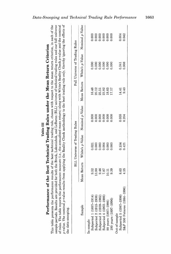
Table III presents the performance results of the best technical trading rule in each of the sample periods. The table reports the performance measure (i.e., mean return) along with White's Reality Checkp-value and the nominalp-value. The nominal p-value is that which results from applying the bootstrap methodology to the best trading rule only, thereby ignoring the effects of the data- snooping. Hence, the difference between the two p-values will represent the magnitude of the data-snooping bias on the performance measure.

Turning to the actual performance of the selected trading rules, first consider the results for the universe of 26 trading rules used by BLL. Both in the full sample and in the first four subperiods, we find that the apparent superior performance of the best trading rule stands up to a closer inspection for data-snooping effects. This finding is not surprising considering that every single one of BLL's trading rules outperforms the benchmark, and hence a consideration of dependencies between trading rules is unlikely to overturn their original finding.

Over the 100-year period from 1897 to 1996 the best technical trading rule from the BLL universe is a 50-day variable moving average rule with a 0.01 band, yielding an annualized return of 9.4 percent.14 For comparison, the

14 Annualized mean returns are calculated as the mean daily return over the duration of the sample, multiplied by 252. The mean daily return is simply the total return divided by the number of days in the sample.


PANEL A

0.01 1

0.008 | _ \ r-~~~~~~~BLL UniverseLX 0.008 -

- Full Universe

0.006-

0.004 -

0.002 -

1 2 3 4 5 6 7 8 9 10

Eigenvalue Number

PANEL B

0.0003 -

BLL Universe

0.00025 0.00025 0 0 -~~~~~~~~~~~~~Full Universe

0.0002 -

0.00015

0.0001- - X

0.00005

o Cr 00 - O in t e N O C cr 00 - o to v)t e c 0 Ci i I t in 00 Ol 0 o ci o -t tn v) t-o 00 cO 0

Eigenvalue Number

Figure 1. Span of the Brock, Lakonishok, and LeBaron (1992) universe of trading rules versus the full universe of trading rules: Eigenvalues 1 to 200 of the covariance matrix of returns. The eigenvalues of the covariance matrix of returns are sorted in descending order for the Brock, Lakonishok, and LeBaron (BLL) universe of trading rules (i.e., a 26 x 26 matrix), and for 500 randomly chosen rules from the full universe of trading rules (i.e., a 500 x 500 covariance matrix), including the 26 BLL rules. Panel A plots the 10 largest values in sorted descending order along the x-axis, where the y-axis measures the eigenvalue. Panel B plots eigenvalues 11 to 200, again sorted in descending order.

mean annualized return on the buy-and-hold strategy is 4.3 percent during this same period. In our full universe, the best trading rule chosen by the mean return criterion is a standard five-day moving average rule. The average annual return resulting from this rule is 17.2 percent. The Reality Check p-value is effectively zero (i.e., less than 1/B = 0.002), strongly indi-


Table I

Best

Technical

Trading

Rules

under

the

Mean

Return

Criterion

This

table

reports

the

historically

best-performing

trading

rule,

chosen

with

respect to

the

mean

return

criterion, in

each

sample

period

for

both of

the

trading

rule

universes:

the

Brock,

Lakonishok,

and

LeBaron

(1992)

(BLL)

universe

with

26

rules

and

our

full

universe

with

7,846

rules.

Sample

BLL

Universe of

Trading

Rules

Full

Universe of

Trading

Rules

In-sample Subperiod 1

(1897-1914)

50-day

variable

moving

average,

0.01

band

5-day

support &

resistance,

0.005

band,

5-day

holding

period

Subperiod 2

(1915-1938)

50-day

variable

moving

average,

0.01

band

5-day

moving

average

Subperiod 3

(1939-1962)

50-day

variable

moving

average,

0.01

band

2-day

on-balance

volume

Subperiod 4

(1962-1986)

150-day

variable

moving

average

2-day

on-balance

volume

90

years

(1897-1986)

50-day

variable

moving

average,

0.01

band

5-day

moving

average

100

years

(1897-1996)

50-day

variable

moving

average,

0.01

band

5-day

moving

average

Out-of-sample Subperiod 5

(1987-1996)

200-day

variable

moving

average,

0.01

band

Filter

rule,

0.12

position

initiation,

0.10

position

liquidation

S&P

500

Futures

(1984-1996)

200-day

variable

moving

average

30-

and

75-day

on-balance

volume


Table II

Best

Technical

Trading

Rules

under

the

Sharpe

Ratio

Criterion

This

table

reports

the

historically

best-performing

trading

rule,

chosen

with

respect to

the

Sharpe

ratio

criterion, in

each

sample

period

for

both

of

the

trading

rule

universes:

the

Brock,

Lakonishok,

and

LeBaron

(1992)

(BLL)

universe

with 26

rules

and

our

full

universe

with

7,846

rules.

Sample

BLL

Universe of

Trading

Rules

Full

Universe of

Trading

Rules


(1897-1914)

150-day

trading

range

break-out

20-day

channel

rule,

0.075

width,

5-day

holding

period

Subperiod 2

(1915-1938)

50-day

variable

moving

average,

0.01

band

5-day

moving

average,

0.001

band

Subperiod 3

(1939-1962)

50-day

variable

moving

average,

0.01

band

2-day

moving

average,

0.001

band

Subperiod 4

(1962-1986)

2

and

200-day

fixed

moving

average,

2-day

moving

average,

0.001

band

10-day

holding

period

90

years

(1897-1986)

50-day

variable

moving

average,

0.01

band

5-day

moving

average,

0.001

band

100

years

(1897-1996)

50-day

variable

moving

average,

0.01

band

5-day

moving

average,

0.001

band


(1987-1996)

150-day

fixed

moving

average,

10-day

holding

period

200-day

channel

rule,

0.150

width,

50-day

holding

period

S&P

500

Futures

(1984-1996)

200-day

fixed

moving

average,

0.01

band,

20-day

channel

rule,

0.01

width,

10-day

holding

period

10-day

holding

period


Table

III

Performance of

the

Best

Technical

Trading

Rules

under

the

Mean

Return

Criterion

This

table

presents

the

performance

results of

the

best

technical

trading

rule,

chosen

with

respect to

the

mean

return

criterion, in

each of

the

sample

periods.

Results

are

provided

for

both

the

Brock,

Lakonishok,

and

LeBaron

(BLL)

universe of

technical

trading

rules

and

our

full

universe

of

rules.

The

table

reports

the

performance

measure

(i.e.,

the

annualized

mean

return)

along

with

White's

Reality

Check

p-value

and

the

nominal

p-value.

The

nominal

p-value

results

from

applying

the

Reality

Check

methodology to

the

best

trading

rule

only,

thereby

ignoring

the

effects of

the

data-snooping.

BLL

Universe of

Trading

Rules

Full

Universe of

Trading

Rules

Sample

Mean

Return

White's

p-Value

Nominal

p-Value

Mean

Return

White's

p-Value

Nominal

p-Value


(1897-1914)

9.52

0.021

0.000

16.48

0.000

0.000

Subperiod 2

(1915-1938)

13.90

0.000

0.000

20.12

0.000

0.000

Subperiod 3

(1939-1962)

9.46

0.000

0.000

25.51

0.000

0.000

Subperiod 4

(1962-1986)

7.87

0.004

0.000

23.82

0.000

0.000

90

years

(1897-1986)

10.11

0.000

0.000

18.65

0.000

0.000

100

years

(1897-1996)

9.39

0.000

0.000

17.17

0.000

0.000


(1987-1996)

8.63

0.154

0.055

14.41

0.341

0.004

S&P

500

Futures

(1984-1996)

4.25

0.421

0.204

9.43

0.908

0.042


cating that trading with the five-day moving average is superior to being out of the market. In all four subperiods we find again that the best trading rule outperforms the benchmark strategy generating data-snooping adjusted p-values less than 0.002. Furthermore, the mean return of the best trading rule in the full universe tends to be much higher than the mean return of the best trading rule considered by BLL.

Considering next the full universe of trading rules from which, over time, the BLL rules are more likely to have originated, notice that two possible outcomes can occur when an additional trading rule is inspected. If the mar- ginal trading rule does not lead to an improvement over the previously best- performing trading rule, then the p-value for the null hypothesis that the best model does not outperform will increase, effectively accounting for the fact that the best trading rule has been selected from a larger set of rules. On the other hand, if the additional trading rule improves on the maximum performance statistic, then the p-value may decrease because better performance increases the probability that the optimal model genuinely contains valuable economic information.15

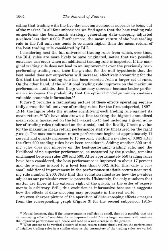
Figure 2 provides a fascinating picture of these effects operating sequen- tially across the full universe of trading rules. For the first subperiod, 1897- 1914, the figure plots the number identifying each trading rule against its mean return.16 We have also drawn a line tracking the highest annualized mean return (measured on the left y-axis) up to and including a given number of trading rules (indicated on the x-axis), and the Reality Check p-value for the maximum mean return performance statistic (measured on the right y-axis). The maximum mean return performance begins at approximately 11 percent and quickly increases to 15 percent, yielding a p-value of 0.002 after the first 200 trading rules have been considered. Adding another 300 trading rules does not improve on the best-performing trading rule, and the likelihood of no superior performance, as measured by the p-value, remains unchanged between rules 200 and 500. After approximately 550 trading rules have been considered, the best performance is improved to about 17 percent and the p-value is kept to a level less than 0.002. After this, only a very small additional improvement in the performance statistic occurs near trading rule number 2,700. Note that this evolution illustrates how the p-values adjust as our particular exercise proceeds. Ultimately, the only numbers that matter are those at the extreme right of the graph, as the order of experiments is arbitrary. Still, this evolution is informative because it suggests how the effects of data-snooping may propagate in the real world.

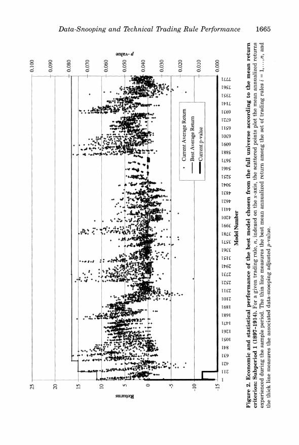
An even sharper picture of the operation of data-snooping effects emerges from the corresponding graph (Figure 3) for the second subperiod, 1915-

15 Notice, however, that if the improvement is sufficiently small, then it is possible that the data-snooping effect of searching for an improved model from a larger universe will dominate the improved performance and hence will lead to a net increase in the p-value.

16 What appear to be vertical clusters of mean return points simply reflect the performance of neighbor trading rules in a similar class as the parameters of the trading rules are varied.


25

0.100 0.090

20

0.080

15

++

++

10

+~~~~~~~

40

+4

++

4+

+ #1

+

*'**+ +

0.060

+

+

+1 +~~

004

+

+

~~~~~~~++

CretA

eaeRtr

.2

-10

-Bet

veageReur

+

+ ++

++

++*

+

~~~~~~~~~Crrntp-ale0.010

-15 ~

k

-

.

.0.000

!W

cic

ci

-:*

l-

r-+-

++

+

IA +

44~~~~~Mde

Number

#

Figure 2

Economi

an

ttsia

promneo

tebs

oe

chsnfo

h

uluies

acrigt

henrtr

crtron

upeid1

19-11)

oragve

rdigrle

,inee

n h

-ai,th

cttrdponspottemenanulzd

eun

exeincddrigte

apepeid

Tetinln

maue

tebstma

anaiedrtrnaog h

eto

rdigrle

1n

n

th tic

in

maurs h

asoite

dtasooin

djstdp-ale


25

0.100

20

~~~~~~~~~~~~~~~~~~~~~~~~~~~~~~~~0.090

20-

l

+F

F

;

0.080

15

l

F

$

$

+

+

+

* ;

* *

+~

+~~*:

~

++

++ +

+

0.030

It

**

.#4 ++

I

+

4

-10 -, *

$

.

Best

+Average

Return

l

l

|

*

~~~~~~~~~~~~~~

~~~Current

p-value

0.010ol

-15

_

0.000

(1

00

Cl

00

N4 O4

V4

N4 C4

Cl

00

Cl

00

_et

N

N t 4 oo O(1

N

(1(

?c

t

m

t-

?i

tl

m

i

>

N? N

N

N t<?

Model

Number

Figulre 3.

Economic

and

statistical

performance

of

the

best

model

chosen

from

the

full

universe

according to

the

mean

return

criterion:

Subperiod 2

(1915-1938).

For a

given

trading

rule, n,

indexed

on

the

x-axis,

the

scattered

points

plot

the

mean

annualized

returns

experienced

during

the

sample

period.

The

thin

line

measures

the

best

mean

annualized

return

among

the

set of

trading

rules i =

1,.n.,n

and

the

thick

line

measures

the

associated

data-snooping

adjusted

p-value.


1938. For this period, the best performing model is selected early on and remains in effect across the first 500 models. As a result, its p-value increases from 0.01 to 0.097 as more models are considered. After this, the addition of a model that improves the mean performance to 20 percent causes the p-value to drop to less than 0.002. Only at approximately rule 4,250 does the p-value increase marginally as no more improvements occur and the effective span of trading rules is increased.

A further issue at stake is how a trader could have possibly determined the best technical trading rule prior to committing money to a given rule. Although it may be the case that we are able to find the historically best- performing rule in our universe, there is no indication that it is possible to find ex ante the trading rule that will perform best in the future. To address this issue we consider a new trading strategy whereby on each day of the experiment we first determine the best-performing trading rule to date. That is, we find the rule with the greatest cumulative wealth for each day in the 100-year sample, and then follow the signal of that rule on the following day. At each point in time only historically available information is exploited so this trading rule could have been implemented by an investor.

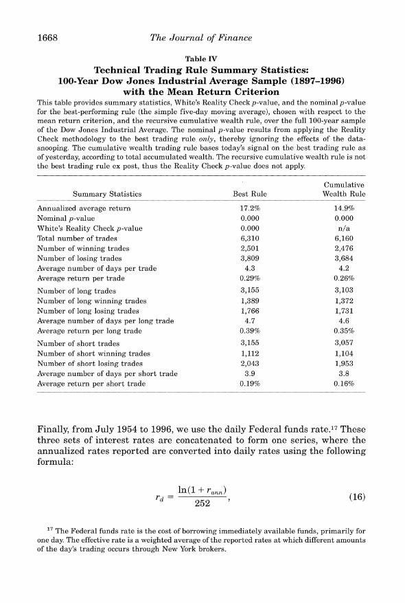
The results of this experiment are provided in Table IV, along with summary statistics for the best-performing technical trading rule chosen with respect to the mean return criterion, the five-day simple moving average. Table IV shows that the recursive cumulative wealth trading rule described above outperforms the benchmark with a 14.9 percent annualized average return, but lags behind the five-day moving average by more than two percentage points, reflecting the fact that investors could not have known ex ante the identity of the ex post best-performing trading rule. It is interesting to see that the number of short and long trades is roughly balanced out and that the winning percentage is much higher for the long than for the short trades. Long trades are also associated with average profits that are more than twice as large as those on the short trades.

B. Results for the Sharpe Ratio Criterion

Proper construction of the Sharpe ratio requires excess returns to be measured, where excess returns are the returns from the technical trading rule less the risk-free interest rate. The available data on daily risk-free interest rates is limited so we employ data from three separate sources for three overlapping periods. From 1897 to 1925, we use the interest rate for 90-day stock exchange time loans as reported in Banking and Monetary Statistics, 1914-1941 (1943). These rates are reported on a monthly basis and we convert them into a daily series by simply applying the interest rate reported for a given month to each day of that month. From 1926 to June 1954, we use the one-month T-bill rates reported by the Center for Research in Secu- rity Prices at the University of Chicago in their risk-free rates file. As these are also reported on a monthly basis, we convert them in the same way.


Table IV Technical Trading Rule Summary Statistics:

100-Year Dow Jones Industrial Average Sample (1897-1996) with the Mean Return Criterion

This table provides summary statistics, White's Reality Check p-value, and the nominal p-value for the best-performing rule (the simple five-day moving average), chosen with respect to the mean return criterion, and the recursive cumulative wealth rule, over the full 100-year sample of the Dow Jones Industrial Average. The nominal p-value results from applying the Reality Check methodology to the best trading rule only, thereby ignoring the effects of the data- snooping. The cumulative wealth trading rule bases today's signal on the best trading rule as of yesterday, according to total accumulated wealth. The recursive cumulative wealth rule is not the best trading rule ex post, thus the Reality Check p-value does not apply.

Cumulative Summary Statistics Best Rule Wealth Rule

Annualized average return 17.2% 14.9% Nominal p-value 0.000 0.000 White's Reality Check p-value 0.000 n/a Total number of trades 6,310 6,160 Number of winning trades 2,501 2,476 Number of losing trades 3,809 3,684 Average number of days per trade 4.3 4.2 Average return per trade 0.29% 0.26%

Number of long trades 3,155 3,103 Number of long winning trades 1,389 1,372 Number of long losing trades 1,766 1,731 Average number of days per long trade 4.7 4.6 Average return per long trade 0.39% 0.35%

Number of short trades 3,155 3,057 Number of short winning trades 1,112 1,104 Number of short losing trades 2,043 1,953 Average number of days per short trade 3.9 3.8 Average return per short trade 0.19% 0.16%

Finally, from July 1954 to 1996, we use the daily Federal funds rate.17 These three sets of interest rates are concatenated to form one series, where the annualized rates reported are converted into daily rates using the following formula:

In (1 + rann) rd

252 (16)

17 The Federal funds rate is the cost of borrowing immediately available funds, primarily for one day. The effective rate is a weighted average of the reported rates at which different amounts of the day's trading occurs through New York brokers.


where rd is the daily interest rate, rann is the reported annualized rate, and 252 represents the average number of trading days in a year.18

Since the volatility of daily interest rates is substantially smaller than that of daily stock returns, the main effect of including the risk-free rate in the Sharpe ratio is that of a (time-varying) drift-adjustment. For this reason, our use of monthly interest rates in the earlier samples is unlikely to affect the results in any important way.

Similar to Table III, Table V presents the performance results of the best technical trading rule in each of the sample periods. The table reports the performance measure (i.e., Sharpe ratio) along with White's Reality Check p-value and the nominal p-value.19

It is clear from Table II that the trading rules selected from the full universe by the Sharpe ratio criterion again tend to be based on a relatively short sample using two to 20 days of price information. Table V shows that the best model according to the Sharpe ratio criterion generates a p-value below 0.002 in all but one of the samples for the full universe of trading rules. Interestingly, the best model chosen from the BLL universe does not appear to be significant in several of the sample periods. Also, the performance of the best rule in the full universe increases substantially relative to the best rule considered by BLL. Over the full 100-year sample on the DJIA, the Sharpe ratio for the buy-and-hold strategy is a mere 0.034, but the best- performing trading rule in the BLL and full universe produces Sharpe ratios of 0.39 and 0.82, respectively.

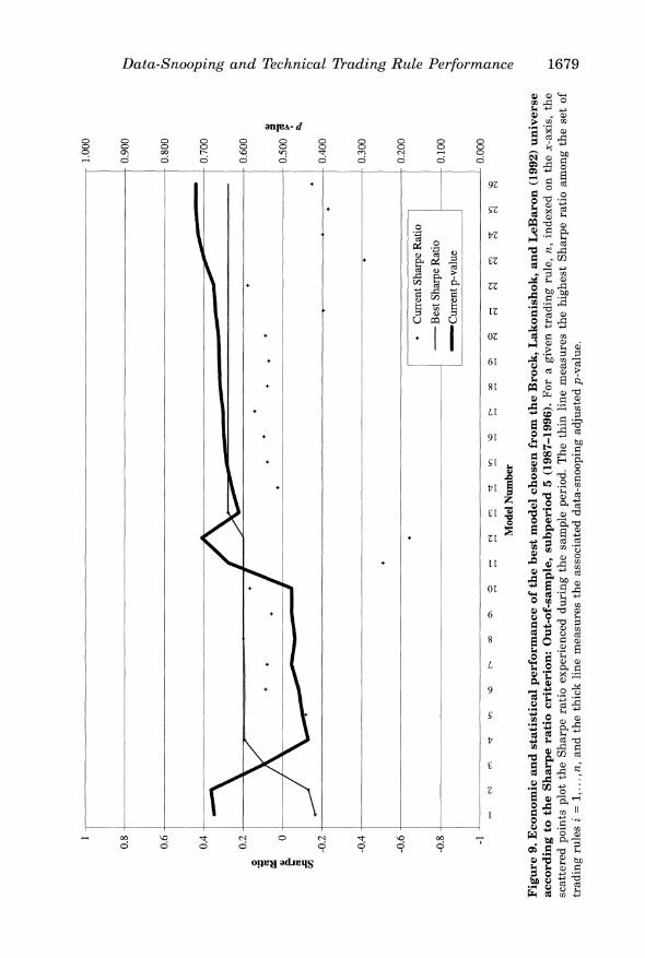
For the first two subperiods, Figure 4 and Figure 5 plot the sequence of Sharpe ratios based on the full set of models in contention alongside the p-value for the null that the highest Sharpe ratio equals zero. The most interesting graph appears for the second subperiod (Figure 5). The maximum Sharpe ratio is initially about 0.44. As the first 500 models get inspected, the p-value increases from 0.05 to above 0.60, only to fall well below 0.01 after a superior trading rule is introduced around model number 500. The p-value then increases from close to zero to a level around 0.056, thus displaying the effects of data-snooping as no improvements occur in the Sharpe ratio despite a widening of the span of trading rules.

These experiments also suggest why the alternative procedure of using a simple Bonferroni bound to assess the significance of the best-performing trading rule would give misleading results. Since the performance of the best trading rule drawn from the full universe is not known when considering only a subset of trading rules, the Bonferroni bound on the p-value

18 Examining the behavior of our interest rates in the first overlapping period (1925-1941, 193 observations), we find that monthly values for the stock exchange 90-day time loans and the Fama/Bliss risk-free rates have a correlation of 0.964. To compare the Fama/Bliss risk-free rates (monthly) to the Federal funds rates (daily), we convert the risk-free rates to daily rates by applying the Fama/Bliss rate for a given month to all days in that month. The overlap period of 1954-1996 (15,525 observations) produces a correlation of 0.963.

19 The Sharpe ratio values are based on annualized returns that are calculated as the continuously compounded daily return multiplied by 252.


Table V

Performance of

the

Best

Technical

Trading

Rules

under

the

Sharpe

Ratio

Criterion

This

table

presents

the

performance

results of

the

best

technical

trading

rule,

chosen

with

respect to

the

Sharpe

ratio

criterion, in

each of

the

sample

periods.

Results

are

provided

for

both

the

Brock,

Lakonishok,

and

LeBaron

(1992)

(BLL)

universe of

technical

trading

rules

and

our

full

universe of

rules.

The

table

reports

the

performance

measure

(i.e.,

the

Sharpe

ratio)

along

with

White's

Reality

Check

p-value

and

the

nominal

p-value.

The

nominal

p-value

results

from

applying

the

Reality

Check

methodology to

the

best

trading

rule

only,

thereby

ignoring

the

effects of

the

data-snooping.

BLL

Universe of

Trading

Rules

Full

Universe of

Trading

Rules

Sample

Sharpe

Ratio

White's

p-Value

Nominal

p-Value

Sharpe

Ratio

White's

p-Value

Nominal

p-Value


(1897-1914)

0.51

0.147

0.016

1.15

0.000

0.000

Subperiod 2

(1915-1938)

0.51

0.037

0.000

0.76

0.056

0.000

Subperiod 3

(1939-1962)

0.79

0.000

0.000

2.18

0.000

0.000

Subperiod 4

(1962-1986)

0.53

0.051

0.003

1.41

0.000

0.000

90

years

(1897-1986)

0.45

0.000

0.000

0.91

0.000

0.000

100

years

(1897-1996)

0.39

0.000

0.000

0.82

0.000

0.000


(1987-1996)

0.28

0.721

0.127

0.87

0.903

0.000

S&P

500

Futures

(1984-1996)

0.23

0.702

0.165

0.66

0.987

0.000


1.5

0.100 0.090

1

~~~~~~~~~~~~~~~~~~~~~~~~~~~~~~~~0.080

1*4.

Z+

~ +;

4

4.

00.5

~+

+

.4

+

* +

+

+~4*

$

+4

*4.

+

+~~*v~

+

..4

+4.4

+

+

4

'I

..

4;.4

+

'

+

4.

4.

4.-0'O.

+

*,+

++ +

~

+ +

+

?j4

+

~~~~~ .44t

*+

:s~~~~~~~~~~~~~~~~~#~+

++

+

44.4*+

0.5+

0.040

+*+4

f~

++

+

1

+.+4

+

0.3

+

.~~~~~4*+~.4.+4$

.2

+4

+~~~4.t~ 444 *+

4.

4.

4.

4.4.

*+

+.

V +

~~~~~~~~~~~~~~~~0.000

Ci0

I0 N

i~

0

)

C)

o

C

)

~

~

C

~ 0

0

i~

0

0)

C)~

-

)

1)~

0

.0

4

Ci+

+i

C

i

C

'

'

'

'

t~

t~

t

L)~

)~

)

~

~

C~C

-

-

4

I~~~~~~oelNme

Fiur .

cooican

taisialprfrmne

f h

bstmde

hoenfomth

ul

uiereacorig

o

h

Sarerai

crteio:

upeio

1(89-114.Fo

agientadngrue n

idee

ontexai,tesatrdpit

ltteSap

ai

xeine

durig th

samle

priod

The1

thnln

esrste

ihs

hrerto

mn

h

e

ftain

ue

.,adth

hc

iemaue

th

sscaeddt-sopngajstdpvau.Noetatpvlusgrae

ta

.1

ae

entrnaeda

hetpoftefiue


1.5

1

0.100 0.090

1

0.080 0.070

0.5

+

.+

o,o

+ +

~

4+

1

+

+ +

++

~~~~~~~~~~++

+

~

+~

.5

5

t

S00

.

0503~~~~~~~~~~~~~~~~~~~~~~~~~~~~~.4

*

4+

+:+

+

*+4*

~

+

?

ie

+

++*

~ 4

.3

-0

5

r--

-->

r

*X

---

1

.~~~~~~~~~~~~

Current

Sharpe

Ratio

-0.020

+

$

*

- -

+Currentp-value

0.010

- 1

- .

...

_

.

.,_I'

0.000

(N

m

t

00

xo

>

o

oc t m-

00

C\

o

N

m

00

C\

o

tO

mO

?

00

oi

tO

?

00

0

C tO

?

Ch

00

C

Ct

v

? t O

N

t-

00m

C\

oS

tO

C>N t~

00

O~ F e

C

~t t1

00

t3

to

n

o

m

en

C

00

t

tO

t

C\

)

tO

00

???

Model

Number

Figure 5.

Economic

and

statistical

performance

of

the

best

model

chosen

from

the

full

universe

according

to

the

Sharpe

ratio

criterion:

Subperiod 2

(1915-1938).

For a

given

trading

rule, n,

indexed

on

the

x-axis,

the

scattered

points

plot

the

Sharpe

ratio

experienced

during

the

sample

period.

The

thin

line

measures

the

highest

Sharpe

ratio

among

the

set of

trading

rules i

=1,...,n,

and

the

thick

line

measures

the

associated

data-snooping

adjusted

p-value.

Note

that

p-values

greater

than

0.10

have

been

truncated at

the

top of

the

figure.


cannot possibly be used to account for data-snooping. A researcher might believe that, say, the BLL trading rules are the result of traders considering an original set of 8,000 rules, in which case the Bonferroni bound on the p-value would be obtained as 8,000 times the smallest nominal p-value. But this leads to meaningless results: In subperiod 4, the Bonferroni bound simply states that the p-value is less than 1, but in fact the bootstrap p-value for the best trading rule selected from the full universe is approximately 0.05.

C. Performance of the Bootstrap Snooper

In this subsection we carry out a simple check on the performance of White's Reality Check methodology by comparing the actual performance measure fk

to the bootstrapped values of the performance measure ft,i, for k = 1,...,1

trading rules and i = 1,...,B bootstrap samples (1 = 7,846 and B = 500).20

The results are displayed in Figures 6 and 7. For each of the k models and for both the mean return and Sharpe ratio criteria applied to the 100-year DJIA sample, these figures provide a histogram of the realized probability that j,7i is greater than fk across the full universe of trading rules. Note that the distribution is closely centered around one-half, suggesting that White's Reality Check methodology is performing as it should. Also, the results are very similar for both performance measures.21

Calculation of the overall probability, across all trading rules and bootstrap samples, that f&,i exceeds fk yields a value of 0.489 for both the mean return and Sharpe ratio criteria. Omitting outliers caused by infrequent trading yields a probability of 0.508 for both performance measures.

D. The Effects of Nonsynchronous Thading

Another issue to consider is nonsynchronous trading. If some of the closing prices on the DJIA are stale, they may not reflect the latest information. In such a case, the technical trading rules and the cumulative wealth rule would not be able to obtain the closing price when the markets open the following day. Although nonsynchronous trading effects are likely to be relatively small for the stocks included in the DJIA, it is possible that some do exist, especially on low volume days.22 To address this issue, we follow Ready (1997)

20 We thank an anonymous referee for suggesting this analysis. 21 There is a set of outlier models, about 300 trading rules, that have a probability at, or

near, zero that f1*lj will exceed fk. This is a result of a trading rule having very few nonzero trading signals. In such a case, it is entirely possible that none of the 500 bootstrap samples will include any nonzero signals, thereby leading to a bootstrapped performance measure that is always less than the actual performance measure that does contain some nonzero trading signals. This is clearly not a problem for the results reported in Tables I-VI because the selected trading rules generate multiple signals.

22 For example, Campbell, Grossman, and Wang (1993) find that the first-order autocorre- lation in daily stock returns is higher when volume is low.


1,600 . ..... 8 w ........ .8 8... .8 8.8 .v z.v....... .8...... ............ ..8 8. .8...

1,400. * . *- .

1,200

e 1,000 - _ ______- _

48 800 - - - - ---- - _ _

400 -- _ _ _ _ _

200

0.00 0.42 0.43 0.44 0.45 0.46 0.47 0.48 0.49 0.50 0.51 0.52 0.53 0.54 0.55 0.56 0.57 0.58 1.00

Probability Range

Figure 6. Histogram of the observed probability that the bootstrapped performance measure is greater than the actual performance measure, according to the mean return criterion: 100-year sample (1897-1996). The observed probability is the number of bootstrap samples yielding a performance measure greater than the actual performance measure, divided by the number of bootstrap samples (500). For a given probability range, the y-axis measures the number of models (trading rules) from the full universe of 7,846 rules that have a calculated probability within that range. The x-axis value, the probability range, indicates the upper bound on the range of probability values, where the lower bound is provided by the next smaller upper bound.

and let a trading signal observed on day t be implemented on the following day, t + 1. We then perform the bootstrap experiment on the full universe of trading rules and the 100-year DJIA sample using the delayed signals.

The results are quite interesting. The best rule according to the mean return criterion is a variable moving average with a band filter where the fast moving average is calculated over two days, the slow moving average is calculated over 75 days, and a 0.001 band is applied. For the Sharpe ratio criterion, the best rule is a fixed moving average with a fast MA of 20 days, a slow MA of 75 days, and a fixed holding period of five days. Not surpris- ingly, the best rules in this experiment are of a longer duration than those where the trading signals are implemented immediately.

The mean return of the best rule is 7.8 percent with a Reality Check p-value of nearly zero (i.e., less than 0.002), indicating that the best rule is still highly significant. Note that this is true even though the performance is far less than the best from the standard experiment of 17.2 percent. The Sharpe ratio of the best rule is 0.34 with a Reality Checkp-value of 0.26, suggesting that the best rule, according to the Sharpe ratio criterion, is no longer significant.23

23 Ready (1997) also finds that what he refers to as "price slippage" effects can account for a substantial part of the profits generated by technical trading rules.


1,600 -

1,400 -

1,200 -__

1 800 |

Z600-

400-

200 -

0.00 0.42 0.43 0.44 0.45 0.46 0.47 0.48 0.49 0.50 0.51 0.52 0.53 0.54 0.55 0.56 0.57 0.58 1.00

Probability Range

Figure 7. Histogram of the observed probability that the bootstrapped performance measure is greater than the actual performance measure, according to the Sharpe ratio criterion: 100-year sample (1897-1996). The observed probability is the number of bootstrap samples yielding a performance measure greater than the actual performance measure, divided by the number of bootstrap samples (500). For a given probability range, the y-axis measures the number of models (trading rules) from the full universe of 7,846 rules that have a calculated probability within that range. The x-axis value, the probability range, indicates the upper bound on the range of probability values, where the lower bound is provided by the next smaller upper bound.

One further item of interest is the performance of the cumulative wealth rule under this regime. The cumulative wealth rule manages to outperform the benchmark with a mean return of 4.6 percent. The nominal p-value is nearly zero (i.e., less than 0.002).

V. Out-of-Sample Results

The data used in the study by BLL finish in 1986. This leaves us with a 10-year postsample period in which a genuine out-of-sample performance experiment can be conducted. We do so using the Dow Jones portfolio originally studied by BLL, and we also use prices on the S&P 500 Futures contract that has traded since 1984 and hence covers a commensurate period. Lo and MacKinlay (1990) recommend just such a 10-year out-of-sample experiment as a way of purging the effects of data-snooping biases from the analysis.

There is a distinct advantage associated with using the futures data set: The experiment on the DJIA data ignores dividends (which are not available on a daily basis for the full 100-year period), but these are not a concern for the futures contract. Furthermore, although the assumption that investors


could have taken short positions in the DJIA contract throughout the entire period 1897-1996 may not be realistic, it would have been very easy for an investor to have gone short in the S&P 500 Futures contract. Finally, it is possible that the technical trading rules considered by BLL generated profits before transaction costs, but accounting for such costs and data-snooping effects could change their findings.24 In the full universe and over the 100- year period 1897-1996, the best-performing trading rule for the DJIA earned a mean annualized return of 17.17 percent resulting from 6,310 trades (63.1 per year), giving a break-even transaction cost level of 0.27 percent per trade. We do not have historical series on transaction costs, and these would also seem to depend on the size of the trade, so it seems difficult to assess this number. Transaction costs are likely to have been higher than 0.27 percent at the beginning of the sample, but lower by the end of the sample. Ulti- mately, the transaction cost argument is best evaluated using a trading strategy in a futures contract, such as the S&P 500, where transactions costs are quite modest.

The S&P 500 Futures data are provided by Pinnacle Data Corporation. The prices from the nearest futures contract are employed with a rollover date of the 9th of the delivery month for the contract. That is, any position maintained in the current contract is closed out, and a new position is opened, according to the trading rule, on the 9th of March, June, September, and December. A series of returns is created from each of the contracts and is linked together at the rollover dates. Starting with the price of the S&P 500 Futures contract at the beginning of the series, a new price series is generated from the returns.

A quick first way of testing the merits of technical trading rules is by considering the performance of the best trading rule, selected by the end of 1986, in the subsequent 10-year trading period. The five-day moving average rule selected from the full universe produces a mean return of 2.8 percent with a nominal p-value of 0.322 for the period 1987 to 1996, indicating that the best trading rule, as of the end of 1986, did not continue to generate valuable economic signals in the subsequent 10-year period.

Figure 8 presents graphs for the evolution in the maximum performance statistic and the Reality Check p-value across the 26 trading rules considered by BLL applied to the out-of-sample period. The third and fourth trading rules improve substantially on the maximum mean return statistic and the addition of these rules leads to decreases in the p-value. By the end of the sample, the maximum mean return statistic is approximately 8.5 percent per year. The p-value starts out near 0.3, decreases to about 0.13, but then slowly increases to 0.15. Such increases in the p-value, in the absence of improvements over the best performing trading rule, vividly illustrate the

24 In the conclusion to their paper, BLL call for careful consideration of transaction costs and explicitly recommend using futures data as a way of dealing with this issue. This is particularly important for some of the rules selected from the full universe which use very short windows of the data, generate very frequent trading signals, and hence are likely to generate substantial transaction costs.


15-

1.000

+

Current

Average

Return

-Best

Average

Retumr

0.900

Current

p-value

10 -

0.800 0.700

5-

0.600

0 -

+

0.500 D

0.400

-5-

0.300 0.200

-10 -

0.100

-15 -

0.000

C"O

m

00

C

0

N

00

C9

0

Model

Number

Figure 8.

Economic

and

statistical

performance

of

the

best

model

chosen

from

the

Brock,

Lakonishok,

and

LeBaron

(1992)

universe

according to

the

mean

return

criterion:

Out-of-sample,

subperiod 5

(1987-1996).

For a

given

trading

rule, n,

indexed

on

the

x-axis,

the

scattered

points

plot

the

mean

annualized

returns

experienced

during

the

sample

period.

The

thin

line

measures

the

best

mean

annualized

return

among

the

set of

trading

rules i =

1,...,n,

and

the

thick

line

measures

the

associated

data-snooping

adjusted

p-value.


importance of jointly considering all the trading rules when drawing conclusions about the performance of the best-performing trading rule. The p-value for the best-performing trading rule, considered in isolation, is 0.05. The evidence that the best trading rule can produce superior performance is even weaker when the Sharpe ratio criterion is used to measure performance. For this criterion, the p-value of the best model chosen from the BLL universe terminates at 0.72 when data-snooping is accounted for (see Figure 9) and is 0.12 when the trading rule is naively considered in isolation.

Consider next the full universe of 7,846 trading rules for the S&P 500 Futures data over the period 1984-1996. For models selected by the mean return criterion, Figure 10 demonstrates perhaps more clearly than any other graph the importance of controlling for data-snooping. After the first few trading rules are considered, the p-value falls to around 0.3, but it quickly increases to around 0.6 as no improvement over the best-performing trading rule occurs until after approximately 400 trading rules. Then the p-value drops back below 0.4 only to increase to a level around 0.9 by the point the final trading rule has been evaluated. As is clear from Figure 11, a very similar picture emerges for the Sharpe ratio criterion, where the terminal data-snooping-adjusted p-value is 0.99.

Notice the very strong conclusion we can draw from this finding. Even though a particular trading rule is capable of producing superior performance of almost 10 percent per year during this sample period and has a p-value of 0.04 when considered in isolation, the fact that this trading rule is drawn from a wide universe of rules means that its effective data-snooping- adjusted p-value is actually 0.90. An even bigger contrast occurs from using the Sharpe ratio criterion: here the snooping-adjusted and unadjusted p-values are 0.99 and 0.000 (below 0.002), respectively. Indeed, data-snooping effects are very important in assessing economic performance.

As a final exercise, we compute the out-of-sample performance of the recursive decision rule described in Section IV. This rule follows the trading signal generated by the rule that has produced the highest cumulative wealth as of the previous trading day. Table VI provides summary statistics for the best-performing rule and the cumulative wealth rule, for both the out-of- sample DJIA (1987-1996) and the Standard and Poor's 500 Futures (1984- 1996). These rules are chosen with respect to the mean return criterion. It is interesting to note that in both of these out-of-sample periods the cumulative wealth rule does not perform well. In fact, the cumulative wealth rule applied to the S&P 500 Futures generates negative returns. Also, note that the best rule for the DJIA results in only six trades, where each trade averages over 400 days. This is considerably greater than the average of 4.3 days per trade resulting from the best rule over the full 100-year sample.

VI. Conclusion

This paper applies a new methodology that allows researchers to control for data-snooping biases to compute the statistical significance of investment performance while accounting for the dependencies resulting from in-


1 -

1.000

0.8 -

-

0.900

0.6 -

-

0.800

0.4 -

0.700

0.2

+

+

0.600

o

~~~~~~~~~~~~~~~~~~~~~~~~~~~~~~~~~+

0 -

0.500

cI~~~~~~~~~~~~~~~~~~~~~~~~~~~~~~~~~~~~~~~

~~~~~~~~~~~~+

-0.2 -

0.400

-0.4

-+

-0.300

-0.6 -

-

0.200

t

Current

Sharpe

Ratio

-0.8 -

Best

Sharpe

Ratio

-

0.100

inCurrent

p-value

-1 -

-

0.000

-

c's

es

t

r-?

00

O~

cs

-

c'

v:

?

t

00

O\

o

c's

es

t :

Model

Number

Figure 9.

Economic

and

statistical

performance

of

the

best

model

chosen

from

the

Brock,

Lakonishok,

and

LeBaron

(1992)

universe

according

to

the

Sharpe

ratio

criterion:

Out-of-sample,

subperiod 5

(1987-1996).

For a

given

trading

rule, n,

indexed

on

the

x-axis,

the

scattered

points

plot

the

Sharpe

ratio

experienced

during

the

sample

period.

The

thin

line

measures

the

highest

Sharpe

ratio

among

the

set of

trading

rules i =

1.

n,

and

the

thick

line

measures

the

associated

data-snooping

adjusted

p-value.


15

.0 0.900

10

+

~

:

0.700

V

+

~ :

#::

.0

+

+

4

EI

.0

+

~ ~

~

*

~

~

? ~~

~+*s+#

+

+*

+

+

+

+

+

+~

~~~~~~~~~~~~~~~~

0.300

+

;+

+*~~~~~

*

*

5

+

+

~~~~~~~~~~~~~~+

+

+

urn

veaeRtr

+

+

~~~~~~~~~~~~~~~+

++

+

Bs

Aeae

eun

.0

++

+

in

uretp-au

-15

+

0.000~~~~~+

+4.+

+

ul + +40

++

Moel

Nmbe

Fiur

0.Eonmc

n

saisialprfrmne

fth

es

odlchsn

rm

h

flluivre

corig

oth

ea

etr

critrio:

SP 50

Fuure

(18-96.Fragvntain

ue

,idxdo

h

-ai,tesatrdpit

lo

h

enanaieeun

exerene

drig

h

smpe

eio.

hetinlie

esuesth

es

mananuliedrtun

mogth

st

ftrdig

uesi

!1n

ad h

thick

ine

mesuresthe asociatd datasnoopig

adjsted

pvalue


1

1|ESt

_

_

_

-

1

.

0

0

1.000

0.8

0.900

0.6

0.800

0.4

0.700

.

+

.

.

.~~~~~~~~~~+

+

+

+

0.2

-

+

+

+

0.600

+.

.+

++

+

+

+

0.

s._+

4

-

0.600

+,*

**$+

+

-0.2

+ +

'

*Ir

0.400

-1, -

+

. +

,,,

+

I+

+4.

+++

.

_ _ _ _

__$

+_ _ _ _

_. 0

-s

ce

t-

00

?

>

00

zON

Cl

eN

mt

-

00

ON

oc

cl

o~

Nt

m

-

00

oc

oN m

?>o

Cl~

~~~~~ o

00

Cl

>

O

ON

et

l

m-

o

00

du

C

t

?

ON

t~

m-

ON

t>

WO

0

ci

ci

ci

c

ci

e~

m

m

t

t

Wm

fm

fm

fm m

?>r

Model

Number

Figure

11.

Economic

and

statistical

performance

of

the

best

model

chosen

from

the

full

universe

according

to

the

Sharpe

ratio

criterion:

S&P

500

Futures

(1984-1996).

For a

given

trading

rule, n,

indexed on

the

x-axis,

the

scattered

points

plot

the

Sharpe

ratio

experienced

during

the

sample

period.

The

thin

line

measures

the

highest

Sharpe

ratio

among

the

set of

trading

rules i =

1,...,n,

and

the

thick

line

measures

the

associated

data-snooping

adjusted

p-value.


Table VI

Technical

Trading

Rule

Summary

Statistics:

Out-of-Sample

Dow

Jones

Industrial

Average

(1987-1996)

and

the

Standard

and

Poor's

500

Futures

(1984-1996)

with

the

Mean

Return

Criterion

This

table

provides

summary

statistics,

White's

Reality

Check

p-value,

and

the

nominal

p-value

for

the

best-performing

rule,

chosen

with

respect

to

the

mean

return

criterion,

and

the

recursive

cumulative

wealth

rule,

for

both

the

out-of-sample

Dow

Jones

Industrial

Average

(1987-1996)

and

the

Standard

and

Poor's

500

Futures

(1984-1996).

The

nominal

p-value is

that

which

results

from

applying

the

Reality

Check

methodology to

the

best

trading

rule

only,

thereby

ignoring

the

effects of

the

data-snooping.

The

cumulative

wealth

trading

rule

bases

today's

signal on

the

best

trading

rule as of

yesterday,

according to

total

accumulated

wealth.

The

recursive

cumulative

wealth

rule is

not

the

best

trading

rule ex

post,

thus

the

Reality

Check

p-value

does

not

apply.

Dow

Jones

Industrial

Average

S&P

500

Futures

Cumulative

Cumulative

Summary

Statistics

Best

Rule

Wealth

Rule

Best

Rule

Wealth

Rule

Annualized

average

return

14.4%

2.8%

9.4%

-5.5%

Nominal

p-value

0.000

0.322

0.042

0.895

White's

Reality

Check

p-value

0.341

n/a

0.908

n/a

Total

number of

trades

6

676

43

210

Number of

winning

trades

4

234

22

56

Number of

losing

trades

2

442

21

154

Average

number of

days

per

trade

411.7

3.7

76.5

14.3

Average

return

per

trade

34.38%

0.04%

3.00%

-0.33%

Number of

long

trades

4

338

22

104

Number of

long

winning

trades

3

140

12

31

Number of

long

losing

trades

1

198

10

73

Average

number of

days

per

long

trade

598.0

4.3

98.6

17.1

Average

return

per

long

trade

48.16%

0.24%

5.76%

0.16%

Number of

short

trades

2

338

21

106

Number of

short

winning

trades

1

94

10

25

Number of

short

losing

trades

1

244

11

81

Average

number of

days

per

short

trade

39.0

3.2

53.4

11.6

Average

return

per

short

trade

6.82%

-0.16%

0.12%

-0.82%


vestigating several investment rules. We believe that this methodology deserves to be widely used in finance: There is an obvious focus in finance on information and decision rules that can be used to predict financial returns, but it is often forgotten that this predictability may be the result of a large number of researchers' joint search for a successful model specification with predictive power. Many researchers, such as Merton (1987), have called for a remedy to control for data-snooping biases, and the methodology in this paper provides just such a tool. It summarizes in a single statistic the significance of the best-performing model after accounting for data-snooping.

Aside from being important in assessing the influence of data-snooping bias in performance measurement studies, the approach of this paper also has substantial value to investors who are searching for successful investment strategies. Suppose that, after experimenting with a large number of decision rules, an investor comes up with what appears to be a highly successful rule that outperforms the benchmark strategy. The investor is then left with the task of assessing just how much of the performance is a result of data-snooping, and how much is due to genuine superior performance. In the presence of complicated dependencies across the rules being evaluated, this is a very difficult question to answer, and only a bootstrap methodology such as the one offered in this paper appears to be feasible. Furthermore, since the investor would know the exact identity of the universe of investment rules from which the optimal rule is drawn, the approach of this paper is eminently suited for such an assessment.

Our analysis allows us to reassess previous results on the performance of technical trading rules. We find that the results of BLL appear to be robust to data-snooping, and indeed there are trading rules that perform even better than the ones considered by BLL. Hence their result that the best performing technical trading rule is capable of generating profits when applied to the DJIA stands up to inspection for data-snooping effects. This finding is valid in all four subperiods considered by BLL. However, we also find that the superior performance of the best technical trading rule is not repeated in the out-of-sample experiment covering the 10-year period 1987-1996. In this sample the results are completely reversed and the best-performing trading rule is not even statistically significant at standard critical levels. This result is also borne out when data on a more readily tradable futures contract on the S&P 500 index are considered: Again there is no evidence that any trading rule outperforms over the sample period.

Three conclusions appear to be possible from these findings. First, the out-of-sample results may simply not be representative, possibly because of the unusually large one-day movement occurring on October 19, 1987. Al- though this argument can never be rejected outright, we want to emphasize that the out-of-sample trading period is rather long (3,291 days), which would seem to lend support to the claim that we can evaluate the trading rules' performance reasonably precisely in the postsample period. Also, the out-of- sample results are robust to whether or not data on 1987 are included in the sample. In a finite sample, very large movements in stock prices such as


those occurring on October 19, 1987 would, if anything, actually tend to improve the performance of the best trading rule because some of the rules inevitably would have been short in the index on that date and hence would have earned returns of 22 percent in a single day.25

Second, the 7,846 trading rules that we consider may of course have been selected from an even larger universe of rules. If this is the case, then the p-value adjusted for data-snooping is biased toward zero under the assumption that the included rules are also the ones that performed quite well during the historical sample period. This explanation is a logical possibility, but the experiments reported in this paper also show that it can have merit only as long as two conditions are both satisfied: The omitted trading rules cannot improve substantially on the best-performing trading rule drawn from the current universe, and the omitted trading rules should generate payoffs that are largely orthogonal to the payoffs of the included trading rules so that they will increase the effective span. We think that we have been sufficiently careful in choosing the number and types of trading rules included in the adopted universe so that it is unlikely that these conditions are simultaneously satisfied.

Third, it is possible that, historically, the best technical trading rule did indeed produce superior performance, but that, more recently, the markets have become more efficient and hence such opportunities have disap- peared.26 This conclusion certainly seems to match up well with the cheaper computing power, the lower transaction costs and increased liquidity in the stock market that may have helped to remove possible short-term patterns in stock returns.

Appendix A. Trading Rule Parameters

This appendix describes the parameterizations of the 7,846 trading rules used to generate the full universe of rules under consideration.

A. 1. Filter Rules

x - change in security price (x x price) required to initiate a position; y = change in security price (y x price) required to liquidate a position; e = used for an alternative definition of extrema where a low (high) can be

defined as the most recent closing price that is less (greater) than the n previous closing prices;

25 Indeed, as shown in Table III, the best trading rule from the BLL universe under the mean return criterion generates a mean return of 8.6 percent in the period from January 1987 through December 1996. However, the best rule (200-day variable moving average with a 1 percent band) from the BLL universe in the period January 1988 through December 1996 generates a mean return of only 5.6 percent. Furthermore, the large universe provides a best rule during subperiod 5 that generates a mean return of 14.4 percent, whereas the best rule (20-day filter rule of 0.10) during the period beginning in 1988 provides a mean return of only 13.9 percent.

26 Ready (1997) also reports a decline in the ability of technical trading rules to predict daily returns over the period 1990-1995.


c = number of days a position is held, ignoring all other signals during that time;

x = 0.005, 0.01, 0.015, 0.02, 0.025, 0.03, 0.035, 0.04, 0.045, 0.05, 0.06, 0.07, 0.08, 0.09, 0.1, 0.12, 0.14, 0.16, 0.18, 0.2, 0.25, 0.3, 0.4, 0.5 [24 values];

y = 0.005, 0.01, 0.015, 0.02, 0.025, 0.03, 0.04, 0.05, 0.075, 0.1, 0.15, 0.2 [12 values];

e = 1, 2, 3, 4, 5, 10, 15, 20 [8 values]; c = 5, 10, 25, 50 [4 values].

Noting that y must be less than x, there are 185 x-y combinations.

Number of filter rules = x + (x * e) + (x * c) + (x-y combinations) = 24 + 192 + 96 + 185 = 497.

A.2. Moving Averages

n = number of days in a moving average; m = number of fast-slow combinations of n; b = fixed band multiplicative value; d = number of days for the time delay filter; c = number of days a position is held, ignoring all other signals during

that time; n = 2, 5, 10, 15, 20, 25, 30, 40, 50, 75, 100, 125, 150, 200, 250 [15 values];

n-1

m = i = 105; i~=1

b = 0.001, 0.005, 0.01, 0.015, 0.02, 0.03, 0.04, 0.05 [8 values]; d = 2, 3, 4, 5 [4 values]; c = 5, 10, 25, 50 [4 values].

Note that a 1 percent band filter and a 10-day holding period are applied to all combinations of moving averages with a fast MA of one, two, and five days and a slow MA of 50, 150, and 200 days. This addition of nine rules allows our universe of trading rules to encompass all of BLL's trading rules.

Number of rules = n + m + (b * (n + m)) + (d * (n + m)) + (c * (n + m)) + 9 = 15 + 105 + 960 + 480 + 480 + 9 = 2,049.

A.3. Support and Resistance

n = number of days in the support and resistance range; e = used for an alternative definition of extrema where a low (high) can

be defined as the most recent closing price that is less (greater) than the n previous closing prices;

b = fixed band multiplicative value; d = number of days for the time delay filter; c = number of days a position is held, ignoring all other signals during

that time; n = 5, 10, 15, 20, 25, 50, 100, 150, 200, 250 [10 values];


e = 2, 3, 4, 5, 10, 20, 25, 50, 100, 200 [10 values]; b = 0.001, 0.005, 0.01, 0.015, 0.02, 0.03, 0.04, 0.05 [8 values]; d = 2, 3, 4, 5 [4 values]; c = 5, 10, 25, 50 [4 values].

Number of rules [(1 + c) * (n + e)] + [(b * (n + e)) * (1 + c)] + [d * c * (n + e)] 100 + 800 + 320 = 1,220.

A.4. Channel Breakouts

n = number of days for the channel; x = difference between the high price and the low price (x x high price)

required to form a channel; b = fixed band multiplicative value; c = number of days a position is held, ignoring all other signals during

that time; n = 5, 10, 15, 20, 25, 50, 100, 150, 200, 250 [10 values]; x = 0.005, 0.01, 0.02, 0.03, 0.05, 0.075, 0.10, 0.15 [8 values]; b = 0.001, 0.005, 0.01, 0.015, 0.02, 0.03, 0.04, 0.05 [8 values]; c 5, 10, 25, 50 [4 values].

Noting that b must be less than x, there are 43 x-b combinations.

Number of rules - (n * x * c) + [n * b * (x-b combinations)] = 320 + 1,720 = 2,040.

A.5. On-Balance Volume Averages

n = number of days in a moving average; m = number of fast-slow combinations of n; b = fixed band multiplicative value; d = number of days for the time delay filter; c = number of days a position is held, ignoring all other signals during

that time; n = 2, 5, 10, 15, 20, 25, 30, 40, 50, 75, 100, 125, 150, 200, 250 [15 values];

n-1

m > i = 105; i=l1

b = 0.001, 0.005, 0.01, 0.015, 0.02, 0.03, 0.04, 0.05 [8 values]; d - 2, 3, 4, 5 [4 values]; c = 5, 10, 25, 50 [4 values].

Number of rules = n + m + (b * (n + m)) + (d * (n + m)) + (c * (n + m)) 15 + 105 + 960 + 480 + 480 = 2,040.

Appendix B. Reality Check Technical Results

For the convenience of the reader, we replicate the main results of White (1999) and briefly interpret these. In what follows, the notation corresponds to that of the text unless otherwise noted.


Let P denote the probability measure governing the behavior of the time series {Zt}. Also, =* denotes convergence in distribution, and 24 denotes convergence in probability. In White's (1999) notation, used here, f* f (Z, *) where j3 * plimn,8T. As no parameters are estimated in our application, we have written E ( f) in the text.

PROPOSITION 2.1: Suppose that n1/2( f-Ef*)) (f N(O,fl) for Q positive semi- definite. (a) If E(fk*), > 0 for some 1 c k ' 1, then for any 0 ? c < E(fk*), P[ fk > c] -- 1 as T -- oo. (b) IflI > l and E(ff*) > E(fk*), for all k = 2,..., 1, then P[f1 > fk for all k I2,...,] - 1 as T -o oo.

Part (a) says that if some model (e.g., the best model) beats the benchmark, then this is eventually revealed by a positive estimated relative performance. Part (b) says that the best model eventually has the best estimated performance relative to the benchmark, with probability approaching one. The next result provides the basis for hypothesis tests of the null of no predictive superiority over the benchmark, based on the predictive model selection criterion.

PROPOSITION 2.2: Suppose that n 1/2 ( E(f*)) =f N(O, f) for Ql positive semi- definite. Then as T -- oo

max n / {fk-E(fk,)} => Vi- max {Zk} (Bi)

and

min n {k- E(fk))}= WIk min {Zk}, (B2)

where Z is an I x 1 vector with components Zk, k 1,...,1, distributed as N(0, Ql).

COROLLARY 2.4: Under the conditions of Theorem 2.3 of White (1999), we have that as T -- oc

p(L[V,*|Z1, . .. ,ZT+J , LI max n /( fk -E( fk* ))) (B3)

and

p(L[Wl*Zl, ...,ZT+T],L[ mmn n 12(fk- E(fk*))]) 0 ?, (B4)

where

V, - max n (fk* fk), (B5)


L denotes the probability law of the indicated random vector, and p is any distance metric on the space of probability laws.

Thus, by comparing V, to the quantiles of a large sample of realizations of Vli*, we can compute a p-value appropriate for testing Ho: maxk = 1 E ( fk* ) 0 ?,

that is, that the best model has no predictive superiority relative to the benchmark. White (1999) calls this the "Bootstrap Reality Check p-value."

The level of the test can be driven to zero at the same time that the power approaches one according to the next result, as the test statistic diverges at a rate n 1/2 under the alternative.

PROPOSITION 2.5: Suppose that conditions A. 1(a) or A. 1(b) of White's (1999) appendix hold, and suppose that E(ff*) > 0 and E(ff*) > E(fk*), for all k 2,...,1. Then for any 0 <c <E(f*), P[VI > n 12c] __ las T -- oo.

COROLLARY 2.6: Let g: U -- R(U c .m) be continuously differentiable such that the Jacobian of g, Dg, has full row rank one at E[h*] E U, k = 0,... ,1. Suppose either: (i) Assumptions A' and B of White (1999) hold and there are no estimated parameters; or (ii) Assumptions A', B, and C of White (1999) hold, and either: (a) H = 0 and qn = cn-7 for constants c > 0, 0 < y < 1 such that (n7Y?/R) log logR -- 0 as T -- oo for some e > 0; or (b) (nIR) log log R - 0 as T -- oo. Then for f * computed using Politis and Romano's (1994) stationary bootstrap, as T - GO

p(L[nl( f* - f )tlz ... ZT+Tb L [n1( f - ,U )]) AZ_ O, (B7)

where p and L[.] are as previously defined, H is the Jacobian of h, f

(fil... ,fbi, fk g(h*) - g(h*), - (,ut,... ,,u), and /4 g(E[h*]) -

g(E[h*]) and qn is defined in Appendix C.

Maintaining the original definitions of VI* and WI* in terms of fk and fk*, we have the following corollary.

COROLLARY 2.7: Under the conditions of Corollary 2.6, we have that as T -- 0O

p(L[VI*IZ1 ...,ZT+j], L[ max n /(fk - /4)]) -A 0 (B8)

and

P(L[WI*IZ1,..,ZT?], L[I min n (fk- /)]) 24 O. (B9)

The test is performed by imposing the element of the null least favorable to the alternative-that is, - 0, k= 1,... ,1; thus the Reality Check p-value is obtained by comparing VI to the Reality Check order statistics, obtained as described in Section II. As before, the test statistic diverges to infinity at the rate n 1/2 under the alternative.


PROPOSITION 2.8: Let f, ,u*, and fl be as defined above. Suppose n/2(f1 - /4) => N(O,wt,) for to,, w - 0, and suppose that /,u > 0 and, if Il> 1, ,u4 > ,i4 for all k = 2,...,1. Then for any 0 < c < 14t, P[VI > n1/2c] -*1 as T - oo.

Note that it is reasonable to expect the conditions required for the above results to hold for the data we are examining. As pointed out by BLL, although stock prices do not seem to be drawn from a stationary distribution, the compounded daily returns (log-differenced prices) can plausibly be as- sumed to satisfy the stationarity and dependence conditions sufficient for the bootstrap to yield valid results. It is possible to imagine time series for returns with highly persistent dependencies in the higher order moments that might violate the mixing conditions of White (1999), but the standard models for stock returns do not exhibit such persistence.

Appendix C. The Stationary Bootstrap

Politis and Romano (1994) present a resampling technique, called the stationary bootstrap, that can be applied to a strictly stationary and weakly dependent time series to generate a pseudo-time series that is stationary. Here we describe our application of the stationary bootstrap and the algorithm used to generate the pseudo-time series of returns. The notation corresponds to that of the text.

We use a resampled version of f = n-1 T=R ft+l to deliver the Reality Check p-value for testing the hypothesis that the selected (best) model has no predictive superiority over the benchmark model. The resampled statistic is computed as

T

f =n Et+l (C1) t=R

ft*+ =_f (Zo (t) + 1,), t = R,. .T, (C2)

and 0(t) is a random index chosen according to the Politis and Romano stationary bootstrap algorithm. For this, we choose a priori a "smoothing parameter" q = qn, 0 < qn ? 1, qn -- 0, nqn - coc as n -- oc, and proceed as follows:

1. Set t = R. Draw 0(t) = 0(R) at random, independently and uniformly from {R,...,T}.

2. Increment t by 1. If t > T, stop. Otherwise, draw a standard uniform random variable U independently of all other random variables. (a) If U < q, draw 0(t) at random, independently and uniformly, from

{R, ... ,T}. (b) If U ? q, expand the block by setting 0(t) = 0(t - 1) + 1; if

0(t) > T, reset 0(t) = R. 3. Repeat step 2.


Table CI Sensitivity of White's Reality Check p-value to Changes

in the Smoothing Parameter q This table provides White's Reality Check p-value for several sample and criterion combinations, along with three separate values of the smoothing parameter (i.e., 0.01, 0.1, and 0.5). The values of q correspond to mean block lengths of 100, 10, and 2, respectively. The p-values reported are those derived from the full universe of technical trading rules.

White's Reality Check p-Value

Sample and Criterion q - 0.01 q = 0.1 q - 0.5

100 years-mean return criterion 0.000 0.000 0.000 100 years-Sharpe ratio criterion 0.000 0.000 0.000 S&P 500-mean return criterion 0.926 0.908 0.909 S&P 500-Sharpe ratio criterion 0.987 0.987 0.976

Thus, the stationary bootstrap resamples blocks of varying length from the original data, where the block length follows the geometric distribution, with mean block length 1/q. A large value of q is appropriate for data with little dependence, and a smaller value of q is appropriate for data that exhibit more dependence.

The value of q chosen in our experiments is 0.1, corresponding to a mean block length of 10. This value appears to be reasonable given the weak correlation in daily stock returns. Furthermore, we find that the results of the paper are not sensitive to the choice of q.

Table CI provides White's Reality Check p-value for several sample and criterion combinations, along with three separate values of the smoothing parameter. The values of q correspond to mean block lengths of 100, 10, and 2. We include both ends of the spectrum by reporting White's p-value for both the 100-year DJIA sample, where the best rule significantly outperforms the benchmark (i.e., a Reality Check p-value less than 0.002), and the S&P 500 Futures sample, where the best rule clearly does not outperform the benchmark. Note that there is no fluctuation for the p-values that are near zero, and that the p-values for the S&P 500 Futures fluctuate to a very small degree. Thus, we can be assured that the results we have obtained are robust to our choice of the smoothing parameter q.

REFERENCES

Alexander, Sidney S., 1961, Price movements in speculative markets: Trends or random walks, Industrial Management Review 2, 7-26.

Board of Governors of the Federal Reserve System, 1943, Banking and Monetary Statistics, 1914-1941, 448-451.

Brock, William, Josef Lakonishok, and Blake LeBaron, 1992, Simple technical trading rules and the stochastic properties of stock returns, Journal of Finance 47, 1731-1764.

Campbell, John Y., Sanford J. Grossman, and Jiang Wang, 1993, Trading volume and serial correlation in stock returns, Quarterly Journal of Economics 108, 905-939.

Cowles, Alfred, 1933, Can stock market forecasters forecast?, Econometrica 1, 309-324.


Coy, Peter, 1997, He who mines data may strike fool's gold, Business Week June 16, 1997, 40. Diebold, Francis X., 1998, Elements of Forecasting (South-Western College Publishing, Cincin-

nati, Ohio) Diebold, Francis X., and Roberto S. Mariano, 1995, Comparing predictive accuracy, Journal of

Business and Economic Statistics 13, 253-265. Efron, Bradley, 1979, Bootstrap methods: Another look at the jackknife, Annals of Statistics 7,

1-26. Fama, Eugene, and Marshall Blume, 1966, Filter rules and stock-market trading, Journal of

Business 39, 226-241. Foster, F. Douglas, Tom Smith, and Robert E. Whaley, 1997, Assessing goodness-of-fit of asset

pricing models: The distribution of the maximal R2, Journal of Finance 52, 591-607. Gartley, H. M., 1935, Profits in the Stock Market (Lambert-Gann Publishing, Pomeroy, Wash.). Granville, Joseph, 1963, Granville's New Key to Stock Market Profits (Prentice Hall, Englewood

Cliffs, N.J.). Hamilton, William P., 1922, The Stock Market Barometer (Harper and Brothers Publishers,

New York). Jensen, Michael C., and George A. Bennington, 1970, Random walks and technical theories:

Some additional evidence, Journal of Finance 25, 469-482. Kaufman, Perry J., 1987, The New Commodity Trading Systems and Methods (John Wiley &

Sons, New York). Levich, Richard, and Lee Thomas, III, 1993, The significance of technical trading-rule profits in

the foreign exchange market: A bootstrap approach, Journal of International Money and Finance 12, 451-474.

Lo, Andrew W., and A. Craig MacKinlay, 1990, Data-snooping biases in tests of financial asset pricing models, Review of Financial Studies 3, 431-467.

Merton, Robert, 1987, On the state of the efficient market hypothesis in financial economics; in Rudiger Dornbusch, Stanley Fischer, and John Bossons, eds.: Macroeconomics and Finance: Essays in Honor of Franco Modigliani (MIT Press, Cambridge, Mass.).

Neftci, Salih, 1991, Naive trading rules in financial markets and Wiener-Kolmogorov prediction theory: A study of 'technical analysis,' Journal of Business 64, 549-571.

O'Shaughnessy, James P., 1997, What Works on Wall Street: A Guide to the Best-Performing Investment Strategies of All Time (McGraw-Hill, New York).

Osler, Carol L., and P. H. Kevin Chang, 1995, Head and shoulders: Not just a flaky pattern, Federal Reserve Bank of New York Staff Report 4, 1-65.

Politis, Dimitris, and Joseph Romano, 1994, The stationary bootstrap, Journal of the American Statistical Association 89, 1303-1313.

Ready, Mark, 1997, Profits from technical trading rules, mimeo, University of Wisconsin- Madison.

Rhea, Robert, 1932, The Dow Theory (Fraser Publishing, Burlington, Ver.). Sweeney, Richard J., 1988, Some new filter rule tests: Methods and results, Journal of Finan-

cial and Quantitative Analysis 23, 285-300. Taylor, Mark, 1992, The use of technical analysis in the foreign exchange market, Journal of

International Money and Finance 11, 304-314. Taylor, Stephen, 1994, Trading futures using a channel rule: A study of the predictive power of

technical analysis with currency examples, Journal of Futures Markets 14, 215-235. West, Kenneth D., 1996, Asymptotic inference about predictive ability, Econometrica 64, 1067-

1084. White, Halbert, 1999, A reality check for data snooping, Econometrica, forthcoming. Wyckoff, Richard, 1910, Studies in Tape Reading (Fraser Publishing Company, Burlington,

Vermont).

Date post:	19-Mar-2018
Category:	Documents
Upload:	phungduong
View:	215 times
Download:	1 times

American Finance Association -...

Documents