An extended harmonic balance method based on incrementalnonlinear control parameters
Hamed Haddad Khodaparasta,⁎, Hadi Madineia, Michael I. Friswella,Sondipon Adhikaria, Simon Coggonb, Jonathan E. Cooperc
a College of Engineering, Swansea University, Bay Campus, Fabian Way, Swansea, SA1 8EN United Kingdomb Airbus Operations Ltd., New Filton House, Bristol, BS99 7AR United Kingdomc Department of Aerospace Engineering, University of Bristol, Bristol, BS8 1TR United Kingdom
A R T I C L E I N F O
Keywords:MDOF non-linear dynamicsSensitivityMicro-Electro-Mechanical System (MEMS)
A B S T R A C T
A new formulation for calculating the steady-state responses of multiple-degree-of-freedom(MDOF) non-linear dynamic systems due to harmonic excitation is developed. This is aimed atsolving multi-dimensional nonlinear systems using linear equations. Nonlinearity is parame-terised by a set of ‘non-linear control parameters' such that the dynamic system is effectivelylinear for zero values of these parameters and nonlinearity increases with increasing values ofthese parameters. Two sets of linear equations which are formed from a first-order truncatedTaylor series expansion are developed. The first set of linear equations provides the summationof sensitivities of linear system responses with respect to non-linear control parameters and thesecond set are recursive equations that use the previous responses to update the sensitivities.The obtained sensitivities of steady-state responses are then used to calculate the steady stateresponses of non-linear dynamic systems in an iterative process. The application and verificationof the method are illustrated using a non-linear Micro-Electro-Mechanical System (MEMS)subject to a base harmonic excitation. The non-linear control parameters in these examples arethe DC voltages that are applied to the electrodes of the MEMS devices.
1. Introduction
Vibration analysis of structures containing nonlinearities is one of the important topics in structural engineering problems. Thereare many practical engineering components that are modelled as nonlinear oscillatory systems. In most cases, the nonlineardynamics of these systems have been investigated through numerical methods such as the Newmark method, the shooting method,the differential quadrature method and the Adomian decomposition method [1–4]. Using these simulations to study the effect ofdifferent parameters on the dynamics of the system is always time consuming, particularly for multi-dimensional non-linear systemsand the cases where the sensitivities of responses are required. Therefore obtaining the steady state solution of multiple-degree-of-freedom non-linear dynamic systems is of great importance in this field. A comprehensive account of nonlinear structural dynamicsand control is given by Wagg and Neild [5].
In order to investigate the analytical solution of nonlinear structures, different techniques have been applied in the literature. TheMax-min [6], the parameter-expanding approach [7], frequency-amplitude formulation [8], the Variational Iteration [9],perturbation techniques [10–12], the iteration perturbation [13], the Homotopy Analysis [14,15], the Energy Balance analysis
http://dx.doi.org/10.1016/j.ymssp.2016.09.008Received 30 April 2016; Received in revised form 8 August 2016; Accepted 3 September 2016
[16], the harmonic balance [17], the equivalent linearization method (ELM) [18,19] and the Extended Lindstedt-Poincare approach[20] are some examples of these techniques. Each of these methods has some strong points and some weakness. The perturbationmethods have been used for both weakly and strongly nonlinear problems (e.g. [21,22]) and they are expressed by a series ofperturbation quantities. Based on these quantities, the original nonlinear equations are replaced by linear equations (sometimeseven nonlinear), which are specified by the original equation and also by the place where the perturbation quantities appear.Methods such as Homotopy Analysis, Variational Iteration, Energy Balance and harmonic balance are also suitable for dealing withstrong nonlinear problems. Qian et al. [14] studied the oscillation of a MEMS microbeam with strong nonlinearity by means of theHomotopy Analysis Method. They demonstrated that the method has good performance in investigating the nonlinear equation ofthe model studied in the paper. Fesanghary et al. [23] utilised a variational iterative method and proposed a new analyticalapproximation for the Duffing-harmonic oscillator. Their solution was valid in the whole range of oscillation amplitude variations;but it contained many harmonic terms. Younesian et al. [8] investigated the generalized Duffing equation using a frequency-amplitude formulation and energy balance method. They obtained the general solution for any arbitrary type of nonlinearity andshowed that these two techniques are quite reliable even in strongly nonlinear systems. Peng et al. [24] applied the harmonic balancemethod to study the effects of cubic nonlinear damping on the performance of passive vibration isolators. Harmonic balance hasbeen used to predict the steady-state solution of structures with different types of nonlinearity and also can be used for identificationand health monitoring of nonlinear systems. There are several developments of the harmonic balance method such as incrementalharmonic balance [25,26], Newton harmonic balance [27], adaptive harmonic balance [28], residue harmonic balance [29], andGlobal residue harmonic balance [30]. Although these methods have been successfully used to obtain analytical solutions of differentnon-linear problems, there are few applications to multi-degree of freedom non-linear dynamic problems. In these problems,applying the aforementioned methods requires the solution of complicated non-linear algebraic equations which is really timeconsuming. Furthermore, in order to find the sensitivity of responses to non-linear parameters, additional computations arerequired.
This paper proposes an extended harmonic balance method for the steady-state solution of non-linear multiple-degree-of-freedom dynamic problems based on incremental nonlinear control parameters. The method only requires the solution of linearequations for the nonlinear problem. It also provides the sensitivities of the solution with respect to the nonlinear controlparameters. The nonlinear control parameters are those with which the non-linearity in the model is triggered. This property ofnonlinear control parameters can be implemented in the solution of a nonlinear problem. They are incremented from zero to one(note that the parameters are normalised so that the maximum values are unity) and a linear equation giving the sensitivities of theresponses with respect to the parameters is obtained at each increment. Using these sensitivities, the solution at each step can becalculated through the solution at the previous increment. The method starts from the linear system and continues until all nonlinearcontrol parameters reach unity. The major advantages of the proposed method include the capability of solving smooth multi-dimensional nonlinear dynamic systems using linear equation solvers and the ability to obtain sensitivities that are useful in inverseproblems such as vibration control and robust design. The application and verification of the method is demonstrated in a non-linearMicro-Electro-Mechanical System (MEMS) subject to a base harmonic excitation. The non-linearity is due to the electrostatic forcesand the nonlinear control parameters are the DC voltages. The method is verified using numerical integration and some interestingresults from the frequency responses of sensitivities are demonstrated and discussed.
2. Theory
Consider a damped structural dynamic system, defined on the domain ∈ d d( ≤ 3) with piecewise Lipschitz boundary ∂ ,subject to an externally applied harmonic excitation with the distributed forcing function f r( ). The governing equation may be castin the form of the following general partial differential equation
θρ w tt
c w tt
k Γ w t f w t f iΩt ccr r r r r r r r( ) ∂ ( , )∂
+ ( ) ∂ ( , )∂
+ ( ) ( ( , )) + ( ( , ), ) = ( )2
exp( ) + .NL
2
2 (1)
with the usual mixture of Cauchy and Neumann boundary conditions on ∂ . In the above equation (Eq. (1)), w tr( , ) is thedisplacement variable, where r ∈ is the spatial position vector and t T∈ [0, ] is time, ρ r( ) is the distributed mass density, c r( ) is thedistributed damping coefficient, k r( ) is the distributed stiffness parameter, Γ is a general differential operator, θf w tr( ( , ), )NL is thenon-linear restoring force function with θ ∈ m (θ includes the normalised non-linear control parameters θ0 1≤ ≤ andf w 0( , ) = 0NL ), i = −1 , Ω is the excitation frequency and cc. denotes complex conjugate. Hereafter w tr( , ), f r( ), ρ r( ), c r( ) andk r( ) are replaced by w, f, ρ, c and k for reasons of simplicity.
In this paper, it is assumed that the vector of nonlinear restoring force can be reasonably approximated by a limited number ofterms of its Taylor series, i.e. H terms,
∑θ θf w α w( , ) ≈ ( )NLh
H
hh
=0 (2)
where θα ( ) = θh
fh(0, )!
NLh( )
, fNLh( ) denotes the hth derivative of fNL evaluated at the point w=0 and θ , and h! denotes the factorial of h.
The solution starts with the linear system when θf w( , ) = 0NL in Eq. (1). In this case, the steady-state solution of the underlyingdynamical system has the form
H.H. Khodaparast et al. Mechanical Systems and Signal Processing 85 (2017) 716–729
717
∑w φ q iΩt cc= exp( ) + .n
N
n n0=1
0(3)
where φ n Nr( )( = 1 .. )n (replaced by φn for simplicity) are linear normal mode shape functions that describe the spatialdisplacements and satisfy the boundary conditions, N is the number of shape functions that provide a good basis for predictionof the dynamic behaviour within the range of excitation frequency and qn0 are the amplitudes of steady-state responses. SubstitutingEq. (3) into Eq. (1) (note that θf w( , ) = 0NL ), applying the standard Galerkin approach and solving for qq = { } ∈n
N0 0 (note that
iΩtexp( ) is cancelled out from both sides) yields
Ω iΩq M C K F= [− + + ]02 −1
(4)
where MM = [ ] ∈ijN N× , CC = [ ] ∈ij
N N× , KK = [ ] ∈ijN N× are the mass, damping and structural stiffness matrices of underlying
linear system and FF = { } ∈jN is the vector of force amplitudes and,
∫M
ρφ d i j
i j
r=
if =
0 if ≠ij
i2
⎪
⎪⎧⎨⎩ (5)
∫C
cφ d i j
i j
r=
if =
0 if ≠ij
i2
⎪
⎪⎧⎨⎩ (6)
∫K kφ Γ φ dr= ( )ij i j (7)
∫F f φ dr=2j j (8)
In this paper, space discretization is done by projecting the partial differential equation to the mode shapes of the underlyinglinear systems. This is not the only method for discretization and other methods such as finite element analysis can be also used.Now all of the normalised non-linear control parameters are equally perturbed by δθ and therefore the steady state solution of Eq.(1) may be expressed as
∑w w wθ
δθ δθ= + ∂∂
+ ( )j
m
j1 0
=1
0 2⎛⎝⎜⎜
⎞⎠⎟⎟
(9)
If δθ is small enough, the higher order terms, δθ( )2 , can be ignored in Eq. (9). Assuming w = ∑ jm w
θ1 =1∂∂ j
0 and substituting Eqs. (9)
and (2) into Eq. (1), ignoring the higher orders of δθ and cancelling out the linear equation from both sides gives:
∑ρ wt
c wt
kΓ w δθ α w hw w δθ∂ ∂
+ ∂ ∂
+ ( ) + ( + ) = 0.h
H
hh h
21
21
1=0
1 0 0−1
1⎛⎝⎜
⎞⎠⎟ (10)
The choice of increments, i.e. equal increments, can be changed as there are many choices of paths through parameter space andthis will be useful if the sensitivities of the responses in different paths are sought. In the following equations θα ( )h1 is replaced by α1h
for reasons of simplicity. The addition of the subscript 1 to αh indicates its value at the first iteration. According to Eq. (10), thesolution for w1 includes primary and higher harmonics of the excitation frequency. Therefore one may assume
∑ ∑w φ q il t cc′ = ′ exp( Ω ) + .l
L
n
N
n nl1=1 =1
1(11)
Substituting Eqs. (11) and (3) into Eq. (10), expanding all of the terms in Taylor series, balancing the harmonics of interest andapplying the standard Galerkin technique, results in a set of linear equations of the form
A q b =1 1 1 (12)
in which the vector of unknowns q ∈ NL1 includes the terms qnl1 where n N= 1 ,.., and l L= 1 ,.., , the matrix A ∈ NL NL
1× and the
vector b ∈ NL1 consist of terms that are functions of the amplitudes of the steady-state responses of the linear system qn0, systems
parameters (ρ, c, k, θ), mode shapes (φn), the coefficients of the Taylor series in Eq. (2) α1h, the perturbed non-linear controlparameter δθ and the excitation frequency Ω.
In the following, matrix A1 and vector b1 are obtained for the case when only the ‘primary harmonics’ of w1 are considered (L=1)and the system contains an odd non-linearity h k k p( = 2 − 1, = 1, 2,…, ). This is the case in the numerical example that is used toillustrate the method. In this case,
Ω iΩ δθA M C K E= [− + + + ]12 (1) (13)
where EE = [ ] ∈ijN N(1) (1) × ,
H.H. Khodaparast et al. Mechanical Systems and Signal Processing 85 (2017) 716–729
718
∫ ∑ ∑ ∑E hα h φ q φ q φ φ dr= − 1 *ijh
H
h hn
N
n n
h
n
N
n n
h
i j(1)
=11 − 1
2 =10
−12
=10
−12
⎛
⎝⎜⎜⎜
⎛
⎝⎜⎜
⎞
⎠⎟⎟
⎛⎝⎜⎜
⎞⎠⎟⎟
⎛⎝⎜⎜
⎞⎠⎟⎟
⎞
⎠⎟⎟⎟
(14)
where •○
⎛⎝⎜
⎞⎠⎟ is the binomial coefficient, and •* indicates the complex conjugate of •. The components of vector bb = [ ] ∈i
N are
∫ ∑ ∑ ∑b α h φ q φ q φ dr= − *ih
H
h hn
N
n n
h
n
N
n n
h
i1=1
1 − 12 =1
0
+12
=10
−12
⎛
⎝⎜⎜⎜
⎛
⎝⎜⎜
⎞
⎠⎟⎟
⎛⎝⎜⎜
⎞⎠⎟⎟
⎛⎝⎜⎜
⎞⎠⎟⎟
⎞
⎠⎟⎟⎟
(15)
Once the amplitudes of the sensitivities q1 are obtained, the term w1 in Eq. (9) can be determined from Eq. (11) and consequentlythe steady state solution of weakly non-linear system w1 is achieved. In the following iterations of the method, the steady-statesolution of the non-linear system is calculated through a recursive set of linear equations, as will be shown later in the paper. At thefirst step it is assumed that an estimate wj+1 may be obtained from the previous solution wj as
∑w wwθ
δθ δθ w w δθ= +∂∂
+ ( ) ≈ + ′j jk
mj
kj j+1
=1
2⎛⎝⎜⎜
⎞⎠⎟⎟
(16)
The higher order terms δθ( )2 are similarly neglected from the analysis due to their smallness. The governing equation for wj+1 is
θρwt
cw
tkΓ w f w f iΩt cc
∂∂
+∂
∂+ ( ) + ( , ) =
2exp( ) + .j j
j NL j j
2+1
2+1
+1 +1 +1 (17)
Subtracting the above equation from the governing equation of motion for wj and using Eq. (16) yields
θ θρwt
cwt
kΓ w δθ f w f w∂ ′∂
+∂ ′∂
+ ( ′ ) + ( , ) − ( , ) = 0.j jj NL j j NL j j
2
2 +1 +1
⎛⎝⎜⎜
⎞⎠⎟⎟
(18)
θf w( , )NL j j+1 +1 and θf w( , )NL j j can be calculated using Taylor's series expansion and θ θδθ= (1 + )j j+1 . After some algebraic work, Eq.(18) becomes
∑ρwt
cwt
kΓ w δθ α α w hα w w δθ∂ ′∂
+∂ ′∂
+ ( ′ ) + ( − ) + ′ = 0.j jj
h
H
j h jh jh
j h jh
j
2
2=1
( +1) ( +1)−1
⎛⎝⎜⎜
⎞⎠⎟⎟
(19)
Eq. (19) is a linear function in wj . Similar to the previous step, the following solution is assumed for wj
∑ ∑w φ q ilΩt cc = exp( ) + .jl
L
n
N
n nlj=1 =1 (20)
and the vector of sensitivities of steady-state amplitudes qq = [ ] ∈j nljNL can be obtained in a similar way by solving the following
linear matrix equation
A q b =j j j (21)
where A ∈jNL NL× and the vector b ∈j
NL will be updated at each iteration. For a system with odd non-linearity and assuming theprimary harmonic responses only, we have
Ω iΩ δθA M C K E= [− + + + ]jj2 ( ) (22)
where EE = [ ] ∈jik
j N N( ) ( ) × ,
∫ ∑ ∑ ∑E hα h φ q φ q φ φ dr= − 1 *ikj
h
H
j h hn
N
n nj
h
n
N
n nj
h
i k( )
=1( +1) − 1
2 =1
−12
=1
−12
⎛
⎝⎜⎜⎜
⎛
⎝⎜⎜
⎞
⎠⎟⎟
⎛⎝⎜⎜
⎞⎠⎟⎟
⎛⎝⎜⎜
⎞⎠⎟⎟
⎞
⎠⎟⎟⎟
(23)
and the components of vector bb = [ ] ∈j jiN are
∫ ∑ ∑ ∑b α α h h φ q φ q φ dr= ( − ) *jih
H
jh j hn
N
n nj
h
n
N
n nj
h
i=1
( +1) − 12 =1
+12
=1
−12
⎛
⎝⎜⎜⎜
⎛
⎝⎜⎜
⎞
⎠⎟⎟
⎛⎝⎜⎜
⎞⎠⎟⎟
⎛⎝⎜⎜
⎞⎠⎟⎟
⎞
⎠⎟⎟⎟
(24)
The calculated values of qnj are then inserted into Eq. (20) and the iteration continues until θ 1= . It should be noted that the
vector θ is normalised in a way that each component of vector θ is divided by its assigned value and therefore θ 1= provides theassigned values of the non-linear control parameters. The proposed approach starts with the linear system and gradually adds non-linearity. In the case that there are multiple solutions, it is expected that the method will most often end up at the low amplitudesolution. However, there may be options for different parameters paths that can reach other solutions and including frequency as aparameter would be another option to overcome this issue (e.g. [25]). Also it should be noted that the method applies sequentialperturbations in which the error will build up in the solutions. The accumulated error can be substantial in some cases, resulting in
H.H. Khodaparast et al. Mechanical Systems and Signal Processing 85 (2017) 716–729
719
an unstable numerical process. These issues will be investigated in future work.The above procedure may be implemented in the following steps:
1. Identify nonlinear control parameters and nondimensionalize these parameters so that they all vary from zero to one,2. Approximate the nonlinear restoring force function using its Taylor's series (Eq. (2)),3. Obtain the solution of the linear system at zero values of the nonlinear control parameters (Eq. (4)),4. Balance the harmonics of interest and apply the standard Galerkin technique,5. Set j=1, obtain the steady state sensitivities of the responses at the first iteration from Eq. (12) and consequently calculate the
steady state responses at the first iteration,6. For j n= 1: − 1inc (ninc is the number of increments and depends on the choice of δθ ,
1. Obtain the updated sensitivities from Eq. (21),2. Use Eq. (16) to obtain wj+1 (the steady state solution at the j + 1 th iteration) from its steady state solution at the jth iteration
and the updated sensitivities,7. end.
3. Application to a Micro-Electro-Mechanical-System (MEMS)
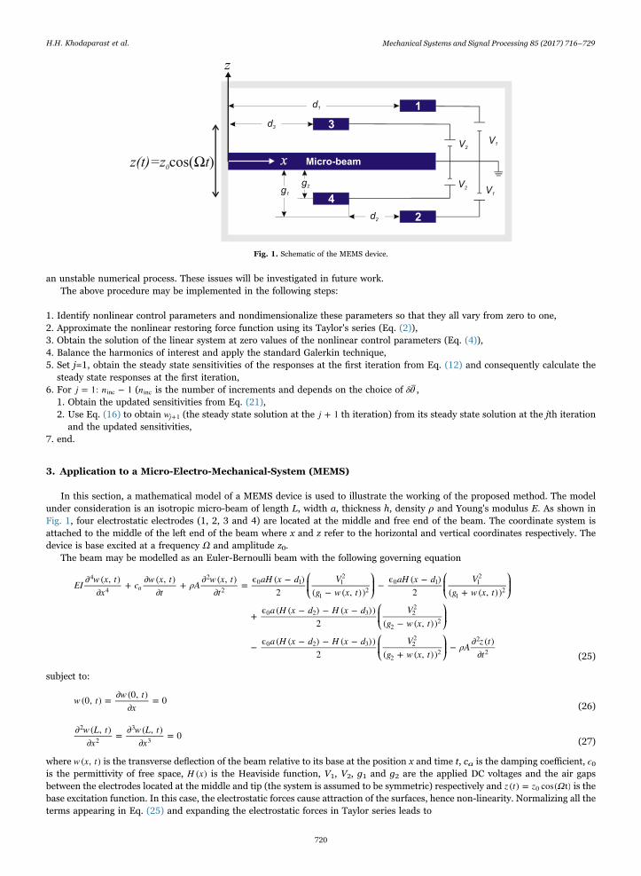
In this section, a mathematical model of a MEMS device is used to illustrate the working of the proposed method. The modelunder consideration is an isotropic micro-beam of length L, width a, thickness h, density ρ and Young's modulus E. As shown inFig. 1, four electrostatic electrodes (1, 2, 3 and 4) are located at the middle and free end of the beam. The coordinate system isattached to the middle of the left end of the beam where x and z refer to the horizontal and vertical coordinates respectively. Thedevice is base excited at a frequency Ω and amplitude z0.
The beam may be modelled as an Euler-Bernoulli beam with the following governing equation
EI w x tx
c w x tt
ρA w x tt
aH x d Vg w x t
aH x d Vg w x t
a H x d H x d Vg w x t
a H x d H x d Vg w x t
ρA z tt
∂ ( , )∂
+ ∂ ( , )∂
+ ∂ ( , )∂
= ϵ ( − )2 ( − ( , ))
− ϵ ( − )2 ( + ( , ))
+ ϵ ( ( − ) − ( − ))2 ( − ( , ))
− ϵ ( ( − ) − ( − ))2 ( + ( , ))
− ∂ ( )∂
a4
4
2
20 1 1
2
12
0 1 12
12
0 2 3 22
22
0 2 3 22
22
2
2
⎛⎝⎜
⎞⎠⎟
⎛⎝⎜
⎞⎠⎟
⎛⎝⎜
⎞⎠⎟
⎛⎝⎜
⎞⎠⎟ (25)
subject to:
w t w tx
(0, ) = ∂ (0, )∂
= 0(26)
w L tx
w L tx
∂ ( , )∂
= ∂ ( , )∂
= 02
2
3
3 (27)
where w x t( , ) is the transverse deflection of the beam relative to its base at the position x and time t, ca is the damping coefficient, ϵ0is the permittivity of free space, H x( ) is the Heaviside function, V1, V2, g1 and g2 are the applied DC voltages and the air gapsbetween the electrodes located at the middle and tip (the system is assumed to be symmetric) respectively and z t z Ω( ) = cos( t)0 is thebase excitation function. In this case, the electrostatic forces cause attraction of the surfaces, hence non-linearity. Normalizing all theterms appearing in Eq. (25) and expanding the electrostatic forces in Taylor series leads to
Fig. 1. Schematic of the MEMS device.
H.H. Khodaparast et al. Mechanical Systems and Signal Processing 85 (2017) 716–729
720
w x tx
c w x tt
w x t
tα w α w w γ iΩ t cc∂ ( , ^)
∂+ ∂ ( , ^)
∂^ + ∂ ( , ^)∂^
+ + + ( ) = exp( ^) + .4
4
2
2 1 33 5
(28)
where
w w g x x L t t T Ω ΩT λgg
c c LEIT
T ρALEI
η aLEIg
γ z ρAL ΩEIg
α ηV θ H x d LηV θ H x d L H x d L
λ
α ηV θ H x d LηV θ H x d L H x d L
λ
= / 1, = / , ^ = / , = , = ,
= , = , = ϵ , =2
,
= −2 ( − / ) +( ( − / ) − ( − / ))
= −4 ( − / ) +( ( − / ) − ( − / ))
a
2
1
4 40
4
13
04 2
1
1 012
12
1022
22
2 33
3 012
12
1022
22
2 35
⎛⎝⎜
⎞⎠⎟
⎛⎝⎜
⎞⎠⎟
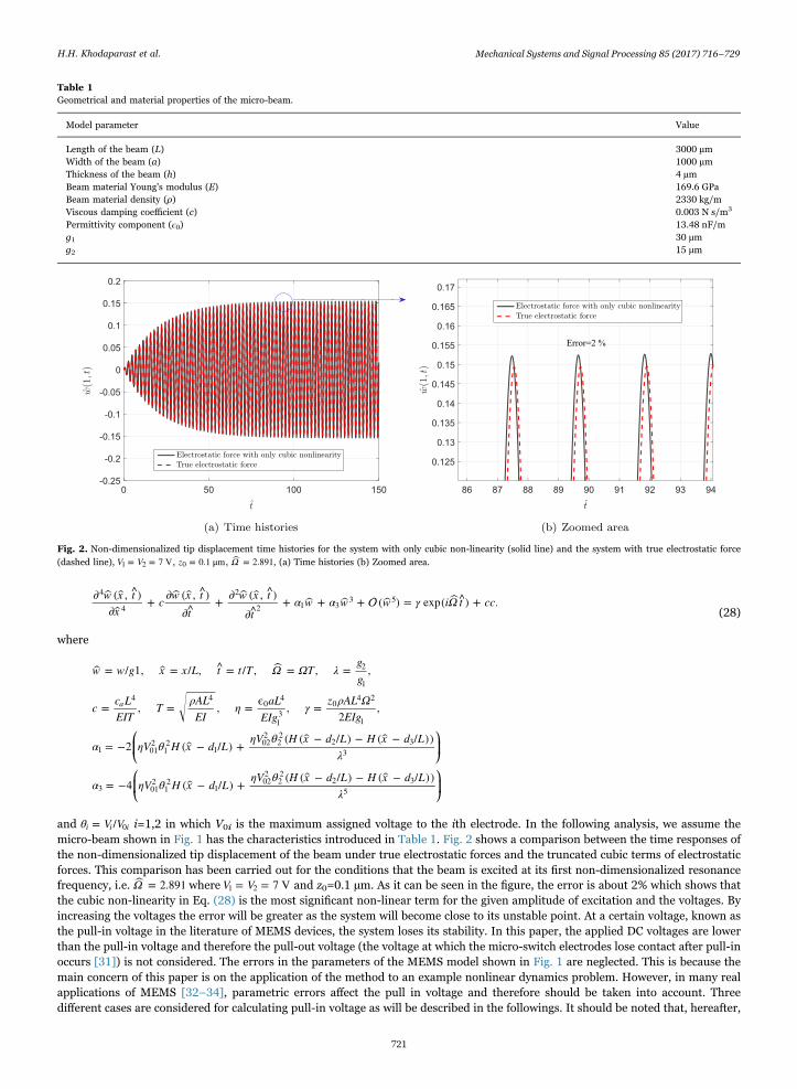
and θ V V= /i i i0 i=1,2 in which V0i is the maximum assigned voltage to the ith electrode. In the following analysis, we assume themicro-beam shown in Fig. 1 has the characteristics introduced in Table 1. Fig. 2 shows a comparison between the time responses ofthe non-dimensionalized tip displacement of the beam under true electrostatic forces and the truncated cubic terms of electrostaticforces. This comparison has been carried out for the conditions that the beam is excited at its first non-dimensionalized resonancefrequency, i.e. Ω = 2.891 where V V= = 7 V1 2 and z0=0.1 µm. As it can be seen in the figure, the error is about 2% which shows thatthe cubic non-linearity in Eq. (28) is the most significant non-linear term for the given amplitude of excitation and the voltages. Byincreasing the voltages the error will be greater as the system will become close to its unstable point. At a certain voltage, known asthe pull-in voltage in the literature of MEMS devices, the system loses its stability. In this paper, the applied DC voltages are lowerthan the pull-in voltage and therefore the pull-out voltage (the voltage at which the micro-switch electrodes lose contact after pull-inoccurs [31]) is not considered. The errors in the parameters of the MEMS model shown in Fig. 1 are neglected. This is because themain concern of this paper is on the application of the method to an example nonlinear dynamics problem. However, in many realapplications of MEMS [32–34], parametric errors affect the pull in voltage and therefore should be taken into account. Threedifferent cases are considered for calculating pull-in voltage as will be described in the followings. It should be noted that, hereafter,
Table 1Geometrical and material properties of the micro-beam.
Model parameter Value
Length of the beam (L) 3000 µmWidth of the beam (a) 1000 µmThickness of the beam (h) 4 µmBeam material Young's modulus (E) 169.6 GPaBeam material density (ρ) 2330 kg/mViscous damping coefficient (c) 0.003 N s/m3
Fig. 2. Non-dimensionalized tip displacement time histories for the system with only cubic non-linearity (solid line) and the system with true electrostatic force(dashed line), V V= = 7 V1 2 , z = 0.1 μm0 , Ω = 2.891, (a) Time histories (b) Zoomed area.
H.H. Khodaparast et al. Mechanical Systems and Signal Processing 85 (2017) 716–729
721
the effects of the 5th and higher order terms of electrostatic forces are ignored.The method described in Section 2 is now illustrated in the above example of a micro-beam with nonlinear electrostatic force.
Comparing Eq. (28) to Eqs. (1) and (2), we have k=1, ρ = 1, Γ ≡x
∂∂
4
4 , f γ= 2 and x x= { ∈ : 0 ≤ ≤ 1}. The first two modes of thebeam are considered for the analysis, hence N=2. The mode shapes of a clamped-free beam having unit length are
where β = 1.875104071 and β = 4.694091132 . Knowing that the system has only cubic non-linearity (H=3) and assuming the primaryharmonic responses only (L=1), A ∈1
2×2, b ∈12, A ∈j
2×2 and b ∈j2 can be calculated according to Eqs. (13), (15), (22) and
(24) respectively. In this example, the nonlinear control parameters are assumed as θ V V= /1 1 01 and θ V V= /2 2 02 where V01 and V02 arethe maximum voltages that can be applied to the system. Three different case studies are considered in this section. The first case iswhen all electrodes are included in the circuit, while in the second case electrodes 3 and 4 are disconnected from the circuit, henceθ = 02 and finally electrodes 1 and 2 will be removed in the third case in which θ = 01 . In case 1 the solutions obtained by theproposed method are validated using numerical integration results.
3.1. Case 1
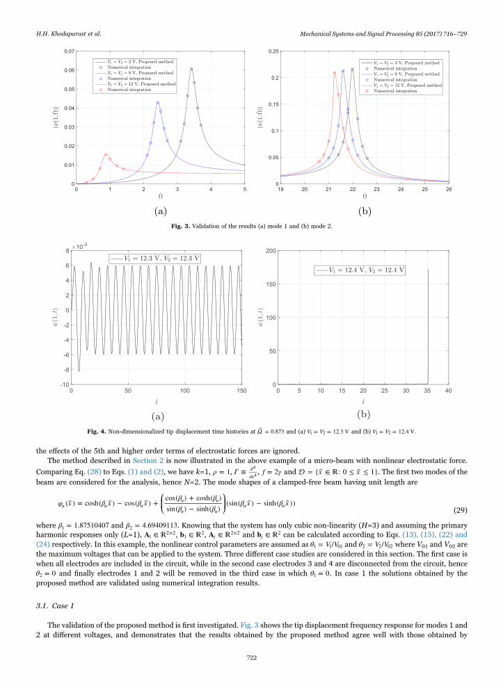
The validation of the proposed method is first investigated. Fig. 3 shows the tip displacement frequency response for modes 1 and2 at different voltages, and demonstrates that the results obtained by the proposed method agree well with those obtained by
Fig. 3. Validation of the results (a) mode 1 and (b) mode 2.
Fig. 4. Non-dimensionalized tip displacement time histories at Ω = 0.873 and (a) V V= = 12.3 V1 2 and (b) V V= = 12.4 V1 2 .
H.H. Khodaparast et al. Mechanical Systems and Signal Processing 85 (2017) 716–729
722
numerical integration. The results also showed that the proposed method is capable of predicting the frequency response of anonlinear system with a strong but smooth non-linearity (high voltages).
To calculate the pull-in voltage in this case, both V1 and V2 are gradually and equally increased at different frequencies and thesolution is sought using numerical integration. This is shown in Fig. 4 where the beam tip displacement time histories atV V= = 12.3 V1 2 and V V= = 12.4 V1 2 are shown. As can be seen in the figure, the displacement grows unboundedly onceV V= = 12.4 V1 2 . Therefore the analysis is carried out for voltages between 0 and 12 V in this case.
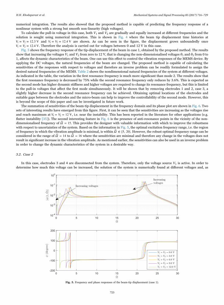
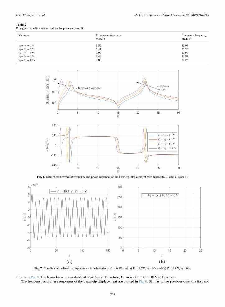
Fig. 5 shows the frequency response of the tip-displacement of the beam in case 1, obtained by the proposed method. The resultsshow that increasing the voltages V1 and V2 from zero to 12 V, that is changing the non-dimensionalised voltages θ1 and θ2 from 0 to1, affects the dynamic characteristics of the beam. One can use this effect to control the vibration responses of the MEMS device. Byapplying the DC voltages, the natural frequencies of the beam are changed. The proposed method is capable of calculating thesensitivities of the responses with respect to voltages and therefore an inverse problem can be readily formulated to assign thedesired natural frequencies of the MEMS. Table 2 shows the nondimensional natural frequencies of the system at different voltages.As indicated in the table, the variation in the first resonance frequency is much more significant than mode 2. The results show thatthe first resonance frequency is decreased by 75% while the second resonance frequency only reduces by 3.6%. This is expected asthe second mode has higher dynamic stiffness and higher voltages are required to change its resonance frequency, but this is limitedto the pull-in voltages that affect the first mode simultaneously. It will be shown that by removing electrodes 1 and 2, case 3, aslightly higher decrease in the second resonance frequency can be achieved. Obtaining optimal locations of the electrodes andsuitable gaps between the electrodes and the micro-beam can help to improve the controllability of the second mode. However, thisis beyond the scope of this paper and can be investigated in future work.
The summation of sensitivities of the beam-tip displacement in the frequency domain and its phase plot are shown in Fig. 6. Twosets of interesting results have emerged from this figure. First, it can be seen that the sensitivities are increasing as the voltages riseand reach maximum at V V= = 12 V1 2 , i.e. near the instability. This has been reported in the literature for other applications (e.g.flutter instability [35]). The second interesting feature in Fig. 6 is the presence of anti-resonance points in the vicinity of the non-dimensionalised frequency of Ω = 15. This provides the designer with valuable information with which to improve the robustnesswith respect to uncertainties of the system. Based on the information in Fig. 5, the optimal excitation frequency range, i.e. the regionof frequency in which the vibration amplitude is minimal, is within Ω ∈ [5, 20]. However, the robust optimal frequency range can beconsidered in the range of Ω = 14 to Ω = 16 where the sensitivities are minimal and therefore any change in the voltages does notresult in significant increase in the vibration amplitude. As mentioned earlier, the sensitivities can also be used in an inverse problemin order to change the dynamic characteristics of the system in a desirable way.
3.2. Case 2
In this case, electrodes 3 and 4 are disconnected from the system. Therefore, only the voltage source V1 is active. In order todetermine how much this voltage can be increased, the solution of the system is numerically found at different voltages and, as
Fig. 5. Frequency and phase responses of the beam-tip displacement (case 1).
H.H. Khodaparast et al. Mechanical Systems and Signal Processing 85 (2017) 716–729
723
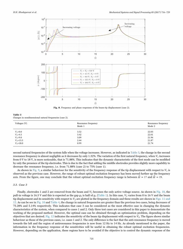
shown in Fig. 7, the beam becomes unstable at V1=18.8 V. Therefore, V1 varies from 0 to 18 V in this case.The frequency and phase responses of the beam-tip displacement are plotted in Fig. 8. Similar to the previous case, the first and
Table 2Changes in nondimensional natural frequencies (case 1).
Voltages Resonance frequency Resonance frequencyMode 1 Mode 2
Fig. 6. Sum of sensitivities of frequency and phase responses of the beam-tip displacement with respect to V1 and V2 (case 1).
Fig. 7. Non-dimensionalized tip displacement time histories at Ω = 0.873 and (a) V1=18.7 V, V = 0 V2 and (b) V1=18.8 V, V = 0 V2 .
H.H. Khodaparast et al. Mechanical Systems and Signal Processing 85 (2017) 716–729
724
second natural frequencies of the system falls when the voltage increases. However, as indicated in Table 3, the change in the secondresonance frequency is almost negligible as it decreases by only 1.32%. The variation of the first natural frequency, when V1 increasesfrom 0 V to 18 V, is more noticeable, that is 71.88%. This indicates that the dynamic characteristic of the first mode can be modifiedby only the presence of the tip electrodes. This is due to the fact that adding the middle electrodes provides slightly more capability todecrease the resonance frequency, i.e. from 71.88% (case 2) to 75% (case 1).
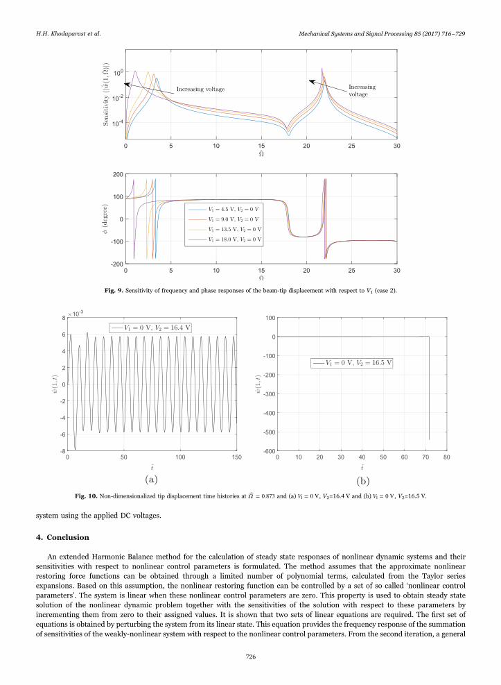
As shown in Fig. 9, a similar behaviour for the sensitivity of the frequency response of the tip displacement with respect to V1 isobserved as the previous case. However, the range of robust optimal excitation frequency has been moved further up the frequencyaxis. From the figure, one may conclude that the robust optimal excitation frequency range is between Ω = 17 and Ω = 19.
3.3. Case 3
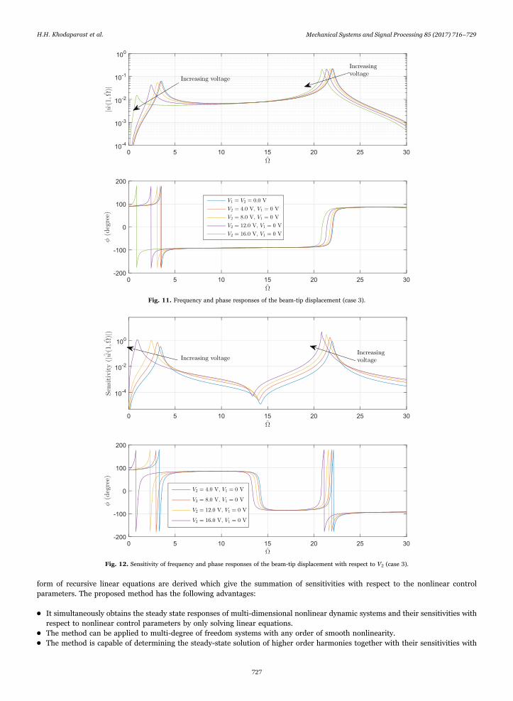
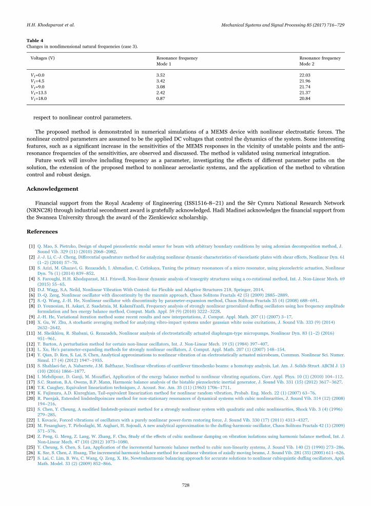
Finally, electrodes 1 and 2 are removed from the beam and V2 becomes the only active voltage source. As shown in Fig. 10, thepull-in voltage is 16.5 V and this is expected as the gap g2 is half of g1 (Table 1). In this case, V2 varies from 0 to 16 V and the beamtip displacement and its sensitivity with respect to V2 are plotted in the frequency domain and these results are shown in Figs. 11 and12. As can be see in Fig. 10 and Table 4, the change in natural frequencies are greater than the previous two cases, being decreases of75.28% and 5.14% respectively. This indicates that case 3 can be considered as the most effective case in changing the dynamiccharacteristics of the system, when compared to cases 1 and 2. Only three test cases are considered in this paper to demonstrate theworking of the proposed method. However, the optimal case can be obtained through an optimization problem, depending on theobjectives that are desired. Fig. 12 indicates the sensitivity of the beam tip displacement with respect to V2. The figure shows similarbehaviour as those of the previous cases, i.e. cases 1 and 2. The only difference is the fact that the anti-resonance frequency is movedtowards the left and the region of antiresonance frequencies is now from 12 Hz to 14 Hz. As already mentioned in the paper, theinformation in the frequency response of the sensitivities will be useful in obtaining the robust optimal excitation frequencies.However, depending on the application, these regions have to be avoided if the objective is to control the dynamic response of the
Fig. 8. Frequency and phase responses of the beam-tip displacement (case 2).
Table 3Changes in nondimensional natural frequencies (case 2).
Voltages (V) Resonance frequency Resonance frequencyMode 1 Mode 2
H.H. Khodaparast et al. Mechanical Systems and Signal Processing 85 (2017) 716–729
725
system using the applied DC voltages.
4. Conclusion
An extended Harmonic Balance method for the calculation of steady state responses of nonlinear dynamic systems and theirsensitivities with respect to nonlinear control parameters is formulated. The method assumes that the approximate nonlinearrestoring force functions can be obtained through a limited number of polynomial terms, calculated from the Taylor seriesexpansions. Based on this assumption, the nonlinear restoring function can be controlled by a set of so called ‘nonlinear controlparameters’. The system is linear when these nonlinear control parameters are zero. This property is used to obtain steady statesolution of the nonlinear dynamic problem together with the sensitivities of the solution with respect to these parameters byincrementing them from zero to their assigned values. It is shown that two sets of linear equations are required. The first set ofequations is obtained by perturbing the system from its linear state. This equation provides the frequency response of the summationof sensitivities of the weakly-nonlinear system with respect to the nonlinear control parameters. From the second iteration, a general
Fig. 9. Sensitivity of frequency and phase responses of the beam-tip displacement with respect to V1 (case 2).
Fig. 10. Non-dimensionalized tip displacement time histories at Ω = 0.873 and (a) V = 0 V1 , V2=16.4 V and (b) V = 0 V1 , V2=16.5 V.
H.H. Khodaparast et al. Mechanical Systems and Signal Processing 85 (2017) 716–729
726
form of recursive linear equations are derived which give the summation of sensitivities with respect to the nonlinear controlparameters. The proposed method has the following advantages:
• It simultaneously obtains the steady state responses of multi-dimensional nonlinear dynamic systems and their sensitivities withrespect to nonlinear control parameters by only solving linear equations.
• The method can be applied to multi-degree of freedom systems with any order of smooth nonlinearity.
• The method is capable of determining the steady-state solution of higher order harmonies together with their sensitivities with
Fig. 11. Frequency and phase responses of the beam-tip displacement (case 3).
Fig. 12. Sensitivity of frequency and phase responses of the beam-tip displacement with respect to V2 (case 3).
H.H. Khodaparast et al. Mechanical Systems and Signal Processing 85 (2017) 716–729
727
respect to nonlinear control parameters.
The proposed method is demonstrated in numerical simulations of a MEMS device with nonlinear electrostatic forces. Thenonlinear control parameters are assumed to be the applied DC voltages that control the dynamics of the system. Some interestingfeatures, such as a significant increase in the sensitivities of the MEMS responses in the vicinity of unstable points and the anti-resonance frequencies of the sensitivities, are observed and discussed. The method is validated using numerical integration.
Future work will involve including frequency as a parameter, investigating the effects of different parameter paths on thesolution, the extension of the proposed method to nonlinear aeroelastic systems, and the application of the method to vibrationcontrol and robust design.
Acknowledgement
Financial support from the Royal Academy of Engineering (ISS1516-8–21) and the Sêr Cymru National Research Network(NRNC28) through industrial secondment award is gratefully acknowledged. Hadi Madinei acknowledges the financial support fromthe Swansea University through the award of the Zienkiewicz scholarship.
References
[1] Q. Mao, S. Pietrzko, Design of shaped piezoelectric modal sensor for beam with arbitrary boundary conditions by using adomian decomposition method, J.Sound Vib. 329 (11) (2010) 2068–2082.
[2] J.-J. Li, C.-J. Cheng, Differential quadrature method for analyzing nonlinear dynamic characteristics of viscoelastic plates with shear effects, Nonlinear Dyn. 61(1–2) (2010) 57–70.
[3] S. Azizi, M. Ghazavi, G. Rezazadeh, I. Ahmadian, C. Cetinkaya, Tuning the primary resonances of a micro resonator, using piezoelectric actuation, NonlinearDyn. 76 (1) (2014) 839–852.
[4] S. Faroughi, H.H. Khodaparast, M.I. Friswell, Non-linear dynamic analysis of tensegrity structures using a co-rotational method, Int. J. Non-Linear Mech. 69(2015) 55–65.
[5] D.J. Wagg, S.A. Neild, Nonlinear Vibration With Control: for Flexible and Adaptive Structures 218, Springer, 2014.[6] D.-Q. Zeng, Nonlinear oscillator with discontinuity by the maxmin approach, Chaos Solitons Fractals 42 (5) (2009) 2885–2889.[7] S.-Q. Wang, J.-H. He, Nonlinear oscillator with discontinuity by parameter-expansion method, Chaos Solitons Fractals 35 (4) (2008) 688–691.[8] D. Younesian, H. Askari, Z. Saadatnia, M. KalamiYazdi, Frequency analysis of strongly nonlinear generalized duffing oscillators using hes frequency amplitude
formulation and hes energy balance method, Comput. Math. Appl. 59 (9) (2010) 3222–3228.[9] J.-H. He, Variational iteration method some recent results and new interpretations, J. Comput. Appl. Math. 207 (1) (2007) 3–17.
[10] X. Gu, W. Zhu, A stochastic averaging method for analyzing vibro-impact systems under gaussian white noise excitations, J. Sound Vib. 333 (9) (2014)2632–2642.
[11] M. Sheikhlou, R. Shabani, G. Rezazadeh, Nonlinear analysis of electrostatically actuated diaphragm-type micropumps, Nonlinear Dyn. 83 (1–2) (2016)951–961.
[12] T. Burton, A perturbation method for certain non-linear oscillators, Int. J. Non-Linear Mech. 19 (5) (1984) 397–407.[13] L. Xu, He's parameter-expanding methods for strongly nonlinear oscillators, J. Comput. Appl. Math. 207 (1) (2007) 148–154.[14] Y. Qian, D. Ren, S. Lai, S. Chen, Analytical approximations to nonlinear vibration of an electrostatically actuated microbeam, Commun. Nonlinear Sci. Numer.
Simul. 17 (4) (2012) 1947–1955.[15] S. Shahlaei-far, A. Nabarrete, J.M. Balthazar, Nonlinear vibrations of cantilever timoshenko beams: a homotopy analysis, Lat. Am. J. Solids Struct. ABCM J. 13
(10) (2016) 1866–1877.[16] I. Mehdipour, D. Ganji, M. Mozaffari, Application of the energy balance method to nonlinear vibrating equations, Curr. Appl. Phys. 10 (1) (2010) 104–112.[17] S.C. Stanton, B.A. Owens, B.P. Mann, Harmonic balance analysis of the bistable piezoelectric inertial generator, J. Sound Vib. 331 (15) (2012) 3617–3627.[18] T.K. Caughey, Equivalent linearization techniques, J. Acoust. Soc. Am. 35 (11) (1963) 1706–1711.[19] K. Fujimura, A.D. Kiureghian, Tail-equivalent linearization method for nonlinear random vibration, Probab. Eng. Mech. 22 (1) (2007) 63–76.[20] R. Puenjak, Extended lindstedtpoincare method for non-stationary resonances of dynamical systems with cubic nonlinearities, J. Sound Vib. 314 (12) (2008)
194–216.[21] S. Chen, Y. Cheung, A modified lindstedt-poincaré method for a strongly nonlinear system with quadratic and cubic nonlinearities, Shock Vib. 3 (4) (1996)
279–285.[22] I. Kovacic, Forced vibrations of oscillators with a purely nonlinear power-form restoring force, J. Sound Vib. 330 (17) (2011) 4313–4327.[23] M. Fesanghary, T. Pirbodaghi, M. Asghari, H. Sojoudi, A new analytical approximation to the duffing-harmonic oscillator, Chaos Solitons Fractals 42 (1) (2009)
571–576.[24] Z. Peng, G. Meng, Z. Lang, W. Zhang, F. Chu, Study of the effects of cubic nonlinear damping on vibration isolations using harmonic balance method, Int. J.
Non-Linear Mech. 47 (10) (2012) 1073–1080.[25] Y. Cheung, S. Chen, S. Lau, Application of the incremental harmonic balance method to cubic non-linearity systems, J. Sound Vib. 140 (2) (1990) 273–286.[26] K. Sze, S. Chen, J. Huang, The incremental harmonic balance method for nonlinear vibration of axially moving beams, J. Sound Vib. 281 (35) (2005) 611–626.[27] S. Lai, C. Lim, B. Wu, C. Wang, Q. Zeng, X. He, Newtonharmonic balancing approach for accurate solutions to nonlinear cubicquintic duffing oscillators, Appl.
Math. Model. 33 (2) (2009) 852–866.
Table 4Changes in nondimensional natural frequencies (case 3).
Voltages (V) Resonance frequency Resonance frequencyMode 1 Mode 2
[28] A. Grolet, F. Thouverez, On a new harmonic selection technique for harmonic balance method, Mech. Syst. Signal Process. 30 (2012) 43–60.[29] Z. Guo, X. Ma, Residue harmonic balance solution procedure to nonlinear delay differential systems, Appl. Math. Comput. 237 (2014) 20–30.[30] P. Ju, X. Xue, Global residue harmonic balance method to periodic solutions of a class of strongly nonlinear oscillators, Appl. Math. Model. 38 (24) (2014)
6144–6152.[31] H. Samaali, F. Najar, S. Choura, A.H. Nayfeh, M. Masmoudi, A double microbeam mems ohmic switch for rf-applications with low actuation voltage, Nonlinear
Dyn. 63 (4) (2011) 719–734.[32] J.M. Balthazar, D.G. Bassinello, A.M. Tusset, Á.M. Bueno, B.R. de Pontes Junior, Nonlinear control in an electromechanical transducer with chaotic behaviour,
Meccanica 49 (8) (2014) 1859–1867.[33] N. Peruzzi, F. Chavarette, J. Balthazar, A. Tusset, A. Perticarrari, R. Brasil, The dynamic behavior of a parametrically excited time-periodic mems taking into
account parametric errors, J. Vib. Control. ⟨http://dx.doi.org/10.1177/1077546315573913⟩.[34] A.M. Tusset, J.M. Balthazar, D.G. Bassinello, B.R. Pontes, J.L.P. Felix, Statements on chaos control designs, including a fractional order dynamical system,
applied to a “mems” comb-drive actuator, Nonlinear Dyn. 69 (4) (2012) 1837–1857.[35] H.H. Khodaparast, J.E. Mottershead, K.J. Badcock, Propagation of structural uncertainty to linear aeroelastic stability, Comput. Struct. 88 (3–4) (2010)
223–236.
H.H. Khodaparast et al. Mechanical Systems and Signal Processing 85 (2017) 716–729


![A globally convergent incremental Newton method...Incremental Newton 3 extended Kalman lter (EKF) method with variable stepsize or equivalently the EKF-S algorithm [20], and shows](https://static.documents.pub/doc/80x56/607645be86b0bf621f2f18ba/a-globally-convergent-incremental-newton-method-incremental-newton-3-extended.jpg)


