An Introduction to Veterinary Epidemiology...8 An Introduction to Veterinary Epidemiology In...

An Introduction to Veterinary Epidemiology

Mark Stevenson

EpiCentre, IVABS

Massey University, Palmerston North, New Zealand

Contributions from Dirk Pfeiffer, Nigel Perkins, and John Morton are grate-fully acknowledged.

EpiCentre, IVABS, Massey UniversityPrivate Bag 11-222 Palmerston NorthNew Zealand October, 2004

2 An Introduction to Veterinary Epidemiology

Contents

1 Introduction 71.1 Host, agent, and environment . . . . . . . . . . . . . . . . . . . . . . . . 81.2 Individual, place, and time . . . . . . . . . . . . . . . . . . . . . . . . . . 8

1.2.1 Individual . . . . . . . . . . . . . . . . . . . . . . . . . . . . . . . 91.2.2 Place . . . . . . . . . . . . . . . . . . . . . . . . . . . . . . . . . . 91.2.3 Time . . . . . . . . . . . . . . . . . . . . . . . . . . . . . . . . . . 10

1.3 Causation . . . . . . . . . . . . . . . . . . . . . . . . . . . . . . . . . . . 121.4 Historical examples in the development of epidemiology . . . . . . . . . . 14

1.4.1 Ignas Semmelweis . . . . . . . . . . . . . . . . . . . . . . . . . . . 141.4.2 John Snow . . . . . . . . . . . . . . . . . . . . . . . . . . . . . . . 15

2 Measures of health 162.1 Prevalence . . . . . . . . . . . . . . . . . . . . . . . . . . . . . . . . . . . 162.2 Incidence . . . . . . . . . . . . . . . . . . . . . . . . . . . . . . . . . . . . 17

2.2.1 Incidence risk . . . . . . . . . . . . . . . . . . . . . . . . . . . . . 172.2.2 Incidence rate . . . . . . . . . . . . . . . . . . . . . . . . . . . . . 18

2.3 Comparison of prevalence and incidence . . . . . . . . . . . . . . . . . . 202.4 Conversions . . . . . . . . . . . . . . . . . . . . . . . . . . . . . . . . . . 202.5 Other measures of disease frequency . . . . . . . . . . . . . . . . . . . . . 21

2.5.1 Attack rates . . . . . . . . . . . . . . . . . . . . . . . . . . . . . . 212.5.2 Secondary attack rates . . . . . . . . . . . . . . . . . . . . . . . . 222.5.3 Mortality . . . . . . . . . . . . . . . . . . . . . . . . . . . . . . . 222.5.4 Case fatality rate . . . . . . . . . . . . . . . . . . . . . . . . . . . 222.5.5 Proportional mortality . . . . . . . . . . . . . . . . . . . . . . . . 22

2.6 Adjusted rates . . . . . . . . . . . . . . . . . . . . . . . . . . . . . . . . . 222.6.1 Stratum-specific rates . . . . . . . . . . . . . . . . . . . . . . . . . 232.6.2 Comparing rates . . . . . . . . . . . . . . . . . . . . . . . . . . . 232.6.3 Unstable rates due to small numbers . . . . . . . . . . . . . . . . 242.6.4 Direct adjustment . . . . . . . . . . . . . . . . . . . . . . . . . . . 242.6.5 Indirect adjustment . . . . . . . . . . . . . . . . . . . . . . . . . . 25

3 Study design 283.1 Descriptive studies . . . . . . . . . . . . . . . . . . . . . . . . . . . . . . 29

3.1.1 Case reports . . . . . . . . . . . . . . . . . . . . . . . . . . . . . . 293.1.2 Cases series . . . . . . . . . . . . . . . . . . . . . . . . . . . . . . 293.1.3 Descriptive studies based on rates . . . . . . . . . . . . . . . . . . 29

3.2 Analytical studies . . . . . . . . . . . . . . . . . . . . . . . . . . . . . . . 303.2.1 Randomised clinical trials . . . . . . . . . . . . . . . . . . . . . . 303.2.2 Cohort studies . . . . . . . . . . . . . . . . . . . . . . . . . . . . . 313.2.3 Case-control studies . . . . . . . . . . . . . . . . . . . . . . . . . . 323.2.4 Cross-sectional studies . . . . . . . . . . . . . . . . . . . . . . . . 33

3.3 A comparison of cohort, case-control and cross-sectional study designs . . 34

M. Stevenson 3

3.4 Errors in study design . . . . . . . . . . . . . . . . . . . . . . . . . . . . 35

4 Measures of association 374.1 Measures of strength . . . . . . . . . . . . . . . . . . . . . . . . . . . . . 38

4.1.1 Risk ratio . . . . . . . . . . . . . . . . . . . . . . . . . . . . . . . 384.1.2 Incidence rate ratio . . . . . . . . . . . . . . . . . . . . . . . . . . 384.1.3 Odds ratio . . . . . . . . . . . . . . . . . . . . . . . . . . . . . . . 39

4.2 Measures of effect in the exposed population . . . . . . . . . . . . . . . . 394.2.1 Attributable rate (rate) . . . . . . . . . . . . . . . . . . . . . . . . 394.2.2 Attributable fraction . . . . . . . . . . . . . . . . . . . . . . . . . 39

4.3 Measures of effect in the total population . . . . . . . . . . . . . . . . . . 404.3.1 Population attributable risk (rate) . . . . . . . . . . . . . . . . . . 404.3.2 Population attributable fraction . . . . . . . . . . . . . . . . . . . 40

4.4 Using the appropriate measure of effect . . . . . . . . . . . . . . . . . . . 41

5 Statistical inference 435.1 Statistical significance and confidence intervals . . . . . . . . . . . . . . . 445.2 Steps involved in testing significance . . . . . . . . . . . . . . . . . . . . 44

6 Diagnostic tests 476.1 Screening versus diagnosis . . . . . . . . . . . . . . . . . . . . . . . . . . 476.2 Sensitivity and specificity . . . . . . . . . . . . . . . . . . . . . . . . . . . 486.3 Accuracy and precision . . . . . . . . . . . . . . . . . . . . . . . . . . . . 48

6.3.1 Measuring accuracy . . . . . . . . . . . . . . . . . . . . . . . . . . 496.3.2 Measuring precision . . . . . . . . . . . . . . . . . . . . . . . . . . 49

6.4 Test evaluation . . . . . . . . . . . . . . . . . . . . . . . . . . . . . . . . 496.4.1 The gold standard . . . . . . . . . . . . . . . . . . . . . . . . . . 496.4.2 Sensitivity . . . . . . . . . . . . . . . . . . . . . . . . . . . . . . . 506.4.3 Specificity . . . . . . . . . . . . . . . . . . . . . . . . . . . . . . . 506.4.4 Positive predictive value . . . . . . . . . . . . . . . . . . . . . . . 516.4.5 Negative predictive value . . . . . . . . . . . . . . . . . . . . . . . 51

6.5 Prevalence estimation . . . . . . . . . . . . . . . . . . . . . . . . . . . . . 526.6 Diagnostic strategies . . . . . . . . . . . . . . . . . . . . . . . . . . . . . 53

6.6.1 Parallel interpretation . . . . . . . . . . . . . . . . . . . . . . . . 546.6.2 Serial interpretation . . . . . . . . . . . . . . . . . . . . . . . . . 546.6.3 Screening and confirmatory testing . . . . . . . . . . . . . . . . . 546.6.4 Batteries of multiple tests . . . . . . . . . . . . . . . . . . . . . . 556.6.5 Likelihood ratios . . . . . . . . . . . . . . . . . . . . . . . . . . . 55

7 Sampling populations 597.1 Probability sampling methods . . . . . . . . . . . . . . . . . . . . . . . . 59

7.1.1 Simple random sampling . . . . . . . . . . . . . . . . . . . . . . . 597.1.2 Systematic random sampling . . . . . . . . . . . . . . . . . . . . . 607.1.3 Stratified random sampling . . . . . . . . . . . . . . . . . . . . . 60


7.1.4 Cluster sampling . . . . . . . . . . . . . . . . . . . . . . . . . . . 617.2 Non-probability sampling . . . . . . . . . . . . . . . . . . . . . . . . . . . 627.3 Sources of error in sample estimates and how to reduce error . . . . . . . 63

7.3.1 Random error . . . . . . . . . . . . . . . . . . . . . . . . . . . . . 637.3.2 Bias . . . . . . . . . . . . . . . . . . . . . . . . . . . . . . . . . . 63

7.4 Common sampling methods . . . . . . . . . . . . . . . . . . . . . . . . . 647.4.1 Methods of randomisation . . . . . . . . . . . . . . . . . . . . . . 647.4.2 Replacement . . . . . . . . . . . . . . . . . . . . . . . . . . . . . . 64

7.5 Taking a sample of the appropriate size . . . . . . . . . . . . . . . . . . . 657.5.1 Simple random sampling . . . . . . . . . . . . . . . . . . . . . . . 657.5.2 Proving freedom from disease . . . . . . . . . . . . . . . . . . . . 66

7.6 Estimation of the proportion of diseased animals in a population . . . . . 66

8 Outbreak investigation 688.1 Verify the outbreak . . . . . . . . . . . . . . . . . . . . . . . . . . . . . . 68

8.1.1 What is the illness? . . . . . . . . . . . . . . . . . . . . . . . . . . 688.1.2 Is there a true excess of disease? . . . . . . . . . . . . . . . . . . . 68

8.2 Investigating an outbreak . . . . . . . . . . . . . . . . . . . . . . . . . . 698.2.1 Establish a case definition . . . . . . . . . . . . . . . . . . . . . . 698.2.2 Enhance surveillance . . . . . . . . . . . . . . . . . . . . . . . . . 698.2.3 Describe outbreak according to individual, place and time . . . . 698.2.4 Develop hypotheses about the nature of exposure . . . . . . . . . 708.2.5 Conduct analytical studies . . . . . . . . . . . . . . . . . . . . . . 70

8.3 Implement disease control interventions . . . . . . . . . . . . . . . . . . . 70

9 Appraising the literature 719.1 Description of the evidence . . . . . . . . . . . . . . . . . . . . . . . . . . 719.2 Internal validity - non-causal explanations . . . . . . . . . . . . . . . . . 729.3 Internal validity - positive features of causation . . . . . . . . . . . . . . 72

9.3.1 Is there a correct temporal relationship? . . . . . . . . . . . . . . 729.3.2 Is the relationship strong? . . . . . . . . . . . . . . . . . . . . . . 729.3.3 Is there a dose-response relationship? . . . . . . . . . . . . . . . . 739.3.4 Consistency of the association . . . . . . . . . . . . . . . . . . . . 739.3.5 Specificity of association . . . . . . . . . . . . . . . . . . . . . . . 73

9.4 External validity - generalisation of the results . . . . . . . . . . . . . . . 739.4.1 Can the results be applied to the eligible population? . . . . . . . 749.4.2 Can the results be applied to the source population? . . . . . . . 749.4.3 Can the results be applied to other relevant populations? . . . . . 74

9.5 Comparison of the results with other evidence . . . . . . . . . . . . . . . 749.5.1 Are the results consistent with other evidence? . . . . . . . . . . . 759.5.2 Does the total evidence suggest any specificity? . . . . . . . . . . 759.5.3 Are the results plausible biologically? . . . . . . . . . . . . . . . . 759.5.4 Coherency with the distribution of the exposure and the outcome? 75

M. Stevenson 5

10 Exercise: outbreak investigation 7710.1 The problem . . . . . . . . . . . . . . . . . . . . . . . . . . . . . . . . . . 7710.2 Question 1 . . . . . . . . . . . . . . . . . . . . . . . . . . . . . . . . . . . 7710.3 Question 2 . . . . . . . . . . . . . . . . . . . . . . . . . . . . . . . . . . . 7810.4 Question 3 . . . . . . . . . . . . . . . . . . . . . . . . . . . . . . . . . . . 7910.5 Question 4 . . . . . . . . . . . . . . . . . . . . . . . . . . . . . . . . . . . 7910.6 Question 5 . . . . . . . . . . . . . . . . . . . . . . . . . . . . . . . . . . . 8010.7 Question 6 . . . . . . . . . . . . . . . . . . . . . . . . . . . . . . . . . . . 8010.8 Question 7 . . . . . . . . . . . . . . . . . . . . . . . . . . . . . . . . . . . 80

11 Epidemiological resources on the Internet 81


M. Stevenson 7

1 Introduction

By the end of this unit you should be able to:

• Compare and contrast clinical approaches and epidemiological approaches to dis-ease management.

• Describe the factors that influence the presence of disease in individuals.

• Describe the factors that influence the presence of disease in populations.

• Explain what is meant by the term causation.

Epidemiology is the study of diseases in populations. Epidemiologists attempt to char-acterise those individuals in a population with high rates of disease and those with lowrates. They then ask questions that help them discover what the high rate group isdoing that the low rate group is not or vice versa. This allows the factors influencingthe rate of disease to be identified. Once identified, these factors can be controlled evenif the precise pathogenic mechanism that cause the disease are not fully understood.

It is useful to distinguish epidemiological from clinical approaches to disease manage-ment. The clinical approach to disease management is focussed on individual animalsand is aimed at diagnosing a disease and treating it. It involves physical examinationand generation of a list of differential diagnoses. Further examinations, laboratory testsand possibly response to treatment are then used to narrow the list of differential diag-noses to a single diagnosis. In an ideal world this will always be the correct diagnosis.The success of this approach depends on two conditions:

• That the true diagnosis is on the list of differential diagnoses.

• Clinical signs arise from a single disease process (i.e. only one disease is involved).

Research in health professionals has shown that the final diagnosis is nearly always drawnfrom the initial differential list. If the disease is not on the initial list of differentialsthen it tends not to become the final diagnosis. Diseases may be omitted from the listbecause the clinician is not familiar with them (exotic or unusual diseases) or becausethe disease is ‘new’ and has never been identified before. The single cause idea is truein some diseases (e.g. parvo virus causes a characteristic clinical syndrome in dogs)however in many cases there are multiple causative factors interacting in a complex webthat may or may not produce disease.

The epidemiological approach to disease management is conceptually different in thatthere is no dependency on defining the precise aetiological agent. It is based on observingdifferences and similarities between diseased and non-diseased animals in order to tryand understand what factors may be increasing or reducing the risk of disease.


In practice, clinicians unwittingly use a combination of clinical and epidemiological ap-proaches in their day-to-day work. If the problem is relatively clear-cut then an epidemi-ological approach plays a very minor role. If the condition is new or more complex thenthe epidemiological approach is preferred since it will provide a better understanding ofwhat makes individuals susceptible to disease and — once these factors are known —the measures required to control the disease become better defined.

1.1 Host, agent, and environment

Whether or not disease occurs in an individual depends often on an interplay of threefactors:

• The host

• The agent

• The environment

The host is the animal or human that may contract a disease. Age, genetic makeup,level of exposure, and state of health all influence a host’s susceptibility to developingdisease. The agent is the factor that causes the disease (bacteria, virus, parasite, fungus,chemical poison, nutritional deficiency etc) — one or more agents may be involved. Theenvironment includes surroundings and conditions either within the host or external toit, that cause or allow disease transmission to occur. The environment may weakenthe host and increase its susceptibility to disease or provide conditions that favour thesurvival of the agent.

1.2 Individual, place, and time

The level of disease in a population depends often on an interplay of three things:

• Individual factors: what types of individuals tend to develop disease and who tendsto be spared?

• Spatial factors: where is the disease especially common or rare, and what is dif-ferent about those places?

• Temporal factors: how does disease frequency change over time, and what otherfactors are temporally associated with those changes?

M. Stevenson 9

1.2.1 Individual

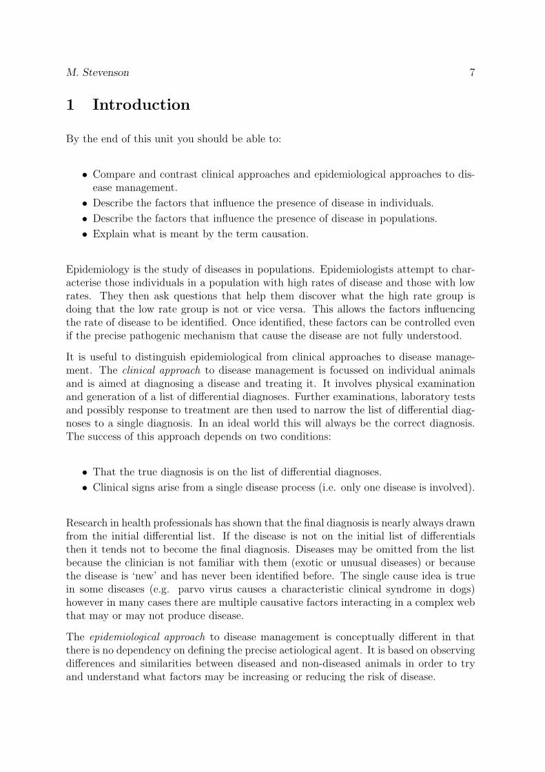
Individuals can be grouped or distinguished on a number of characteristics: age, sex,breed, coat colour and so on. An important component of epidemiological research isaimed at determining the influence of individual characteristics on the risk of disease.Figure 1 shows how mortality rate for drowning varied among children and young adultsin the USA during 1999. The rate was highest in those aged 1 - 4 years: an age whenchildren are mobile and curious about everything around them, even though they do notunderstand the hazards of deep water or how to survive if they fall in. What conclusionsdo we draw from this? Mortality as a result of drowning is highest in children aged 1 -4 years: preventive measures should be targeted at this age group.

Figure 1: Mortality from drowning by age: USA, 1999. Reproduced from: Hoyert et al. (2001).

1.2.2 Place

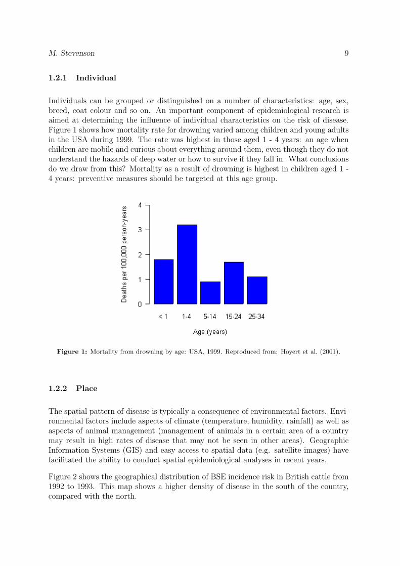
The spatial pattern of disease is typically a consequence of environmental factors. Envi-ronmental factors include aspects of climate (temperature, humidity, rainfall) as well asaspects of animal management (management of animals in a certain area of a countrymay result in high rates of disease that may not be seen in other areas). GeographicInformation Systems (GIS) and easy access to spatial data (e.g. satellite images) havefacilitated the ability to conduct spatial epidemiological analyses in recent years.

Figure 2 shows the geographical distribution of BSE incidence risk in British cattle from1992 to 1993. This map shows a higher density of disease in the south of the country,compared with the north.


��

��

��

��

��

��

Figure 2: Incidence risk of BSE across Great Britain (expressed as confirmed BSE cases per 100 adultcattle per square kilometre). Reproduced from Stevenson et al. (2000).

1.2.3 Time

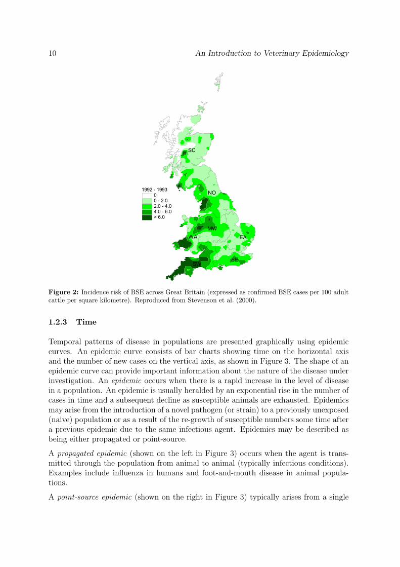
Temporal patterns of disease in populations are presented graphically using epidemiccurves. An epidemic curve consists of bar charts showing time on the horizontal axisand the number of new cases on the vertical axis, as shown in Figure 3. The shape of anepidemic curve can provide important information about the nature of the disease underinvestigation. An epidemic occurs when there is a rapid increase in the level of diseasein a population. An epidemic is usually heralded by an exponential rise in the number ofcases in time and a subsequent decline as susceptible animals are exhausted. Epidemicsmay arise from the introduction of a novel pathogen (or strain) to a previously unexposed(naive) population or as a result of the re-growth of susceptible numbers some time aftera previous epidemic due to the same infectious agent. Epidemics may be described asbeing either propagated or point-source.

A propagated epidemic (shown on the left in Figure 3) occurs when the agent is trans-mitted through the population from animal to animal (typically infectious conditions).Examples include influenza in humans and foot-and-mouth disease in animal popula-tions.

A point-source epidemic (shown on the right in Figure 3) typically arises from a single

M. Stevenson 11

source of exposure to a causal agent e.g. a batch of contaminated feed causing anoutbreak of salmonellosis in feedlot cattle, or a milk vacuum problem causing an outbreakof clinical mastitis in a herd of dairy cows. Epidemic curves for point-source epidemicsoften show a steep initial rise in case numbers and then a rapid falling off in the tail.

Figure 3: Epidemic curves. The plot on the left is typical of a propagated epidemic. The curve on theright is typical of a point source epidemic.

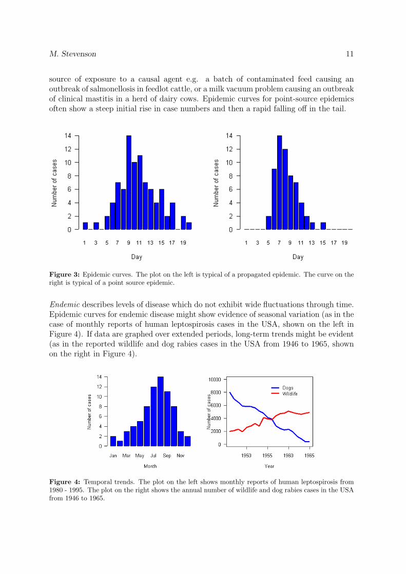
Endemic describes levels of disease which do not exhibit wide fluctuations through time.Epidemic curves for endemic disease might show evidence of seasonal variation (as in thecase of monthly reports of human leptospirosis cases in the USA, shown on the left inFigure 4). If data are graphed over extended periods, long-term trends might be evident(as in the reported wildlife and dog rabies cases in the USA from 1946 to 1965, shownon the right in Figure 4).

Figure 4: Temporal trends. The plot on the left shows monthly reports of human leptospirosis from1980 - 1995. The plot on the right shows the annual number of wildlife and dog rabies cases in the USAfrom 1946 to 1965.


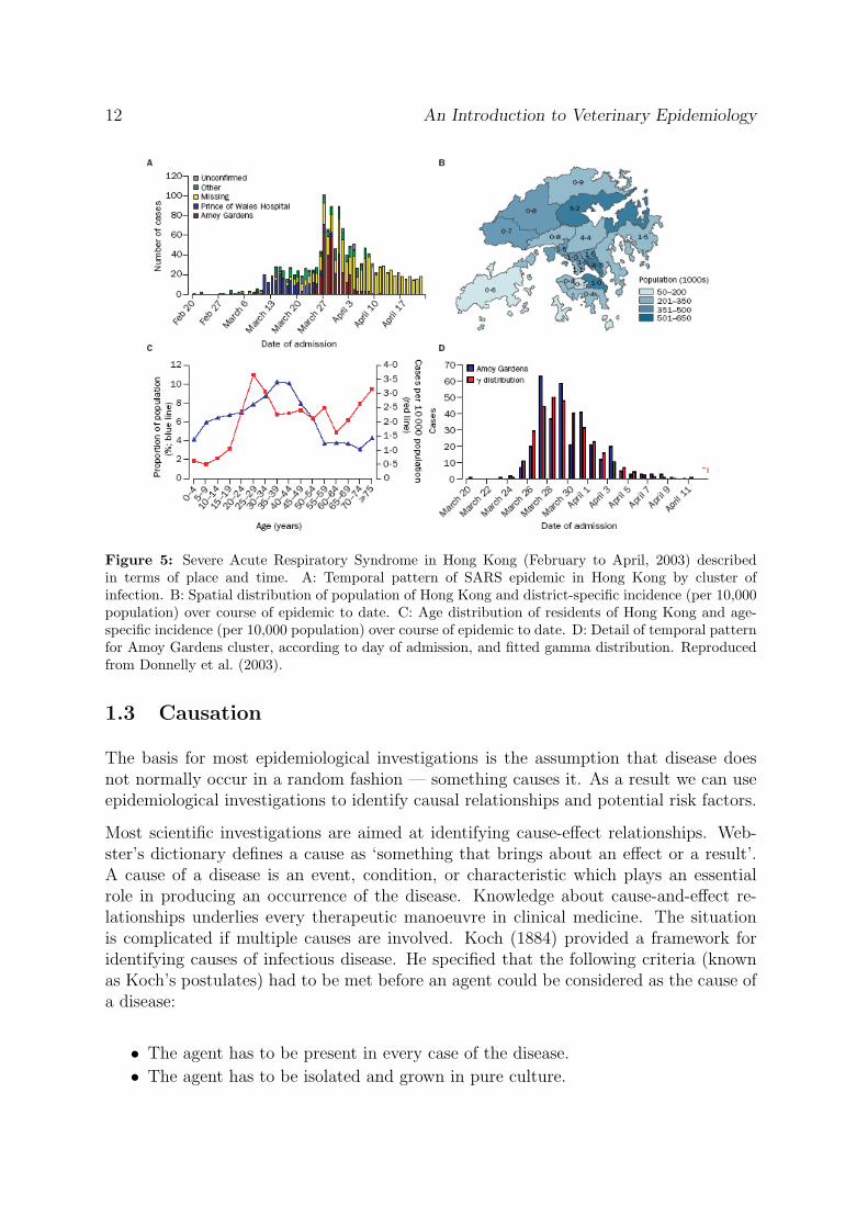
Figure 5: Severe Acute Respiratory Syndrome in Hong Kong (February to April, 2003) describedin terms of place and time. A: Temporal pattern of SARS epidemic in Hong Kong by cluster ofinfection. B: Spatial distribution of population of Hong Kong and district-specific incidence (per 10,000population) over course of epidemic to date. C: Age distribution of residents of Hong Kong and age-specific incidence (per 10,000 population) over course of epidemic to date. D: Detail of temporal patternfor Amoy Gardens cluster, according to day of admission, and fitted gamma distribution. Reproducedfrom Donnelly et al. (2003).

1.3 Causation

The basis for most epidemiological investigations is the assumption that disease doesnot normally occur in a random fashion — something causes it. As a result we can useepidemiological investigations to identify causal relationships and potential risk factors.

Most scientific investigations are aimed at identifying cause-effect relationships. Web-ster’s dictionary defines a cause as ‘something that brings about an effect or a result’.A cause of a disease is an event, condition, or characteristic which plays an essentialrole in producing an occurrence of the disease. Knowledge about cause-and-effect re-lationships underlies every therapeutic manoeuvre in clinical medicine. The situationis complicated if multiple causes are involved. Koch (1884) provided a framework foridentifying causes of infectious disease. He specified that the following criteria (knownas Koch’s postulates) had to be met before an agent could be considered as the cause ofa disease:

• The agent has to be present in every case of the disease.

• The agent has to be isolated and grown in pure culture.

M. Stevenson 13

• The agent has to cause disease when inoculated into a susceptible animal and theagent must then be able to be recovered from that animal and identified.

In the late nineteenth century Koch’s postulates brought a degree of order and disci-pline to the study of infectious diseases, although the key assumption of ‘one-agent-one-disease’ was highly restrictive (since it failed to take account of diseases with multipleaetiologic factors, multiple effects of single causes, carrier states, and non-agent factorssuch as age and breed).

Based on John Stuart Mill’s rules of inductive reasoning from 1856, Evan developed aunified concept of causation which is now the generally accepted means for identifyingcause-effect relationships in modern epidemiology. Evan’s unified concept of causationincludes the following criteria:

• The proportion of individuals with disease should be higher in those exposed tothe putative cause than in those not exposed.

• Exposure to the putative cause should be more common in cases than in thosewithout the disease.

• The number of new cases should be higher in those exposed to the putative causethan in those not exposed, as shown in prospective studies.

• Temporally, the disease should follow exposure to the putative cause.

• There should be a measurable biologic spectrum of host responses.

• The disease should be reproducible experimentally.

• Preventing or modifying the host response should decrease or eliminate the ex-pression of disease.

• Elimination of the putative cause should result in lower incidence of disease.

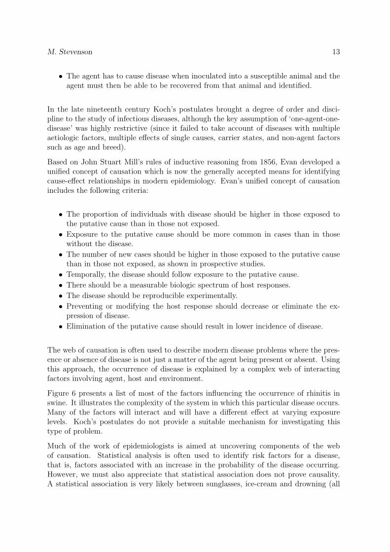
The web of causation is often used to describe modern disease problems where the pres-ence or absence of disease is not just a matter of the agent being present or absent. Usingthis approach, the occurrence of disease is explained by a complex web of interactingfactors involving agent, host and environment.

Figure 6 presents a list of most of the factors influencing the occurrence of rhinitis inswine. It illustrates the complexity of the system in which this particular disease occurs.Many of the factors will interact and will have a different effect at varying exposurelevels. Koch’s postulates do not provide a suitable mechanism for investigating thistype of problem.

Much of the work of epidemiologists is aimed at uncovering components of the webof causation. Statistical analysis is often used to identify risk factors for a disease,that is, factors associated with an increase in the probability of the disease occurring.However, we must also appreciate that statistical association does not prove causality.A statistical association is very likely between sunglasses, ice-cream and drowning (all


Figure 6: Web of causation for rhinitis in pigs.

are a function of outside temperature) but you would not claim that eating ice-creamor wearing sunglasses causes death by drowning.

If a statistical association is found between a factor and a disease it is then important todetermine if that factor may be causal. This is done by considering each of the criteriaof Evan’s unified concept of causation. This is where the endless process of scientificinference plays such a critical role. Develop a hypothesis and test it: if it is found to beincorrect, modify the hypothesis and test it again.

1.4 Historical examples in the development of epidemiology

1.4.1 Ignas Semmelweis

Ignas Semmelweis was director of the Viennese Maternity Hospital in the 1840s. Twoclinics made up the Viennese Maternity Hospital: one run by midwives and the secondrun by doctors and medical students. Perinatal mortality due to pueperal fever (septicmetritis) was 3 – 5 times higher in the doctor-run clinic compared with the midwife-run clinic with this relationship remaining constant over a 6 year period. In the 1840sprevailing medical opinion was that disease was essentially an act of God. In an attemptto uncover the reasons for the high mortality rate in the doctor-run clinic Semmelweisperformed a series of observational studies and arrived at the following conclusions:

• Mothers were becoming ill within 24 – 36 hours of delivery.

• Illness seemed to be associated with mothers that received a manual examination.

M. Stevenson 15

• Doctors and medical students were in the habit of performing necropsies (un-gloved) in the morning and then coming straight over to the maternity clinic inthe afternoon and performing vaginal examinations with unwashed hands.

• Midwives did not perform necropsies.

Semmelweis instituted a program of washing hands with chlorinated water upon entryto the maternity ward. This was implemented after much argument and opposition andat a time when hygiene was considered to be unrelated to disease. Death rates in thedoctor-run clinic decreased immediately.

1.4.2 John Snow

A major outbreak of cholera occurred in a small area of central London (Golden Square)in the 1840s with 500 fatal attacks occurring within a 10-day period. Snow spent muchof his life investigating cholera and collected a massive amount of data from this out-break. He found that most of the affected group had collected their drinking waterfrom a single water pump (the Broad Street pump). Snow applied pressure on the localcouncil to remove the handle from the Broad Street pump, hypothesising correctly thatcontaminated water from this pump was the source of infection.

Snow subsequently provided further evidence of the association between contaminateddrinking water and cholera with an eloquent study investigating the relationship betweencompanies supplying household water and cholera rates. During the 1840s London hadnumerous water companies that competed to supply household water. Customers chosewater companies largely at random. One company drew water only from a site on theThames River above all London sewerage outlets. The others drew water all alongthe river. Snow showed that those households that used the upriver water companyhad lower rates of cholera compared with those that used the other companies. Thissupported Snow’s hypothesis of water borne contamination causing the disease.

It was not until more than 30 years later that the causative organism of cholera (Vibriocholerae) was isolated.


2 Measures of health


• Differentiate between ratios, proportions and rates.

• Describe the terms incidence and prevalence, and use them appropriately.

• Describe the difference between risk and rate as applied to measures of incidence.

One of the most fundamental tasks in epidemiological research is to quantify the oc-currence of disease. This can be done by counting the number of affected individualshowever, to compare levels of disease among groups of individuals, time frames and lo-cations, we need to consider counts of cases in context of the size of the population fromwhich those cases arose.

A ratio defines the relative size of two quantities expressed by dividing one (numerator)by the other (denominator). Proportions, odds, and rates are ratios.

A proportion is a fraction in which the numerator is included in the denominator. Saywe have a herd of 100 cattle and 58 are found to be diseased. The proportion of diseasedanimals in this herd is 58 100 = 0.58 = 58

Odds are fractions where the numerator is not included in the denominator. Say wehave a herd of 100 cattle and 58 are found to be diseased. The odds of disease in thisherd is 58:42 or 1.4 to 1.

A rate is derived from three pieces of information: (1) a numerator: the number ofindividuals diseased or dead, (2) a denominator: the total number of animals (or animaltime) in the study group and/or period; and (3) a specified time period. To continuethe above example, we might say that the rate of disease in our herd over a 12-monthperiod was 58 cases per 100 cattle or 58 cases per 100 cattle-years at risk.

The term morbidity is used to refer to the extent of disease or disease frequency within adefined population. Two important measures of morbidity are prevalence and incidence.As epidemiologists we must take care to use these terms correctly.

2.1 Prevalence

The count of prevalent (existing) cases of a disease is the number of individuals in apopulation who are in the diseased state at a specified period of time. Prevalence is aproportion obtained by dividing the count of existing (prevalent) cases by the populationsize:

Prevalence =Number of existing cases

Size of population(2.1)

M. Stevenson 17

Prevalence can be interpreted as the probability of an individual from a populationhaving a disease at a given point in time.

In 1944 the cities of Newburgh and Kingston, New York agreed to participate in a study of the effectsof water fluoridation for prevention of tooth decay in children (Ast and Schlesinger, 1956). In 1944 thewater in both cities had low fluoride concentrations. In 1945, Newburgh began adding fluoride to itswater - increasing the concentration ten-fold while Kingston left its supply unchanged. To assess theeffect of water fluoridation on dental health, a survey was conducted among school children in bothcities during the 1954 - 1955 school year. One measure of dental decay in children 6 - 9 years of age waswhether at least one of a child’s 12 deciduous cuspids or first or second deciduous molars was missingor had clinical or X-ray evidence of tooth decay.

Of the 216 first-grade children examined in Kingston, 192 had evidence of tooth decay. Of the 184first-grade children examined in Newburgh 116 had evidence of tooth decay. Assuming complete surveycoverage, there were 192 prevalent cases of tooth decay among first-grade children in Kingston at thetime of the study. The prevalence of tooth decay was 192 ÷ 216 = 89% in Kingston and 116 ÷ 184 =63% in Newburgh.

2.2 Incidence

Incidence measures how frequently initially susceptible individuals become disease casesas they are observed over time. An incident case occurs when an individual changesfrom being susceptible to being diseased. The count of incident cases is the number ofsuch events that occur in a defined population during a specified time period. There aretwo ways to express incidence: incidence risk (also known as cumulative incidence) andincidence rate (also known as incidence density).

2.2.1 Incidence risk

Incidence risk (cumulative incidence) is the proportion of initially susceptible individualsin a population who become new cases during a defined time period.

Incidence risk =Number of new cases

Number of individuals initially at risk(2.2)

The defined time period may be arbitrarily fixed (e.g. 5-year incidence risk of arthritis)or it may vary among individuals (e.g. the lifetime incidence risk of arthritis). In aninvestigation of a localised epidemic the defined time period may be simply defined asthe duration of the epidemic.

• Individuals have to be disease-free at the beginning of the observation period tobe included in the numerator or denominator of this calculation.


• The time period to which the risk applies must be specified.

• The quantity is dimensionless and ranges from 0 to 1.

Individuals have to be disease-free at the beginning of the observation period to beincluded in the numerator or denominator of this calculation. Incidence risk may beinterpreted as an individual’s risk of contracting disease within the risk period. Thequantity is dimensionless, ranges from 0 to 1 and always requires a period referent (timeinterval).

Last year a herd of 121 cattle were tested for tuberculosis using the tuberculin test and all testednegative. This year the same 121 cattle were tested and 25 tested positive.

The incidence risk would then be 21 cases per 100 cattle for the 12-month period. We can also saythat the risk of an animal becoming positive to the tuberculin test for the 12-month period was21%. This is an expression of average risk applied to an individual (but estimated from the population).

The population at risk can either be closed or open. A closed population has no additionsduring the course of the study and no or few losses to follow-up. An open populationis where individuals are recruited (e.g. as births or purchases) and leave (e.g. as sales,deaths) throughout the course of the study period. Incidence risk is an appropriatemeasure of incidence when the population is closed and all subjects are followed for theentire study period.

If we don’t account for changes in the population size when dealing with open populationswe will tend to underestimate the incidence risk of disease: the size of our estimate ofthe population at risk will be larger than what it actually is. The actuarial (or life table)method of calculating incidence risk can be used to correct for losses to follow up in thissituation. Here, half of the number of animals lost to follow-up are subtracted from thedenominator. This results in a better-estimate of the size of population at risk, assumingthat the average withdrawal time occurs at the midpoint of the follow-up period.

If we are dealing with open populations, incidence risk cannot be measured directly, butcan be estimated (see below).

2.2.2 Incidence rate

Incidence rate (incidence density) is the number of new cases of disease that occurper unit of individual time at risk, during a defined time period. The denominator ofincidence rate is measured in units of animal (or person) time.

Incidence rate =Number of incident cases

Amount of at-risk experience(2.3)

M. Stevenson 19

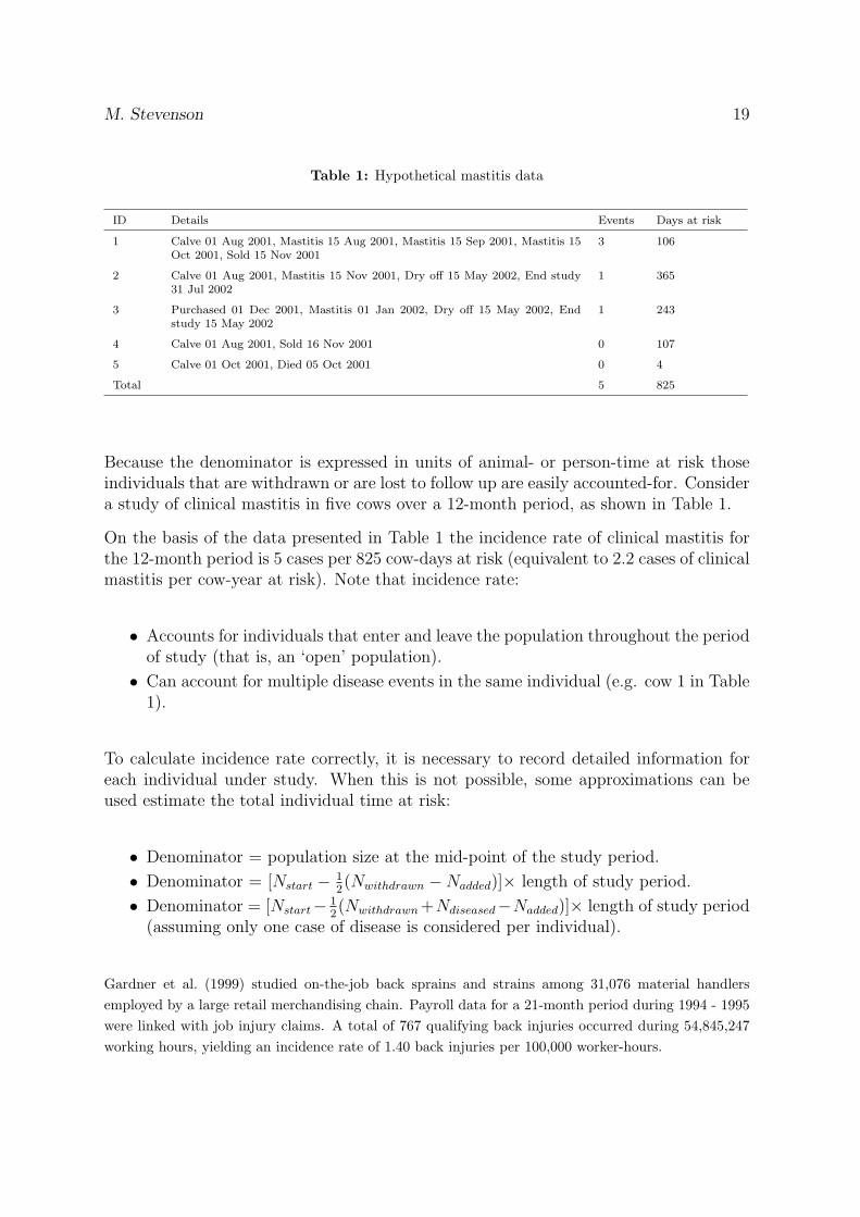
Table 1: Hypothetical mastitis data

ID Details Events Days at risk

1 Calve 01 Aug 2001, Mastitis 15 Aug 2001, Mastitis 15 Sep 2001, Mastitis 15Oct 2001, Sold 15 Nov 2001

3 106

2 Calve 01 Aug 2001, Mastitis 15 Nov 2001, Dry off 15 May 2002, End study31 Jul 2002

1 365

3 Purchased 01 Dec 2001, Mastitis 01 Jan 2002, Dry off 15 May 2002, Endstudy 15 May 2002

1 243

4 Calve 01 Aug 2001, Sold 16 Nov 2001 0 107

5 Calve 01 Oct 2001, Died 05 Oct 2001 0 4

Total 5 825

Because the denominator is expressed in units of animal- or person-time at risk thoseindividuals that are withdrawn or are lost to follow up are easily accounted-for. Considera study of clinical mastitis in five cows over a 12-month period, as shown in Table 1.

On the basis of the data presented in Table 1 the incidence rate of clinical mastitis forthe 12-month period is 5 cases per 825 cow-days at risk (equivalent to 2.2 cases of clinicalmastitis per cow-year at risk). Note that incidence rate:

• Accounts for individuals that enter and leave the population throughout the periodof study (that is, an ‘open’ population).

• Can account for multiple disease events in the same individual (e.g. cow 1 in Table1).

To calculate incidence rate correctly, it is necessary to record detailed information foreach individual under study. When this is not possible, some approximations can beused estimate the total individual time at risk:

• Denominator = population size at the mid-point of the study period.

• Denominator = [Nstart − 12(Nwithdrawn −Nadded)]× length of study period.

• Denominator = [Nstart− 12(Nwithdrawn +Ndiseased−Nadded)]× length of study period

(assuming only one case of disease is considered per individual).

Gardner et al. (1999) studied on-the-job back sprains and strains among 31,076 material handlersemployed by a large retail merchandising chain. Payroll data for a 21-month period during 1994 - 1995were linked with job injury claims. A total of 767 qualifying back injuries occurred during 54,845,247working hours, yielding an incidence rate of 1.40 back injuries per 100,000 worker-hours.


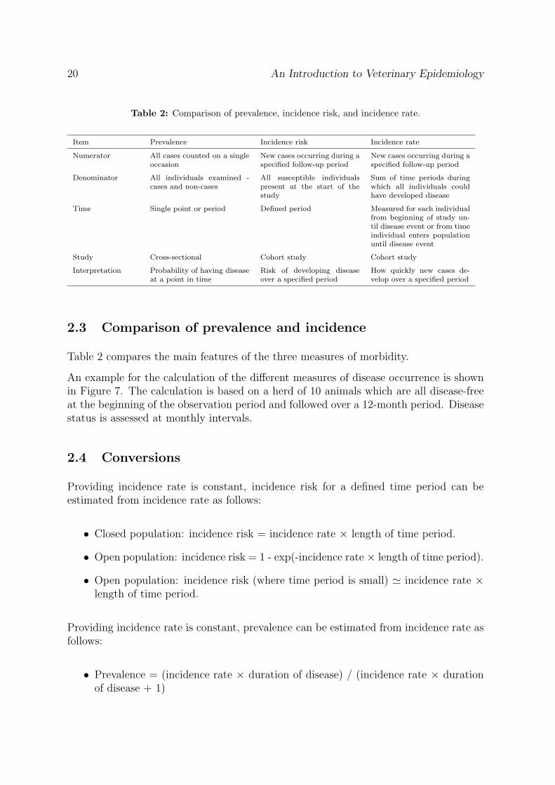
Table 2: Comparison of prevalence, incidence risk, and incidence rate.

Item Prevalence Incidence risk Incidence rate

Numerator All cases counted on a singleoccasion

New cases occurring during aspecified follow-up period

New cases occurring during aspecified follow-up period

Denominator All individuals examined -cases and non-cases

All susceptible individualspresent at the start of thestudy

Sum of time periods duringwhich all individuals couldhave developed disease

Time Single point or period Defined period Measured for each individualfrom beginning of study un-til disease event or from timeindividual enters populationuntil disease event

Study Cross-sectional Cohort study Cohort study

Interpretation Probability of having diseaseat a point in time

Risk of developing diseaseover a specified period

How quickly new cases de-velop over a specified period

2.3 Comparison of prevalence and incidence

Table 2 compares the main features of the three measures of morbidity.

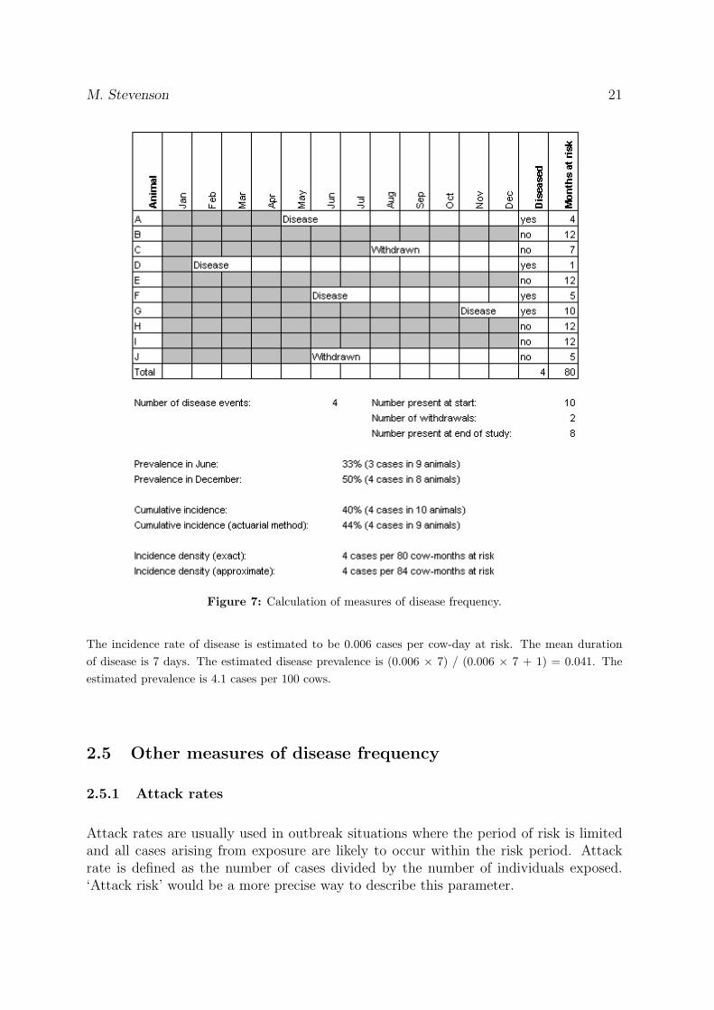
An example for the calculation of the different measures of disease occurrence is shownin Figure 7. The calculation is based on a herd of 10 animals which are all disease-freeat the beginning of the observation period and followed over a 12-month period. Diseasestatus is assessed at monthly intervals.

2.4 Conversions

Providing incidence rate is constant, incidence risk for a defined time period can beestimated from incidence rate as follows:

• Closed population: incidence risk = incidence rate × length of time period.

• Open population: incidence risk = 1 - exp(-incidence rate × length of time period).

• Open population: incidence risk (where time period is small) ' incidence rate ×length of time period.

Providing incidence rate is constant, prevalence can be estimated from incidence rate asfollows:

• Prevalence = (incidence rate × duration of disease) / (incidence rate × durationof disease + 1)

M. Stevenson 21

Figure 7: Calculation of measures of disease frequency.

The incidence rate of disease is estimated to be 0.006 cases per cow-day at risk. The mean durationof disease is 7 days. The estimated disease prevalence is (0.006 × 7) / (0.006 × 7 + 1) = 0.041. Theestimated prevalence is 4.1 cases per 100 cows.

2.5 Other measures of disease frequency

2.5.1 Attack rates

Attack rates are usually used in outbreak situations where the period of risk is limitedand all cases arising from exposure are likely to occur within the risk period. Attackrate is defined as the number of cases divided by the number of individuals exposed.‘Attack risk’ would be a more precise way to describe this parameter.


2.5.2 Secondary attack rates

Secondary attack rates are used to describe ‘infectiousness’. The assumption is thatthere is spread of an agent within an aggregation of individuals (e.g. a herd or a family)and that not all cases are a result of a common-source exposure. Secondary attackrates are the number of cases at the end of the study period less the number of initial(primary) cases divided by the size of the population that were initially at risk.

2.5.3 Mortality

Mortality risk (or rate) is an example of incidence where death is the outcome of interest.Cause-specific mortality risk is the incidence risk of fatal cases of a particular diseasein the population at risk of death from that disease. The denominator includes bothprevalent cases of the disease (that is, the individuals that haven’t died yet) as well asindividuals who are at risk of developing the disease.

2.5.4 Case fatality rate

Case fatality risk (or rate) refers to the incidence of death among individuals who de-velop the disease. Case fatality risk reflects the prognosis of disease among cases, whilemortality reflects the burden of deaths from the disease in the population as a whole.

2.5.5 Proportional mortality

As its name implies, proportional mortality is simply the proportion of all deaths thatare due to a particular cause for a specified population and time period:

Proportional mortality =Number of deaths from disease

Number of deaths from all causes(2.4)

2.6 Adjusted rates

Crude rates (incidence, mortality etc) provide a summary estimate of the level ofdisease in a study group as a whole — they take no account of the structure of thepopulation being studied.

If we have two colonies of mice and observe them for one day we might find the mortality rate in thefirst colony is 10 per 1,000 and the mortality rate in the second colony is 20 per 1,000. We mightinitially think that this difference is due to a difference in management, but it might also transpire thatthe first colony is comprised of mainly young mice and the second colony is comprised of mainly oldermice. The two colonies might be exactly the same in terms of standards of care and housing qualityand the difference in mortality solely due to a difference in age composition of the two populations.

M. Stevenson 23

Crude measures can only be used to compare two populations if the populations are similar withrespect to the characteristics that might affect disease occurrence.

Adjusted rates are used when comparing rates of health events affected by confoundingfactors. They are used when comparing different populations or for comparing trends ina given population over time. In human medicine, because the occurrence of many healthconditions is related to age, the most common adjustment for public health data is ageadjustment. In veterinary medicine age, breed, and production type (e.g. beef-dairy)are commonly used adjustment variables.

The age adjustment process removes differences in the age composition of two or morepopulations to allow comparisons between these populations to be made, independent oftheir age structure. For example, a countys age-adjusted death rate is the weighted aver-age of the age-specific death rates observed in that county, with the weights derived fromthe age distribution in an external population standard. Different standard populationshave different age distributions and the choice will affect the resulting age-adjusted rate.If the age-adjusted rates for different counties are calculated with the same weights (thatis, using the same population standard), the effect of any differences in the county’s agedistributions is removed.

There are two methods for adjusting disease rates: direct adjustment and indirect ad-justment.

2.6.1 Stratum-specific rates

• Calculation of stratum-specific rates is recommended before developing adjustedrates. This will identify whether or not the populations being compared showstratum-specific rates that are consistent. If the pattern is not consistent, use ofstratum-specific rates, rather than adjusted rates, are recommended.

• Stratum-specific rates are recommended for comparing defined subgroups betweenor within populations when rates are strongly stratum-dependent.

• Stratum-specific rates are recommended when specific causal or protective factorsor the prevalence of risk exposures are different for different levels of strata.

2.6.2 Comparing rates

Only compare rates when the numerator and denominator (i.e., events and population)are defined consistently over time and place. Look for:

• Consistency in definition of event.

• Consistency of surveillance intensity over time.

• Consistency of surveillance intensity among areas.


• If comparing stratum-adjusted rates, compare rates that have been adjusted tothe same standard population.

• When comparing age-specific rates, if the age categories are relatively large, it isimportant to consider the possibility of residual confounding by age.

2.6.3 Unstable rates due to small numbers

Rates based on small numbers of events can fluctuate widely from year to year forreasons other than a true change in the underlying frequency of occurrence of the event.Calculation of rates is not recommended when there are fewer than five events in thenumerator, because the calculated rate is unstable and exhibits wide confidence intervals.Small counts should be included, where possible, even if the rates are not reported, sothat the counts can be combined into larger totals (for example, three or five yearaverages) which would be more stable.

2.6.4 Direct adjustment

With direct adjustment the observed stratum-specific rates are known and an estimatedpopulation distribution is used as the basis for adjustment. A standard populationstructure is typically used: if we were stratifying by sex we might say that in a standardpopulation 50% of the total population would be allocated to the male strata and 50%to the female strata. The choice of the standard population for direct adjustment is notcrucial; however, where possible it is desirable to select a standard that is demographi-cally sensible. The directly adjusted count for the ith strata is then:

Directly adjusted counti = STDPi ×OBSRi (2.5)

Where:

STD Pi: the size of the standard population in the ith strataOBS Ri: the observed rate in the ith strata

Consider a study of leptospirosis seroprevalence in dogs, the details of which are shownin Table 3.

Table 3: Seroprevalence of leptospirosis in urban dogs, stratified by city.

City Positive Sampled Seroprevalence

Edinburgh 61 260 23%

Glasgow 69 251 27%

Total 130 511 25%

M. Stevenson 25

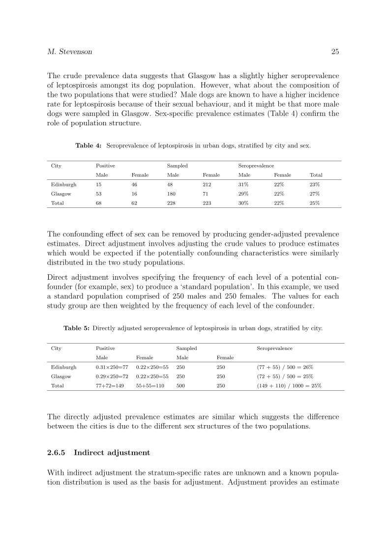
The crude prevalence data suggests that Glasgow has a slightly higher seroprevalenceof leptospirosis amongst its dog population. However, what about the composition ofthe two populations that were studied? Male dogs are known to have a higher incidencerate for leptospirosis because of their sexual behaviour, and it might be that more maledogs were sampled in Glasgow. Sex-specific prevalence estimates (Table 4) confirm therole of population structure.

Table 4: Seroprevalence of leptospirosis in urban dogs, stratified by city and sex.


Male Female Male Female Male Female Total

Edinburgh 15 46 48 212 31% 22% 23%

Glasgow 53 16 180 71 29% 22% 27%

Total 68 62 228 223 30% 22% 25%

The confounding effect of sex can be removed by producing gender-adjusted prevalenceestimates. Direct adjustment involves adjusting the crude values to produce estimateswhich would be expected if the potentially confounding characteristics were similarlydistributed in the two study populations.

Direct adjustment involves specifying the frequency of each level of a potential con-founder (for example, sex) to produce a ‘standard population’. In this example, we useda standard population comprised of 250 males and 250 females. The values for eachstudy group are then weighted by the frequency of each level of the confounder.

Table 5: Directly adjusted seroprevalence of leptospirosis in urban dogs, stratified by city.


Male Female Male Female

Edinburgh 0.31×250=77 0.22×250=55 250 250 (77 + 55) / 500 = 26%

Glasgow 0.29×250=72 0.22×250=55 250 250 (72 + 55) / 500 = 25%

Total 77+72=149 55+55=110 500 250 (149 + 110) / 1000 = 25%

The directly adjusted prevalence estimates are similar which suggests the differencebetween the cities is due to the different sex structures of the two populations.

2.6.5 Indirect adjustment

With indirect adjustment the stratum-specific rates are unknown and a known popula-tion distribution is used as the basis for adjustment. Adjustment provides an estimate


of the expected number of cases, given the stratum-specific population size. It is usualto divide the observed number of disease cases by the expected number to yield a stan-dardised morbidity/mortality ratio (SMR).

Indirectly adjusted counti = STDRi ×OBSPi (2.6)

Where:

STD Ri: the standard rate in the ith strata of the populationOBS Pi: the observed population size in the ith strata

We know that the prevalence of a given disease throughout a country is 0.01%. For each administrativeregion within the country, the expected number of disease cases is 0.01% × the size of the region-levelpopulation size. Thus, if we have a region with 20,000 animals the expected number of cases of diseasein this region will be 0.01% × 20,000 = 2. If the actual number of cases of disease in this region is 5,then this region’s Standardised Mortality (Morbidity) Ratio for the disease is 5 ÷ 2 = 2.5. That is,there were 2.5 times more cases of disease in this region, compared with the number of cases we wereexpecting.

M. Stevenson 27

��

(a) SMR: pre-control cohort

��

(b) SMR: post-control cohort

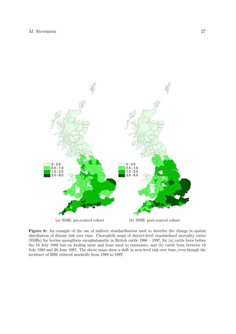
Figure 8: An example of the use of indirect standardisation used to describe the change in spatialdistribution of disease risk over time. Choropleth maps of district-level standardised mortality ratios(SMRs) for bovine spongiform encephalopathy in British cattle 1986 – 1997, for (a) cattle born beforethe 18 July 1988 ban on feeding meat and bone meal to ruminants, and (b) cattle born between 18July 1988 and 30 June 1997. The above maps show a shift in area-level risk over time, even though theincidence of BSE reduced markedly from 1988 to 1997.


3 Study design


• Describe the difference between descriptive and analytical epidemiological studies(giving examples of each).

• Describe the major features of randomised clinical trials, cohort studies, case-control studies, and cross-sectional studies.

• Describe the strengths and weaknesses of clinical trials, cohort studies, case-controlstudies, and cross-sectional studies.

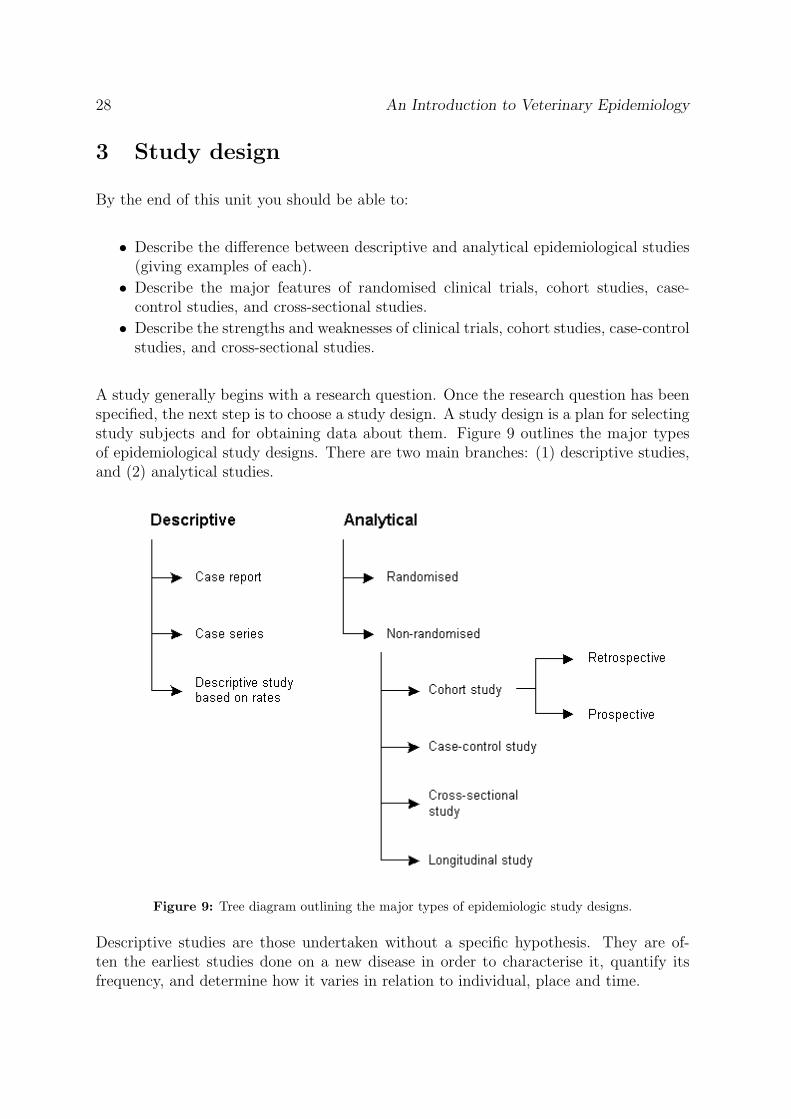
A study generally begins with a research question. Once the research question has beenspecified, the next step is to choose a study design. A study design is a plan for selectingstudy subjects and for obtaining data about them. Figure 9 outlines the major typesof epidemiological study designs. There are two main branches: (1) descriptive studies,and (2) analytical studies.

Figure 9: Tree diagram outlining the major types of epidemiologic study designs.

Descriptive studies are those undertaken without a specific hypothesis. They are of-ten the earliest studies done on a new disease in order to characterise it, quantify itsfrequency, and determine how it varies in relation to individual, place and time.

M. Stevenson 29

Analytical studies are undertaken to test specific hypotheses. There are two main typesof analytical studies: (1) randomised studies — where subjects are randomly allocated toexposure groups, and (2) non-randomised studies - where no formal chance mechanismgoverns which subjects are exposed and which are not.

3.1 Descriptive studies

The hallmark of a descriptive study is that it is undertaken without a specific hypothesis.

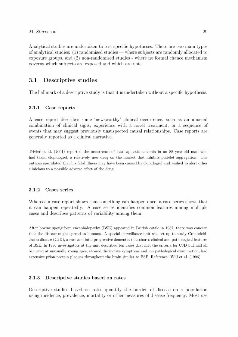
3.1.1 Case reports

A case report describes some ‘newsworthy’ clinical occurrence, such as an unusualcombination of clinical signs, experience with a novel treatment, or a sequence ofevents that may suggest previously unsuspected causal relationships. Case reports aregenerally reported as a clinical narrative.

Trivier et al. (2001) reported the occurrence of fatal aplastic anaemia in an 88 year-old man whohad taken clopidogrel, a relatively new drug on the market that inhibits platelet aggregation. Theauthors speculated that his fatal illness may have been caused by clopidogrel and wished to alert otherclinicians to a possible adverse effect of the drug.

3.1.2 Cases series

Whereas a case report shows that something can happen once, a case series shows thatit can happen repeatedly. A case series identifies common features among multiplecases and describes patterns of variability among them.

After bovine spongiform encephalopathy (BSE) appeared in British cattle in 1987, there was concernthat the disease might spread to humans. A special surveillance unit was set up to study Creutzfeld-Jacob disease (CJD), a rare and fatal progressive dementia that shares clinical and pathological featuresof BSE. In 1996 investigators at the unit described ten cases that met the criteria for CJD but had alloccurred at unusually young ages, showed distinctive symptoms and, on pathological examination, hadextensive prion protein plaques throughout the brain similar to BSE. Reference: Will et al. (1996)

3.1.3 Descriptive studies based on rates

Descriptive studies based on rates quantify the burden of disease on a populationusing incidence, prevalence, mortality or other measures of disease frequency. Most use


data from existing sources (such as birth and death certificates, disease registries orsurveillance systems). Descriptive studies can be a rich source of hypotheses that leadlater to analytic studies.

Schwarz et al. (1994) conducted a descriptive epidemiological study of injuries in a predominantlyAfrican-American part of Philadelphia. An injury surveillance system was set up in a hospitalemergency centre. Denominator information came from US census data. These authors found a highincidence of intentional interpersonal injury in this area of the city.

3.2 Analytical studies

Analytical studies are undertaken to test a hypothesis. In epidemiology the hypothesistypically concerns whether a certain exposure causes a certain outcome — e.g. doescigarette smoking cause lung cancer?

The term exposure is used to refer to any trait, behaviour, environment factor or othercharacteristic being measured as a possible cause of disease. Synonyms for exposure are:potential risk factor, putative cause, independent variable, and predictor. The termoutcome generally refers to the occurrence of disease. Synonyms for outcome are: effect,end-point, and dependent variable.

The hypothesis in an analytic study is whether an exposure actually causes an outcome(not merely whether the two are associated). Each of Evan’s unified concept of causationare usually required to be met to support a case for causality, but probably the mostimportant is that exposure must precede the outcome in time.

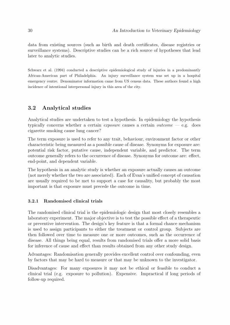
3.2.1 Randomised clinical trials

The randomised clinical trial is the epidemiologic design that most closely resembles alaboratory experiment. The major objective is to test the possible effect of a therapeuticor preventive intervention. The design’s key feature is that a formal chance mechanismis used to assign participants to either the treatment or control group. Subjects arethen followed over time to measure one or more outcomes, such as the occurrence ofdisease. All things being equal, results from randomised trials offer a more solid basisfor inference of cause and effect than results obtained from any other study design.

Advantages: Randomisation generally provides excellent control over confounding, evenby factors that may be hard to measure or that may be unknown to the investigator.

Disadvantages: For many exposures it may not be ethical or feasible to conduct aclinical trial (e.g. exposure to pollution). Expensive. Impractical if long periods offollow-up required.

M. Stevenson 31

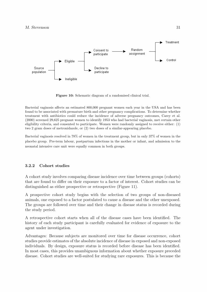
Figure 10: Schematic diagram of a randomised clinical trial.

Bacterial vaginosis affects an estimated 800,000 pregnant women each year in the USA and has beenfound to be associated with premature birth and other pregnancy complications. To determine whethertreatment with antibiotics could reduce the incidence of adverse pregnancy outcomes, Carey et al.(2000) screened 29,625 pregnant women to identify 1953 who had bacterial vaginosis, met certain othereligibility criteria, and consented to participate. Women were randomly assigned to receive either: (1)two 2 gram doses of metronidazole, or (2) two doses of a similar-appearing placebo.

Bacterial vaginosis resolved in 78% of women in the treatment group, but in only 37% of women in theplacebo group. Pre-term labour, postpartum infections in the mother or infant, and admission to theneonatal intensive care unit were equally common in both groups.

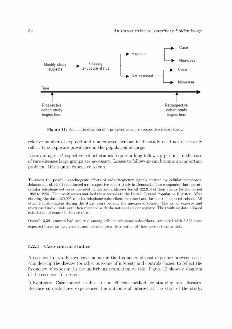
3.2.2 Cohort studies

A cohort study involves comparing disease incidence over time between groups (cohorts)that are found to differ on their exposure to a factor of interest. Cohort studies can bedistinguished as either prospective or retrospective (Figure 11).

A prospective cohort study begins with the selection of two groups of non-diseasedanimals, one exposed to a factor postulated to cause a disease and the other unexposed.The groups are followed over time and their change in disease status is recorded duringthe study period.

A retrospective cohort starts when all of the disease cases have been identified. Thehistory of each study participant is carefully evaluated for evidence of exposure to theagent under investigation.

Advantages: Because subjects are monitored over time for disease occurrence, cohortstudies provide estimates of the absolute incidence of disease in exposed and non-exposedindividuals. By design, exposure status is recorded before disease has been identified.In most cases, this provides unambiguous information about whether exposure precededdisease. Cohort studies are well-suited for studying rare exposures. This is because the


Figure 11: Schematic diagram of a prospective and retrospective cohort study.

relative number of exposed and non-exposed persons in the study need not necessarilyreflect true exposure prevalence in the population at large.

Disadvantages: Prospective cohort studies require a long follow-up period. In the caseof rare diseases large groups are necessary. Losses to follow-up can become an importantproblem. Often quite expensive to run.

To assess the possible carcinogenic effects of radio-frequency signals emitted by cellular telephones,Johansen et al. (2001) conducted a retrospective cohort study in Denmark. Two companies that operatecellular telephone networks provided names and addresses for all 522,914 of their clients for the period1982 to 1995. The investigators matched these records to the Danish Central Population Register. Aftercleaning the data 420,095 cellular telephone subscribers remained and formed the exposed cohort. Allother Danish citizens during the study years became the unexposed cohort. The list of exposed andunexposed individuals were then matched with the national cancer registry. The resulting data allowedcalculation of cancer incidence rates.

Overall, 3,391 cancers had occurred among cellular telephone subscribers, compared with 3,825 casesexpected based on age, gender, and calendar-year distribution of their person time at risk.

3.2.3 Case-control studies

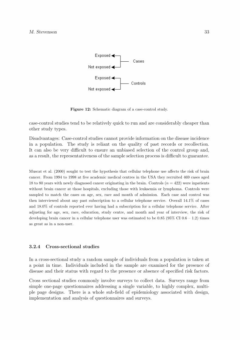
A case-control study involves comparing the frequency of past exposure between caseswho develop the disease (or other outcome of interest) and controls chosen to reflect thefrequency of exposure in the underlying population at risk. Figure 12 shows a diagramof the case-control design.

Advantages: Case-control studies are an efficient method for studying rare diseases.Because subjects have experienced the outcome of interest at the start of the study,

M. Stevenson 33

Figure 12: Schematic diagram of a case-control study.

case-control studies tend to be relatively quick to run and are considerably cheaper thanother study types.

Disadvantages: Case-control studies cannot provide information on the disease incidencein a population. The study is reliant on the quality of past records or recollection.It can also be very difficult to ensure an unbiased selection of the control group and,as a result, the representativeness of the sample selection process is difficult to guarantee.

Muscat et al. (2000) sought to test the hypothesis that cellular telephone use affects the risk of braincancer. From 1994 to 1998 at five academic medical centres in the USA they recruited 469 cases aged18 to 80 years with newly diagnosed cancer originating in the brain. Controls (n = 422) were inpatientswithout brain cancer at those hospitals, excluding those with leukaemia or lymphoma. Controls weresampled to match the cases on age, sex, race and month of admission. Each case and control wasthen interviewed about any past subscription to a cellular telephone service. Overall 14.1% of casesand 18.0% of controls reported ever having had a subscription for a cellular telephone service. Afteradjusting for age, sex, race, education, study centre, and month and year of interview, the risk ofdeveloping brain cancer in a cellular telephone user was estimated to be 0.85 (95% CI 0.6 – 1.2) timesas great as in a non-user.

3.2.4 Cross-sectional studies

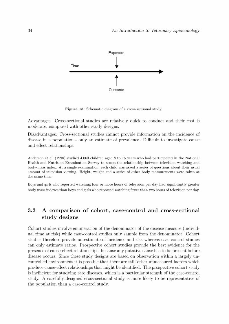
In a cross-sectional study a random sample of individuals from a population is taken ata point in time. Individuals included in the sample are examined for the presence ofdisease and their status with regard to the presence or absence of specified risk factors.

Cross sectional studies commonly involve surveys to collect data. Surveys range fromsimple one-page questionnaires addressing a single variable, to highly complex, multi-ple page designs. There is a whole sub-field of epidemiology associated with design,implementation and analysis of questionnaires and surveys.


Figure 13: Schematic diagram of a cross-sectional study.

Advantages: Cross-sectional studies are relatively quick to conduct and their cost ismoderate, compared with other study designs.

Disadvantages: Cross-sectional studies cannot provide information on the incidence ofdisease in a population - only an estimate of prevalence. Difficult to investigate causeand effect relationships.

Anderson et al. (1998) studied 4,063 children aged 8 to 16 years who had participated in the NationalHealth and Nutrition Examination Survey to assess the relationship between television watching andbody-mass index. At a single examination, each child was asked a series of questions about their usualamount of television viewing. Height, weight and a series of other body measurements were taken atthe same time.

Boys and girls who reported watching four or more hours of television per day had significantly greaterbody mass indexes than boys and girls who reported watching fewer than two hours of television per day.

3.3 A comparison of cohort, case-control and cross-sectionalstudy designs

Cohort studies involve enumeration of the denominator of the disease measure (individ-ual time at risk) while case-control studies only sample from the denominator. Cohortstudies therefore provide an estimate of incidence and risk whereas case-control studiescan only estimate ratios. Prospective cohort studies provide the best evidence for thepresence of cause-effect relationships, because any putative cause has to be present beforedisease occurs. Since these study designs are based on observation within a largely un-controlled environment it is possible that there are still other unmeasured factors whichproduce cause-effect relationships that might be identified. The prospective cohort studyis inefficient for studying rare diseases, which is a particular strength of the case-controlstudy. A carefully designed cross-sectional study is more likely to be representative ofthe population than a case-control study.

M. Stevenson 35

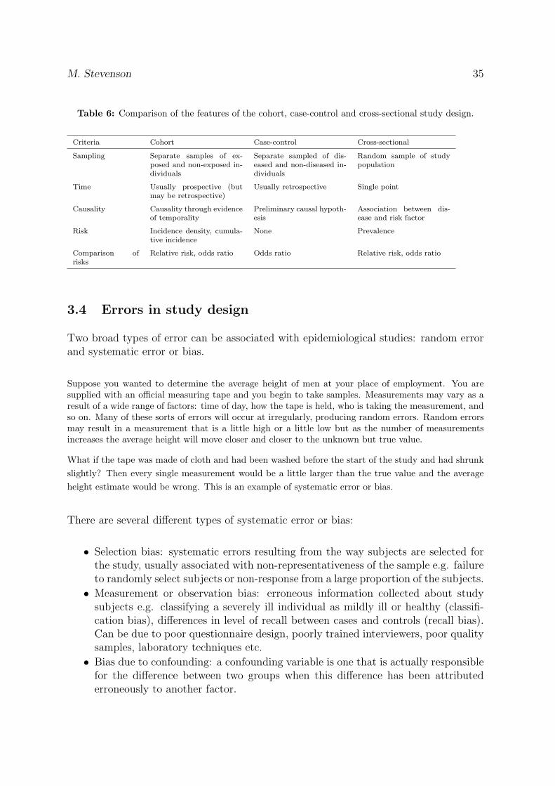
Table 6: Comparison of the features of the cohort, case-control and cross-sectional study design.

Criteria Cohort Case-control Cross-sectional

Sampling Separate samples of ex-posed and non-exposed in-dividuals

Separate sampled of dis-eased and non-diseased in-dividuals

Random sample of studypopulation

Time Usually prospective (butmay be retrospective)

Usually retrospective Single point

Causality Causality through evidenceof temporality

Preliminary causal hypoth-esis

Association between dis-ease and risk factor

Risk Incidence density, cumula-tive incidence

None Prevalence

Comparison ofrisks

Relative risk, odds ratio Odds ratio Relative risk, odds ratio

3.4 Errors in study design

Two broad types of error can be associated with epidemiological studies: random errorand systematic error or bias.

Suppose you wanted to determine the average height of men at your place of employment. You aresupplied with an official measuring tape and you begin to take samples. Measurements may vary as aresult of a wide range of factors: time of day, how the tape is held, who is taking the measurement, andso on. Many of these sorts of errors will occur at irregularly, producing random errors. Random errorsmay result in a measurement that is a little high or a little low but as the number of measurementsincreases the average height will move closer and closer to the unknown but true value.

What if the tape was made of cloth and had been washed before the start of the study and had shrunkslightly? Then every single measurement would be a little larger than the true value and the averageheight estimate would be wrong. This is an example of systematic error or bias.

There are several different types of systematic error or bias:

• Selection bias: systematic errors resulting from the way subjects are selected forthe study, usually associated with non-representativeness of the sample e.g. failureto randomly select subjects or non-response from a large proportion of the subjects.

• Measurement or observation bias: erroneous information collected about studysubjects e.g. classifying a severely ill individual as mildly ill or healthy (classifi-cation bias), differences in level of recall between cases and controls (recall bias).Can be due to poor questionnaire design, poorly trained interviewers, poor qualitysamples, laboratory techniques etc.

• Bias due to confounding: a confounding variable is one that is actually responsiblefor the difference between two groups when this difference has been attributederroneously to another factor.


During the analysis of data from a study of leptospirosis in dairy farm workers in New Zealand investi-gators found that wearing an apron during milking was associated with an increased risk of contractingleptospirosis. But before publicising this result, it was found that the risk of infection increased withherd size, and herd managers of larger herds were found to be more likely to wear aprons duringmilking than herd managers of smaller herds. The investigators concluded that the apparent associa-tion between wearing an apron and leptospirosis infection was due to the confounding effect of herd size.

Biases can be difficult to identify and deal with. Some biases are unavoidable and willneed to be dealt with during the analysis. Some can be prevented by careful study design,training of personnel involved in conducting the study and monitoring of procedures andequipment throughout the study.

M. Stevenson 37

4 Measures of association


• Given disease count data, construct a 2 × 2 table and explain how to calculate thefollowing measures of association: relative risk, odds ratio, attributable rate, andattributable fraction.

• Interpret the following measures of association: relative risk, odds ratio, at-tributable rate, and attributable fraction.

• Describe those situations where relative risk is not a valid measure of associationbetween exposure and outcome.

Risk is the probability that an event will happen. A characteristic or factor that influ-ences whether or not an event occurs, is called a risk factor.

• Worn tyres are a risk factor for motor vehicle accidents.

• High blood pressure is a risk factor for coronary heart disease.

• Vaccination is a protective risk factor in that it usually reduces the risk of disease.

If we identify those risk factors that are causally associated with an increased likelihoodof disease and those causally associated with a decreased likelihood of disease, then weare in a good position to make recommendations about health management. Much ofepidemiological research is concerned with estimating and quantifying risk factors fordisease.

Associations between putative risk factors (exposures) and an outcome (usually a dis-ease) can be investigated using analytical observational studies. Consider a study wheresubjects are disease free at the start of the study and all are monitored for disease oc-currence for a specified time period. If both exposure and outcome are binary variables(yes or no), the results can be presented in the format of a 2 × 2 table, as shown below:

Diseased Non-diseased Total

Exposed a b a + b

Non-exposed c d c + d

Total a + c b + d a+b+c+d = n

Based on data in this ‘standard’ 2 × 2 table format, various measures of association canbe calculated. These fall into three main categories: (1) measures strength, (2) measuresof effect, and (3) measures of total effect. To calculate these parameters, it helps to workout some summary parameters:

Incidence risk in the exposed population: RE = a/(a + b)Incidence risk in the non-exposed population: RO = c/(c + d)


Incidence risk in the total population: RTOTAL = (a + c)/(a + b + c + d) Odds of diseasein the exposed population: OE = a/bOdds of disease in the non-exposed population: OO = c/d

Observed associations are not always causal and/or may be estimated with bias. Theinterpretation of the measures of association described below assumes that relationshipsare causal and estimated without bias.

4.1 Measures of strength

4.1.1 Risk ratio

Where incidence risk has been measured, the risk ratio is defined as the ratio of therisk of disease (i.e. the incidence risk) in the exposed group to the risk of disease in theunexposed group. Using the notation defined above, risk ratio (RR) is calculated as:

RR =RE

RO

(4.1)

The risk ratio provides an estimate of how many times more likely exposed individualsare to experience disease, relative to non-exposed individuals. If the risk ratio equals 1,then the risks of disease in the exposed and non-exposed groups are equal. If the riskratio is greater than 1, then exposure increases the risk of disease with greater departuresfrom 1 indicative of a stronger effect. If the risk ratio is less than 1, exposure reducesthe risk of disease and exposure is said to be protective. Risk ratio cannot be estimatedin case-control studies, as these studies do not allow calculation of risks. Odds ratiosare used instead — see below.

Risk ratios range between 0 and ∞.

4.1.2 Incidence rate ratio

In a study where incidence rate has been measured (rather than incidence risk), theincidence rate ratio (also known as the rate ratio) can be calculated. This is the ratioof the incidence rate in the exposed group to that in the non-exposed group. Incidencerate ratio is interpreted in the same way as risk ratio.

The term relative risk (RR) is used as a synonym for both risk ratio and incidence rateratio.

M. Stevenson 39

4.1.3 Odds ratio

The odds ratio (OR) is an estimate of relative risk and is interpreted in the same wayas relative risk. If the incidence of disease in a case-control study is relatively low inboth exposed and non-exposed individuals, then a will be small relative to b and c willbe small relative to d. As a result:

OR =OE

OO

=ad

bc(4.2)

The odds ratio is the odds of disease, given exposure. When the number of cases ofdisease is low relative to the number of non-cases (i.e. the disease is rare), then the ORapproximates risk ratio. If the incidence of disease is relatively low in both exposed andnon-exposed individuals, then a will be small relative to b and c will be small relativeto d. As a result:

RR =a/(a + b)

c/(c + d)' a/b

c/d=

ad

bc= OR (4.3)

4.2 Measures of effect in the exposed population

4.2.1 Attributable rate (rate)

Also known as the risk difference, attributable risk (or rate) is defined as the increase(or decrease) in the risk or rate of disease in the exposed group that is attributableto exposure. Attributable risk (unlike risk ratio) describes the absolute quantity of theoutcome measure that is associated with the exposure. Using the notation defined above,attributable risk (AR) is calculated as:

AR = RE −RO (4.4)

4.2.2 Attributable fraction

Attributable fraction (also known as the attributable proportion in exposed subjects)is the proportion of disease in the exposed group that is due to exposure. Using thenotation defined above, attributable fraction (AF) is calculated as:

AF =(RE −RO)

RE

(4.5)

AF =(RR− 1)

RR(4.6)


For case-control studies, attributable fraction can be estimated:

AFest '(OR− 1)

OR(4.7)

This approximation is appropriate if: (1) disease incidence is low, or (2) odds ratios werederived from a case control study where incidence density sampling was used.

In vaccine trials, vaccine efficacy is defined as the proportion of disease prevented by the vaccine invaccinated individuals (equivalent to the proportion of disease in unvaccinated individuals due to notbeing vaccinated), which is the attributable fraction. A case-control study investigating the effect oforal vaccination on the presence or absence of rabies in foxes was conducted. The following results wereobtained:

Rabies + Rabies - Total

Vaccination - 18 30 48

Vaccination + 12 46 58

Total 30 76 106

The odds of rabies in the unvaccinated group was 2.3 times the odds of rabies in the vaccinated group(OR = 2.30). Fifty six percent of rabies cases in unvaccinated foxes was due to not being vaccinated(AFest = 0.56).

4.3 Measures of effect in the total population

4.3.1 Population attributable risk (rate)

Population attributable rate is the increase (or decrease) in risk or rate of disease inthe population that is attributable to exposure. Using the notation defined above,population attributable rate (PAR) is calculated as:

PAR = RTOTAL −RO (4.8)

4.3.2 Population attributable fraction

Population attributable fraction (also known as the aetiologic fraction) is the proportionof disease in the population that is due to the exposure. Using the notation definedabove, the population attributable fraction (PAF) is calculated as:

PAR =(RTOTAL −RO)

RTOTAL

(4.9)

M. Stevenson 41

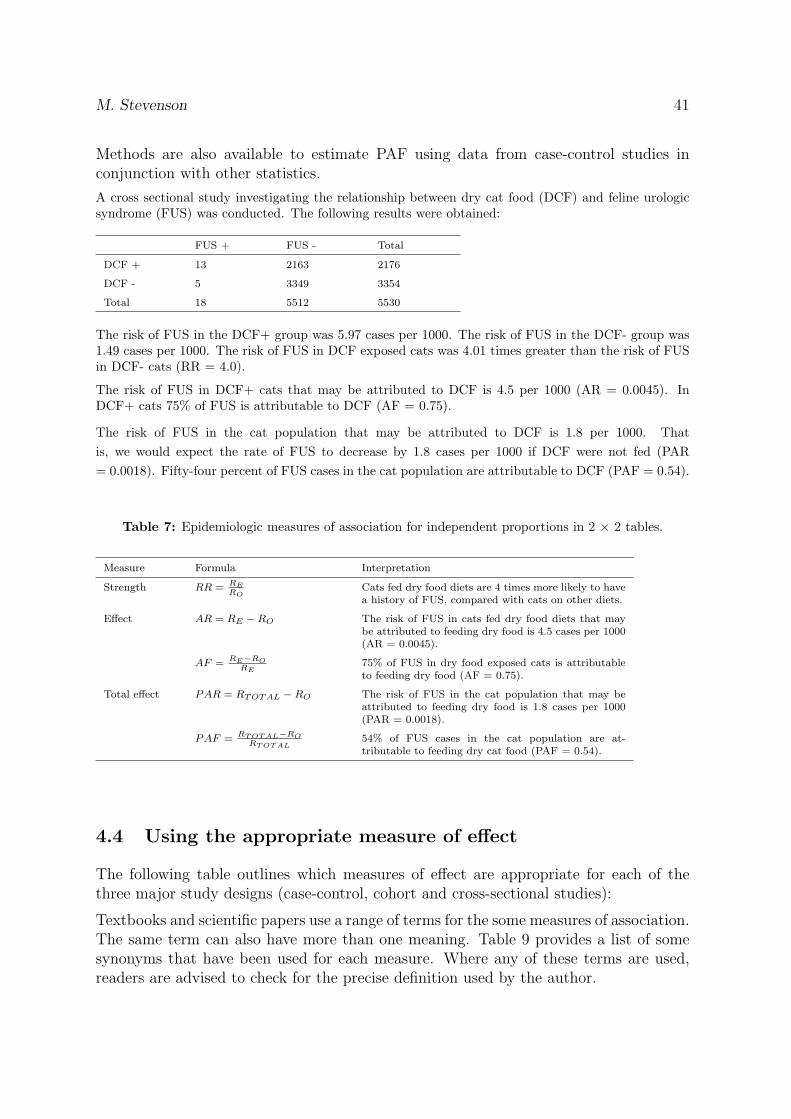
Methods are also available to estimate PAF using data from case-control studies inconjunction with other statistics.

A cross sectional study investigating the relationship between dry cat food (DCF) and feline urologicsyndrome (FUS) was conducted. The following results were obtained:

FUS + FUS - Total

DCF + 13 2163 2176

DCF - 5 3349 3354

Total 18 5512 5530

The risk of FUS in the DCF+ group was 5.97 cases per 1000. The risk of FUS in the DCF- group was1.49 cases per 1000. The risk of FUS in DCF exposed cats was 4.01 times greater than the risk of FUSin DCF- cats (RR = 4.0).

The risk of FUS in DCF+ cats that may be attributed to DCF is 4.5 per 1000 (AR = 0.0045). InDCF+ cats 75% of FUS is attributable to DCF (AF = 0.75).

The risk of FUS in the cat population that may be attributed to DCF is 1.8 per 1000. Thatis, we would expect the rate of FUS to decrease by 1.8 cases per 1000 if DCF were not fed (PAR= 0.0018). Fifty-four percent of FUS cases in the cat population are attributable to DCF (PAF = 0.54).

Table 7: Epidemiologic measures of association for independent proportions in 2 × 2 tables.

Measure Formula Interpretation

Strength RR = RERO

Cats fed dry food diets are 4 times more likely to havea history of FUS, compared with cats on other diets.

Effect AR = RE −RO The risk of FUS in cats fed dry food diets that maybe attributed to feeding dry food is 4.5 cases per 1000(AR = 0.0045).

AF = RE−RORE

75% of FUS in dry food exposed cats is attributableto feeding dry food (AF = 0.75).

Total effect PAR = RTOTAL −RO The risk of FUS in the cat population that may beattributed to feeding dry food is 1.8 cases per 1000(PAR = 0.0018).

PAF = RT OT AL−RORT OT AL

54% of FUS cases in the cat population are at-tributable to feeding dry cat food (PAF = 0.54).

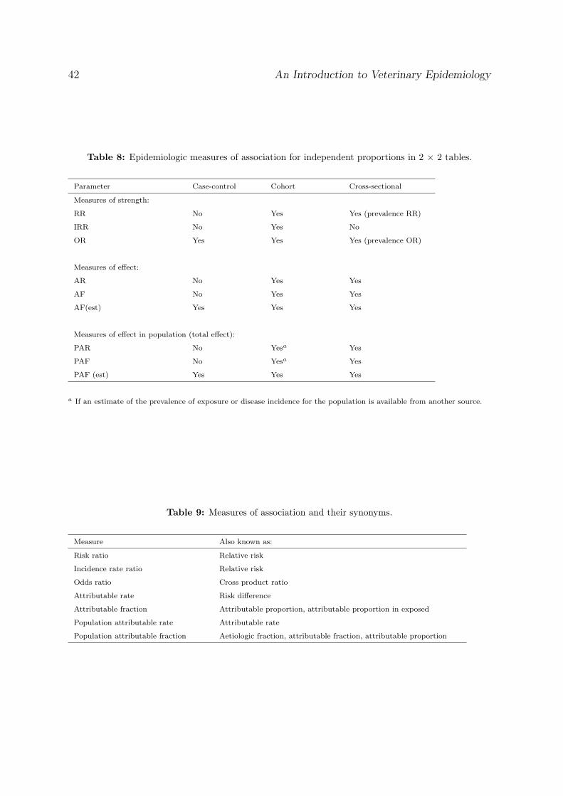
4.4 Using the appropriate measure of effect

The following table outlines which measures of effect are appropriate for each of thethree major study designs (case-control, cohort and cross-sectional studies):

Textbooks and scientific papers use a range of terms for the some measures of association.The same term can also have more than one meaning. Table 9 provides a list of somesynonyms that have been used for each measure. Where any of these terms are used,readers are advised to check for the precise definition used by the author.


Table 8: Epidemiologic measures of association for independent proportions in 2 × 2 tables.

Parameter Case-control Cohort Cross-sectional

Measures of strength:

RR No Yes Yes (prevalence RR)

IRR No Yes No

OR Yes Yes Yes (prevalence OR)

Measures of effect:

AR No Yes Yes

AF No Yes Yes

AF(est) Yes Yes Yes

Measures of effect in population (total effect):

PAR No Yesa Yes

PAF No Yesa Yes

PAF (est) Yes Yes Yes

a If an estimate of the prevalence of exposure or disease incidence for the population is available from another source.

Table 9: Measures of association and their synonyms.

Measure Also known as:

Risk ratio Relative risk

Incidence rate ratio Relative risk

Odds ratio Cross product ratio

Attributable rate Risk difference

Attributable fraction Attributable proportion, attributable proportion in exposed

Population attributable rate Attributable rate

Population attributable fraction Aetiologic fraction, attributable fraction, attributable proportion

M. Stevenson 43

5 Statistical inference

Experiments and observational studies are carried out to provide data to answer scientificquestions, that is, to test hypotheses.

• Do workers in cotton mills have reduced lung function compared with a controlgroup?

• Is a course of exercises beneficial to men suffering from chronic lung disease?

Data on these two questions may be obtained by carrying out an epidemiological studyand a randomised controlled trial respectively. The data then have to be analysed insuch a way as to answer the original question. This process is called hypothesis testing.The general principles of hypothesis testing are:

• Formulate a null hypothesis that the effect to be tested does not exist.

• Collect data.

• Calculate the probability (P) of these data occurring if the null hypothesis weretrue.

• If P is large, the data are consistent with the null hypothesis. We conclude thatthere is no strong evidence that the effect being tested exists (this is not the sameas saying that the null hypothesis is true — it may be false but the study was notlarge enough to detect the departure from the null hypothesis).

• If P is small, we reject the null hypothesis. We conclude that there is a statisticallysignificant effect.

The dividing line between ‘large’ and ‘small’ P values is called the significance level α(alpha). Usually α is chosen as 0.05, 0.01, or 0.001 and a significant result is indicatedby ‘P < 0.05’ or ‘significant at the α level of 0.05’. On the other hand, P > 0.05 isusually regarded as not statistically significant (NS).

Notice that when P is small there is in fact a choice of two interpretations:

1. The null hypothesis is true and an event of low probability has occurred by chance.

2. The null hypothesis is untrue and can therefore be rejected in favour of the alter-native hypothesis that there actually is an effect.

In the cotton mill example above, the null hypothesis would be that workers in cottonmills have the same lung function as controls. Only if the data appeared inconsistentwith this null hypothesis would we feel confident to claim that there was evidence ofreduced lung function in cotton workers. In the chronic lung disease example the nullhypothesis would be that men allocated to exercises showed no more benefit than themen allocated as controls. We could conclude that the exercises were beneficial only ifthe data were inconsistent with the null hypothesis.


5.1 Statistical significance and confidence intervals

The use of statistics in biomedical journals over recent decades has increased exponen-tially. Associated with this increase has been an unfortunate trend away from examiningbasic results towards an undue concentration on ‘hypothesis testing’. In this approach,data are examined in relation to a statistical ‘null’ hypothesis and the practice has led toa mistaken belief that studies should aim at attaining ‘statistical significance’. Contraryto this paradigm is that most research questions in medicine are aimed at determiningthe magnitude of some factor(s) of interest on an outcome.

The common statements ‘P < 0.05’ and ‘P = NS’ convey little information about astudy’s findings and rely on an arbitrary convention of using the 5% level of statisticalsignificance to define two alternative outcomes: significant (‘it worked’) or not significant(‘it didn’t work’). Furthermore, even precise P values convey nothing about the sizesof the differences between study groups. In addition, there is a tendency to equatestatistical significance with medical importance or biological relevance, however smalldifferences of no real interest can be statistically significant with large sample sizes,whereas clinically important effects may be statistically non-significant only because thenumber of subjects studied was small.

It is therefore good practice when reporting the results of an analysis involving sig-nificance tests to give estimates of the sizes of the effects, both point estimates andconfidence intervals. Then readers can make their own interpretation, depending onwhat they consider to be an important difference (which is not a statistical question).

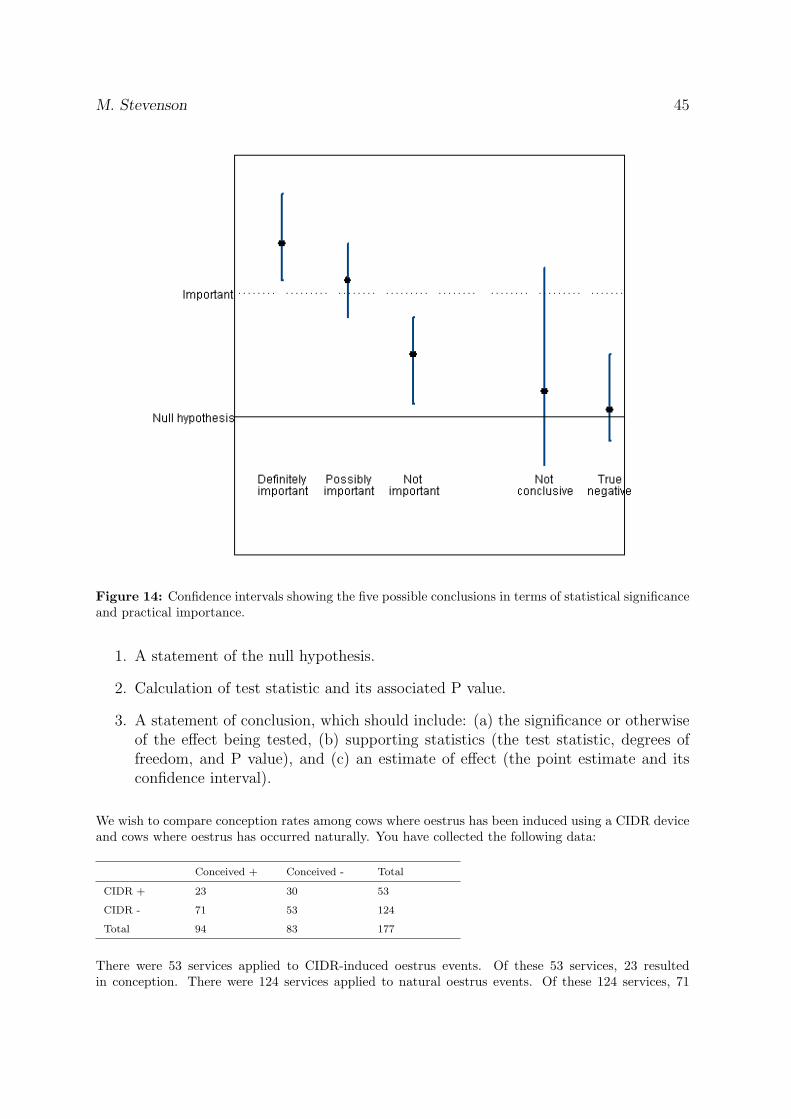
The five possibilities (as shown in Figure 14) are:

1. The difference is significant and certainly large enough to be of practical impor-tance — ‘definitely important’.

2. The difference is significant but it is unclear whether it is large enough to beimportant — ‘possibly important’.

3. The difference is significant but too small to be of practical importance — ‘notimportant’.

4. The difference is not significant but may be large enough to be important — ‘notconclusive’.

5. The difference is not significant and also not large enough to be of practical im-portance — ‘true negative’.

5.2 Steps involved in testing significance

The full answer to any exercise involving a significance test should include:

M. Stevenson 45

Figure 14: Confidence intervals showing the five possible conclusions in terms of statistical significanceand practical importance.

1. A statement of the null hypothesis.

2. Calculation of test statistic and its associated P value.

3. A statement of conclusion, which should include: (a) the significance or otherwiseof the effect being tested, (b) supporting statistics (the test statistic, degrees offreedom, and P value), and (c) an estimate of effect (the point estimate and itsconfidence interval).

We wish to compare conception rates among cows where oestrus has been induced using a CIDR deviceand cows where oestrus has occurred naturally. You have collected the following data:

Conceived + Conceived - Total

CIDR + 23 30 53

CIDR - 71 53 124

Total 94 83 177

There were 53 services applied to CIDR-induced oestrus events. Of these 53 services, 23 resultedin conception. There were 124 services applied to natural oestrus events. Of these 124 services, 71


resulted in conception. A chi-squared test will be used to compare the two proportions (that is, testthe hypothesis that 23/53 and 71/124 do not differ).

Null hypothesis: conception rates for CIDR-induced oestrus events are equal to conception rates fornatural oestrus events.

The chi-squared test statistic, calculated from these data is 2.86. The number of degrees of freedom is1. The P-value corresponding to this test statistic and degrees of freedom is 0.09.

We accept the accept the null hypothesis that conception rates for CIDR-induced oestrus events areequal to conception rates for natural oestrus events (chi-squared test statistic = 2.86, df = 1, P = 0.09).

The conception rate for CIDR-induced oestrus events was 43% (95% CI 31% to 57%). The conceptionrate for natural oestrus events was 57% (95% CI 48% to 66%).

M. Stevenson 47

6 Diagnostic tests


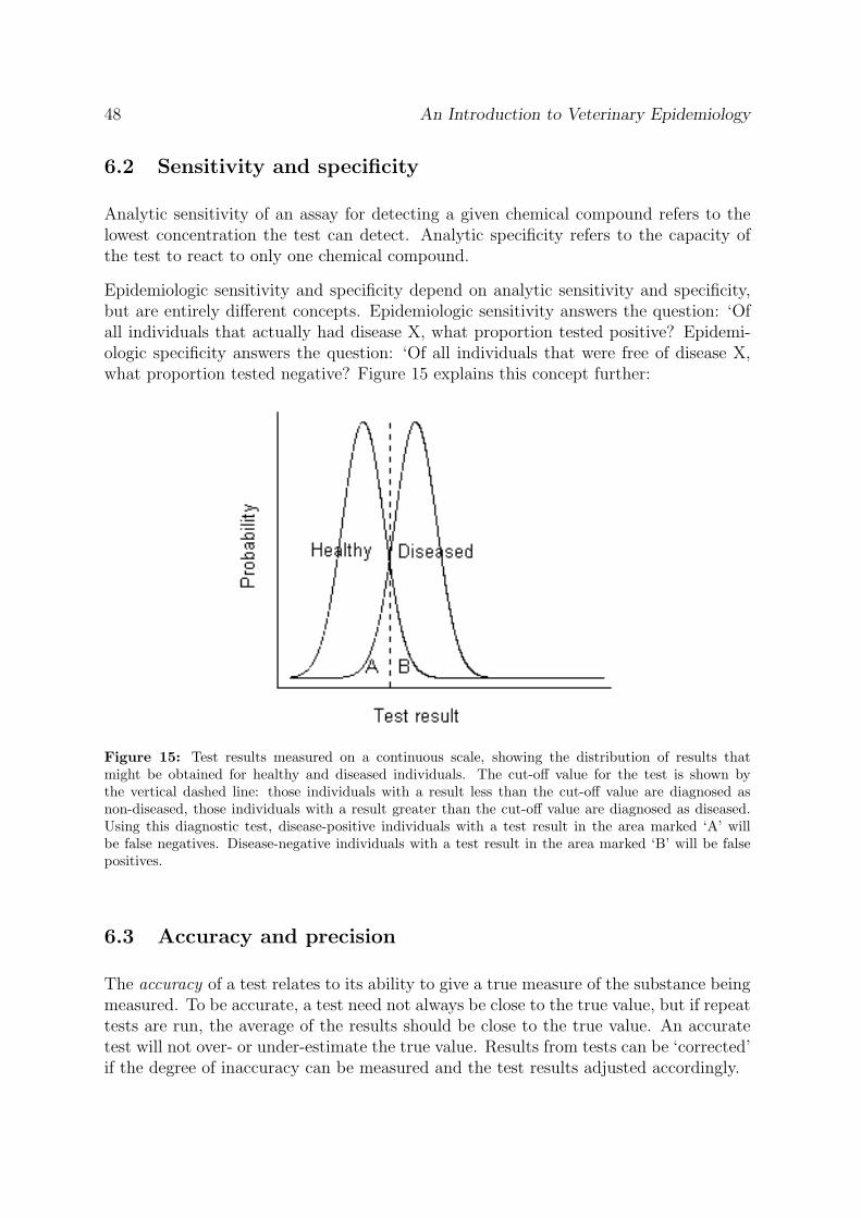
• Explain what is meant by the terms sensitivity and specificity, as applied to diag-nostic tests.

• Given testing results presented in a 2 × 2 table, evaluate a test in terms of itssensitivity, specificity, and the overall misclassification.

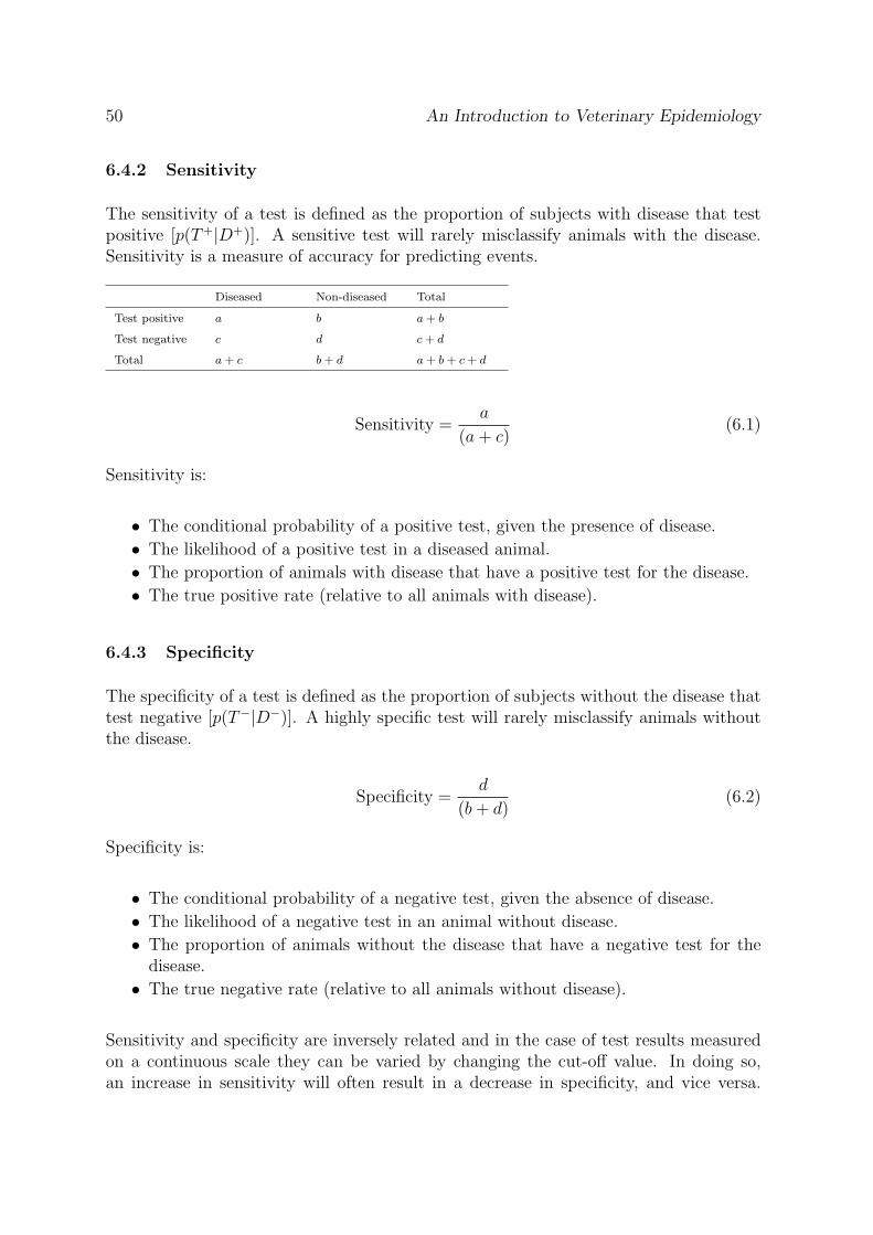
• Given testing results presented in a 2 × 2 table, calculate and interpret predictivevalues.

A test may be defined as any process or device designed to detect (or quantify) a sign,substance, tissue change, or body response in an animal. Tests included:

• Routine examination of an animal or premises.

• Questions posed during history taking.

• Clinical signs.

• Laboratory findings - haematology, serology, biochemistry, histopathology.

• Post mortem findings.

If tests are to be used in a decision-making context, the selection of an appropriate testshould be based on its ability to alter your assessment of the probability that a diseasedoes or does not exist.

6.1 Screening versus diagnosis

In clinical practice, tests tend to be used in two ways:

Screening tests are those applied to apparently healthy members of a population to detectseroprevalence of certain diseases, the presence or disease agents, or subclinical disease.Usually, those animals that return a positive to such tests are subject to further in-depthdiagnostic work-up, but in other cases (such as national disease control programs) theinitial test result is taken as the state of nature.

Diagnostic tests are used to confirm or classify disease status, provide a guide to selectionof treatment, or provide an aid to prognosis. In this setting, all animals are ‘abnormal’and the challenge is to identify the specific disease the animal in question has.


6.2 Sensitivity and specificity

Analytic sensitivity of an assay for detecting a given chemical compound refers to thelowest concentration the test can detect. Analytic specificity refers to the capacity ofthe test to react to only one chemical compound.

Epidemiologic sensitivity and specificity depend on analytic sensitivity and specificity,but are entirely different concepts. Epidemiologic sensitivity answers the question: ‘Ofall individuals that actually had disease X, what proportion tested positive? Epidemi-ologic specificity answers the question: ‘Of all individuals that were free of disease X,what proportion tested negative? Figure 15 explains this concept further:

Figure 15: Test results measured on a continuous scale, showing the distribution of results thatmight be obtained for healthy and diseased individuals. The cut-off value for the test is shown bythe vertical dashed line: those individuals with a result less than the cut-off value are diagnosed asnon-diseased, those individuals with a result greater than the cut-off value are diagnosed as diseased.Using this diagnostic test, disease-positive individuals with a test result in the area marked ‘A’ willbe false negatives. Disease-negative individuals with a test result in the area marked ‘B’ will be falsepositives.

6.3 Accuracy and precision

The accuracy of a test relates to its ability to give a true measure of the substance beingmeasured. To be accurate, a test need not always be close to the true value, but if repeattests are run, the average of the results should be close to the true value. An accuratetest will not over- or under-estimate the true value. Results from tests can be ‘corrected’if the degree of inaccuracy can be measured and the test results adjusted accordingly.

M. Stevenson 49

The precision of a test relates to how consistent the results of the test are. If a testalways gives the same value for a sample (regardless of whether or not it is the correctvalue), it is said to be precise.

6.3.1 Measuring accuracy

Assessment of test accuracy involves running the test on samples with a known quantityof substance present. These can be field samples for which the quantity of substancepresent has been determined by another, accepted reference procedure. Alternatively,the accuracy of a test can be determined by testing samples to which a known quantityof a substance has been added. The presence of ‘background’ levels of substance in theoriginal sample and the representativeness of these ‘spiked’ samples make this approachless desirable for evaluating tests designed for routine field use.

6.3.2 Measuring precision

Variability among test results might be due to variability among results obtained fromrunning the same sample within the same laboratory (repeatability) or variability be-tween laboratories (reproducibility). Regardless of what is being measured, evaluationof test precision involves testing the same sample multiple times within and/or amonglaboratories.

6.4 Test evaluation

The two key requirements of a diagnostic test are: (1) the test will detect diseasedanimals correctly, and (2) the test will detect non-diseased animals correctly.

6.4.1 The gold standard

A gold standard is a test or procedure that is absolutely accurate. It diagnoses alldiseased animals that are tested and misdiagnoses none.

In order to evaluate a new test we ideally need a gold standard. However, because ofpractical difficulties we often must accept a gold standard that is less than ‘absolutelyaccurate’. This can produce considerable difficulties in test evaluation and, as a result,statistical approaches have been developed to help estimate the two key characteristicsof tests (sensitivity and specificity) in the absence of a gold standard.


6.4.2 Sensitivity

The sensitivity of a test is defined as the proportion of subjects with disease that testpositive [p(T+|D+)]. A sensitive test will rarely misclassify animals with the disease.Sensitivity is a measure of accuracy for predicting events.


Test positive a b a + b

Test negative c d c + d

Total a + c b + d a + b + c + d

Sensitivity =a

(a + c)(6.1)

Sensitivity is:

• The conditional probability of a positive test, given the presence of disease.

• The likelihood of a positive test in a diseased animal.

• The proportion of animals with disease that have a positive test for the disease.

• The true positive rate (relative to all animals with disease).

6.4.3 Specificity

The specificity of a test is defined as the proportion of subjects without the disease thattest negative [p(T−|D−)]. A highly specific test will rarely misclassify animals withoutthe disease.

Specificity =d

(b + d)(6.2)

Specificity is:

• The conditional probability of a negative test, given the absence of disease.

• The likelihood of a negative test in an animal without disease.

• The proportion of animals without the disease that have a negative test for thedisease.

• The true negative rate (relative to all animals without disease).

Sensitivity and specificity are inversely related and in the case of test results measuredon a continuous scale they can be varied by changing the cut-off value. In doing so,an increase in sensitivity will often result in a decrease in specificity, and vice versa.

M. Stevenson 51

The optimum cut-off level depends on the diagnostic strategy. If the primary objectiveis to find diseased animals meaning false negatives are to be minimised and a limitednumber of false positives is acceptable, a test with a high sensitivity and good speci-ficity is required. If the objective is to make sure that every test positive is ‘truly’diseased (meaning no false positives, but limited amount of false negatives acceptable),the diagnostic test should have a high specificity and good sensitivity.

6.4.4 Positive predictive value

The positive predictive value is the proportion of subjects with postitive test resultswhich have the disease.

Positive predictive value =a

(a + b)(6.3)

Positive predictive value is:

• The predictive value of a positive test.

• The post test probability of disease following a positive test.

• The posterior probability of disease following a positive test.

6.4.5 Negative predictive value

The negative predictive value is the proportion of subjects with negative test resultswhich do not have the disease.

Negative predictive value =d

(c + d)(6.4)

Negative predictive value is:

• The predictive value of a negative test.

• The post test probability of no disease following a negative test.

• The posterior probability of no disease following a negative test.

Predictive values quantify the probability that a test result for a particular animalcorrectly identifies the condition of interest. Estimation of predictive values requiresknowledge of sensitivity, specificity and the prevalence of the disease in the population.It is important to remember that predictive values are used for interpretation at theindividual animal level and cannot be used to compare tests. The effect of prevalence onpredictive values is considerable. Given a prevalence of disease in a population of around


Figure 16: Relationship between prevalence and positive predictive value for tests of different sensi-tivities and specificities.

30% and we are using a test with 95% sensitivity and 90% specificity, the predictivevalue of a positive test would be 80% and the predictive value of a negative test wouldbe 98%. If prevalence of disease is only 3% and the test characteristics remain the same,the predictive value of a positive and negative test will be 23% and 99.8%, respectively.

Remember the following general rules about diagnostic tests:

• Sensitivity and specificity are generally independent of prevalence.

• If prevalence increases, positive predictive value increases and negative predictivevalue decreases.

• If prevalence decreases, positive predictive value decreases and negative predictivevalue increases.

• The more sensitive a test, the better its negative predictive value.

• The more specific a test, the better its positive predictive value.

6.5 Prevalence estimation

The estimate of disease prevalence determined on the basis of an imperfect test is calledthe apparent prevalence. Apparent prevalence is the proportion of all animals that givea positive test result. It can be more than, less than, or equal to the true prevalence. Ifsensitivity and specificity of a test are known, then true prevalence can be calculated.Take the following data:

In the example above, individual cow somatic cell counts (ICSCC) are used as a screeningtest for subclinical mastitis in dairy cattle. The threshold for a clinical diagnosis of

M. Stevenson 53

Mastitis + Mastitis - Total

High ICSCC 40 190 230

Low ICSCC 10 760 770

Total 50 950 1000

mastitis is an ICSCC of > 200 cells/mL. The apparent prevalence of mastitis in thisherd is (40 + 190) / 1000 = 23%. The true prevalence is (40 + 10) / 1000 = 5%.

An alternative (and perhaps more complicated) formula for estimating true prevalenceis:

p(D+) =AP − (1− Sp)

1− [(1− Sp) + (1− Se)]=

AP + Sp− 1

Se + Sp− 1(6.5)

Where:

AP : apparent prevalenceSe: sensitivity (0 - 1)Sp: specificity (0 - 1)

On the basis of the data presented above, true prevalence p(D+) may be calculated as follows:

AP = 0.23Se = 0.80Sp = 0.80

p(D+) = (0.23 + 0.80 - 1) / (0.80 + 0.80 - 1)p(D+) = 0.03 / 0.6p(D+) = 0.05

This approach is useful when all we know is the sensitivity and specificity of the diagnostic test we areusing and the apparent prevalence.

6.6 Diagnostic strategies

Clinicians commonly perform multiple tests to increase their confidence that a patienthas a particular diagnosis. When multiple tests are performed and all are positive, theinterpretation is straightforward: the probability of disease being present is relativelyhigh. It is far more likely however, that some of the tests return a positive result andothers will be negative. Interpretation, in this case, is more complicated.

Multiple test results can be interpreted in parallel or series.


6.6.1 Parallel interpretation

Parallel interpretation means that when multiple tests are run an individual is declaredpositive if at least one of the multiple tests returns a positive result. Interpreting testresults in parallel increases the sensitivity and therefore the negative predictive valuefor a given disease prevalence. However, specificity and positive predictive value arelowered. As a consequence, if a large number of tests are performed and interpreted inthis way then virtually every individual will be considered ‘positive’.

6.6.2 Serial interpretation

Series interpretation means that when multiple tests are run an individual is declaredpositive if all tests return a positive result. Series interpretation maximises specificityand positive predictive value which means that more confidence can be attributed topositive results. It reduces sensitivity and negative predictive value, and therefore itbecomes more likely that diseased animals are being missed.

6.6.3 Screening and confirmatory testing

With a screening and confirmatory test strategy (as often used in a disease controlscheme) a screening test is applied to every animal in the population to ‘screen’ thepopulation for positives. Ideally, this test should be easy to apply and at low cost. Italso should be a highly sensitive test so that it misses only a small number of diseasedor infected animals. Its specificity should still be reasonable, so that the number of falsepositives subjected to the confirmatory test remains economically justifiable.

Individuals that return a negative result to the screening test are considered definitivenegatives and not submitted to any further examination. Any positive screening testresult is subjected to a confirmatory test. The confirmatory test can require moretechnical expertise and more sophisticated equipment, and be more expensive, becauseit is only applied to a reduced number of samples. But it has to be highly specific, andany positive reaction to the confirmatory test is considered a definitive positive.

The same principles apply to disease control and eradication schemes. We firstly apply atest to detect disease: individuals identified as positive are removed from the population.To efficiently identify positives we need a highly sensitive test. During this early phaseof a program the apparent prevalence will be higher than the true prevalence, as aconsequence of test specificity being less than 100%. As the program continues, testpositive animals are identified and culled. Population prevalence of disease declines. Asprevalence declines, the positive predictive value of testing declines which increases thegap between apparent and true prevalence. The proportion of false positives will thenincrease. At this stage a highly specific test is required. In some cases it may becomenecessary to use a number of tests interpreted in series to increase specificity.

Rules of thumb:

M. Stevenson 55

• If the objective is to find disease (e.g. diagnose neoplasia early in a much-lovedpet) use a highly sensitive test.

• If the objective is to confirm the absence of disease (e.g. testing a cow for brucellosisbefore it is imported into New Zealand) use a highly specific test.

6.6.4 Batteries of multiple tests

Running ‘batteries’ of multiple tests is common in clinical practice. Blood samplesfrom patients are sent to a laboratory and for a fixed fee a range of haematological andbiochemical analyses are performed. The objective is to identify normal and abnormalblood parameters. The technique becomes useful, if a set of different parameters is ofdiagnostic value for establishing a pattern which is suggestive of a particular disease. Theapproach becomes questionable, if it is part of a ‘fishing expedition’ for a diagnosis. Weneed to keep in mind that a cut-off for a single test is typically set such that it includes95% of the normal population, which means the test will produce 5% false positives.As an example, with 12 diagnostic tests measuring different blood parameters, each ofthem will have a 0.95 probability of diagnosing a ‘normal’ animal correctly as negative.But it also means that the overall chance of a correct negative diagnosis on all tests is0.912 = 54%. There is, as a result, a 46% chance that a ‘normal’ animal has at least oneabnormal (false positive) value among the 12 tests.

6.6.5 Likelihood ratios

Diagnostic testing is often undertaken to help us decide whether or not an individualis diseased. Because diagnostic tests are imperfect (that is, false positives and falsenegatives occur) clinicians need to move away from the ‘test positive = disease positive’,‘test negative = disease negative’ paradigm and think about testing as a process thatmodifies our prior probability estimate that disease is present into a posterior probabilityestimate. Likelihood ratios offer a means for doing this.

The likelihood ratio for a positive test is estimated on the basis of dividing the probabilityof a particular test result in the presence of disease (sensitivity) by the probability ofthe test result in the absence of disease (1 - specificity). The result is interpreted ashow likely it is to find a positive test result in a diseased individual compared withnon diseased individuals. The likelihood ratio for a negative test equals (1 - sensitivity)divided by the specificity. Thus:

LR+ =Se

1− Sp(6.6)

LR− =1− Se

Sp(6.7)


Where:

Se: sensitivity (0 - 1)Sp: specificity (0 - 1)

Likelihood ratios (LR) can be calculated using single cut-off values, so that one obtainsonly one pair of likelihood ratios, one for a positive (LR+) and another for a negativetest result (LR-). More powerful information can be extracted from the diagnostic testby using multilevel likelihood ratios. In this case every test value, or more often severalranges of test values, will have a specific LR+ and LR-. The advantage of the multilevellikelihood ratio method is that it allows the clinician to take account of the degree ofabnormality, rather than just use crude categories such as presence or absence of disease.

Likelihood ratios provide a quantitative measure of the diagnostic information containedin a particular test result. If we consider the expectation of the likelihood that ananimal has a certain condition (= pre-test odds of disease) the likelihood ratio of thetest multiplied by the pre-test odds gives us a revised estimate of the odds of disease (=post-test odds). This result can be re-expressed as a probability (rather than an odds)to make it more interpretable. To convert odds to probability and vice versa, we use thefollowing equations:

Odds of event =Probability of event

1 - Probability of event(6.8)

Probability of event =Odds of event

1 + Odds of event(6.9)

Individual cow somatic cell counts (ICSCC) are used as a screening test for sub-clinical mastitis in dairyherds. A client has a herd of dairy cows where the prevalence of subclinical mastitis is estimated to bearound 5%. You receive the following data from herd testing:

Mastitis + Mastitis - Total

ICSCC > 200 40 190 230

ICSCC < 200 10 760 770

Total 50 950 1000

At a later date you examine an individual cow from this herd and note that she has an ICSCC of320,000 cells/mL. What is the probability that she has mastitis?

Using a fixed ICSCC threshold 200,000 cells/mL to classify individuals as mastitic or not, and assumingthat ICSCC testing has a sensitivity of 80% and a specificity of 80%, the calculated positive predictivevalue is 40 ÷ 230 = 17%. On the basis of these calculations we reckon that if a cow has an ICSCCvalue greater than 200,000 cell/mL the probability that she really has mastitis is around 17%.

Using the likelihood ratio method likelihood ratios for categories of ICSCC values can be calculated:

The posterior probability of mastitis is determined as follows:

M. Stevenson 57

ICSCC < 100 100 – 200 200 – 300 300 – 400 > 400

LR (+) 0.14 0.37 2.50 14.50 40.80

1. The pre-test probability of mastitis is 0.05.

2. The pre-test odds of mastitis: 0.05 / (1 - 0.05) = 0.053.

3. The post-test odds of mastitis given a positive test result: pre-test odds × LR(+) = 0.053 × 14.5 =0.76.

4. The post-test probability of mastitis given a positive test result: 0.76 / (1 - 0.76) = 0.43.

The post-test probability of a cow with a ICSCC of 320,000 cells/mL being mastitic is around 43%.

Post-test probabilities can be quickly determined in practice by using a nomogram, asshown in Figure 17. On the left hand side of the nomogram (labelled ‘pre-test probabil-ity’) we mark the pre-test probability that the individual being examined has disease.We next identify the point defining the likelihood ratio of a positive test result alongthe middle scale. Finally, we draw a straight line from the pre-test probability estimatethrough the likelihood ratio value to the corresponding post-test probability value onthe right-hand side of the chart.

A nice feature of this approach to evaluating test information is that sequential testingcan be easily handled. If we are using serial interpretation, the post-test probability ofdisease from the first test becomes the pre-test probability for the second test:

To continue the mastitis example described above lets imagine that we clinically examine our cow andas part of that examination we test milk from each quarter using a rapid mastitis test (RMT). We aretold that the sensitivity and specificity of the RMT is 70% and 80%, respectively. Our cow returns apositive result to the RMT. What now is her post-test probability of disease?

Given the test characteristics of the RMT, the likelihood ratio of a positive test is 3.5 (= 0.7 / 1 - 0.80).If the pre-test probability of disease is 0.43 we can use a nomogram to estimate the posterior probabilityof disease, given a positive test, to be 0.72. We are now much more certain that this cow has mastitis.

The advantage of the nomogram method is that we can better appreciate the ‘value’ (i.e. the increasein post-test probability) provided by each diagnostic test that is applied (in the above example, ICSCCprovided more information to use compared with the RMT). If the cost of each test applied is knownthe ‘cost per unit increase in post-test probability’ can be determined, enabling us to be more objectivein our use of diagnostic resources.


Figure 17: Nomogram for post-test probability calculations using likelihood ratios of a positive testresult.

Figure 18: Diagram showing how the estimated probability of disease changes after applying a seriesof diagnostic tests. In our example of the cow with mastitis, we had a prior belief that the probability ofthe cow being mastitic was 5%. After considering the ICSCC result this probability increased to 43%.After applying a rapid mastitis test and getting a positive result, the probability of the cow havingmastitis increased to 72%.

M. Stevenson 59

7 Sampling populations


• Explain the key features of simple random sampling, systematic random sampling,stratified random sampling, and cluster sampling.

• Describe the advantages of disadvantages of simple random sampling, systematicrandom sampling, stratified random sampling, and cluster sampling.

• Describe ways to reduce error when making inferences from sampled data.

Epidemiologists frequently examine populations to:

• Detect the presence of a disease;

• Demonstrate that a disease is not present within a population; and

• Establish the level of occurrence of a disease within a population.

To produce accurate estimates of disease we must be able to measure populations effec-tively. The exact level of disease within a population will be obtained if every individualwithin the population is examined (and if there was no measurement error). This tech-nique is a census. However, in many situations a census is impossible and/or excessivelyexpensive. Usually an accurate estimate can be obtained by examining some of theanimals (a sample) from the population.

7.1 Probability sampling methods

7.1.1 Simple random sampling

Simple random sampling occurs when each subject in the population has an equal chanceof being chosen.

Figure 19: Simple random sampling. If a sample of five cows was required, five random numbersbetween 1 and 10 would be generated and cows selected on the basis of the generated random numbers.


7.1.2 Systematic random sampling

With systematic random sampling, the selection of sampling units occurs at a predefinedequal interval. This process is frequently used when the total number of samplingunits is unknown at the time of sampling (e.g. in a study where patients that enter anemergency department of a hospital on a given day are to be sampled — at the startof the study day we do not know the total number of patients seen by the end of the day).

Suppose we are studying inpatient medical records on an ongoing basis for a detailed audit. The totalnumber of records in the population is not likely to be known in advance of the sampling since therecords are to be sampled on an ongoing basis (and so it would not be possible to use simple randomsampling). However, it would be possible to guess the approximate number of records that would beavailable per time period and to select a sample of one in every k records as they become available.

We require a total of 300 records over a 12-month period to complete the study. If there are, on average,ten new discharge records available per day then total number of records available per year is estimatedto be 10 × 365 = 3650. To obtain the required number of records per year in the sample, the samplinginterval k should be the largest integer in the quotient 3650 ÷ 300. Since the value of the quotient is12.17, the sampling interval k would be 12. Thus, we would take a sample of 1 from every 12 records.

One way to implement this procedure is to identify each record as it is created with a consecutivenumber. At the beginning of the study a random number between 1 and 12 is chosen as the startingpoint. Then, that record and every twelfth record beyond it is sampled. If the random number chosenis 4, then the records in the sample would be 4, 16, 28, 40, 52, and so on.

7.1.3 Stratified random sampling

Stratified sampling occurs when the sampling frame is divided into groups (strata)and a random selection within each stratum are selected. Stratified sampling isfrequently undertaken to ensure that there is adequate representation of all groups inthe population in the final sample.

Suppose that you wish to determine the prevalence of disease in the pig population of a region.Previous surveys have indicated that 70% of the region’s pigs are located in very large, intensivespecialised pig farms, 20% of pigs are found within smaller farming units (frequently as a secondaryenterprise on large dairy farms), and 10% of pigs are kept singly within small plots around towns (bypeople whose major occupation is not farming). With proportional stratification, a sample would beselected at random from within each stratum such that the aggregated sample would consist of 70%pigs obtained from the large intensive farms, 20% pigs obtained from the smaller pig farms, and 10%pigs obtained from small plots near towns.

In some situations obtaining a sample from a particular stratum is more difficult or costlythan for other strata. In the example described it may be more costly to sample from

M. Stevenson 61

the pigs held in small plots around towns. This may be due to an incomplete registerof smallholdings, difficulties in contacting pig owners and arranging suitable times tovisit and perhaps extra travel requirements. In this situation, a technique known asnon-proportional sampling may adopted.

An advantage of stratified sampling is that the precision of parameter estimates isimproved. If the population can be divided into logical strata whereby the variationwithin each stratum is small compared with the variation between strata a more preciseestimate will be obtained.

We wish to determine average total lactation milk volume (total litres) produced by dairy cows in aregion. The region contains two breeds of cattle. One breed (Friesian) is characterised by production oflarge volumes of milk with low concentrations of milk solids. The other breed (Jersey) is characterisedby production of small volumes of milk with high concentrations of milk solids. By dividing the popula-tion into breed strata and sampling within each stratum, the average lactation milk volume productionof each breed can be estimated with accuracy. The mean milk production for cows within the region canalso be estimated by calculation of a weighted mean based upon each stratum mean and the stratum size.

Figure 20: Stratified random sampling. A group of animals are stratified by breed and a randomsample within each breed taken.

7.1.4 Cluster sampling

Cluster sampling occurs when the sampling frame is divided into logical aggregations(clusters) and a random selection of clusters is performed. The individual sampling units


within the selected clusters are then examined. Clustering may occur in space or time.For example, a litter of piglets is a cluster formed within a sow, a herd of dairy cows isa cluster within a farm, and a fleet of fishing boats is a cluster formed within a port orharbour.

• One-stage cluster sampling occurs when all sampling units within the selectedclusters are examined.

• Two-stage cluster sampling occurs when a random selection of sampling unitswithin the randomly selected clusters is examined. The primary sampling units arethe clusters and the secondary sampling units are the individual units of interest.

Cluster sampling is frequently required when a sampling frame of individual unitscannot be produced. Instead, a sampling frame of clusters is used to access theindividual units. Clusters of individuals tend to form for logical reasons (for example,litters, villages). Individuals within a cluster tend to be more alike than individualsfrom other clusters. This observation frequently results in the variation between clustersbeing greater than the variation within clusters.

Suppose that you wish to conduct a survey to determine if overfishing of any species of ocean fish isoccurring within a country. There is no registration requirement to fish in this country, so a samplingframe of individual people who fish cannot be drawn. However, all ocean-going fishing boats must bebased at deep harbours. A study of a map of the country indicates that there are 30 deep harbourscapable of supporting ocean-fishing vessels. A random selection of harbours is made. All the fishingboats moored within each selected harbour are identified and listed. A random selection of boats ismade and the catch from each boat is examined on a designated day. The quantity of each fish speciespresent on each boat is estimated. This is used to provide an estimate of the total fishing pressure foreach species of interest.

7.2 Non-probability sampling

Non-probability sampling occurs when the probability of selection of an individual withina population is not known and some groups within the population are more or less likelythan other groups to be selected. Non-probability sampling includes:

• Convenience sampling: where the most accessible or amenable sampling units areselected;

• Purposive sampling: where the most desired sampling units are selected; and

• Haphazard sampling: where sampling units are selected using no particular schemeor method. Inherent in this type of sampling is the problem that subconsciousforces may influence the person selecting the units in an attempt to ‘balance’ thesample. For example, a young animal may be preferred for the next selectionimmediately after an older animal has been selected.

M. Stevenson 63

Non-probability sampling will produce biased population estimates, and the extent ofthat bias cannot be quantified.

7.3 Sources of error in sample estimates and how to reduceerror

When you derive an estimate from a sample you want it to be precise and accurate.A precise estimate has confidence intervals that are small. An accurate has confidenceintervals that are centred on the true population value. There are two types of errorthat can exist within a sample estimate: random errors and bias. The difference betweenrandom error and bias may be explained using the following diagram:

Figure 21: The distribution of bullets fired at the target on the left show little evidence of randomerror and bias. The distribution of the bullets fired at the centre target show a high degree of randomerror and a low degree of bias. The distribution of the bullets fired at the target on the right show alow degree of random error and a high degree of bias.

There are two types of error that can exist within a sample estimate:

7.3.1 Random error

Random error is caused by chance. A random selection of individuals taken to make upa sample will differ slightly from each other. These differences will result in sample esti-mates that differ slightly from each other and also from the target population. Randomerror is the inherent error that arises from using a sample to make a measurement of apopulation. The influence of random error may be reduced by:

1. Increasing the size of the sample taken.

2. Modifying the selection procedure to ensure that only the target group is sampled.

3. Using an appropriate scale of measurement.

7.3.2 Bias

Bias is caused by systematic error, a systematic error being one that is inherent tothe technique being used that results in a predictable and repeatable error for eachobservation. Bias may present itself in two ways:


1. Non-observational errors are due to inappropriate sample selection. These errorsmay arise from failure to include an important group of individuals within thesampling frame (resulting in their exclusion from selection), or as a result of missingdata. In some situations data may be missing from a particular group of individualswithin the sample.

2. Observational errors are due to inappropriate measurements. These may be at-tributable to false responses (i.e. participants make untrue statements) or to mea-surement errors.

7.4 Common sampling methods

Random sampling means that each unit of interest within the population has the sameprobability of selection into the sample as every other unit. The probability of selectionof individual units must not differ. This is irrespective of accessibility, ease of collectionor other differences that may exist between individuals.

7.4.1 Methods of randomisation

There are two principal techniques for random sampling, physical randomisation andthe use of random numbers.

Physical randomisation is a process where sampling units are selected using physicalsystems that contain random elements. These include the selection of numbered marblesfrom a bag, the use of a die, or the toss of a coin.

Random numbers are a sequence of numbers comprising individual digits with an equalchance that any number from 0 to 9 will be present. Tables of random numbers canbe used for sample selection. Some computer programs can generate random numbers.These programs use algorithms to produce the sequence of numbers. The sequence ofnumbers that is generated depends upon the value chosen as the starting value for thealgorithm (the seed value). Whilst there is an equal probability that any digit from 0to 9 will be present in a position chosen at random from the sequence, the actual digitpresent at each point of the sequence is determined by the seed value. In other words,the exact sequence of random numbers can be reproduced if the process is repeatedusing the same seed value. Computer-generated random numbers are frequently calledpseudo-random numbers for this reason.

7.4.2 Replacement

Samples may be taken in one of two ways: sampling with replacement or samplingwithout replacement.

M. Stevenson 65

In sampling with replacement, each selected unit is examined and recorded and thenreturned to the sampling frame. These units may then be selected into the sampleagain.

In sampling without replacement, each selected unit is examined and recorded and thenwithdrawn from the sampling frame. These units are excluded from selection into thesample again.

7.5 Taking a sample of the appropriate size

7.5.1 Simple random sampling

The following formulae may be used to approximate sample sizes appropriate to estimatepopulation parameters (population total, mean, and proportion) on the basis of a simplerandom sample. From: Levy and Lemeshow (1999) p 74.

Total:n >4V 2

x

ε2(7.1)

Mean:n >4V 2

x

ε2(7.2)

Proportion:n >4(1− Py)Py

ε2(7.3)

Where:V 2

x : the relative variance (the estimated population variance divided by the square ofthe estimated population mean)ε: the maximum relative difference between our estimate and the unknown populationvaluePy: the unknown population proportion

Suppose that a survey of retail pharmacies is to be conducted. The purpose of the survey is to estimatethe average retail price of 20 tablets of a commonly used vasodilator. An estimate is needed that iswithin 10% of the true value of the average retail price in the state. Data collected earlier on 1000pharmacies in another state indicates an average price of $7.00 with a standard deviation of $1.40. Howmany pharmacies should be included in the survey to be 95% confident that the surveyed value will bewith 10% of the average retail price in the state?

Data from the earlier survey can be used to estimate relative variance:

The estimated population variance = 1.40 × 1.40 = 1.96The estimated population mean is 7.00V 2 = 1.96 / (7 × 7) = 0.04Sample size = (4 × 0.04) / (0.1 × 0.1) = 16


A sample of 16 pharmacies are required to meet the requirements of the survey.

7.5.2 Proving freedom from disease

Veterinarians are frequently asked to test groups of animals to confirm the absenceof disease. How do we determine the number of animals that should be tested beforewe can be 95% confident that disease does not exist within the population? The ‘ruleof three’ provides a ballpark estimate. The rule of three states that the number ofindividuals that need to be tested equals 300 divided by the prevalence (expressed as apercentage).

What is the approximate number of individuals that should be tested to confirm freedom if the expectedprevalence of disease in a population is 25%?

A minimum of (300 ÷ 25) = 12 individuals should be tested.

The probability of failing to detect disease (when it actually exists) is given by:

p = (1− d

N)n (7.4)

Where:N : the population sized: the number of diseased animals presentn: number of animals tested

We estimate the prevalence of brucellosis in a herd of 200 to be around 5%. What is the probability offailing to detect brucellosis if we test 28 animals?

d = 0.05 × 200 = 10N = 200n = 28p = (1− 10/200)28 = 0.23

There is a 23% chance that we will fail to detect disease if we sample 28 cattle from a herd of 200.

7.6 Estimation of the proportion of diseased animals in a pop-ulation

It is often desired to estimate the prevalence of a disease in a population on the basis ofa screening test that has less than perfect sensitivity or specificity.

M. Stevenson 67

The screening test is usually a test that is inexpensive and feasible to use in the fieldin comparison to a more accurate diagnostic test which, although available, would notbe feasible to use in a survey situation. The major objectives of screening programs areto identify for subsequent intervention individuals having a condition or disease, andthe major statistical issues involve the evaluation of the likelihood that an individualscreened as positive really has the disease and that an individual screened as negativereally does not have the disease.

The basic methodology involves taking a sample of n individuals from a population of Nindividuals and giving the screening test to each of the sampled individuals. Apparentprevalence can then be calculated, and if sensitivity and specificity of the test are known,the maximum likelihood estimate of the proportion of the population that are diseasepositive p(D+) can be calculated:

p(D+) =AP − (1− Sp)

1− [(1− Sp) + (1− Se)]=

AP + Sp− 1

Se + Sp− 1(7.5)

Where:

AP : apparent prevalenceSe: sensitivity (0 - 1)Sp: specificity (0 - 1)

Suppose we take a simple random sample of 150 cows from a herd of 2560. Each cow is given a screeningtest for brucellosis which has a sensitivity of 96% and a specificity of 89%. Of the 150 cows tested, 23were positive to the screening test. What is the estimated prevalence of brucellosis in this herd?

AP = 23 / 150 = 0.15Se = 0.96Sp = 0.89

p(D+) = (0.15 + 0.89 - 1) / (0.96 + 0.89 - 1)p(D+) = 0.040 / 0.850p(D+) = 0.051

The estimated prevalence of brucellosis in this herd is 5.1 cases per 100 cows.


8 Outbreak investigation


• Describe the steps to take during an outbreak investigation, including descriptionof the outbreak by animal, place and time.

An outbreak is a series of disease events clustered in time. During an outbreak theinvestigator asks the questions:

• What is the problem?

• Can something be done to control it?

• Can future occurrences be prevented?

These notes outline an approach to investigating outbreaks of disease in animal popu-lations. Although the term outbreak implies a sudden (and possibly spectacular) event(e.g. an outbreak of botulism in feedlot cattle), be aware that outbreaks can be of amore insidious nature: some causing subclinical losses in a population of animals overan extended period before being identified, characterised and investigated.

8.1 Verify the outbreak

8.1.1 What is the illness?

Once a suspected outbreak is identified, identifying the specific nature of the illness isan important early step. An attempt should be made to characterise cases (leadingtowards a formal case definition, see below). Usually it will not be possible to make adefinitive diagnosis at this stage. What is required is a ‘working definition’ of the diseaseor syndrome: for example ‘ill thrift in recently weaned calves’ or ‘sudden death in growerpigs’.

8.1.2 Is there a true excess of disease?

The first issue to be certain of is whether or not the outbreak is genuinely an unusualevent worthy of special attention. The number of cases per unit time should be sub-stantially greater than what is ‘normal’ for the group of individuals under investigation.It is common to have owners and others concerned about a possible outbreak which istransient increase in the normal level of endemic disease.

M. Stevenson 69

8.2 Investigating an outbreak

8.2.1 Establish a case definition

A case definition is the operational definition of a disease for study purposes. A goodcase definition has two parts: (1) it specifies characteristics shared by all members ofthe class being defined, and (2) it specifies what distinguishes them from all outside theclass. Collect historical data and examine affected individuals to establish the principalfeatures which they share in common. These form the case definition.

8.2.2 Enhance surveillance

When it is suspected that an outbreak is occurring, enhanced surveillance can be useful toidentify additional cases. Enhanced surveillance may involve both heightening awarenessto increase passive case reports and implementing targeted surveillance. Techniquesinclude directly contacting field practitioners by telephone, facsimile or email, via healthdepartment web pages and email discussion groups. For large outbreaks media releases(print, television, radio) are extremely effective.

8.2.3 Describe outbreak according to individual, place and time

Collect historical, clinical and productivity data on those individuals that are affected(cases) and those that are not affected. It is a mistake to concentrate exclusively ondiseased animals. If possible, all cases of diseased animals should be included in theinvestigation. If there are large numbers of unaffected individuals (controls) you may se-lect a representative sample of unaffected individuals for examination. You may considermatching controls with some characteristic of the cases e.g. age and gender.

Plot an epidemic curve by identifying the first case (index case) and then graphingsubsequent numbers of cases per day or per week from the index case through to theend of the outbreak. An extremely rapid increase in the number of cases from theindex case suggests a common source epidemic (all the diseased animals were exposedto the source at about the same time). If the number of disease animals is increasingover time, this is more indicative of a propagated epidemic which is more typical ofcontagious disease or prolonged exposure to the agent via vectors or toxins.

Location is often an important risk factor for disease. Draw a sketch map of the area orthe layout of the pens and the number of cases within pens. This includes examinationof animal movements and recent additions to the herd or flock. The investigator shouldinspect the drawing for possible interrelationships among cases, and between location ofcases and other physical features.


8.2.4 Develop hypotheses about the nature of exposure

At this stage, you will probably have some suspicions about what has caused the outbreak— that is, you will have started to form some hypotheses. Your next job is to test thesehypotheses using the various analytical techniques described below.

8.2.5 Conduct analytical studies

Part of the data collection procedure above will have entailed collecting individual-leveldetails such as age, sex, breed, date of parturition, stage of production. Individualsshould be categorised according to the presence of each attribute. This data can bepresented as frequency and attack rate tables. As part of the analysis, relative riskestimates can be computed for each of the potential risk factors. The objective is toidentify the highest as well as the lowest risks for disease. The objective is to demonstratethat an observed association is not due to chance. The result from this analysis should bea working hypothesis taking into account potential causes, sources, mode of transmission,exposure period and the population at risk.

8.3 Implement disease control interventions

At this stage it may be possible to produce a hypothesis regarding the cause of theoutbreak. If further investigation is warranted then other epidemiological studies (case-control, prospective cohort etc) may be designed and implemented. You may also usemore complex analytical techniques to analyse data already collected (multivariate tech-niques).

M. Stevenson 71

9 Appraising the literature


• Describe, in your own words, the four main areas that should be considered whenappraising the scientific literature.

Reading the literature is necessary to keep up to date with new developments and tolearn more about a particular area of science that interests us.

Fortunately, there appears to be no shortage of literature available to read, and ourability to source this literature easily has been facilitated by the Internet (either inthe form of peer-reviewed articles published on-line by established journals or as ’pre-print’ publications published by individuals on their own web pages). Although the‘freedom’ of the Internet allows information to be widely disseminated, the quality ofthat information varies widely. As a result, as good scientists, we need to be discerningabout what we read and (more importantly) what we believe. A systematic method ofappraising (or evaluating) the literature helps us to do this. We describe a systematicapproach to appraising the epidemiological literature, which consists of:

• Describing the evidence,

• Assessing the internal validity of the study,

• Assessing the external validity of the study, and

• Comparing the results with other available evidence.

9.1 Description of the evidence

The first step in evaluating a scientific article is to understand exactly what relationshipwas being evaluated and what hypothesis was being tested. The reader should be ableto identify the exposure variable(s) and the outcome variable. It is also necessary tocategorise the study in terms of its design (survey, case-control, observational cohort,intervention cohort). Definition of the subjects that were studied in terms of sourcepopulations, the eligibility criteria, and the participation rates of the different groupsthat are being compared.

Having defined the topic of study, it is then useful to summarise the main result - whatis the result in terms of the association between exposure and outcome? It should bepossible to express the main result in a simple table and obtain from the paper the meansto calculate the appropriate measure of association (relative risk, odds ratio, differencein proportions) and the appropriate test of statistical significance.


9.2 Internal validity - non-causal explanations

Having described the study the next step is to assess its internal validity — that is, forthe subjects who were studied, does the evidence support a causal relationship betweenthe exposure and the outcome? We consider the three possible non-causal mechanismswhich could produce the observed results:

• Are the results likely to be affected by observation bias?

• Are the results likely to be affected by confounding?

• Are the results likely to be affected by chance variation?

It is useful to consider each of these aspects separately. The order of these non-causalexplanations is important. If there is severe observation bias, no analytical manipulationof the data will overcome the problem. If there is confounding, then appropriate analysiswill (in most cases) overcome the problem. The assessment of chance variation should bemade on the main result of the study, after considering issues of bias and confounding.

9.3 Internal validity - positive features of causation

9.3.1 Is there a correct temporal relationship?

For a relationship to be causal, the putative exposure must act before the outcomeoccurs. In a prospective study design where exposed and non-exposed subjects arecompared, this requirement is established by ensuring that subjects do not already havethe outcome of interest when the study starts. The ability to clarify time relationshipsis weaker in retrospective studies, and care is required to ensure that possible causalfactors did in fact occur before the outcome of interest.

A difficulty in all study designs, but more so in retrospective studies, is that the oc-currence in biological terms of the outcome of interest may precede the recognition anddocumentation of that outcome by a long and variable period of time (e.g. some cancers).

9.3.2 Is the relationship strong?

A stronger association, that is a larger relative risk, is more likely to reflect a causalrelationship. As a measured factor gets closer to a biological event on the causal path-way, the relative risks become larger. The fact that a relationship is strong does notprotect us against certain non-causal relationships, however if the relationship that isobserved is due to bias, then the bias must be large and therefore easy to identify. If astrong relationship is due to confounding, either the association of the exposure with theconfounder must be very close, or the association of the confounder with the outcomemust be very strong.

M. Stevenson 73

9.3.3 Is there a dose-response relationship?

In some circumstances the demonstration of a smooth dose-response relationship maybe a strong argument against an identified relationship arising as a result of bias. Ingeneral, we should expect uni-directional dose-effect relationships and evidence that thisis not the case should be considered carefully.

9.3.4 Consistency of the association

A causal relationship will be expected to apply across a wide range of subjects. An asso-ciation identified in one study that is consistent with the same association identified in adifferent groups of subjects is supportive of causation. The difficulty with consistency isthat very large data sets are required to assess the similarity or otherwise of associationsin different subgroups of subjects. Even with adequate numbers, the subgroups to becompared need to be defined on a priori grounds.

9.3.5 Specificity of association

It has been argued that a specific association between one causal factor and oneoutcome, is good evidence for causality.

An argument against the negative health effects of smoking arose from the observation that smokingwas shown to be associated with the occurrence of a number of cancers and other serious diseasesand therefore demonstrated non-specificity of action, making the hypothesis of a causal link with lungcancer less likely.

Specificity may be useful, if we do not make it an absolute criterion, as one causalagent may in truth produce various outcomes, and one outcome may result from variousagents. The concept is often useful in study design: as a check on response bias we maydeliberately collect information on factors which we expect to be the same in groupsthat we are comparing (similar results across groups will indicate a lack of observationbias).

9.4 External validity - generalisation of the results

If the internal validity of a study is poor, then there is no point in proceeding further— if the results are not valid for the subjects that were studied, its application to othergroups of subjects is irrelevant.


9.4.1 Can the results be applied to the eligible population?

The relationship between the study participants (those that participated in the study)and the population of eligible subjects (those that met the study inclusion criteria butdid not take part) should be well documented. Losses due to non-participation haveto be considered carefully as they are likely to be non-random, and the reasons for thelosses may be related to the exposure or the outcome.

9.4.2 Can the results be applied to the source population?

The important issue is not whether the subjects studied are ‘typical’, but whether theassociation between outcome and exposure given by the study participants is likely toapply to other groups. In assessing this applicability, we need to be specific about thefactors which are likely to affect the association.

Most clinical trials are done on patients in teaching hospitals. If a new therapy for a particular typeof neoplasia is shown to be effective in such a trial, we would readily apply the results to patients in adistrict hospital who had a similar stage and type of tumour and were of similar age, even though thetrial patients cannot be said to be representative of district hospital patients in a general or statisticalsense.

9.4.3 Can the results be applied to other relevant populations?

In general, the difficulties of applying results from one groups of subjects to another willbe minimal for issues of basic physiology and maximal for effects in which cultural andpsycho-social aspects are dominant.

9.5 Comparison of the results with other evidence

For many clinical questions a large amount of evidence is available which comes fromdifferent types of studies. In these circumstances it is useful to consider a hierarchyof evidence. Given that studies are adequately performed within the limitations of thedesign used, the reliability of the information from them can be ranked as follows:

1. Randomised trials.

2. Cohort and case-control studies.

3. Other comparative studies.

4. Case series, descriptive studies, clinical experience.

M. Stevenson 75

Randomised clinical trials, if properly performed on adequate numbers of subjects, pro-vide greatest evidence because of the unique advantages in overcoming problems of biasand confounding.

9.5.1 Are the results consistent with other evidence?

This is the most important characteristic used in the judgement that an associationis causal. To say that the result is consistent requires that the association has beenobserved in a number of different studies, each of which individually can be interpretedas showing a causal explanation, and which have enough variation in their methodologyand study populations to make it unlikely that the same biases or confounding factorsapply in all the studies. Lack of consistency argues against causality.

9.5.2 Does the total evidence suggest any specificity?

Whether a difference in results between two studies is interpreted as inconsistency oras specificity depends on whether the difference is anticipated by a hypothesis set upbefore the comparison is made. If not, but a plausible mechanism can be found or ifthe difference itself found consistently, then the hypothesis may be modified to take intoaccount the specificity which has been shown.

9.5.3 Are the results plausible biologically?

Plausibility refers to the observed association being biologically understandable on thebasis of current knowledge concerning its likely mechanisms.

However, any dramatically new observation may be in advance of current biologicalthinking and its lack of plausibility may reflect deficiencies in biological knowledge ratherthan error in observation. For example:

• John Snow effectively prevented cholera in London 25 years before the isolation ofthe cholera bacillus and the general acceptance of the principle that the diseasecould be spread by water.

• Percival Pott demonstrated the causal relationship between exposure to soot andscrotal cancer some 150 years before the relevant carcinogen was isolated.

9.5.4 Coherency with the distribution of the exposure and the outcome?

An association is regarded as coherent if it fits the general features of the distributionof both the exposure and the outcome under assessment; thus if lung cancer is dueto smoking, the frequency of lung cancer in different populations and in different time


periods should relate to the frequency of smoking in those populations at earlier relevanttime periods.

If the exposure variable under study causes only a small proportion of the total disease,the overwhelming influence of other factors may make the overall pattern inconsistent.

M. Stevenson 77

10 Exercise: outbreak investigation

This exercise has been adapted from Gardner (1990).

A veterinarian in a mixed practice has been investigating an ongoing diarrhoea problemin neonatal pigs in a 150-sow breeding/finishing herd. In the 12 months prior to the out-break, 7% of litters had diarrhoea but over recent weeks the proportion of litters affectedhas increased to about 40%. As part of the investigation the veterinarian submitted 3acutely affected pigs to the regional diagnostic laboratory. Of the 3 pigs, 1 was infectedwith E. coli serotype 08 but other pathogenic bacteria and viruses were not isolatedfrom the other 2 pigs. Lesions in all 3 pigs were consistent with an acute enteritis. Theveterinarian asks you to assist.

As background to the problem, the veterinarian provides you with a map showing thelayout of the sheds, a description of normal management procedures, and recent recordsfor farrowing sows as detailed below:

10.1 The problem

Shed design. The shed has 16 concrete-floored pens (oriented in a single row in a west -east direction. Pen 1 is near the entrance door at the western end of the shed and pensrun in numerical sequence to pen 16 which is located near the extraction fans. The pitunderneath the sows is flushed at least twice daily. During the study, pen 14 was underrepair and was not used.

Management - treatments. Sows are moved into cleaned and disinfected pens in thefarrowing shed on about day 110 of gestation. Sows farrow with minimal supervision.On the first day of life, pigs have their needle teeth clipped and are provided with heatlamps. No vaccines are given to sows or baby pigs for control of enteric disease. Sowsare fed ad libitum during lactation with a high energy ration (15.5 MJ DE/kg). Duringgestation, they are fed about 2.0 to 2.5 kg of a lower energy ration plus about 0.5 kg/dayof recycled manure for control of enteric infections and parvovirus. Piglets in litters withdiarrhoea are treated with oral furazolidone and electrolytes are offered ad libitum inshallow bowls in each pen.

Records. Records are provided from a recent set of 26 farrowings (April 2002) for you toexamine before your visit. Before April 2002 the records of diarrhoea were insufficientlydetailed to be of value in the current investigation.

10.2 Question 1

How valid are owner-diagnoses of scours-related deaths? How could you improve theirvalidity in the future?


Litter Pen Sow Parity Farrow Born Weaned Death due to

Overlay Scours Other

1 9 124 1 03 Apr 02 12 9 1 2 0

2 4 121 1 03 Apr 02 9 6 1 2 0

3 12 76 3 04 Apr 02 8 8 0 0 0

4 13 164 2 05 Apr 02 11 9 0 2 0

5 16 27 6 06 Apr 02 7 7 0 0 0

6 1 18 4 09 Apr 02 10 6 0 4 0

7 a 7 3 2 10 Apr 02 14 8 2 2 2

8 3 69 8 10 Apr 02 10 9 1 0 0

9 11 13 5 11 Apr 02 8 8 0 0 0

10 2 101 3 12 Apr 02 12 7 2 1 2

11 8 83 6 14 Apr 02 11 10 1 0 0

12 5 79 2 15 Apr 02 11 11 0 0 0

13 10 62 4 18 Apr 02 9 8 1 0 0

14 a 6 74 1 18 Apr 02 10 7 0 3 0

15 4 27 1 19 Apr 02 9 6 0 3 0

16 15 61 7 23 Apr 02 6 5 1 0 0

17 12 52 5 24 Apr 02 12 10 0 0 2

18 3 107 2 26 Apr 02 15 9 4 2 0

19 16 27 3 26 Apr 02 10 9 1 0 0

20 1 159 1 27 Apr 02 6 6 0 0 0

21 13 41 2 28 Apr 02 6 6 0 0 0

22 7 131 4 29 Apr 02 8 6 0 2 0

23 9 83 6 30 Apr 02 7 6 0 0 1

24 2 79 3 30 Apr 02 9 9 0 0 0

25 8 128 5 30 Apr 02 12 10 1 1 0

26 11 169 4 30 Apr 02 11 10 0 0 1

Total 253 205 16 24 8

a Sow sick at farrowing.

10.3 Question 2

Estimate the following rates from the data:

• The scours-specific mortality rate.

• The proportional mortality rate for scours.

• The case fatality rate for scours.

• The proportion of litters affected with scours.

• The preweaning mortality rate.

M. Stevenson 79

10.4 Question 3

Outline your approach to investigating this diarrhoea problem (at this stage there is noneed to calculate any factor-specific rates). What initial conclusions or hypotheses didyou formulate after examining the history and laboratory findings, and temporal andspatial patterns of disease?

10.5 Question 4

Analyse the records from the 26 April farrowings and calculate some factor-specific ratesor relative risks either by hand or by using computer software available for that purpose.For example:

• What was the relative risk of scours in parity 1 litters, compared with litters fromall other parities?

• What was the relative risk of scours in litters from sick sows, compared with littersfrom healthy sows?

• What was relative risk of scours in large litters, compared with small litters?

• What was the relative risk of scours in litters born in pens 1 - 8, compared withlitters born in pens 9 - 16?

Test the statistical significance of the difference between the two rates in each case. Howhelpful are the data in allowing you to formulate better hypotheses? Could confoundingbe a problem and how would you deal with it at this stage of the study?

Data may be presented in a 2 × 2 table format as follows:


Exposed a b a + b

Non-exposed c d c + d

Total a + c b + d a + b + c + d

We are interested in testing the hypothesis that the proportion of exposed individuals that are diseasepositive differs from the proportion of non-exposed individuals that are disease positive. Because thisis nominal (count) data, a chi-squared test is the appropriate method to test this hypothesis. Thisinvolves three steps:

1. A statement of the null hypothesis: ‘The proportion of exposed individuals that are diseased doesnot differ from the proportion of non-exposed individuals that are diseased’.

2. Calculation of a chi-squared test statistic. Using the above notation, the formula for the chi-squaredtest statistic for data presented in a 2 × 2 table is:


χ21 =

n(ad− bc)2

(a + c)(b + d)(a + b)(c + d)(10.1)

3. We will use an alpha level of 0.05 to test this hypothesis and apply a one-tailed test. Specifyingan alpha level of 0.05 means that there is a 5% probability of incorrectly rejecting the null hypothesis(when it is in fact true). The critical value that separates the upper 5% of the χ2 distribution with 1degree of freedom from the remaining 95% is 3.841 (from statistical tables). Thus, if our calculated chi-squared test statistic is greater than 3.841 we can reject the null hypothesis and accept the alternativehypothesis, concluding that the proportions diseased among exposed and non-exposed individuals differ.

10.6 Question 5

What recommendations, if any, would you make to your colleague and to his client basedon your findings (without the data from the clinical trial or cohort study)?

10.7 Question 6

Design either a clinical trial or a prospective cohort study to test one of your hypothesesin detail.

10.8 Question 7

Estimate the financial impact of the losses due to diarrhoea in this set of 26 litters. Thefollowing data has been provided:

Item Value Target

Percent of litters with scours in 12 months before outbreak 7% < 5%

Preweaning mortality in 12 months before outbreak 11.5% < 12%

Post weaning mortality 5% < 3%

Gross margin per pig marketed $35.00 -

Treatment costs per litter $10.00 -

E. coli vaccine 2 × $2.50 -

Labour cost to vaccinate one pig $0.30 -

M. Stevenson 81

11 Epidemiological resources on the Internet

EpiCentre, Massey University http://epicentre.massey.ac.nz/

Epidemiology Monitor http://www.epimonitor.net/

Association of Teachers of Veterinary Public Health http://www.cvm.uiuc.edu/atvphpm/

Epidemiology for the uninitiated — BMJ http://www.bmj.com/epidem/

Carnegie Mellon University http://lib.stat.cmu.edu/

University of Guelph, Department of Pop Medicine http://www.ovc.uoguelph.ca/PopMed/

Atlantic Veterinary College Epidemiology Group http://www.upei.ca/∼avc/health/epi.htm

Royal Veterinary College, University of London http://www.rvc.ac.uk/

University of Michigan School of Public Health http://www.sph.umich.edu/epid/

Canadian Food Inspection Agency http://www.inspection.gc.ca

Health Canada http://www.hc-sc.gc.ca/

International EpiLab http://www.dfvf.dk/Default.asp?ID=9406

MAF, New Zealand http://www.maf.govt.nz

AFFA, Australia http://www.affa.gov.au

The Cochrane Collaboration http://www.cochrane.org/index0.htm

Evidence Based Medicine links for veterinarians http://www.vetmed.wsu.edu/courses-jmgay/EpiLinks.htm

VEIN links: Evidence Based Medicine http://vein.library.usyd.edu.au

EBM Resources http://www.dartmouth.edu/∼biomed/

http://epicentre.massey.ac.nz/

http://www.epimonitor.net/

http://www.cvm.uiuc.edu/atvphpm/

http://www.bmj.com/epidem/

http://lib.stat.cmu.edu/

http://www.ovc.uoguelph.ca/PopMed/

http://www.upei.ca/~avc/health/epi.htm

http://www.rvc.ac.uk/

http://www.sph.umich.edu/epid/

http://www.inspection.gc.ca

http://www.hc-sc.gc.ca/

http://www.dfvf.dk/Default.asp?ID=9406

http://www.maf.govt.nz

http://www.affa.gov.au

http://www.cochrane.org/index0.htm

http://www.vetmed.wsu.edu/courses-jmgay/EpiLinks.htm

http://www.vetmed.wsu.edu/courses-jmgay/EpiLinks.htm

http://vein.library.usyd.edu.au

http://www.dartmouth.edu/~biomed/


References

Anderson RE, Crespo CJ, Bartlett SJ, Cheskin LJ, Pratt M (1998). Relationship ofphysical activity and television watching with body weight and level of fatness amongchildren. Results from the Third National Health and Nutrition Examination Survey.Journal of the American Medical Association 279: 938 – 942.

Ast DB, Schlesinger ER (1956). The conclusion of a ten-year study of water fluoridation.American Journal of Public Health 46: 265 – 271.

Carey JC, Klebanoff MA, Hauth JC, Hillier SL, Thom EA, Ernest JM (2000). Metron-idazole to prevent preterm delivery in pregnant women with asymptomatic bacterialvaginosis. New England Journal of Medicine 342: 534 – 540.

Dawson-Saunders B and Trapp RG (1990). Basic and Clinical Biostatistics. 2nd ed.Prentice-Hall Int., London.

Dohoo I, Martin W and Stryhn H (2003). Veterinary Epidemiologic Research. AVC Inc,Charlottetown, Prince Edward Island, Canada.

Donnelly CA, Ghani AC, Leung GM, Hedley AJ, Fraser C, Riley S, Abu-Raddad LJ, HoL-M, Thach T-Q, Chau P, Chan K-P, Lam T-H, Tse L-Y, Tsang T, Liu S-H, KongJHB, Lau EMC, Ferguson NM, Anderson RM (2004). Epidemiological determinantsof spread of causal agent of severe acute respiratory syndrome in Hong Kong. Lancet361: 1761 - 1766.

Farquharson, BC (1990) On-farm trial. In: D. Kennedy (editor) Epidemiological Skillsin Animal Health. Refresher Course for Veterinarians. Proceedings 143. PostgraduateCommittee in Veterinary Science, University of Sydney, Sydney, Australia. 207 – 212.

Fletcher RH, Fletcher SW and Wagner EH (1996) Clinical Epidemiology. 3rd ed.,Williams & Wilkins, Baltimore, USA.

Gardner, I (1990) Case study: Investigating neo-natal diarrhoea. In: D. Kennedy (ed-itor) Epidemiology at Work. Refresher Course for Veterinarians. Proceedings 144.Postgraduate Committee in Veterinary Science, University of Sydney, Sydney, Aus-tralia. 109 – 129.

Gardner LI, Landsittel DP, Nelson NA (1999) Risk factors for back injury in 31,076retail merchandise store workers. American Journal of Epidemiology 150: 825 – 833.

Hoyert DL, Arias E, Smith BL, Murphy SL, Kochanek KD (2001) Deaths: final datafor 1999. National Vital Statistics Reports Volume 49, Number 8. Hyattsville MD:National Center for Health Statistics.

Johansen C, Boise J, McLaughlin J, Olsen J (2001) Cellular telephones and cancer —a nationwide cohort study in Denmark. Journal of the National Cancer Institute 93:203 - 237.

M. Stevenson 83

Levy PS, and Lemeshow S (1999) Sampling of Populations Methods and Applications.London: Wiley Series in Probability and Statistics.

Martin SW, Meek AH and Willeberg P (1987) Veterinary Epidemiology. Iowa StateUniversity Press, Ames, Iowa, USA, 343pp.

Muscat JE, Malkin MG, Thompson S, Shore RE, Stellman SD, McRee D (2000) Hand-held cellular telephone use and risk of brain cancer. Journal of the American MedicalAssociation 284: 3001 – 3007.

Noordhuizen JPTM, Frankena K, van der Hoofd CM and Graat EAM (1997) Applicationof Quantitative Methods in Veterinary Epidemiology. Wageningen Pers, Wageningen,The Netherlands.

Rothman KJ and Greenland S (1998) Modern Epidemiology. 2nd edition, Lippincott -Raven, Philadelphia, USA.

Schwarz DF, Grisso JA, Miles CG, Holmes JH, Wishner AR, Sutton RL (1994) A longi-tudinal study of injury morbidity in an African-American population. Journal of theAmerican Medical Association 271: 755 – 760.

Selvin SS (1996) Statistical Analysis of Epidemiological data. 2nd ed. Oxford UniversityPress, Oxford, England.

Smith RD (1995) Veterinary Clinical Epidemiology — A problem-oriented approach.2nd edition, CRC Press, Boca Raton, Florida.

Stevenson MA, Wilesmith JW, Ryan JBM, Morris RS, Lawson A, Pfeiffer DU, Lin D(2000) Descriptive spatial analysis of the epidemic of bovine spongiform encephalopa-thy in Great Britain to June 1997. Veterinary Record 147: 379 – 384.

Thrusfield M (1995) Veterinary Epidemiology. 2nd edition, Blackwell Science, Oxford,England.

Trivier JM, Caron J, Mahieu M, Cambier N, Rose C (2001) Fatal aplastic anaemiaassociated with clopidogrel. Lancet 357: 446.

Will RG, Ironside JW, Zeidler M, Cousens SN, Estibeiro K, Alperovitch A (1996) Anew variant of Creutzfeld-Jacob disease in the UK. Lancet 347: 921 – 925.

Date post:	23-May-2020
Category:	Documents
Upload:	others
View:	14 times
Download:	1 times

An Introduction to Veterinary Epidemiology...8 An Introduction to Veterinary Epidemiology In...

Documents