An optimal solution for the Uncapacitated Facility Location

Problem using the dual formulation

Eva Barendse

360542

Supervisor: R. Spliet

2

Abstract

In this paper we develop a simple method which provides a solution for the Uncapacitated Facility

Location Problem (UFLP). This method is based on two procedures, namely the dual ascent procedure

and the dual adjustment procedure. The dual ascent procedure is executed first, if this procedure does

not find an optimal solution, then this solution is improved by the dual adjustment procedure. We test

this method on three standard problem instances of the UFLP, namely the Bilde-Krarup, the Galvão

Raggi and the Gap B instances in order to check if this method works for different instances. We also

check what happens to the number of established facilities and the total costs if the opening costs

and the transportation costs increase or decrease.

3

Contents

1. Introduction 4

2. Problem description 6

3. Methodology 7

3.1 The dual ascent procedure 9

3.2 Opening facilities and obtaining a primal solution 12

3.3 The dual adjustment procedure 14

4. Results 18

4.1 Bilde-Krarup (B1.1) 18

4.2 Galvão Raggi (50.1) 20

4.3 Gap B (1031) 21

4.3.1 Changes in transportation costs 23

5. Changes in costs 27

5.1 Bilde-Krarup (B1.1) 27

5.2 Galvão Raggi (50.1) 28

5.3 Gap B (1031) 31

6. Another structure of 33

6.1 Bilde-Krarup (B1.1) 33

6.2 Gap B (1031) 34

7. Conclusion 36

8. Discussion and further research 39

References 40

4

1. Introduction

This paper describes and analyses a dual-based algorithm for the Uncapacitated Facility Location

Problem (UFLP) based on the paper of Erlenkotter (1978). The UFLP is the decision problem where

facilities or warehouses should be opened and where customers are assigned to these facilities in

such a way that the total costs are minimized. In this case, the total costs consist of the costs for the

transportation of each unit from facility location i to customer j and the fixed costs for opening the

facilities that are necessary to satisfy the demand of the customers. There are m uncapacitated

facilities or warehouses available and n customers or demand locations for which the demand should

be satisfied by the warehouses.

The UFLP is one of the most studied location problems and its applications are used in a wide variety

of settings. Examples of these settings are, according to Lazic, Frey and Aarabi (2010), a distribution

system design (Klose and Drexl, 2003), self-configuration in wireless sensor networks (Frank and

Romer, 2007), computational biology (Dueck et al., 2008) and computer vision (Li, 2007; Lazic et al.,

2009). There are also several different types of the UFLP, depending on, for example, the number of

facilities and customers, the objective function and the time horizon which is considered. A lot of

extensions are possible for this problem, for instance the p-median location problem, where the

number of opened facilities is restricted, and the capacitated facility location problem where the

facilities can supply a capacitated amount of units.

A solution to the UFLP can be obtained by solving a mixed integer problem (MIP), from which an

integer solution is obtained. Another way to solve the UFLP is to solve the dual problem which gives a

dual solution that corresponds with a lower bound for the solution of the UFLP. From this dual

solution it is possible to obtain a feasible integer primal solution using complementary slackness

relationships for the solutions obtained by the linear programming problem, this feasible integer

primal solution corresponds with an upper bound for the solution of the UFLP. In general, dual

problems are solved with a so-called simplex method, but because the specific dual problem has a

very simple structure and has multiple solutions, a simpler method might be possible.

This simpler method is described in the paper of Erlenkotter (1978) and is based on two components.

The dual ascent procedure is the first component and with this procedure, a lower bound on the

solution of the UFLP is obtained and from this solution we can obtain an integer primal solution that

corresponds with an upper bound on the solution of the UFLP. The second component is the dual

adjustment procedure, which is only used if the solution obtained by the dual ascent procedure

violate the complementary slackness conditions, hence when this solution is not optimal. With the

5

dual adjustment procedure, the solution obtained by the dual ascent procedure is improved such

that we can found a higher lower bound on the solution. When we obtain a primal solution from this

procedure, this gives a lower upper bound, hence the gap between the lower bound and the upper

bound becomes smaller due to the dual adjustment procedure. If both components of the method

do not result in an optimal integer solution for the UFLP, then a branch-and-bound procedure is

executed where the solutions obtained by the two components are used as bounds.

In this paper, the simpler method is performed and the results are observed and analysed. The

method is tested on three standard instances of the UFLP, namely the Bilde-Krarup, the Galvão Raggi

and the Gap B instances. It is checked whether the solutions found by the algorithm are the same as

the benchmark solutions given in the standard problem instances.

It is also checked what happens to the number of established facilities and the total costs if the

opening costs and transportation costs decrease or increase with a certain percentage. It is

interesting to observe what happens to the total costs and the number of established facilities if a

company increases its transportation costs or if it becomes more expensive to open a facility. What

we expect in this case is that when the opening costs rise, then there should be less facilities

established and the total costs will increase as well. And when the transportation costs increase, then

more facilities should be established in order to reduce the distance between the facilities and the

customers which results in an increase of the total opening costs. When the opening or

transportation costs decrease, then we expect to obtain the same pattern but in reversed order.

6

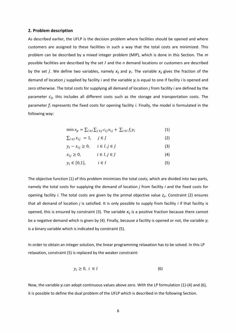
2. Problem description

As described earlier, the UFLP is the decision problem where facilities should be opened and where

customers are assigned to these facilities in such a way that the total costs are minimized. This

problem can be described by a mixed integer problem (MIP), which is done in this Section. The m

possible facilities are described by the set and the n demand locations or customers are described

by the set . We define two variables, namely xij and yi. The variable xij gives the fraction of the

demand of location j supplied by facility i and the variable yi is equal to one if facility i is opened and

zero otherwise. The total costs for supplying all demand of location j from facility i are defined by the

parameter cij, this includes all different costs such as the storage and transportation costs. The

parameter fi represents the fixed costs for opening facility i. Finally, the model is formulated in the

following way:

∑ ∑ ∑ (1)

∑ (2)

(3)

(4)

{ } (5)

The objective function (1) of this problem minimizes the total costs, which are divided into two parts,

namely the total costs for supplying the demand of location j from facility i and the fixed costs for

opening facility i. The total costs are given by the primal objective value zp. Constraint (2) ensures

that all demand of location j is satisfied. It is only possible to supply from facility i if that facility is

opened, this is ensured by constraint (3). The variable xij is a positive fraction because there cannot

be a negative demand which is given by (4). Finally, because a facility is opened or not, the variable yi

is a binary variable which is indicated by constraint (5).

In order to obtain an integer solution, the linear programming relaxation has to be solved. In this LP

relaxation, constraint (5) is replaced by the weaker constraint:

(6)

Now, the variable yi can adopt continuous values above zero. With the LP formulation (1)-(4) and (6),

it is possible to define the dual problem of the UFLP which is described in the following Section.

7

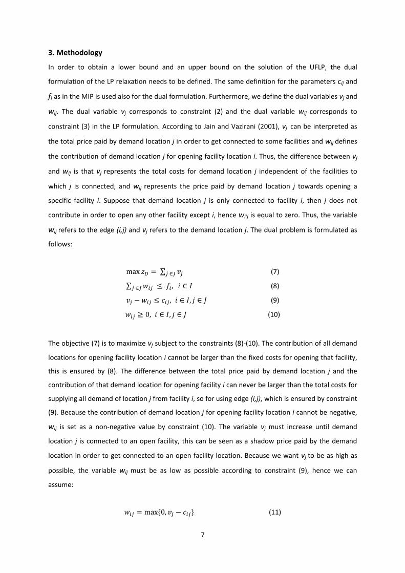
3. Methodology

In order to obtain a lower bound and an upper bound on the solution of the UFLP, the dual

formulation of the LP relaxation needs to be defined. The same definition for the parameters cij and

fi as in the MIP is used also for the dual formulation. Furthermore, we define the dual variables vj and

wij. The dual variable vj corresponds to constraint (2) and the dual variable wij corresponds to

constraint (3) in the LP formulation. According to Jain and Vazirani (2001), vj can be interpreted as

the total price paid by demand location j in order to get connected to some facilities and wij defines

the contribution of demand location j for opening facility location i. Thus, the difference between vj

and wij is that vj represents the total costs for demand location j independent of the facilities to

which j is connected, and wij represents the price paid by demand location j towards opening a

specific facility i. Suppose that demand location j is only connected to facility i, then j does not

contribute in order to open any other facility except i, hence wi’j is equal to zero. Thus, the variable

wij refers to the edge (i,j) and vj refers to the demand location j. The dual problem is formulated as

follows:

∑ (7)

∑ (8)

(9)

(10)

The objective (7) is to maximize vj subject to the constraints (8)-(10). The contribution of all demand

locations for opening facility location i cannot be larger than the fixed costs for opening that facility,

this is ensured by (8). The difference between the total price paid by demand location j and the

contribution of that demand location for opening facility i can never be larger than the total costs for

supplying all demand of location j from facility i, so for using edge (i,j), which is ensured by constraint

(9). Because the contribution of demand location j for opening facility location i cannot be negative,

wij is set as a non-negative value by constraint (10). The variable vj must increase until demand

location j is connected to an open facility, this can be seen as a shadow price paid by the demand

location in order to get connected to an open facility location. Because we want vj to be as high as

possible, the variable wij must be as low as possible according to constraint (9), hence we can

assume:

{ } (11)

8

The proof of (11) is given as follows:

From constraint (9) we know that: this is equal to the inequality .

According to (10) we know that wij must be positive or zero, hence the inequality is

always satisfied when is also positive or zero. When the difference between vj and cij is

negative, then wij must be equal to zero. From this we obtain that wij is equal to the maximum of

zero and . This equality holds because when wij is lower than { }, then it could

be that, if the maximum of zero and is equal to zero, wij takes a negative value which is in

contradiction with (10). And when wij is higher than { }, then there is room to decrease

wij until constraint (9) is not satisfied anymore. In addition, we want that vj is maximized so according

to constraint (9), wij should be as low as possible. These reasons indicate that the value of wij must

be exactly equal to the maximum of zero and .

When (11) is substituted in (8), we get the following simplified dual problem:

∑ (12)

∑ { } (13)

This simplified dual problem is exactly the same problem as the problem described by the

formulation (7)-(10). The objective function (12) remains the same as (7). Then, a substitution of (11)

in (8) results in the constraint (13). Constraints (9) and (10) of the original dual problem are also

represented by constraint (13) through equality (11). This is validated because when (9) is rewritten

into , it is clear that this constraint is always satisfied when wij is defined as the

maximum of zero and , so constraint (9) disappears. Also constraint (10) is always satisfied

when wij is defined as in (11), because the maximum of zero and is always equal to zero or

larger than zero. ZD is the dual objective value which has to be maximized subject to the constraint

(13).

This dual problem can be solved by, besides using a simplex method, a simpler method which uses

the dual ascent procedure and the dual adjustment procedure. With the dual ascent procedure, the

dual solution gives a lower bound on the solution of the UFLP and the corresponding primal integer

solution gives an upper bound on the solution, hence a range is obtained in which the optimal

solution must be located. With the dual adjustment procedure, the solutions obtained by the dual

9

ascent procedure are improved such that a higher, hence better, lower bound and a lower, hence

better, upper bound on the solution are found. Thus, this procedure aims to close the gap between

the primal and dual solutions, this gap is called the duality gap. This dual adjustment procedure is

only used if the dual and primal solutions obtained by the dual ascent procedure violate the

following complementary slackness conditions:

∑ {

} (14)

[

] { } (15)

Where yi* and xij

* are feasible primal solutions and vj* is a feasible dual solution. When the solution

found by the dual ascent procedure violates the complementary slackness conditions, then the

solution is not optimal and we are going to improve the solution using the dual adjustment

procedure. However, if the solution found by the dual ascent procedure satisfies the complementary

slackness conditions, then this solution is an optimal solution and there is no need to search for

another solution. In that case, the dual adjustment procedure is not executed.

3.1 The dual ascent procedure

The dual ascent procedure provides a lower bound and an upper bound on the solution of the UFLP.

This procedure starts with any feasible dual solution , for example when all vj are set equal to zero,

and tries to increase this solution to the next higher value of cij by cycling through the demand

locations j. In this case, cij are the total costs of supplying all demand of location j from facility i, and

vj is an element of the solution . At the beginning of the procedure, we reindex cij in non-decreasing

order for each j as with k=1,…,m. We reindex cij because then all costs are ordered and it is

possible to move through the sequence of costs when we go from k to k+1 for example. As initial

feasible dual solution we use , hence the lowest value of cij for each j. We initialize the subset

of demand locations , which we are going to use in the dual adjustment procedure. In this set of

demand locations, the locations are included for which we want to increase vj. But in this case, we

initialize with the set of all demand locations , hence .

In the first lines of the procedure, we introduce si and k(j). In this algorithm, the variable si checks if

there is some slack on constraint (13), hence if it is possible to increase vj. The variable k(j) is used to

move to the next higher value of the costs

such that we can increase vj with the difference

between these costs and vj. We describe the algorithm for the dual ascent procedure as follows:

10

1.

2. ∑ { }

3. ( ) { }

( ) ( ) ( )

4.

5. While

6. and

7. If

8. { }

9. If ( )

10. If ( )

11. ( )

12.

13. ( ) ( )

14. end

15. For each

16. If

17.

18. end

19. end

20.

21. If

22.

23. end

24. end

25. end

26. end

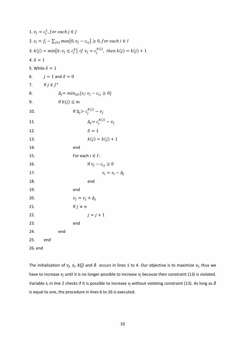
The initialization of vj, si, k(j) and δ occurs in lines 1 to 4. Our objective is to maximize vj, thus we

have to increase vj until it is no longer possible to increase vj because then constraint (13) is violated.

Variable si in line 2 checks if it is possible to increase vj without violating constraint (13). As long as δ

is equal to one, the procedure in lines 6 to 26 is executed.

11

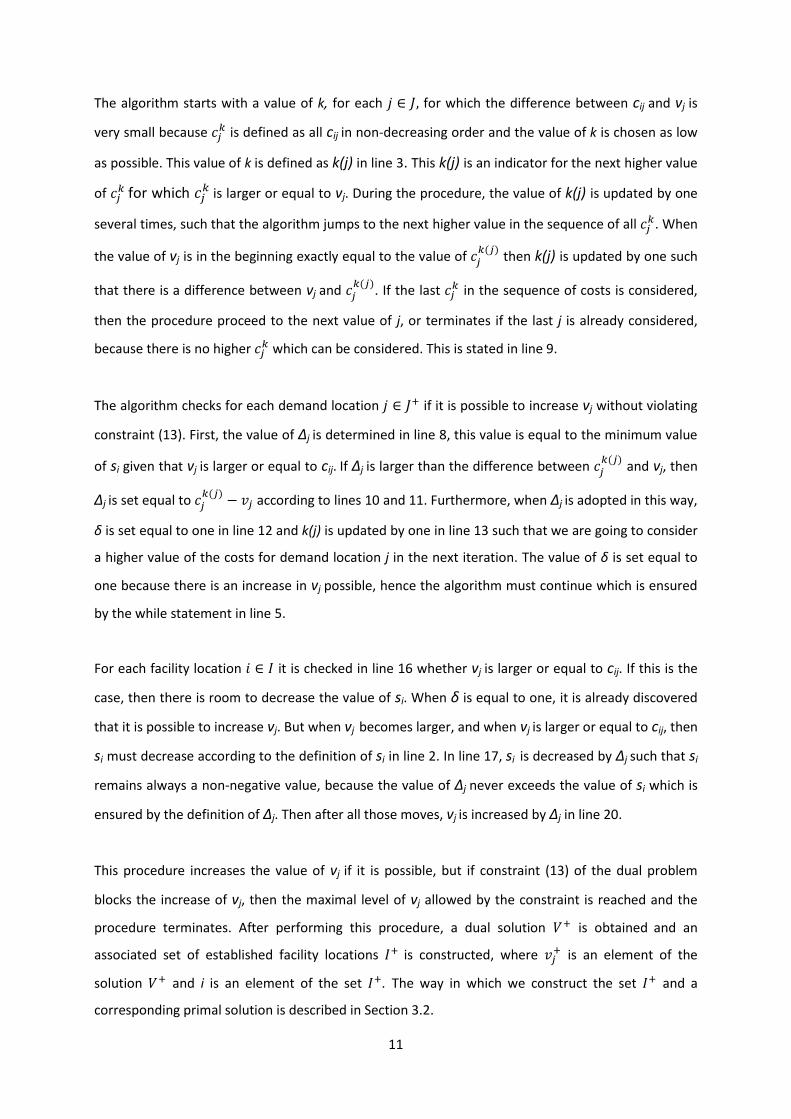
The algorithm starts with a value of k, for each for which the difference between cij and vj is

very small because is defined as all cij in non-decreasing order and the value of k is chosen as low

as possible. This value of k is defined as k(j) in line 3. This k(j) is an indicator for the next higher value

of

for which

is larger or equal to vj. During the procedure, the value of k(j) is updated by one

several times, such that the algorithm jumps to the next higher value in the sequence of all . When

the value of vj is in the beginning exactly equal to the value of ( )

then k(j) is updated by one such

that there is a difference between vj and ( )

. If the last in the sequence of costs is considered,

then the procedure proceed to the next value of j, or terminates if the last j is already considered,

because there is no higher which can be considered. This is stated in line 9.

The algorithm checks for each demand location if it is possible to increase vj without violating

constraint (13). First, the value of Δj is determined in line 8, this value is equal to the minimum value

of si given that vj is larger or equal to cij. If Δj is larger than the difference between ( )

and vj, then

Δj is set equal to ( )

according to lines 10 and 11. Furthermore, when Δj is adopted in this way,

δ is set equal to one in line 12 and k(j) is updated by one in line 13 such that we are going to consider

a higher value of the costs for demand location j in the next iteration. The value of δ is set equal to

one because there is an increase in vj possible, hence the algorithm must continue which is ensured

by the while statement in line 5.

For each facility location it is checked in line 16 whether vj is larger or equal to cij. If this is the

case, then there is room to decrease the value of si. When δ is equal to one, it is already discovered

that it is possible to increase vj. But when vj becomes larger, and when vj is larger or equal to cij, then

si must decrease according to the definition of si in line 2. In line 17, si is decreased by Δj such that si

remains always a non-negative value, because the value of Δj never exceeds the value of si which is

ensured by the definition of Δj. Then after all those moves, vj is increased by Δj in line 20.

This procedure increases the value of vj if it is possible, but if constraint (13) of the dual problem

blocks the increase of vj, then the maximal level of vj allowed by the constraint is reached and the

procedure terminates. After performing this procedure, a dual solution is obtained and an

associated set of established facility locations is constructed, where is an element of the

solution and i is an element of the set . The way in which we construct the set and a

corresponding primal solution is described in Section 3.2.

12

If the solution obtained by the dual ascent procedure violates the complementary slackness

condition (15), then the solution is not optimal and we try to improve the solution using the dual

adjustment procedure. Note that the complementary slackness condition (14) is always satisfied,

which is explained in Section 3.2.

3.2 Opening facilities and obtaining a primal solution

After performing the dual ascent procedure, we obtain the dual solution , which is a sequence of

values of for each demand location j. Furthermore, we obtain for each facility location the slack

variable si. Now we want to know which facilities should be opened. Before we determine this, we

have chosen to set as goal that the complementary slackness conditions (14) and (15) should be

satisfied as much as possible. We have chosen this aim because when the complementary slackness

conditions are satisfied, then we obtain an optimal solution, hence when they are satisfied as much

as possible, we obtain a solution which is as close as possible to the optimal solution.

We have chosen to store the facilities which we might open in the set and the facilities which we

open in reality in the set . By this we mean that in the set , the facilities are included for which

the slack variable si is equal to zero, because then fi is exactly equal to the value of ∑ {

} for each facility i. This indicates that the complementary slackness condition (14) is always

satisfied because ∑ { } is equal to zero for each . This method of

constructing the set is just a choice, there can be several other reasons to store a facility in this set,

such as store all facilities in for which is exactly equal to cij for all demand locations j such that

complementary slackness condition (15) is always satisfied.

The facilities in the set do not all have to be opened, we can make a selection of the facilities that

we could open in order to improve the obtained solution. This set of established facilities is

constructed in the following way. First we are going to check for each facility i from the set how

many demand locations j there are for which is strictly larger than cij. Then we sort the facilities in

descending order on the number of demand locations for which holds. We want to know

this because the complementary slackness condition (15) is satisfied when at most one facility has

, for some j. The reason for this is that the binary variables and

, which correspond to

the used edges and the opened facilities respectively, are both equal to one with certainty for only

the lowest value of cij, hence the difference

is equal to zero in this case, which indicates

that complementary slackness condition (15) is satisfied.

13

This indicates that when there are for some j two or more facilities from for which is strictly

larger than cij, then we have to delete some facilities from the set in order to form the set . For

us it seems the most reasonable choice to delete the facility for which the number of demand

locations for which is the highest, because then for more j, the number of facilities for

which decreases. If for some j there was just one facility for which

, and we delete

that facility, then there are for these demand locations j zero facilities for which holds. If

this is the case, then complementary slackness condition (15) is still satisfied because {

} is equal to zero for these j.

When we have constructed this set , we determine the total costs, hence the opening costs and

transportation costs together, when we open all facilities which are included in . If these total costs

are lower than the total costs determined when all facilities in are opened, we have obtained a

new solution which is better than the solution originally found by the dual ascent procedure. But if

these total costs are not lower than the total costs of the original solution, then we are going to

adapt the set in the following way. We take the set and we delete the facility for which the

number of demand locations for which is the second-highest. Then, we are going to check if

this results in a reduction of total costs. If this is the case, a new solution is found, but if this is not

the case, then the set is adapted again through deleting the facility for which the number of

demand locations for which is the third-highest, and so on until a better solution is found or

all options are considered. If all options of deleting facilities are considered and none of these

options result in a better solution, then the set equals the set Note that in this procedure a

solution is found that is not necessarily the best solution possible. This is because the procedure

stops when a better solution is found than the solution with the set such that for as much as

possible demand locations j, the number of facilities for which decreases, hence the

complementary slackness condition (15) is satisfied as much as possible.

Since we now have a set of opened facilities , we can derive a integer primal solution from this set.

The integer primal solution consists of the variables and

. The variable is a vector of length

m containing all facilities. The facilities which belong to the set , so those which are opened

according to the rule described before, are indicated with one and the closed facilities are indicated

with zero. Furthermore, the variable indicates which demand locations are connected with a

certain facility, hence if the edge (i,j) is used or not. But we do not yet know which demand locations

are connected to facility i. To determine this, we have to make a choice or a rule which we are going

to apply. For us, because we want to minimize costs, it seems obvious that for each demand location

14

j, we search for an established facility i from the set which is the cheapest in supplying the

demand of location j. In this way, we choose for each demand location the facility with the lowest

costs cij, hence the transportation costs that are as low as possible. Another way to formulate this is

that we use the cheapest edge for that demand location. The edges that we want to use are

indicated with one, and the edges that we do not want to use are indicated with zero. If we

summarize this, we can obtain an integer primal solution from a dual solution in the following way:

{

(16)

{

( )

(17)

Where ( ) is a minimum-cost source facility, defined for each demand location j. By this, we

mean that for each demand location j, there is an opened facility i for which the costs of satisfying

the demand of j are the lowest.

Through our definitions of and , the complementary slackness condition (14) is always satisfied

as we have seen earlier. Namely, the facilities in set are facilities for which the difference between

fi and ∑ { } is exactly equal to zero and for these facilities, the value of is equal to

one. Thus, for the established facilities, the complementary slackness condition (14) is always

satisfied. For a closed facility, the value of is equal to zero, hence for the closed facilities condition

(14) is also satisfied.

Complementary slackness condition (15) is satisfied when at most one facility has for

some j as we have seen earlier. This reasoning does not hold with certainty for all cij except the

lowest one, thus we choose the number of demand locations for which for as low as

possible. It is not guaranteed that complementary slackness condition (15) is always satisfied

because it is hardly possible to find a feasible solution where there is at most one facility for

which holds for each j, but through our definition of we try to get as close as possible to

such a feasible solution.

3.3 The dual adjustment procedure

The dual adjustment procedure starts with a solution obtained by the dual ascent procedure for

which not all complementary slackness conditions are satisfied. We also start with the set

obtained by the procedure described in Section 3.2. From this solution, there are some j’ selected for

15

which the complementary slackness condition (15) is violated. Only (15) can be violated because

condition (14) is always satisfied as we have seen earlier. We decrease vj’ which creates slack on the

constraints (13) corresponding to the with vj’ > cij’. After the decrease of vj’, other vj, that are

limited by these constraints (13), are tried to be increased using the dual ascent procedure. If it is

possible to increase more than one vj as vj’ is decreased, then the dual objective will be increased by

this change. This process is performed for all j’ and the procedure is repeated as long as the dual

objective improves. This method makes use of the dual ascent procedure in case where vj is

attempted to be increased.

We define the following sets which are used in the dual adjustment procedure: { }

and { } for each demand location The set

consists of all facilities in the

set for which holds for each . This set is used to create the set , which we will

discuss later. Then we have defined the set , which is in fact a subset of

. In the set , for each

demand location , we store the established facilities from the set for which vj is strictly larger

than cij. This set is used to determine if the solution is already optimal or if it is possible to improve

the current solution, which we will discuss later.

Furthermore, for each we define the set {

{ }} In this set, for each facility i, the

demand locations are given for which the value of is equal to facility i which satisfies .

Hence, this set gives for each facility the demand locations that can be served by this facility and for

which holds. In fact, according to the definition of we do not consider each facility i in this

case, but each i in the set , hence each facility for which the slack variable is equal to zero. This set

is used to check which vj we can increase.

For each with | | , we define a second-best source ( ) whereby the following

property holds with regard to the costs: ( ) ( ) . The second-best source ( ) for

a demand location j is not the cheapest possible facility to supply the demand of j from, namely the

minimum-cost source ( ), but it is the cheapest one when the minimum-cost source is not taken

into account. The second-best source is only defined for a facility i with | | , because when the

number of elements in is smaller or equal to one, then there is simply no second-best source

because there is just one facility that can be opened which forms automatically the minimum-cost

source. For each we define { } The algorithm for the dual adjustment

procedure is described as follows:

16

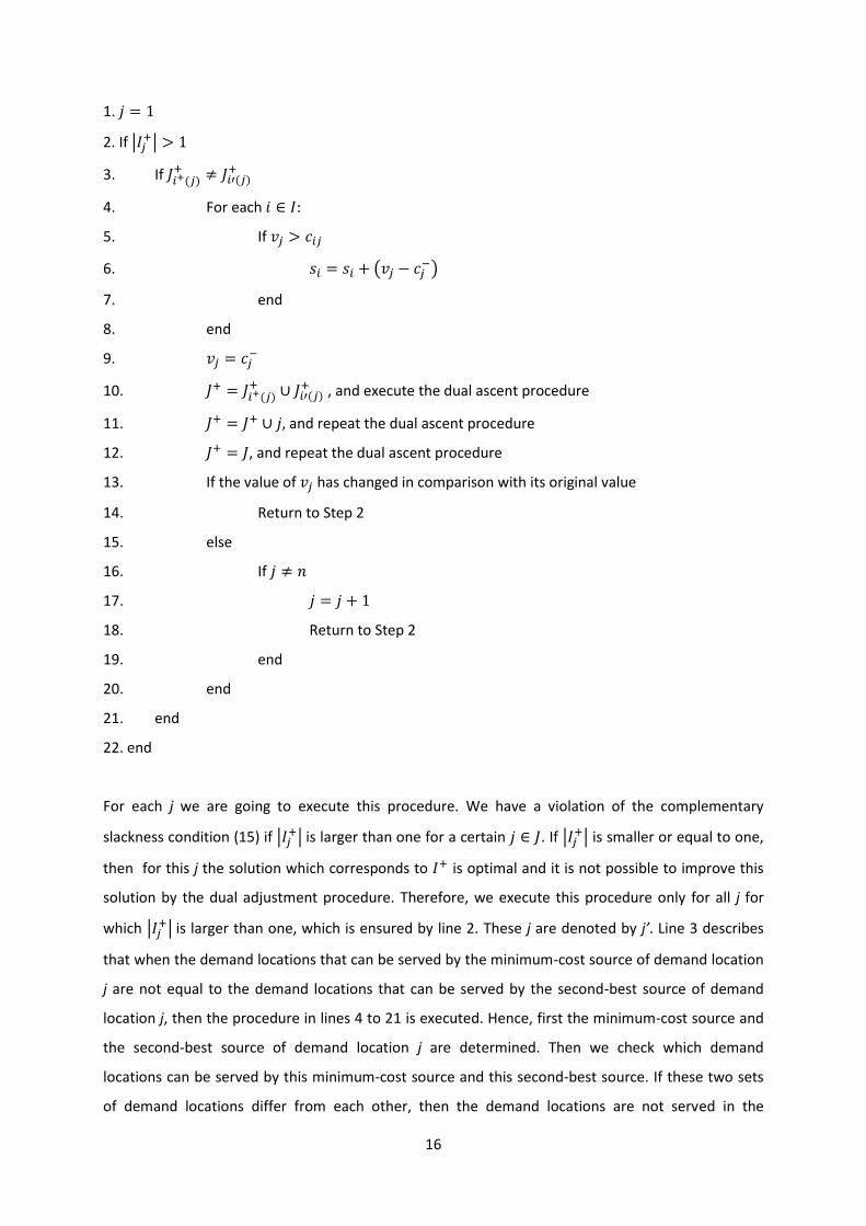
1.

2. If | |

3. If ( ) ( )

4. For each

5. If

6. ( )

7. end

8. end

9.

10. ( ) ( )

, and execute the dual ascent procedure

11. and repeat the dual ascent procedure

12. , and repeat the dual ascent procedure

13. If the value of has changed in comparison with its original value

14. Return to Step 2

15. else

16. If

17.

18. Return to Step 2

19. end

20. end

21. end

22. end

For each j we are going to execute this procedure. We have a violation of the complementary

slackness condition (15) if | | is larger than one for a certain . If |

| is smaller or equal to one,

then for this j the solution which corresponds to is optimal and it is not possible to improve this

solution by the dual adjustment procedure. Therefore, we execute this procedure only for all j for

which | | is larger than one, which is ensured by line 2. These j are denoted by j’. Line 3 describes

that when the demand locations that can be served by the minimum-cost source of demand location

j are not equal to the demand locations that can be served by the second-best source of demand

location j, then the procedure in lines 4 to 21 is executed. Hence, first the minimum-cost source and

the second-best source of demand location j are determined. Then we check which demand

locations can be served by this minimum-cost source and this second-best source. If these two sets

of demand locations differ from each other, then the demand locations are not served in the

17

cheapest possible way, hence by executing lines 4 to 21, an improvement can be found, otherwise

we proceed to the next j’.

In lines 4 to 8, we are going to look if si can be increased for some i. If vj’ is larger than cij’, then for

that i, the complementary slackness condition (15) is violated such that there is slack created on

constraint (13) when vj’ is decreased. This makes it possible that the dual objective can be increased

when two or more other vj that are limited by these constraints (13) are increased. When vj’ is

decreased, then it must be possible to increase si according to the definition of si in line 2 of the dual

ascent procedure. After the increasing of si in lines 4 to 8, we decrease the vj’ for which the

complementary slackness condition (15) is violated, to the value of in line 9.

After the decrease of vj’, we increase other vj that are limited by constraint (13). This is done in lines

10 to 12 by executing the dual ascent procedure. First, the dual ascent procedure is executed when

is equal to ( ) and ( )

together. This means that only for these j, we are going to increase vj if

that is possible. Then we add j to and we repeat the dual ascent procedure in line 11. In order to

obtain a valid solution when the procedure is terminated, we repeat the dual ascent procedure when

is set equal to in line 12. If, after executing the dual ascent procedure three times, the value of vj

is equal to the original value of vj, then vj cannot be improved further and j is increased by one if

possible and we return to Step 2, given in lines 16 to 19. Otherwise, we return to Step 2 without

updating j which is stated by line 14. If all values of j are considered, then the procedure terminates

and a solution is found.

The dual ascent procedure and the dual adjustment procedure result in a solution for the UFLP. This

solution is always feasible because the constraints are always satisfied, which is ensured during the

performance of these methods. The question is, if these methods result in an optimal solution for the

UFLP. In order to obtain an optimal solution, all complementary slackness conditions should be

satisfied. According to our definition of , complementary slackness condition (14) is always

satisfied, as we have described earlier. However, we cannot guarantee that condition (15) is also

always satisfied. This is due to the fact that it is hardly possible to find a feasible solution where for

each it holds that at most one facility from the set has , which is already concluded in

Section 3.2, but it is not impossible that condition (15) is always satisfied. From this reasoning we can

conclude that the dual ascent procedure and the dual adjustment procedure do not always result in

an optimal solution for the UFLP. In order to obtain an optimal solution, a branch-and-bound phase

can be used with the lower and upper bound given by the solutions obtained by these procedures.

18

4. Results

The dual ascent procedure is executed for the three standard problem instances, namely the Bilde-

Krarup, the Galvão Raggi and the Gap B instances. The way in which the dual ascent procedure is

executed is described in Section 3.1. For each problem instance we check if all complementary

slackness conditions are satisfied by the solutions obtained with the dual ascent procedure. If this is

not the case, then the dual adjustment procedure described in Section 3.3 is executed, otherwise an

optimal solution to the LP relaxation of the UFLP is found. In this Section, the results are analysed for

each standard problem instance.

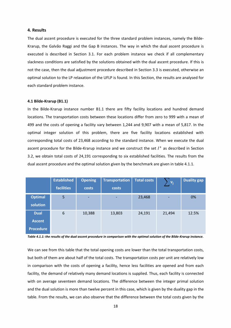
4.1 Bilde-Krarup (B1.1)

In the Bilde-Krarup instance number B1.1 there are fifty facility locations and hundred demand

locations. The transportation costs between these locations differ from zero to 999 with a mean of

499 and the costs of opening a facility vary between 1,244 and 9,907 with a mean of 5,817. In the

optimal integer solution of this problem, there are five facility locations established with

corresponding total costs of 23,468 according to the standard instance. When we execute the dual

ascent procedure for the Bilde-Krarup instance and we construct the set as described in Section

3.2, we obtain total costs of 24,191 corresponding to six established facilities. The results from the

dual ascent procedure and the optimal solution given by the benchmark are given in table 4.1.1.

Established

facilities

Opening

costs

Transportation

costs

Total costs ∑ Duality gap

Optimal

solution

5 - - 23,468 - 0%

Dual

Ascent

Procedure

6 10,388 13,803 24,191 21,494 12.5%

Table 4.1.1: the results of the dual ascent procedure in comparison with the optimal solution of the Bilde-Krarup instance.

We can see from this table that the total opening costs are lower than the total transportation costs,

but both of them are about half of the total costs. The transportation costs per unit are relatively low

in comparison with the costs of opening a facility, hence less facilities are opened and from each

facility, the demand of relatively many demand locations is supplied. Thus, each facility is connected

with on average seventeen demand locations. The difference between the integer primal solution

and the dual solution is more than twelve percent in this case, which is given by the duality gap in the

table. From the results, we can also observe that the difference between the total costs given by the

19

benchmark and the total costs obtained by the dual ascent procedure is relatively small, so we can

conclude that we are close to the optimal solution.

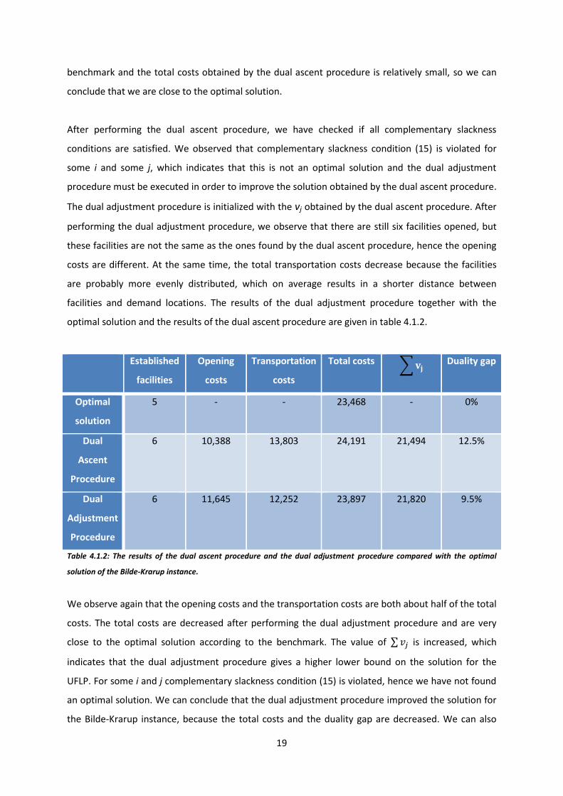
After performing the dual ascent procedure, we have checked if all complementary slackness

conditions are satisfied. We observed that complementary slackness condition (15) is violated for

some i and some j, which indicates that this is not an optimal solution and the dual adjustment

procedure must be executed in order to improve the solution obtained by the dual ascent procedure.

The dual adjustment procedure is initialized with the vj obtained by the dual ascent procedure. After

performing the dual adjustment procedure, we observe that there are still six facilities opened, but

these facilities are not the same as the ones found by the dual ascent procedure, hence the opening

costs are different. At the same time, the total transportation costs decrease because the facilities

are probably more evenly distributed, which on average results in a shorter distance between

facilities and demand locations. The results of the dual adjustment procedure together with the

optimal solution and the results of the dual ascent procedure are given in table 4.1.2.

Established

facilities

Opening

costs

Transportation

costs

Total costs ∑ Duality gap

Optimal

solution

5 - - 23,468 - 0%

Dual

Ascent

Procedure

6 10,388 13,803 24,191 21,494 12.5%

Dual

Adjustment

Procedure

6 11,645 12,252 23,897 21,820 9.5%

Table 4.1.2: The results of the dual ascent procedure and the dual adjustment procedure compared with the optimal

solution of the Bilde-Krarup instance.

We observe again that the opening costs and the transportation costs are both about half of the total

costs. The total costs are decreased after performing the dual adjustment procedure and are very

close to the optimal solution according to the benchmark. The value of ∑ is increased, which

indicates that the dual adjustment procedure gives a higher lower bound on the solution for the

UFLP. For some i and j complementary slackness condition (15) is violated, hence we have not found

an optimal solution. We can conclude that the dual adjustment procedure improved the solution for

the Bilde-Krarup instance, because the total costs and the duality gap are decreased. We can also

20

conclude that the solution obtained by this procedure is close to the optimal solution given by the

benchmark.

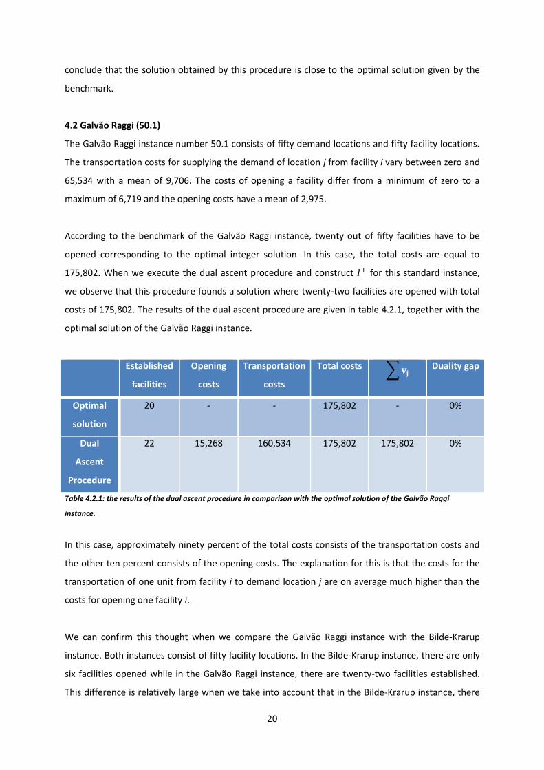
4.2 Galvão Raggi (50.1)

The Galvão Raggi instance number 50.1 consists of fifty demand locations and fifty facility locations.

The transportation costs for supplying the demand of location j from facility i vary between zero and

65,534 with a mean of 9,706. The costs of opening a facility differ from a minimum of zero to a

maximum of 6,719 and the opening costs have a mean of 2,975.

According to the benchmark of the Galvão Raggi instance, twenty out of fifty facilities have to be

opened corresponding to the optimal integer solution. In this case, the total costs are equal to

175,802. When we execute the dual ascent procedure and construct for this standard instance,

we observe that this procedure founds a solution where twenty-two facilities are opened with total

costs of 175,802. The results of the dual ascent procedure are given in table 4.2.1, together with the

optimal solution of the Galvão Raggi instance.

Established

facilities

Opening

costs

Transportation

costs

Total costs ∑ Duality gap

Optimal

solution

20 - - 175,802 - 0%

Dual

Ascent

Procedure

22 15,268 160,534 175,802 175,802 0%

Table 4.2.1: the results of the dual ascent procedure in comparison with the optimal solution of the Galvão Raggi

instance.

In this case, approximately ninety percent of the total costs consists of the transportation costs and

the other ten percent consists of the opening costs. The explanation for this is that the costs for the

transportation of one unit from facility i to demand location j are on average much higher than the

costs for opening one facility i.

We can confirm this thought when we compare the Galvão Raggi instance with the Bilde-Krarup

instance. Both instances consist of fifty facility locations. In the Bilde-Krarup instance, there are only

six facilities opened while in the Galvão Raggi instance, there are twenty-two facilities established.

This difference is relatively large when we take into account that in the Bilde-Krarup instance, there

21

are twice as many demand locations as in the Galvão Raggi instance. This large difference is due to

the fact that in the Bilde-Krarup instance, the opening costs are relatively high in comparison with

the transportation costs, and in the Galvão Raggi instance this relationship is reversed.

For the solution obtained by the dual ascent procedure, all complementary slackness conditions are

satisfied, hence the optimal solution is found by the dual ascent procedure and we do not execute

the dual adjustment procedure. This can also be confirmed by the fact that the total costs found by

the dual ascent procedure are exactly the same as the total costs given by the benchmark, hence the

duality gap is equal to zero percent and the solution cannot be improved.

4.3 Gap B (1031)

Number 1031 of the Gap B instance consists of hundred possible facility locations and hundred

demand locations. The costs of transportation between facilities and demand locations are in most

cases equal to 48,029, which is the maximum of the transportation costs, and in some cases the

transportation costs are very low, for example one or two. For this reason, the mean of the

transportation costs is relatively high, namely 43,226. Furthermore, the costs of opening a facility are

for each facility equal to 3,000.

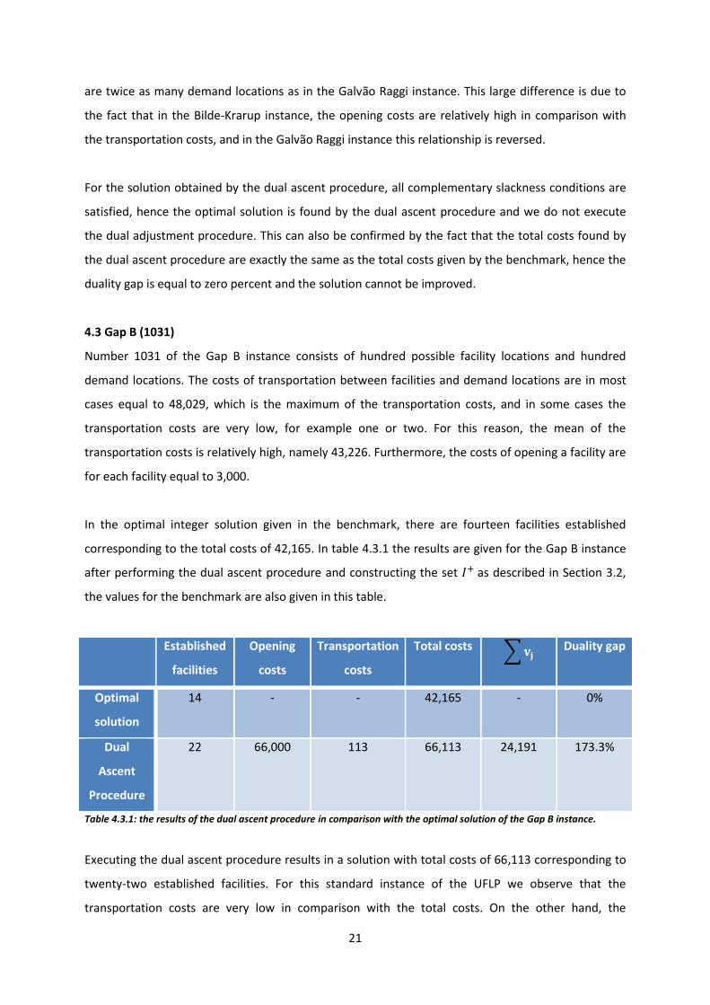
In the optimal integer solution given in the benchmark, there are fourteen facilities established

corresponding to the total costs of 42,165. In table 4.3.1 the results are given for the Gap B instance

after performing the dual ascent procedure and constructing the set as described in Section 3.2,

the values for the benchmark are also given in this table.

Established

facilities

Opening

costs

Transportation

costs

Total costs ∑ Duality gap

Optimal

solution

14 - - 42,165 - 0%

Dual

Ascent

Procedure

22 66,000 113 66,113 24,191 173.3%

Table 4.3.1: the results of the dual ascent procedure in comparison with the optimal solution of the Gap B instance.

Executing the dual ascent procedure results in a solution with total costs of 66,113 corresponding to

twenty-two established facilities. For this standard instance of the UFLP we observe that the

transportation costs are very low in comparison with the total costs. On the other hand, the

22

contribution of the opening costs to the total costs is very high. The explanation for this is that the

opening costs are the same for each facility, hence for each demand location, the facility with the

lowest transportation costs is established. For some facilities, the transportation costs to certain

demand locations are between zero and five, hence these facilities are established to supply the

demand of the demand locations with the lowest transportation costs.

The difference between the total costs corresponding to the optimal solution given in the benchmark

and the total costs observed by the dual ascent procedure is relatively large, namely more than

twenty thousand. This difference is explained by the fact that in the optimal solution, there are

fourteen facilities opened while in the solution obtained by the dual ascent procedure, there are

twenty-two facilities established, so eight facilities more. These eight extra facilities provide

additional opening costs of twenty-four thousand, which is approximately the difference in total

costs between the two cases. Furthermore, we obtain that the duality gap is very large, namely more

than hundred seventy percent. This large difference between the primal integer solution and the

dual solution also indicates that we are not close to the optimal solution.

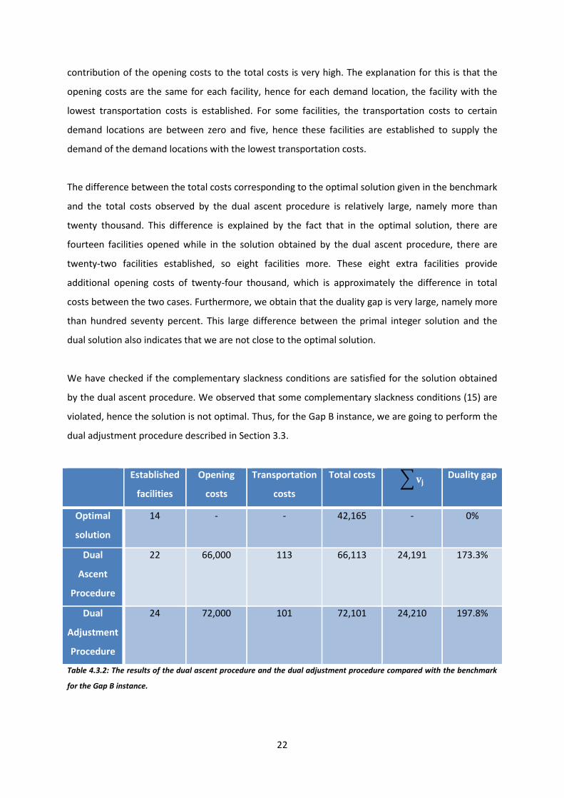
We have checked if the complementary slackness conditions are satisfied for the solution obtained

by the dual ascent procedure. We observed that some complementary slackness conditions (15) are

violated, hence the solution is not optimal. Thus, for the Gap B instance, we are going to perform the

dual adjustment procedure described in Section 3.3.

Established

facilities

Opening

costs

Transportation

costs

Total costs ∑ Duality gap

Optimal

solution

14 - - 42,165 - 0%

Dual

Ascent

Procedure

22 66,000 113 66,113 24,191 173.3%

Dual

Adjustment

Procedure

24 72,000 101 72,101 24,210 197.8%

Table 4.3.2: The results of the dual ascent procedure and the dual adjustment procedure compared with the benchmark

for the Gap B instance.

23

The results of the dual adjustment procedure for the Gap B instance are given in table 4.3.2, together

with the optimal solution and the results of the dual ascent procedure. The value of ∑ is increased

when the dual adjustment procedure is performed, which is expected because the dual adjustment

procedure gives an improvement for the lower bound, hence a higher lower bound, on the solution

for the UFLP. Furthermore, the total costs are increased because there are more facilities

established, namely twenty-four instead of twenty-two. Because of this increasing number of

established facilities, the transportation costs are decreased a bit. The increase of total costs is not

expected because when the value of ∑ increases, the total costs must decrease in order to obtain

a better, hence lower, upper bound.

We observe that the duality gap has increased to almost two hundred percent after performing the

dual adjustment procedure, this indicates that we have obtained a solution which is far from the

optimal solution. The dual adjustment procedure results in total costs of 72,101 which also indicates

that this solution is not close to the optimal solution given by the benchmark and which is not an

improvement of the solution found by the dual ascent procedure. From this reasoning we can

conclude that the dual ascent procedure and especially the dual adjustment procedure perform not

very well for the Gap B instance.

4.3.1 Changes in transportation costs

We want to explain this bad performance of the dual ascent procedure and the dual adjustment

procedure for the Gap B instance. It seems as if the algorithm is focused on keeping the total

transportation costs as low as possible, but then the number of facilities rises as we can see in table

4.3.2. In order to check the impact of the relatively low transportation costs on the performance of

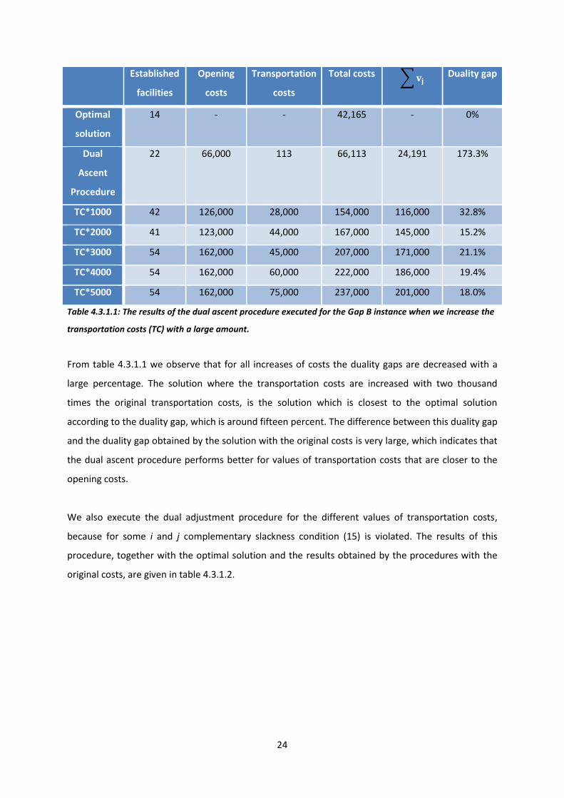
the two procedures, we increase the transportation costs with a large amount, and we execute the

dual ascent procedure. The results are shown in table 4.3.1.1, where we assume that the opening

costs remain the same in each case.

We have executed the dual ascent procedure when we increase the transportation costs with one

thousand, two thousand, three thousand, four thousand and five thousand times the original

transportation costs. We have chosen this scale because then, the transportation costs of the

cheapest edges, which are generally used and are in most of the cases equal to one, are close to the

opening costs of three thousand when we multiply the original costs with three thousand. And

because we want to analyse what happens to the solution if the transportation costs are a bit lower

and a bit higher than the opening costs, we have also multiplied the transportation costs by one

thousand, two thousand, four thousand and five thousand.

24

Established

facilities

Opening

costs

Transportation

costs

Total costs ∑ Duality gap

Optimal

solution

14 - - 42,165 - 0%

Dual

Ascent

Procedure

22 66,000 113 66,113 24,191 173.3%

TC*1000 42 126,000 28,000 154,000 116,000 32.8%

TC*2000 41 123,000 44,000 167,000 145,000 15.2%

TC*3000 54 162,000 45,000 207,000 171,000 21.1%

TC*4000 54 162,000 60,000 222,000 186,000 19.4%

TC*5000 54 162,000 75,000 237,000 201,000 18.0%

Table 4.3.1.1: The results of the dual ascent procedure executed for the Gap B instance when we increase the

transportation costs (TC) with a large amount.

From table 4.3.1.1 we observe that for all increases of costs the duality gaps are decreased with a

large percentage. The solution where the transportation costs are increased with two thousand

times the original transportation costs, is the solution which is closest to the optimal solution

according to the duality gap, which is around fifteen percent. The difference between this duality gap

and the duality gap obtained by the solution with the original costs is very large, which indicates that

the dual ascent procedure performs better for values of transportation costs that are closer to the

opening costs.

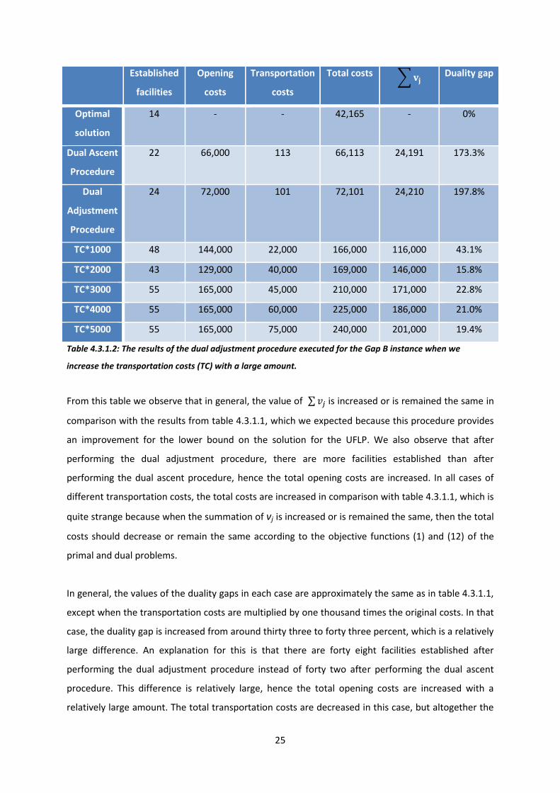
We also execute the dual adjustment procedure for the different values of transportation costs,

because for some i and j complementary slackness condition (15) is violated. The results of this

procedure, together with the optimal solution and the results obtained by the procedures with the

original costs, are given in table 4.3.1.2.

25

Established

facilities

Opening

costs

Transportation

costs

Total costs ∑ Duality gap

Optimal

solution

14 - - 42,165 - 0%

Dual Ascent

Procedure

22 66,000 113 66,113 24,191 173.3%

Dual

Adjustment

Procedure

24 72,000 101 72,101 24,210 197.8%

TC*1000 48 144,000 22,000 166,000 116,000 43.1%

TC*2000 43 129,000 40,000 169,000 146,000 15.8%

TC*3000 55 165,000 45,000 210,000 171,000 22.8%

TC*4000 55 165,000 60,000 225,000 186,000 21.0%

TC*5000 55 165,000 75,000 240,000 201,000 19.4%

Table 4.3.1.2: The results of the dual adjustment procedure executed for the Gap B instance when we

increase the transportation costs (TC) with a large amount.

From this table we observe that in general, the value of ∑ is increased or is remained the same in

comparison with the results from table 4.3.1.1, which we expected because this procedure provides

an improvement for the lower bound on the solution for the UFLP. We also observe that after

performing the dual adjustment procedure, there are more facilities established than after

performing the dual ascent procedure, hence the total opening costs are increased. In all cases of

different transportation costs, the total costs are increased in comparison with table 4.3.1.1, which is

quite strange because when the summation of vj is increased or is remained the same, then the total

costs should decrease or remain the same according to the objective functions (1) and (12) of the

primal and dual problems.

In general, the values of the duality gaps in each case are approximately the same as in table 4.3.1.1,

except when the transportation costs are multiplied by one thousand times the original costs. In that

case, the duality gap is increased from around thirty three to forty three percent, which is a relatively

large difference. An explanation for this is that there are forty eight facilities established after

performing the dual adjustment procedure instead of forty two after performing the dual ascent

procedure. This difference is relatively large, hence the total opening costs are increased with a

relatively large amount. The total transportation costs are decreased in this case, but altogether the

26

total costs are increased with twelve thousand while the value of ∑ is not changed, this indicates

why the duality gap is increased with such a large difference.

We can conclude that the dual ascent procedure performs better for the Gap B instance when the

difference between the transportation costs and the opening costs is smaller. But we can also

conclude that the dual adjustment procedure performs not very well because the total costs increase

and the duality gap increases, hence this procedure does not provide an improvement of the solution

found by the dual ascent procedure, which it should actually do. When we compare this with the

results in Section 4.3, we obtain the same pattern, namely that the dual adjustment procedure does

not provide an improvement on the solution found by the dual ascent procedure. From this, we

could conclude that the bad performance of both procedures together is particularly due to the bad

performance of the dual adjustment procedure.

Now, we want to know what is the cause of the bad performance of the dual adjustment procedure

in the case in which there is a large difference between the opening costs for one facility and the

transportation costs for one edge, and when there is a large difference between transportation costs

themselves, so in case of the Gap B instance. We have to look into the steps of the procedure for

something that is not going well.

From the dual ascent procedure, we obtain values of vj that are very low, between zero and seven, or

very high, namely around three thousand. Because most of the transportation costs are equal to

48,029, there are very few vj that are strictly larger than cij. Hence, when we look at the definition of

, we observe that the values of cij for which holds are always between zero and five. This

indicates that the value of is also always between zero and five. In line 9 of the dual adjustment

procedure, vj is decreased to , hence to a value between zero and five. Because of this step in the

procedure, it might be that the value of ∑ does not increase so much, hence the dual objective

value will not improve much in this case such that the dual adjustment procedure does not provide

an improvement for the solution found by the dual ascent procedure. For us, through the definition

of it seems most likely that the dual adjustment procedure cannot handle large differences

between transportation costs themselves very well.

27

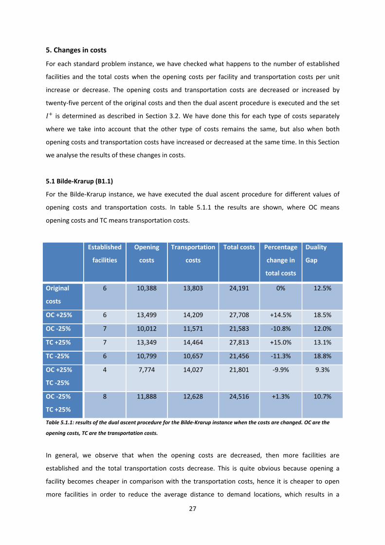
5. Changes in costs

For each standard problem instance, we have checked what happens to the number of established

facilities and the total costs when the opening costs per facility and transportation costs per unit

increase or decrease. The opening costs and transportation costs are decreased or increased by

twenty-five percent of the original costs and then the dual ascent procedure is executed and the set

is determined as described in Section 3.2. We have done this for each type of costs separately

where we take into account that the other type of costs remains the same, but also when both

opening costs and transportation costs have increased or decreased at the same time. In this Section

we analyse the results of these changes in costs.

5.1 Bilde-Krarup (B1.1)

For the Bilde-Krarup instance, we have executed the dual ascent procedure for different values of

opening costs and transportation costs. In table 5.1.1 the results are shown, where OC means

opening costs and TC means transportation costs.

Established

facilities

Opening

costs

Transportation

costs

Total costs Percentage

change in

total costs

Duality

Gap

Original

costs

6 10,388 13,803 24,191 0% 12.5%

OC +25% 6 13,499 14,209 27,708 +14.5% 18.5%

OC -25% 7 10,012 11,571 21,583 -10.8% 12.0%

TC +25% 7 13,349 14,464 27,813 +15.0% 13.1%

TC -25% 6 10,799 10,657 21,456 -11.3% 18.8%

OC +25%

TC -25%

4 7,774 14,027 21,801 -9.9% 9.3%

OC -25%

TC +25%

8 11,888 12,628 24,516 +1.3% 10.7%

Table 5.1.1: results of the dual ascent procedure for the Bilde-Krarup instance when the costs are changed. OC are the

opening costs, TC are the transportation costs.

In general, we observe that when the opening costs are decreased, then more facilities are

established and the total transportation costs decrease. This is quite obvious because opening a

facility becomes cheaper in comparison with the transportation costs, hence it is cheaper to open

more facilities in order to reduce the average distance to demand locations, which results in a

28

reduction of total transportation costs. If the opening costs are increased, then it becomes more

expensive to open a facility, hence less or the same number of facilities are established.

When the transportation costs are increased, then there are in general more facilities opened, such

that the distance between facilities and the demand locations becomes smaller. Because of this

reason, the total opening costs increase while the total transportation costs do not differ very much

from the original total transportation costs.

From this table, we observe that an increase in the transportation costs of twenty-five percent

results in the largest relative increase in total costs, namely an increase of fifteen percent.

Furthermore, a decrease of twenty-five percent in the transportation costs results in the largest

relative reduction in total costs, namely a reduction of more than eleven percent. Both observations

imply that changes in transportation costs have the greatest impact on the total costs for this

standard instance. Furthermore, we observe that the duality gap is the smallest when the opening

costs are increased and the transportation costs are decreased with twenty-five percent. This

indicates that the dual ascent procedure results in a solution which is the closest to the optimal

solution when the transportation costs are decreased and the opening costs are increased at the

same time with twenty-five percent.

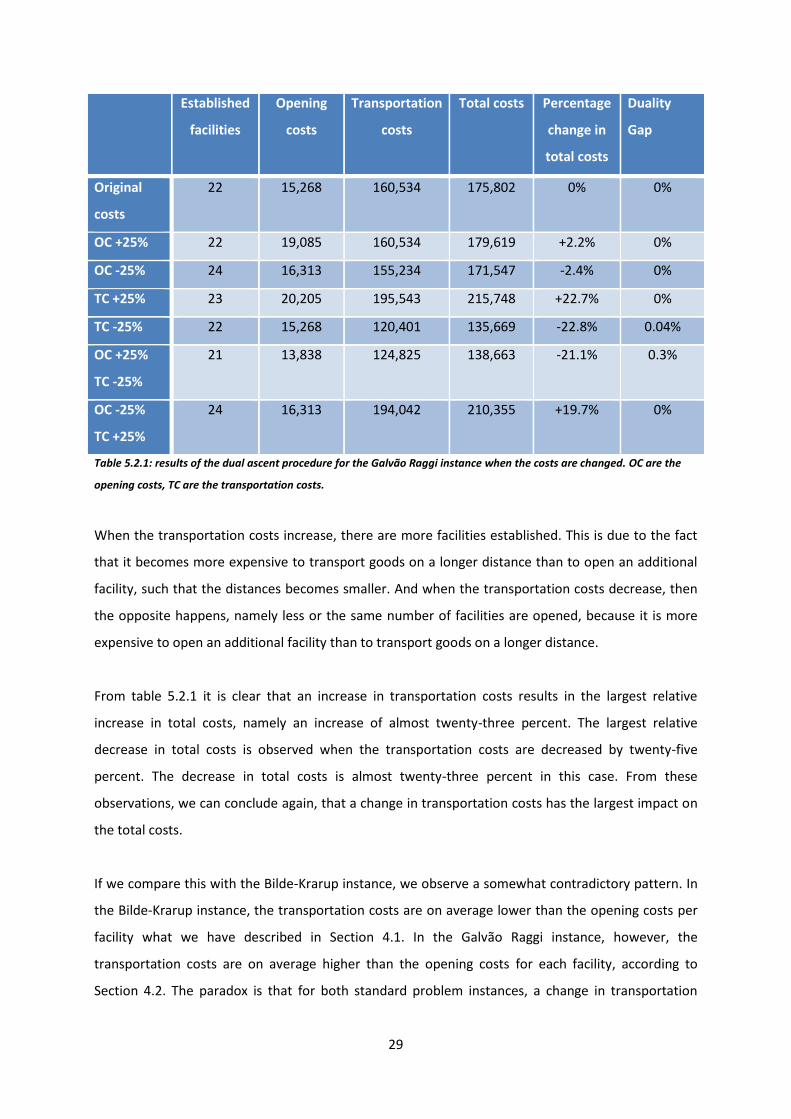
5.2 Galvão Raggi (50.1)

For the Galvão Raggi instance, we have also increased and decreased the opening and transportation

costs in order to observe what happens to the number of established facilities and the total costs.

The dual ascent procedure is executed for the Galvão Raggi instance for the different costs given in

table 5.2.1. The results are also given in this table.

Again, we observe that when the opening costs decrease, then there are more facilities established

because it becomes cheaper to open a facility. When the opening costs increase, then there are less

or the same number of facilities established. This is because it becomes more expensive to open a

facility and it might be more profitable to increase the distance between a facility and a demand

location while opening less facilities.

29

Established

facilities

Opening

costs

Transportation

costs

Total costs Percentage

change in

total costs

Duality

Gap

Original

costs

22 15,268 160,534 175,802 0% 0%

OC +25% 22 19,085 160,534 179,619 +2.2% 0%

OC -25% 24 16,313 155,234 171,547 -2.4% 0%

TC +25% 23 20,205 195,543 215,748 +22.7% 0%

TC -25% 22 15,268 120,401 135,669 -22.8% 0.04%

OC +25%

TC -25%

21 13,838 124,825 138,663 -21.1% 0.3%

OC -25%

TC +25%

24 16,313 194,042 210,355 +19.7% 0%

Table 5.2.1: results of the dual ascent procedure for the Galvão Raggi instance when the costs are changed. OC are the

opening costs, TC are the transportation costs.

When the transportation costs increase, there are more facilities established. This is due to the fact

that it becomes more expensive to transport goods on a longer distance than to open an additional

facility, such that the distances becomes smaller. And when the transportation costs decrease, then

the opposite happens, namely less or the same number of facilities are opened, because it is more

expensive to open an additional facility than to transport goods on a longer distance.

From table 5.2.1 it is clear that an increase in transportation costs results in the largest relative

increase in total costs, namely an increase of almost twenty-three percent. The largest relative

decrease in total costs is observed when the transportation costs are decreased by twenty-five

percent. The decrease in total costs is almost twenty-three percent in this case. From these

observations, we can conclude again, that a change in transportation costs has the largest impact on

the total costs.

If we compare this with the Bilde-Krarup instance, we observe a somewhat contradictory pattern. In

the Bilde-Krarup instance, the transportation costs are on average lower than the opening costs per

facility what we have described in Section 4.1. In the Galvão Raggi instance, however, the

transportation costs are on average higher than the opening costs for each facility, according to

Section 4.2. The paradox is that for both standard problem instances, a change in transportation

30

costs has the greatest impact on the total costs, while for both problem instances the relation

between transportation costs and opening costs is different. A possible explanation for this is that in

the Galvão Raggi instance, ninety percent of the total costs consists of the transportation costs,

hence a change in transportation costs results in a relatively large change in the total costs in this

case.

Another possible explanation for this paradox is the difference in number of demand locations for

each standard instance. In the Bilde-Krarup instance, there are hundred demand locations, so

hundred edges used. In the Galvão Raggi instance, there are fifty demand locations, thus there are

fifty edges used in this case.

Thus, when the transportation costs increase with twenty-five percent, then in the Bilde-Krarup

instance, this has a large effect on the total transportation costs because there are relatively many

edges to which the costs are related, but the opening costs are on average higher than the

transportation costs in this case. When the transportation costs increase with the same percentage

in the Galvão Raggi instance, this has a large effect on the total transportation costs, because the

transportation costs are on average higher than the opening costs and also because the

transportation costs contribute for approximately ninety percent to the total costs for this standard

problem instance.

In addition, in the Galvão Raggi instance, there are on average two demand locations connected with

one facility. Hence, it is hardly possible to decrease the average distance between a facility and a

corresponding demand location further, without increasing the opening costs too much. So, when

the transportation costs increase, the average distance between facilities and demand locations

cannot be reduced so much, hence the total transportation costs increase with almost twenty-two

percent, which is relatively much in comparison with the relative increase of total transportation

costs of fifteen percent in the Bilde-Krarup instance.

The original solution found by the dual ascent procedure for this instance is already an optimal

solution, hence with a duality gap of zero percent. When we change some costs, the dual ascent

procedure still finds solutions that are optimal or very close to an optimal solution, which we can

conclude from the duality gaps. Thus, also when the costs change, the dual ascent procedure

performs well for the Galvão Raggi instance.

31

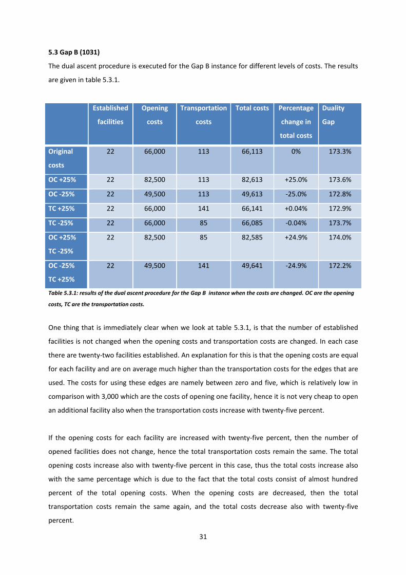
5.3 Gap B (1031)

The dual ascent procedure is executed for the Gap B instance for different levels of costs. The results

are given in table 5.3.1.

Established

facilities

Opening

costs

Transportation

costs

Total costs Percentage

change in

total costs

Duality

Gap

Original

costs

22 66,000 113 66,113 0% 173.3%

OC +25% 22 82,500 113 82,613 +25.0% 173.6%

OC -25% 22 49,500 113 49,613 -25.0% 172.8%

TC +25% 22 66,000 141 66,141 +0.04% 172.9%

TC -25% 22 66,000 85 66,085 -0.04% 173.7%

OC +25%

TC -25%

22 82,500 85 82,585 +24.9% 174.0%

OC -25%

TC +25%

22 49,500 141 49,641 -24.9% 172.2%

Table 5.3.1: results of the dual ascent procedure for the Gap B instance when the costs are changed. OC are the opening

costs, TC are the transportation costs.

One thing that is immediately clear when we look at table 5.3.1, is that the number of established

facilities is not changed when the opening costs and transportation costs are changed. In each case

there are twenty-two facilities established. An explanation for this is that the opening costs are equal

for each facility and are on average much higher than the transportation costs for the edges that are

used. The costs for using these edges are namely between zero and five, which is relatively low in

comparison with 3,000 which are the costs of opening one facility, hence it is not very cheap to open

an additional facility also when the transportation costs increase with twenty-five percent.

If the opening costs for each facility are increased with twenty-five percent, then the number of

opened facilities does not change, hence the total transportation costs remain the same. The total

opening costs increase also with twenty-five percent in this case, thus the total costs increase also

with the same percentage which is due to the fact that the total costs consist of almost hundred

percent of the total opening costs. When the opening costs are decreased, then the total

transportation costs remain the same again, and the total costs decrease also with twenty-five

percent.

32

An increase in transportation costs of twenty-five percent causes an increase in total costs of almost

a half percent. The total opening costs remain the same in this case, but the total transportation

costs rise with twenty-five percent. Because the total transportation costs are less than one percent

of the total costs, the total costs rise with much less than twenty-five percent, namely a half percent.

A decrease in transportation costs with twenty-five percent causes a decrease in total costs of almost

a half percent, this is due to the same reason as described above.

The combination of an increase in opening costs and a decrease in transportation costs of twenty-

five percent causes an increase in total opening costs of twenty-five percent and a decrease in

transportation costs which is almost negligible when we compare it with the total costs, hence the

total costs increase with almost twenty-five percent. When the opening costs are decreased and the

transportation costs are increased with twenty-five percent, the total opening costs decrease also

with twenty-five percent and the total transportation costs increase with almost twenty-five percent

of the original transportation costs. But because the transportation costs are just a very small

percentage of the total costs, the total costs decrease with almost twenty-five percent.

We observed that the opening costs have the greatest impact on the total costs for this problem

instance. The explanation for this observation is that the total costs consist for almost hundred

percent of the opening costs, hence a change in transportation costs matters relatively little for the

change in total costs.

33

6. Another structure of

We think it is possible to improve the solutions of the Bilde-Krarup and the Gap B instance in Section

4 by constructing the set in another way. We construct the set in the same way as before,

namely we include in all facilities for which the slack variable si is equal to zero. From that set, we

construct in the following way. First, we delete the first facility from the set , and the remaining

facilities are stored in the set . Then, we determine the total costs when we open the facilities in

set and we store these total costs. After that, we take the original set and we delete the second

facility. The remaining facilities are stored in the set . Again, we determine the total costs and we

store them. Due to this procedure, it is always the case that in the set , there is one facility less

than in the set

Thus, each time we remove one facility from and we store the remaining facilities in the set We

determine each time the total costs for different sets and when all facilities from the set are

removed once, we choose the set with the lowest total costs. If none of the sets results in

lower total costs, then set is equal to the set The difference with this approach and the

approach in Section 3.2 is that in this approach we do not sort the facilities in descending order on

the number of demand locations for which holds, but we remove all facilities once where

the sequence of removing does not make sense in this case. The approach in Section 3.2 is focused

on satisfying complementary slackness condition (15), while the approach in this Section is focused

on selecting the set for which the total costs are the lowest. We have executed the dual ascent

procedure and the dual adjustment procedure for the Bilde-Krarup and the Gap B instance, because

for these instances we have not yet found an optimal solution in contrast to the Galvão Raggi

instance from which we cannot improve the solution further.

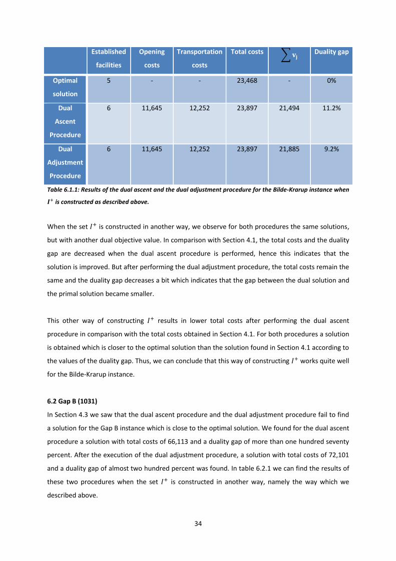
6.1 Bilde-Krarup (B1.1)

In table 6.1.1 the results of the dual ascent procedure and the dual adjustment procedure are given

together with the values of the optimal solution. In order to obtain these results, the set is

constructed as described above. From Section 4.1 we observe a solution with total costs of 24,191

and a duality gap of more than twelve percent after performing the dual ascent procedure. When the

dual adjustment procedure is executed, we observe a solution with total costs of 23,897 and a

duality gap of nine and a half percent.

34

Established

facilities

Opening

costs

Transportation

costs

Total costs ∑ Duality gap

Optimal

solution

5 - - 23,468 - 0%

Dual

Ascent

Procedure

6 11,645 12,252 23,897 21,494 11.2%

Dual

Adjustment

Procedure

6 11,645 12,252 23,897 21,885 9.2%

Table 6.1.1: Results of the dual ascent and the dual adjustment procedure for the Bilde-Krarup instance when

is constructed as described above.

When the set is constructed in another way, we observe for both procedures the same solutions,

but with another dual objective value. In comparison with Section 4.1, the total costs and the duality

gap are decreased when the dual ascent procedure is performed, hence this indicates that the

solution is improved. But after performing the dual adjustment procedure, the total costs remain the

same and the duality gap decreases a bit which indicates that the gap between the dual solution and

the primal solution became smaller.

This other way of constructing results in lower total costs after performing the dual ascent

procedure in comparison with the total costs obtained in Section 4.1. For both procedures a solution

is obtained which is closer to the optimal solution than the solution found in Section 4.1 according to

the values of the duality gap. Thus, we can conclude that this way of constructing works quite well

for the Bilde-Krarup instance.

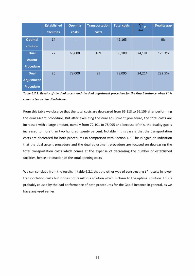
6.2 Gap B (1031)

In Section 4.3 we saw that the dual ascent procedure and the dual adjustment procedure fail to find

a solution for the Gap B instance which is close to the optimal solution. We found for the dual ascent

procedure a solution with total costs of 66,113 and a duality gap of more than one hundred seventy

percent. After the execution of the dual adjustment procedure, a solution with total costs of 72,101

and a duality gap of almost two hundred percent was found. In table 6.2.1 we can find the results of

these two procedures when the set is constructed in another way, namely the way which we

described above.

35

Established

facilities

Opening

costs

Transportation

costs

Total costs ∑ Duality gap

Optimal

solution

14 - - 42,165 - 0%

Dual

Ascent

Procedure

22 66,000 109 66,109 24,191 173.3%

Dual

Adjustment

Procedure

26 78,000 95 78,095 24,214 222.5%

Table 6.2.1: Results of the dual ascent and the dual adjustment procedure for the Gap B instance when is

constructed as described above.

From this table we observe that the total costs are decreased from 66,113 to 66,109 after performing

the dual ascent procedure. But after executing the dual adjustment procedure, the total costs are

increased with a large amount, namely from 72,101 to 78,095 and because of this, the duality gap is

increased to more than two hundred twenty percent. Notable in this case is that the transportation

costs are decreased for both procedures in comparison with Section 4.3. This is again an indication

that the dual ascent procedure and the dual adjustment procedure are focused on decreasing the

total transportation costs which comes at the expense of decreasing the number of established

facilities, hence a reduction of the total opening costs.

We can conclude from the results in table 6.2.1 that the other way of constructing results in lower

transportation costs but it does not result in a solution which is closer to the optimal solution. This is

probably caused by the bad performance of both procedures for the Gap B instance in general, as we

have analysed earlier.

36

7. Conclusion

The Uncapacitated Facility Location Problem consists of m uncapacitated facility locations and n

customers or demand locations. The costs of opening a certain facility i and the costs of supplying all

demand of demand location j from facility i are known and the total of these costs have to be

minimized. In this paper we described that this problem can be formulated as a mixed integer linear

programming problem from which we can derive a linear programming relaxation in order to obtain

an integer solution. We want to find a lower bound and an upper bound on the solution for the UFLP,

hence we have defined a dual formulation of this problem using the LP relaxation. This dual

formulation provides a dual solution for the UFLP where the dual objective value corresponds with a

lower bound and the corresponding primal objective value corresponds with an upper bound for the

solution for the UFLP.

In general, a dual problem can be solved by using a simplex method, but we have performed a

simpler method that contains two methods. The first method we used is called the dual ascent

procedure. This method is based on increasing the initial feasible solution to the next higher value

of the transportation costs by cycling through all demand locations in the set until constraint (13) is

violated. After this procedure, a lower bound and an upper bound on the solution for the UFLP and

the corresponding set of established facilities are obtained. When all complementary slackness

conditions are satisfied, then the solution is optimal. If this is not the case, we try to improve the

obtained solution by executing the dual adjustment procedure.

The dual adjustment procedure starts with the solution obtained by the dual ascent procedure if the

complementary slackness conditions are not satisfied. For some j’ for which the complementary

slackness conditions are not satisfied, we try to decrease vj’ and increase two or more other vj at the

same time such that the dual objective increases. In order to increase vj, the dual ascent procedure,

which is described earlier, is used. This procedure is repeated for all j’ for which the complementary

slackness conditions are violated, as long as the dual objective continues to increase.

We have performed the dual ascent procedure and the dual adjustment procedure for three

standard instances of the UFLP, namely the Bilde-Krarup, the Galvão Raggi and the Gap B instances.

After performing the dual ascent procedure for the Bilde-Krarup instance, we observe that we are

almost close to the optimal solution given by the benchmark. It appeared that not all complementary

slackness conditions are satisfied, hence we executed the dual adjustment procedure. This procedure

provides a solution which is very close to the optimal solution, which indicates that this method

37

based on the dual ascent procedure and the dual adjustment procedure works quite well for the

Bilde-Krarup instance.

After performing the dual ascent procedure for the Galvão Raggi instance, we observe that all

complementary slackness conditions are satisfied, hence an optimal solution is found. The total costs

corresponding with our solution are exactly the same as the total costs given by the benchmark,

namely 175,802, hence the dual ascent procedure works very well for the Galvão Raggi instance and

the dual adjustment procedure do not have to be executed.

For the Gap B instance, the story is a bit different from the other instances. When we perform the

dual ascent procedure for the Gap B instance, some complementary slackness conditions are violated

and the obtained solution is not very close to the optimal solution given by the benchmark. We

found a solution where twenty-two facilities are established with total costs of 66,113 while the

optimal solution given by the benchmark is based on fourteen established facilities with total costs of

42,165. Because there are some complementary slackness conditions violated, we have executed the

dual adjustment procedure in order to improve the solution. The dual adjustment procedure gives a

solution where twenty-four facilities are opened with total costs of 72,101, which is larger than the

total costs found by the dual ascent procedure. We can conclude that the dual ascent procedure and

especially the dual adjustment procedure do not work very well for the Gap B instance. We have

confirmed this thought by increasing the transportation costs with a large amount. After that we

obtain that the dual adjustment procedure provides an improvement of the solution obtained by the

dual ascent procedure. We think that this bad performance of the dual adjustment procedure is

caused by the fact that the value of remains always a low value between zero and five.

For all standard instances, we have checked what would happen if the opening costs and the

transportation costs are increased or decreased. We have increased or decreased one of the two

types of costs with twenty-five percent and we have increased the opening costs with that

percentage while decreasing the transportation costs and vice versa. After executing the dual ascent

procedure for the different values of costs and for the three instances, we observed that changes in

transportation costs have the largest impact on the total costs in the Bilde-Krarup and the Galvão

Raggi instance. For the Gap B instance, changes in opening costs have the largest impact for the total

costs, namely, when the opening costs increase with twenty-five percent, then the total costs also

increase with twenty-five percent. The reason for this is that in the Gap B instance, the total costs

consist for almost hundred percent of the opening costs.

38

We tried another definition of the set in order to improve the solutions found by the dual ascent

procedure and the dual adjustment procedure. This other formulation of results in an

improvement of the solution for the Bilde-Krarup instance. For the Gap B instance it only results in

an improvement of the total transportation costs but not in an improvement of the total costs. This is

also caused by the bad performance of the both procedures for the Gap B instance. From this we can

conclude that another definition of works very well for the Bilde-Krarup instance but not for the

Gap B instance.

From this research we can conclude that the dual ascent procedure and the dual adjustment

procedure work quite well for some of the standard instances, namely the Bilde-Krarup and the

Galvão Raggi instance. The combination of the dual ascent procedure and the dual adjustment

procedure is a fast method to find a feasible solution for these instances. But for the other instance,

namely the Gap B instance, we observed that the combination of the dual ascent procedure and the

dual adjustment procedure has a bad performance in obtaining an optimal solution.

39

8. Discussion and further research

This research is done in a relatively short time period, hence there are some topics that we do not

have considered yet or not completely. In this Section we mention some things in this research that

we could have done differently, and some things for further research.

First, our research is based on the three standard instances of the UFLP. Our choice was to analyse

the Bilde-Krarup, the Galvão Raggi and the Gap B instance, but we could choose several other

standard instances of this problem in order to obtain other results. Next, another choice we made is

the way in which we construct the sets and . In our case, we have defined the set and after

that we have removed one facility each time, according to a specific rule, in order to obtain the set

. But maybe it was better to remove two or three facilities instead of one in order to obtain a

solution with lower total costs. It is just a choice and the construction of and can be done in

several other ways. For further research, it might be interesting to define some other ways in which

we construct and in order to check if it is possible to improve the solutions that we have found

so far.

For the Bilde-Krarup and the Gap B instances, we have not found an optimal solution after executing

the dual ascent procedure and the dual adjustment procedure. As mentioned earlier, when we do

not find an optimal solution using this procedures, we can perform a branch-and-bound procedure

with the bounds given by the solutions that we have found. Because of the time limits, we do not

have executed a branch-and-bound procedure, but this might be an interesting topic for further

research.

We have also looked at what happens to the number of established facilities and the total costs if the

transportation costs or the opening costs change with a certain percentage. We have chosen a

percentage of twenty-five percent because we thought that this would make a significant difference.

It might be interesting for further research to observe what happens with the number of established

facilities and the total costs when the costs are changed with other percentages than twenty-five.

40

References

Dueck, D., Frey, B.J., Jojic, N. and Jojic, V. (2008). Constructing treatment portfolios using

affinity propagation. International conference on research in computational molecular biology.

Erlenkotter, D. (1978). A dual-based procedure for uncapacitated facility location. Operations

Research, Vol. 26, No. 6, pp. 992-1009.

Frank, C. and Romer, K. (2007). Distributed facility location algorithms for flexible

configuration of wireless sensor networks. Distributed computing in sensor systems. Springer.

Jain, K. and Vazirani, V.V. (2001). Primal-dual approximation algorithms for metric facility

location and k-median problems. College of computing, Georgia institute of technology.

Klose, A. and Drexl, A. (2003). Facility location models for distribution system design.

European Journal of Operations Research.

Lazic, N., Frey, B.J. and Aarabi, P. (2010). Solving the uncapacitated facility location problem

using message passing algorithms. Proceedings of the 13th international conference on artificial

intelligence and statistics (AISTATS), Vol. 9, pp. 429-436.

Lazic, N., Givoni, I., Frey, B.J. and Aarabi, P. (2009). Floss: Facility location for subspace

segmentation. International conference on computer vision.

Li, H. (2007). Two-view motion segmentation from linear programming relaxation. Computer

vision and pattern recognition.