91
ANALYSIS OF PARTIAL DIFFERENTIAL EQUATIONS lectures by clément mouhot notes by tony feng

A N A LY S I S O F PA RT I A L D I F F E R E N T I A L E Q U AT I O N S
lectures by clément mouhot
notes by tony feng

A B S T R A C T
These notes are based on lectures given by Clément Mouhot at Cambridge inMichaelmas 2013. However, the original material has been significantly supple-mented by other resources, most notably Evans’s Partial Differential Equations,due to the scribe’s lack of skill. The notes are still rather rough, and all of theerrors should be attributed to the scribe. If you find any, please let me knowabout them at [email protected]
ii

C O N T E N T S
1 introduction 1
1.1 From ODE to PDE 1
1.2 The Cauchy Problem for ODEs 2
1.3 The Cauchy Problem for PDEs 4
2 the cauchy-kovalevskaya theorem 6
2.1 Analytic functions 6
2.2 The Cauchy-Kovalevskaya Theorem for ODEs 8
2.3 The analytic Cauchy problem for PDE. 11
2.4 The Cauchy-Kovalevskaya Theorem for PDE 14
2.5 Counterexamples and Well-Posedness 16
2.6 Classification of PDE 17
3 elliptic equations 21
3.1 Ellipticity 21
3.2 Sobolev Spaces 22
3.3 Elliptic regularity: Dirichlet operator 25
3.4 Hilbert Spaces 28
3.5 Laplace’s equation: Weak Solutions 31
3.6 The Lax-Milgram Theorem and General Elliptic PDE 33
3.7 The Fredholm Alternative 36
3.8 Interior Elliptic Regularity 43
3.9 Boundary elliptic regularity 49
3.10 Maximum Principles 53
3.11 Examples 55
4 hyperbolic equations 58
4.1 Introduction to transport equations 58
4.2 Classical transport equations 59
4.3 Weak solutions 67
4.4 Entropy solutions 73
5 the wave equation 86
5.1 Introduction to the wave equation 86
5.2 Second-order hyperbolic equations 86
5.3 Energy Estimates 87
iii

1I N T R O D U C T I O N
1.1 from ode to pde
The simplest example of a differential equation is the first-order equation
dudx
= F(x)
where F : R→ R is a continuous function. The solution, of course, is given bythe theory of integration:
u(x) = u(x0) +∫ x
x0
F(y) dy.
More generally, an n-th order ordinary differential equation takes the form
F(x, u, u(1), . . . , u(n)) = 0.
In the theory of partial differential equations, we generalize this notion to func-tions of several real variables. We then study solutions to an equation of theform
F(
x0, x1, . . . , xn,∂u∂x0
, . . . ,∂2u
∂xi∂xj, . . . ,
∂3u∂xi∂xj∂xk
)= 0.
There are two (essentially equivalent) viewpoints on how PDE generalize ODE:
1. a PDE is simply an ordinary differential equation in several variables,involving partial derivatives.
2. when one variable can be identified as “time,” the PDE can be interpretedas an ODE trajectory
dudt
= G(u) := G(
x, u,∂u∂xi
,∂2u
∂xi∂xj, . . . ,
∂3u∂xi∂xj∂xk
)in infinite-dimensional functional spaces.
The first viewpoint is more geometrical, while the second brings in infinite-dimensional functional analysis. Either way, it is clear that complex and deepnew phenomena appear, as one is working in a much more subtle geometricspace, or in infinite-dimensional vector spaces where, for instance, there canbe many different norms, and operators are generally unbounded.
Unlike the theory of ODEs, there are not very many general results for PDEs.So we rely instead on guiding principles; in this course, we focus on the fun-damental equations from physics (possibly with careful simplications), empha-sizing the concepts and methods useful to PDEs in general.
1

1.2 the cauchy problem for odes 2
1.2 the cauchy problem for odes
1.2.1 The three main theorems of ODE
Suppose t ∈ I ⊂ R, and we are considering the ODE
u′(t) = F(t, u(t)) (1)
where u : I → Rm. Written out explicitly, this corresponds to the system ofequations
u′1(t) = F1(t, u1, . . . , um)
......
u′m(t) = Fm(t, u1, . . . , um)
plus some initial data. Here F is called the vector field and a solution is called aflow.
There are three main theorems regarding the existence and uniqueness ofsolutions to such a system.
Theorem 1.2.1 (Cauchy-Kovalevskaya). If F is analytic in A ⊂ I ×Rm then thereis a unique local analytic solution to (1) about any point of A.
This is the only result that generalizes in a meaningful way to PDE, and wewill study it in the next chapter.
Theorem 1.2.2 (Picard-Lindelöf/Cauchy-Lipschitz). Suppose F is continuous (inboth variables) and locally Lipschitz in the second argument on A ⊂ I ×Rm. i.e. forany (t0, x0) ∈ A there is an open neighborhood U and a constant C such that for all(t, x) and (t, y) ∈ U, we have
|F(t, x)− F(t, y)| ≤ C|x− y|.
Then there exists a unique local C1-solution to (1).
The idea of the proof is as follows. We want to write the solution as anintegral
u(t) = u(t0) +∫ t
t0
F(s, u(s)) ds.
Of course, this doesn’t make sense, so we turn it into an iterated procedure
u(n+1)(t) = u(t0) +∫ t
t0
F(s, u(n)(s)) ds.
Phrased differently, we can define a function
Φ[u] =(
t 7→ u(t0) +∫ t
t0
F(s, u(s)) ds)
and apply fixed-point theorems to this function in order to show that it con-verges to a solution.
Theorem 1.2.3 (Cauchy-Peano). In the region C ⊂ I ×Rm where F is continuous(in both variables), there exist local C1 solutions.

1.2 the cauchy problem for odes 3
Remark 1.2.4. Note that the theorem does not say anything about uniqueness.It is possible that the solutions bifurcate.
How do you prove this? By using an iterative scheme again, together withthe Arzela-Ascoli compactness theorem.
Example 1.2.5. The differential equationu′(t) =√
u(t)
u(0) = 0
has infinitely many solutions. Indeed, if we solve by the usual method
du√u= dt
then we can integrate to recover a solution provided that u is non-zero. So afamily of solutions is given by u = 1
4 (t− t0)2.
Exercise 1.2.6. Consider the ODEs
u′(t) = 3u(t)2/3
u(0) = 0
and
u′(t) =4u(t)t3
u(t)2 + t4su(0) = 0.
For each, see how many solutions you can find.
1.2.2 Continuation of Solutions: Local vs Global
So far we have discussed local existence and uniqueness of solutions. Whatabout global solutions? If you have global existence and local uniqueness, thenyou can patch together local solutions.
What else could go wrong? The solution could “blow up” in finite time. Thisis a phenomenon that you should keep in mind for the PDE case, where it canbe much more complex.
Example 1.2.7. Consider the ODE
u′(t) = u2
u(0) = u0 > 0.
The solution is u(t) = 1u−1
0 −t, so we have blowup at time T∗ = u−1
0 .
Now consider the ODE
u′(t) = −u2
u(0) = u0 > 0.
This does not blow up; intuitively, the speed decreases the larger u(t) is. Indeeda solution is of the form u(t) = 1
u−10 +t
.

1.3 the cauchy problem for pdes 4
A blow-up requires super-linearity: a function that grows faster than linear at∞. Similarly, a lack of uniqueness is usually related to sublinearity (the vectorfield grows too slowly). However, as we saw above, the sign of the non-linearityplays a crucial role, and this will hold true for PDEs as well.
One way to avoid blowup in finite time is to impose a uniform Lipchitz condi-tion
|F(t, x)| ≤ c(|t||x|).
To prove that this leads to finite solutions, one can establish a bound of theform
|u(t)|2 ≤ eCt|u(0)|2.
One then argues that for any finite time t, u(t) has limit and hence so doesu′(t) (if the vector field is well-behaved). Then one can continue the solutionlocally beyond the point t.
Exercise 1.2.8. (a) Prove that the solution to the pendulum equationu′′(t) + sin u = 0
u(0) = u0 ∈ R
is global. Do the same for the equationu′′(t) + sin(u(t)2) = 0
u(0) = u0 ∈ R
Example 1.2.9. The linear ODE
u′(t) = Au(t)
boils down to a study of the matrix A. If A is diagonalizable, then this is easyto solve component-by-component. Otherwise, use the Jordan form and solvewithin each Jordan block; this is more difficult, but doable.
Example 1.2.10. The contrast of the equations u′(t) =√
u(t) and u′(t) = u(t)2
highlight the principle that sublinearity leads to non-uniqueness and superlin-earity leads to finite time blow-up. We will encounter this again when studyingPDE. The proofs of uniqueness for PDE are much harder due to the presenceof unbounded operators and many different norms.
1.3 the cauchy problem for pdes
A prototypical Cauchy problem in PDE takes the form
∂tu = F(t, x1, . . . , x`, . . . ∂iu, . . . ∂i∂ju, . . .) (2)
u(0, x) = u0(x1, . . . , x`)
where u = u(t, x1, . . . , x`).
Definition 1.3.1. A Cauchy problem of the form (2) is well-posed if
1. there exists a solution,

1.3 the cauchy problem for pdes 5
2. the solution is unique,
3. the solution depends continuously on the boundary data.
The concept of well-posedness was formulated by Hadamard. The importantpoint is that this question depends only the underlying spaces we are consider-ing. In which space to we ask existence, in which space do we ask uniqueness,and for which topology do we ask continuity? There are many possibilities:strong solutions, weak solutions, entropy solutions...Often these are suggestedby the problem itself. On the other hand, we would always like to wind upin a space where the problem is well-posed, which corresponds to “physicallymeaningful” solution.
What happens to the three main results of ODE when we try to extend themto PDE?
1. The Cauchy-Kovalevskaya theorem does extend, in a limited way. It re-quires analyticity of F, and only gives solutions that are local in time.Furthermore, it has some restrictions: F involving only first-order deriva-tives (corresponding to “quasilinear equations”), and must satisfy a “non-characteristic condition.”
Example 1.3.2 (Heat equation). Consider the heat equation ∂u∂t = ∂2u
∂x2
u(0, x) = 11+x2
.
Show that the unique entire series solving this problem has radius ofconvergence in x equal to 0 for any t > 0.
2. The Cauchy-Lipschitz Theorem seems okay, in the sense that the proofgeneralizes quite readily. One needs only fixed-point theorems, whichshould hold broadly in normed vector spaces. However, it turns out thatthe Lipschitz condition almost never holds: one is usually consider dif-ferential operators in infinite-dimensional spaces, which are virtually al-ways unbounded.
3. The Cauchy-Peano Theorem fails to generalize for the same reason thatdifferential operators are generally unbounded and hence discontinuous.However, the basic technique of using discrete approximations and com-pactness arguments does work in PDE settings (with much more work).

2T H E C A U C H Y- K O VA L E V S K AYA T H E O R E M
The Cauchy-Kovalevkaya Theorem is the only one of the three “main theoremsof ODE” that generalizes to PDE, we shall see that it is extremely limited inconsidering only analyticity, and obscures many of the most interesting fea-tures of PDE.
2.1 analytic functions
We begin with some recollections on analytic functions, starting in the one-variable case.
Definition 2.1.1. Let Ω ⊂ R be an open subset. A function f : Ω→ R is analyticat x0 if there exists some open neighborhood U ⊂ Ω containing x0 such thatfor all x ∈ Ω, the Taylor series for f (x) about x0 converges and is equal to f :
f (x) =∞
∑n=0
f (n)(x0)
n!(x− x0)
n.
We say that f is analytic on Ω if it is analytic at all x0 ∈ Ω.
Proposition 2.1.2. Let Ω ⊂ R. A function f : Ω → R is analytic in Ω if and onlyif for every compact subset K ⊂ Ω, there exist constants c(K) and r > 0 such that forall x ∈ K and n ≥ 0, we have
| f (n)(x)| ≤ c(K)n!rn .
Proof. Suppose that f is analytic on Ω and let x0 ∈ Ω. Then in fact f definesa complex analytic function on some open neighborhood of Ω in C. If K ⊂ Ωis a compact subset, then f is holomorphic on an open neighborhood U ⊂ C
containing K. Let M = sup∂U f . Since K is compact, is some δ > 0 separatingany point of K from ∂U. Then by Cauchy’s formula, we have
| f (n)(x)| =∣∣∣∣ (−1)nn!
2πi
∫∂U
f (z)(z− x)n+1 dz
∣∣∣∣ ≤ n!2π
∣∣∣∣2πM
δn+1
∣∣∣∣ .
This is a bound of the desired shape.Conversely, let K be a compact neighborhood of x0 such that | f (n)(x)| ≤
c(K)n!/rn for all x ∈ K. By shrinking r if necessary, we may assume thatK contains B(x0, r/2). We will show that f agrees with its power series onthis open ball. By the theorem on Taylor series with remainder, we have forx ∈ B(x0, r/2)
f (x) =n
∑k=0
f (k)(x0)(x− x0)k
k!+ f (n+1)(x∗)
(x− x0)n+1
(n + 1)!
for some x∗ ∈ B(x0, r/2). By the hypothesis, the remainder term here is∣∣∣∣ f (n+1)(x∗)(x− x0)n+1
(n + 1)!
∣∣∣∣ ≤ c(K)2n+1
6

2.1 analytic functions 7
which convergest to 0 as n→ ∞. Furthermore, hypothesis furnishes a geomet-ric bound on all the summands, so the power series converges in this ball.
Example 2.1.3. Note the distinction between a smooth function, which has aTaylor series, and an analytic function, which has a Taylor series and is equal toit.
• Polynomials, the exponential function, and trigonometric functions arereal analytic. Since analyticity can be detected by the growth of the powerseries coefficients, we see that (finite) sums, products, and compositionsof analytic functions are analytic.
• The function z 7→ z is smooth but not complex-analytic.
• On R, there are smooth functions that are not analytic, such as the bumpfunction
f (x) =
e−1/x2x ≥ 0,
0 x ≤ 0.
We now consider multivariate analytic functions f : Ω → R where Ω ⊂ Rn.Let (x1, . . . , xn) be the coordinates on Ω. For a multi-index α = (α1, . . . , αn) on1, . . . , n we define
xα = xα11 . . . xαn
n and Dα f =∂α1
∂xα11
. . .∂αn
∂xαnn
.
We also set α! = α1! . . . αn!. Then the Taylor series for f about x0 is
f (x) =∞
∑|α|=0
Dα f (x0)
α!(x− x0)
α.
Definition 2.1.4. Let Ω ⊂ Rn be an open subset. A function f : Ω → R isanalytic at x0 if there exists some open neighborhood U ⊂ Ω containing x0
such that for all x ∈ Ω, the Taylor series for f (x) about x0 converges and isequal to f :
f (x) =∞
∑|α|=0
Dα f (x0)
α!(x− x0)
α.
We say that f is analytic on Ω if it is analytic at all x0 ∈ Ω.
As before, analyticity is equivalent to growth control on the derivatives.
Proposition 2.1.5. Let Ω ⊂ Rn. A function f : Ω → R is analytic in Ω if and onlyif for every compact subset K ⊂ Ω, there exist constants c(K) and r > 0 such that forall x ∈ K and n ≥ 0, we have
| f (α)(x)| ≤ c(K)α!r|α|
.
Proof. The proof that f is analytic if the bound holds is exactly the same asbefore, using the multivariable Taylor theorem with remainder.
In the other direction, one can use the multivariable Cauchy theorem afterextending f to an analytic function of several complex variables:
f (α)(x) =(−1)|α|α!
2πi
∫∂U
f (z)(z− x)α
dz
which can be proved by induction, expanding f as an analytic function in xn
with coefficients being functions in x1, . . . , xn−1.

2.2 the cauchy-kovalevskaya theorem for odes 8
2.2 the cauchy-kovalevskaya theorem for odes
2.2.1 The scalar case
We will first focus on the scalar case, where we give four proofs. The last one,which is the original method of Cauchy, is the most important, as it generalizesreadily to multivariable ODE and PDE.
Theorem 2.2.1 (Cauchy-Kovalevskaya). Let a > 0 and F : (−b, b) → R be a realanalytic function. Suppose u : (−a, a)→ (−b, b) is a solution to
u′(t) = F(u(t)),
u(0) = 0.
Then u is real analytic on (−a, a).
The existence and uniqueness is also guaranteed by the Picard-Lindelöf the-orem (which tells us that it is C1). Therefore, we assume that the solution uexists and is unique, and prove that it is analytic in a neighborhood of 0.
Proof 1/Exercise. Imitate the proof of the Picard-Lindelöf theorem by the fixed-point argument, using the iterated scheme
un+1(z) = un+1(0) =∫ z
0F(un(z′)) dz′.
Here we have replaced the real integral by a complex path integral. The goal isto show that the iteration is a contraction in the space of holomorphic functionswith the L∞ norm.
Proof 2. If F(0) = 0, then u = 0 solves the equation. Otherwise, we may assumethat F is non-vanishing in some open set(−b′, b′) ⊂ (−b, b). For y ∈ (−b′, b′)we set
G(y) =∫ y
0
dxF(x)
.
Then you can check that G is analytic in some open neighborhood of 0. More-over, we compute
ddt
G(u(t)) = F(u(t))u′(t) = 1.
Since G(0) = 0, we get G(u(t)) = t. Now we may deduce that u(t) = G−1(t)on some possibly smaller domain since G′(0) = 1
F(0) 6= 0 and is thereforelocally invertible.
Proof 3. For z ∈ C, let uz(t) be a solution to the ODE
u′z(t) = zF(uz(t))
uz(0) = 0.
Picard-Lindelöf implies that uz(t) exists for, say, all |z| ≤ 2 and |t| ≤ ε (notethat this is uniform in z. If you go back to the proof of Picard-Lindelöf, you seethat the existence of solution depends only on the Lipschitz bound, so a uni-form Lipschitz bound for |z| ≤ 2 implies a uniform time interval of existence).

2.2 the cauchy-kovalevskaya theorem for odes 9
We can think of uz(t) as solutions to a family ODE, interpolating betweenthe trivial equation for z = 1 and the problem of interest at z = 1. Define thedifferential operators
∂
∂z=
12
(∂
∂x− i
∂
∂y
)∂
∂z=
12
(∂
∂x+ i
∂
∂y
).
Then you can calculate that
∂
∂t
(∂uz(t)
∂z
)= zF′(uz(t))
∂uz(t)∂z
.
So we have the explicit solution
∂uz
∂z(t) = exp
(∫ t
0zF′(uz(s)) ds
)∂uz(0)
∂z.
Combining this with uz(0) = 0 for all |z| ≤ 2, we deduce that ∂uz∂z (t) = 0 for
t ∈ (−ε, ε), so uz(t) is complex analytic in z, and we have
u1(t) =∞
∑n=0
∞
∑n=0
1n
n!
(∂nuz(t)
∂zn
)|z=0.
Now observe that u(zt) solves the same ODE as uz(t), so by uniqueness uz(t) =u(zt) for |t| < ε, |z| ≤ 2, and thus
∂nuz(t)∂zn |z=0 =
∂nu(zt)∂zn |z=0 = tnu(n)(0)
which implies the result. One thing that we didn’t check was the smoothnessof u; you do this by induction and bootstrapping from the equation.
We now give Cauchy’s proof of the theorem, using the method of majorants.
Proof. The first insight is to note that the equation tells us all the derivatives ofthe function u.
u(1)(t) = F(0)(u(0)(t))
u(2)(t) = F(1)(u(0)(t))u(1)(t) = F(1)(u(0)(t))F(0)(u(0)(t))
u(3)(t) = F(2)(u(t))F(0)(u(t))2 + F(1)(u(t))2F(0)(u(t))...
...
More generally, u(n)(t) = pn(F(0)(u(t)), . . . , F(n−1)(u(t)). The key point is thatthe polynomial pn has non-negative integer coefficients. This is easily estab-lished by induction. In fact, there is an explicit formula for this called the Faádi Brumo formula, which says that dn
dtn F(u(t)) is equal to
∑m1,...,mn≥0
m1+2m2+...+nmn=n
n!m1!(1!)m1 m2!(2!)m2 . . . mn!(n!)mn
F(m1+m2+...+mn)(u(t))n
∏j=1
(u(j)(t))mj .
Anyway, since pn has non-negative coefficients we see that
|u(n)(0)| ≤ |pn(F(0)(u(0)), . . . , F(n)u(0))| ≤ pn(|F(0)(0)|, . . . , |F(n)(0)|).

2.2 the cauchy-kovalevskaya theorem for odes 10
Now suppose G is a function such that for all n ≥ 0, we have
G(n)(0) ≥ |F(n)(0)| ≥ 0.
Such a function is called a majorant function. Then pn(|F(n)(0)|, . . . , |F(n)(0)|) ≤pn(G(0)(0), . . . , G(n)(0)) by the increasing property of the polynomial pn in eachof its variables. Since Proposition 2.1.2 tells us that analyticity can be measuredby the growth of the Taylor coefficients, this means that if we have a majorantfunction G and a solution to the ODE
v′(t) = G(v(t))
v(0) = 0
such that v is analytic, then the Taylor coefficients of v will majorize those of u,so u will be analytic too!
For the construction of this majorant function, we restrict our attention tosome compact subset K. We can perform this argument about any point, so wewill deduce compactness in all compact subset of the domain, which is whatwe want. Then Proposition 2.1.2 tells us that for all n ≥ 0 there exist constantsC, r > 0 such that
|F(n)(0)| ≤ Cn!rn .
We take
G(x) = C∞
∑n=0
( xr
)n=
Crr− x
which converges for |x| < r and satisfies G(n)(0) = C n!rn ≥ |F(n)(0)| by con-
struction.The auxiliary problem
v′(t) = G(v(t)) =Cr
1− v
can be easily solved using the standard methods:
(r− v)dv = Crdt =⇒ −d(r− v)2 = 2Crdt =⇒ v(t) = r− r
√1− 2Ct
r.
using the initial condition v(0) = 0, and this is indeed analytic for |t| ≤ r2C , so
we are done.
2.2.2 The multivariate case
We now outline an extension of the Cauchy-Kovalevskaya theorem to systemsof differential equations.
Theorem 2.2.2 (Multivariable Cauchy-Kovalevskaya). Let F : (−b, b)m → Rm
be real analytic, and u(t) a solution to the system
u′(t) = F(u(t))
u(0) = 0
on (−a, a), and u((−a, a)) ⊂ (−b, b)m. Then u is real analytic on (−a, a).

2.3 the analytic cauchy problem for pde . 11
Proof. We apply the method of majorants again. Write F = (F1, . . . , Fm). Re-stricting to a compact subset, we may assume by Proposition 2.1.5 that
|F(α)i (x)| ≤ C
α!r|α|
.
Then Fi is majorized by the function
Gi =Cr
r− z1 − . . .− zm
which is real analytic near zero. The solution to the system
v′(t) = G(u(t))
u(0) = 0
is given by v1(t) = v2(t) = . . . = vm(t) = w(t), where
w(t) =rm
[1−
√1− 2Cmt
r
]
is real analytic near zero. The conclusion is deduced from the majorant argu-ment, as before.
2.3 the analytic cauchy problem for pde .
Let us begin by discussing a general description of partial differential equa-tions. A general k-th order PDE is of the form
f (∇ku,∇k−1u, . . . ,∇1u, u, x) = 0. (3)
Here ∇k is the vector of all k-th order partial derivatives. We say that theequation is quasi-linear if the PDE is linear in the highest order derivatives:
∑|α|=k
aα(∇k−1u,∇k−2u, . . . , u, x)Dαu + a0(∇k−1u,∇k−2u, . . . , u, x) = 0. (4)
We say that it is semi-linear if the coefficients of the highest order derivativesdepend only on x, not on u.
∑|α|=k
aα(x)Dαu + a0(∇k−1u,∇k−2u, . . . , u, x) = 0. (5)
We say that it is linear if all coefficients depend only on x, not on u.
k
∑i=0
∑|α|=i
aα(x)Dαu = 0. (6)
Finally, we say that it has constant coefficients if the coefficients are constant,independent of x.

2.3 the analytic cauchy problem for pde . 12
2.3.1 Cauchy data
We seek to set up a general Cauchy problem for PDE. The intuition to keepin mind is that we write down a PDE in a region, along with some prescribedinitial conditions at “time 0.” In general, we study a PDE defined on a regionΩ ⊂ R` and the initial data is given along a hypersurface Γ, in the differentialgeometry sense. That is, locally around any point x ∈ Γ, there is an openneighborhood U of x and a smooth diffeomorphism φ : U → V ⊂ R` such thatφ(Γ) = V ∩ y` = 0. Let ψ : V → U denote the (smooth) inverse map. Then ψ
induces an isomorphism of tangent bundles
ψ∗ : TV → TU.
In particular, ψ∗ sends the tangent space at 0, which is spanned by ∂∂y1
, . . . , ∂∂y`−1
,isomorphically onto TxΓ.
Let n(x) = (n1(x), . . . , n`(x)) be a unit normal vector to Γ.
Definition 2.3.1. Given j ∈N, the j-th order normal derivative of u at x ∈ Γ is
∂ju∂nj := ∑
|α|=jDαunα,
where nα = nα11 . . . nα`
` . This is a function on Γ.
Example 2.3.2. If Ω = Rn and Γ = x` = 0, then n = (0, . . . , 0, 1), and hence
∂ju∂nj =
∂ju
∂xj`
.
Cauchy Problem. For a kth order quasilinear PDE (4), the Cauchy problem asksfor solutions on Ω with the following initial data on Γ:
u = g0,∂u∂n
= g1
......
∂k−1u∂nk−1 = gk−1.
If we hope to solve the PDE with this initial data, we should at least ask if wecan even determine all the derivatives (leaving aside the question of whetheror not they fit into a convergent power series).
2.3.2 The case of a flat hypersurface
We consider the case Γ = x` = 0 ⊂ R`. Then the normal vector is n =
(0, . . . , 0, 1) and the Cauchy data is u = g0, ∂u∂x`
= g1, . . . , ∂u∂xk−1
`
= gk−1. Let’s see
if we can compute all the derivatives on the boundary from this data.The “tangential derivatives” are no problem. If α = (α1, . . . , α`−1, 0) and
0 ≤ j ≤ k− 1 then we have
Dα∂j`u(x) = Dαgj.
2.3 the analytic cauchy problem for pde . 13
So far, we have not been able to determine Dαu when α = (0, . . . , 0, k). For this,we turn to the PDE relation
∑|α|=k
a0(∇k−1u, . . . , u, x)Dαu + a0(∇k−1u, . . . , u, x) = 0.
If A(x) := a(0,...,0,k)(∇k−1u, . . . , u, x) 6= 0 on x ∈ Γ, then we can divide by thiscoefficient to solve for the term we’re interested in:
∂ku∂xk
`
= − 1A(x)
∑|α|=k
α`≤k−1
aα(. . .)Dαu + a0(. . .)
.
Using this, we can determine Dαu whenever α` ≤ k, since we can differentiatethe right hand side above with respect to any tangential directions. Therefore,the only difficulty is to obtain the normal derivatives.
How can we find ∂k+1` u? We now differentiate the PDE itself with respect to
x`. There will be many new terms, since the coefficients potentially depend onx, but the coefficient of ∂k+1
` u will still be A(x).
0 = ∑|α|=k
aα(. . .)∂k+1` u + a0(. . .)
witha0(∇ku, . . . , u, x) = ∂`(a0(. . .)) + ∑
|α|=k∂`aα(. . .)Dαu.
So if A(x) 6= 0, we can again solve for the term of interest:
∂k+1` u =
1A(x)
−a0(. . .)− ∑|α|=k
α`<k−1
aα(. . .)Dα∂`u
.
You can see that we will obtain all higher-order derivatives in this way, byinduction, provided that we have the‘non-characteristic condition” A(x) 6= 0 onΓ. This is simple in this case because the unit vector doesn’t depend on thepoint; in general, it clearly depends on the geometry of the surface.
2.3.3 General hypersurfaces
Definition 2.3.3. A smooth hypersurface Γ and (smooth) boundary data g0, . . . , gk−1is non-characteristic for the PDE if
A(x) := ∑|α|=k
aα(∇k−1u, . . . , u, x)nα(x) 6= 0
for all x ∈ Γ. Note that this depends only on x, since the relevant values of uare provided by the Cauchy data.
Theorem 2.3.4. Assuming the non-characteristic condition, if u is a smooth solutionto the PDE and boundary data, then all derivatives of u on Γ are determined by finiteinduction from Cauchy data.

2.4 the cauchy-kovalevskaya theorem for pde 14
Proof. It suffices to verify this locally. For any x ∈ Γ, we choose a local chartφ : U → V ⊂ R` taking Γ to V ∩ x` = 0, which has an inverse ψ : V → U
Let v(y) = u(ψ(y)). Then v satisfies a PDE for the flat hypersurface of theform
∑|α|=k
bα(∇k−1y v, . . . , v, y)Dα
y v + b0(∇k−1y v, . . . , v, y) = 0.
Since ψ is a diffeomorphism, the derivatives of u will be computed if we cancompute all the derivatives of v, so we are reduced to the case of flat boundary.The Cauchy data for v is determined by ψ and g0, . . . , gk−1, so we need only tocheck the non-characteristic condition.
Now we check the non-characteristic equation. We have u(x) = v(φ(x)). Bythe chain rule, Dαu = ∂vk
∂yk`
(Dψ`)α plus terms involving lower order derivatives
in y` (here Dψ` is the last column vector of Dψ). Therefore,
b(0,...,0,k) = ∑|α|=k
aα(Dψ`)α.
Since Dψ` is parallel to n, we have that b(0,...,0,k) is a non-zero multiple of A.Therefore, the non-characteristic condition for u is equivalent to that for v, andwe are done.
2.4 the cauchy-kovalevskaya theorem for pde
Theorem 2.4.1. Let Ω ⊂ R` be an open subset and Γ ⊂ U a real-analytic hy-persurface. Consider the PDE (4) on Ω with real-analytic Cauchy data g0, . . . , gk−1.Suppose furthermore that the non-characteristic condition (2.3.3) holds on Γ. Then forany x ∈ Γ, there is a unique analytic solution u on an open subset of Ux of x satisfyingthe boundary data on Γ ∩Ux.
Proof. The big difference between this and the ODE version we proved is thatwe cannot start out with existence and uniqueness of a smooth solution. Wemake a series of reductions.
1. By flattening the boundary with local analytic charts, we may reduce tothe case where Γ = x` = 0 ∩Ω.
2. By dividing by a(0,...,k) 6= 0 locally around x, we reduce to the case wherethis coefficient is 1.
3. By subtracting a real analytic function compatible with the Cauchy data(but not necessarily satisfying the PDE), we reduce to the case of identi-cally Cauchy data.
4. We reduce to a first-order system as in the ODE case,
u = (u, ∂1u, ∂2u, . . . , ∂k−1` u).
Then we have an equation of the form
∂u∂x`
=`−1
∑j=1
aj(u, x′)∂u∂xj
+ a0(u, x′)
2.4 the cauchy-kovalevskaya theorem for pde 15
where the bj are m× n matrices, and x′ = (x1, . . . , x`−1). The boundarydata is simply u = 0 on Γ. Note that we may assume that the coefficientsdepend only on x′ (i.e. not on x`) by adding x` to our vector u if necessary.
The second step is to compute the derivatives at the point 0. By the samesorts of computations as before, we find that Dαui(0) is a polynomial with non-negative coefficients involving the lower-order derivatives of u and the deriva-tives of the coefficients. Note that this already gives uinqueness of any analyticsolution.
Now, we are not given local existence of a solution, but we do have a candi-date. Consider the Taylor series
u(x1, . . . , x`) = ∑α≥0
Dαu(0)xα
α!.
Assume first that this series has positive radius of convergence in R`, i.e. con-verges to an analytic function on some open neighborhood. By the computa-tions above, this series is constructed so that it satisfies the PDE. So it onlyremains to show that the series does have some positive radius of convergence.Here, we use the method of majorants again.
Finally, we must argue that the coefficients are indeed bounded by those ofan analytic function.
1. Using the real analyticity of the coefficients aj’s, we may find C, r > 0such that
|aj(α)| ≤ Cα!
r|α|M1
where M1 is the matrix with all 1’s (here we mean that each entry ismajorized). Then if we set
g(z1, . . . , zm, x1, . . . , x`−1) =Cr
r− (x1 + . . . + x`−1)− (z1 + . . . + zm)
(since the coefficients aj(u, x) depends on ` − 1 + m variables) we willhave
|aj| ≤ gM1 =: a∗j .
2. We consider the auxiliary problem
∂v∂x`
=`−1
∑j=1
a∗j (v, x) + a0∗(v, x)
v = 0 on Γ.
By symmetry again, we have v1 = . . . = vm = w(x1 + . . . + x`−1︸ ︷︷ ︸ζ
, x`︸︷︷︸t
) so
that the PDE reduces to∂w∂t
=Cr
r− ζ −mw((l − 1)m∂ζw + 1).
with w(ζ, 0) = 0. For ` ≥ 3, the solution is
w(ζ, t) =1`m
((r− ζ)−
√(r− ζ)2 − 2`mCrt
).

2.5 counterexamples and well-posedness 16
2.5 counterexamples and well-posedness
2.5.1 Failures of the Cauchy-Kovalevskaya Theorem
Consider the heat equation on R2.
∂tu = ∂2xu,
u(0, x) = g(x).
In our previous notation, here Γ = t = 0, a0,2 = −1, and n = (1, 0). The non-characteristic equation is ∑|α|=2 aαnα = 0, so the time surface is characteristiceverywhere. That means that any analytic solution has zero radius of convergence!This reflects the fact that the equation cannot be reversed in time.
Example 2.5.1. Consider the heat equation with initial data g(x) = 11+x2 . Let
us search for an analytic solution of the form
u(t, x) = ∑m,n≥0
tm
m!xn
n!am,n.
From the PDE one fights the relation
am+1,n = am,n+2 ∀n, m ≥ 0
(the right hand side of the PDE shifts by two spatial indices, and the left handside shifts by one time index) and the initial conditions imply
a0,2n+1 = 0 and a0,2n = (−1)n(2n)!
Using these relations, one finds that am,2n = (−1)m+n(2m + 2n)!, and usingStirling’s formula, we see that the coefficients blow up faster than geometri-cally.
However, we know that the heat equation can be solved. What goes wrong?The point is that the heat equation is well-posed for t > 0 and ill-posed fort < 0, so we cannot solve along any open set containing t = 0.
The point is that we are equating ∂kt u = ∂2k
x u, but the right hand side growslike C (2k)!
rk and the left hand side like C′ k!rk , so we cannot have analyticity. This
immediately suggests that if we have more space derivatives than time deriva-tives, then the solution cannot be analytic, and indeed such a PDE is automat-ically characteristic all along the hypersurface.
Exercise 2.5.2. Consider the wave equation ∂2t − ∂2
xu = 0. You can solve thiswith the D’Alembert formula.
|u(x, t)| ≤ sup[x−t,x+t]
|φ|+ sup[x−t,x+t]
|ψ|
where u(x, 0) = φ(x) and ∂tu(x, 0) = ψ(x).
2.5.2 What is wrong with analyticity?
If we restrict ourselves to an analytic theory of solutions, we would miss outon a lot of itneresting phenomena in PDE. For instance, analytic solutions are

2.6 classification of pde 17
extremely rigid, being determined by their values on any open set. They arenot suitable for describing phenomena like wave propagation, in which thefunction is influenced only by a specific region. As another example, we havethe phenomenon of elliptic regularity, which describes the tendency of ellipticsolutions to be smooth, and even analytic, once they possess some minimallevel of regularity. This would obviously be obscured if we only paid attentionto analytic soutions.
It is more natural to work with solutions that have only just enough regular-ity so that the PDE is well-defined (or even less - this leads to the idea of “weaksolutions”). If we consider non-analytic solutions, we see a lot of interestingquestions arise. For instance, does uniqueness hold if we allow non-analyticsolutions?
One might ask: what if we approximate non-analytic data by analytic data(say via Stone-Weierstrass) and study the limit? Things can be very badly be-haved, as was demonstrated by Hadamard.
Example 2.5.3 (Hadamard). Consider the problem
∂2t u + ∂2
xu = 0
u(x, 0) = 0
∂tu(x, 0) = aω cos(ωx)
Then a solution isu(x, t) =
aω
ωcos(ωx) sinh(ωt).
Choose aω = e−√
ω for ω > 0. By making ω very large, we can arrange thatthe initial data be arbitrarily small. However, u(x, t) is dominated by the expo-nential term eωt coming from sinh(ωt). In particular, at t = 1 we can make thesolution arbitrarily large by our large choice of ω.
In fact, this example shows that the solution can blow up even if we demandthat ||∂k
t u|| be small for all derivatives k up to some fixed constant.
2.6 classification of pde
2.6.1 Characteristic Hypersurfaces
Let P be a scalar linear differential operator of the form
Pu = ∑|α|≤k
aα(x)Dαu, x ∈ R`.
Definition 2.6.1. The total symbol of P is
∑|α|≤k
aα(x)(ζ)α = σ(x, ζ), ζ ∈ R`
If the coefficients aα were constants, this would be the corresponding opera-tor in Fourier space (derivatives go to multiplication by the Fourier variable).
Definition 2.6.2. The principal symbol of P is the highest-degree term of thetotal symbol:
σP(x, ζ) = ∑|α|=k
aα(x)ζα.

2.6 classification of pde 18
The non-characteristic condition at x becomes, in this terminology,
σP(x, n(x)) 6= 0.
The total and principal symbols are more properly understood as sections ofthe vector bundle Sym(TΩ), i.e. polynomial functions on the cotangent space.
Definition 2.6.3. We define the characteristic cone for P at x to be
Cx = ζ ∈ R` : σP(x, ζ) = 0.
(This is called a cone because it is the zero set of a homogeneous function.)
A reformulation of the characteristic condition is that a hypersurface is char-acteristic at x if and only if n(x) ∈ Cx.
2.6.2 The Main Linear PDEs
Now let’s consider examples for the main linear PDEs.
1. Laplace equation. (Elliptic)
∆u :=`
∑j=1
∂2u∂x2
j= 0.
The principal symbol is ζ21 + . . . + ζ2
` . The characteristic cone at any x is(0, . . . , 0). So all hypersurfaces Γ are non-characteristic. More genearlly,this is the defining feature of elliptic equations. A similar example is thePoisson equation ∆u = f , which has the same principal symbol.
2. Wave equation. (Hyperbolic)
u := (−∂2` + ∂2
1 + . . . + ∂2`−1)u = 0.
Here the principal symbol is σp(x, ζ) = ζ21 + . . . ζ2
`−1 − ζ2` . The character-
istic cones are called “light cones.”
3. Heat equation. (Parabolic)
∂`u = (∂21 + . . . + ∂2
`−1)u.
The principal symbol is ζ21 + . . . + ζ2
`−1 = 0, so the characteristic cone atany x is ζ1 = ζ2 = . . . = ζ`−1 = 0.
4. Schrödinger equation. (Dispersive)
i∂`u + (∂21 + . . . + ∂2
`)u = 0.
The principal symbol is ζ21 + . . . + ζ2
`−1 = 0, and the characteristic equa-tion is again ζ1 = ζ2 = . . . = ζ`−1 = 0.

2.6 classification of pde 19
5. Transport equation. (Hyperbolic)
`
∑j=1
cj(x)∂ju = 0.
The principal symbol is
σP(x, ζ) =`
∑j=1
cj(x)ζ j.
We have Cx = c(x)⊥, where c(x) = (c1(x), . . . , c`(x)). For ` ≥ 2, there isalways a characteristic hypersurface at any x.
2.6.3 Basic classification
Rougly speaking, there are four broad classes of PDE, which try to identifyequations similar to, respecitvely, the Laplace, wave (and transport), heat, andSchrödinger equations.
1. Elliptic. No characteristic hypersurface, analytic solutions. The Cauchyproblem is ill-posed. Corresponds to a stationary problem in physics.
2. Hyperbolic. Many characteristic surfaces, which are transversal betweentime and space.
3. Parabolic. There is a distinguished time variable t. The initial time is char-acteristic, and we have ellipticity with respect to the other variables. It isill-posed backwards in time.
4. Dispersive. Very similar to transport/wave equations, but there is a crucialdifference. For the wave equation
∂2t u = ∂2
xu
u(0, x) = cos(kx)
∂tu(0, x) = 0
a solution is u(t, x) = cos(k(t + x)); the point is that the speed is inde-pendent of k.
For the Schrödinger equation
i∂tu = −∂2xu
u(0, x) = eikx
we have a solution
u(t, x) = exp(i(kx− |k|2t))
so the speed |k| depends on the frequency. Physically, this means thatthere is wave packet dispersion.

2.6 classification of pde 20
Example 2.6.4. For semilinear second-order PDE over R, which are whatwe mostly study, we can give a more concerete classification. In this case,the principle will be homogeneous quadratic form
∑ aij(x)ζiζ j.
By the equality of mixed partials, we can assume that this quadratic formis symmetric, i.e. aij = aji. Then the geometry of the characteristic hype-rusrfaces at any point x is determined by the signature of the quadraticform. In these terms, the PDE is elliptic if the form has signature (n, 0);hyperbolic if the form has signature (n− 1, 1), and parabolic if the form hassignature (n− 1, 0).
In the two-variable example, this is quite explicit. The quadratic form is
A(x)ξ21 + B(x)ξ1ξ2 + C(x)ξ2
2.
The signature is determined by the quadratic formula:
• elliptic ⇐⇒ B2 − 4AC < 0,
• hyperbolic ⇐⇒ B2 − 4AC > 0,
• parabolic ⇐⇒ B2 = 4AC.

3E L L I P T I C E Q U AT I O N S
3.1 ellipticity
We now turn our attention to elliptic PDE. Recall that a k-th order linear differ-ential operator P is elliptic at x ∈ Rn if σk(x, ξ) 6= 0 for all non-zero ξ, i.e. if allhypersurfaces through x are non-characteristic.
We will focus on semilinear second-order linear operators of the form
Lu = −n
∑i,j=1
aij(x)∂i∂ju + lower order terms.
We assume without loss of generality that aij = aji. The ellipticity condition atx is then that
n
∑i,j=1
aij(x)ξiξ j 6= 0 for all ξ 6= 0.
The most characteristic feature of elliptic equations is elliptic regularity, whichrefers to the phenomon that their solutions possess an extraordinary amountof regularity. Let us first discuss this heuristically. A general heuristic is thatsingularities propagate along the characterics; since an elliptic equation has nocharacteristics, we expect no propagation of singularities.
More concretely, lack of regularity is linked to oscillation. Indeed, recall thatthe regularity of a function is related to the rate of decay of its Fourier trans-form, which has to do with the level of oscillation. To make this slightly moreprecise, consider the differential operator
P = ∑|α|=k
aα∂αx
where we assume, for now, that the aα are constant. Then σp(x, ξ) = σP(ξ) =
∑|α|=k aαξα. If this has a nontrivial ξ0, let’s consider how it operates on theplane wave, ψ = eiλx·ξ0 for λ 1. It is easily computed that
P(eiλx·ξ0) = σP(λξ0)eiλx·ξ0 = 0.
Therefore, we can get as large oscillations as we want by letting λ → ∞. Ifthe coefficients are not constant, P = ∑|α|=k aα(x)∂α
x then u(x) = eiλx·ξ is stillan approximate solution around x0 such that σp(x0, ξ) = 0. So the absence ofcharacteristics prohibits this sort of violent oscillation.
We now state a qualitative formulation of elliptic regularity for the Dirichletoperator, which is the prototype of all elliptic operators.
Theorem 3.1.1 (Elliptic regularity, qualitative version). Let u : Rn → R be a C2
function satisfies ∆u = f where f is C∞ on Rn. Then u ∈ C∞(Rn).
This is familiar in the case f = 0, in which case u is called a harmonic function.The proof is organized three steps.
21
3.2 sobolev spaces 22
1. First, one introduces the notion of Sobolev spaces, which measure regular-ity by integrals rather than derivatives.
2. Then one establishes a priori estimates admitting the existence of solutions.
3. Then one goes back and justifies the a priori estimate by a “regularizationargument.” This is the most technical and painful part of the proof, butit is usually more straightforward (and, of course, necessary for rigor).
3.2 sobolev spaces
As mentioned already, Sobolev spaces provide a means to measure regularitythrough integrals, and are thus a key technical tool for phrasing and using apriori estimates.
3.2.1 Hölder spaces
Let Ω ⊂ Rn be an open subset. For a function f : Ω→ R we write
|| f ||C(Ω) = supx∈Ω| f (x)|.
Now fix a constant 0 < γ ≤ 1. Recall that a function f : Ω → R is said to beHölder continuous with exponent γ on Ω if there exists a constant C such that forall x, y ∈ Ω we have
| f (x)− f (y)||x− y|γ ≤ C.
The infimimum of all such C is called the γ-Hölder seminorm, and denoted[u]C0,γ(Ω). Note that it is only a seminorm (consider the constant functions).
Definition 3.2.1. Fix 0 < γ ≤ 1. We define the Hölder space Ck,γ(Ω) to be thesubspace of functions f ∈ Ck(Ω) for which the norm
|| f ||Ck,γ(Ω) =k
∑|α|=0||Dα f ||Ck(Ω) + ∑
|α|=k||Dα f ||C0,γ .
Theorem 3.2.2. Ck,γ(Ω) is a Banach space.
3.2.2 Sobolev spaces
We give several equivalent definitions of Sobolev spaces on Ω. First recall thedefinition of a weak derivative.
Definition 3.2.3. Suppose f , g ∈ L1loc(Ω) and α is multi-index in 1, . . . , n. We
say that g is the α-th weak partial derivative of f , and denote g = Dα f if for allφ ∈ C∞
c (Ω) we have ∫Ω
f Dαv = (−1)|α|∫
Ugφ, dx.
In other words, v is the distributional derivative of u.

3.2 sobolev spaces 23
Definition 3.2.4 (Sobolev spaces). We define Ws,p(Ω) ⊂ Lp(Ω) to be the sub-space of functions u such that for all |α| ≤ k, Dαu exists in the weak sense andis in Lp(Ω) .
Definition 3.2.5 (Sobolev spaces, II). For ϕ ∈ C∞(Ω), we define the norm
||ϕ||Ws,p(Ω) =
(∑|α|≤s||Dα ϕ||pLp(Ω)
)1/p
when it exists and is finite. We then define the Sobolev space Ws,p to be thecompletion of the space of such ϕ in Lp(Ω).
Remark 3.2.6. When Ω = Rn, we can define Ws,p to be the completion of ϕ ∈C∞(Ω) under || · ||Ws,p(Ω).
Definition 3.2.7. When p = 2, we denote Hs(Ω) := Ws,2(Ω).
Definition 3.2.8 (Sobolev spaces, III). We say that f ∈ Lp(Rn) belongs toWs,p(Ω) if and only if there exists a constant C > 0 so that for all ϕ ∈C∞
c (Ω) ∩ Lp(Ω) and |α| ≤ s, we have∣∣∣∣∫Ωf Dα ϕ(x)
∣∣∣∣ ≤ C||ϕ||L2(Ω).
The infimum of all such C is || f ||Ws,p(Ω).s
Definition 3.2.9 (Sobolev spaces, IV). We say that f ∈ Lp(Rn) belongs toWs,p(Ω) if and only if there exists a constant C > 0 such that(∫
Ω| f (ξ)|2(1 + |ξ|2)sdξ
)1/2
≤ C.
The Sobolev norm is the infimum of all such constants C.
Theorem 3.2.10. These definitions are all equivalent.
Proof. ♠♠♠ tony: [...]
Proposition 3.2.11. Ws,p(Ω) is a Hilbert space.
Proof. ♠♠♠ tony: [...]
Definition 3.2.12. We define Ws,p0 (Ω) to be the closure of C∞
c (Ω) in Ws,p(Ω).
This can be thought of the space of functions in Ws,p(Ω) that “vanish on theboundary.”
Definition 3.2.13. For f ∈Ws,p(Ω), we define the homogeneous Sobolev seminorm
|| f ||Ws,p(Ω) =
(∑|α|=s|| f ||pLp(Ω)
)1/p
.

3.2 sobolev spaces 24
3.2.3 Sobolev inequalities
Theorem 3.2.14 (General Sobolev Inequalities). Let Ω = Rn or a bounded opensubset of Rn with C1 boundary. Let u ∈Wk,p(Ω).
1. If k < np , set p∗ = np
n−kp . Then we have an embedding
Wk,p(Ω) → Lp∗(Ω).
Moreover, there exists a constant C such that for all f ∈Wk,p0 (Ω) we have
|| f ||Lp∗ (Ω) ≤ C|| f ||Wk,p(Ω).
2. If k > np , set γ = 1 + [ n
p ]−np , or any positive number less then 1 if this is 0.
Then we have an embedding
Wk,p → Ck−[ np ]−1,γ(Ω).
Moreover, there exists a constant C such that for all f ∈Wk,p0 (Ω) we have
|| f ||Ck−[ n
p ]−1,γ(Ω)≤ C|| f ||Wk,p(Ω).
Example 3.2.15. Let’s see what this looks like in the case that we are mostinterested in, which is p = 2. First, we consider the case where k < n
p = n2 .
Then we haveHk(Ω) → L
2nn−2k (Ω).
If k > n2 and n is odd, then we have
Hk(Ω) → Ck− n2 (Ω) := Ck−[n/2]−1,1/2(Ω).
If k > n2 and n is even, then we have
Hk(Ω) → Ck−n/2−1,ε(Ω)
for any 0 < ε < 1.
Here’s a way to remember this result. Suppose we seek a bound of the form
|| f ||Lq ≤ C||D f ||Lp for all f ∈ C∞c (Ω).
Consider replacing f by fλ(x) = f (λx). Then the left hand side scales as λ−n/q
and the right hand side scales as λ1−n/p, so we must have −n/q = 1− n/p,i.e.
1q=
1p− 1
n.
Definition 3.2.16. If 1 ≤ p < n, the Sobolev conjugate p∗ of p is
p∗ =np
n− p.
In fact, there is a bound of this form.
3.3 elliptic regularity : dirichlet operator 25
Theorem 3.2.17 (Gagliardo-Nirenberg-Sobolev inequality). There exists a con-stant C such that for u ∈ C∗c (Rn), we have
||u||Lp∗ ≤ C||Du||Lp .
From this we can use a density argument to deduce the following embed-ding theorem.
Theorem 3.2.18. Suppose 1 ≤ p < n and p ≤ q ≤ p∗. Then W1,p(Rn) → Lq(Rn)
and||u||Lq ≤ C||u||W1,p for all u ∈W1,p(Rn)
for some constant C = C(n, p, q).
One can iterate this to get more derivatives. The cost of obtaining the firstderivative can be measured by 1
p∗ =1p −
1n , so for k derivatives we have
||u||L(p−1−kn−1)−1 ≤ C||u||Wk,p .
Here (p−1 − kn−1)−1 = npn−kp , so that gives the first part of the Sobolev embed-
ding theorem.
Remark 3.2.19. If Ω is bounded, we have Lq(Ω) → Lq′(Ω) for 1 ≤ q′ ≤ q, so wealso get embeddings of Wk,p into Lq′(Ω).
If p > n, then we can obtain uniform bounds on the derivatives of a functionin W1,p.
Theorem 3.2.20 (Morrey’s inequality). Assume n < p ≤ ∞. Then there exists aconstant C depending only on p and n such that
||u||C0,γ(Rn) ≤ C||u||W1,p(Rn) for all u ∈ C1(Rn)
where γ = 1− n/p.
The theorem basically says that we can get pointwise regularity from weakregularity by sacrificing n
p . It is useful to write C1−n/p for C0,γ. Then in general,we get
||u||Ck− n
p (Rn)≤ C||u||Wk,p(Rn) for all u ∈ C1(Rn)
By Ck− np (U) we mean the Hölder space Ck−[n/p]−1,γ where γ is the fractional
part, with the caveat that if np is an integer then have to take γ to be any positive
constant less than 1.
3.3 elliptic regularity : dirichlet operator
We are now ready to outline a proof of elliptic regularity for the Poisson prob-lem. This is just to give an idea of how the arguments work; the result herewill be subsumed by a more general and powerful theory later.

3.3 elliptic regularity : dirichlet operator 26
3.3.1 The a priori estimate
We assume for now that we have a solution u ∈ C∞c (Rn).
Proposition 3.3.1. We have for all s ∈N,
||u||Hs+2(Rn) = || f ||Hs(Rn).
Proof. Squaring and integrating the equation ∆u = f , we have∫Rn
f 2 =∫
Rn∑i,j(∂2
i u)(∂2j u)
= ∑i,j
∫Rn(∂i∂ju)2
= ||u||2H2(Rn).
That establishes the result in the case s = 2. More generally, we can differen-tiate the Poisson equation to see that ∆Dαu = Dα∆u = Dα f , and the samecalculation shows that
||Dα||L2(Rn) = ||Dαu||H2(Rn).
Summing over |α| = s, we deduce the result.
3.3.2 Justification by regularization
Now we must go back and justify the a priori estimate, which we made underdifferentiability estimates. In fact, the a priori estimate is usually the key partof the proof, and the justification is just some (long and painful) technicalmaneuvering. The general principle is that if a quantity can be controlled apriori, then it exists - “existence follows from the estimate.”
Proposition 3.3.2. Suppose that ∆u = f on Rn where u is C2 and f is C∞c (Rn).
Then u ∈ C∞c (Rn).
Proof. We claim that u ∈ Hs(Rn) for all s, and then we will be done by theSobolev inequalities. So we may assume that u ∈ Hs+1(Rn) for some fixed s,and show that u ∈ Hs+2(Rn).
We construct a mollifier or approximation to the identity. Let χ be a function,meaning that that χ is a non-negative function in C∞
c (B1(0)) (where B is theunit ball in Rn) such that
∫Rn χ = 1. (A typical example is constructed using
the smooth bump function e−1/x2.) Then we define
χε(x) =1εn χ(x/ε).
This is a bump function supported on Bε(0), tending towards a “delta function”at 0. We call it an “approximation to the identity” because it furnishes smoothapproximations. To be more precise, suppose g : Ω → R is locally integrable.For ε small enough, we can define
gε(x) = χε ∗ g(x) :=∫
Rng(x− y)χε(y) dy =
∫Rn
χε(x− y)g(y) dy.

3.3 elliptic regularity : dirichlet operator 27
Lemma 3.3.3. If g ∈ L2loc(R
n), then gε ∈ C∞c (Rn), and gε → g in L2.
Proof. That gε ∈ C∞c (Rn) follows from the second representation above, and
differentiation under the integral sign. To verify pointwise convergence, ob-serve that
gε(x)− g(x) =∫
Rng(x− y)χε(y) dy− g(x)
=∫
Rn[g(x− y)− g(x)]χε(y) dy
Then taking the L2 norm, we have
||gε − g||L2 ≤ supy≤ε
||g(· − y)− g||L2
That this last expression tends to 0 as ε → 0 is the fundamental Lebesguediffereniation theorem.
Corollary 3.3.4. If g ∈ Hs(Rn), then
limε→0||gε − g||Hs(Rn) → 0.
Now we are prepared to tackle the proof. First we define χR(x) := χ(Rx),where we think of R as being quite large. Given u and f as above, we set
u = uχR f = ∆u.
Observe that
f = (∆u)χR + (∇u) · (∇χR) + u(∆χR)
= f χR + (∇u) · (∇χR) + u(∆χR),
so f ∈ Hs(Rn) by the assumption that u ∈ Hs+1(Rn). Since χR is supported onBR(0), u is compactly supported. This is the “localization” step. Now our func-tions are compactly supported but not necessarily smooth, but the functions uε
and f ε are smooth and compactly supported, and moreover satisfy ∆uε = f ε (atleast away from the boundary of the support). Applying the earlier estimates,we have
||uε − uε′ ||Hs+2(Rn) = || f ε − f ε′ ||Hs(Rn).
By the preceding Corollary, f ε → f as ε → 0, so the right hand side above isa Cauchy sequence. Therefore, the left hand side is as well, and we concludethat uε → u′ ∈ Hs+2(Rn). On the other hand, we know that uε → u ∈ L2(Rn)
again by Lemma 3.3.3, and Hs(Rn) → L2(Rn), so we must have u = u′, i.e.u ∈ Hs+2(Rn). By letting R→ ∞, we have u→ u, and we are done.

3.4 hilbert spaces 28
3.3.3 Well-posedness of the Cauchy problem
Consider the Cauchy problem for the Poisson equation
∆u = f
u(0, x) = u0(x)
∂1u(0, x) = u1(x).
The Cauchy-Kovalevskaya Theorem tells us that this problem is well-posed(locally) for analytic initial data. However, if we leave the setting of analyticfunctions, then elliptic regularity immediately tells us that it is ill-posed. In-deed, suppose that u0 ∈ Ck and u1 ∈ Ck−1 but not Ck. Then there cannot be aC2 solution, since it would necessarily be C∞.
It is not only the existence aspect that fails. The example of Hadamard dis-cussed earlier in Example 2.5.3 shows that solutions to the Laplace equation∆u = 0 need not depend continuously on their initial data.
Example 3.3.5. We can easily extend this example to the Poisson problem∆u = f for any analytic f . By Cauchy-Kovalevskaya, we have local existence ofsolutions, and then we can add arbitrarily bad solutions to the homogeneousproblem ∆u = 0 such as constructed by Hadamard.
3.4 hilbert spaces
3.4.1 Operators on Hilbert spaces
Definition 3.4.1. Let H,H′ be Hilbert spaces. The norm of a linear map T :H → H′ is
||T|| = suph∈H
||Th||H′||h||H
We say T is bounded if ||T|| < ∞.
Remark 3.4.2. There are other (equivalent) formulations of the norm for boundedoperators in the literature. Another that we use is: T is bounded if there existssome C such that
||Th|| ≤ C||h|| for all h ∈ Hand ||T|| is the infimum of all such C.
A bounded map of Hilbert spaces is evidently continuous, and in fact thetwo notions are equivalent. Indeed, if T : H → H′ is continuous, then thepre-image of the unit ball in H′ contains an open ball of radius r > 0 in H,implying that ||T|| ≤ 1
r .We are often interested in the case when H′ = H, in which case a map
T : H → H is called an operator on H.
Proposition 3.4.3 (Projection onto closed convex subset). LetH be a Hilbert spaceand C ⊂ H a closed, non-empty, convex subset of H. For each x ∈ H, there exists aunique PC(x) ∈ C such that
||PC(x)− x|| = miny∈C||y− x||.
Furthermore, the map PC : H → C is 1-Lipschitz (hence bounded).

3.4 hilbert spaces 29
Proof. After a translation, we may assume that x is the origin. Set ` = miny∈C ||y||and let y1, . . . , yn be in C such that
||yn|| → `.
We claim that the sequence is Cauchy. Indeed,
||yn − ym||2 = 2||yn||2 + 2||ym||2 − ||yn + ym||2.
Since C is convex, yn+ym2 ∈ C and hence ||yn + ym|| → 4`2. Substituting this
above, we have||yn − ym||2 ≤ 2||yn||2 + 2||ym||2 − 4`2
which is small for all sufficiently large m, n. Therefore, yn → y ∈ C since C isclosed.
For uniqueness, let y and y′ be two such minimizers. Then also ty + (1−t)y′ ∈ C for any t ∈ (0, 1) by convexity, and
||ty + (1− t)y′||2 = t2||y||2 + (1− t)2||y′||2 + 2t(1− t)〈y, y′〉 ≥ `.
We can re-arrange this as
(2t2 − 2t)`+ 2t(1− t)〈y, y′〉 ≥ 0
which simplifies, after some algebra, to 〈y, y′〉 ≥ `. By Cauchy-Schwarz, this isonly possible if y = y′.
For the Lipschitz property, let x, y ∈ H and x, y denote their projections.Then
||x− x||2 ≤ ||tx + (1− t)y− x||2
= ||x− x + (1− t)(y− x)||2
= ||x− x||2 + (1− t)2||y− x||2 + 2(1− t)〈x− x, y− x〉.
Simplifying, we obtain
0 ≤ (1− t)||y− x||2 + 2〈x− x, y− x〉.
By a symmetric argument, we also have
0 ≤ (1− t)||x− y||2 + 2〈y− y, x− y〉.
Summing, we find that
2(1− t)||y− x||2 ≥ 2||y− x||2 + 2〈y− x, y− x〉.
Rearranging and applying Cauchy-Schwarz, we deduce that
t||y− x||2 ≤ 〈y− x, y− x〉 ≤ (||y− x||)(||y− x||)
which implies the Lipschitz property.
Corollary 3.4.4 (Projection to closed subspace). Let S ⊂ H be a closed subspace,then
H = S ⊕ S⊥.

3.4 hilbert spaces 30
Proof. For h ∈ H, we let PS(h) denote the projection onto S as given by Propo-sition 3.4.3. We claim that h− PS (h) ∈ S⊥. For any s ∈ S, we have
||h− PS (h)|| ≤ ||h− PS (h) + εs|| = ||h− PS (h)||2 + 2ε〈h− PS (h), s〉+ ε||s||2
so we must have 〈h− PS (h), s〉 = 0.Therefore, any h ∈ H may be written as
h = h1 + h2 h1 ∈ S, h2 ∈ S⊥.
If h = h′1 + h′2 is another such decomposition, then h1 − h′1 = h2 − h′2 ∈ S ∩S⊥ = 0, so h1 = h′1 and h2 = h′2.
3.4.2 The Riesz representation theorem
Theorem 3.4.5 (Riesz Representation Theorem). Let H be a Hilbert space withnorm 〈u, v〉. If f : H → R is a bounded linear functional, then
f (v) = 〈u, v〉
for some unique u ∈ H. Moreover, || f || = ||u||.
Remark 3.4.6. We denote by H∗ the space of bounded linear operators H → R.Then the theorem can be viewed as saying that u 7→ 〈u,−〉 is an isometry of Honto H∗.
Proof. If f is identically zero, then the conclusion is obvious, so we assume oth-erwise. For motivation, think about the finite-dimensional case. We can thinkof the linear functional defining a coordinate on H, say x1. How do you recog-nize the unit vector corresponding to this coordinate? It is the smallest vectorthat maps to 1!
Motivated by this discussion, let C f be the set
C f = y ∈ H : f (y) = 1.
This is a convex set since f is linear. By Proposition 3.4.3, there exists somey0 ∈ C f of minimal norm. Then we claim that y0 ∈ (ker f )⊥. If x ∈ (ker f )⊥,then y0 + tx ∈ C f for any t ∈ R. We have
||y0||2 ≤ ||y0 + tx||2 = 〈y0 + tx, y0 + tx〉 = ||y0|2 + t〈x, y0〉+ t2||x||2.
Since this holds for all t, we must have 〈x, y0〉 = 0 (otherwise by taking t closeenough to zero, we will violate the inequality).
Observe that for any v ∈ H, we have v− f (v)y0 ∈ (ker f )⊥, so
〈v, y0〉 = 〈 f (v)y0, y0〉 = f (v)||y0||2.
Then u := y0||y0||2 satisfies
〈v, u0〉 = f (v).
3.5 laplace’s equation : weak solutions 31
Remark 3.4.7. One can give a slicker proof (which is essentially the same) usingCorollary 3.4.4. We can assume that f is non-zero. Since f is continuous, S :=ker f is closed and non-empty and we may write
H = S ⊕ S⊥.
If we choose any y0 ∈ S⊥ such that f (y0) = 1, then we claim that u = f (y0)||y0||2 is
the desired element. Indeed, any v ∈ H may be written as
v = f (v)y0 + (v− f (v)y0)
where the second term is in S . Then
〈v, u〉 = 〈 f (v)y0, u〉 = f (v).
3.5 laplace’s equation : weak solutions
3.5.1 The Poincaré Inequality for H10
We would like to be able to give a uniform bound on functions u in somespace in terms of Du. Such inequalities are called Poincaré inequalties. We needto impose some restrictions in order to do this. First, we must impose someboundary vanishing, since the constant functions have vanishing derivativesbut could be arbitrarily lare. Second, we will obviously have difficulty if thedomains are unbounded, since over large distances functions can grow slowlyand still become quite large.
Therefore, we focus our attention on a Sobolev space H10(Ω) where Ω ⊂ Rn
a domain that is bounded in some direction. Note that this implies that u ∈H1
0(Ω) vanishes on ∂Ω in the trace sense.
Theorem 3.5.1 (Poincaré inequality). Let Ω be a region that is bounded in onedirection. Then
||u||L2(Ω) ≤ C||Du||L2(Ω) for all u ∈ H10(Ω).
for some constant C depending only on Ω.
Proof. Without loss of generality, we may assume that Ω is bounded in the xn
direction, say between xn = 0 and xn = a. Then for any (x′, y) ∈ Ω, we have
|u(x′, y)| =∣∣∣∣∫ y
0
∂u∂xn
(x′, xn) dxn
∣∣∣∣≤∫ a
0
∣∣∣∣ ∂u∂xn
(x′, xn) dxn
∣∣∣∣≤ a1/2
(∫ a
0
∣∣Du(x′, xn)∣∣2 dxn
)1/2
.
Therefore,
|u(x′, y)|2 ≤ a(∫ a
0
∣∣Du(x′, xn)∣∣2 dxn
).

3.5 laplace’s equation : weak solutions 32
Integrating over Ω, we see that
||u||L2(Ω) =∫
Ω|u(x′, y)|2 dy dx′
≤∫
a(∫ a
0
∫ ∣∣Du(x′, xn)∣∣2 dxn
)dy dx′
≤ a2∫
Ω
∣∣Du(x′, xn)∣∣2 .
The point of this inequality is that is allows us to compare the standard normon H1
0(Ω) with the “homogeneous norm” involving only the derivatives.
Corollary 3.5.2. If Ω ⊂ Rn is bounded in some direction, then H10(Ω) equipped with
the inner product
(u, v)0 =∫
Ωuv
is a Hilbert space isomorphic to H10(Ω) with the standard inner product.
Proof. Denote the standard inner product by
(u, v) =∫
Ωuv + Du · Dv.
We obviously have (u, u)0 ≤ (u, u). On the other hand, Poincareé’s inequalityshows that
(u, u) ≤∫|u|2 + |Du|2 ≤ (1 + C2)
∫|Du|2,
so we find that there exists a constant C (depending only on Ω) for which
(u, u)0 ≤ (u, u) ≤ C(u, u)0 for all u ∈ H10(Ω).
3.5.2 Existence of weak solutions
We are now ready to prove existence of weak solutions to Laplace’s equation.
Theorem 3.5.3. Let Ω ⊂ Rn be an open set that is bounded in some direction andf ∈ H−1(Ω). Then there is a unique weak solution u ∈ H1
0(Ω) of the equation−∆u = f .
Proof. As before, we define the inner product on H10(Ω)
(w, v)0 =∫
ΩDw · Dv.
By definition, a weak solution to −∆u = f is some u satisfying
(u, φ)0 = 〈 f , φ〉 for all φ ∈ H10(Ω)
By assumption, the function φ 7→ 〈 f , φ〉 is a bounded linear functional on theHilbert space (H1
0(Ω), (, )0) so we may apply the Riesz Representation Theo-rem 3.4.5 to deduce that there exists a unique u ∈ H1
0(Ω) such that
(u, φ)0 = 〈 f , φ〉.
3.6 the lax-milgram theorem and general elliptic pde 33
It is clear that the same argument will work for other symmetric linear ellip-tic PDE.
Example 3.5.4. Consider the Dirichlet problem
−∆ + u = f in Ω,
u = 0 on ∂Ω.
Then u ∈ H10(Ω) is a weak solution if∫
Ω(Du · Dφ + uφ)dx = 〈 f , φ〉 for all φ ∈ H1
0(Ω).
This is equivalent to (u, φ) = 〈 f , φ〉 where we are the standard norm on H10(Ω),
so the Riesz representation theorem implies the existence of a unique weaksolution. Note that we do not even need Poincaré’s inequality since we areworking with the standard norm! In particular, the result is valid on potentiallyunbounded domains. In Rn, for instance, we have H1
0(Rn) = H1(Rn).
Moreover, it is clear that if u is a weak solution then ||u||H1 = || f ||H−1 , so−∆ + I is an isometry of H1(Rn) onto H−1(Rn).
3.6 the lax-milgram theorem and general elliptic pde
3.6.1 The weak formulation
We now consider a general second-order semi-linear elliptic PDE
Lu := −∑i,j
∂j(aij(x)∂iu) + ∑i
bi(x)∂iu + c(x)u = f (7)
on a domain U, with the uniform ellipticity assumption
∑i,j
aij(x)ξiξ j ≥ θ||ξ||2 for all ξ ∈ U. (8)
(Ellipticity corresponds to the condition ∑i,j aij(x)ξiξ j > 0 for ξ 6= 0.) We allsuppose that all the coefficients aij(x), bi(x), c(x) ∈ L∞(U).
We consider a weak formulation for the problem. Let
B(u, v) =∫
∑i,j
aij(∂iu)(∂jv) +∫
∑i
bi(∂iu)v +∫
cuv. (9)
Definition 3.6.1. We say that u ∈ H1(Ω) is a weak solution to the PDE (??) if
B(u, φ) =∫
f φ
for all φ ∈ H1(Ω).
The proof of existence of weak solutions in general is similar to what we didfor the Laplace, but this time B(u, v) does not define an inner product since itis not symmetric. The Lax-Milgram Theorem is a way of generalizing the RieszRepresentation Theorem to non-symmetric bilinear forms.

3.6 the lax-milgram theorem and general elliptic pde 34
3.6.2 The Lax-Milgram Theorem
We let (H, (, )) be a (real) Hilbert space and 〈, 〉 : H × H∗ → R the pairingbetween H and its dual space.
Theorem 3.6.2 (Lax-Milgram). Let B : H × H → R a bilinear form. Supposefurther that there exist constants C1, C2 such that for all u, v ∈ H we have
C1||u||2 ≤ B(u, u)
and|B(u, v)| ≤ C2||u||||v||
Then for every bounded linear functional f : H → R, there exists a unique u ∈ Hsuch that
B(u, v) = 〈 f , v〉 for all v ∈ H.
Remark 3.6.3. In the case where B(u, v) is symmetric, the two conditions saythat B induces a norm equivalent to the given one on H.
Proof. The idea of the proof is quite simple: show that v 7→ B(u, v) and v 7→〈 f , v〉 are both bounded operators, and use the Riesz Representation Theoremto write them both as an inner product.
1. Let’s first argue carry this out for the linear functional v 7→ B(u, v). Forany fixed u, this is bounded by the hypothesis, so there exists some Au ∈H such that
B(u, v) = (Au, v).
We claim that the map u 7→ Au is itself a bounded linear operator. Thelinearity follows from the fact that B is a bilinear form. On the other hand,we have by hypothesis that
C1||Au||2 ≤≤ B(u, Au) ≤ C2||u|| ||Au||.
This implies that ||Au|| ≤ C||u|| for some constant C, establishing bound-edness.
2. Next we claim that A is actually a bijection. Note that
C1||u||2 ≤ B(u, u) = (Au, u) ≤ C2||Au|| ||u|| (10)
so C||u|| ≤ ||Au|| for some C > 0. That already forces A to be injective.
The inequality (10) also implies that the image of A is closed. Indeed,if we have a Cauchy sequence Aun tending to a limit v ∈ H, then (10)implies that
||um − un|| ≤ C||Aum − Aun|| → 0
so un → u ∈ H, whose image is necessarily v since A is continuous.
Suppose A(H) 6= H. Since A(H) is closed, we have a splitting H ∼=A(H)⊕ A(H)⊥. But if u ∈ A(H)⊥, then
0 = (Au, u) = B(u, u) ≥ C1||u||2 =⇒ u = 0.

3.6 the lax-milgram theorem and general elliptic pde 35
3. Finally, the fact that f is bounded implies that there exists some w suchthat
〈 f , v〉 = (w, v) for all v ∈ H.
Since A is a bijection, we have w = Au for some u, hence
B(u, v) = (Au, v) = (w, v) = 〈 f , v〉 for all v ∈ H.
3.6.3 Existence of weak solutions
Proposition 3.6.4. Let B be the bilinear form on H10(U) defined by (9), where the
coefficients satisfy (8). Then there exist constants C1, C2 > 0 and γ ∈ R such that forall u, v ∈ H1
0(U) we have
C1||u||2H10≤ B(u, u) + γ||u||2L2
and|B(u, v)| ≤ C2||u||H1
0||v||H1
0.
Proof. We establish the second estimate first.
|B(u, v)| =∣∣∣∣∣∫
∑i,j
aij(∂iu)(∂jv) +∫
∑i
biv∂iu +∫
cuv
∣∣∣∣∣≤∑
i,j||aij||L∞
∫U|Du||Dv|+ ∑
i||bi||L∞
∫U|v||Du|+
∫U
c|u||v|
||Du||L2 ||Dv||L2 + ||Du||L2 ||v||L2 + ||u||L2 ||v||L2
≤ C2||u||H10||v||H1
0
For the first estimate, we note by the uniform ellipticity assumption that
θ||Du||2L2(U) ≤ B(u, u)−∫
∑i
biu∂iu−∫
cu2
≤ B(u, u) + ∑i||bi||L∞
∫u|Du|+ ||c||L∞
∫u2.
Using the weighted AM-GM inequality in the form u|Du| ≤ θ|Du|2 + C4ε |u|2
for ε small enough, we obtain a bound of the form
C||Du||2L2(U) ≤ B(u, u) + γ||u||2L2 .
By Poincaré’s inequality (Theorem 3.5.1), we have C2||u||2L2(U)≤ C||Du||2L2(U)
for some constant C2, which gives the estimate we want.
We would like to apply the Lax-Milgram Theorem 3.6.2 to our bilinear form
B(u, v) =∫
∑i,j
aij(∂iu)(∂jv) +∫
∑i
bi(∂iu)v +∫
cuv.
Unfortunately, the hypotheses are not quite satisfied, since the lower bound
C1||u||2H10≤ B(u, u) + γ||u||2L2

3.7 the fredholm alternative 36
is not good enough for Lax-Milgram if γ is positive. By tracing through theproof, one can check that we can take γ = 0 if b, c = 0. In general we cannotnecessarily conclude the existence of solutions. We can, however, deduce thefollowing.
Theorem 3.6.5 (Existence and uniqueness of weak solutions). Under the aboveassumptions, there exists some γ > R such that for all µ ≥ γ, and all f ∈ H−1
0 (U),the PDE
Lu + µu = f
has a unique solution u ∈ H10(U).
Proof. We introduce the bilinear form
Bµ(u, v) = B(u, v) + µuv
where B is as in Proposition 3.6.4. Then u solves
Lu + µuv = f
if and only if Bµ(u, v) = f , and now by Proposition 3.6.4 the form B′ satisfiesthe conditions to apply the Lax-Milgram Theorem 3.6.2. Doing so, we obtainthe desired conclusion.
3.7 the fredholm alternative
3.7.1 Recasting the problem
We just barely failed to prove existence of weak solutions to (uniformly) ellipticPDE. To say that the PDE Lu = f has a unique weak solution u ∈ H1
0(U) forall f ∈ H−1
0 (U) would amount to saying that the map L is invertible. While wecannot prove that L is invertible (indeed, it may not be), we have seen (Theorem3.6.5) that if µ is sufficiently large, then L + µI is invertible. We might thenattempt to factorize
L = (L + µI − µI)
so that our PDE becomes
(L + µI)u− µu + f .
Applying (L + µI)−1, we can rewrite this as
(I − µ(L + µI)−1)u = (L + µI)−1 f .
Setting K := µ(L + µI)−1 and h := (L + µI)−1 f , we are reduced to studyingthe question
(I − K)u = h. (11)
This may not seem like a simplification, but it is significant but it turns out thatthe operator K is compact, meaning that it is small in some sense. Therefore,I − K can be viewed as a perturbation of the identity.

3.7 the fredholm alternative 37
3.7.2 Compact operators
Definition 3.7.1. Let H,H′ be Hilbert spaces. We say that a map T : H → H′ iscompact if it is bounded and it sends the unit ball in H to a relatively compactset in H′. If H′ = H, we call T a compact operator.
Example 3.7.2. If H is finite-dimensional, then the unit ball is already com-pact, so any linear map has this property. More generally, any bounded linearoperator with finite-dimensional range is compact.
On the other hand, if H is infinite-dimensional then the unit ball is not rel-atively compact, so for instance the identity operator is not compact. Thus, ininfinite-dimensional Hilbert spaces a compact operator is “small.”
Example 3.7.3. The map K on `2 given by
K : (x1, x2, x3, . . .) 7→ (x1,12
x2,13
x3, . . .)
is compact.
Definition 3.7.4. A sequence (un)n ⊂ H converges weakly to u ∈ H if
〈un, f 〉 → 〈u, f 〉 for all bounded f ∈ H∗.
Remark 3.7.5. Note that by the Riesz Representation Theorem 3.4.5, this is equiv-alent to
(un, v)→ (u, v) for all v ∈ H.
It is easy to check that any weakly convergence sequence is bounded.
Lemma 3.7.6. If un 99K u weakly in H and K is a compact operator on H, thenKun → Ku strongly in H.
Proof. If not, then we could extract a subsequence (unj)j such that no subse-quence of (Kunj)j converges to Ku. But since (unj)j is bounded, (Kunj)j has asubsequence converging strongly to some limit, and since unj 99K u, this limitmust be Ku, a contradiction.
Definition 3.7.7. A sequence (un)n ⊂ H is weakly precompact if there exists asubsequence (uni)i and u ∈ H such that
〈uni , v〉 → 〈u, v〉 for all v ∈ H∗.
Theorem 3.7.8. Let X be a reflexive Banach space (i.e. X′′ = X). If unn ⊂ X is abounded sequence, then it is weakly precompact.
Proof. In the Hilbert space case, this is quite easy: choose an orthonormal basis(e1, e2, . . .). We can extract a subsequence of un that converging in the e1
coordinate, then a further subsequence converging in the e2 coordinate, etc.and use a diagonal argument.
In general, one argues by general topology. Taking I = [−1, 1], we form theset D = ∏x∈X Ix. Since I is compact, Tychonoff’s theorem implies that D iscompact.
If B denotes the unit ball of X∗, then we have a map B → D taking f 7→( f (x))x∈X. This is clearly injective and continuous, with continuous inverse. Soit suffices to show that the image is closed. But indeed, if ( fα)x∈X is a net inthe image converging to (λx)x∈X, then the functional x 7→ λx is in B and hasimage (λx)x∈X.
3.7 the fredholm alternative 38
Recall that the adjoint of an operator T is the linear operator T∗ satisfying
(Tx, y) = (x, T∗y) for all x, y ∈ H.
Lemma 3.7.9. If K is a compact operator on H, then its adjoint K∗ is also compact.
Proof. It suffices to show that K∗ takes any bounded sequence to a precompactsequence. Let (un)n ∈ H be a bounded sequence. By Theorem 3.7.8, after pass-ing to a subsequence we may assume that un 99K u weakly for some u ∈ H.We will extract a subsequence uni such that K∗uni → K∗u.
Observe that
||K∗u− K∗un|| = 〈K∗u− K∗un, K∗u− K∗un〉 = 〈KK∗u− KK∗un, u− un〉.
Now, we have K∗un 99K K∗u weakly, so by Lemma 3.7.6 we have KK∗un →KK∗u strongly. Inserting that above, and applying Cauchy-Schwarz, we deducethat
〈KK∗u− KK∗un, u− un〉 → 0.
Proposition 3.7.10. Let K be a compact operator on a Hilbert spaceH. Then I +K hasclosed range, finite-dimensional kernel, and finite-dimensional cokernel (the cokernel isthe orthogonal complement of the range, by definition).
Proof. To show that ker(I + K) is finite-dimensional, it suffices to show that itsunit ball is compact. Let (xn)n be a sequence in ker(I + K) satisfying |xn| ≤ 1for all n. Then we have
xn = −Kxn for all n,
but since the xn are bounded and K is compact, Theorem 3.7.8 and Lemma3.7.6 imply that there is a subsequence (xni)i such that Kxni converges strongly,so xni converges strongly by the equation. Since kernels are always closed,we deduce that any sequence of the unit ball in ker(I + K) has a convergentsubsequence, hence it is compact.
Next, let us show that I + K is coercive on ker(I + K)⊥, i.e. there exists λ > 0such that
||x + Kx|| ≥ λ||x|| for all non-zerox ∈ ker(I + K)⊥.
If not, then there exists a sequence (xn)n in ker(I + K)⊥ such that ||xn|| = 1 forall n, and
||xn + Kxn|| → 0.
Since the sequence (xn)n is bounded, Theorem (3.7.8) implies that it has aweakly converging subsequence. Passing to this subsequence, we have xn 99Kx weakly, so obviously x ∈ ker(I + K)⊥. On the other hand, Lemma 3.7.6implies that Kxn → Kx strongly, so from the preceding equation we deducethat x ∈ ker(I + K) as well. Clearly this is only possible if x = 0, which is acontradiction because ||xn|| = 1 for all n.

3.7 the fredholm alternative 39
3.7.3 Fredholm theory
Definition 3.7.11. Let H,H′ be Hilbert space. A linear map T : H → H′ is saidto be Fredholm if ker T is finite-dimensional and coker T is finite-dimensional(so T has closed range). If furthermore H = H′, we say that T is a Fredholmoperator.
Example 3.7.12. By Proposition 3.7.10, if K is a compact operator then I + K isa Fredholm operator.
Remark 3.7.13. An equivalent definition of Fredholm operator is “invertiblemodulo compact operators,” i.e. T is Fredholm if there exists an operator Ssuch that I − TS and I − ST are both compact.
Definition 3.7.14. If T is a Fredholm operator, then we define the index of T tobe
ind T = dim ker T − dim coker T.
Example 3.7.15. Any operator on a finite-dimensional Hilbert space is Fred-holm, and has index 0. The identity operator on any Hilbert space is Fredholmwith index 0.
Theorem 3.7.16. The index is locally constant on Fredholm operators in the operatornorm.
Proof. The proof is via a perturbation argument. Write
H ∼= C⊕ ker T ∼= range (T)⊕ coker T.
With respect to this decomposition, we have
T =
(T11 0
0 0
).
Suppose we have a small perturbation operator
B =
(B11 B12
B21 B22
).
Then
T + B =
(T11 + B11 B12
B21 B22
).
We “diagonalize” this using invertible operators. For B very small, B11 will besmall so since T is invertible, T11 + B11 will be invertible.(
1 0
−B21(T + B11)−1 1
)(T11 + B11 B12
B21 B22
)=
(T11 + B11 B12
0 −B21(T11 + B11)−1B12 + B22
).
Next, we right-multiply(T11 + B11 B12
0 −B21(T11 + B11)−1B12 + B22
)(I −(T11 + B11)
−1B12
0 I
)=
(I + B11 0
0 A
).
Since multiplying by invertible operators doesn’t change the index and ind (I) =0, we have ind (T+ B) = ind A where now A is map between finite-dimensionalspaces ker T and coker T, hence has index 0.
3.7 the fredholm alternative 40
Corollary 3.7.17. Let K be a compact operator on a Hilbert space H. Then
dim ker(I + K) = dim coker (I + K) < ∞.
Proof. I + tK is Fredholm for all t ∈ [0, 1], so Theorem 3.7.16 tells us thatind (I + tK) is a locally constant function from [0, 1] to Z. Obviously, the onlysuch function is constant, and at t = 0 it is obviously 0.
Example 3.7.18. The projection map on `2
P : (x1, x2, x3, . . .) 7→ (0, x2, x3, . . .)
is Fredholm with dim ker P = dim coker P = 1, hence ind P = 0.
Theorem 3.7.19 (Fredholm Alternative). Let K : H → H be a compact linear oper-ator. Then
1. ker(I + K) is finite-dimensional,
2. range (I + K) is closed,
3. range (I + K) = ker(I + K∗),
4. ker(I + K) = 0 ⇐⇒ coker (I + K) = 0,
5. dim ker(I + K) = dim ker(I + K∗).
Proof. Only (3) and (5) remain to be proved. In fact, (3) is an immediate conse-quence of the general fact that for any operator on H, we have
range (A) = ker(A∗)⊥.
♠♠♠ tony: [5 postponed]
More generally, this is true with I + K replaced by a Fredholm operator.
Corollary 3.7.20. If T is a Fredholm operator, then T∗ is Fredholm with
dim ker T = dim coker T∗, dim ker T∗ = dim coker T, ind T = − ind T∗.
Example 3.7.21. We define the left and right shift maps on `2 by
L : (x1, x2, x3, . . .) 7→ (x2, x3, . . .)
andR : (x1, x2, x3, . . .) 7→ (0, x1, x2, . . .).
Note that (Lx, y) = (x, Ry), so L and R are adjoint.Observe dim ker L = 1 and dim coker L = 0, so L has index 1. On the other
hand, dim ker R = 0 and dim coker R = 1, so R has index −1. So indeed,Corollary 3.7.20 holds in this case.
By considering Ln and Rn, we see that a Fredholm operator can have anyinteger index.

3.7 the fredholm alternative 41
3.7.4 The Fredholm alternative
Now we return to (11):u− Ku = h.
We check that the operator K is compact; it clearly suffices to show that (L +
µI)−1 is compact. Define the bilinear form Bµ as before. By the Riesz Represen-tation Theorem 3.4.5, for all g ∈ H−1
0 (U) there exists u ∈ H10(U) such that
Bµ(u, v) = (g, v) for all v ∈ H10(U).
In these terms, u = (L + µI)−1g. Recall from Proposition 3.6.4 that there existssome uniform constant C such that
||u||2H10 (U)≤ CBµ(u, u) = C(g, u) ≤ ||g|| ||u||H1
0 (U)
which shows that||(L + µI)−1g||H1
0 (U) ≤ ||g||.
That implies that L + µI is a bounded operator from H−10 (U) into H1
0(U), andthen the result is immediate from the following theorem.
Theorem 3.7.22 (Rellich-Kondrachov, p = 2). Let Ω ⊂ Rn be a bounded open setand suppose that ∂Ω is C1. Then the inclusion
H1(Ω) → L2(Ω) is compact.
This is the special case p = 2 of the following more general formulation.
Theorem 3.7.23 (Rellich-Kondrachov Compactness Theorem). Let U ⊂ Rn be abounded open set and suppose that ∂Ω is C1. Then the inclusion
W1,p(Ω) → Lq(Ω) is compact
for each 1 ≤ q ≤ p∗.
Proof. The inclusion W1,p(Ω) → Lq(Ω) is due to the Sobolev embeddings(since Ω is bounded). Let (uk)k be a bounded sequence in W1,p(Ω); we wish toshow that it has a subsequence converging in Lq(Ω).
Let χε be the family of standard mollifiers. Setting uεk = χε ∗ uk, we claim
that the family uεk is uniformly bounded and equicontinuous for each fixed
ε. Indeed,
|uεk(x)| ≤
∣∣∣∣∫ χε(x− y)un(y) dy∣∣∣∣ ≤ ε−n||χ||L∞ ||uk||L1 .
Since |χ|L∞ is finite and ||uk||L1 ≤ ||uk||Lp ≤ ||uk||W1,p (again using the bouded-ness of the domain), this is uniformly bounded. Similarly,
|Duεk(x)| ≤
∣∣∣∣∫ Dχε(x− y)uk(y) dy∣∣∣∣ ≤ ε−n−1||χ||L∞ ||uk||L1
is bounded, so the family is equicontinuous.By the Arzela-Ascoli theorem, for a fixed ε we can extract a subsequence
(uεki)i converging uniformly on compact subsets, i.e.
limsup(i,j)→∞
||uεki− uε
k j||L∞ = 0 (12)

3.7 the fredholm alternative 42
Lemma 3.7.24. We have limε→0 uεk → uk uniformly in Lq(Ω).
Proof. By approximation, it suffices to establish the inequality under the as-sumption that uk is smooth. First observe that as above, ||uε
k − uk||L1(Ω) is uni-formly bounded. Now, we have
|uεk(x)− uk(x)| ≤
∫Ω
χε(y) |uk(x− y)− uk(x)| dy
≤ ε∫
χ(y) |uk(x− εy)− uk(x)| dy
=∫
χ(y)∫ 1
0
∣∣∣∣ ∂
∂tuk(x− εty)
∣∣∣∣ dt dy.
Integrating both sides over V, we find that
||uεk − uk||L1 ≤ ε||Duk||L1 .
Hence||uε
k − uk||L1 ≤ ε||Duk||L1 ≤ εC||Duk||Lp ≤ C||Duk||W1,p .
Therefore, we have ||uεk − uk||L1 → 0 uniformly in L1. By using the interpola-
tion inequality ||u||Lq ≤ ||u||θL1 ||u||1−θLp∗ together with the Sobolev inequality to
bound the second factor, we deduce the convergence in Lq as well.
By the Lemma, by choosing ε very small we may guarantee that ||uεn− un||Lq
is uniformly small, and combining that with (12) we see that for any fixed δ,we can choose a subsequence (ni)i such that
limsup(i,j)→∞
||uni − unj ||Lq < δ.
Applying the usual diagonal argument, we obtain a further subsequence con-verging uniformly in Lq.
We may now apply Theorem 3.7.19 to deduce:
Theorem 3.7.25. Consider a second-order elliptic equation
Lu = f
where L satisfies the same conditions we assumed above. Then exactly one of the fol-lowing holds:
1. For each f ∈ H−10 (U), there exists a unique weak solution u ∈ H1
0(U) of theproblem Lu = f , or else
2. there exists a non-zero weak solution u ∈ H10(U) of the homogeneous problem
Lu = 0.
Furthermore, in the second case the dimension of the space N ⊂ H10(U) of weak
solutions to Lu = f is finite and equals the dimension of the space N∗ ⊂ H10(U) of
solutions to L∗v = f , where
L∗v = −∑i,j
∂i(aij∂jv)−∑i
bi∂iv +
(c−∑
i∂ibi
)v.
In this case, there exists a solution to Lu = f if and only if
( f , v) = 0 for all v ∈ N∗.

3.8 interior elliptic regularity 43
3.8 interior elliptic regularity
Elliptic PDE have the remarkable property that their solutions tend to automat-ically be smoother than is necessary to formulate the PDE. You have probablyalready seen this phenomenon in the example of holomorphic functions, ormore generally harmonic functions, which are smooth as soon as they are C2.
We consider an elliptic operator
Lu = −∑i,j
∂j(aij(x)∂iu) + ∑i
bi(x)∂iu + c(x)u.
with the uniform ellipticity assumption
∑i,j
aij(x)ξiξ j ≥ θ||ξ||2 for all ξ ∈ Rn.
We suppose that we have a weak solution to the PDE Lu = f on the boundeddomain U ⊂ Rn, which means that for all v in the relevant function space wehave
∑i,j
∫U
aij(∂iu)(∂jv) + ∑i
∫U
bi(∂iu)v +∫
Ucuv =
∫U
f v (13)
3.8.1 The bootstrap argument
The key result is the following a priori estimate.
Theorem 3.8.1. Let L be as above, with aij ∈ C1(U) and bi, c ∈ L∞(U) for all i, j =1, . . . , n. If f ∈ L2(U) and u ∈ H1(U) weakly solves Lu = f , then u ∈ H2
loc(U) andfor all V ⊂⊂ U we have the estimate
||u||H2(V) ≤ C(|| f ||L2(U) + ||u||L2(U)).
where the implicit constant depends only on V, U, and L.
Remark 3.8.2. Note that Theorem 3.8.3 tells us that u actually solves the PDEalmost everywhere. Since u has (weak) second derivatives, this actually makessense, and we can integrate by parts in the definition of weak solution to seethat 〈Lu− f , v〉 = 0 for all v ∈ C∞
c (U), hence Lu = f almost everywhere.
This theorem is the main technical ingredient in establishing (interior) ellip-tic regularity. We will give the proof in the next section. Recall that for thePoisson equation, assuming that u is C2 we deduced ||D2u||L2(U) = || f ||L2(U).Of course, this argument wasn’t really valid, since we assumed second-orderdifferentiability that is not available, but it illustrates the point.
Theorem 3.8.1 says that we get higher order derivatives on u for free, if theinitial data is smooth enough. Once we have it, we can use a simple boostrap-ping argument to deduce higher order regularity.
Theorem 3.8.3. Let L be as above, with aij ∈ Cm+1(U) and bi, c ∈ Cm(U) forall i, j = 1, . . . , n. If f ∈ Hm(U) and u ∈ H1(U) weakly solves Lu = f , thenu ∈ Hm+2
loc (U) and for all V ⊂⊂ U we have the estimate
||u||Hm+2(V) ≤ C(|| f ||Hm(U) + ||u||L2(U)).
where the implicit constant depends only V, U, and L.

3.8 interior elliptic regularity 44
Proof. We proceed by induction on m. The case m = 0 follows from Theorem3.8.1, so we may assume that we already have u ∈ Hm+1
loc (U), so we only needto control the derivatives of u of order m + 2.
Let α be any multi-index for 1, . . . , n of degree m. Set u = ∂αu. Given ourassumption, controlling |u|Hm+2(U) is the same as controlling |u|H2(U) for allpossible α.
Let v ∈ C∞c (U) and v = (−1)m∂αv. Then since u is weakly solves Lu = f , we
have∑i,j
∫U
aij(∂iu)(∂jv) + ∑i
∫U
bi(∂iu)v +∫
Ucuv =
∫U
f v.
We integrate by parts in the first integral to transfer all derivatives to u. By theproduct rule, there will be many extra terms involving lower order derivatesof u, so the result is
∑i,j
∫U
aij(∂i∂αu)∂jv =∫
Uf v
where
f = ∂α f −∑i
∂α(biu)− ∂α(cu)−∑i,j
∑β<α
(α
β
)∂j[(∂β∂iu)(∂α−βaij)].
The point is that all terms in f are bounded by our assumptions. Specifically,we only take derivatives of aij of order at most m + 1, and derivatives of bi, cof order at most m, so these can all be bounded absolutely by some constant.Also, the expression involves derivatives of f and u of order at most m + 1, sowe have
|| f ||L2(V) ||∂α f ||L2(U) + ||u||Hm+1(U) || f ||Hm(U) + ||u||L2(U).
Now ∂αu solves an elliptic PDE satisfying the conditions of Theorem 3.8.1, so∂αu ∈ H2
loc(U) and for any V ⊂⊂W ⊂⊂ U we have
||∂αu||H2(V) || f ||L2(W) + ||u||L2(U) || f ||Hm(U) + ||u||L2(U).
This establishes that u has locally bounded weak derivatives of order m + 2and thus lies in Hm+2
loc (U). Combining the bound above for the order m + 2derivatives plus the induction hypothesis, we obtain the bound in the theorem.
Theorem 3.8.4. Let L be as above, with aij, bi, c ∈ C∞(U) for all i, j = 1, . . . , n. Iff ∈ C∞(U) and u ∈ H1(U) weakly solves Lu = f , then u ∈ C∞(U).
Proof. By Theorem 3.8.3, we find that u ∈ Hmloc(U) for all m. By the Sobolev
embedding theorem ??, we have u ∈ Cm(U) for all m.
3.8.2 The key a priori estimate
We now embark on a proof of Theorem 3.8.1. What we would like to do istake the weak formulation (13) and set v = −∂2
ku, so that we would obtain anestimate of the form
∑i,j
∫U
aij(∂i∂ku)(∂j∂ku) + ∑i,j
∫U(∂kaij)(∂iu)(∂j∂ku) = −
∫U
f ∂2ku.

3.8 interior elliptic regularity 45
By the uniform ellipticity assumption plus Caucy-Schwarz, this will give abound on ||u||H2 in terms of ||u||H1 and || f ||L2 .
There are a couple of important technical points. First, we assume only u ∈H1(U), so we have no control on u near the boundary of U. Therefore, we mustuse some cutoff function to restrict to a region we can control. Second, we donot know that u is twice differentiable, so we must replace a derivative with a“discrete derivative”.
Definition 3.8.5. We define the difference quotient
Dhk u(x) =
u(x + hek)− u(x)h
.
We also define the vector
Dhu(x) = (Dh1u(x), . . . , Dh
nu(x)).
This makes sense when x + hek lies in the domain of definition for u. Thefollowing basic properties of the difference quotient are easy to check from thedefinition.
Lemma 3.8.6. The difference quotient has the following properties.
1. (Commutativity with derivatives)
∂iDhk u(x) = Dh
k ∂iu(x).
2. (Integration by parts) If u ∈ Lp(R) and v ∈ Lq(R) where 1p +
1q = 1, then∫
U(Dh
k u)v = −∫
UuD−h
k v.
3. (Product rule)Dh
k (uv) = (Dhk u)v + uh
k(Dhk v)
where uhk = u(x + hek).
The difference quotient has a couple of more subtle properties that will beimportant. Since we are using the different quotient as a “surrogate derivate,”we want to be able to relate it to the actual derivative. First, if the ∂ku actuallyexists and then we expect to be able to control the difference quotient in termsof its derivative, essentially by the Mean Value Theorem.
Proposition 3.8.7. Suppose 1 ≤ p < ∞ and u ∈ W1,p(U). Then for each V ⊂⊂ Uwe have
||Dhu||Lp(V) ≤ C||Du||Lp(U)
for all 0 < |h| < 12 dist(V, ∂U).
Proof. By the density of smooth functions, it suffices to establish the inequalityunder the assumption that u is smooth. In that case, we may use the identity
u(x + hek)− u(x)h
=∫ h
0∂tu(x + tek) dt

3.8 interior elliptic regularity 46
we have
||Dhk u||pLp(V)
=∫
V
∣∣∣∣∫ h
0∂tu(x + tek) dt
∣∣∣∣p≤ C
∫V
∫ h
0|∂tu(x + tek)|p dt
≤ C∫ h
0
∫U|Du|p
= C||Du||pLp(U).
Next, we want to be able to establish conditions under which differentiabilitycan be deduced if the difference quotient is nice enough. Think of the classicaldefinition
∂ku(x) = limh→0
Dhk (x).
This limit might fail to exist because the difference quotient blows up as h→ 0.If the difference quotients are uniformly bounded (in h), however, we knowthis can’t happen, and in fact it turns out that the (weak) derivative exists.
Proposition 3.8.8. Suppose u ∈ Lp(U) for some 1 < p < ∞. If for V ⊂⊂ W thereexists a constant C such that
||Dhu||Lp(V) ≤ C
for all 0 < |h| < 12 dist(V, ∂U) then u ∈W1,p(V) and
||Du||Lp(V) ≤ C.
Proof. Since ||Dhk u|| ≤ C, and bounded balls are compact in Lp(U), there is a
subsequence hi → 0 such that Dhik u converges weakly to some v. We claim that
∂iu exists and is equal to v. Indeed, by the definition of weak convergence forany φ ∈ C∞
c (U) we have ∫U(Dhi
k u)u→ 0.
Using Lemma 3.8.6, ∫U
vφ =∫
Ulimi→∞
(Dhik u)φ
=∫
Uu( lim
i→∞D−hi
k φ)
= −∫
Uu∂iφ
which is the defining property of the weak derivative.
Proof of Theorem 3.8.1. We now have the tools necessary to prove the theorem.The argument is quite technically involved, but simple enough in spirit.
1. Basic setup. To obtain the a priori estimate, we wanted to use the testfunction v = −∂2
ku in the definition for weak solution. However, we firstneed to localize the function away from ∂U, and to replace the derivativewith the difference quotient, since we are not given differentiability of u.

3.8 interior elliptic regularity 47
So choose an intermediate set W such that V ⊂⊂W ⊂⊂ U, and a smoothcutoff function η supported on W such that η ≡ 1 on V and 0 ≤ η ≤ 1everywhere in U. Then set v = −D−h
k (η2Dhk u), where h < 1
2 dist(V, ∂U).Using this as our test function in (13) (since it lies in H1(U) by hypothe-sis), we obtain
∑i,j
∫U
aij(∂iu)∂j(−D−hk (η2Dh
k u))︸ ︷︷ ︸A
=∫
Uf D−h
k (η2Dhk u)︸ ︷︷ ︸
B
wheref = f −∑
ibi∂iu− cu.
We call the left hand side A and the right hand side B, and estimate theseseparately.
2. Estimating A. Applying the integration by parts for the difference quo-tient, we have
A = ∑i,j
∫U
Dhk (aij∂iu)∂j(η
2Dhk u).
If we distribute the (discrete) derivatives through, we will obtain manyterms from the product rule. We are really interested in isolating a termthat looks like
∫U |Du|2, so we write A = A1 + A2 where
A1 = ∑i,j
∫U
η2(aij)hk(Dh
k ∂iu)(∂jDhk u)
and
A2 = ∑i,j
∫U
Dhk (aij)(∂iu)∂j(η
2Dhk u) + ∑
i,j
∫U(2η∂jη)(aij)h
k(Dhk ∂iu)(Dh
k u).
(A1 is one of the four terms that comes out from applying the productrule twice, and A2 consists of the other three.) By the uniform ellipticityassumption,
A1 ≥ θ ∑i,j
∫U
η2|Dhk Du|2.
This is the main term we want, so we seek to bound above the contribu-tion from A2.
A2 = ∑i,j
∫U
η2Dhk (aij)(∂iu)(Dh
k ∂ju)
+ ∑i,j
∫U(2η∂jη)Dh
k (aij)(∂iu)(Dhk u)
+ ∑i,j
∫U(2η∂jη)(aij)h
k(Dhk ∂iu)(Dh
k u).
The condition that aij is C1 implies that Dhk (aij) is bounded by an ab-
solute constant, which we can take to be maxx∈U |∂kaij(x)|. So we can
3.8 interior elliptic regularity 48
absorb ∑i,j aij and its different quotients into some large constant C. Byincreasing C further to absorb 2∂jη, we obtain an equality of the form
A2 ≤ C∫
Uη[(∂iu)(Dh
k ∂ju) + (∂iu)(Dhk u) + (Dh
k ∂iu)(Dhk u)].
The summands that appear here are all products of two terms fromamong ∂iu, Dh
k ∂ju, and Dhk u. We use the weighted AM-GM inequality
ab ≤ εa2 +b2
4ε
to convert this into an equality in terms of L2 norms:
A2 ≤ ε∫
Uη2|Dh
k ∂ju|2 + C(∫
U|Dh
k u|2 +∫
U|∂iu|2
).
If we take ε to be small, say ε = θ2 , then combining this with our bound
on A1 and using Proposition 3.8.7 to bound ||Dhk u||L2 in terms of ||Du||L2
A ≥ θ
2
∫U
η2|Dhk ∂ju|2 − C
∫U|Du|2. (14)
3. Estimating B. By definition,
B =∫
U( f −∑
ibi∂iu− cu)v
so we have (by using weighted AM-GM again):
|B| ∫
U(| f |+ |Du|+ |u|)|v| ≤ ε
∫U|v|2 + C
(∫U| f |2 + |Du|2 + |u|2
).
(15)To control this, we need to estimate the L2 norm of v = D−h
k (η2Dhk u).
Applying Proposition 3.8.7 repeatedly, we obtain∫U|v|2 =
∫U|D−h
k (η2Dhk u)|2
≤ C∫
U|D(η2Dh
k u)|2
C∫
U|Dh
k u|2 + η2|Dhk Du|2
≤ C∫
U|Du|2 + η2|Dh
k Du|2.
Now substituting this into (15) and fiddling the constants, we find that
|B| ≤ ε∫
Uη2|Dh
k Du|2 + C∫
U| f |2 + |Du|2 + |u|2.
By taking ε to be sufficiently small, say θ4 , we can arrange that
|B| ≤ θ
4
∫U
η2|Dhk Du|2 + C
∫U| f |2 + |Du|2 + |u|2. (16)

3.9 boundary elliptic regularity 49
4. Combining the estimates. Putting together (14) and (16), we find that∫V|Dh
k Du|2 ≤ θ
4
∫U
η2|Dhk Du|2 ≤ C
∫U| f |2 + |Du|2 + |u|2.
By Proposition 3.8.8, we deduce that Du ∈ H1loc(U) hence u ∈ H2
loc(U),with explicit bound
||u||H2(V) ≤ C(|| f ||L2(U) + ||u||H1(U)).
5. Refining the bound. The H2 bound that we just obtained is slightly weakerthan that asserted in the theorem, since it involves ||u||H1(U) instead ofjust ||u||L2(U). Observe that the same argument we have given aboveshows that if V ⊂⊂W ⊂⊂ U, then
||u||H2(V) ≤ C(|| f ||L2(W) + ||u||H1(W)).
To finish off the proof, it suffices to obtain an upper bound for ||u||H1(W)
in terms of || f ||L2(U) and ||u||L2(U). To do this, one substitutes v = η2u foran appropriate cutoff function η into (13) and applies completely anal-ogous arguments to those that we have given above, but everything iseasier since no difference quotients are required. The result is that thereexists a constant C such that∫
Uη2|Du|2 ≤ C
∫U
f 2 + u2.
3.9 boundary elliptic regularity
So far, we have established local regularity for weak solutions u ∈ H1(U). Wenow investigate what happens near the boundary.
3.9.1 Trace operators
By our definition, a function u ∈ H10(U) is represented by an L2 function, and
is thus defined only up to sets of measure 0. Since ∂U does have measure zero,it is nontrivial to digest the meaning of “u|∂U .” It turns out that there is a“trace” operator that does allow us to make sense of the boundary values.
Theorem 3.9.1 (Trace Theorem). Assume U is bounded and ∂U is C1. Then thereexists a bounded linear operator
T : W1,p(U)→ Lp(∂U)
such that
1. Tu = u|∂U if u ∈W1,p(U) ∩ C(U), and
2. ||Tu||Lp(∂U) ≤ C||u||W1,p(U).

3.9 boundary elliptic regularity 50
Proof Sketch. The first condition tells us how to describe Tu for u ∈ C1(U), andone checks that the inequality
||Tu||Lp(∂U) ≤ C||u||W1,p(U).
holds for all such u. If u ∈ W1,p(U) then there exist um ∈ C∞(U) convergingto u in W1,p(U). The inequality tells us that the sequence Tum converges inLp(∂U), and we define Tu to be the limit.
Theorem 3.9.2 (Trace zero functions). Assume U is bounded and ∂U is C1. Ifu ∈W1,p(U) then
Tu = 0 ⇐⇒ u ∈W1,p0 (U).
3.9.2 Flattening the boundary
To obtain nice results, we need to impose some smoothness assumptions onthe boundary. We assume that ∂U is (at least) C2, meaning that there are localC2 charts about each point of ∂U taking U to the upper-half unit of the unitball in Rn, B(0, 1) ∩Rn
+ where Rn+ = Rn−1 ×R+. Since we have assumed that
U is bounded, ∂U is compact so in fact we reduce to the case where thereare only finitely many charts involved. Furthermore, by our investigation ofinterior regularity it will suffice to establish estimates in a neighborhood of theboundary.
We would like to be able to use atlas to reduce to the case where U is itselfB(0, 1) ∩Rn
+, but we need to guarantee that the hypotheses on the initial datafor the PDE are preserved. Explicitly, suppose that we begin with a PDE
Lu = −∑i,j
∂
∂xj(aij ∂u
∂xi) + ∑
ibi ∂u
∂xi+ cu = f in U
where aij ∈ Cm+1(U), bi, ci ∈ Cm(U).Given a chart ψ : B(0, 1) ∩ Rn
+ → U around a given basepoint p ∈ ∂Usending 0 to p, we set u(y) = u(ψ(y)) and f (y) = f (ψ(y)). Then u will satisfya PDE of the form
Lu := −n
∑k,l
∂
∂y`(akl ∂u
∂yk) + ∑
kbk ∂u
∂yk+ cu.
We want to verify that the coefficients aij, bi, ci have the same level of regularity.It is easier to work with the non-divergence form of the PDE, which corre-sponds to the change of coefficients bi 7→ bi −∑j
∂aij
∂xj. In particular, if we reset
the coefficients of the non-divergence PDE to
Lu = ∑ij
aij ∂u∂xi
∂u∂xj
+ ∑ij
bi ∂u∂xi
+ cu
then we still have aij ∈ Cm+1(U), bi, ci ∈ Cm(U).Let φ denote the inverse of ψ. Then
∂u∂xi
= ∑k
∂u∂yk
∂yk
∂xi= ∑
k
∂u∂yk
(Dφ)ki .

3.9 boundary elliptic regularity 51
Similarly, ∂u∂xj
= ∑`∂u∂y`
(Dφ)`j . Therefore, the PDE becomes
Lu = ∑i,j
∑k,`
aij(ψ(y))(Dφ)`j (Dφ)ki
∂u∂yk
∂u∂y`
+ ∑i
bi(ψ(y))(Dφ)ki
∂u∂yi
+ c(ψ(y))u.
Therefore, we see that the new coefficients will have the same regularity prop-erties as long as ψ is Cm+2. If this is the case, we say that ∂U is Cm+2. Thisdiscussion establishes the following result.
Finally, we need to check that this change of variables preserves uniformellipticity. Note that
n
∑k,l=1
aklξkξ` = ∑k,l
∑i,j
aij(ψ(y))(Dφ)`j (Dφ)ki ξkξ`
= ∑i,j
aij(ψ(y))((Dφ)ξ)i((Dφ)ξ)j
≥ θ|(Dφ)ξ|2
where the last line follows from the uniform ellipticity assumption on L. SinceDφ is non-singular we have |Dφξ|2 ≥ θ′|ξ|2 for some θ′ > 0 (here the compact-ness of the domain is important), which gives us a uniform ellipticity constantfor L.
Proposition 3.9.3. Let L be the operator defined by
Lu = −∑i,j
∂
∂xj(aij ∂u
∂xi) + ∑
ibi ∂u
∂xi+ cu
where aij ∈ Cm+1(U), bi, ci ∈ Cm(U). Suppose ∂U is Ck+2 and ψ : B(0, 1) ∩Rn+ →
U is a local chart. If u(y) := u(ψ(y)), then
Lu(ψ(y)) = Lu(y) = −n
∑k,l
∂
∂y`(akl ∂u
∂yk) + ∑
kbk ∂u
∂yk+ cu
where aij ∈ Cm+1(U), bi, ci ∈ Cm(U).Furthermore, if L is uniformly elliptic then so is L.
3.9.3 Boundary regularity
Theorem 3.9.4. Let L be as above, with aij ∈ C1(U) and bi, c ∈ L∞(U) for alli, j = 1, . . . , n. Assume ∂U is C2. If f ∈ L2(U) and u ∈ H1
0(U) is a weak solutionfor the PDE Lu = f , then u ∈ H2(U) and we have
||u||H2(U) ≤ C(|| f ||L2(U) + ||u||L2(U)).
where the implicit constant depends only on U and L.
The difference between this and Theorem 3.8.1 is that we have imposed someniceness conditions on the boundary, namely that ∂U is C2 and u ∈ H1
0(U) (soits trace vanishes on ∂U) and aij ∈ C1(U), in return for an absolute bound on||u||H2(U).

3.9 boundary elliptic regularity 52
Proof. The argument is very similar to the proof of Theorem 3.8.3. By Proposi-tion 3.9.3, we reduce to the case where U = B(0, 1)∩Rn
+. As already discussed,by compactness of ∂U and interior regularity in U, it suffices to prove that if Vis an open neighborhood of 0 then we have u ∈ H2(V), and
||u||H2(V) ≤ C(|| f ||L2(U) + ||u||L2(U)).
So we choose V = B(0, 1/2) and a smooth cutoff function η such that η ≡ 1on V and η ≡ 0 on Rn− B(0, 3/4) and 0 ≤ η ≤ 1. This time the cutoff functionvanishes away from the boundary, and is used to ensure that the differencequotient Dh
k u is defined for sufficiently small h.As before, the definition of weak solution says that for all v ∈ H1
0(U), wehave
n
∑i,j=1
∫U
aij(∂iu)(∂jv) =∫
uf v (17)
where
f := f −n
∑i=1
bi∂iu− cu.
If k < n then we choose v = −D−hk (η2Dh
k u) as before. We take k < n is so thatthere will be no problems with the difference quotients leaving the region U.Also, since u = 0 along xn = 0 in the trace sense, and η vanishes near ∂U,we have v ∈ H1
0(U), so this is a valid choice. Substituting into (17), and writingit as A = B as before, we follow the same argument as in the proof of Theorem3.8.3 to show that
A ≥ θ
2
∫U
η2|Dhk Du|2 − C
∫U|Du|2.
andB ≤ θ
4
∫U
η2|Dhk Du|2 + C
∫U
f 2 + u2 + |Du|2
which furnishes a bound∫V|Dh
k Du|2 ≤ C∫
Uf 2 + u2 + |Du|2.
By Proposition 3.8.8 (technically, we do not have V ⊂⊂ U, but the same proofworks in this case) we have again ∂ku ∈ H1(V) for k = 1, . . . , n − 1 and wehave an estimate of the form
||∂k∂lu||L2(V) ≤ C(|| f ||L2(U) + ||u||H1(U)).
as long as k 6= n.To control ∂2
nu, we use the PDE Lu = f , which we know holds almost ev-erywhere by the interior regularity results. We may rearrange Lu as ann∂2
nuplus terms that involve fewer than two ∂n derivatives of u, and are thereforebounded by our previous estimates. Furthermore, ann ≥ θ by uniform elliptic-ity, so we again obtain a bound of the form
|∂2nu| ≤ C
(∫| f |2 + |u|2 + |Du|2
).
Combining this with the above bounds on the other second-order derivatives,and using the same method as before to convert the H1 upper bound into anL2 upper bound, we are done.

3.10 maximum principles 53
As before, we can use bootstrap off this to deduce higher order regularity.
Theorem 3.9.5. Let L be as above, with aij ∈ Cm+1(U) and bi, c ∈ Cm(U) for alli, j = 1, . . . , n. Assume that ∂U is Cm+2. If f ∈ Hm(U) and u ∈ H1(U) is a weaksolution for the PDE Lu = f , then u ∈ Hm+2(U) and for all V ⊂⊂ U we have theestimate
||u||Hm+2(U) ≤ C(|| f ||Hm(U) + ||u||L2(U)).
where the implicit constant depends only on U and L.
Proof. By Proposition 3.9.3, we reduce to the case where U = B(0, 1) ∩Rn+. We
proceed by induction on m. The case m = 0 follows from Theorem 3.9.4, so wemay assume that we already have u ∈ Hm+1(U), so we only need to controlthe derivatives of u of order m + 2.
Let α be any multi-index for 1, . . . , n of degree m but not involving n. Asin the proof of Theorem 3.8.3, we set v = (−1)m∂αv, and we integrate by partsto find an elliptic equation solved by ∂αu ∈ H1
0(U) (that the derivative hastrace zero is the point of requiring α not to involve n). Moreover, this ellipticequation satisfyies the hypotheses of Theorem 3.9.4 with respect to a functionf defined analogously as in the proof of Theorem 3.8.1. Therefore, we obtain abound of the form
||∂αu||H2(U) ≤ C(|| f ||Hm(U) + ||u||L2(U)).
Now we have to control the derivatives with respect to xn. Again, we do thisby using the PDE Lu = f and induction, much as in the proof of the Cauchy-Kovalevskaya theorem. Suppose by induction that
||∂βu||L2(U) ≤ C(|| f ||Hm(U) + ||u||L2(U))
where β has degree m + 2 and involves at most j derivatives with respect toxn. (We know the result already for j ≤ 2 by Theorem 3.9.4.) Write β = γ + δ
where δ = (0, . . . , 0, 2). Since u ∈ Hm+2loc (U) and Lu = f , we have ∂γLu = ∂γ f ,
and ∂γLu is ann∂βu plus terms involving fewer derivatives of u with respect toxn and derivatives of order m + 2; in other words, the other terms are boundedin the desired way by the induction hypothesis. By the uniform ellipticity as-sumption, ann ≥ θ > 0 so by the induction hypotheses
||∂βu||L2(U) ≤ C(|| f ||Hm+1(U) + ||u||L2(U)).
Theorem 3.9.6. Let L be as above, with aij, bi, c ∈ C∞(U) for all i, j = 1, . . . , n. Iff ∈ C∞(U) and u ∈ H1(U) solves the PDE Lu = f , then u ∈ C∞(U).
Proof. By Theorem 3.9.5, we find that u ∈ Hm(U) for all m. By the Sobolevembedding theorem ??, we have u ∈ Cm(U) for all m.
3.10 maximum principles
Recall that harmonic functions satisfy a whole slew of nice properties in ad-ditional to analyticity, including the mean value property and the maximumprinciple. In this section, we study maximum principles for solutions to gen-eral elliptic PDE.
3.10 maximum principles 54
3.10.1 The weak maximum principle
Here we prove a “weak maximum principle” for a solution to the elliptic PDE
−∑i,j
aij∂i∂ju + ∑i
biu + cu = 0.
Note that we have changed the equation into “non-divergence form.”The intuition is quite simple. At an interior extremum for u, we have Du =
0. Furthermore, since (aij) is positive-definite, the first term will be positive.Therefore, we obtain a contradiction if we assume that c ≤ 0.
Let’s now formulate the principle more precisely. We assume that u is C2,in order to make sense of Du and D2u. By the regularity theory just proved,this follows automatically for any weak solution as long as the coefficients aresufficiently regular. We continue to assume that U ⊂ Rn is an open, boundedsubset. We can make sense of u|∂U via trace operators, as in Theorem 3.9.1.
Theorem 3.10.1. Assume u ∈ C2(U) ∩ C(U) and c ≡ 0 on U.
1. If Lu ≤ 0 on U, thenmax
Uu = max
∂Uu.
2. If Lu ≥ 0 on U, thenmin
Uu = min
∂Uu.
Remark 3.10.2. Notice that we have not required u to be a solution of the PDE.If Lu ≤ 0 then we say that u is a subsolution, and if Lu ≥ 0 then we say that uis a supersolution.
Proof. The second case follows from the first by replacing u with −u, so wemay just prove the first assertion.
First suppose that we have the strict inequality Lu < 0 and the maximum isachieved at some interior point x0. Then Du = 0, so we have
−∑i,j
aij(x0)∂i∂ju(x0) < 0.
Since x0 is a local maximum, it must be the case that D2u(x0) is nonpositive-definite. Since A = (aij(x0)) is symmetric and positive definite, we can diago-nalize it via a change of variables: A = OTDO where O is an orthogonal matrixand D is diagonal. By performing the change of variables y = O(x − x0), wemay assume that A = D is diagonal with positive entries. Then
−∑i,j
aij(x0)∂i∂ju(x0) = −∑i
aii∂2i u(x0) > 0,
which contradicts the assumption Lu < 0.Now, suppose that Lu ≤ 0. Let uε(x) = u(x) + εeλx1 . Then
Luε = Lu− L(εeλx1) = Lu− εeλx1(−λ2a11 + λb1) < 0
for λ large enough, so we can apply the preceding argument to uε and thentake ε→ 0 to deduce the general result.

3.11 examples 55
We can relax the assumptions of the theorem slightly.
Theorem 3.10.3. Assume u ∈ C2(U) ∩ C(U) and c ≥ 0 on U. Let u+(x) =
max0, u(x) be the positive part of u.
1. If Lu ≤ 0 on U, thenmax
Uu = max
∂Uu+.
2. If Lu ≥ 0 on U, thenmin
Uu = min
∂Uu+.
Proof. Let V ⊂ U be the subset where u(x) > 0. If V is empty then the resultis trivial, so we assume that it is nonempty. On V we have
Lu− cu ≤ −cu ≤ 0
and L has no zeroth order term, so the preceding theorem guarantees that
maxV
= max∂V
u.
Notice that u vanishes at any point of ∂V contained in U, so
max∂V
u = max∂U
u
and we are done.The second part follows from the first by considering −u.
3.11 examples
Problem 1
Theorem 3.11.1 (Poincaré - Wirtinger). Let Ω ⊂ Rn be open an bounded. Show thatthere exists a constant C(Ω) depending on he domain such that for all u ∈ H1(Ω),we have ∫
Ω|u− u| dx ≤ C(Ω)
∫Ω|∇u|2 dx
where u = 1|Ω|∫
Ω u(x) dx.
Proof. We gave an argument for the inequality∫Ω|u|2 dx ≤ C(Ω)
∫Ω|∇u|2 dx
under the assumption that u = 0 on ∂Ω. We want to reduce our problem tothis.
Lemma 3.11.2. Let Ω ⊂ Rd. For V ⊂ H1(Ω) a closed linear subspace, whose onlyconstant function is 0, then for all u ∈ v, we have∫
Ω|u|2 dx ≤ C(Ω)
∫Ω|∇u|2 dx.

3.11 examples 56
Proof. If not, there is a sequence vn ∈ V such that ||vn||L2 = 1 but ||Dvn||L2 → 0.By the Rellich-Kondrachov compactness theorem, we can pass to a subse-quence converging to a limit v ∈ L2(Ω). We claim that Dv = 0, hence v isconstant. To see this, observe that for any φ ∈ C∞
c (Ω), we have∫vφxi = lim
k→∞
∫vkφxi = − lim
k→∞
∫(vk)xi φ = 0.
To complete the argument, define
V = ϕ ∈ H1(Ω) :∫
Ωu = 0.
This is closed, and v := u− u ∈ V. Applying the Lemma finishes off the proof.
Problem 2
Theorem 3.11.3 (Cacciopoli). Suppose Ω ⊂ Rn is open. Let x0 ∈ Ω and 0 < ρρρ
such that B(x0, ρ) ⊂ Ω. Suppose that u ∈ H1(Ω) satisfies
−∆u + b · ∇u + au = 0 in Ω,
where a, bi ∈ R. Show that there exists a constant C such that∫B(x0,ρ)
|∇u|2 dx ≤ C(ρ− ρ)2
∫B(x0,ρ)
|u|2 dx.
Proof. This is basically a special case of some calculations we performed inproving elliptic regularity. Let η be a smooth cutoff function which is ≡ 1 inB(x0, ρ) and supported in B(x0, ρ). Since η decays from 1 to 0 in a distance ofρ− ρ, we can arrange that |η′(r)| ≤ 1
ρ−ρ . Taking the test function ϕ = η2u inthe weak formulation, we have∫
∑i
uxi(η2u)xi +
∫η ∑ biuxi u +
∫ηcu2 = 0.
Rearranging and replacing constants, we find that∫η2|∇u|2 ≤ C
∫η′(r)|u|∑
i|uxi |+ |u|2 ≤
Cρ− ρ
∫|u|∑
i|uxi |+ |u|2.
Applying the AM-GM with ε trick |u||uxi | ≤ ε|uxi |2 + 14ε |u|2 and re-arranging
as before, we arrive at the desired form of inequality.
Problem 6
Consider the following Neumann problem:
−∇ · (A(x)∇u) + b(x) · ∇(u) = f Ω
−A(x)∇u · n = g ∂Ω

3.11 examples 57
where f ∈ L2(Ω), g ∈ H1(Ω), A is a uniformly elliptic matrix satisfying α0|ξ|2 ≤Aij(x)ξiξ j and b(x) ∈ L∞(Ω) satisfies ∇ · b = 0 in Ω and b · n = 0 on ∂Ω. Provethat there is a unique solution u ∈ H1(Ω) if and only if∫
Ωf (x) dx +
∫∂Ω
g(x)dσ(x) = 0.
First assume that g = 0, so we can apply the Fredholm alternative: thePDE admits a solution if and only if f is orthogonal to all solutions to thehomogeneous adjoint problem, which in this case is
−∇ · (A(x)∇u) + b(x) · ∇(u) = f Ω
−A(x)∇u · n = 0 ∂Ω
Integrating, we find that ∫A(x)∇u · ∇u = 0
which forces∇u = 0 by the ellipticity assumption, so the only solutions are theconstants. The Fredholm Alternative says that the only solutions are a solutionto this inhomogeneous problem plus solutions to the homogeneous problem,i.e. there is a unique solution up to constants.
For the general case, let v be a function such that
−A∇u · n = g.
Then the PDE is equivalent to the zero-boundary problem:
−∇ · (A(x)∇u) + b(x) · ∇(u) = f Ω
−A(x)∇u · n = 0 ∂Ω
wheref = f − b(x) · ∇v−∇ · (A(x)∇v).
Applying the preceding discussion, a solution exists if and only if∫Ω
f + b(x) · ∇v−∇ · (A(x)∇v) = 0.
Since ∇ · b = 0 in Ω, the extra terms are
b(x) · ∇v−∇ · (A(x)∇v) =∫
∂Ωv(x)b(x) · n−
∫∂Ω
A(x)∇v · n.
Since b(x) · n = 0 and −A(x)∇v · n = g, this is exactly the asserted condition.

4H Y P E R B O L I C E Q U AT I O N S
4.1 introduction to transport equations
In this chapter we study transport equations, especially scalar transport equa-tions and wave equations. These are equations that model the transport ofmatter (air, water, etc.) or information (waves).
Let T ∈ R+ ∪ +∞ and Ai(t, x, u), 1 ≤ i ≤ d be N × N matrices smooth in(t, x, u) ∈ [0, T]×U ×Rn. We study solutions to the system of equations.
∂u∂t
+d
∑i=1
Ai(t, x, u)∂u∂xi
= 0. (18)
When d = 1, we call this equation monodimensiona, and when N = 1 we callit scalar. We will mainly focus on monodimensional scalar equations, althoughmuch of the theory generalizes in a natural way.
We return to the formalism of Cauchy problems. The fundamental questionsare of existence, uniqueness, and regularity.
Problem (Existence). Given initial data u0 on Rd, does there exist a solutionu(x, t) on Rd × [0, T) to (18) with initial data u(x, 0) = u0(x)?
Of course, we have to specify what functional space we are searching in forsolutions. When T = ∞, we say that the solution is global. When the solutionis regular enough so that the derivatives in the equation exist in the classicalsense, we call it classical (or strong).
Problem (Uniqueness). Given initial data u0 on Rd and solutions u(x, t), v(x, t)on Rd × [0, T) with initial data u0, do we have u1 = u2?
This is a subtle question. Not only do we need to specify the functionalspaces in which uniqueness is asked, but we can have nontrivial relationsamong these. For instance, it is conceivable that we have unique smooth so-lutions but non-unique L∞ solutions, but if a smooth solution exists then allL∞ solutions are unique and equal to it (we will indeed see that somethinglike this occurs for linear transport equations). This is called a “weak-stronguniqueness principle.”
Problem (Regularity). Given u0 on Rd and a solution u(x, t) on Rd × [0, T)with initial data u0, if the initial data has a certain regularity (Ck, Hölder, etc.)does the solution then enjoy the same regularity?
We saw that this does occur for elliptic equations; this is the phenomenonof elliptic regularity. It is not true for transport equations in general, which iscaptured by the mathematical theory of shocks.
58
4.2 classical transport equations 59
4.1.1 Examples
We now give some examples of transport equations.
1. Linear transport equation. For c ∈ R, we can consider the monodimen-sional linear transport equation
∂u∂t
+ c∂u∂x
= 0 in R×R+,
u(x, 0) = u0(x) on R× 0.
Here u models the density of particles flowing along a line with velocityc. More generally, we can consider linear transport equations of the form
∂u∂t
+ F(x, t) · ∇xu = 0 Rn ×R+,
u(x, 0) = u0(x) Rn × 0.
2. Burgers equation. The Burgers’ equation models traffic flow:
∂u∂t
+ u∂u∂x
= 0 in R×R+,
u(x, 0) = u0(x) on R× 0.
More generally, we will study transport of the form
∂u∂t
+∂ f (u)
∂x= 0 in R×R+,
u(x, 0) = u0(x) on R× 0.
4.2 classical transport equations
In this section, we study transport equations of the form
∂tu + A(t, x, u) · ∇xu = 0 t > 0, x ∈ R,
u(0, x) = u0(x) t = 0, x ∈ R.
where ∇xu = ( ∂u∂x1
, . . . , ∂u∂xn
). For now, we restrict our attention to classical solu-tions u ∈ C1(R×R+), where the derivatives are all interpreted in the classicalsense. When A(t, x, u) = A(t, x) defines a linear PDE, this problem admits avery elegant and nice solution using the method of characteristics.
4.2.1 Linear transport equations
As a simple example, let us consider the scalar equation
∂u∂t
+ c∂u∂x
= 0in R×R+,
u(x, 0) = u0(x) on R× 0
The key to solving this equation is to observe that ∂tu + c∂xu represents adirectional derivative of u in (t, x) space: it is Du · (c, 1). Therefore, we can

4.2 classical transport equations 60
transform the partial differential equation into an ordinary differential equationby restricting ourselves to the lines in this distinguished direction.
Consider the curve (t(s), x(s)) = (x0 + cs, s) parametrizing the line of slope(c, 1) emanating from (x0, 0). By the preceding discussion, the PDE may beinterpreted as saying that the directional derivative of u along this curve van-ishes, i.e. u is constant along this curve. To formulate this idea precisely, wedefine
u(s) := u(x(s), t(s)) = u(x0 + cs, s)
Then observe that
u′(s) =∂u∂t
(x(s), t(s)) + c∂u∂x
(x(s), t(s)) = 0.
Therefore, u′(s) is constant, and its value may be found by taking s = 0, fromwhich we find u(s) = u0(x0). Reversing our steps, we find that the solution tothe PDE is
u(x, t) = u0(x− ct).
Theorem 4.2.1. Suppose u0 ∈ C1(R). Then the PDE
∂tu + c∂xu = 0 in R×R+,
u(0, x) = u0(x) on R× 0
admits a unique solution u ∈ C1(R×R+), which is given by the explicit formula
u(x, t) = u0(x− ct).
Proof. Existence may be checked by differentiating the explicit formula. Unique-ness follows from the observation that any solution must be constant along thelines of slope (1, c), as we used in constructing this explicit representation.
Now let us tackle the inhomogeneous formulation:
∂tu + c∂xu = h(x, t) in R×R+,
u(0, x) = g(x) on R× 0.
Now the PDE can be interpreted as saying that the directional derivative of ualong certain curves is h(x, t), so u should be obtained by integrating h(x, t)along these curves. This is an instance of the Duhamel principle, which saysthat an inhomogeneous PDE can be interpreted as a series of homogeneousPDE over time, shifted by the constant h(x, t). Therefore, the solution is thesame as the solution of the homogeneous PDE plus the contribution from theseaccumulated shifting constants.
Theorem 4.2.2. Suppose u0 ∈ C1(R) and h(x, t) ∈ C0(R×R+). Then the PDE
∂tu + c∂xu = h(x, t) in R×R,
u(0, x) = u0(x) on R× 0
admits a unique solution in C1(R×R+), given explicitly by the formula
u(x, t) = u0(x− ct) +∫ t
0h(x− ct + cs, s) ds.

4.2 classical transport equations 61
Proof. Again, we defineu(s) = u(x + cs, t + s)
so that
u′(s) = ∂tu(x + cs, t + s) + c∂xu(x + cs, t + s) = h(x + cs, t + s).
Integrating from s = −t to s = 0, we find that
u(x, s)− u(x− ct, 0) =∫ 0
−th(x + cs, t + s) ds
which is the asserted formula after a change of variables.
From the explicit representation of the solution, we see that u automaticallyacquires the same regularity as u0 and h.
Corollary 4.2.3. Suppose u0 ∈ Ck(R) and h(x, t) ∈ Ck−1(R×R+) and u(x, t) ∈C1(R×R+) solves the PDE
∂tu + c∂xu = h(x, t) in R×R,
u(0, x) = u0(x) on R× 0.
Then u(x, t) ∈ Ck(R×R+).
4.2.2 The method of characteristics
The key observation we used to solve the scalar transport equation was that wecould convert the PDE into a family of ODE, each of which was easy to solve.In general, this technique of converting a partial differential equation into afamily of ordinary differential equations is called the method of characteristics.
To illustrate, let us consider a simple example:
a(x, y, u)∂u∂x
+ b(x, y, u)∂u∂y
+ c(x, y, u) = 0. (19)
We can think of the locus (x, y, u(x, y)) as cutting out a surface in R3, withnormal vector ( ∂z
∂x (x, y), ∂z∂y (x, y),−1). The equation (19) tells us that the the
normal vector is orthogonal to the vector field (a(x, y, u), b(x, y, u), c(x, y, u)),so the vector field is tangent to the solution surface. In other words, the so-lution surface (x, y, u(x, y)) is a union of integral curves for the vector field(a(x, y, u), b(x, y, u), c(x, y, u)). These integral curves, which we call the charac-teristic curves of the PDE, are determined by solving the ordinary differentialequation
γ′(s) = (a(γ(s)), b(γ(s)), c(γ(s)))
where γ(s) = (x(s), y(s), u(s)).In the constant-coefficient, scalar transport equation
∂u∂t
+ c∂u∂x
= 0
we found that the integral curves for the constant vector field (c, 1) were of theform (x + cs, t + s).
4.2 classical transport equations 62
For a general linear transport equation
∂u∂t
+ F(x, t) · ∇xu = 0
the characteristic curves are determined by solving
γ′(s) = F(γ(s), t)
(which is just the defining equation for the integral curves of F).
Proposition 4.2.4 (Existence of characteristic curves). Suppose that F(x, t) ∈C1(Rn ×R+) and there exists a constant L such that
|∇xF(x, t)| ≤ L for all t ≥ 0, x ∈ Rn.
Then there exists a map
Z(s, t, x) : R+ ×R+ ×Rn → Rn
satisfying
∂
∂tZ(s, t, x) = F(Z(s, t, x), x),
Z(s, s, x) = x,
and for fixed s and t, the map
Zs,t : x 7→ Z(s, t, x) is a C1 diffeomorphism.
Furthermore, we have for any t1, t2, t3 ≥ 0, we have
Zt2,t3 Zt1,t2 = Zt1,t3 . (20)
Proof. The uniqueness and local existence of solutions is guaranteed by thePicard-Lindelöf Theorem. It is important to know that the local existence de-pends uniformly on the Lipschitz parameter, so by our uniform Lipschitz pa-rameter and uniqueness, the local solutions patch to a global solution.
The Picard-Lindelöf Theorem also implies that Zs,t is C1. The fact that itsinverse exists is also C1 follows from the identity (20) since it implies that
Zs,t Zt,s = Id .
So it only remains to establish (20). But observe that Z(t2, t3, Z(t1, t2, x)) is alsoan integral curve for the vector field F(t, x) with the same initial conditions,hence it agree with Z(t1, t3, x) by uniqueness of solutions.
From the existence of characteristic curves, we can generalize our earlierresults on existence, uniqueness, and regularity of solutions to any linear PDEby extending u along characteristic curves from the initial conditions.
Remark 4.2.5. In the general theory for linear PDE, one can use the character-istic method to obtain existence and uniqueness of solutions provided that thecharacteristics do not vanish, i.e. if the characteristic curves are not stationary(if the characteristic curves are stationary, then obviously one cannot extendthe solution globally along them). In our case, we have a distinguished vari-able t so our characteristic curves are actually integral curves for the vectorfield (F(x, t), 1), which is obviously non-vanishing.

4.2 classical transport equations 63
Theorem 4.2.6. Let u0 ∈ C1(Rd) and suppose that F satisfies the hypotheses ofProposition 4.2.4. Then the PDE
∂u∂t
+ F(x, t) · ∇xu = 0 Rn ×R+,
u(x, 0) = u0(x) Rn × 0,
admits a unique global classical solution u ∈ C1(Rd ×R+), which is given explicitlyby
u(x, t) = u0(Zt,0(x))
where Zs,t is as defined in Proposition 4.2.4.
Proof. We can show existence by checking that our explicit formula solves thePDE. The explicit formula is clearly equivalent to the implicit formula
u(Z0,t(x), t) = u0(x)
since Zt,0 and Z0,t are inverses. The initial condition is satisfied by the fact thatZs,s(x) = x for any s, and
ddt
u(Z0,t(x), t) =∂u∂t
(Z0,t(x), t) +∂Z0,t(x)
∂t· ∂
∂xu(Z0,t(x), t)
=∂u∂t
(Z0,t(x), t) + F(x, t) · ∇xu(Z0,t(x), t).
Since we set u(Z0,t(x), t) = u0(x), there is in fact no t-dependence and thederivative vanishes, verifying the PDE. This calculation just expresses the factthat u is constant along the characteristic curves, which we arranged by con-struction.
For uniqueness, we simply have to observe that the preceding calculationshows that any solution satisfies
ddt
u(Z0,t(x), t) = 0.
Setting t = 0, we find that u(Z0,t(x), t) = u0(x).
It is also straightforward to generalize this argument for PDE with sourceterm.
Theorem 4.2.7. Let u0 ∈ C1(Rn), h ∈ C1(Rn ×R+) and suppose that F satisfiesthe hypotheses of Proposition 4.2.4. Then the PDE
∂u∂t
+ F(x, t) · ∇xu = h(x, t) Rn ×R+,
u(x, 0) = u0(x) Rn × 0,
admits a unique global classical solution u ∈ C1(Rd ×R+), which is given explicitlyby
u(x, t) = u0(Zt,0(x)) +∫ t
0h(Zt,s(x), s) ds,
where Zs,t is as defined in Proposition 4.2.4.

4.2 classical transport equations 64
Now let’s try to extend the characteristic method to quasilinear PDE of theform
∂u∂t
(x, t) + F(x, t, u) · ∇x(u, t) = 0.
At first, this seems problematic because we can no longer interpret F as a vectorfield on Rn ×R+ since it depends on u itself. But let’s plough on anyway: weare seeking characteristic curves satisfying
∂
∂tZ(0, t, x) = F(Z(0, t, x), t, u(Z(0, t, x), t)).
Now we can use the fact that we know u is constant along characteristic curves,so if such a curve exists then it would have the property that u(Z(0, t, x), t) =u0(x). Therefore, we may substitute this above to find that
∂
∂tZ(0, t, x) = F(Z(0, t, x), t, u0(x)). (21)
This is an equation that we looks reasonable to solve (under suitable hypothe-ses). However, the dependence on the initial point x in the PDE is problematic,and it means that the characteristic curves may not be invertible as we hadbefore; geometrically, we can have crossing characteristics.
To see this, consider the simple example where F(x, t, u) = F(u). Then (21)reduces to
∂
∂tZ(0, t, x) = F(u0(x)). (22)
so we see that the characteristics are lines of the form (x + sF(u0(x)), s). Inparticular, if xl < xr but F(u0(xl)) > F(u0(xr)), then the characteristic curvesemanating from (xl , 0) and (xr, 0) will cross in finite time.
Example 4.2.8. The Burgers equation is
ut +
(12
u2)
x= 0.
We can rewrite this as ut + u(ux) = 0. Applying the preceding discussion,we find that the characteristics are the lines (x + u0(x)s, s). If u0 fails to bemonotone nondecreasing, then the characteristic curves will cross.
4.2.3 Quasilinear transport equations
We have just seen that the characteristic method can fail for quasilinear PDE.This suggests that global solutions fail to exist, which we now prove rigorouslyby studying the PDE in a neighborhood of crossing characteristics. We restrictour attention to scalar PDE of the form
∂u∂t
(x, t) +∂ f (u)
∂x(x, t) = 0 R× [0, T] (23)
u(x, 0) = u0(x) R× 0.
where f ∈ C1(R) (we allow T = ∞, but we anticipate the possibility thatclassical solutions may only exist for finite T). To put this equation in the formof our earlier analysis, we rewrite it as
∂u∂t
(x, t) + f ′(u)∂u∂x
(x, t) = 0.

4.2 classical transport equations 65
Then (22) shows that the characteristics are of the form (x + f ′(u0(x))t, t).In our earlier notation, Z0,t(x) = x + f ′(u0(x))t. We would like to use thecharacteristics in order to define an explicit solution, as before, but this willnot be well-defined if the characteristics cross. Specifically, if xl < xr andZ0,t(xl) = Z0,t(xr) then the explicit formula attempts to define
u0(xl) = u(Z0,t(xl), t) = u(Z0,t(xr), t) = u0(xr)
which is obviously problematic if u0(xl) 6= u0(xr).To understand the region on which the classical solution is defined, we ask
ourselves when is the first time that characteristics will cross. This is deter-mined by
T∗ = infxl 6=xr
Z0,t(xl) = Z0,t(xr). (24)
Studying the equality for specific xl , xr we see that
xl + f ′(u(xl))t = xr + f ′(u(xr))t ⇐⇒ t = − xl − xr
f ′(u(xl))− f ′(u(xr)).
By the mean value theorem,
xl − xr
f ′(u(xl))− f ′(u(xr))=
1d
dx ( f ′ u(x∗))
for some x∗ ∈ [xl , xr]. Therefore, (24) can be reformulated as
T∗ = infx− 1
ddx ( f ′ u(x∗))
= −(
infx
ddx
( f ′ u0(x)))−1
.
Theorem 4.2.9. Suppose f ∈ C2(R) and f ′ ∈ L∞(R), u0 ∈ C1(R) and u0, u′0 ∈L∞(R). Define T∗ ∈ R+ ∪∞ by
T∗ =
∞ f ′ u0 non-decreasing,
−(
infxd
dx ( f ′ u0(x)))−1
otherwise.
Then there exists a unique classical solution u to (23) on [0, T∗), which is given im-plicitly by
u(Z0,t(x), t) = u0(x)
where Z0,t(x) = x + f ′(u0(x))t as above.
Proof. We claim that Z0,t(x) is again a C1 diffeomorphism on the domain, sat-isfying
∂
∂tZ0,t(x) = f ′(u(Z0,t(x), t)) = f ′(u0(x)).
Granting this, the expression u(Z0,t(x), t) = u0(x) gives a well-defined solutionon the entire domain: since Z0,t(±∞) = ±∞, continuity ensures that everypoint (y, t) is (Z0,t(x), t) for some x, and it is well-defined since Zt,0 := Z−1
0,texists. Then existence and uniqueness are checked exactly as in the proof ofTheorem 4.2.6, so it now suffices to verify the claim. But we have explicitlyZ0,t(x) = x + t f ′(u0(x)), so
Z′0,t(x) = 1 + td
dxf ′(u0(x)) ≥ 1 + min
x
ddx
f ′(u0(x)) = 1− tT∗
> 0.

4.2 classical transport equations 66
Example 4.2.10. Consider again the Burgers equation
ut +
(12
u2)
x= 0.
Then f ′(u0(x)) = u0(x), so T∗ = ∞ if u′0(x) ≥ 0 for all x, or else
T∗ =
∞ u′0(x) ≥ 0 for all x,
− 1infx u′0(x) otherwise.
4.2.4 Finite time blowup
We have just constructed classical solutions to (23) on the domain R× [0, T∗).We now show that the classical solution cannot be extended beyond time T∗.
Theorem 4.2.11. Suppose f ∈ C2(R) and f ′ ∈ L∞(R), u0 ∈ C1(R) and u0, u′0 ∈L∞(R). Define
T∗ =
∞ f ′ u0 non-decreasing,
−(
minxd
dx f ′ u0(x))−1
otherwise.
If T∗ < ∞, then there does not exist a classical solution u ∈ C1(R× [0, T]) to (23)for any T ≥ T∗.
We will give two arguments.
First proof. Let (xn)n be a sequence of points such that
ddx
( f ′(u0(x))→ −1/T∗. (25)
The first proof is based on examining the behavior of the solution near (xn, T∗).By Theorem 4.2.9, we now that any solution must satisfy
u(Z0,t(x), t) = u0(x) for t < T∗.
Differentiating with respect to x, we find that
∂u∂x
(Z0,t(x), t)(Z′0,t(x)) = u′0(x).
Now, Z′0,t(x) = 1 + t( f ′(u0(x)) so for x = xn we have
limt→T∗
Z′0,t(xn)→ 1− limt→T−∗
tT∗
= 0.
Therefore, we may conclude that ∂u∂xn
(Z0,t(xn), t) blows up if we can establishthat u′0(xn) is bounded below. Returning to (25) we see that
f ′′(u0(xn))u′0(xn)→ −1/T∗.
By the assumption f ′′ ∈ C0(R), we have | f ′′(y)| ≤ M for some absolute con-stant M, which shows that
u′0(xn)→ −1
f ′′(u0(xn))T∗<
1T∗M
.

4.3 weak solutions 67
Second proof. Our second solution gives some insight into the blowup behavior.Differentiating the PDE in x, we obtain
∂ux
∂t+ f ′(u)
∂ux
∂t+ f ′′(u)u2
x = 0.
If we re-arrange this as
∂ux
∂t+ f ′(u)
∂ux
∂x= − f ′′(u)u2
x (26)
then we see that this has the form of a quasilinear transport equation in u withsource term! As found in Theorem 4.2.9, u is constant along the characteristiccurves, which are C1 diffeomorphisms for t < T∗. So let us fix some x0 anddefine
γ(s) = (x0 + s( f ′(u0(x0)), s).
Let w(s) = ux(γ(s)). Noting that u(γ(s)) = u0(x0) for s < T∗, we have by (26)we have the ordinary differential equation
w′(s) =∂ux
∂t(γ(s)) + f ′(u0(x0))
∂ux
∂x(γ(s)) = − f ′′(u0(x0))w(s)2
w(0) =∂u0
∂x(x0).
This is an instance of the family of ODE
w′(s) = −bw(s)2
w(0) = a
whose (unique) solution is
w(s) =a
1 + abs.
Using this above, we find that
w(s) =∂xu0(x0)
1 + f ′′(u0(x0))∂xu0(x0)s=
∂xu0(x0)
1 + s ddx ( f ′ u)(x0)
.
Arguing as before, we can choose x0 along a sequence of points such that thedenominator tends to 0 as s→ T∗.
Remark 4.2.12. These two solutions are essentially the same, but the secondgives a more explicit description of the derivative. In the lecture, the secondsolution seemed slicker because we “cheated” a little by hiding the ∂u0
∂x (x0)
factor away in the change of variables, which is obviously only valid if we canestablish its non-vanishing.
4.3 weak solutions
We have seen that even quasilinear transport equations may not admit globalclassical solutions. Therefore the Cauchy problem is ill posed for classical so-lutions, and we seek to expand our space under consideration to one where itwill be well-posed.
The natural first attempt is to look for distributional solution, as we did forelliptic equations. To discover what this notion is, we follow the standard trickof introducing a smooth test function and transferring all derivatives to it.

4.3 weak solutions 68
4.3.1 Linear transport equations
Let us start with the linear transport equations, for which we already obtaineda satisfactory classical theory. Just to warm up, let us begin with our simplestexample
∂u∂t
+ c∂u∂x
= 0 t > 0, x ∈ R, (27)
u(0, x) = u0(x) t = 0, x ∈ R.
What is a distributional interpretation of the equation, if u is not classicaldifferentiable? Multiplying by a test function ϕ ∈ C∞
c (R×R+) and integratingby parts, we find:∫
R
∫R+
(∂tu + c∂xu)ϕ dtdx = −∫
R
∫R+
∂t(uϕ)− u∂t ϕ + c∂x(uϕ)− cu∂x ϕ dtdx
= −∫
Ru(x, 0)ϕ(x, 0) dx−
∫R
∫R+
u(∂t ϕ + c∂x ϕ) dtdx.
Therefore, we define:
Definition 4.3.1. We say that u ∈ L∞(R×R+) is a weak solution to (27) if forall ϕ ∈ C∞
c (R×R+), we have∫R
∫R+
u(ϕt + cϕx) dtdx +∫
Ru0(x)ϕ(x, 0) dx = 0.
When one defines a weak notion of solution, one should always check thatit does indeed extend the classical notion, i.e. if classical solutions are weaksolutions, and if weak solutions are regular then they are classical.
Theorem 4.3.2. Let u0 ∈ C1(R)∩ L∞(R). If u is a classical solution to (27), then u isalso a weak solution. Conversely, if u is a weak solution to (27) and u ∈ C1(R×R+),then u is a classical solution.
Proof. By reversing the steps in deriving the weak formulation, we concludethat for any ϕ ∈ C∞
c (R×R+), and u ∈ C1(R×R+), we have
−(∫
R
∫R+
u(ϕt + cϕx) +∫
Ru0(x)ϕ
)=∫
R
∫R+
(ut + cux)ϕ+∫
R(u(0, x)−u0(x))ϕ
If u is a classical solution, then clearly the right hand side is 0, so u is a weaksolution. Suppose u ∈ C1(R×R+) is a weak solution. By choosing ϕ to vanishalong t = 0, we see that ut + cux = 0 for all t > 0, hence on all of R×R+.Therefore, we need only to check the initial condition. But now let ψ ∈ C∞
c (R),and extend ψ to some function ϕ ∈ C∞
c (R×R+) satisfying ϕ(x, 0) = ψ. By thepreceding observation, we have∫
R(u(0, x)− u0(x))ψ = 0
and since this holds for all such ψ, we may conclude that u(0, x) = u0(x).
We now show that the Cauchy problem for (27) is also well-posed for weaksolutions.

4.3 weak solutions 69
Theorem 4.3.3. Suppose u0 ∈ L∞(R). Then the Cauchy problem (27) admits aunique weak solution u ∈ L∞(R×R+), which is given explicitly (almost everywhere)by
u(x, t) = u0(x− ct).
Proof. First let us establish existence. The idea is quite simple: we know thatu should be constant along the characteristic curves, so we decompose theregion into a union of characteristic curves. Along each, the integrand becomesa total derivative. Making the change of variables y = x − ct, we have for allϕ ∈ C∞
c (R×R+)∫R
∫R+
u(x, t)(ϕx + cϕt) dtdx =∫
R
∫R+
u0(x− ct)(ϕx(y + ct, t) + cϕt(y + ct, t)) dtdx
=∫
R
∫R+
u0(y)∂t ϕ(y + ct, t)dy dx
= −∫
Ru0(y)ϕ(y, 0) dy
which is the defining relation for weak solutions.Now we establish uniqueness. If u and v are two solutions to (27), then their
difference is a solution to (27) with u0(x) := 0, so it suffices to check that theonly such solutions are 0 almost everywhere. Suppose that u ∈ L∞(R×R+) isa solution to (27) with u0 ≡ 0. By definition, for all ϕ ∈ C∞
c (R×R+) we have∫R
∫R+
u(x, t)(ϕx + cϕt) dtdx = 0.
It suffices to show that for all ψ ∈ C∞c (R×R+), there exists ϕ ∈ C∞
c (R×R+)
such that ϕx + cϕt = ψ. Now that we are working with smooth functions, wecan apply the theory developed for classical solutions. According to Theorem4.2.2, there is a smooth solution (not necessarily compactly supported) for anysmooth initial data, given explicitly by
ϕ(x, t) = ψ0(x− ct) +∫ t
0ψ(x− c(s− t), s) ds.
The trick is to choose ψ0 so that ϕ(x, t) will be compactly supported. By hy-pothesis, ψ(x, t) is supported in some band 0 ≤ t < T. We choose
ψ0(x− ct) = −∫ T
0ψ(x− c(s− t), s) ds
so that
ϕ(x, t) =∫ t
Tψ(x− c(s− t), s) ds.
If t ≥ T, then the integrand vanishes for all s hence so does ϕ(x, t). If t ≤ T,then |x− c(s− t)| ≥ |x| − cT, so the integrand vanishes for all sufficiently largex (uniformly in t), hence ϕ has compact support.
Now that we have warmed up on this example, it is easy to extend the theoryto general linear transport equations using the method of characteristics. Weconsider the Cauchy problem
∂u∂t
+ F(x, t) · ∇xu = 0 Rn ×R+, (28)
u(x, 0) = u0(x) Rn × 0,
where we impose the conditions

4.3 weak solutions 70
1. F ∈ C1(Rn ×R+),
2. |F(x, t)| ≤ L for all (x, t) ∈ Rn ×R+,
3. ∇x · F(t, x) = 0 for all (x, t) ∈ Rn ×R+.
(The third condition is new, and is introduced so that we don’t get additionalterms when integrating by parts.)
Definition 4.3.4. We say that u ∈ L∞(Rn ×R+) is a weak solution to (28) if forall ϕ ∈ C∞
c (Rn ×R+), we have∫Rn
∫R+
u(x, t)(ϕx + F(x, t) · ∇x ϕ) dt dx +∫
Rnu0(x, 0)ϕ(x, 0) dx = 0.
Theorem 4.3.5. Let u0 ∈ C1(Rn)∩ L∞(Rn). If u is a classical solution to (28) then uis a weak solution. If u ∈ C1(Rn ×R+) is a weak solution to (28) then u is a classicalsolution.
Proof. This is a straightforward generalization of Theorem 4.3.2. Suppose u ∈C1(Rn ×R+. Then by the divergence theorem,∫
Rn
∫R+
(ut + F(x, t) · ∇xu)ϕ = −∫
Rnu(x, 0)ϕ(x, 0)−
∫u(ϕt + F(x, t) · ∇x ϕ).
From this we see that if u is a classical solution, then u is a weak solution.Conversely, if u ∈ C1(Rn ×R+) is a weak solution, then
−(∫
Rnu0(x)ϕ(x, 0) +
∫u(ϕt + F(x, t) · ϕ)
)=∫
Rn
∫R+
(ut + F(x, t) · ∇xu)ϕ
+∫
Rn(u(0, x)− u0(x))ϕ.
By taking ϕ to vanish along t = 0, we deduce that ut + F(x, t) · ∇xu = 0 onRn ×R+. To deduce the boundary condition, we take ψ ∈ C∞
c (Rn) and extendit to ϕ ∈ C∞
c (Rn ×R+) so that ψ(x) = ϕ(x, 0). This shows that∫Rn(u(0, x)− u0(x))ϕ = 0
for all such ϕ, implying u(0, x) = u0(x).
We now establish well-posedness for the general equation. Let Zs,t : Rn →Rn be the characteristic curves as before, satisfying
∂
∂tZ(s, t, x) = F(x, t),
Z(s, s, x) = x.
Theorem 4.3.6 (Well-posedness of weak solutions). Suppose u0 ∈ L∞(Rn). Thenthe Cauchy problem (28) admits a unique weak solution u ∈ L∞(Rn), which is givenexplicitly (almost everywhere) by
u(x, t) = u0(Zt,0(x)).

4.3 weak solutions 71
Proof. This is a straightforward generalization of Theorem 4.3.3. For existence,we just need to check the explicit formula; to do this, we again change variablesto integrate along the characteristic curves, where u is constant. Set y = Zt,0(x).Then
ϕt(x, t) + F(x, t) · ∇x ϕ(x, t) = ϕt(Z0,t(y), t) + F · ∇x ϕ(Z0,t(y), t)
= ∂t ϕ(Z0,t(y), t).
Therefore, if u(x, t) = u0(y) we have∫Rn
∫R+
u(ϕt + F · ∇x ϕ) dtdx =∫
Rn
∫R+
u(Z0,t(y), t)∂t ϕ(Z0,t(y), t) dtdx
=∫
Rn
∫R+
u0(y)∂t ϕ(Z0,t(y), t) dtdy
= −∫
Rnu0(y)ϕ(y, 0) dy
which is the defining condition for weak solutions.Now let us consider uniqueness. Again, this reduces to showing that any
solution to (28) with u0 ≡ 0 vanishes almost everywhere, given that for allϕ ∈ C∞
c (Rn) we have ∫Rn
∫R+
u(ϕt + F(x, t) · ∇x ϕ) = 0.
So again, it suffices to show that for all ψ ∈ C∞c (Rn), there exists ϕ ∈ C∞
c (Rn)
with ϕt + F(x, t) · ∇x ϕ = ψ with ϕ(x, 0) = ϕ0. Since we are now in the classicalrealm, we may apply Theorem 4.2.7 to deduce that there is a solution for anysmooth initial data, given explicitly by
ϕ(x, t) = ϕ0(Zt,0(x), 0) +∫ t
0ψ(Zt,s(x), s) ds.
If ψ is supported in the band 0 ≤ t < T, then we take
ϕ0(Zt,0(x), 0) = −∫ T
0ψ(Zt,s(x), s) ds.
With this choice, ϕ(x, t) will be compactly supported by the same argument asbefore, and we are done.
4.3.2 The Rankine-Hugoniot condition
Unfortunately, it turns out that weak solutions are too large a space to be look-ing in. When considering the Cauchy problem for classical solutions, we foundthat we do not always have existence; when considering the Cauchy problemfor weak soutions, we will find that we do not always have uniqueness. To seethis, we will study a specific kind of Cauchy problem.
We consider the quasilinear PDE
∂u∂t
(x, t) +∂ f (u)
∂x(x, t) = 0 R× [0, T], (29)
u(x, 0) = u0(x) R× 0.

4.3 weak solutions 72
Definition 4.3.7. We say that u ∈ L∞(R×R+) is a weak solution to (29) if forall ϕ ∈ C∞
c (R×R+) we have∫R
∫R+
uϕt + F(u)ϕx dtdx +∫
Ru0(x)ϕ(x, 0) dx = 0.
This discussion in fact applies to an open subset Ω ⊂ R×R+ with the ob-vious generalizations. We attempt to construct a discontinuous weak solutionthat is smooth on either side of its curve of discontinuity. More precisely, let Γbe a C1 curve dividing Ω into two regions, say Ωl and Ωr, which intersects theline t = 0 transversely at finitely many points.
We suppose that u ∈ L∞(R×R+) is actually smooth on Ωl and Ωr separately,and that it satisfies the PDE on points in those regions. What condition isneeded along Ω for u to patch to a weak solution on all of Ω?
Although u is not continuous along Γ, the smoothness implies that it hasleft and right limts, so denote ul(x) = limy→x− u(x) and ur(x) = limy→x+ u(y).Now, for any ϕ ∈ C∞
c (Ω) we have (applying the Divergence Theorem)∫Ω
uϕt + F(u)ϕx dtdx =∫
Ωl
uϕt + F(u)ϕx dtdx +∫
Ωr
uϕt + F(u)ϕx dtdx
= −∫
Ωl
(ut + F(u)x)ϕ dtdx +∫
Γ(F(ul), ul) · nldσ
−∫
Ωr
(ut + F(u)x)ϕ dtdx +∫
Γ(F(ur), ur) · nrdσ
−∫
Ω∩t=0u(x, 0)ϕ(x, 0) dx,
where nl and nr are the outward unit normal vectors along Γ. In particular,nr = −nl. Since we have ut + F(u)x = 0 in the separate regions, the aboveequation simplifies to∫
Ωuϕt + F(u)ϕx dtdx+
∫Ω∩t=0
u0(x)ϕ(x, 0) dx =∫
Γϕ(F(ul)− F(ur), ul−ur) ·nl dσ.
Write nl = (nx, nt). Since this holds for all ϕ ∈ C∞c (Ω), the condition for a
weak solution is simply that the integrand vanishes:
F(ul)− F(ur))nx + (ul − ur)nt = 0.
We introduce the notation [u] = ul − ur and [F] = F(ul)− F(ur), so that theequation may be rewritten as
[F]nx + [u]nt = 0 for all (x, t) ∈ Ω. (30)

4.4 entropy solutions 73
This is called the Rankine-Hugoniot condition.
Theorem 4.3.8 (Rankine-Hugoniot condition). With the notation and assumptionsabove, u ∈ L1(Ω) defines a weak solution to (4.2.9) on Ω if and only if u satisfies (30).
Now suppose that Γ is parametrized as x = η(t). Then a tangent to the Γ is(η(t), 1) so a unit normal is 1√
1+η(t)2(−1, η(t)). Letting σ = η(t) and substitut-
ing this into (30), we obtain the following formulation of the Rankine-Hugoniotcondition:
[F] = σ[u]. (31)
Although we have suppressed it in the notation, recall that this is an equationof functions on the curve, so equality must hold at each point of Γ.
Example 4.3.9. Let us revisist the Burgers equation
ut +
(12
u2)
x= 0.
If u0 ≡ 0, we have the obvious classical solution u ≡ 0.
However, using the Rankine-Hugoniot condition we can construct an infini-tude of solutions:
u(x, t) =
0 x < −pt,
−2p −pt < x < 0,
2p 0 < x < pt,
0 pt < x.
Let’s examine the leftmost curve of discontinuity, x = −pt, to verify theRankine-Hugoniot condition. In the notation above, σ = −p and [u] = 2p,[F] = 0− 1
2 (2p)2 = −2p2, so the condition [F] = σ[u] is indeed satisfied. Asimilar analysis at the curve x = pt shows that u is a weak solution.
4.4 entropy solutions
In terms of well-posedness, we have now seen that classical solutions are toostrong (no existence) and weak solutions are too weak (no uniqueness). Wesearch for an intermediate space for which the Cauchy problem will be wellposed. This is the concept of entropy solution.
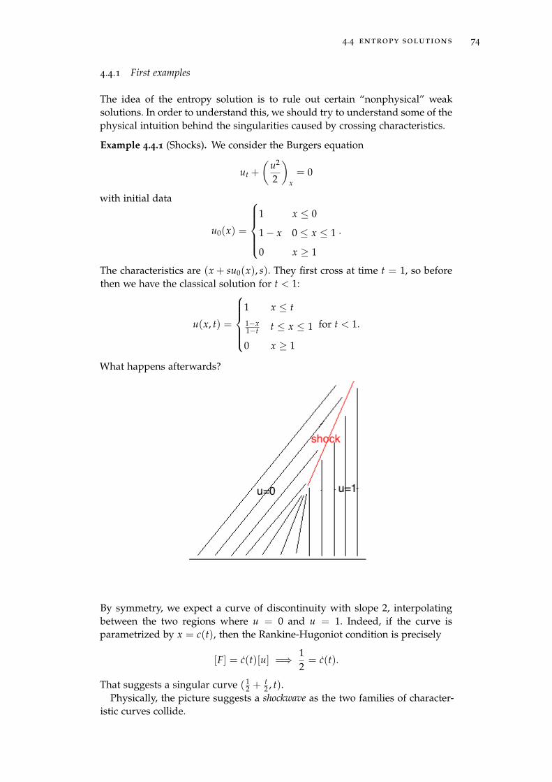
4.4 entropy solutions 74
4.4.1 First examples
The idea of the entropy solution is to rule out certain “nonphysical” weaksolutions. In order to understand this, we should try to understand some of thephysical intuition behind the singularities caused by crossing characteristics.
Example 4.4.1 (Shocks). We consider the Burgers equation
ut +
(u2
2
)x= 0
with initial data
u0(x) =
1 x ≤ 0
1− x 0 ≤ x ≤ 1
0 x ≥ 1
.
The characteristics are (x + su0(x), s). They first cross at time t = 1, so beforethen we have the classical solution for t < 1:
u(x, t) =
1 x ≤ t1−x1−t t ≤ x ≤ 1
0 x ≥ 1
for t < 1.
What happens afterwards?
By symmetry, we expect a curve of discontinuity with slope 2, interpolatingbetween the two regions where u = 0 and u = 1. Indeed, if the curve isparametrized by x = c(t), then the Rankine-Hugoniot condition is precisely
[F] = c(t)[u] =⇒ 12= c(t).
That suggests a singular curve ( 12 +
t2 , t).
Physically, the picture suggests a shockwave as the two families of character-istic curves collide.

4.4 entropy solutions 75
Example 4.4.2 (Rarefaction waves). Now we consider the Burgers equationwith initial condition
u0(x) =
0 x < 0
1 x ≥ 0.
Here the characteristic method fails because the characteristics are “underde-termined.”
One natural way to “fill in” the rest of the characteristics is to vary the slopex/t continuously from 0 to 1.
The solution we have just sketched geometrically has the explicit description
u1(x, t) =
0 x < 0,
1 x > t,xt 0 < x < t.

4.4 entropy solutions 76
Obviously u1 satisfies the Burger equation in the regions x < 0 and x > t. Inthe region 0 < x < t, we can check:
∂u1
∂t+
12
(∂u2
∂x
)2
= − xt2 +
12
( xt
)2
x= 0.
We then only need to check the Rankine-Hugoniot condition on the curvesx = 0 and x = t, but in fact the solution is continuous everywhere, so it isclearly satisfied.
One can also produce a discontinuous Rankine-Hugoniot solution, like whatwe did for the shockwave. If the curve of discontinuity is x(t) = c(t), then theRankine-Hugoniot condition is
12= c(t)
so we have a shockwave along a line of slope 2, as before.
The explicit formula for this solution is
u(x, t) =
0 x < t,
1 x > t.
This solution appears “unphysical” in the sense that there was a shock withoutany physical cause.
4.4.2 Entropy solutions
The idea of entropy solutions is to capture the intuition that the entropy of aphysical system only increases. Suppose Φ(u) is a smooth convex function,which we think of as a measure of entropy for the solution u. Actually, theusual physical entropy functions are concave, so we think of Φ(u) as being thenegative of the entropy.

4.4 entropy solutions 77
Definition 4.4.3. Let Ψ be a smooth function such that
Φ′(u) f ′(u) = Ψ′(u).
Then we call (Φ, Ψ) an entropy/flux pair.
The idea is that for a conservative system
ut + f (u)x = 0
we also have a “conservation of entropy”
Φ(u)t + Ψ(u)x = Φ′(u)ut + Ψ′(u)ux
= − f ′(u)Φ′(u)ux + Ψ′(u)ux
= (Ψ′(u)− f ′(u)Φ′(u))ux
= 0.
In general, when our system can undergo a shock, we don’t necessary requirethat the entropy be conserved, but we expect Φ(u) to decrease (recall that thisis the negative of the physical entropy, which increases). So that correspondsto the condition
Φ(u)t + Ψ(u)x ≤ 0.
Now, this can be measured in a weak sense.We are ready to give the formal definition of entropy solutions. We consider
a PDE of the form
ut + f (u)x = 0 R× [0, T) (32)
u(x) = u0(x) R× 0.
Definition 4.4.4. Suppose f ∈ C1(R) ∩ L∞(R). We say that u ∈ L∞(Ω) is anentropy solution to (32) if for all entropy/flux pairs, we have for all positivefunctions ϕ ∈ C∞
c (R× [0, T)) we have the inequality∫R
∫[0,T)
Φ(u)ϕt + Ψ(u)ϕx dtdx +∫
RΦ(u0(x))ϕ(x, 0) dx ≥ 0. (33)
Remark 4.4.5. 1. Note that the test function must be positive!
2. An alternate formulation is to demand that u(·, t) → g in L1(R) as t →0, and for all positive test functions ϕ ∈ C∞
c (R × [0, T)) we have theinequality ∫
R
∫[0,T)
Φ(u)ϕt + Ψ(u)ϕx dtdx ≥ 0. (34)
This is the definition that Evans uses.
3. It is easy to construct lots of entropy/flux pairs. For any Φ, we can take
Ψ(z) =∫ z
z0
Φ′(w) f ′(w) dw.
For good measure, let’s verify that this solution concept is indeed compatiblewith the ones we already have.
Proposition 4.4.6. A classical solution to (32) is an entropy solution.
4.4 entropy solutions 78
Proof. The argument we gave to motivate the definition already shows that ifu is a classical solution, then we can integrate by parts to deduce that for allϕ ∈ C∞
c (R× [0, T)).∫R
∫[0,T)
Φ(u)ϕt + Φ(u)ϕx +∫
Ru0(x)ϕ(x, 0) = 0
Proposition 4.4.7. An entropy solution to (32) is a weak solution.
Proof. We take the entropy/flux pairs Φ(u) = ±u and Ψ(u) = ±F(u) (orsmooth approximations thereof, if necessary). The definition of entropy solu-tion shows that for all positive ϕ ∈ C∞
c (R× [0, T)), we have∫R
∫[0,T)
(±u)vt + (±F(u))vx dtdx +∫
R±u(x, 0)v(x, 0) dx ≥ 0.
Obviously, this is only possible if both inequalities are in fact equalities.
4.4.3 Viscosity solutions
As we have seen, it may be difficult to solve a PDE of the form in (32). One veryclever approach is the method of vanishing viscosity, which studies the equationperturbed by a “viscosity term”:
uεt + F(uε)x − εuε
xx = 0 R× [0, T) (35)
uε(x) = u0(x) R× 0.
By introducing this second-order term, the equations (35) admit classical (evensmooth) solutions. Intuitively, we expect a “physically correct” solution to ouroriginal problem (32) to be the limit of the smooth solutions uε.
To illustrate this idea, we assume that
1. uε is uniformly bounded for 0 ≤ ε ≤ 1, and
2. uε → u almost everywhere as ε→ 0.
In practice, this second condition is highly nontrivial to verify, but let’s seewhere it leads us. Of course, even if the uε are all smooth, we cannot necessarilydeduce that u will be classical. However, it is easy to show that the limit willstill be a weak solution.
Lemma 4.4.8. Under the assumptions (4.4.3), u is a weak solution to (32).
Proof. Let ϕ ∈ C∞c (R× [0, T)) be a test function. Integrating by parts, we find
that
0 =∫
R
∫[0,T)
(uεt + F(uε)x − εuε
xx)ϕ dtdx
= −∫
R
∫[0,T)
uε ϕt + f (uε)ϕx dtdx−∫
Ru0(x)ϕ(x, 0) dx
ε→0−−→∫
R
∫[0,T)
uϕt + f (u)ϕx dtdx−∫
Ru0(x)ϕ(x, 0) dx
where the limit is justified by dominated convergence.

4.4 entropy solutions 79
The more interesting result is that the limit will be an entropy solution.
Theorem 4.4.9. Under the assumptions (4.4.3), u is an entropy solution to (32).
Proof. Let Φ, Ψ be an entropy/flux pair. Following the calculation we per-formed when introducing the definition of entropy solutions, we find:
Φ(uε)t + Ψ(uε)x = Φ′(uε)uεt + Ψ′(uε)uε
x
= Φ′(uε)(εuεxx − f ′(uε)uε
x) + Ψ′(uε)uεx
= εΦ′(uε)uεxx.
This last term looks like it came from the second derivative of Φ(uε). We com-pute
Φ(uε)xx = (Φ′(uε)uεx)x = Φ′(uε)uε
xx + Φ′′(uε)(uεx)
2.
In particular, since Φ is convex we have Φ(uε)xx ≥ Φ′(uε)uεxx. Now sub-
stituting this above and integrating, we find that for all positive functionsϕ ∈ C∞
c (R× [0, T)), we have∫R
∫[0,T)
Φ(uε)ϕt + Ψ(uε)ϕx +∫
RΦ(u0(x))ϕ(x, 0) = −
∫R
∫[0,T)
(Φ(uε)t + Ψ(uε)x)ϕ
≥ −ε∫
R
∫[0,T)
Φ(uε)xx ϕ
= −ε∫
R
∫[0,T)
Φ(uε)ϕxx.
Now applying the dominated convergence theorem and the assumptions (4.4.3),we deduce that∫
R
∫[0,T)
Φ(uε)ϕt + Ψ(uε)ϕx dtdx +∫
RΦ(u0(x))ϕ(x, 0) dx ≥ 0.
4.4.4 Kruzkov’s Theorem
It turns out that the Cauchy problem (32) is well-posed for entropic solu-tions. This and much more follows from an extremely powerful result calledKruzkov’s Theorem. This is hard even to state completely, let alone prove, so wedescribe only some of the main features.
Theorem 4.4.10 (Kruzkov). Suppose u0 ∈ L∞(R). Then there exists a unique u ∈L∞(R× [0, T)) ∩ C([0, T), L1(R)) solving the PDE (32), and this solution satisfies
||u||L∞(R×[0,T)) = ||u0||L∞(R).
More precisely, suppose u0, v0 ∈ L∞(R) and u, v are the solutions with these respec-tive initial data. Let M = sup| f ′(x)| : x ∈ [inf(u0, v0), sup(u0, v0). Then for allt > 0 and every interval [a, b] we have∫ b
a|v(x, t)− u(x, t)| dx ≤
∫ b+Mt
a−Mt|v0(x, t)− u0(x, t)| dx
and also ∫R
v(x, t)− u(x, t) dx =∫
Rv0(x)− u0(x) dx (36)
4.4 entropy solutions 80
We will sketch a proof of the inequality∫ b
a|v(x, t)− u(x, t)| dx ≤
∫ b+Mt
a−Mt|v0(x, t)− u0(x, t)| dx. (37)
and also (36). By taking the limit over a, b we obtain
||v(·, t)− u(·, t)||L1(R) ≤ ||v0 − u0||L1(R)
which immediately implies uniqueness.
Remark 4.4.11. The equation (37) exhibits a fundamental property of the trans-port equation (and hyperbolic equations more generally), which is finite speedof propagation. One manifestation of this is the following.
Corollary 4.4.12. In the notation above, if u0 has support in [−B, B] then u(t, ·) hassupport in [−B−Mt, B + Mt].
Proof. If [a′, b′] is an interval disjoint from [−B − Mt, B + Mt], then we mayassume without loss of generality that b′ ≤ −B−Mt. Then b′ + Mt ≤ −B, so(37) with v ≡ 0 and v0 ≡ 0 implies that∫ b′
a′|u(x, t)| dx ≤
∫ b′+Mt
a′−Mt|u0(x)| dx = 0.
Now for the proof of (37). To begin, we choose some special entropy/fluxpairs. Imagine that we could take the entropy Φ(z) = |z − α| (it is convexand continuous, but not differentiable in the classical sense). Then Φ′(z) =
sgn(z− α), and
Ψ(z) =∫ z
αΦ′(w)F′(w) dw = sgn(z− α)(F(z)− F(α)).
This isn’t strictly justified, but by approximating |z− α| with a smooth functionwe deduce the following.
Lemma 4.4.13. If u is an entropic solution, then for any k ∈ R and positive ϕ ∈C∞
c (R× [0, T)) we have∫R
∫[0,T)
ϕt|u− k|+ ϕx( f (u)− f (k)) sgn(u− k) dtdx+∫
R|u0(x)− k|ϕ(x, 0) dx ≥ 0.
In fact, the implication goes both ways: a solution is entropic if it satisfies theabove inequality for all k and ϕ. This is essentially because we can approximateany convex function with piecewise linear functions.
The key technical step is to enhance this up by replacing k with v. Let Ω =
R× [0, T).
Proposition 4.4.14. Let u and v be entropy solutions of (32) with initial data u0 andv0. For all positive ϕ ∈ C∞
c (R× [0, T)), we have∫Ω|u− v|ϕt +( f (u)− f (v)) sgn(u− v)ϕx dtdx+
∫R|u0(x)− v0(x)|ϕ(x, 0) dx ≥ 0.

4.4 entropy solutions 81
Proof. Choose a positive function η ∈ C∞c (Ω × Ω). We apply Lemma 4.4.13
with respect to α = v(y, s) and test function η(·, ·, y, s). We then apply Lemma4.4.13 again reversing the roles of u and v, and with test function η(x, t, ·, ·).Summing the results, we have
0 ≤∫ ∫ ∫ ∫
|u(x, t)− v(y, s)|(ηt + ηs)(x, t, y, s)
+∫ ∫ ∫ ∫
sgn(u(x, t)− v(y, s))( f (u(x, t))− f (v(y, s)))(ηx + ηy)(x, t, y, s)
+∫ ∫ ∫
|u0(x)− v(y, s)|η(x, 0, y, s) +∫ ∫ ∫
|u(x, t)− v0(y)|η(x, t, y, 0)
Now we choose η to approximate ϕ(x, t)δ(x − y, t− s), so that the inequalitytends to
0 ≤∫ ∫
|u− v|ϕt + sgn(u− v)( f (u)− f (v))ϕx +∫
R|u0(x)− v0(x)|ϕ(x, 0)
which is the claimed result.
Now we are about ready to complete the proof of the estimate (37). By trans-lating, we may reduce to the case where a = −b. Let T be the trapezoid
T = (x, t) ∈ Ω : − b−M(s− t) < x < b + M(s− t).
Let χ(t) be a smooth, positive cutoff function which is 1 for t < s and sup-ported in t < s + b/M. Let θ(x) be a smooth, positive cutoff function which
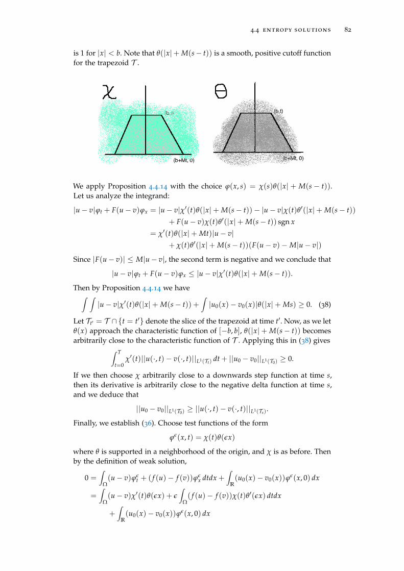
4.4 entropy solutions 82
is 1 for |x| < b. Note that θ(|x|+ M(s− t)) is a smooth, positive cutoff functionfor the trapezoid T .
We apply Proposition 4.4.14 with the choice ϕ(x, s) = χ(s)θ(|x| + M(s − t)).Let us analyze the integrand:
|u− v|ϕt + F(u− v)ϕx = |u− v|χ′(t)θ(|x|+ M(s− t))− |u− v|χ(t)θ′(|x|+ M(s− t))
+ F(u− v)χ(t)θ′(|x|+ M(s− t)) sgn x
= χ′(t)θ(|x|+ Mt)|u− v|+ χ(t)θ′(|x|+ M(s− t))(F(u− v)−M|u− v|)
Since |F(u− v)| ≤ M|u− v|, the second term is negative and we conclude that
|u− v|ϕt + F(u− v)ϕx ≤ |u− v|χ′(t)θ(|x|+ M(s− t)).
Then by Proposition 4.4.14 we have∫ ∫|u− v|χ′(t)θ(|x|+ M(s− t)) +
∫|u0(x)− v0(x)|θ(|x|+ Ms) ≥ 0. (38)
Let Tt′ = T ∩ t = t′ denote the slice of the trapezoid at time t′. Now, as we letθ(x) approach the characteristic function of [−b, b], θ(|x|+ M(s− t)) becomesarbitrarily close to the characteristic function of T . Applying this in (38) gives∫ T
t=0χ′(t)||u(·, t)− v(·, t)||L1(Tt) dt + ||u0 − v0||L1(T0) ≥ 0.
If we then choose χ arbitrarily close to a downwards step function at time s,then its derivative is arbitrarily close to the negative delta function at time s,and we deduce that
||u0 − v0||L1(T0) ≥ ||u(·, t)− v(·, t)||L1(Ts).
Finally, we establish (36). Choose test functions of the form
ϕε(x, t) = χ(t)θ(εx)
where θ is supported in a neighborhood of the origin, and χ is as before. Thenby the definition of weak solution,
0 =∫
Ω(u− v)ϕε
t + ( f (u)− f (v))ϕεx dtdx +
∫R(u0(x)− v0(x))ϕε(x, 0) dx
=∫
Ω(u− v)χ′(t)θ(εx) + ε
∫Ω( f (u)− f (v))χ(t)θ′(εx) dtdx
+∫
R(u0(x)− v0(x))ϕε(x, 0) dx

4.4 entropy solutions 83
Since | f (u)− f (v)| ≤ M|u− v|, each term above is uniformly integrable, so wecan take limit ε→ 0 inside the integrals to obtain∫
Ω(u− v)χ′(t) dxdt + χ(0)
∫R(u0 − v0) dx = 0.
Choosing χ to approximate a step function at time s, so that χ′ approximates−δ(t− s), we deduce (36).
4.4.5 Rankine-Hugoniot type conditions
Let us consider writing down a Rankine-Hugoniot type condition for entropicsolutions. Adopting the notation from §4.3.2, we have for all positive test func-tions ϕ ∈ C∞
c (Ω),
0 ≤∫
ΩϕtΦ(u) + ϕxΨ(u)
=
(∫Ωl
+∫
Ωr
)ϕtΦ(u) + ϕxΨ(u)
= −(∫
Ωl
+∫
Ωr
)(Φ(u)t + Ψ(u)x)ϕ +
∫Γ(Ψ(u), Φ(u)) · nl ϕ
≤∫
Γ([Ψ(u)], [Φ(u)]) · nl ϕ.
Since this holds for all positive test functions, we may conclude that
[Ψ(u)]nx + [Φ(u)]nt ≥ 0.
If our curve Γ is parametrized by x(t) = η(t), then we may take nl ∝ (1,−η(t)).Setting σ = η as before, we can reformulate the condition as
σ[Φ(u)] ≤ [Ψ(u)].
By taking Φ(u) to approximate |u− α| for any constant α, we have
[( f (u)− f (α)) sgn(u− α)] ≤ σ[|u− α|].
(The same trick was used in Lemma 4.4.13.) Recall that it turns out that thisfamily of inequalities is also sufficient.
Consider this inequality at a point of Γ where ul 6= ur. By choosing α verysmall, sgn(ul − α) = sgn(ur − α) is constant at this point andd we deduce that
σ =[ f (u)][u]
.
By choosing α in the interval [ul , ur], say α = τul +(1− t)ur for some τ ∈ (0, 1),we (eventually) deduce that
((1− τ) f (ul) + τ f (ur)− f ((1− τ)ul + τur)) sgn(ul − ur) ≥ 0.
Therefore, we have two cases.
1. If ul < ur, then f restricted to [ul , ur] must lie above its chord.
2. If ul > ur, then f restricted to [ur, ul ] must lie below its chord.

4.4 entropy solutions 84
This rules out the “nonphysical” weak solution we found earlier for the Burg-ers equation in Example 4.4.2.
A further consequence of the inequality is that
f ′(ul) ≥ σ ≥ f ′(ur)
which is called Lax’s entropy condition. Physically, this means that the char-acteristics intersecting along Γ cannot emerge from Γ, but must emanate frompoints “in the past” (again, contrast this with the solution u2 from Example4.4.2). If the inequalities are strict, as is the case when f is strictly convex orconcave, then it means that the entropy solution can be calculated by the method ofcharacteristics.
4.4.6 Riemann Problems
The Riemann problem is a special Cauchy problem with initial data of the form
u0(x) =
ul x < 0,
ur x > 0.(39)
The point is that the solutions are invariant under homotheties (x, t) 7→ (ax, at).More generally, if u(x, t) is the entropy solution for u0(x), then u(ax, at) is theentropy soultion for u0(ax). Therefore, the solutions are of the form u(x, t) =v(x/t). When does this satisfy (32)? We calculate
∂tv(x/t) + ∂xF(v(x/t)) = v′(x/t)(− x
t2
)+ F′(v(x/t))v′(x/t)
1t
= v′(x/t)(
F′(v(x/t))− x/t)
.
Therefore, if v′(x/t) 6= 0 we have F′(v(x/t)) = x/t, hence v = (F′)−1.

4.4 entropy solutions 85
Theorem 4.4.15. Suppose f is strictly convex and C2. Then the unique entropy solu-tion of the Riemann problem (32) with initial data (39) is given as follows.
1. If ul > ur, then
u(x, t) =
ulxt < σ,
urxt > σ
where σ = f (ul)− f (ur)ul−ur
.
2. If ul < ur, then
u(x, t) =
ul
xt < f ′(ul),
v( xt ) f ′(ul) <
xt < f ′(ur),
urxt > f ′(ur).
where v(x) = ( f ′)−1(x).
Example 4.4.16. Consider the Burgers equation again, with initial data
u0(x) =
0 x < 0
1 0 ≤ x ≤ 1,
0 x > 1.
For t ≤ 2, the entropic solution can be found by juxtaposing the entropicsolutions we found in Example 4.4.1 and Example 4.4.2.
What happens at t = 2? From the diagram we see that the rarefaction curvefrom the origin meets the shock curve from (1, 0), forming another shock curve(x(t), t). What is this curve? We have
x(t) = σ =[F(u)][u]
=12 (x/t)2
(x/t)=
x2t
=x(t)
t.
Solving, we find that x(t) = (2t)1/2. Therefore, the solution for t ≥ 2 is
u(x, t) =
0 x < 0,xt 0 < x < (2t)1/2
0 x > (2t)1/2
.

5T H E WAV E E Q U AT I O N
5.1 introduction to the wave equation
The wave equation in n + 1 dimensions is
∂2t u− ∂2
1u− . . .− ∂2nu = 0. (40)
where u = u(t, x) and x = (x1, . . . , xn). We write = ∂2t − ∂2
1− . . .− ∂2n, which
is called the d’Alembertian operator. The wave equation has a distinguished timedirection, so we write R` = R1+n to emphasize this.
We can think of the wave equation as a system of linear transport equations.Indeed, consider for the moment the case n = 1. Observe that we can factorizethe “difference of squares”
∂2t u− ∂2
xu = 0. (41)
If we write v = (u, ∂tu− ∂xu) =: (v1, v2) then the PDE (41) is equivalent to thesystem
∂tv1 + ∂xv1 = v2
∂tv2 − ∂xv2 = 0.
In higher dimensions, one writes down an operator Dx =√−∆x and converts
(40) into the system
∂tv1 + iDxv1 = v2
∂tv2 + iDxv2 = 0.
For this reason, the wave equation behaves like a linear hyperbolic equation,even though it has degree 2. The construction of the operator Dx is nontriv-ial; one of Dirac’s great insights was to construct this using spinors in R1+3,leading to the Dirac equation.
5.2 second-order hyperbolic equations
In contrast to elliptic equations, hyperbolic equations have “as many character-istic hypersurfaces as possible.” We will focus on a specific class of hyperbolicequations of the form
−∂2t + Pu = f (0, T)×Ω, (42)
u = 0 ∂[0, T]×Ω,
u = u0 0×Ω,
∂t = u1 0×Ω.
where
Pu = −n
∑i,j=1
∂j(aij(t, x)∂iu) +n
∑i=1
bi(t, x)∂iu + c(t, x)u.
86

5.3 energy estimates 87
Here Ω ⊂ Rn is an open subset. Although this appears to be a Cauchy problem,it has Dirichlet conditions on the spatial boundary.
Definition 5.2.1. We say that the PDE (42) is hyperbolic if P is elliptic, i.e. for all(t, x) ∈ [0, T]×Ω and ξ ∈ Rn we have
n
∑i,j=1
aij(t, x)ξiξ j > 0.
We say that it is uniformly elliptic if there exists some uniform constant θ suchthat
n
∑i,j=1
aij(t, x)ξiξ j > θ|ξ|2.
Said differently, the principal symbol for the equation is a quadratic form ofsignature (n, 1).
The set 0×U is non-characteristic for the PDE (42) (and these are the onlynon-characteristic points) so we might expect well-posedness for this Cauchyproblem. The Cauchy-Kovalevskaya theorem guarantees local existence of an-alytic solutions given analytic initial data.
5.3 energy estimates
5.3.1 Homogeneous equation
We now return to the wave equation u = f , and perform some a prioriestimates. These are useful in establishing existence and uniqueness; for nowwe just assume sufficient regularity and decay to justify the calculations. Forsimplicity, we work on Ω = Rn.
Multiply the equation (40) by ∂tu and integrate:
0 =∫
Rn
∫ T
0∂tu(∂2
t u− ∆xu) dtdx
=∫
Rn
∫ T
0∂tu(
12
u2t
)− ∂tu(∇x · ∇xu) dtdx
=∫
Rn
∫ T
0∂t
(12
u2t
)+ [∂t(∇xu) · ∇xu] dtdx +
∫Rn
∂tu(∇xu · n) dx
=∫
Rn
∫ T
0∂t
(12
u2t
)+ ∂t
∣∣∣∣12∇xu∣∣∣∣2 dtdx +
∫Rn
∂tu(∇xu · n) dx
=∫
Rn
[12
u2t +
12|∇xu|2
]T
0+∫
Rn∂tu(∇xu · n) dx
Assuming that ∂tu = u1 vanishes along t = 0, we see that the function
E(t) :=∫
Rn
12
ut(x, t)2 +12|∇xu(x, t)|2 dx
is constant in time. This is already enough to imply the uniqueness of solutionsto the wave equation.

5.3 energy estimates 88
5.3.2 Local Energy Estimates
We now develop some local estimates that reveal a cone of dependence, like whatwe found in Kruzkov’s Theorem. We define the cone
C =⋃t≤T
t × B(x0, R + T − t).
Let Ct = t × B(x0, R + T − t) denote the slice at time t. We define the localenergy
E(t) :=∫Ct
12|ut(t, x)|2 + 1
2|∇xu(t, x)|2 dx.
We assume enough regularity and decay so that this is well-defined. Then wehave
dE(t)dt
=ddt
∫Ct
12|ut|2 +
12|∇xu|2 dx
=∫Ct
uttut − ∂t∇xu · ∇xu dx−∫
∂Ct
12|ut(t, x)|2 + 1
2|∇xu(t, x)|2 dσ.
Integrating the second term by parts, we find that∫Ct
∂t∇xu · ∇xu dx =∫
∂Ct
∂tu(∇xu · n) dσ−∫Ct
∂tu∆xu dx.
Substituting this above, we find that
dE(t)dt
=∫Ct
ut(utt − ∆xu) dx +∫
∂Ct
∂tu(∇xu · n)− 12|ut(t, x)|2 + 1
2|∇xu(t, x)|2 dσ
=∫
∂Ct
∂tu(∇xu · n)− 12|ut(t, x)|2 + 1
2|∇xu(t, x)|2 dσ.
By Cauchy-Schwarz,
|∂tu(∇xu · n)| ≤ |∂tu||∇xu| ≤ 12|ut(t, x)|2 + 1
2|∇xu(t, x)|2,
so we see thatdE(t)
dt≤ 0.
Therefore, for any time 0 < t < T we have
E(T) ≤ E(0).
Note that this implies “finite speed of propagation” as we saw in the transportequation. If the initial data is supported in some set, then at all times thesoution will be supported in a “light cone” emanating from that set.


