APPLICATIONS OF MARKOV CHAIN MONTE CARLO AND POLYNOMIAL CHAOS EXPANSION BASED TECHNIQUES FOR STATE AND PARAMETER ESTIMATION An Undergraduate Research Scholars Thesis by SHUILIAN XIE Submitted to Honors and Undergraduate Research Texas A&M University in partial fulfillment of the requirements for the designation as UNDERGRADUATE RESEARCH SCHOLAR Approved by Research Advisor: Dr. Krishna R. Narayanan May 2014 Major: Electrical Engineering
Transcript
APPLICATIONS OF MARKOV CHAIN MONTE CARLO AND
POLYNOMIAL CHAOS EXPANSION BASED TECHNIQUES
FOR STATE AND PARAMETER ESTIMATION
An Undergraduate Research Scholars Thesis
by
SHUILIAN XIE
Submitted to Honors and Undergraduate ResearchTexas A&M University
in partial fulfillment of the requirements for the designation as
UNDERGRADUATE RESEARCH SCHOLAR
Approved byResearch Advisor: Dr. Krishna R. Narayanan
APPLICATIONS OF MARKOV CHAIN MONTE CARLO AND POLYNOMIAL CHAOSEXPANSION BASED TECHNIQUES FOR STATE AND PARAMETER ESTIMATION .
(May 2014)
SHUILIAN XIEDepartment of Electrical and Computer Engineering
Texas A&M University
Research Advisor: Dr. Krishna R. NarayananDepartment of Electrical and Computer Engineering
In this research thesis, we implement Markov Chain Monte Carlo techniques and polynomial-
chaos expansion based techniques for states and parameters estimation in hidden Markov
models (HMM). Our goal is to estimate the probability density function (PDF) of the states
and parameters given noisy observations of the output of the hidden Markov model. We
consider three problems, namely, (i) determining the PDF of the states in a non-linear
HMM using sequential MCMC techniques, (ii) determining the parameters of discretized
linear, ordinary differential equations (ODE) given noisy observations of the solutions and
(iii) Determining the PDF of the solution of a linear ordinary differential equation when the
parameters of the ODE are random variables. While these problems naturally arise in several
areas in engineering, this thesis is motivated by potential applications in bio-mechanics. One
of the interesting research questions that is being considered by some researchers is whether
the formation of clots can be predicted by observing the mechanical properties of arteries,
such as their stiffness. In order for this approach to be successful, it is critical to estimate
the stiffness of arteries based on noisy measurements of their mechanical response. The
parameters of these models can then be used to differentiate diseased arteries from healthy
ones or, the parameters can be used to predict the probability of formation of plaques. From
experimental data, we would like to infer the posterior density of the states and parameters
1
(such as stiffness), and classify it as being healthy or diseased. If it is accomplished, this will
improve the state-of-the art in modeling mechanical properties of arteries, which could lead
to better prediction, and diagnosis of coronary artery disease.
2
DEDICATION
I dedicate my undergraduate research work to my family and many friends. A special feeling
of gratitude to my loving parents who support me to study at Texas A&M University. My
sisters Lulu and Jinping have never left my side.
I also dedicate this research work to my friends, without whose help, I could not have been
motivated and positive. I will always appreciate all they have done, especially Xintong Xia
and Shan Wang for helping me develop my strong heart and optimistic altitude.
3
ACKNOWLEDGMENTS
First and foremost, I would like to take this opportunity to express my deepest gratitude to
my research advisor, Dr. Krishna R. Narayanan, for providing me a great opportunity to
learn about statistical signal processing. Ever since the first days when he taught me Digital
Communication, Krishna has been an outstanding mentor and role-model. His enthusiasm
for research and teaching is inexhaustible. His brilliant insight, patient guidance throughout
my senior year helped to lit my route of future study. Working with him was indeed a
pleasant and rewarding experience. Without his continuous support, my undergraduate
research would have never become possible.
I would also like to thank Dr. Arun R. Srinivasa, a professor in Department of Mechanical
Engineering at Texas A&M University. Dr. Srinivasa provided a bunch of profound insights
and helpful resource to our project.
Furthermore, I’m very grateful to all the graduate students under Dr. Krishna Narayanan’s
advisory, especially Avinash Vem, who offered great help for my research project.
Last, I want to thank the Department of Electrical and Engineering, Texas A&M University
for providing me a platform to pursue my research interest and giving me award to honor
my research achievements as an undergraduate. Additionally, I would like to appreciate Dr.
Narayanan’s funding support, which helped ease my financial burdens.
4
NOMENCLATURE
MCMC Markov Chain Monte Carlo
Ns Particle Number
PCE Polynomial Chaos Expansion
PDF Probability Density Function
SIS Sequential Importance Sampling
SIR Sequential Importance Resampling
SMC Sequential Markov Chain
5
CHAPTER I
INTRODUCTION
We consider three closely-related problems in statistical signal processing in this thesis.
These problems pertain to inferring the posterior distribution of the states or parameters of
a discrete-time hidden Markov model given noisy observations of the output of such a model.
More specifically, we consider the following discrete-time hidden Markov model
xk = fk (xk−1, θk) + vk−1 (I.1)
zk = gk(xk) + nk (I.2)
where xk and zk denote the state and observation at time instant k, respectively. θk is a
vector of parameters and vk and nk denote i.i.d noise sequences.
The following three problems are considered. (i) Estimating the probability density function
(PDF) of xk given observations zks, (ii) Estimating the PDF of the parameters θk given
observations zks and (iii) Estimating the PDF of zks given the PDF of θks. Two main
techniques are used to accomplish these tasks. We use Markov chain monte carlo techniques
to accomplish tasks (i) and (ii) and we use polynomial-chaos based expansion techniques to
accomplish task (iii).
While hidden Markov models and the aforementioned estimation problems naturally occur in
several engineering applications, the study in this thesis is mainly motivated by applications
in bio-mechanics. The broader context within which this study was undertaken is described
below. Currently, there is interest within the bio-mechanics research community to answer
the question of whether the mechanical properties of arteries can be used to predict the
formation of arterial plaques. An important first step in addressing this question is to find
a mathematical model that explains the mechanical behavior of the artery. In particular, if
6
we can conduct an experiment (on dead tissue) where we apply a combination of forces and
torques and measure the expansion of the artery, can we then fit a mathematical model that
will explain the response of the artery? Current modeling methods in biomechanics largely
assume that the expansion of the artery is a deterministic function of the input force and
try to find models, typically the shape of the artery is given by the solution to a differential
equation. It is true that such deterministic models have been very successful in modeling
man-made materials. However, using such deterministic models to obtain biomechanics
models has failed because there is no simple one to one relationship between the parameters
of the model and measured values. In addition, there is huge variation in the response from
one tissue sample to the other. Our approach is to model the unknown parameters (e.g.
elasticity) as random variables and obtain stochastic models for the arterial response.
More specifically, we will assume that the shape of the artery is the solution to a (possibly
non-linear) differential equation whose parameters are unknown. Further, from experiments,
we can observe the shape of the artery either entirely or partially in the presence of some
measurement noise. When this model is appropriately discretized, it can be seen that the
resulting model falls in the framework of a hidden Markov model as given in equations (I.1)
and (I.2).
Performing the estimation task described above is not an easy because the underlying mod-
els are often non-linear. The objective of this project is to explore two powerful ideas in
statistical signal processing to carry out these estimation tasks. The first one is the idea
of Markov Chain Monte Carlo (MCMC) methods [1],[2]. The second one is the idea of
using polynomial-chaos based model fitting [3]. We believe that these will be powerful, effec-
tive and feasible ways to perform estimation tasks in the presence of non-linearities and/or
unknown parameters.
An important consequence of being able to perform these estimation tasks well is that the
results of estimation can be used for diagnostic purposes. For example, if one can obtain
the distribution of the unknown parameters from experimental data, this can be used to
7
classify the artery as being healthy or diseased or the likelihood of the artery developing
into a diseased artery can be estimated. Even though these classification problems are not
addressed in this thesis, the estimation step can be seen to be crucial for the classification
problem.
The rest of the thesis is organized as follows. In Chapter II, we discuss sequential monte carlo
techniques, in particular, the particle filtering technique for estimating the states of a HMM.
We discuss the degeneracy problem associated with naive particle filtering techniques and we
consider improved sampling techniques based on resampling. The algorithms considered in
this chapter are based on those in [5]. In Chapter III, we consider the problem of estimating
unknown parameters of a linear ordinary differential equation by observing a noisy version
of the output of the differential equation. We discuss why traditional sequential monte carlo
techniques are not well-suited for this problem. We implement a kernel-smoothing based
sequential monte carlo technique based on [6] for the estimating the parameters. We discuss
the limitations of such a scheme for the problem that we studied. Finally in Chapter IV, we
consider the use of polynomial-chaos based expansion techniques for estimating the PDF of
the output of a linear ODE, when the parameters in the ODE are random variables. We
implement this scheme to estimate the PDF of the output of a first-order ODE. Chapter V
discusses some future work that can be performed to continue research along the direction
of research considered in this thesis.
8
CHAPTER II
STATE ESTIMATION USING MARKOV CHAIN MONTE
CARLO METHODS
Problem Statement
Consider a hidden Markov state-space model given by
xk = fk (xk−1, θ) + vk (II.1)
zk = gk (xk) + nk (II.2)
where (II.1) and (II.2) give the state xk and the observation zk at time instant k, respectively.
Note that vk and nk denote i.i.d noise sequences. We wish to determine the posterior pdf
of xk given the observations zT0 , where zT0 denotes the vector {zk, i = 0, .., T} and T is the
maximum time for which observations are available. This is a special case of (I.1) and (I.2)
with θ being fixed.
Is is well known that the Kalman filter is optimal for determining the posterior pdf under
the following conditions:
• vk and nk are drawn from Gaussian distribution of known parameters.
• fk (xk−1, θ) is known and is a linear function of xk−1.
• gk (xk) is a known linear function of xk.
However, when the noise sequences are not Gaussian, nor f and g are linear, the Kalman filter
is not an optimal solution for this tracking. In this case, sequential monte carlo approaches
have been very successful for the estimation of states xks. [5]
9
Sequential Monte Carlo Approach for Estimation of States-SIS
The Sequential Importance Sampling (SIS) Particle Filter is a Monte Carlo method that is
used for states and parameters estimation. In this approach, we use {xik} and a corresponding
set of weights wik to characterize the posterior density pdf p (x|z). The key idea of this
approach is to represent the pdf by these random samples xik with associate weights wik,
under the noisy measurements zks. In the SIS algorithm, the random sample xi0:k are drawn
from (II.1), which shows the relationship between the previous state and current state. The
next step is to assign the particle a weight. The weights are updated according to
wik ∝p (zk|xik) p
(xik|xik−1
)q(xik|xi0:k−1, z1:k
) . (II.3)
where q(xik|xi0:k−1, z1:k
)is called the proposal density function, and we can choose q
(xik|xi0:k−1, z1:k
)to be anything that is easy to sample from. To simplify our problem, we define
q(xik|xi0:k−1, z1:k
), p
(xik|xik−1
). (II.4)
so that it follows that
wik ∝ wik−1p(zk|xik
). (II.5)
The weights wik are normalized such that∑
iwik = 1.
Once we get the random measure[{xik, wik}
Ns
i=1
], we can calculate the posterior filtered density
p (xk|z1:k) as
p (xk|z1:k) ≈Ns∑i=1
wikδ(xk − xik
)(II.6)
It can be shown that as Ns →∞, the approximation approaches the true posterior density.[5]
A pseudocode for the algorithm is presented below:
Algorithm 1: Sequential Important Sampling (SIS) Particle Filter [5][{xik, wik}
Ns
i=1
]= SIS
[{xik−1, w
ik−1}Ns
i=1
]
10
• FOR i = 1 : Ns
– Draw xik ∼ q(xk|xik−1, zk
)– Assign the particle a weight, wik ∝ wik−1
p(zk|xik)p(zk|xik−1)q(xik|xik−1,zk)
where q(xik|xik−1, zk
)is called the proposal density function
• END FOR
Sequential Monte Carlo Approach for Estimation of States-SIR
After the implementation of SIS, we find that there are some negligible weights whose con-
tribution to p (xk|z1:k) is almost zeros. When this happens, small weights take a large
computational effort to update; however they do not contribute substantially to the overall
pdf. This is called degeneracy problem. In order to solve this problem, it is common to
use resampling algorithm. The basic idea of resampling is to eliminate particles that have
small weights and to concentrate on particles with large weights. In the algorithm, we firstly
construct a CDF of the weights. To determine whether the weight is small or large, we
utilized a vector called uj, shown in the resampling algorithm below. If uj is less than the
value of CDF, we regard the corresponding weight large and then assign a new weight as 1Ns
.
Otherwise, we can say that the weight is small enough to eliminate. Therefore, we could see
that resampling involves generating a new set weights wik as 1Ns
A pseudo code for the algorithm is presented:
Algorithm 2: Resampling Algorithm[5][{xj∗k , w
j∗k , i
j}Ns
i=1
]= RESAMPLE
[{xik−1, w
ik−1}Ns
i=1
]• Initialize the CDF: c1 = 0
• FOR i = 2 : Ns
– Construct CDF: ci = ci−1 + wik
• END FOR
• Start at the bottom of the CDF: i = 1
11
• Draw a starting point: u1 ∼ U[0, 1
Ns
]• FOR j = 1 : Ns
– Move along the CDF: uj = u1 + 1Ns
(j − 1)
– WHILE uj ≥ ci
∗ i = i+ 1
– END WHILE
– Assign sample: xj∗k = xik
– Assign weight: wjk = 1Ns
– Assign parent: ij = i
• END FOR
Sequential Importance Resampling (SIR) Algorithm is a combination of SIS and Resampling
algorithm, which means that we firstly obtain the random measure[{xik, wik}
Ns
i=1
], and then
implement resampling algorithm to generate a new set of the random measure[{xj∗k , w
ik
}Ns
i=1
].
After that, we get the posterior filtered density p (xk|z1:k), which is showed in the previous
section.
Results of MCMC method in estimation of states
Example 1 We consider the estimation of xk by the SIS algorithm for the following example:
xk =xk−1
2+
25xk−11 + x2k−1
+ 8 cos (1.2k) + vk−1 (II.7)
zk =x2k20
+ nk
where vk and nk are zero mean Gaussian random variables with variance 10 and 1, respec-
tively. We consider 1,000 particles and time up to 50 units. The value of x0 is drawn
uniformly between -25 and 25. Fig II.1 presents the tracking of the states xk as time, which
we call the estimation of posterior density function of xk. Red dots mean there are higher
12
possibility for xk to fall into corresponding small interval. Fig II.2 shows the true value of
xk versus time k. We could mainly see that as time becomes larger, the estimation is more
accurate. The posterior density function shows the effectiveness of Sequential Importance
Sampling algorithm. Besides, calculating the Root Mean Squared Error (RMSE) can also
represent the performance of sequential monte carlo filter. Where
RMSE =
√√√√ T∑k=1
(xk − xik)2wik (II.8)
From above equation, we could compute the RMSE of SIS is about 6.83.
Due to degeneracy problem of SIS, we implement another algorithm, Sequential Importance
Resampling. Fig II.3 presents the tracking of the states xk as time, which we call the
estimation of posterior density function of xk. Fig II.4 shows the true value of xk versus
time k. we would see the SIR method also works well. Also, we compute the RMSE of SIR,
which is about 5.69.
13
Fig. II.1.: The posterior density function of xk by SIS
Fig. II.2.: The plot of the true value of xk vs k
14
Fig. II.3.: The posterior density function of xk by SIR
Fig. II.4.: The plot of the true value of xk vs k
15
Conclusion
In this chapter we showed that Markov chain monte carlo methods can be very effective
for state estimation in hidden Markov models. Our simulation results shows that after an
initial period, the particle filtering algorithm is able to track the states well. Resampling is
an effective technique to deal with the degeneracy problem. By concentrating the updating
effort on large weights, the resampling technique is able to decrease the estimation error.
16
CHAPTER III
PARAMETER ESTIMATION USING MARKOV CHAIN
MONTE CARLO METHOD
Problem Statement
The previous chapter deals with the state estimation when the parameter θ is being fixed. In
this chapter, we mainly focus on the estimation of parameter θ. Again, we assume a Hidden
Markov model given by
yk = fk (yk−1, θ) + vk (III.1)
zk = gk (yk) + nk (III.2)
where (III.1) and (III.2) give the state yk and the observation zk at time instant k, respec-
tively. Note that vk and nk denote i.i.d noise sequences. In this problem, we are going to
deal with the estimation of posterior density function of θ.
Kernel Smoothing Algorithm
The combination of Kernel Smoothing Algorithm and particle has been shown to work well in
some cases. Suppose we have {yik, θik}, and associated weights {wik} that together represent
a monte carlo importance sample. We can see that the weights wik are able to represent the
probability density function of θ.
The basic idea is to regard θ as time-varying with small random perturbations[6]. One way
is to add an independent, zero-mean normal increment to the parameter at each time. That
is,
θk+1 = θk + ζk+1 (III.3)
ζk+1 ∼ N (0,Wk+1)
17
where Wk+1 is independent with given states and observations.
When updating θik, we computer the new sample as N(m
(k)k , h2Vk
), where m
(k)k is called the
locations of θ, shown as the algorithm below, and h is chozen to make the new sample more
concentrated about to their locations. In terms of corresponding weights wik, we have the
same method shown as SIS algorithm, that is
wik ∝ wik−1p(zk|yik
). (III.4)
The weights wik are normalized such that∑
iwik = 1.
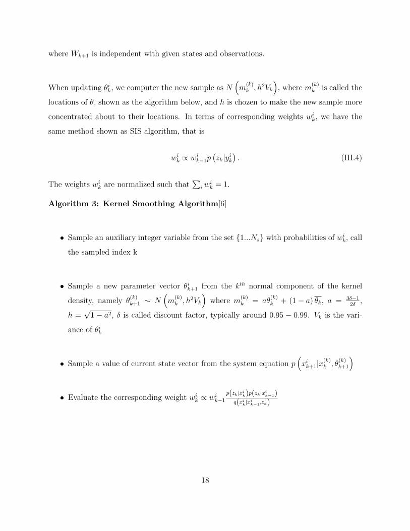
Algorithm 3: Kernel Smoothing Algorithm[6]
• Sample an auxiliary integer variable from the set {1...Ns} with probabilities of wik, call
the sampled index k
• Sample a new parameter vector θik+1 from the kth normal component of the kernel
density, namely θ(k)k+1 ∼ N
(m
(k)k , h2Vk
)where m
(k)k = aθ
(k)k + (1− a) θk, a = 3δ−1
2δ,
h =√
1− a2, δ is called discount factor, typically around 0.95 − 0.99. Vk is the vari-
ance of θik
• Sample a value of current state vector from the system equation p(xik+1|x
(k)k , θ
(k)k+1
)
• Evaluate the corresponding weight wik ∝ wik−1p(zk|xik)p(zk|xik−1)q(xik|xik−1,zk)
18
Results of MCMC Method in Estimation of Parameter
Example 2 In this example, We have the following model:
yk+1 = yk + ykθ∆ (III.5)
zk = yk + nk
In our experiment, to generate the observations, we set the value of θ as -0.2. During
the estimation step, we set the number of particles Ns as 10,000 and time T as 200. Fig
III.1 has four subfigures, the first one shows the distribution of θ when k = 1, and from
the figure, we can see that the values of θ are around a fixed value as -0.2. The rest of
subfigures also have shown the estimated θ is a true distribution. Fig III.2 is a histogram
showing the distribution of θ when k = T . From these two figures, we can see that during
the implementation of Kernel Smoothing Algorithm, θs are approaching to a certain value,
which shows the effectiveness of this method to estimate parameters.
Discussion of this example: When we implemented this algorithm, we found that when
∆ is very small, say 0.01, the estimated θ will concentrate to a random number between -1
and 0, instead of a fixed number. We believe the reason for this is as follows: when ∆ is
very small, the truly estimated value of θ will not affect the first few steps of evolution of
θ, especially when we utilize resampling to make estimated θ more concentrated to “wrong”
θ, which is a random value between -1 and 0. In addition, the joint estimation does not
produce results consistently. This is because the correct deduction of next state from the
current state should be
yk+1
(θik+1
)= yk
(θik)
+ yk(θik)
∆θik+1 (III.6)
while in our example, the computation for a new sample of yk is:
yk+1
(θik+1
)= yk
(θik+1
)+ yk
(θik+1
)∆θik+1 (III.7)
19
Eq III.6 and Eq III.7 are not the same. Therefore, choosing the value of ∆ has a significant
effect on the results.
Fig. III.1.: The estimated θ by Kernel Smoothing Algorithm
20
Fig. III.2.: The histogram of θ when k = T
Conclusion
Markov chain monte carlo techniques along with kernel smoothing can be used for parameter
estimation in first-order linear ordinary differential equations. However, the performance of
this algorithm is highly sensitive to the time step resulting from the discretization of the
differential equation. When the time step is very small, the performance of the algorithm is
very poor. A qualitative explanation for this was given in this chapter.
21
CHAPTER IV
PROBABILITY DENSITY FUNCTION ESTIMATION USING
POLYNOMIAL-CHAOS EXPANSION
Pre-knowledge of Polynomial-Chaos Expansion
In this chapter, we will use the polynomial chaos expansion to find the pdf of random
processes that satisfy stochastic ODEs. A PC expansion (PCE) is a way of representing a
random variable as a function of another random variable with a given distribution, and of
representing that function as a polynomial expansion[7], with the following format:
X (t) ≈p∑j=0
xj (t)ψj (Ξ) (IV.1)
where ψj is a polynomial of order j and they satisfy the orthogonality condition that for all
j 6= k, 〈ψj, ψj〉 = 0. Ξ is called the germ and it is a random variable. Usually we assume that
Ξ is a scalar. In PC theory, xj is called the mode strength and ψj is mode function. Note
that the total number of expansion terms is P + 1. Given f and there is a unique expansion
in which the mode strengths are given by
xj =〈f, ψj〉〈ψj, ψj〉
(IV.2)
Problem Statement
In our problem, we consider the ordinary differential equation
dy (t)
dt= −ky, y (0) = y0 (IV.3)
where the decay rate coefficient k is considered to be a random variable k (θ) with certain
distribution, whose probability function is f (k). we compute yj in a differential equation by
22
polynomial chaos expansion so that we would know the pdf of y (t).
By applying the polynomial chaos expansion to the solution y and random input k
y (t) =P∑i=0
yi (t) Φi, k =P∑i=0
kiΦi (IV.4)
and substituting the expansion into the differential equation, we obtain
P∑i=0
dyi (t)
dtΦi = −
P∑i=0
P∑j=0
ΦiΦjkiyj (t) (IV.5)
By taking 〈.,Φl〉 and utilizing the orthogonality condition, we obtain the following set of
equations:
yl (t)
dt= − 1
〈Φ2l 〉
P∑i=0
P∑j=0
〈ΦiΦj,Φl〉 kiyj (t) (IV.6)
Now, we have converted the problem of estimating the pdf of y (t) in to one of the estimating
the coefficients yl (t) which all satisfy a set of differential equations given in (IV.6). Note
that any standard ODE solver can be employed here to solve these coefficients.
Results of Polynomial Chaos in Estimation PDF
We consider the ordinary differential equation
dy (t)
dt= −ky (t) , y (0) = 1 (IV.7)
where k is assumed to be a uniform random variable with Φ1 = 1 and Φis = 0 for i 6= 1.
We choose P=4. By applying the polynomial chaos expansion to the solution y and random
input k
y (t) =4∑i=0
yi (t) Φi, k = Φ1 (IV.8)
23
and substituting the expansion into the differential equation, we obtain
4∑i=0
dyi (t)
dtΦi = −
4∑j=0
Φ1Φjyj (t) (IV.9)
By taking 〈.,Φl〉 and utilizing the orthogonality condition, we obtain the following set of
equations:
yl (t)
dt= − 1
〈Φ2l 〉
4∑j=0
〈Φ1Φj,Φl〉 yj (t) , l = 0, 1, 2, 3, 4 (IV.10)
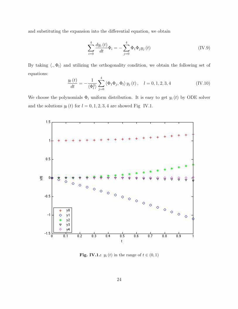
We choose the polynomials Φi uniform distribution. It is easy to get yi (t) by ODE solver
and the solutions yl (t) for l = 0, 1, 2, 3, 4 are showed Fig IV.1.
Fig. IV.1.: yi (t) in the range of t ∈ (0, 1)
24
Noting that the value of P in this example, we set as 4. To prove its correctness, we implement
a program, which computes the error measures for the mean when P is 1,2,3 and 4.
ε (t) =
∣∣∣∣y (t)− yexact (t)
yexact (t)
∣∣∣∣ (IV.11)
where
y (t) = y0 (t) , yexact (t) =et − e−t
2t(IV.12)
From Fig IV.2 , we would see that at t=1, when P=4, the error of mean of yi (t) is small
enough. There is no need to increase P to a larger number, which will lead to the complexity
of computation and longer running time consumption.
Fig. IV.2.: The error mean of of y (1) when P=1,2,3,4
25
Conclusion
In this chapter, we considered the use of polynomial-chaos based expansion techniques for
estimating the PDF of the output of a linear ODE, when the parameters in the ODE are
random variables. Polynomial-Chaos expansion is a powerful tool to estimate the PDF of
the solution of stochastic differential equations. In addition, by calculating the error of mean
square root of y (t)(at a certain time), we can find that only a small number of terms need
to be retained in the expansion to obtain good estimates of the PDF.
26
CHAPTER V
FUTURE WORKS
State and parameter estimation in bio-mechanics is a vast research topic and the research
presented in this thesis represents only a first step in the estimation of states and parameters
for certain problems. The following are important problems that need to be addressed in
the future.
• In Chapter III, only a linear ODE is considered. The response of the artery to forces is
typically given by the solution to a non-linear differential equation and hence non-linear
HMM have to be considered.
• Even for the ODE considered in Chapter III, the performance of the kernel-smoothing
algorithm is not very robust. Certain inconsistencies in the sequential monte carlo
approach were pointed out. One easy way to fix this problem is to use a non-sequential
version where an initial population is chosen for θs and fixed. However, such an ap-
proach would not be viable with θ changed with k. This model is really what is of
interest since for the purpose of diagnosis, one is interested in determining changes in
the elasticity in the artery as a function of length of the artery. Hence, there is a need
to design robust estimation techniques that work for a variety of models of change of
θk with k.
• Even though Chapter IV shows that the PDF of the output of the ODE can be found,
our interest is in using polynomial chaos expansion based methods for parameter es-
timation. We still need to develop a Bayesian inference technique based on PC for
determining the posterior density of the parameters of the ODE/HMM. Then, the ad-
vantages and disadvantages of MCMC and polynomial chaos methods for parameter
estimation problems should be compared.
27
REFERENCES
[1] D.J.C. MacKay, Information Theory, Inference and Learning Algorithms, CambridgeUniversity Press, 2003.
[2] L. R. Rabiner, B. H. Juang. An Introduction to Hidden Markov Models. IEEE ASSPJan 1986. Web. 3 Oct. 2013
[3] A. O’Hagan(2013). Polynomial Chaos: A Tutorial and Critique from a Statistician’sPerspective. Submitted to SIAM/ASA Journal of Uncertainty Quantification.
[4] Moon, Todd K, and Wynn C. Stirling. Mathematical Methods and Algorithms for SignalProcessing. Upper Saddle River, NJ: Prentice Hall, 2000. Print.
[5] M.S. Arulampalam, S. Maskell, A Tutorial on Particle Filters for Online Nonlinear/Non-Gaussian Bayesian Tracking, IEEE Transactions on Signal Processing, Vol.50, No. 2, Feb2002.
[6] J. Liu and M. West, Combined parameter and state estimation in simulation-based filter-ing, in Sequential Monte Carlo Methods , A. Doucet, J.F.G de Freitas, and N.J. Gordon,Eds New York: Springer-Verlag, 2001
[7] D. Xiu and G.E. Karniadakis, The Wiener-Askey Polynomial Chaos for Stochastic Dif-ferential Equations, SIAM J. Sci. Comput., 24(2), 619-644 (2002)