NONLINEAR APPLICATIONS OF MARKOV CHAIN MONTE CARLO

NONLINEAR APPLICATIONSOF MARKOV CHAIN MONTE CARLO

by

Gregois Lee, B.Sc.(ANU), B.Sc.Hons(UTas)

Submitted in fulfilment of the requirementsfor the Degree of Doctor of Philosophy

Department of MathematicsUniversity of Tasmania

2010

I declare that this thesis contains no material which has been acceptedfor a degree or diploma by the University or any other institution, exceptby way of background information and duly acknowledged in the thesis,and that, to the best of my knowledge and belief, this thesis containsno material previously published or written by another person, exceptwhere due acknowledgement is made in the text of the thesis.

Signed:Gregois Lee

Date:

This thesis may be made available for loan and limited copying in ac-cordance with the Copyright Act 1968

Signed:Gregois Lee

Date:

ACKNOWLEDGEMENTS

To Simon Wotherspoon for making this probable.

TABLE OF CONTENTS

TABLE OF CONTENTS i

LIST OF TABLES v

LIST OF FIGURES vii

1 Introduction 1

1.1 Statistics and Computing . . . . . . . . . . . . . . . . . . . . . . . . 1

1.2 Structure of the Thesis . . . . . . . . . . . . . . . . . . . . . . . . . . 2

1.2.1 Chapter Outlines . . . . . . . . . . . . . . . . . . . . . . . . . 3

1.2.2 R Source Code . . . . . . . . . . . . . . . . . . . . . . . . . . 4

2 Bayesian Analysis 6

2.1 Historical Context . . . . . . . . . . . . . . . . . . . . . . . . . . . . 6

2.2 Introduction . . . . . . . . . . . . . . . . . . . . . . . . . . . . . . . . 7

2.3 Bayes’ Theorem . . . . . . . . . . . . . . . . . . . . . . . . . . . . . . 8

2.4 The Prior Distribution . . . . . . . . . . . . . . . . . . . . . . . . . . 9

2.4.1 Prior Propriety . . . . . . . . . . . . . . . . . . . . . . . . . . 10

2.4.2 Non-informative Priors . . . . . . . . . . . . . . . . . . . . . . 10

2.4.3 Vague Priors . . . . . . . . . . . . . . . . . . . . . . . . . . . 11

2.4.4 Conjugate Priors . . . . . . . . . . . . . . . . . . . . . . . . . 12

2.5 The Posterior Distribution . . . . . . . . . . . . . . . . . . . . . . . . 13

2.5.1 Estimation . . . . . . . . . . . . . . . . . . . . . . . . . . . . 13

2.5.2 Inference . . . . . . . . . . . . . . . . . . . . . . . . . . . . . 13

2.5.3 Visualisation . . . . . . . . . . . . . . . . . . . . . . . . . . . 14

2.5.4 Reporting Results . . . . . . . . . . . . . . . . . . . . . . . . 14

2.6 Conclusion . . . . . . . . . . . . . . . . . . . . . . . . . . . . . . . . 16i

TABLE OF CONTENTS ii

3 Bayesian Computation 18

3.1 Introduction . . . . . . . . . . . . . . . . . . . . . . . . . . . . . . . . 18

3.2 Markov Chain Monte Carlo . . . . . . . . . . . . . . . . . . . . . . . 19

3.3 Gibbs Sampling . . . . . . . . . . . . . . . . . . . . . . . . . . . . . . 19

3.4 Metropolis-Hastings Sampling . . . . . . . . . . . . . . . . . . . . . . 20

3.5 Diagnosing Convergence . . . . . . . . . . . . . . . . . . . . . . . . . 22

3.5.1 Gelman and Rubin’s R . . . . . . . . . . . . . . . . . . . . . 22

3.5.2 Discussion . . . . . . . . . . . . . . . . . . . . . . . . . . . . . 24

3.5.3 Mixing . . . . . . . . . . . . . . . . . . . . . . . . . . . . . . . 24

3.6 Conclusion . . . . . . . . . . . . . . . . . . . . . . . . . . . . . . . . 26

4 Nonlinear Regression Models 27

4.1 Introduction . . . . . . . . . . . . . . . . . . . . . . . . . . . . . . . . 27

4.2 Linear Regression Models . . . . . . . . . . . . . . . . . . . . . . . . 28

4.3 Nonlinear Regression Models . . . . . . . . . . . . . . . . . . . . . . 29

4.4 Nonlinear Regression using MCMC . . . . . . . . . . . . . . . . . . . 30

4.4.1 Example: Biochemical Oxygen Demand . . . . . . . . . . . . 31

4.5 Growth Curve Models using MCMC . . . . . . . . . . . . . . . . . . 37

4.5.1 Ratkowsky’s Regression Strategy . . . . . . . . . . . . . . . . 37

4.5.2 Model Functions and Data . . . . . . . . . . . . . . . . . . . 37

4.5.3 Three Parameter Models . . . . . . . . . . . . . . . . . . . . 40

4.5.4 Four Parameter Models . . . . . . . . . . . . . . . . . . . . . 47

4.5.5 Troubleshooting . . . . . . . . . . . . . . . . . . . . . . . . . 54

4.6 Discussion . . . . . . . . . . . . . . . . . . . . . . . . . . . . . . . . . 60

4.6.1 Back Transformation . . . . . . . . . . . . . . . . . . . . . . . 60

4.6.2 Posterior Curvature . . . . . . . . . . . . . . . . . . . . . . . 61

4.7 Conclusion . . . . . . . . . . . . . . . . . . . . . . . . . . . . . . . . 63

5 Response Transformations 65

5.1 Introduction . . . . . . . . . . . . . . . . . . . . . . . . . . . . . . . . 65

5.2 The Method . . . . . . . . . . . . . . . . . . . . . . . . . . . . . . . . 66

5.2.1 Discussion . . . . . . . . . . . . . . . . . . . . . . . . . . . . . 67

5.3 Example: Toxic Agents . . . . . . . . . . . . . . . . . . . . . . . . . 68

5.3.1 Model Fitting . . . . . . . . . . . . . . . . . . . . . . . . . . . 69

TABLE OF CONTENTS iii

5.3.2 Model Checking . . . . . . . . . . . . . . . . . . . . . . . . . 70

5.3.3 Box-Cox Transformation . . . . . . . . . . . . . . . . . . . . . 70

5.3.4 Evaluating the Transformed Model . . . . . . . . . . . . . . . 72

5.3.5 MCMC Transformation . . . . . . . . . . . . . . . . . . . . . 72

5.4 Conclusion . . . . . . . . . . . . . . . . . . . . . . . . . . . . . . . . 78

6 Monotonic Additive Models 79

6.1 Introduction . . . . . . . . . . . . . . . . . . . . . . . . . . . . . . . . 79

6.2 Method Details . . . . . . . . . . . . . . . . . . . . . . . . . . . . . . 80

6.3 Example: Simulated Data . . . . . . . . . . . . . . . . . . . . . . . . 81

6.3.1 Data Generation . . . . . . . . . . . . . . . . . . . . . . . . . 81

6.3.2 Model Fitting . . . . . . . . . . . . . . . . . . . . . . . . . . . 82

6.3.3 Results . . . . . . . . . . . . . . . . . . . . . . . . . . . . . . 82

6.4 Example: Black Cherry Trees . . . . . . . . . . . . . . . . . . . . . . 85

6.4.1 Model Fitting . . . . . . . . . . . . . . . . . . . . . . . . . . . 85

6.4.2 Results . . . . . . . . . . . . . . . . . . . . . . . . . . . . . . 88

6.5 Example: US Temperature Data . . . . . . . . . . . . . . . . . . . . 92

6.5.1 Model Fitting . . . . . . . . . . . . . . . . . . . . . . . . . . . 93

6.5.2 Results . . . . . . . . . . . . . . . . . . . . . . . . . . . . . . 93

6.6 Conclusion . . . . . . . . . . . . . . . . . . . . . . . . . . . . . . . . 95

7 Estimating Correlations 97

7.1 Introduction . . . . . . . . . . . . . . . . . . . . . . . . . . . . . . . . 97

7.2 Sampling Strategy . . . . . . . . . . . . . . . . . . . . . . . . . . . . 98

7.2.1 Introduction . . . . . . . . . . . . . . . . . . . . . . . . . . . 98

7.2.2 Implications of the Positive Definite Constraint . . . . . . . . 98

7.2.3 Determining the Sampling Interval . . . . . . . . . . . . . . . 99

7.2.4 Refactoring the Trace . . . . . . . . . . . . . . . . . . . . . . 100

7.2.5 Rejection Sampling . . . . . . . . . . . . . . . . . . . . . . . . 100

7.3 Implementation . . . . . . . . . . . . . . . . . . . . . . . . . . . . . . 101

7.3.1 Example: Estimating a Single Variance Matrix Element . . . 101

7.3.2 Rejection Rates . . . . . . . . . . . . . . . . . . . . . . . . . . 104

7.3.3 The Griddy-Gibbs Sampler . . . . . . . . . . . . . . . . . . . 104

7.3.4 Example: Estimating Multiple Matrix Entries . . . . . . . . . 107

TABLE OF CONTENTS iv

7.4 Conclusion . . . . . . . . . . . . . . . . . . . . . . . . . . . . . . . . 110

8 Conclusion 111

8.1 Synopsis . . . . . . . . . . . . . . . . . . . . . . . . . . . . . . . . . . 111

8.2 Thesis Summary . . . . . . . . . . . . . . . . . . . . . . . . . . . . . 112

8.3 Further Research . . . . . . . . . . . . . . . . . . . . . . . . . . . . . 114

8.3.1 Nonlinear Regression Models . . . . . . . . . . . . . . . . . . 114

8.3.2 Monotonic Additive Models . . . . . . . . . . . . . . . . . . . 114

8.4 Concluding Remarks . . . . . . . . . . . . . . . . . . . . . . . . . . . 115

A Source Code 116

A.1 Chapter 4 . . . . . . . . . . . . . . . . . . . . . . . . . . . . . . . . . 116

A.2 Chapter 5 . . . . . . . . . . . . . . . . . . . . . . . . . . . . . . . . . 125

A.3 Chapter 6 . . . . . . . . . . . . . . . . . . . . . . . . . . . . . . . . . 128

A.4 Chapter 7 . . . . . . . . . . . . . . . . . . . . . . . . . . . . . . . . . 130

BIBLIOGRAPHY 144

LIST OF TABLES

4.1 Biochemical Oxygen Demand Data . . . . . . . . . . . . . . . . . . . 31

4.2 Summary Statistics: BOD Data Model. . . . . . . . . . . . . . . . . 35

4.3 Bean Data . . . . . . . . . . . . . . . . . . . . . . . . . . . . . . . . . 38

4.4 Cucumber Data . . . . . . . . . . . . . . . . . . . . . . . . . . . . . . 38

4.5 Onion Data . . . . . . . . . . . . . . . . . . . . . . . . . . . . . . . . 39

4.6 Pasture Data . . . . . . . . . . . . . . . . . . . . . . . . . . . . . . . 39

4.7 Summary Statistics: Gompertz Models. . . . . . . . . . . . . . . . . 41

4.8 Summary Statistics: Logistic Models. . . . . . . . . . . . . . . . . . . 42

4.9 Summary Statistics: Morgan-Mercer-Flodin Models. . . . . . . . . . 48

4.10 Summary Statistics: Richards Models. . . . . . . . . . . . . . . . . . 50

4.11 Summary Statistics: Weibull-type Models. . . . . . . . . . . . . . . . 52

4.12 Curvature Component Estimates. . . . . . . . . . . . . . . . . . . . . 54

4.13 Summary Statistics: Reparameterised MMF Models. . . . . . . . . . 56

4.14 Summary Statistics: Reparameterised Weibull Models. . . . . . . . . 59

4.15 Summary Statistics: Back-Transformed Weibull-Pasture Data. . . . 61

5.1 Toxic Agent Data, (Box and Cox, 1964) . . . . . . . . . . . . . . . . 68

5.2 ANOVA: Poison Model . . . . . . . . . . . . . . . . . . . . . . . . . . 69

5.3 ANOVA: Reciprocal Transformed Poison Model . . . . . . . . . . . . 72

5.4 ANOVA: MCMC Transformed Poison Model . . . . . . . . . . . . . 74

5.5 Parameter Estimates: Transformed Poison Model (5.11) . . . . . . . 76

6.1 Parameter Estimates: Monotonic Additive Model (6.8) . . . . . . . . 83

6.2 Cherry Tree Data . . . . . . . . . . . . . . . . . . . . . . . . . . . . . 86

6.3 Parameter Estimates: Trees Model (6.9) . . . . . . . . . . . . . . . . 88

6.4 Parameter Estimates: US Temperature Model . . . . . . . . . . . . . 94

v

LIST OF TABLES vi

7.1 Bi-Gamma Sampling Distribution Summary . . . . . . . . . . . . . . 103

7.2 Griddy-Gibbs Sampling Distribution Summary . . . . . . . . . . . . 108

7.3 Bi-Gamma Sampling Distribution Summary x = vij , n = 10 . . . . . 109

7.4 Bi-Gamma Sampling Distribution Summary x = vij , n = 100 . . . . 110

LIST OF FIGURES

2.1 Data Driven Posterior. . . . . . . . . . . . . . . . . . . . . . . . . . . 12

2.2 Disjoint Highest Posterior Density Interval. . . . . . . . . . . . . . . 15

3.1 Metropolis Proposal Tuning. . . . . . . . . . . . . . . . . . . . . . . . 25

4.1 BOD Data with Initial Parameter Value Fit. . . . . . . . . . . . . . 32

4.2 Adaptive MCMC Trace: BOD Model. . . . . . . . . . . . . . . . . . 33

4.3 MCMC Posterior Sample Trace: BOD Model. . . . . . . . . . . . . . 34

4.4 Fitted BOD Model. . . . . . . . . . . . . . . . . . . . . . . . . . . . . 36

4.5 Pairwise Marginal Scatterplots: BOD Model. . . . . . . . . . . . . . 36

4.6 Fitted Gompertz-Cucumber Model. . . . . . . . . . . . . . . . . . . . 40

4.7 Fitted Gompertz-Onion Model. . . . . . . . . . . . . . . . . . . . . . 43

4.8 Fitted Logistic-Cucumber Model. . . . . . . . . . . . . . . . . . . . . 44

4.9 Pairwise Marginal Scatterplots: Cucumber-Gompertz-Cucumber Model. 45

4.10 MCMC Posterior Sample Trace: Gompertz-Cucumber Model. . . . . 45

4.11 (Median) Fitted Gompertz-Cucumber Model. . . . . . . . . . . . . . 46

4.12 Fitted MMF-Cucumber Model. . . . . . . . . . . . . . . . . . . . . . 47

4.13 Fitted MMF-Onion Model. . . . . . . . . . . . . . . . . . . . . . . . 49

4.14 Fitted Richards-Cucumber Model. . . . . . . . . . . . . . . . . . . . 51

4.15 Pairwise Marginal Scatterplots: Richards-Cucumber Model. . . . . . 53

4.16 Fitted Weibull-Pasture Model. . . . . . . . . . . . . . . . . . . . . . 53

4.17 Fitted Reparameterised MMF-Onion Model. . . . . . . . . . . . . . . 57

4.18 Fitted Simulated Richards-Cucumber Model. . . . . . . . . . . . . . 58

4.19 Fitted Reparameterised Weibull-Pasture Model. . . . . . . . . . . . . 60

4.20 Marginal Scatterplots: MMF-Onion Model. . . . . . . . . . . . . . . 62

4.21 Marginal Scatterplots: Reparameterised MMF-Onion Model. . . . . 63

vii

LIST OF FIGURES viii

5.1 Survival Time by Experimental Factor . . . . . . . . . . . . . . . . . 69

5.2 Diagnostic Plots: Poison Model . . . . . . . . . . . . . . . . . . . . . 70

5.3 Profile Log Likelihood, Box-Cox Transformation . . . . . . . . . . . 71

5.4 Diagnostic Plots: Transformed Poison Model . . . . . . . . . . . . . 73

5.5 Transformed Survival Time by Experimental Factor . . . . . . . . . 74

5.6 MCMC Estimated Response Transformation . . . . . . . . . . . . . . 75


5.8 Residuals vs Fitted Values: MCMC Transformed Model . . . . . . . 77


6.1 Simulated Data against Covariate x1 . . . . . . . . . . . . . . . . . . 82

6.2 Simulated Data against Covariate x2 . . . . . . . . . . . . . . . . . . 83

6.3 Estimated Monotonic Function f1 . . . . . . . . . . . . . . . . . . . 84

6.4 Estimated Monotonic Function f2 . . . . . . . . . . . . . . . . . . . 85

6.5 Black Cherry Trees: Timber Volume by Tree Girth . . . . . . . . . . 87

6.6 Black Cherry Trees: Timber Volume by Tree Height . . . . . . . . . 87

6.7 Estimated Transformation: Tree Girth . . . . . . . . . . . . . . . . . 89

6.8 Estimated Transformation: Tree Height . . . . . . . . . . . . . . . . 90

6.9 Fitted Mean: Timber Volume by Tree Girth . . . . . . . . . . . . . . 90

6.10 Actual Timber Volume by Fitted Volume . . . . . . . . . . . . . . . 91

6.11 Pairwise Scatterplots: US Temperature Data . . . . . . . . . . . . . 92

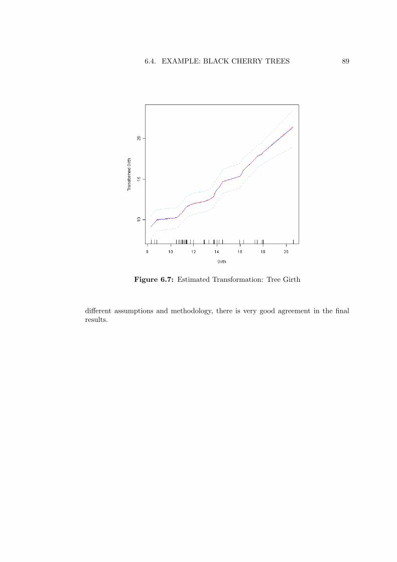
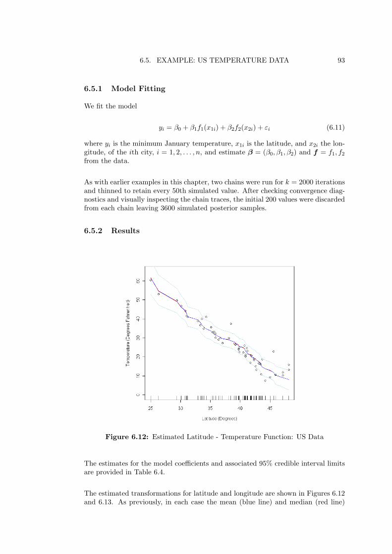
6.12 Estimated Latitude - Temperature Function: US Data . . . . . . . . 93

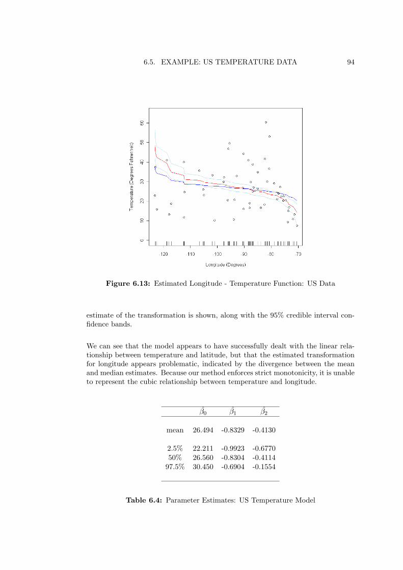
6.13 Estimated Longitude - Temperature Function: US Data . . . . . . . 94

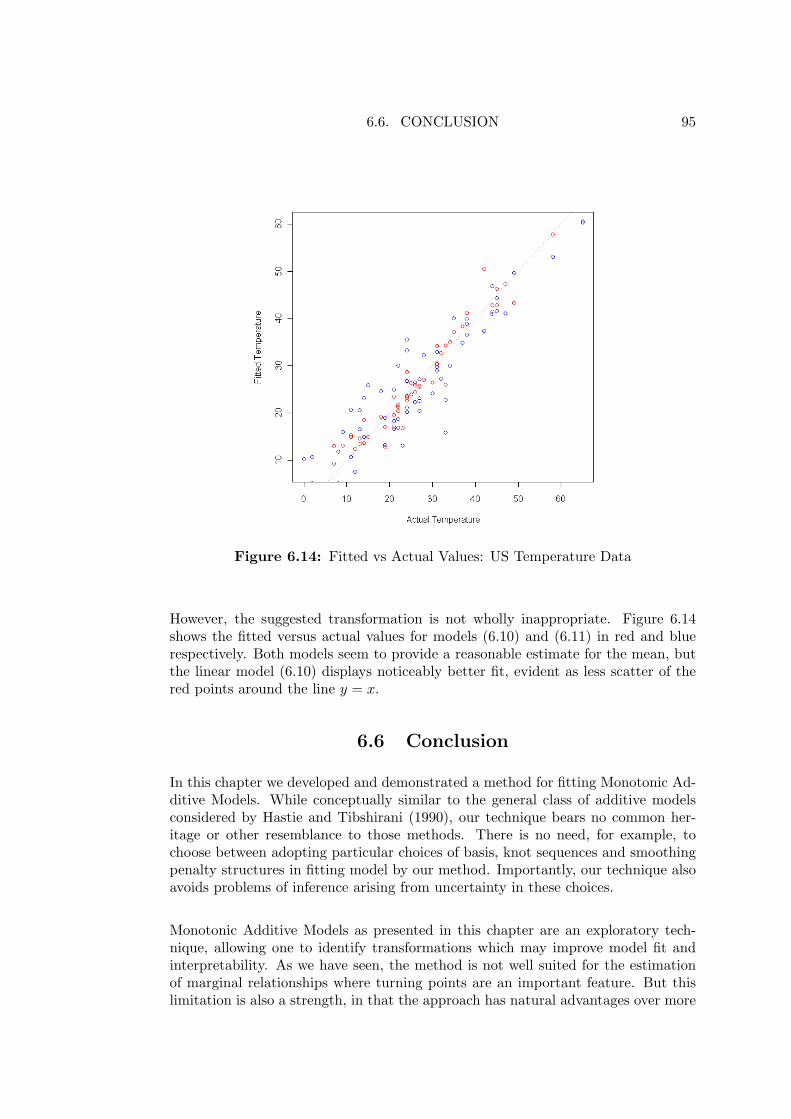
6.14 Fitted vs Actual Values: US Temperature Data . . . . . . . . . . . . 95

7.1 Bi-Gamma Sampling Distribution for x = v12 . . . . . . . . . . . . . 103

7.2 Evaluating the Posterior on a Grid . . . . . . . . . . . . . . . . . . . 105

7.3 Approximating the Cumulative Distribution Function . . . . . . . . 106

7.4 Transforming a Uniform Random Deviate via Griddy Gibbs . . . . . 107

7.5 Griddy Gibbs Sampling Distribution for x = v12 . . . . . . . . . . . 108

Chapter 1

Introduction

1.1 Statistics and Computing

In the early 20th century data analysis was constrained by computability. Cal-culations were performed by hand, providing real practical limits on the types ofproblems which were tractable. Salsburg (2002) provides a calculation showing thatat least 8 months of 12-hour days would have been required for R. A. Fisher to haveproduced the tables in his “Studies in Crop Variation I” (Fisher, 1921) with themechanical means at his disposal. It is hardly surprising that the emphasis duringthis period remained on linear models – problems soluble by ordinary least squares,with the tools at hand.

It was not until the 1960s that nonlinear regression began to appear regularly in theliterature, and no accident that this eventuates concurrently with the appearanceof machines to automate iterative calculations. The heavier computational burdenhad previously been insurmountable. But even after the advent of early computers,great emphasis was placed on the development of algorithms which could make effi-cient use of limited hardware resources – processors were slow and memory limited.Research into algorithms became synonymous with efficiency, and the attendantO-notation. The Fast Fourier Transform of Cooley and Tukey (1965) provides thearchetypal example of the era. The explicit reference to speed in the title under-scores the imperative.

In the early 21st century, the situation has improved markedly. Computing poweris cheap and relatively abundant, and software is designed with re-use of objectsand systems integration in mind. There has been a co-evolution of research intomodelling methods. Modelling frameworks have diversified, and are now capable ofrepresenting a much broader range of observable phenomena. Informed by Tukey’sobservation “Far better an approximate answer to the right question, ... than anexact answer to the wrong question” (Tukey, 1962), we build models which moreaccurately reflect our understanding of reality. Increasingly, we are asking the rightquestions.

1

1.2. STRUCTURE OF THE THESIS 2

Indeed, since the 1970s there has been rapid development in methods which ex-tend the general linear model, stimulated by the development of Generalized LinearModels (GLMs) (McCullagh and Nelder, 1989). These allow response residuals tobe modelled using alternatives to the Gaussian distribution and conditional expec-tations to be related to covariates via a link function η(θ), rather than a directlinear relationship. The general linear model can then be seen as a GLM with anidentity link function and a normally distributed response. The principal appeal ofthe framework is that the adoption of the exponential family as the basis guaranteesthe likelihood to be log-concave and unimodal so that estimation is straightforward.The adoption of GLMs has greatly extended the realm of linear models and vastlyenhanced the scope of linear statistical modelling applications. What remains con-spicuously absent is concurrent progress of a similar order in pursuit of nonlinearmodels, where the properties of the solution surface are more complex.

The adoption of Markov Chain Monte Carlo (MCMC) techniques by the statisticalcommunity represents a significant new chapter in stochastic modelling. MCMCmethods provide a flexible and powerful base from which realistic stochastic modelscan be built. They are particularly important because models developed in thisframework need not have analytical tractability. Provided that the relationshipsbetween the component parts are specified, samples can be obtained from the den-sity of the resulting model, allowing estimation and inference from non-standarddistributions. This is an enormously empowering development. Most importantly,it promotes the construction of more realistic models. Data no longer need be forcedinto overly simplistic models just because they are the only soluble forms. Modelscan now be developed to fit available data.

The development of MCMC tools have fundamentally altered the way that statisti-cians go about their business. But it is not merely statisticians who benefit. Greateraccessibility of realistic modelling methods has led to statistical modelling taking afirm hold in primary research across a wide range of applied disciplines. The ex-change of purely deterministic models in favour of more realistic stochastic modelsrepresents a paradigm shift in the foundation of science.

1.2 Structure of the Thesis

This thesis considers the application of Markov Chain Monte Carlo (MCMC) meth-ods to problems which extend the general linear model in various nonlinear ways.The framework in which these applications are developed is exclusively Bayesian,though the the methods themselves are equally applicable, if perhaps less commonlyused, in a likelihood context. Geyer (1995) and Diebolt and Ip (1995), and the ref-erences therein, provide details of non-Bayesian applications of MCMC.


1.2.1 Chapter Outlines

Chapter 2 provides an overview of Bayesian methodology and nomenclature. Webegin by establishing the historical context of the development of Bayesian methodsand the recent rise in popularity of their use. This is followed by the introduction ofBayes’ theorem and an example illustrating its use. The prior distribution is thenexamined in greater detail, with a discussion of relative states of prior information,the use of conjugate priors, and further development of the example. We then turnto a discussion of the posterior distribution, its role in Bayesian inference and esti-mation, and how results are reported and interpreted.

Chapter 3 provides an overview of Markov Chain Monte Carlo (MCMC) methods.In particular the Gibbs Sampler and the Metropolis-Hastings algorithm are intro-duced. These computational techniques underpin the implementation of all themethods explored in later chapters. The concept of partitioning the posterior intomanageable parts is fundamental to implementing an appropriate sampling scheme.In cases where this can be achieved with the full conditional distribution availablein an analytical form, Gibbs Sampling provides a very efficient mechanism for pro-ducing posterior samples. In cases where a closed-form solution is not available, aMetropolis-Hastings sampling scheme can be implemented. This involves generatingsamples from a proposal distribution, and subjecting proposed points to a rejectionfilter such that candidates are accepted with probability matching that of the targetposterior distribution. The details of how this can be achieved are described beforemoving on to a discussion of convergence issues in MCMC. Gelman and Rubin’spotential scale reduction factor R is described. Finally, we give a brief account ofvisual inspection of the MCMC chain trace and its use as a qualitative aid in as-sessing whether the support of the posterior has been appropriately sampled.

Having established the conceptual and computational framework for the thesis, weturn to application of these tools.

Chapter 4 demonstrates the use of Bayesian MCMC in the nonlinear regressioncontext. This allows the model mean to take the form of a parametric nonlinearfunction. We begin by reviewing Least Squares parameter estimation in nonlinearmodels, and propose an MCMC alternative. A simple example is developed to il-lustrate the use of the MCMC method. Next, we undertake a detailed evaluation ofthe method’s performance in the context of growth curve models. The main focusof the chapter is a comparative analysis with the Least Squares results provided byRatkowsky (1983). We show that the MCMC method offers results comparable tothose obtained under Least Squares across a range of nonlinear regression problems,and offers several significant advantages.

Chapter 5 describes a method for transforming the response using Gibbs Sampling.That is, we consider nonlinear transformations of the response such that the cri-teria required by the general linear model are met by the transformed variable,and modelling may proceed under the general linear framework. The method si-


multaneously estimates the response transformation along with parameters to fit anassumed linear model. This approach is of particular interest because it incorporatesuncertainty in the choice of transformation into the modelling process, in contrastwith many other methods of transformation currently in use. We demonstrate thesuccessful application of the method by reconsidering an example put forward byBox and Cox (1964), and provide a comparative analysis with the results suggestedby their method.

Chapter 6 extends the method introduced in the previous chapter to consider caseswhere the response can be represented as the sum of monotonic functions of covari-ates: Monotonic Additive Models. This is another example of relaxing linearity asthe assumed form of the conditional mean response, but here the relationship of theresponse to each covariate is nonparametric in form.

In principle, our approach is similar to that of nonparametric additive models (Hastieand Tibshirani, 1990), in that we seek to find a series of nonparametric functionsrepresenting the relationship of each covariate to the response and combine these inan additive framework. Yet the mechanism by which we achieve this end is quitenovel, and bears no relationship to the class of additive models considered by Hastieand Tibshirani (1990) beyond its conceptual structure. We develop a series of ex-amples using simulated and real data to critically evaluate the performance of themethod.

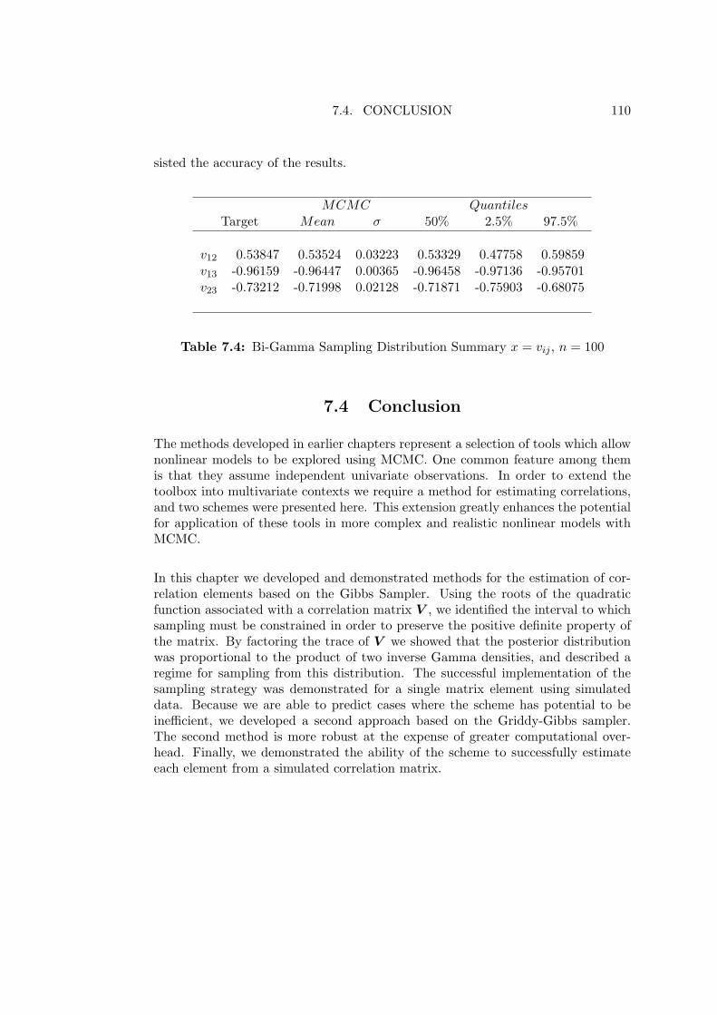
To extend the techniques of earlier chapters for use in multivariate or mixed-effectsmodels, a method for modelling the correlation structure between estimands is re-quired. In Chapter 7 we develop techniques for estimating correlations using variantsof the Gibbs sampler. The principal method uses a rejection sampling strategy basedupon carefully selected Gamma distributions. Another method is provided for usein cases where this approach can be demonstrated to operate with low efficiency.Both methods are tested against simulated data to illustrate their relative merits.A detailed account of the practical issues involved in the successful implementationof the techniques is provided.

Finally, Chapter 8 summarises the results presented in the thesis, offers concludingremarks, and identifies areas where the techniques developed in the thesis can beextended in future research. We propose enhancements to individual methods andapplications where they may be applied in concert.

1.2.2 R Source Code

Many of the examples in the thesis could be implemented using variants of the BUGS(Bayesian inference Using Gibbs Sampling) environment (Lunn et al., 2000; Thomaset al., 2006; Plummer, 2003). However, examples which feature strong correlationbetween parameters mix poorly under the Gibbs sampler, and require very long runtimes to produce reasonable estimates. In particular, Chapters 4 & 7 investigateproblems where it would be unrealistic to ignore cases of highly correlated estimates.


Rather than distract the reader by chopping and changing between developmentenvironments we elected to conduct all analyses and development of source codein the preparation of this thesis in the R statistical environment (R DevelopmentCore Team, 2009). The source code used in producing results presented herein isprovided in Appendix A.

Chapter 2

Bayesian Analysis

2.1 Historical Context

Early Development

In 1763 the Philosophical transactions of the Royal Society of London published aposthumous article by the reverend Thomas Bayes, with the title Essay TowardsSolving a Problem in the Doctrine of Chances (reprinted in Biometrika using no-tation familiar to the modern reader as Barnard and Bayes, 1958). In essence, thearticle presented a model for inductive logic, inverse probability, using observationaldata to enhance an observer’s prior beliefs in the probability of an event occurring.The theory was accepted at the time of it’s publication, and further developed intowhat can be recognised as the foundations of modern probability theory by the em-inent French mathematician Pierre-Simon Laplace in the late 18th and early 19thcentury (Stigler, 1990; Hald, 1998; Dale, 1999).

Bayes’ mathematics remain unchallenged. But the logician George Boole (1854,republished as Boole, 2008) is attributed with being the first to call into questionthe philosophical validity of allowing subjective criteria to enter into the probabil-ity calculus, and sparking a controversy that troubled statisticians for over a century.

The 20th Century

In the context of the ensuing debate, R. A. Fisher was at pains to justify the foun-dations of the emerging discipline of statistics in opposition to Bayesian principles(Fisher, 1922, 1925b). The result was what is today recognised as a frequentistapproach; that is, a system of statistical procedures which are founded upon, andjustified relative to, consideration of all samples which could conceivably arise in agiven context. Despite Fisher’s insight that for statistics to be useful, it must be ca-pable of deriving results from sample sizes that researchers can realistically achieve(see, for example, Fisher, 1925a, 1935, re-issued as Fisher et al. (1990)), it is commonfor frequentist theory to be justified asymptotically – in light of infinite sample sizes.

6

2.2. INTRODUCTION 7

Harold Jeffreys, a contemporary of Fisher, was interested in establishing a consis-tent probabilistic basis for the scientific method. His outlook was Bayesian, andhis scientific output prodigious. A succinct summary of Jeffreys’ contributions tostatistics and how these relate to the work of Fisher and Bayes is given in Jeffreys(1974). Jeffreys’ (ultimately) influential works Scientific Inference (1931, re-issuedas Jeffreys, 2007) and Theory of Probability (1961, re-issued as Jeffreys, 1998) wereinstrumental in re-kindling Bayesian methods in statistics in the latter half of the20th century. Other important contributions following on from the work of Jeffreyswere made by L. J. Savage (Savage, 1954), Dennis Lindley (particularly Lindley,1965a,b), Bruno de Finetti (de Finetti, 1974, 1975), and Edwin Jaynes (Jaynes,2003), among others. Press (2003) contains biographical sketches of these authorsand synopses of their work.

A Recent Renaissance

In recent years the ubiquity of unprecedented desktop computing power has en-abled Bayesian methods to flourish, both in the statistical community and outsideit. Berger (2000) describes the increase in Bayesian activity at the turn of themillennium, as indexed by the number of published research articles, the numberof books, and the extensive number of Bayesian applications appearing in applieddisciplines. This trend has continued to date. In addition to mainstream statisticaltomes (prominent examples include Gelman et al., 2003; Carlin and Louis, 2008),texts clearly targeted at beginning undergraduate students are emerging (see, for ex-ample, Bolstad, 2007), with the implication that in some quarters at least, Bayesianmethods are being incorporated into students’ foundation in statistics. Significantly,practitioners in applied disciplines have embraced the Bayesian approach, with textscommonly appearing, for example, in fields such as clinical studies (Spiegelhalteret al., 2004; Broemeling, 2007; Grobbee and Hoes, 2008), ecology (McCarthy, 2007;Bolker, 2008; Royle and Dorazio, 2008; King et al., 2009), economics (Lancaster,2004; Geweke, 2005; Greenberg, 2007; Koop et al., 2007), epidemiology (Banerjeeet al., 2003; Moye, 2007; Lawson, 2008), finance (Singpurwalla, 2006; Scherer andMartin, 2007; Rachev et al., 2008), and the social sciences (Gelman and Hill, 2007;Gill, 2007; Jackman, 2009). Clearly, Bayesian methods have come of age.

2.2 Introduction

Bayesian analysis differs from its frequentist counterpart in two important respects:

i) from the Bayesian viewpoint all estimands are random variables with an as-sociated probability distribution, and

ii) Bayesian analysis provides a formal mechanism for admitting subjective infor-mation into the model structure.

2.3. BAYES’ THEOREM 8

The implications of these attributes are profound. Bayesian analysis is fundamen-tally different from frequentist analysis, both in terms of mechanics and interpreta-tion. This chapter will outline these differences and their implications.

2.3 Bayes’ Theorem

Given a vector of observations y whose probability distribution p(y|θ) is conditionalupon the parameter vector θ, which itself has probability distribution p(θ), then

p(y|θ)p(θ) = p(θ|y)p(y), (2.1)

where the notation p(a|b) denotes the probability of an event a occurring subject tothe condition that b occurs. As we will generally be interested in the distributionof the parameter vector, given the observed data, we write Bayes’ Theorem as

p(θ|y) =p(y|θ)p(θ)

p(y), (2.2)

where p(y) is a normalisation constant, ensuring that the expression on the righthand side of (2.2) integrates, or sums, to unity.

From (2.2) we see that the distribution of the parameters θ given the data y is theproduct of two terms: the conditional probability of observing the data y given theparameters θ, and the probability distribution of those parameters, p(θ). Viewed asa function of θ, the first term is the likelihood function for the parameters θ giventhe observations y. The second term is referred to as the prior distribution of θ, toreflect the idea that the information contained in this term is independent from, andcan be considered as arising prior to, observation of the data. Finally, the productp(θ|y) is termed the posterior distribution, reflecting the idea that it represents thestate of knowledge resulting from the modification of prior knowledge regarding θby the information contained in the observations y.

Example

Suppose we have a single observation y, the realisation of a normally distributedrandom variable Y ∼ N (µ, σ2) with known variance σ2. The likelihood function forθ = µ is then

l(θ; y) = p(y|θ) = N (y|µ, σ2) ≡ 1σ√

2πe−

(y−µ)2

2σ2 ,

where N (y|µ, σ2) indicates the likelihood of observing the data y conditional on thevalues of the parameters µ and σ2. As the likelihood is a function of the parame-ters, Maximum Likelihood methods seek to estimate θ such that it maximises the

2.4. THE PRIOR DISTRIBUTION 9

probability of observing the data y.

Next we require a distribution to represent our prior beliefs regarding possible valuesfor the value of θ. If we consider that a reasonable choice is a normal distributionwith mean η and variance φ, we may write p(θ) = N (µ|λ), where λ = (η, φ), arehyper-parameters in the model. That is, they provide structure to the model byinforming how model parameters are to be constrained. It is now apparent thatwe are considering a hierarchy of model parameters: here µ is constrained by thechoice of λ. It is possible to estimate all elements of the parameter hierarchy fromthe data (see, for example, Gelman et al., 2003), but for the sake of exposition wedo not consider that case here. With the likelihood and prior in place we are nowready to apply Bayes’ Theorem

p(θ|y) =N (y|µ, σ2) N (µ|λ)

p(y)∝ N (y|µ, σ2) N (µ|η, φ2)

= N(µ∣∣∣ φ2

σ2 + φ2y +

σ2

σ2 + φ2η,

σ2φ2

σ2 + φ2

).

(2.3)

That is, the distribution of µ given the observation y is also a normal distribu-tion, with the mean and variance shown in (2.3). The expected value E(θ|y) is theweighted average of the observation value y and the prior mean η, with weightsdependent on the respective levels of uncertainty associated with the prior and thelikelihood.

The variance associated with θ is constructed in terms of its reciprocal, the precisionτ = 1

σ2 , which is more convenient to work with in a Bayesian context and offers anintuitive interpretation here: the posterior precision is the sum of the precisionsfrom the likelihood and the prior, 1

σ2 + 1φ2 .

2.4 The Prior Distribution

The prior distribution provides the formal mechanism through which subjective in-formation can be included in the modelling process. It allows freedom to nominatea distribution of values associated with the parameter vector θ, consistent with therange of values that θ is believed likely to assume.

In the example of §2.3 we saw that the expected value E(θ|y) was the precisionweighted average of the of the prior mean and the observed data, and that theweights were determined by the relative precision of these distributions. Influenceover the location of p(θ|y) was provided by the choice of the prior mean η, and thedegree to which the preference for that value was exerted was provided by the prior


precision, τ = 1φ2 .

This ability to incorporate prior information into the probability calculus in a care-fully controlled formal manner has been cited (Lindley, 1965a,b; de Finetti, 1974,1975; Berger, 2006, for example) as a major advantage of Bayesian analysis. How-ever, it is precisely this feature which has formed the focal point for contention withfrequentist stalwarts. The power to influence analytical outcomes implies a respon-sibility to understand and evaluate the implications of such choices. The remainderof this section will consider the issues associated with choosing appropriate priordistributions.

2.4.1 Prior Propriety

The prior distribution p(θ) provides a probability model of plausible values for theparameter vector θ. A fundamental property we expect of any probability functionis

∫p(θ) dθ∑p(θ)

}= 1,

regardless of whether θ is continuous or discrete. Situations arise in which we maywish to express a lack of preference for any value of θ. Yet if we try to take p(θ) tobe uniform over the entire real line, the prior

p(θ) = c > 0, −∞ < θ <∞,

is not a proper probability density since the integral

∫ ∞−∞

p(θ)dθ = c

∫ ∞−∞

dθ

does not exist for any value c. Although the result is not a probability density ina strict sense, such distributions are sometimes employed as prior distributions toexpress indifference between values of θ in some local region where the likelihoodfunction attains appreciable density. These distributions are termed improper priorsto reflect their degenerate nature. The posterior distributions which arise fromimproper priors are frequently proper probability densities, allowing some flexibilityin the specification of priors without impediment to subsequent inference.

2.4.2 Non-informative Priors

A prior distribution which does not favour any particular value of θ over any othermay be said to be “non-informative” for θ. Such distributions have the appeal thatposteriors arising from their use are free from the subjective influence of the prior.For this reason they may sometimes be used as a “reference” prior; a benchmark


against which the sensitivity of posterior outcomes for other prior distributions maybe evaluated.

Box and Tiao (1973) provide an example of non-informative priors supposing asample y ∼ N (θ, σ2), where σ is known. The likelihood for θ is

l(θ|σ, y) ∝ exp[− n

2σ2(θ − y)2], (2.4)

and under this scenario a non-informative prior is locally uniform in θ

p(θ) ∝ c. (2.5)

However, if the quantity of primary interest were instead κ = θ−1, the likelihoodbecomes

l(κ|σ, y) ∝ exp[− n

2σ2(κ−1 − y)2], (2.6)

and since

p(κ) = p(θ)∣∣∣dθdκ

∣∣∣ = p(θ)θ2 ∝ κ−2, (2.7)

the corresponding non-informative prior for κ is proportional to κ−2. In general,if a prior distribution is locally uniform for some (monotonic) function of the pa-rameter(s) of interest φ(θ), then the corresponding non-informative prior for θ isproportional to |dφ/dθ|.

2.4.3 Vague Priors

In practice we need not be overly concerned with strictly non-informative priors,provided that the prior is relatively uninformative when compared to the informationcontained in the data. The prior should include all plausible values for θ but neednot be concentrated around the true value, because information regarding θ in thedata will typically outweigh any reasonable prior probability specification.

Example (continued)

Consider an extension of the example presented in §2.3 where a sample of size nis available. Since the sample mean y is sufficient for θ, p(θ|y) = p(θ|y), and sincep(y|θ) = N (θ, σ2/n),

p(θ|y) = N(θ∣∣∣(σ2/n)µ+ φ2y

(σ2/n) + φ2,

(σ2/n)φ2

(σ2/n) + φ2

)= N

(θ∣∣∣σ2µ+ nφ2y

σ2 + nφ2,

σ2φ2

σ2 + nφ2

).

(2.8)


From (2.8) it is again clear that the posterior is a weighted average of the prior anddata values, but now it is also apparent that the relative weighting is proportionalto the number of observations n. As the number of observations increases the rel-ative influence of the prior distribution is diminished. If n is sufficiently large, theinfluence exerted by the prior distribution is overwhelmed and becomes negligible.

Figure 2.1: Data Driven Posterior.

Where the prior is relatively uninformative, n does not need to be very large. Fig-ure 2.1 shows the relative influence of the prior p(θ) ∼ N (2, 2) on the posteriordistributions resulting from simulated observational data y ∼ N (4, 1) for n = 1 andn = 6, respectively. A single observation from these data is sufficient to establishthat the mean of the posterior is considerably larger than that of the prior. With6 observations, the posterior has become focused near the true value of θ = 4 withfar greater precision.

2.4.4 Conjugate Priors

In the example of §2.3 the application of Bayes theorem using a normal prior led to aposterior which was also a normal distribution. Raiffa and Schlaifer (1961) pointedout that some priors give rise to posteriors from the same family of distributions.Formally, we may write that if P is a class of prior distributions for θ, and F is aclass of sampling distributions, then P is conjugate for F if

2.5. THE POSTERIOR DISTRIBUTION 13

p(θ|y) ∈ P for all p(.|θ) ∈ F and p(.) ∈ P. (2.9)

Of particular interest are the natural conjugate families for the prior, which havethe same functional form as the likelihood. This property then offers a very con-venient structure for performing iterative calculations with Bayes Theorem. Theconjugate prior gives rise to a posterior distribution from the same density family.Thus the posterior resulting from iteration t can be regarded as the prior during asubsequent iteration t + 1. Successive modification of the posterior by subsequentiterative application of Bayes Theorem is referred to as Bayesian learning, reflectingthe update of prior beliefs in light of the data.

2.5 The Posterior Distribution

The left-hand side of (2.2) results from combining information available in the ob-served data y, with any prior knowledge regarding the range of likely values forthe parameters, via the likelihood function l(θ;y) = p(y|θ) and prior distributionp(θ), respectively. The distribution p(θ|y) is commonly referred to as the posteriordistribution for θ, because it expresses the state of knowledge regarding parametervalues after modifying prior beliefs by the information available in the observations.

2.5.1 Estimation

In cases where the posterior can be written in closed analytical form, summariesmay be obtained directly from the properties of the posterior distribution (see, forexample, Gelman et al., 2003). However, we will commonly be interested in prob-lems for which no analytical derivation of the posterior is available, and in generalwe determine the posterior distribution via simulation. Specific details of the tech-niques employed for this purpose are deferred to Chapter 3. In general a numericalprocedure will produce a matrix containing a sample of arbitrary size from theposterior distribution p(θ|y), where each of the m rows of the matrix are simula-tion draws for each of k parameters θj , j = 1, . . . , k, and n unobserved data pointsyi, i = 1, . . . , n. Estimates are obtained by calculating summary statistics from thesimulated posterior samples.

2.5.2 Inference

The posterior distribution comprises the current state of knowledge regarding thedistribution of θ conditional upon the data. Because the posterior incorporatesall of the available information regarding θ, inference in the Bayesian context sim-ply requires extracting summary information from the posterior distribution for thequantities of interest. One may choose such summaries arbitrarily. For example,we will typically report basic summary quantities such as the mean, median, andvarious quantiles for each of the parameters of interest θj , simply by calculating the


requisite quantity from the appropriate column of the simulated posterior. However,we are also able to report any summary quantity for an arbitrary function f(θ) ofthe parameters θj , should we be interested in some transformation of the parameters.

2.5.3 Visualisation

It is also useful to examine univariate or pairwise bivariate graphical displays of theposterior summaries. Such graphics can be a valuable aid when critically assessingthe appropriateness of a given model, in addition to inferential reporting. Again,these are directly available from the simulated posterior sample.

2.5.4 Reporting Results

Because the posterior distribution contains all of the information arising from aBayesian calculation, it provides a complete reference source for all quantities ofinterest. For precisely that reason, it can be quite difficult to convey the posteriorin an undigested form, especially as we are commonly interested in results fromcomplex multi-parameter models. It is usual to report quantities which summariserelevant attributes of the posterior. Often, this may be achieved by taking simplefunctions of the quantity of interest, with the mean and various quantiles beingcommon examples. However, Bayesian interval estimation and interpretation ismarkedly different from the frequentist approach.

Credible Intervals

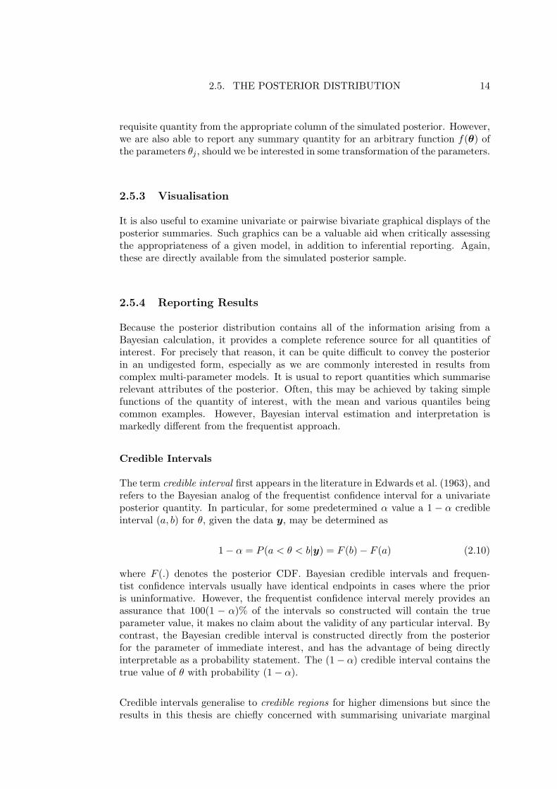
The term credible interval first appears in the literature in Edwards et al. (1963), andrefers to the Bayesian analog of the frequentist confidence interval for a univariateposterior quantity. In particular, for some predetermined α value a 1 − α credibleinterval (a, b) for θ, given the data y, may be determined as

1− α = P (a < θ < b|y) = F (b)− F (a) (2.10)

where F (.) denotes the posterior CDF. Bayesian credible intervals and frequen-tist confidence intervals usually have identical endpoints in cases where the prioris uninformative. However, the frequentist confidence interval merely provides anassurance that 100(1 − α)% of the intervals so constructed will contain the trueparameter value, it makes no claim about the validity of any particular interval. Bycontrast, the Bayesian credible interval is constructed directly from the posteriorfor the parameter of immediate interest, and has the advantage of being directlyinterpretable as a probability statement. The (1− α) credible interval contains thetrue value of θ with probability (1− α).

Credible intervals generalise to credible regions for higher dimensions but since theresults in this thesis are chiefly concerned with summarising univariate marginal


posterior quantities, such generalisations are not pursued. The interested readermay refer to Box and Tiao (1973).

While (2.10) allows the determination a credible interval (a, b) with credibility level(1−α), it does not specify uniquely defined endpoints. We describe two alternativemethods for determining specific univariate credible interval estimates.

Highest Posterior Density Intervals

The 100(1− α)% Highest Posterior Density (HPD) interval for θ is the set

C = {θ : p(θ|y) ≥ k(α)},

where k(α) is the largest constant such that

p(C|y) ≥ 1− α.

Figure 2.2: Disjoint Highest Posterior Density Interval.

Thus, the HPD interval provides the most likely values for θ, determined at the1 − α level. It will therefore also be the shortest credible interval which can beformed at that probability level. The definition allows the interval so formed to bedisjoint in cases of multi-modal posteriors where α is sufficiently large. For example,

2.6. CONCLUSION 16

the schematic diagram provided as Figure 2.2 shows the 80% HPD interval for amixture of normal distributions. The rigour provided by the HPD interval comesat a computational cost. Determination of k(α) against an arbitrary distributionrequires an iterative method to calculate the interval endpoints.

Equal Tail Intervals

A simpler approach to determine a specific credible interval can be found by takingthe interval such that “tails” of equal probability are excluded from the extremitiesof the marginal distribution for the quantity of interest.

Frequentist confidence intervals rely on an assumption of normality and this pro-vides symmetry: equal probability tails are supported by intervals of equal lengthon the support. No such symmetry is assumed in the Bayesian context, where theposterior distribution can take any form. In general the posterior will not be sym-metrical and excluding “tails” of equal probability implies the exclusion of unequalsegments at each end of the interval. For multi-modal or highly skewed posteriors,intervals based on the exclusion of equal tails may provide considerable differencesin support for θ from their HPD counterparts. However, for unimodal, moderatelyskewed distributions the difference between the intervals produced by the two meth-ods will be slight.

Thus, while recognising that HPD intervals are valuable in cases where the addi-tional computational burden is warranted, equal-tail intervals are used as the de-fault throughout this thesis. This also allows us to take advantage of the fact thatequal-tail intervals are readily available from the simulated posterior quantiles at noadditional computational expense.

2.6 Conclusion

In this chapter the basic principles of Bayesian analysis were introduced. Afterbriefly outlining the historical context of Bayesian methods, Bayes Theorem wasintroduced, and issues of interest regarding the prior and posterior distributionswere discussed, including the utility of conjugate forms and the nature of Bayesianinference and reporting. In summary, the following points are of interest:

• Bayesian methods have a (relatively) long history and well established pedi-gree. Despite controversies surrounding their use in the 20th century, there isno doubt regarding the mathematics of Bayes’ theorem.

• Bayesian methods deal with unknown quantities probabilistically. That is,unknown parameters are considered as random variables rather than fixed,unobservable quantities.

2.6. CONCLUSION 17

• Bayesian methods allow the practitioner to incorporate any prior informationregarding the probable values of a parameter into the probability calculus in aformal way. This powerful instrument is not available when using frequentistmethods. Significantly, it reflects the way in which practitioners of the scien-tific method generate knowledge about the world in real everyday situations.

• In cases where prior input has potential to influence outcomes, and the extentto which this is appropriate is in question, the Bayesian practitioner can electto repeat calculations using other prior distributions, including those whichprovide little or no information about likely parameter values. In this waythe degree to which prior beliefs impact results can be readily and reliablyassessed and reported.

• Bayesian analysis uses a single tool as the mechanism for calculating quan-tities of interest. Bayes theorem provides a consistent systematic approachto statistical inference. This contrasts with the frequentist approach whichuses a variety of methods depending on the context of the problem at hand,providing confusion to the novice user and making the tool set more difficultto master.

• Bayesian analysis allows direct interpretation of probability statements regard-ing parameters of interest. This is a compelling reason for the use of Bayestheorem, as casual users of statistics will interpret confidence intervals in thisway regardless of the mechanism used to generate them.

Having established the credentials of Bayesian methodology, we now turn to exam-ine their computational implementation.

Chapter 3

Bayesian Computation

3.1 Introduction

The choice of computational method for Bayesian analysis is largely dependent uponthe form of the posterior distribution. When the posterior is of known standard formsampling may be conducted directly by generating random deviates from the ap-propriate density. Such cases frequently arise from the adoption of conjugate priorsas discussed in §2.4.4.

In higher dimensional problems it may be possible to partition the parameter vector,for example as θ = (γ,φ), and factorise the posterior into manageable subcompo-nents

p(θ | y) = p(γ,φ | y) = p(γ | φ,y) p(φ | y), (3.1)

simulating each independently. However, as problems grow more complex posteriorforms tend to be non-standard and more sophisticated methods for constructingsamples must be employed.

In general, Bayesian methods are implemented via a Markov Chain Monte Carlo(MCMC) scheme, with the specific details of the scheme tailored to suit the natureof the target density. Samples can be drawn from arbitrary posterior distributionsbut the efficiency with which this may be achieved varies, depending upon the pos-terior form.

The present chapter aims to provide a brief sketch of MCMC methods, sufficient toestablish context for the applications found in later chapters. More detailed accountsof MCMC techniques appear in numerous texts. For example, Geyer (1992a); Gilkset al. (1995a) provide a general overview of the fundamental techniques and offermany suggestions for tuning these in various contexts. Gelman et al. (2003) discusscomputational aspects of Bayesian analysis integrated with an applied analyticaldevelopment. The work of Robert (1995) and Robert and Casella (2004), while

18

3.2. MARKOV CHAIN MONTE CARLO 19

not restricted solely to Bayesian analysis, covers computational issues relevant toimplementing MCMC in great detail, and thereby offers guidance in developingnovel applications. Congdon (2001) offers a plethora of worked examples from avariety of disciplines, all from a Bayesian MCMC perspective. Marin and Robert(2007) offer up to date practical advice on a range of applications.

3.2 Markov Chain Monte Carlo

The crux of MCMC methods is that under fairly general conditions it is possibleto construct a Markov chain which converges to a target density equivalent to theposterior distribution of the model in question (see, for example, Roberts, 1996).The posterior can then be described to any desired level of accuracy by samplingfrom the chain for sufficiently large number of iterations and using the ergodicaverage

E(f(X)) =1

n−m

n∑t=m+1

f(Xt) (3.2)

to form summary statistics for any quantity of interest. Bias introduced from sam-ples taken prior to convergence of the Markov chain is usually avoided by discardingan initial burn in count of iterations t ≤ m. Laws of large numbers ensure thatfor sufficiently large n, sample properties will reflect those of the population fromwhich the sample is taken. That is

limt→∞

1t

n∑t=m+1

Xt =∫ ∞−∞

xf(x) dx = E(X), (3.3)

where E(.) is the expectation operator. The next two sections describe, with in-creasing generality, how to construct such a Markov chain.

3.3 Gibbs Sampling

The Gibbs Sampler is an MCMC scheme which relies on partitioning the posteriorinto subcomponents, and simulating each of these in turn, conditional on the re-mainder. The scheme was introduced by Geman and Geman (1984), and brought toprominence in the statistical literature by Tanner and Wong (1987) and Gelfand andSmith (1990). Casella and George (1992), Smith and Gelfand (1992) and Gelfand(2000) provide accessible entry points into the literature.

Suppose we have a posterior which is the k dimensional joint probability distributionp(θ|y),θ = (θ1, θ2, . . . , θk), and interest lies in determining properties of the marginaldensity

3.4. METROPOLIS-HASTINGS SAMPLING 20

f(θ1) =∫. . .

∫f(θ1, θ2, . . . , θk) dθ2 . . . dθk. (3.4)

Gibbs sampling provides a method for obtaining a sample from f(θ1) without havingto evaluate (3.4) directly. And, by (3.3), taking a sufficiently large sample impliesthat any desired characteristic from f(θ1) can be determined with arbitrary preci-sion.

Writing θ−j for the vector with the jth component deleted (θ1, θ2, . . . , θj−1, θj+1, . . . , θk),the sample from f(θ1) is obtained by taking successive samples from each subcom-ponent of the posterior p(θj |θ−j ,y), and iterating such that

p(θtj | θt−1−j ,y) = p(θtj | θt1, θt2, . . . , θtj−1, θ

t−1j+1, . . . , θ

t−1k ,y), (3.5)

where the superscript t denotes the iteration count, until the required sample sizeis reached. That is, each subcomponent of the posterior is updated conditionallyusing the most recent values from the remaining subcomponents.

Gibbs sampling is efficient, since every sample generated is known to come fromthe target distribution p(θ|y), but is obviously only available for use in cases wherethe full conditional posterior can be determined analytically. In cases where theposterior is not available in this form a more general, albeit less efficient, samplingstrategy must be employed.

3.4 Metropolis-Hastings Sampling

The Metropolis-Hastings algorithm (3.6) provides a general regime allowing samplesto be drawn from an arbitrary target distribution p(θ|y). At each iteration a can-didate point θ∗ is sampled from a proposal distribution q(θ|y) and subjected to anacceptance test designed to admit proposed points into the sample with probabilityproportional to the density of p(θ|y) at θ∗. As with the Gibbs sampler, the processis iterated until a sample of the required precision is obtained.

The Metropolis algorithm was developed by Metropolis et al. (1953) and general-ized by Hastings (1970). Muller (1991) and Tierney (1994) provided articles whichbrought the process to the attention of the statistical mainstream. Chib and Green-berg (1995) and Gilks et al. (1995b) provide accessible introductory treatments.

The Metropolis-Hastings algorithm may be written as

3.4. METROPOLIS-HASTINGS SAMPLING 21

Initialise θ0

Loop {Sample θ∗ from q(θ∗ | θt−1)

Sample u from U(0, 1)

If u ≤ α(θ∗, θt−1)

θt = θ∗

else

θt = θt−1

Increment t

}

(3.6)

where U(0, 1) is the standard unit interval Uniform distribution, superscripts denoteiteration counts, and

α(θ∗, θt−1) = min(

1,p(θ∗) q(θt−1|θ∗)p(θt−1) q(θ∗|θt−1)

)(3.7)

defines the criteria for the acceptance test.

If we restrict our attention to the case of a symmetrical proposal distribution, asconsidered by Metropolis et al. (1953),

q(θt−1|θ∗) = q(θ∗|θt−1) (3.8)

and (3.7) simplifies to

α(θ∗, θt−1) = min(

1,p(θ∗)p(θt−1)

), (3.9)

from which the mechanics of the rejection process can be clearly understood. Whena proposed candidate θ∗ is closer to the mode of p(θ|y) than the current parametervalue θt−1, it will always be accepted since p(θ∗) ≥ p(θt−1). When the proposalcandidate is less probable than the current value it is accepted with probabilityappropriate to ensure that samples are drawn from p(θ|y).

Of course, when p(θ∗) ≤ p(θt−1) the acceptance rate is directly proportional to theratio of the terms in this inequality, so choice of proposal distribution is critical forefficient sampling. Indeed, the efficiency of Gibbs sampler can now be plainly seen,since the proposal and target distributions are equivalent for the full conditionalcase, and rejection never occurs.

3.5. DIAGNOSING CONVERGENCE 22

The additional generality of asymmetry in q(.) supplied by Hastings (1970) modifiesthe acceptance rate using the ratio of ratios

p(θ∗) / q(θ∗|θt−1)p(θt−1) / q(θt−1|θ∗)

(3.10)

which normalise the numerator and denominator according to the degree of asym-metry in the proposal distribution and provide the full generality of (3.7).

The Metropolis-Hastings algorithm describes how samples from an MCMC simula-tion may be obtained to provide inference regarding an arbitrary posterior, assumingthat the Markov chain converges to the required target distribution p(θ|y). It can beshown, Robert and Casella (see, for example, 2004) that the stationary distributionof the Markov chain so generated is the required target distribution.

3.5 Diagnosing Convergence

Convergence of an MCMC chain to the target distribution is difficult to establish.There is no specific test which can be performed to indicate that convergence hasbeen achieved, and in practice diagnosis tends to be negatively defined: one looksfor signs of non-convergence and in the absence of these assumes that the chain hassatisfactorily converged.

A number of diagnostics to aid the detection of convergence have been put forward,starting with Heidelberger and Welch (1981), Schruben (1982) and Heidelberger andWelch (1983). Establishing convergence metrics remained a controversial topic inthe MCMC literature throughout the 1990’s, with a prominent suggestion put for-ward by Gelman and Rubin (1992, modified, and generalised, in Brooks and Gelman(1998)), and criticised by Geyer (1992a,b). Other input to the debate was providedby Geweke (1992), Raftery and Lewis (1992, 1995), Gelman (1995), Cowles andCarlin (1996), and Kass et al. (1998), and the many references therein.

3.5.1 Gelman and Rubin’s R

Gelman and Rubin (1992) propose a general approach to monitoring the convergenceof MCMC output using m > 1 chains with overdispersed starting values. Chains arediagnosed as having converged when the influence of the initial values is no longerevident. That is, the output from the multiple chains is effectively indistinguishable.The specific diagnostic tool used for this purpose uses a comparison of the within-and between-chain variances, essentially providing an anova style statistic.

There are two estimates for the variance of the stationary distribution representedby the MCMC output, the mean of the m within-sequence variances s2i


W =m∑i=1

s2i /m (3.11)

and the empirical variance from all chains combined

σ2 =(n− 1)W

n+B

n, (3.12)

where

B/n =m∑i=1

(xi. − x..)/(m− 1), (3.13)

the variance between the m sequence means xi.. If the chains have converged, bothestimates are unbiased. If not, (3.11) will be an underestimate, since the chains havenot had sufficient opportunity to explore the full support of the posterior, and (3.12)will overestimate the variance, since the started values of the chain were chosen tobe overdispersed.

Then, using the assumption that the posterior can be approximated by a normaldistribution with estimated mean and variance, a t-distribution can be used toconstruct a Bayesian credible interval with mean

µ =1mn

m∑i=1

n∑j=1

xij ,

variance

V = σ2 +B

mn,

and degrees of freedom

d =2V 2

var(V ),

with var(V ) estimated by the method of moments. Finally, the convergence diagnos-tic itself is the ratio of the current variance estimate V to the within-chain varianceestimate W , with an adjustment factor to account for the additional variance in thet-distribution,

R =V

W.d+ 3d+ 1

. (3.14)

This provides an estimate of the factor by which the scale of the current distributionfor x might be reduced if the chain were allowed to continue indefinitely n→∞. If


R is substantially greater than unity, there is reason to believe that further iterationof the chain will improve inference regarding the posterior target. That is, Bayesiancredible intervals based on the t-distribution have the potential to shrink by a fac-tor of R. Brooks and Gelman (1998) updated the original diagnostic of Gelmanand Rubin (1992) to the form indicated in (3.14), and generalized this for use withmultiple parameters simultaneously.

3.5.2 Discussion

Despite the reassurances implicit in diagnostic statistics such as Gelman and Ru-bin’s R, a simple quantitative diagnostic to detect Markov chain convergence provesto be an elusive problem. Cowles and Carlin (1996), for example, surveyed thirteenconvergence diagnostics and found that each of them failed to detect the type ofnon-convergence they were designed to identify in two simple models. Kass et al.(1998) discuss a range of issues related to the implementation of MCMC includingthe difficulties associated with convergence diagnosis, and use of the R diagnosticpresented in Gelman and Rubin (1992). The discussion raises a number of difficultiesto the development of robust convergence diagnostics related to qualitative differ-ences in chain behaviour associated with starting values, model misspecification,and uncertainties in model choice; highlighting the fact that diagnosing convergenceis not a straightforward issue.

The position adopted in this thesis is one of eclecticism. In keeping with Neal fromKass et al. (1998) we elect to run a small number of chains and monitor these usingGelman and Rubin’s R, and in addition visually inspect the chain trace from eachsimulated variable for signs of poor mixing or divergence, under the assumptionthat careful visual monitoring of qualitative trends is an instructive supplementto diagnostic metrics. The implementation of the updated version of Gelman andRubin’s R (3.14) provided in the coda package (Plummer et al., 2009) of the Rstatistical environment was used throughout, in combination with visual inspectionbased on the principles outlined in the next section.

3.5.3 Mixing

In order for the sample generated from an MCMC scheme to reflect the propertiesof the posterior distribution, it must visit the entire support of the posterior inproportions reflecting the posterior density. The degree to which this is achievedcan be assessed by inspection of the MCMC chain trace, which thus provides a usefulqualitative measure of performance. As Geyer (1992a) points out, inspection of thechain trace will only identify some forms of problem behaviour, but in practicewe find it a useful supplement to quantitative diagnostics. Examples of typicalsituations of interest are shown in Figure 3.1.


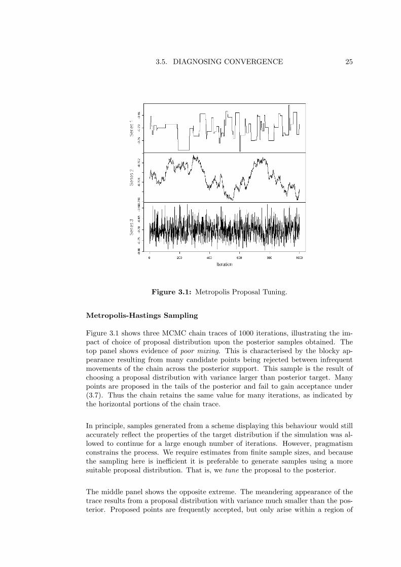
Figure 3.1: Metropolis Proposal Tuning.

Metropolis-Hastings Sampling

Figure 3.1 shows three MCMC chain traces of 1000 iterations, illustrating the im-pact of choice of proposal distribution upon the posterior samples obtained. Thetop panel shows evidence of poor mixing. This is characterised by the blocky ap-pearance resulting from many candidate points being rejected between infrequentmovements of the chain across the posterior support. This sample is the result ofchoosing a proposal distribution with variance larger than posterior target. Manypoints are proposed in the tails of the posterior and fail to gain acceptance under(3.7). Thus the chain retains the same value for many iterations, as indicated bythe horizontal portions of the chain trace.

In principle, samples generated from a scheme displaying this behaviour would stillaccurately reflect the properties of the target distribution if the simulation was al-lowed to continue for a large enough number of iterations. However, pragmatismconstrains the process. We require estimates from finite sample sizes, and becausethe sampling here is inefficient it is preferable to generate samples using a moresuitable proposal distribution. That is, we tune the proposal to the posterior.

The middle panel shows the opposite extreme. The meandering appearance of thetrace results from a proposal distribution with variance much smaller than the pos-terior. Proposed points are frequently accepted, but only arise within a region of

3.6. CONCLUSION 26

the posterior which is proximal to the current value of the chain. A chain with thischaracteristic fails to visit the support of the posterior in appropriate proportions.

The lower panel shows 1000 samples from the same posterior with a well tuned pro-posal distribution. Samples are obtained from the entire support of the posterior inproportion to the posterior density.

Gibbs Sampling

In the case of Gibbs sampling, the posterior distribution is the proposal distribution,the probability of acceptance of any candidate point is 1, and the situation in thetop panel of Figure 3.1 can never arise, because rejection never occurs. However,behaviour similar to that indicated by the middle panel can still arise, particularlywhen the simulated estimands are are highly correlated. In such cases movementsin any direction other than the main axis of the posterior are relatively improbable,and so sampling schemes which update one variable at a time can become “trapped”in restricted regions of the posterior for an unacceptable number of iterations. So-lutions for dealing with such contingencies will be introduced on a case wise basisas necessary throughout.

We will frequently employ more than one chain to assist in the assessment of mixing.Doing so provides a check that the regions of the support visited by both chainsare approximately equal, and in satisfactory circumstances these chains will provideindependent samples from the posterior.

3.6 Conclusion

This chapter has provided background material to the implementation of MarkovChain Monte Carlo sampling schemes. We saw that in cases where the posteriorcould be appropriately partitioned and full conditional distributions could be ana-lytically determined, Gibbs sampling provides an efficient means of drawing samplesfrom marginal components of the posterior. In cases where these requirements couldnot be met, Metropolis-Hastings sampling allows samples to be drawn from an ar-bitrary posterior, at the expense of some efficiency. After an initial outline of thedesirability of detecting convergence, a detailed description of Gelman and Rubin’sconvergence diagnostic was provided. We opt for checking the value of this metric inaddition to visual inspection of the MCMC chain trace. The advantage of the latteris that it allows for a qualitative assessment of the mixing characteristics of thechains. The concept of “tuning” a proposal distribution to achieve adequate mixingof the MCMC chain was also described for use in cases employing Metropolis-basedsampling regimes, and a similar problem scenario identified for the Gibbs samplingcase. We now turn to the application of these procedures in problems of substantiveinterest.

Chapter 4

Nonlinear Regression Models

4.1 Introduction

Nonlinear regression extends the general linear model by allowing the expected con-ditional response to take a nonlinear form. This flexibility presents a dilemma. Oncearbitrary parametric functions are admissible for the model mean, many alternativeparameterisations of the basic functional form will be available. On what basis arealternative candidates best selected?

Historically, researchers have taken a necessarily pragmatic view of this problem: pa-rameterisations were chosen on the basis of enabling numerical methods to converge,and preference given to those parameterisations which produced approximately nor-mal sampling distributions for the estimators, as these were required to minimiseinferential bias in asymptotically justified confidence intervals.

Early accounts investigating nonlinear regression are due to Beale (1960), Hartley(1961), Marquardt (1963), Hartley and Booker (1965), Jennrich (1969), and Gallant(1975). Ratkowsky (1983), Gallant (1987), and Ross (1990) offer practical advice,Bates and Watts (1988) and Seber and Wild (2003) offer more comprehensive treat-ments.

This chapter presents Bayesian MCMC as an alternative to Least Squares methodsfor nonlinear regression. In many situations, the basic MCMC apparatus presentedin the introductory chapters can be applied in a straightforward way. We re-examinethe growth curve models presented in Ratkowsky (1983) to establish the applicabil-ity of the MCMC approach, and explore the details of problem cases to establish thelimitations of naıve application of the technique, and provide guidance in surmount-ing obstacles. MCMC provides advantages when faced with difficulties of choosingbetween alternative parameterisations. We show that the availability of posteriorsamples obtained under one parameterisation allows estimation and inference re-garding alternative parameterisations.

27

4.2. LINEAR REGRESSION MODELS 28

4.2 Linear Regression Models

Throughout most of the 20th century the general linear model formed the mainstayof statistical practice, and it continues to be of central importance. Indeed, manyof the modelling frameworks which have come to fruition in recent decades areextensions to the general linear form, arising from relaxing or generalizing one ormore of the assumptions upon which the general linear model rests

1. The mean response is a linear function of the predictors.

2. Model residuals are conditionally independent.

3. Model residuals are distributed with conditional mean zero.

4. Model residuals have constant conditional variance.

5. Model residuals are conditionally normal in distribution.

The criteria 2–5 are often represented more compactly as

εiiid∼ N (0, σ2) (4.1)

where εi is the ith model residual, the ∼ symbol is read “distributed as”, iid standsfor identically and independently distributed, and N (0, σ2) is the normal distribu-tion with mean zero and standard deviation σ.

It is common to suppress the conditionality of the criteria when writing the model,so that we encounter the linear model as

yi = β0 +∑

βjxj + εi (4.2)

where yi, i = 1, . . . , n, is the ith observation, xj , j = 1, . . . , p−1,is the jth covariate,βk, k = 0, . . . , p − 1 is the kth parameter to be estimated, and the model residualsεi meet the criteria specified in (4.1). Model fitting focuses upon estimation of, andinference regarding, the parameters β.

The residual sum of squares (RSS) is a measure of model fit, and represents thevariability in the data which remains unexplained by the model. Specifically, RSSis the squared sum of deviations from the model mean

RSS = S(β) =n∑i=1

ε2i =n∑i=1

[Yi − (β0 +∑

βjxj)]2, (4.3)

where β is chosen so as to minimise (4.3).

4.3. NONLINEAR REGRESSION MODELS 29

Alternatively, we might choose to view (4.2) in terms of the likelihood that param-eters take on particular values. The criteria (4.1) determine the likelihood functionfor (4.2)

l(β, σ) ∝ σ−ne−S(β)/2σ2, (4.4)

where the model parameters β are chosen to maximise the likelihood. From (4.3)and (4.4) we see that both are functions of the model parameters β, and that min-imising the residual sum of squares (4.3) is equivalent to maximising the likelihoodfunction (4.4).

Least Squares estimates for β are obtained by setting partial derivatives of (4.3)equal to zero with respect to each βk, k = 0, 1, . . . , p− 1,

∂S(β)∂βk

= 0 (4.5)

and solving the resultant normal equations for the respective βk.

The key feature of (4.2) is that the terms involving β are additive: the model is linearin its parameters. This in turn implies that the solutions to the normal equationsare linear combinations of the observations. Writing the general solution in matrixnotation

β = (XTX)−1XTY (4.6)

one can plainly see that the parameter estimates β rely only upon X and Y .

4.3 Nonlinear Regression Models

Nonlinear regression allows for criterion one from §4.2 to be relaxed so that themodel mean is no longer required to be a linear function of the covariates. Toemphasise this difference, it is customary to adopt a different notation, and wecommonly see nonlinear models written as

yu = f(ξ;θ) + εu (4.7)

where yu, u = 1, . . . , n, is the uth observation, ξ is a vector of covariate values,f(ξ;θ) is an arbitrary function of the covariates parameterised by the vector θ, andthe model residuals εu meet the criteria specified in (4.1). Model fitting focusesupon estimation of, and inference regarding, the model parameters θ.

As previously, (4.1) ensures equivalence between Least Squares and Maximum Like-lihood estimates of θ. However, in the nonlinear case the Least Squares estimate θrequires minimisation of the residual sum of squares

4.4. NONLINEAR REGRESSION USING MCMC 30

S(θ) =n∑u=1

{yu − f(ξ,θ)}2, (4.8)

and here the normal equations take the form

∂S(θ)∂θk

=n∑u=1

{yu − f(ξ, θ)}[∂f(ξ,θ)∂θk

]θ=θ

= 0. (4.9)

Unlike the linear case, (4.9) is a function of the model parameters θ. Thus, whenthe model is nonlinear in θ, the normal equations are also nonlinear in θ. Thisrenders them much more difficult to solve.

Least Squares estimation of model parameters in nonlinear regression often relieson iterative numerical techniques, such as the Gauss-Newton (Hartley, 1961; Draperand Smith, 1998) or Newton-Raphson methods (Marquardt, 1963; Chambers, 1973;Ratkowsky and Dolby, 1975). These techniques estimate θ by repeatedly solvinglinearized forms of f(.) in restricted local regions around the current estimated val-ues θ. It is often necessary to provide routines with starting values approximatingthe final estimates to enable convergence, and determining these is something of anart.

Moreover, the estimators obtained using these procedures are known to be biased,with the extent of that bias determined by what Bates and Watts (1980, 1988)(following Beale, 1960) describe as the “intrinsic nonlinearity” of the model – datacombination. Additional bias may be introduced by the choice of parameterisationof f(.) in (4.7) (Bates and Watts, 1981; Cook and Witmer, 1985; Cook and Gold-berg, 1986). Further, confidence intervals for these estimators rely on asymptoticassumptions of normality (Clarke, 1987; Chen and Jennrich, 1995), which may onlybe reasonably approximated by sample sizes which are beyond those typically avail-able to researchers in biology, agriculture, and other applied fields. In summary,nonlinear regression poses considerable challenges to the non-specialist. Indeed,Ratkowsky (1983) provides a book length treatment on how to achieve reasonableresults.

4.4 Nonlinear Regression using MCMC

Given the established difficulties of nonlinear regression, and the promise of a gen-eral purpose modelling framework such as MCMC, it seems natural to consider howwe might apply MCMC to nonlinear parameter estimation.

We developed a basic MCMC procedure based on the Metropolis-Hastings algo-rithm (3.6), with a univariate normal proposal distribution for each parameter. Avery simple adaptive mechanism was used to tune the proposal to the posterior asdescribed in the next section. We begin by considering a simple example to establish


the basic use of the method.

4.4.1 Example: Biochemical Oxygen Demand

Biochemical oxygen demand (BOD) is used as a measure of environmental pollutioncaused by anthropogenic wastes. Typically a small quantity of the waste materialis mixed with pure water and sealed in a container which is incubated at a fixedtemperature for a small number of days. The reduction of the dissolved oxygen inthe water allows calculation of the BOD, in units of mg/l, during the incubationperiod.

# Day BOD1 1 0.472 2 0.743 3 1.174 4 1.425 5 1.606 7 1.847 9 2.198 11 2.17

Table 4.1: Biochemical Oxygen Demand DataSource: Bates and Watts (1988)

Bates and Watts (1988) consider the BOD data provided in Table 4.1 and fit thefunction

f(x;θ) = α(1− e−βx), (4.10)

where f is predicted biochemical oxygen demand, and x is time. We demonstratean MCMC parameter estimation procedure by fitting (4.10) to these data.

Initialisation

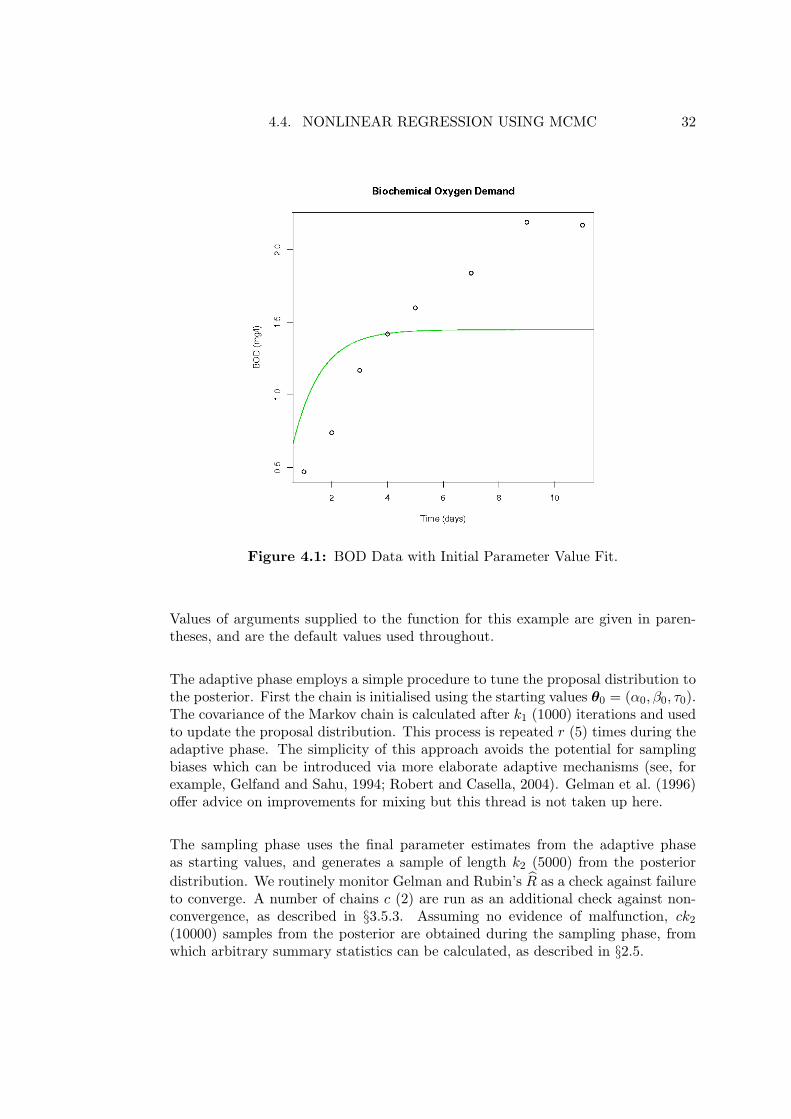
Figure 4.1 shows the BOD data with a curve depicting the fit of the initial param-eter values passed to the MCMC procedure: the mean BOD value α0 = 1.45, anda rate parameter β0 = 1. Obviously these starting values provide a poor fit to thedata. A starting value for the precision is also required, here τ0 = 4.

Operation

The MCMC method consists of two phases: an adaptive phase (see, for example,Gilks et al., 1994; Gilks and Roberts, 1995; Fearnhead, 2008) and a sampling phase.


Figure 4.1: BOD Data with Initial Parameter Value Fit.

Values of arguments supplied to the function for this example are given in paren-theses, and are the default values used throughout.

The adaptive phase employs a simple procedure to tune the proposal distribution tothe posterior. First the chain is initialised using the starting values θ0 = (α0, β0, τ0).The covariance of the Markov chain is calculated after k1 (1000) iterations and usedto update the proposal distribution. This process is repeated r (5) times during theadaptive phase. The simplicity of this approach avoids the potential for samplingbiases which can be introduced via more elaborate adaptive mechanisms (see, forexample, Gelfand and Sahu, 1994; Robert and Casella, 2004). Gelman et al. (1996)offer advice on improvements for mixing but this thread is not taken up here.

The sampling phase uses the final parameter estimates from the adaptive phaseas starting values, and generates a sample of length k2 (5000) from the posteriordistribution. We routinely monitor Gelman and Rubin’s R as a check against failureto converge. A number of chains c (2) are run as an additional check against non-convergence, as described in §3.5.3. Assuming no evidence of malfunction, ck2

(10000) samples from the posterior are obtained during the sampling phase, fromwhich arbitrary summary statistics can be calculated, as described in §2.5.


Figure 4.2: Adaptive MCMC Trace: BOD Model.

Diagnostics

During either phase of the MCMC procedure diagnostic plots can be used to visuallycheck for signs of non-convergence. Figures 4.2 and 4.3 show the chain traces forthe adaptive and sampling phases of the BOD example.

The first 1000 iterations of Figure 4.2 show obvious symptoms of instability, mostclearly indicated by the divergent chain traces for τ . The chains for both α and βalso show maximum variability during this portion of the trace. At iteration 1001,the chains have been restarted with an updated proposal distribution using the co-variance of the previous 1000 iterations. This improves the efficiency of acceptance,and results in reduced variability in the traces for α and β, and better mixing for theprecision parameter τ . A second restart at iteration 2001, with the proposal usingthe covariance of the values generated in iterations [1001, 2000], appears sufficient tohave stabilised the sampling process, none of the parameters indicate problematicsymptoms past this point.

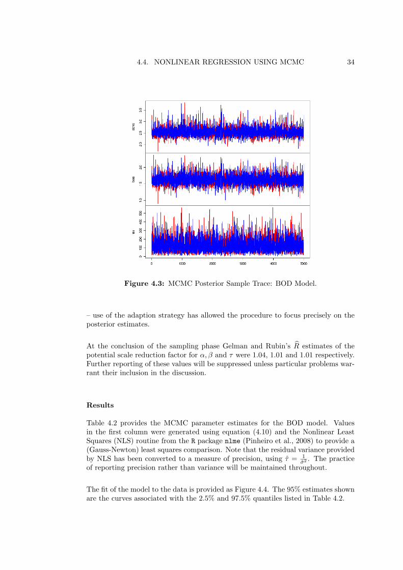
Figure 4.3 shows the sample trace obtained by running the MCMC routine usinga proposal based on the covariance estimate from the final 1000 iterations of theadaptive phase as starting values. Again, no symptoms of non-convergence are ev-ident, and 10,000 posterior samples have been obtained for each parameter. Notealso the change in scale for parameters α and β between this and the previous figure


Figure 4.3: MCMC Posterior Sample Trace: BOD Model.

– use of the adaption strategy has allowed the procedure to focus precisely on theposterior estimates.

At the conclusion of the sampling phase Gelman and Rubin’s R estimates of thepotential scale reduction factor for α, β and τ were 1.04, 1.01 and 1.01 respectively.Further reporting of these values will be suppressed unless particular problems war-rant their inclusion in the discussion.

Results

Table 4.2 provides the MCMC parameter estimates for the BOD model. Valuesin the first column were generated using equation (4.10) and the Nonlinear LeastSquares (NLS) routine from the R package nlme (Pinheiro et al., 2008) to provide a(Gauss-Newton) least squares comparison. Note that the residual variance providedby NLS has been converted to a measure of precision, using τ = 1

σ2 . The practiceof reporting precision rather than variance will be maintained throughout.

The fit of the model to the data is provided as Figure 4.4. The 95% estimates shownare the curves associated with the 2.5% and 97.5% quantiles listed in Table 4.2.


MCMC QuantilesNLS Mean σ 50% 2.5% 97.5%

α 2.4979 2.5318 0.1861 2.5129 2.2200 2.9544β 1.5972 1.6158 0.1437 1.6097 1.3468 1.9177τ 228.6265 129.3753 73.6373 114.9239 27.5127 309.5821

Table 4.2: Summary Statistics: BOD Data Model.

Discussion

One of the key advantages of using MCMC to simulate the posterior distributionis that the posterior samples remain available for subsequent use. As discussed in§2.5.2, inference in the Bayesian context is simply a matter of summarising poste-rior quantities of interest. The summary statistics seen in Table 4.2, for example,were generated directly from the posterior samples. However, the availability ofthese samples also provides the ability to visualise the sampling distributions of themodel parameters.

Figure 4.5 shows the pairwise marginal scatterplots of the posterior distribution forthe BOD model. From these plots we can see that α and β are highly correlated,that α shows greater positive skew than β and that the joint posterior distributionof these parameters exhibits curvature, a feature that shall become important laterin the chapter. The distinctive conical shape associated with τ in these diagramsindicates that high values of precision (low variance) are correlated with the poste-rior mode.

Having established the utility of the MCMC method, we now turn to consider itsperformance relative to Least Squares in the context of growth curve models.


Figure 4.4: Fitted BOD Model.

Figure 4.5: Pairwise Marginal Scatterplots: BOD Model.

4.5. GROWTH CURVE MODELS USING MCMC 37

4.5 Growth Curve Models using MCMC

4.5.1 Ratkowsky’s Regression Strategy

Ratkowsky (1983) developed a strategy for nonlinear regression based on the dis-tinction made by Bates and Watts (1980, 1988) between intrinsic nonlinearity, at-tributable to the functional form of the model, and parameter effects nonlinearity,attributable to the chosen parameterisation within that functional form. Hougaard(1982) and Kass (1984), among others, have also considered parameterisation issues.

Ratkowsky argued that model parameterisations which perform in a “close to linear”fashion are preferable. The sampling distributions of the least squares estimatorsapproximate normality more closely in such cases, are therefore less biased, and pro-vide a more reliable basis for the calculation of confidence intervals. A significantadditional benefit is that convergence of the numerical routines employed is oftenfacilitated when the sampling distributions of the parameters approximate normaldistributions.

These arguments are appealing in the context of Least Squares, where approximatelynormal sampling distributions are required for the asymptotic theory of inference tohold. However, MCMC allows this requirement to be relaxed. The credible intervalsintroduced in §2.5.4 can be obtained from the any posterior distribution, regardlessof form. Moreover, as we have seen, the availability of posterior samples allowsready calculation of any summary quantity desired. Significantly, this provides theability to transform estimates between alternative parameterisations of a model,leaving the practitioner free to explore model parameterisations motivated by crite-ria other than the necessity that it may be the only mathematically tractable option.

4.5.2 Model Functions and Data

Ratkowsky (1983) considers five nonlinear growth curve types; two three-parametercases: the Gompertz (4.11) and logistic (4.12) model functions

y = α exp[−exp(β − γx)], (4.11)

and

y =α

1 + exp(β − γx), (4.12)

and three four-parameter cases, the Morgan-Mercer-Flodin (MMF) (4.13), Richards(4.14), and Weibull-type (4.15) model functions

y =βγ + αxδ

γ + xδ, (4.13)


# x y

1 0.50 1.302 1.50 1.303 2.50 1.904 3.50 3.405 4.50 5.306 5.50 7.107 6.50 10.608 7.50 16.009 8.50 16.4010 9.50 18.3011 10.50 20.9012 11.50 20.5013 12.50 21.3014 13.50 21.2015 14.50 20.90

Table 4.3: Bean DataSource: Heyes and Brown (1956), cited in Ratkowsky (1983)

y =α

[1 + exp(β − γx)]1δ

, (4.14)

and

y = α− β exp(−γxδ), (4.15)

where y is a vector of responses, x is a vector of covariate data, and θ = (α, β, γ),or θ = (α, β, γ, δ), is a vector of parameters to be estimated.

# x y

1 0.00 1.232 1.00 1.523 2.00 2.954 3.00 4.345 4.00 5.266 5.00 5.847 6.00 6.218 8.00 6.509 10.00 6.83

Table 4.4: Cucumber DataSource: Gregory (1956) cited in Ratkowsky (1983)


# x y

1 1.00 16.082 2.00 33.833 3.00 65.804 4.00 97.205 5.00 191.556 6.00 326.207 7.00 386.878 8.00 520.539 9.00 590.0310 10.00 651.9211 11.00 724.9312 12.00 699.5613 13.00 689.9614 14.00 637.5615 15.00 717.41

Table 4.5: Onion DataSource: Gregory (1956) cited in Ratkowsky (1983)

Each of these model functions was applied to four datasets related to vegetativegrowth processes, providing an initial set of 20 cases of interest. These data are pro-vided in Tables 4.3 - 4.6, and will be referred to as the Bean (Table 4.3), Cucumber(Table 4.4), Onion (Table 4.5) and Pasture (Table 4.6) data respectively.

A similar approach will be followed here. Each of the 20 initial data – model func-tion combinations were evaluated using the MCMC procedure described in §4.4.1.The results are categorised by the model function type listed above.

# x y

1 9.00 8.932 14.00 10.803 21.00 18.594 28.00 22.335 42.00 39.356 57.00 56.117 63.00 61.738 70.00 64.629 79.00 67.08

Table 4.6: Pasture DataSource: Ratkowsky (1983)


4.5.3 Three Parameter Models

Logistic & Gompertz Models

Figure 4.6: Fitted Gompertz-Cucumber Model.

MCMC parameter estimates using the Gompertz (4.11) and logistic (4.12) modelfunctions for each data set are provided in Tables 4.7 and 4.8. The results obtainedby Ratkowsky (1983) are provided in the first column for comparison, with variancesconverted to precisions as previously noted. In each case the parameter estimatereported by Ratkowsky (1983) falls within the 95% credible interval obtained usingthe MCMC procedure. These tables reaffirm that the MCMC procedure is capa-ble of producing results comparable with those obtained by nonlinear Least Squares.

Assessing Model Fit

In Tables 4.7 and 4.8 the precision estimates τ obtained using MCMC are compara-ble with those reported by Ratkowsky (1983). However, using precision as the solecriterion of model fit is problematic, and it needs to be interpreted with care. Forexample, Tables 4.7 and 4.8 show the precision estimates for the Cucumber modelsto be large relative to the other datasets, across both model functions and bothestimation methods. By contrast, the precision estimates for the Onion data sug-gest that both methods of estimation produce models which fail to fit the data well.Visualising the fit of the models corresponding to the Gompertz cases in Figures


MCMC QuantilesRatkowsky Mean σ 50% 2.5% 97.5%

Bean Data:

α 22.5100 22.4333 0.9108 22.3869 20.7853 24.4382β 2.1060 2.2127 0.3635 2.1646 1.6675 3.0485γ 0.3880 0.4067 0.0644 0.3996 0.3050 0.5582τ 0.9533 0.9358 0.3910 0.8840 0.3321 1.8462

Cucumber Data:

α 6.9250 6.8711 0.3426 6.8948 6.0185 7.4349β 0.7680 0.9432 0.9230 0.7861 0.5672 2.5750γ 0.4930 0.5839 0.4445 0.5050 0.3911 1.5406τ 16.1551 15.8105 10.1483 13.8672 1.1566 40.6648

Onion Data:

α 723.1000 720.8077 23.9323 719.8647 676.1035 770.6005β 2.5000 2.5910 0.3574 2.5577 1.9896 3.4062γ 0.4500 0.4663 0.0628 0.4608 0.3609 0.6055τ 0.0009 0.0009 0.0004 0.0008 0.0003 0.0017

Pasture Data:

α 82.8300 83.6054 6.3747 82.9106 72.5160 97.6067β 1.2240 1.2341 0.0942 1.2244 1.0769 1.4427γ 0.0370 0.0373 0.0050 0.0371 0.0288 0.0482τ 0.2755 0.2863 0.1609 0.2563 0.0633 0.6907

Table 4.7: Summary Statistics: Gompertz Models.



Bean Data:

α 21.5100 21.4892 0.4514 21.4892 20.6151 22.4068β 3.9570 4.0229 0.3160 3.9984 3.4709 4.7196γ 0.6220 0.6333 0.0534 0.6297 0.5402 0.7511τ 1.9305 1.9191 0.7955 1.8044 0.6992 3.7551

Cucumber Data:

α 6.6870 6.6747 0.1804 6.6727 6.3374 7.0305β 1.7450 1.7731 0.1738 1.7625 1.4579 2.1589γ 0.7550 0.7706 0.0796 0.7650 0.6303 0.9447τ 28.3286 25.7820 14.7332 23.0487 5.2821 62.0883

Onion Data:

α 702.9000 701.9848 15.0409 701.6988 671.9047 732.7782β 4.4430 4.5246 0.3959 4.4986 3.8082 5.3896γ 0.6890 0.7023 0.0636 0.6990 0.5889 0.8411τ 0.0013 0.0013 0.0005 0.0013 0.0005 0.0026

Pasture Data:

α 72.4600 72.6086 2.2411 72.4511 68.7950 77.1946β 2.6180 2.6270 0.1072 2.6235 2.4255 2.8501γ 0.0670 0.0675 0.0041 0.0675 0.0595 0.0759τ 0.7463 0.7335 0.4181 0.6560 0.1512 1.7412

Table 4.8: Summary Statistics: Logistic Models.


Figure 4.7: Fitted Gompertz-Onion Model.

4.6 and 4.7 reveal this interpretation to be flawed. The Onion models appear to fitbetter than the Cucumber models.

Faced with this apparent contradiction it is tempting to think that posterior vari-ability should provide a useful guide. After all, the wide 95% credible intervalassociated with τ in the Gompertz – Cucumber case suggests that we might expectthe model to fit less well. However, the Logistic – Cucumber model also reports awide credible interval for τ , and inspection of the fitted model for that case (Figure4.8) reveals no suggestion of ill fit. These examples highlight the fact that it isinadvisable to make comparisons between nonlinear models on the basis of simplesummary statistics. As Seber and Wild (2003) point out, the relative magnitudesof residual variances vary with the model – data combination on a casewise basis innonlinear regression.

Diagnostics

The previous section revealed the fit of the Gompertz – Cucumber model (Figure4.6) to be unsatisfactory. Because the MCMC posterior samples are available, di-agnosis of the problem is straightforward.

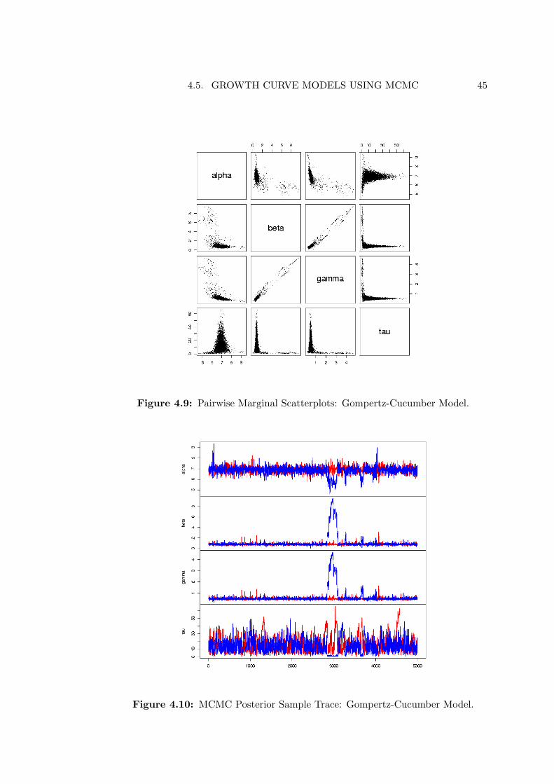
Scatterplots of the pairwise marginal posterior slices for the Gompertz – Cucumbermodel parameters are provided in Figure 4.9. High values of precision are asso-


Figure 4.8: Fitted Logistic-Cucumber Model.

ciated with the mode of each parameter estimate, as expected. But there is alsoa large low density region distant from the mode corresponding to very low preci-sion values. Inspection of the MCMC sample trace provides further insight. Figure4.10 reveals a major excursion away from the main density of the posterior by onechain around iteration 3000. This is correlated with a period of low precision and,along with some later minor excursions, is responsible for the large low density ar-eas observed in the pairwise marginal plots. Armed with these diagnostic aids, wemay choose to re-run the procedure to produce a more satisfactory posterior sample.

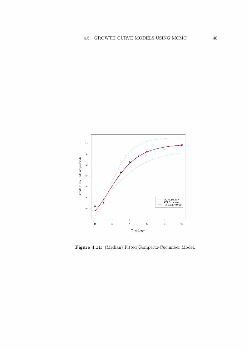
However, because these excursions are minor aberrations among 10000 samples, wemight expect the existing median estimates to be robust to their influence. Themodel fit using the MCMC median values from Table 4.7 is provided in Figure 4.11,and attests the adequacy of these values.


Figure 4.9: Pairwise Marginal Scatterplots: Gompertz-Cucumber Model.

Figure 4.10: MCMC Posterior Sample Trace: Gompertz-Cucumber Model.


Figure 4.11: (Median) Fitted Gompertz-Cucumber Model.


4.5.4 Four Parameter Models

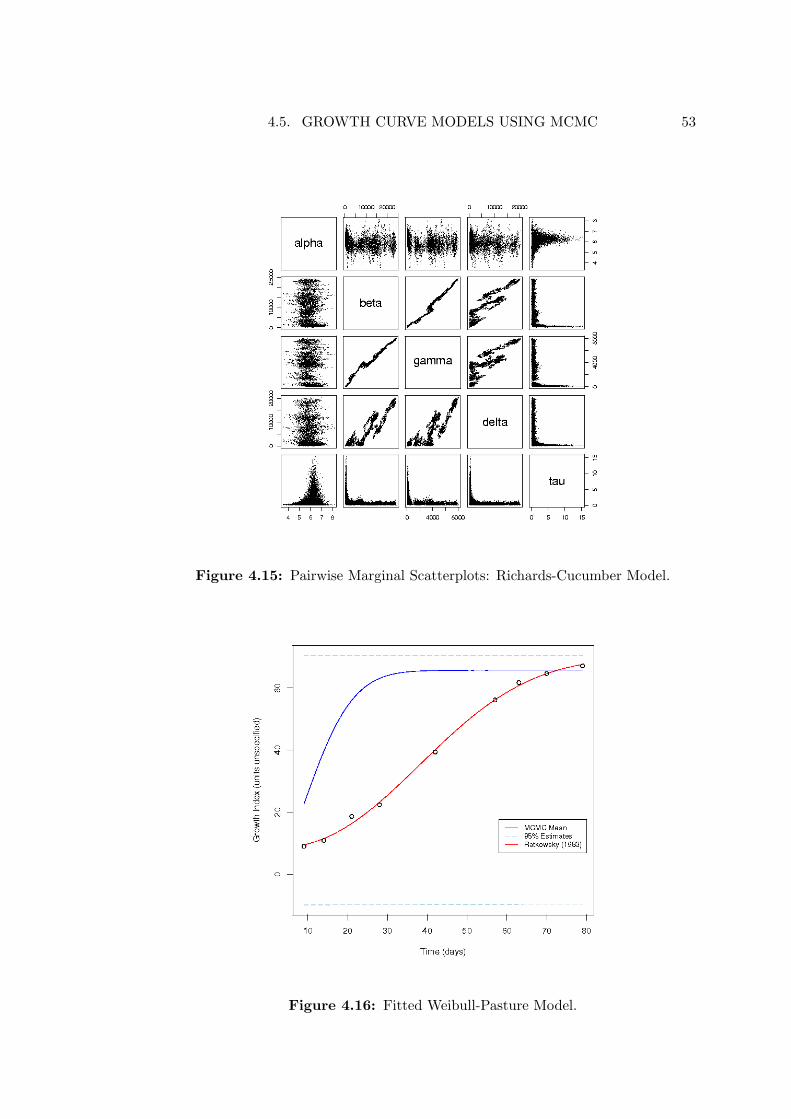
Estimates from the four parameter models (4.13) – (4.15) are provided in Tables 4.9,4.10 and 4.11. The performance of each model function will be evaluated in turn.In the interests of brevity exhaustive details of all 20 cases will be omitted, otherthan reporting the summary statistics in the tables listed above. Instead, we focuson cases where the MCMC method did not perform well, with a view to diagnosis.

Morgan-Mercer-Flodin Models

Figure 4.12: Fitted MMF-Cucumber Model.

The estimates for the MMF model function are provided in Table 4.9. Direct com-parison of the estimates reported in the first two columns may be misleading. Themean MCMC estimates for many of the parameters appear to approximate theirNLS counterparts only roughly, and γ is frequently out by a factor of two. However,visualising the fit of the models against the data reveals that the differences are notas severe as might be expected based on the comparative estimates. The Cucumbermodels (Figure 4.12), for example, are in excellent agreement despite the large re-ported difference in values for τ . By contrast, the fitted models for the Onion datareport identical precisions and are shown in Figure 4.13. The MCMC fit appearsless satisfying than that based on the Least Squares estimates. We shall addressthis shortcoming in §4.5.5.



Bean Data:

α 22.0800 21.8398 0.5025 21.8219 20.9195 22.9150β 1.6530 1.8032 0.4111 1.8086 0.9670 2.6094γ 5586.0000 12214.0748 5005.5759 12470.5180 2704.3017 20495.2275δ 4.5600 4.9107 0.2973 4.9832 4.1717 5.2934τ 1.7271 1.8047 0.7447 1.6888 0.6777 3.5440

Cucumber Data:

α 6.9860 6.9620 0.1408 6.9637 6.6778 7.2636β 1.1810 1.2016 0.1051 1.1974 0.9996 1.4356γ 12.9600 14.3788 4.1638 13.5018 9.7855 24.9164δ 2.4750 2.5443 0.2193 2.5152 2.1828 3.0785τ 208.3333 109.9113 65.7183 96.8482 18.4222 257.4667

Onion Data:

α 723.9000 736.8373 23.2472 735.3257 695.4091 785.6300β 33.3500 28.3925 16.1151 27.1367 2.3796 63.6523γ 6266.0000 3472.0489 2189.9940 2564.8439 1011.2856 8507.0643δ 4.6410 4.2297 0.3313 4.1789 3.6286 4.8351τ 0.0010 0.0010 0.0004 0.0010 0.0004 0.0019

Pasture Data:

α 80.9600 77.8206 5.3891 76.9990 70.3627 89.0825β 8.8950 9.9395 1.5540 9.9826 6.6335 12.8589γ 49577.0000 255654.2848 162767.8104 242685.0136 19253.3617 586740.4717δ 2.8280 3.1966 0.2689 3.2682 2.5313 3.5450τ 0.3690 0.3711 0.2277 0.3248 0.0658 0.9157

Table 4.9: Summary Statistics: Morgan-Mercer-Flodin Models.


Figure 4.13: Fitted MMF-Onion Model.

In the meantime, we note that the MMF model function provides a better fit tothe Onion data than that provided by the Gompertz model function in §4.5.3. Inparticular, the additional parameter has allowed for the tail at the lower extent ofthe data to be more adequately incorporated into the model. This supports theidea that some model functions are simply better suited to the nuances of particulardata than others.

Richards Models

The Richards model estimates (Table 4.10) are clearly less reliable than their MMFcounterparts. Other than the asymptote parameter α none of the Least Squaresestimates fall within the MCMC 95% credible intervals, despite some of these span-ning several orders of magnitude. Evidently the MCMC method has failed. Figure4.14 shows the model fit for the Cucumber data, and is representative of the (omit-ted) remainder.

Pairwise marginal scatterplots of parameter estimates for the Cucumber data areprovided in Figure 4.15. The coral-like structures in the β, γ and δ plots indicatethat the MCMC chain was not successful in exploring the entire support of theposterior. Reasonable results cannot be expected under such circumstances. Thisis a form of the poor mixing behaviour that was discussed in §3.5.3, and requires



Bean Data:

α 21.2000 20.3238 0.7187 20.3202 18.9200 21.7626β 5.6910 848.7764 283.8791 851.2890 303.6976 1390.5505γ 0.7770 97.7261 34.4409 96.9855 35.4533 164.5484δ 1.6190 316.3795 126.1428 301.3518 100.8983 603.3485τ 1.9920 0.5348 0.2371 0.5013 0.1822 1.0937

Cucumber Data:

α 6.6840 6.0204 0.5829 6.1188 4.6977 7.0175β 1.7800 6525.0989 7312.8947 1593.2456 270.5109 22919.5780γ 0.7590 2253.8263 2479.6127 498.2850 61.5660 7478.4430δ 1.0170 4195.7634 5430.6056 846.3076 158.8584 18209.8394τ 23.5849 2.5193 2.9389 1.0434 0.1765 10.5079

Onion Data:

α 699.6000 679.8403 19.6350 679.3874 642.0294 719.9728β 5.2770 910.1372 273.4602 944.7644 331.7866 1408.4570γ 0.7600 102.5406 30.9412 105.3308 37.7974 158.1207δ 1.2790 310.2726 100.7502 315.9978 110.6082 502.8827τ 0.0013 0.0006 0.0002 0.0005 0.0002 0.0011

Pasture Data:

α 69.6200 65.0017 2.6766 64.4884 60.7064 71.1110β 4.2550 509.6861 286.2745 601.4125 4.4371 833.8269γ 0.0890 8.4686 4.7672 9.9435 0.0900 14.0599δ 1.7240 262.6247 148.1082 308.5982 1.7786 456.3105τ 0.8264 0.3255 0.5242 0.1193 0.0301 1.8972

Table 4.10: Summary Statistics: Richards Models.


Figure 4.14: Fitted Richards-Cucumber Model.

the proposal to be “tuned” to adequately visit the support of the posterior. We willreturn to discuss solutions to this problem in §4.5.5, after results from the Weibull-type models have been considered.

Weibull-type Models

MCMC estimates for the Weibull-type model function (Table 4.11) appear to be inreasonable agreement with those obtained by Ratkowsky (1983). With the excep-tion of the precision estimate τ for the Pasture dataset, the Least Squares estimatesall fall within the 95% credible intervals provided by MCMC, and these appear sat-isfactorily narrow.

However, visualisation of the fitted models reveals inadequacies not obvious by in-spection of the summary statistics. The MCMC estimates fit the Cucumber datawell, and the Bean and Onion data only approximately. Figure 4.16 shows the worstcase – the predicted fit to the Pasture data – where the MCMC parameter estimatesfail to even approximate the shape of the data.



Bean Data:

α 21.1000 21.2243 0.4664 21.1883 20.3885 22.2627β 19.8100 20.1125 0.7440 20.0411 18.8346 21.8060γ 0.0018 0.0028 0.0017 0.0023 0.0008 0.0074δ 3.1800 3.0396 0.2951 3.0412 2.4567 3.6180τ 2.0202 1.9614 0.8831 1.8143 0.6735 4.1420

Cucumber Data:

α 6.6560 6.6730 0.2035 6.6567 6.3227 7.1045β 5.5490 5.5764 0.3050 5.5574 5.0227 6.2507γ 0.1180 0.1230 0.0308 0.1201 0.0686 0.1950δ 1.7630 1.7580 0.2130 1.7499 1.3414 2.2160τ 37.3134 32.3002 20.5344 28.1196 5.7023 83.9186

Onion Data:

α 695.0000 699.4017 15.4481 698.6912 670.6295 735.6980β 673.5000 687.1938 24.3655 684.5834 648.3933 760.4275γ 0.0015 0.0026 0.0017 0.0022 0.0008 0.0076δ 3.2620 3.0716 0.2857 3.0845 2.4447 3.6110τ 0.0014 0.0014 0.0006 0.0013 0.0005 0.0028

Pasture Data:

α 69.9600 65.6773 5.1034 67.0003 51.4912 70.5215β 61.6800 64.6102 3.3045 63.5829 61.4388 74.9134γ 0.0001 0.0074 0.0250 0.0008 0.0001 0.0772δ 2.3780 1.8238 0.3950 1.8922 0.8862 2.4987τ 0.5952 0.0597 0.0414 0.0404 0.0046 0.1205

Table 4.11: Summary Statistics: Weibull-type Models.


Figure 4.15: Pairwise Marginal Scatterplots: Richards-Cucumber Model.

Figure 4.16: Fitted Weibull-Pasture Model.


4.5.5 Troubleshooting

The MCMC method worked well for the three parameter models but less well forsome of the four parameter cases. To address these shortcomings we review thecomponents of nonlinearity for the specific data – model combinations of concern,and use these to identify solutions.

Curvature Components

Table 4.12 provides estimates of the intrinsic and parameter effects curvature re-ported by Ratkowsky (1983), based on the measures of Bates and Watts (1980,1988). Details of how these figures are calculated are omitted, but available else-where (Hamilton et al., 1982; Bates and Watts, 1988). For present purposes itsuffices to know that the figures are a measure of the degree to which the nonlinearsolution surface approximates a plane in the local region of estimation, with lowernumbers indicating more nearly adequate approximations. Parameter effect curva-ture is a measure of transformable nonlinearity – an alternative parameterisation ofthe model may render the solution surface more adequately approximated by theplane in a region local to the parameter estimates. Intrinsic curvature is an inherentproperty of the data – model combination and is not amenable to transformationby alternative parameterisation.

Model Gompertz Logistic MMF Richards WeibullData Curvature (4.11) (4.12) (4.13) (4.14) (4.15)

Pasture IN 0.090 0.073 0.180 0.267 0.130PE 2.324 0.644 90.970 6.679 42.675

Onion IN 0.234 0.131 0.257 0.330 0.271PE 0.700 0.379 31.319 6.271 16.371

Cucumber IN 0.121 0.118 0.103 0.332 0.188PE 0.633 0.351 1.154 14.811 1.878

Bean IN 0.232 0.107 0.210 0.295 0.232PE 0.880 0.372 24.934 4.268 13.253

Table 4.12: Curvature Components: Intrinsic (IN) and Parameter Effects (PE).(Reproduced from Ratkowsky (1983)).

From Table 4.12 it is apparent that parameter effects nonlinearity is always largerthan the intrinsic nonlinearity, often substantially so. The MMF model function(4.13) demonstrates very large parameter effects curvature for all but the Cucum-ber dataset. The Weibull-type function (4.15) displays a similar pattern to theMMF function, with parameter effects curvature values approximately halved. This


suggests that alternative parameterisations may offer opportunities for improved pa-rameter estimates in these cases. By contrast, the Richards model function (4.14)shows the greatest intrinsic nonlinearity, across the entire range of data. This indi-cates that reparameterisation may be less successful for the Richards model function.

Also evident are the relatively low values of both curvature measures across therange of three parameter models compared to their four parameter counterparts.In summary, it seems that the MCMC method has performed well in cases whichfeature low curvature component values, and less well in cases which exhibit higherdegrees of nonlinearity. These are precisely the cases identified by Ratkowsky (1983)as being problematic for Least Squares.

Ratkowsky (1983) argued that choosing parameterisations of the model functionto minimise parameter effects curvature resulted in “close to linear” models, withapproximately normal sampling distributions for the Least Squares estimators. Tothis end he nominated a number of alternative parameterisations of the model func-tions identified in Table 4.12 as featuring strong parameter effects curvature. Weexamine these alternative parameterisations and continue the comparative analysisusing the MCMC method.

Because the focus of this chapter is on providing a comparative analysis, we continueto use uninformative priors with the alternative parameterisations of the model func-tions. If we were interested in evaluating informative priors, the priors would needto be adjusted to suit each alternative parameterisation considered, as suggested in§2.4.2.

Morgan-Mercer-Flodin Models

Ratkowsky (1983) suggested (4.16) as a reparameterisation for the MMF modelfunction (4.13). Taking the exponential of the γ parameter reduces the parametereffects curvature from 31.3 to 1.2.

y =β exp(γ) + αxδ

exp(γ) + xδ(4.16)

Re-running the MCMC estimation process using the reparameterised MMF model(4.16) results in the estimates shown in Table 4.13, which now resemble their LeastSquares counterparts very closely. The fit of the reparameterised model to the Oniondata is provided in Figure 4.17. The improvement over the previous fit (Figure 4.13)is obvious.



Bean Data:

α 22.0800 22.0667 0.7449 22.0063 20.7606 23.7558β 1.6530 1.6772 0.4854 1.6793 0.7021 2.6430γ 5585.90 7204.06 3.4117 6479.51 850.734 114691.4

log(γ) 8.6280 8.8824 1.2272 8.7764 6.7461 11.6568δ 4.5600 4.6933 0.6558 4.6397 3.5326 6.1812τ 1.7271 1.7154 0.7248 1.6146 0.6133 3.3705

Cucumber Data:

α 6.9860 6.9839 0.1517 6.9795 6.6961 7.2974β 1.1810 1.1870 0.1055 1.1862 0.9788 1.4000γ 12.9604 13.2699 1.2218 13.0946 9.1862 20.6187

log(γ) 2.5619 2.5855 0.2003 2.5722 2.2177 3.0262δ 2.4750 2.4976 0.1952 2.4872 2.1300 2.9254τ 208.3333 116.1218 72.7156 101.2977 20.1144 293.4719

Onion Data:

α 723.9000 722.0931 26.0697 721.1746 673.9311 776.3938β 33.3500 37.9107 19.6793 36.7288 4.4723 80.9006γ 6266.041 10091.01 4.36536 8462.501 993.2675 338608.6

log(γ) 8.7429 9.2194 1.4737 9.0434 6.9010 12.7326δ 4.6410 4.8866 0.7797 4.7973 3.6381 6.7250τ 0.0010 0.0010 0.0004 0.0009 0.0003 0.0020

Pasture Data:

α 80.9600 83.6873 12.9151 81.1935 68.3074 118.2702β 8.8950 8.8378 2.4422 8.9183 3.5247 13.6827γ 49577.9 72482.5 14.2008 49503.6 14869.8 232104900

log(γ) 10.8113 11.1911 2.6533 10.8098 7.3045 19.2627δ 2.8280 2.9189 0.7360 2.8276 1.7499 5.1156τ 0.3690 0.3624 0.2218 0.3207 0.0573 0.8641

Table 4.13: Summary Statistics: Reparameterised MMF Models.


Figure 4.17: Fitted Reparameterised MMF-Onion Model.

Richards Models

Table 4.12 shows that the Richards model function (4.14) has the highest intrinsiccurvature across all of the data considered. In addition, it has the lowest parametereffects curvature of the four parameter models for all but the Cucumber data. Thesefactors suggest that reparameterisation may not provide a solution for the Richardsmodel function. Indeed, Ratkowsky (1983) showed that a number of alternativeparameterisations performed even less well.

Given this prognosis, we re-fit the original form using simulated data to test theidea that more data may provide sufficient information regarding posterior struc-ture. We used (4.14) with Ratkowsky’s Least Squares estimates for the model meanand variance and generated 18 data points – twice the original number. The MCMCprocedure was re-run using this simulated data.

The model fit can be seen against the simulated data in Figure 4.18. The red curveis the Least Squares fit to the original data, the deterministic component from whichthe simulated data were generated. The model appears to fit well, showing evidencethat the MCMC estimates are sensitive to nuances of the data. Even this modestincrease in available data has allowed the MCMC method to succeed. We repeatedthe simulation exercise for the Pasture, Onion and Bean data and observed similarresults. MCMC appears to be viable for cases which feature intrinsic curvature,


Figure 4.18: Fitted Simulated Richards-Cucumber Model.

provided sufficient data are available to provide information regarding the structureof the posterior.

Weibull-type Models

Table 4.12 showed the Weibull-type model function to have similar characteristicsto the MMF model function. Ratkowsky (1983) suggested

y = exp(α)− exp[β − exp(−γ)xδ] (4.17)

as a replacement for the original Weibull-type model function (4.15). When appliedto the Pasture dataset, the reparameterised version provides a parameter effectscurvature measure of 1.43, compared to the previous value of 42.68.

Results from reparameterised function (4.17) are provided in Table 4.14. A plotof the fitted Weibull-Pasture model using this function appears in Figure 4.19. Asobserved with the reparameterised MMF model function, the new MCMC estimatesvery closely resemble their Least Squares counterparts.



Bean Data:

α 3.0493 3.0474 0.0202 3.0471 3.0079 3.0894β 2.9862 2.9812 0.0357 2.9814 2.9078 3.0522γ 6.3368 6.5176 0.7026 6.4573 5.3168 8.0765δ 3.1800 3.2729 0.3580 3.2427 2.6563 4.0609τ 2.0202 1.9879 0.8419 1.8714 0.6899 3.9603

Cucumber Data:

α 1.8955 1.8917 0.0284 1.8923 1.8346 1.9454β 1.7136 1.7017 0.0543 1.7049 1.5775 1.8023γ 2.1371 2.2283 0.3153 2.1870 1.7513 2.9941δ 1.7630 1.8420 0.2616 1.8086 1.4442 2.4683τ 37.3134 31.9001 19.9819 28.0000 5.1600 80.8659

Onion Data:

α 6.5439 6.5422 0.0207 6.5420 6.5021 6.5834β 6.5125 6.5067 0.0392 6.5068 6.4268 6.5848γ 6.4890 6.6697 0.7747 6.6019 5.3420 8.3829δ 3.2620 3.3531 0.3845 3.3222 2.7014 4.2046τ 0.0014 0.0014 0.0006 0.0013 0.0005 0.0029

Pasture Data:

α 4.2479 4.2529 0.0493 4.2467 4.1731 4.3760β 4.1220 4.1278 0.0774 4.1208 3.9933 4.3095γ 9.2103 9.3063 1.1950 9.2381 7.1716 11.9885δ 2.3780 2.4008 0.3017 2.3901 1.8174 3.0789τ 0.5952 0.5914 0.3632 0.5206 0.1051 1.4998

Table 4.14: Summary Statistics: Reparameterised Weibull Models.

4.6. DISCUSSION 60

Figure 4.19: Fitted Reparameterised Weibull-Pasture Model.

4.6 Discussion

4.6.1 Back Transformation

One of the chief benefits of having simulated posterior samples available is the abil-ity to summarise the posterior in any way that suits our needs. We have seenthroughout this chapter that this is very useful: we may apply functions to thesesamples to obtain summary statistics, diagnose performance problems by viewingthe MCMC chain trace and pairwise marginal scatterplots, or use the latter simplybecause visualisation provides a meaningful interpretative aid. However, there is yetanother very useful application for posterior samples: transformation of posteriorsamples obtained under one parameterisation to produce samples from another.

For example, in §4.5.5 we found that the reparameterised Weibull function (4.17)allowed convergence by the MCMC routine, whereas the initial parameterisation(4.15) appeared problematic. If, however, there was some motivation leading us toprefer (4.15), samples from that parameterisation can be obtained simply by takingthe appropriate transformation of the samples obtained under (4.17).

This has been done to produce Table 4.15, which shows remarkable agreement be-tween the transformed MCMC estimates and those produced using Least Squares.Moreover, the transformed samples provide the same rich source of information re-

4.6. DISCUSSION 61


Pasture Data:

α 69.9600 70.4840 3.7678 69.9833 65.3389 79.2471β 61.6800 62.2217 4.9211 61.6026 54.8664 74.2035γ 0.0001 0.0002 0.0003 0.0001 0.0000 0.0008δ 2.3780 2.4008 0.3017 2.3901 1.8174 3.0789τ 0.5952 0.5914 0.3632 0.5206 0.1051 1.4998

Table 4.15: Summary Statistics: Back-Transformed Weibull-Pasture Data.

garding the posterior as directly simulated samples. Credible intervals associatedwith the transformed parameter estimates are also provided in Table 4.15.

4.6.2 Posterior Curvature

We have seen that our MCMC method performs well in cases which feature lowcurvature component values, in keeping with Least Squares. The idea that MCMCshould so closely mimic the performance of Least Squares is initially somewhat sur-prising. After all, MCMC requires only that samples are obtained from the entiresupport of the posterior proportional to its density, not that the sampling distribu-tions of the parameters approximate normality.

The reason for the similarity in performance lies in the fact that our implementationof MCMC mixes slowly in cases where posterior curvature is significant. In principle,MCMC would still arrive at reasonable estimates if the chain were allowed to runfor a sufficiently long period. However, we have no way of knowing how long thatmay be, and prefer to construct more efficient alternatives. Insight into the mixingof the chain is offered by examination of the pairwise marginal scatterplots of theposterior distribution before and after reparameterisation. Examples based on theMMF – Onion models are provided in Figure 4.20 and Figure 4.21 respectively.

Consider the lower γ – δ plot provided in Figure 4.20. Imagine the current value ofthe chain to be a point P in the lower left tail of the posterior slice. P has low valuesfor both γ and δ. Given the shape of the posterior in this region, a proposed pointQ with low values for γ and low to mid-range δ values stand a reasonable chanceof acceptance. However, even a slight increase in γ in this region would cause theproposed sample to fail the acceptance test (3.7) with virtual certainty. Conversely,when P resides in the the upper right of the posterior section, horizontal excursionsin proposed points would be reasonably well tolerated and vertical excursions lessso. The net result is that proposed points are frequently rejected and the chainmixes slowly.

4.6. DISCUSSION 62

Figure 4.20: Marginal Scatterplots: MMF-Onion Model.

One can envisage an adaptive proposal regime which would better accommodateposterior curvature (see, for example, Gilks et al., 1994; Andrieu and Thoms, 2008;Cai et al., 2008), but that is not explored further here. Instead, we recognise thatwhen using Metropolis sampling methods a transformed proposal distribution withthe original data is equivalent to the original proposal with transformed data. Inthis case the alternative parameterisation (4.16) has effectively transformed therelationship between γ and δ and allows our existing method to adequately assessthe support of the posterior. Despite the strong correlation between γ and δ theMCMC method has no trouble converging to the correct solution.

4.7. CONCLUSION 63

Figure 4.21: Marginal Scatterplots: Reparameterised MMF-Onion Model.

4.7 Conclusion

We have seen that MCMC is comparable to Least Squares for nonlinear regression.Cases for which our MCMC method performed less well were shown to be cases withstrong curvature components, for which Least Squares also performs poorly. Repa-rameterisation of the model functions used adequately addressed these performanceproblems in cases where the curvature was a result of the original parameterisationemployed. Again, these were the same adjustments identified by Ratkowsky (1983)as required to obtain adequate performance from Least Squares estimators.

While the estimates obtained under the two schemes are similar, MCMC offerssome natural advantages. Interval estimates do not require approximate normalityto avoid bias (Hartley, 1964; Box, 1971), and are immediately available by takingquantiles of the posterior samples. Thus, in all of the cases where reasonable pa-rameter estimates were obtained, readily interpretable credible intervals are alsoavailable. This offers a significant improvement over the Least Squares point es-timates offered by Ratkowsky (1983), as these require substantial extra effort tosubsequently check sampling distributions and estimate bias in any intervals pro-duced.

The availability of posterior samples was shown to provide additional advantages inthe diagnosis of problem situations. MCMC chain traces and posterior sections were

4.7. CONCLUSION 64

both shown to provide useful diagnostic information, and the latter aided interpre-tation of the posterior. We also showed that back transformation allowed posteriorsamples obtained under one parameterisation to provide estimates and inferenceregarding alternative parameterisations. This offers another substantial advantageover Least Squares methods, allowing practitioners to quickly and easily explorealternative parameterisations and importantly, to avoid being forced to consider arestricted range of parameterisations simply because their sampling properties ren-der them the only tractable option.

Chapter 5

Response Transformations

5.1 Introduction

In §4.2 we outlined the assumptions which underpin the general linear model. Whenthese criteria are satisfied the task of the analyst is simplified, and models whichsummarise the data using only a small number of parameters result. This is thepower of parametric modelling. Unfortunately real world data often fail to meetthese fundamental requirements, and depending upon which of the criteria are vio-lated the analyst may need to turn to more sophisticated modelling tools. However,if it is not possible to meet the criteria on the original scale of the data, it maybe that there is a nonlinear transformation of the response which will provide anadequate remedy. In particular, data which are heteroscedastic or of questionablenormality are often amenable to transformation. Analysts frequently wish to ex-haust this possibility before abandoning the general linear model.

There are a number of methods by which a suitable transformation might be se-lected. A practitioner may simply select from a handful of candidate transformationsbased on an careful examination of the model residuals. Atkinson (1985) and Carrolland Ruppert (1988) provide book-length treatments of transformation methods andtheir use. Alternately, techniques such as Box–Cox transformation (Box and Cox,1964) automatically select an optimal transformation from a parametric family. Stillmore sophisticated techniques such as ACE (Breiman and Friedman, 1985), AVAS(Tibshirani, 1988) and the method due to Kruskal (1965) construct a monotonetransformation of the response so the requirements of the general linear model aremore nearly met.

Unfortunately, all these methods for selecting a transformation suffer a commonlimitation - any subsequent inferences make no allowance for the uncertainty in thechoice of transformation. The implications of this shortcoming have been contro-versial in the literature (Bickel and Doksum, 1981; Box and Cox, 1982; Hinkleyand Runger, 1984; Rubin, 1984), and a method to address it would presumably bewelcomed.

65

5.2. THE METHOD 66

We develop a Bayesian MCMC approach that selects a monotone transformationof the response so that the transformed data best fits an assumed linear model.Because we jointly estimate the model coefficients and the transformation of theresponse, any inferences will reflect the uncertainty in the choice of transformation.What is most surprising about our approach is that it depends only on the order ofthe responses – it is a rank method.

5.2 The Method

The method is considerably easier to state in the absence of ties, so initially assumey = (y1, y2, . . . , yn) is a vector of responses such that yi < yj when i < j. We seeka strictly increasing transformation f of the responses such that

zi = f(yi) i = 1, . . . , n

z ∼ N(Xβ, σ2I)(5.1)

where z = (z1, z2, . . . , zn) is the vector of transformed responses, X is a known de-sign matrix and β is a vector of coefficients to be estimated. As f is arbitrary, wemay fix the scaling of f and set σ = 1; that is, z ∼ N(0, 1).

Rather than determine f directly, we estimate the vector z of transformed responses.The prior for f will induce constraints on z. We choose a prior for f that is “uni-form” in the sense that it places no further constraints on z other than the orderconstraints imposed by the monotonicity of f and the ordering of y.

If we also adopt an improper uniform prior for β, the posterior p(z, β | y) is deter-mined by (5.1) alone. As we are modelling the transformed responses, it would makelittle sense to adopt an informative prior for β.

We construct samples from the joint posterior for β and z by Gibbs sampling (Gilkset al., 1995b). To Gibbs sample from the posterior we require the conditional dis-tributions of the zi and β. As f is strictly increasing, yi < yj implies zi < zj , sothat the conditional distributions of the individual zi are simply

z1 | z2, β ∼ N((Xβ)1, 1

)I(−∞, z2)

zi | zi−1, zi+1, β ∼ N((Xβ)i, 1

)I(zi−1, zi+1) 1 < i < n

zn | zn−1, β ∼ N((Xβ)n, 1

)I(zn−1,∞)

(5.2)

where (Xβ)i is the i-th component of Xβ, and N(µ, σ2) I(a, b) denotes the N(µ, σ2)distribution truncated to the open interval (a, b). Since p(β | z, y) = p(β | z), we havethat

β | z ∼ N((XTX)−1XT z, (XTX)−1

). (5.3)

Together these relations define a Gibbs sampling scheme for β and z. To draw sam-ples from the posterior, we simply draw β and the components of z in succession

5.2. THE METHOD 67

from their conditionals (5.2) and (5.3).

In the presence of ties, the order constraints on the zi are more complex. Whenthere are ties, there are m < n distinct observations, y1, y2, . . . , ym. Order these sothat yi < yj when i < j, and define index sets

Ik = {i | yi = yk}

with cardinalities nk = |Ik|.

We have two options, we may allow the procedure to break ties, or we may chooseto enforce the ties.

If we allow the procedure to break ties, then f is multi-valued and we need only pre-serve the ordering among distinct values. In this case the conditional distributionsof the zi are

z1 |Z2, β ∼ N((Xβ)1, 1

)I(−∞,minZ2)

zi |Zi−1, Zi+1, β ∼ N((Xβ)i, 1

)I(maxZi−1,minZi+1) 1 < i < n

zn |Zn−1, β ∼ N((Xβ)n, 1

)I(maxZn−1,∞)

(5.4)

where Zk = {zi | i ∈ Ik}. Again, together (5.3) and (5.4) define a Gibbs samplingscheme for β and z.

Alternately, if we choose to preserve the ties then f is univalent and there are m < ndistinct values z1, z2, . . . , zm such that zk = f(yk) and

zi = zk when i ∈ Ik. (5.5)

In this case the conditional distributions of the zi are simply

z1 | z2, β ∼ N(n−1

1

∑j∈I1

(Xβ)j , n−11

)I(−∞, z2)

zi | zi−1, zi+1, β ∼ N(n−1i

∑j∈Ii

(Xβ)j , n−1i

)I(zi−1, zi+1) 1 < i < n

zn | zn−1, β ∼ N(n−1n

∑j∈In

(Xβ)j , n−1n

)I(zn−1,∞)

(5.6)

and conditions (5.3), (5.5) and (5.6) define a Gibbs sampling scheme for β and z.

5.2.1 Discussion

Although fixing σ = 1 fixes the scale of f , in general the model remains uniden-tifiable and the posterior is improper. Our modest requirement that f is strictly

5.3. EXAMPLE: TOXIC AGENTS 68

increasing implies that if zi = f(yi) is a suitable transformation, then so is anyarbitrary translation zi = f(yi) + k, and k will be confounded with the interceptterm in the model. But the situation is more complex than this – consider a simpletwo sample test where y consists of observations from two treatment groups A andB, and we wish to fit means µA and µB to the transformed observations. Thenagain, as we only require f to be strictly increasing, if the observations from thetwo groups do not interleave so that all B observations exceed the A observations,then we may choose f to make µB − µA arbitrarily large.

The identifiability problem may be resolved by further constraining either β or z.However, Gelfand and Sahu (1999) suggest this may not be necessary, and that if werun a Gibbs sampler for which the posterior is improper but all the full conditionalsare proper, then we may still be able use the output to obtain meaningful inferencesfor the identifiable components of the model. Indeed, this is our experience – whilethe chain does not converge in general, the components of the chain correspondingto identifiable parameters do converge and meaningful inferences can be made.

5.3 Example: Toxic Agents

Box and Cox (1964) describe an experiment investigating the survival times of ratsto illustrate their transformation method. We re-consider that example here. Ratswere divided at random into groups of size 4, with each group receiving one of threepoisons and one of four treatments. Thus there were two factors, one of three andthe other of four levels, in a replicated 3 × 4 factorial design applied to n = 48rats. The data are provided in Table 5.1, and survival times are plotted againstexperimental factors in Figure 5.1.

Treatment Poison I Poison II Poison III

A 0.31, 0.45, 0.46, 0.43 0.36, 0.29, 0.40, 0.23 0.22, 0.21, 0.18, 0.23B 0.82, 1.10, 0.88, 0.72 0.92, 0.61, 0.49, 1.24 0.30, 0.37, 0.38, 0.29C 0.43, 0.45, 0.63, 0.76 0.44, 0.35, 0.31, 0.40 0.23, 0.25, 0.24, 0.22D 0.45, 0.71, 0.66, 0.62 0.56, 1.02, 0.71, 0.38 0.30, 0.36, 0.31, 0.33

Table 5.1: Toxic Agent Data, (Box and Cox, 1964)

From the boxplots we can see that both treatment and poison types appear to havedifferential effects on survival time. Treatments A and C appear to be more effec-tive than B and D, and poison III appears to be the most effective of those on trial.There is also some indication that the variability of the response is related to themean: both the treatments and poison types associated with shorter survival timesalso appear to be less variable.


Figure 5.1: Survival Time by Experimental Factor

5.3.1 Model Fitting

We begin by considering the model

ytpj = µ+ τt + πp + εtpj , (5.7)

where µ represents a baseline response in the absence of treatments or poisons, τtrepresents the effect of the tth treatment, πp the effect of the pth poison, and εtpjis the residual for the jth replicate given the tth treatment and the pth poison.

The analysis of variance associated with model (5.7) is shown in Table 5.2, fromwhich it appears that both treatment and poison type are highly significant maineffects.

Df Sum Sq Mean Sq F value Pr(>F)treat 3 0.92121 0.30707 12.273 6.697e-06 ***poison 2 1.03301 0.51651 20.643 5.704e-07 ***Residuals 42 1.05086 0.02502

Table 5.2: ANOVA: Poison Model (5.7)


5.3.2 Model Checking

We can assess the fit of the model by inspecting a plot of the standardised residualsagainst the fitted values of the model, as shown in the left-hand panel of Figure 5.2.A nonparametric locally weighted regression (loess) (Cleveland, 1979, 1981) smoothline has been added to aid interpretation.

Figure 5.2: Diagnostic Plots: Poison Model (5.7)

The plot shows a striking increase in variance among the residuals as the mean fit-ted response increases. We can also see that the model under predicts survival forthe shortest response times, and over-predicts in the mid-range where the residualsare mostly negative. Box et al. (1978), suggest that this indicates the presence of“transformable nonaddivity” (Tukey, 1949; Anscombe and Tukey, 1963) among thetreatment and poison effects. The right-hand panel indicates that the residuals dis-play positive skew relative to N (y, s2), the normal distribution with the parametersequal to the sample mean and variance.

5.3.3 Box-Cox Transformation

Box and Cox (1964) suggest that the inadequacies of the model can be correctedby a transformation of the response. In particular they put forward the followingtransformation schema for data y > λ2


y(λ) ={

((y + λ2)λ1 − 1)/λ1, λ1 6= 0log(y + λ2), λ1 = 0.

(5.8)

Since the survival times y > 0, setting λ2 = 0 reduces (5.8) to the more familiarsingle parameter form

y(λ) ={

(yλ − 1)/λ, λ 6= 0log(y), λ = 0,

(5.9)

where the value of λ is chosen to render the model residuals most normal and ho-moscedastic. The boxcox() function from the MASS package (Venables and Ripley,2002) distributed with the R statistical environment (R Development Core Team,2009) plots the profile log likelihood for the transformation parameter λ. This isshown in Figure 5.3.

Figure 5.3: Profile Log Likelihood, Box-Cox Transformation (5.9)

The domain for λ is shown as [−2, 2], offering a range of easily interpreted parametervalues. The square- (λ = 1

2) and cube-roots (λ = 13), for instance, and their inverses

(λ = −12 , λ = −1

3), all fall within this domain. For our example, it is clear that theoriginal scale of the response (λ = 1) is a poor choice. A log transformation (λ = 0)also seems inappropriate, as this falls outside the 95% confidence interval for theprofile log likelihood of λ. The maximum value appears to be around −0.8, however,it is not easy to interpret this value, and it is usual practice to adopt the closest


value which offers an accessible interpretation. The most readily interpretable choiceappears to be λ = −1, corresponding to fitting a linear model to the inverse response

y(λ) = 1/ytpj = µ+ τt + πp + εtpj (5.10)

Box and Cox (1964) suggest that this inverse response model can be interpreted asthe “rate of dying”, measured in units of time−1.

5.3.4 Evaluating the Transformed Model

Model (5.10) was fit to the data with the results shown in Table 5.3. Again, bothof the main effects are highly significant. Because the scale of the response hasbeen altered by the transformation, the only valid comparisons that can be madebetween Table 5.2 and Table 5.3 are those based on the F values. We note that thetransformation has strengthened the case for significant main effects by more thana factor of two for each experimental factor.


Table 5.3: ANOVA: Reciprocal Transformed Poison Model

The diagnostic plots for the transformed model are shown in Figure 5.4. There hasbeen considerable improvement. The left hand plot shows that the residual varianceis substantially improved, though the loess smooth line still suggests some evidenceof curvature. The right-hand plot shows that the skewness of the residuals has alsobeen reduced.

5.3.5 MCMC Transformation

We now revisit the example with an MCMC approach based on the method pre-sented in §5.2.

Model Fitting

We note the presence of ties in the yi and begin by electing to preserve these,employing (5.3) and (5.4) and using M = 1000 iterations of the Gibbs Samplerthinned at every k = 10th iteration, to fit

ztpj = f(ytpj) + εtpj = µ+ τt + πp + εtpj (5.11)


Figure 5.4: Diagnostic Plots: Transformed Poison Model (5.10)

where f(y) is an arbitrary monotonic function of the response, µ is the mean re-sponse in the reference group, here those rats receiving poison I using treatmentA, τt and πp are adjustments to the mean for the t-th treatment, t = 2, 3, 4, and p-thpoison, p = 2, 3, and ε ∼ N (0, 1).

Results

The MCMC transformation model (5.11) produces the ANOVA results shown inTable 5.4, and the estimates shown in Table 5.5. Table 5.4 is based on the meanposterior estimates for the individual zi, providing equivalent results to the ANOVAtable produced under the reciprocal model (5.10), again showing highly significantmain effects. By comparing the F-values to those in Table 5.3 we can see that thistransformation provides comparable, and slightly enhanced, significance for eachmain effect relative to the inverse transformation suggested by the Box–Cox method.

The estimates for the model coefficients and associated 95% credible interval limitsare provided in Table 5.5. As discussed in §5.2.1, the mean of the transformed re-sponse is confounded with any translation of the estimated transformation f . The95% credible interval for this value includes zero, and µ = 0 is the most reasonableinterpretation for this term.



Table 5.4: ANOVA: MCMC Transformed Poison Model

Figure 5.5: Transformed Survival Time by Experimental Factor

The remaining estimates are the relative adjustments attributed to the treatmentand poison factors. These can be readily interpreted by inspecting boxplots of thetransformed response mean estimates zi by treatment factor, as shown in Figure 5.5.Relative adjustments to an unidentifiable intercept initially appears to be unhelp-ful, but because the transformed response estimates zi are available, calculating themeans for the reference groups is straightforward. Here, the mean corresponding totreatment A τ1 = −1.7322, and that corresponding to poison I π1 = 1.8583. Themean estimates listed in Table 5.5 are adjustments to these values, as can be seenby comparing these values to the boxplot means in Figure 5.5.

The estimated transformation zi = f(yi) is shown against the ordered data yi inFigure 5.6. The median estimate is shown in red, with the mean estimate in blue.Obviously these correspond closely with one another, an indication of posterior sym-metry. The transformed points zi by which the estimate of f(.) is determined areoverlaid. As we elected to preserve ties there are 34 points corresponding to the 34unique values of yi, i = 1, . . . , 48. Bands corresponding to the 95% credible intervalestimates for f(.) are shown in light blue.


Figure 5.6: MCMC Estimated Response Transformation: Model (5.11)

Figure 5.7 shows a plot of the empirical quantiles of the transformed response againstthe quantiles of the normal distribution with parameters equal to the mean andvariance of the transformed sample. Apparently the transformation has been quitesuccessful at rendering the response normal. In particular the tails of the distribu-tion have been shortened relative to the Box–Cox suggested inverse transformation.

Finally, the residual versus fitted values plot for the MCMC transformation model(5.11) is shown in Figure 5.8. Rather strikingly, there is now no indication of anyunexplained trend between the residuals and the conditional mean of the model,and again this appears to be an improvement over the Box–Cox result. We can alsosee from the plot that the estimated transformation has successfully stabilised thevariance.

Breaking Ties

If we were prepared to allow ties in the original data to be broken, model (5.11) canbe fit using (5.3), (5.5) and (5.6). The estimated transformation resulting from thisfit is shown in Figure 5.9. While the result is very similar to that shown in Figure5.6, close scrutiny reveals that f(.) is now determined by 48 unique z values.


Figure 5.7: Normal Quantile Quantile Plot: MCMC Estimated Transformation,Model (5.11)

µ τ2 τ3 τ4 π2 π3

mean -0.3722 3.4611 1.2235 2.7275 -1.0115 -4.1743sd 1.2388 0.5731 0.4561 0.5352 0.3921 0.5832

2.5% -2.8188 2.3859 0.3336 1.7005 -1.8088 -5.356450% -0.3012 3.4569 1.2278 2.7398 -1.0117 -4.1624

97.5% 1.7395 4.5699 2.1170 3.8059 -0.2570 -3.0749

Table 5.5: Parameter Estimates: Transformed Poison Model (5.11)


Figure 5.8: Residuals vs Fitted Values: MCMC Model (5.11)

Figure 5.9: MCMC Estimated Response Transformation: Model (5.11)

5.4. CONCLUSION 78

5.4 Conclusion

In this chapter we developed and demonstrated an MCMC approach to the trans-formation of response data. This is a nonlinear application of MCMC which enablesthe assumptions of linear models to be satisfied in cases where the data are amenableto transformation. The transformation was chosen to maximise conformity to theassumptions of the general linear model, and thereby broaden the scope of its useto include data which meet the requirements of the model for some scale other thanthat on which the data were collected. Thus, this is a nonlinear application fillinga niche between linear models and the parametric nonlinear models of the previouschapter.

We have shown that the method performs favourably compared to the well knownBox–Cox transformation method, by re-examining an example put forward in theoriginal paper describing their technique (Box and Cox, 1964). Our method pro-vided improved significance of the experimental factors relative to the Box–Coxmethod. This attests its ability to enhance the detectability of differences betweenfactors which may be confounded in the observations on the original scale of thedata. Importantly, our method also reduced the systematic variation observed in theresiduals of the fitted model, ensuring that the criteria for the general linear modelare more nearly met, and allowing estimation and inference to proceed within thatframework without bias.

The method determines the transformation such that the transformed data fit anassumed linear model. The approach offers the advantage that the specified modeland transformation of the response data are estimated jointly. Therefore the trans-formation ensures that the residual component of the model ε ∼ N (0, σ2) and thatall subsequent inference appropriately reflects the uncertainty in the choice of trans-formation.

Chapter 6

Monotonic Additive Models

6.1 Introduction

The general linear model assumes that the response can be expressed as a linearcombination of the covariate data. Yet many regression situations feature covari-ates which have nonlinear relationships with the response. It is therefore usefulto have strategies which allow relaxation of the linearity criterion specified in §4.2.In Chapter 4 we pursued such nonlinear relationships by investigating models withparametric means. We considered both many-to-one and one-to-many relationshipsbetween model functions and data and discovered that some model functions seemedbetter able to represent particular data than others. This suggests that the choiceof any particular parametric form may restrict the expression of nuance in the re-sponse – covariate relationship. In particular, this is likely to be true in the multipleregression context, where any given model function is unlikely to represent all suchrelationships equally well. Therefore, it can be instructive to explore the relationsbetween the response and covariates using nonparametric methods.

In Chapter 5 we determined monotonic nonlinear functions of the response, chosenspecifically to maximise conformity with the general linear model. In this chapter weadapt the method to provide estimates of the functional relationship between the re-sponse and individual covariates. This allows us to construct models in which thesefunctions are combined in an additive fashion; that is, models where the responseis viewed as the sum of transformations of the covariates. Because our method pre-serves the rank order of the data, these are Monotonic Additive Models.

This modelling strategy is more flexible than either the general linear model orparametric nonlinear regression, and allows relationships between variables to beexplored in a context less inhibited by assumptions. Yet it still produces modelswhich are readily interpretable. Individual functional relationships provide a senseof the marginal relationship between predictors and the response.

79

6.2. METHOD DETAILS 80

While conceptually similar to the general class of additive models (Ezekiel, 1924;Friedman and Stuetzle, 1981; Stone, 1985; Hastie and Tibshirani, 1990; Simonoff,1996; Shively et al., 1999; Ruppert et al., 2003), in that the response is modelled asthe sum of functions of the independent variables, our technique bears no commonheritage or other resemblance to those methods. Indeed, our approach differs insome important respects. There is no concern regarding how to choose an appro-priate representation for the functional relationships employed. This avoids manyof the decisions inherent in other nonparametric approaches to the exploration ofcovariate relationships. There is no need, for example, to choose between adopt-ing particular choices of basis, knot sequences and smoothing penalty structures.Importantly, it also avoids problems of inference arising from uncertainty in thesechoices. Finally, our approach offers a distinct advantage in situations where it isreasonable to assume, or required to enforce, that functions of the covariates shouldbe monotonic. There is no need to impose additional constraints to obtain a rea-sonable fit. This feature suggests the method as a natural fit to many data arisingin applied disciplines.

6.2 Method Details

The modelling approach is similar to that presented in the previous chapter, ex-cept that the focus has shifted to estimating functions of covariates, rather thanresponses. As previously seen, the method is considerably easier to state in the ab-sence of ties, so we initially assume that the k-th covariate xk = (xk1, xk2, . . . , xkn)is sorted such that xki < xkj when i < j, and seek to fit the model

y = β0 +∑

βkfk(xk) + ε (6.1)

where β = (β0, . . . , βp) are coefficients, and the fk, are strictly monotonic transfor-mations representing the marginal relationship between the kth covariate and theresponse.

As in Chapter 5, we choose priors for each fk that place no further constraints onzk other than the ordering imposed by the monotonicity of fk and the ordering ofxk. And, as previously, rather than determine the transformation fk directly weestimate the vector zk of transformed covariates

zk = fk(xki) k = 2, . . . , p, i = 1, . . . , n

zk ∼ N (µk, σ2I)(6.2)

where µk is the mean for the kth covariate transformation. That is, in (5.1) weconsidered the transformation of the response z = f(y), zi ∼ N (Xβ, σ2I), and nowwe consider zk as a function of the kth covariate, zk = f(xk), zk ∼ N (µk, σ2I). Thevectors zk are contained in the matrix Z, whose first column is the vector 1 andwhose remaining columns Zk, k = 2, . . . , p contain the elements zki, i = 1, . . . , n,which determine the estimated transformation of the kth covariate.

6.3. EXAMPLE: SIMULATED DATA 81

To construct samples from the joint posterior by Gibbs sampling we require theconditional distributions of the zk, β and σ. The conditional distributions of theindividual zi (with k suppressed) are analogous to those presented in (5.2)

z1 | z2, β ∼ N((µk)1, σ2

)I(−∞, z2)

zi | zi−1, zi+1, β ∼ N((µk)i, σ2

)I(zi−1, zi+1) 1 < i < n

zn | zn−1, β ∼ N((µk)n, σ2

)I(zn−1,∞)

(6.3)

where (µk)i is the i-th component of µk, and N(µk, σ2) I(a, b) denotes the N(µk, σ2)distribution truncated to the open interval (a, b). The conditional distributions in(6.3) extend to cases where the covariates include ties in a manner analogous to(5.4), (5.5) and (5.6).

Finally, since p(β | z, τ, y) = p(β | z, τ)

β | z, τ ∼ N((XTX)−1XT z, τ(XTX)−1

). (6.4)

Together the relations (6.2) – (6.4) define a Gibbs sampling scheme for β, z and σ,allowing us to estimate the components of the model (6.1).

6.3 Example: Simulated Data

To illustrate the process we begin with a simple example using simulated data.

6.3.1 Data Generation

The functions

f1 =x3

1

3, (6.5)

and

f2 = arctan(x2), (6.6)

were used with n = 100 values drawn as uniform random deviates, x1 ∼ U(0, 2)and x2 ∼ U(−2, 2) to generate a response y as the sum of these functions with anormally distributed error component

yi = f1(x1i) + f2(x2i) + εi, (6.7)

with εi ∼ N (0, 110). The data are shown against the respective covariates in Figures

6.1 and 6.2. It is obvious that the data do not have distributions which are condi-tionally normal. In Figure 6.1 the data tend to concentrate away from their mean


at the margins of their distribution, while in Figure 6.2 the data display a tendencyto cluster along the lower boundary of the distribution and exhibit positive skew.

Figure 6.1: Simulated Data against Covariate x1

6.3.2 Model Fitting

We used the Gibbs sampler described in §6.2 to fit the model

yi = β0 + β1f1(x1i) + β2f2(x2i) + εi (6.8)

where β = (β0, β1, β2) are parameters and f = (f1, f2) are functions to be estimatedfrom the data. Here two chains were run for k = 2000 iterations and thinnedto retain every 50th simulated value. After checking convergence diagnostics andvisually inspecting the chain traces, the initial 200 values were discarded from eachchain leaving 3600 posterior samples from which to calculate summary statistics.

6.3.3 Results

The parameter estimates for the model coefficients β are provided in Table 6.1.

The estimates for functions f1 and f2 are shown against the covariates x1 and x2

in Figures 6.3 and 6.4. In each case the mean of the the estimated transformation


Figure 6.2: Simulated Data against Covariate x2

β0 β1 β2

mean 0.6740 0.9606 0.9777

2.5% 0.4187 0.9006 0.937150% 0.6668 0.9609 0.9776

97.5% 0.9263 1.0193 1.0161

Table 6.1: Parameter Estimates: Monotonic Additive Model (6.8)


is shown in blue, overlaid on the median estimate in red. The almost perfect corre-spondence between these estimates indicates symmetry in the posterior. Quantilesfor the 2.5% and 97.5% estimates are shown in light blue, and the covariate valuesare shown as a rug plot along the horizontal axis. Finally, the original functionsused to generate the data (6.5) and (6.6) provided as a reference, and are shown asthe grey dashed lines in Figures 6.3 and 6.4 respectively.

Figure 6.3: Estimated Monotonic Function f1

Figure 6.3 shows a reasonable correspondence between the data generating func-tion (6.5) and its estimate f1(x1), with almost all of the original function fallingwithin the limits of the 95% credible interval bands shown. The figure indicatesthat the estimate f1(x1) provides accurate prediction for the upper values of x1,but tends to over estimate the lower range for all but the smallest values. Figure6.4 shows the estimate f2(x2) to be in very close agreement with the data gener-ating function (6.6), and is wholly contained within the 95% credible interval bands.

6.4. EXAMPLE: BLACK CHERRY TREES 85

Figure 6.4: Estimated Monotonic Function f2

6.4 Example: Black Cherry Trees

Atkinson (1985) considers a series of measurements made on a sample of felled blackcherry trees, relating timber volume to the girth and height of the trees. Interestlies in predicting the volume of timber in unfelled trees based on easily measuredmetrics with a view to estimating the economic value of a forest area. As girth ismore easily and accurately measured than height on unfelled trees, a model basedon girth alone is considered preferable.

The data are provided in Table 6.2, and are also available in the R statistical envi-ronment, as the data set trees. Volume is measured in cubic feet, girth in inches(taken at 4 feet 6 inches; ∼1370 mm, above ground level), and height in feet (Ryanet al., 1976). Scatter plots of the response and covariates are plotted in Figures6.5 and 6.6. Clearly, there is a strong relationship between tree girth and timbervolume, though the relationship between tree height and volume is less clear. Itseems reasonable to expect that volume is a monotonically increasing function ofboth girth and height.

6.4.1 Model Fitting

We fit the model


# Girth Height Volume

1 8.3 70 10.32 8.6 65 10.33 8.8 63 10.24 10.5 72 16.45 10.7 81 18.86 10.8 83 19.77 11.0 66 15.68 11.0 75 18.29 11.1 80 22.610 11.2 75 19.911 11.3 79 24.212 11.4 76 21.013 11.4 76 21.414 11.7 69 21.315 12.0 75 19.116 12.9 74 22.217 12.9 85 33.818 13.3 86 27.419 13.7 71 25.720 13.8 64 24.921 14.0 78 34.522 14.2 80 31.723 14.5 74 36.324 16.0 72 38.325 16.3 77 42.626 17.3 81 55.427 17.5 82 55.728 17.9 80 58.329 18.0 80 51.530 18.0 80 51.031 20.6 87 77.0

Table 6.2: Cherry Tree Data


Figure 6.5: Black Cherry Trees: Timber Volume by Tree Girth

Figure 6.6: Black Cherry Trees: Timber Volume by Tree Height


yi = β0 + β1f1(x1i) + β2f2(x2i) + εi (6.9)

where yi is the timber volume x1i is the girth, and x2i the height, of the ith tree,i = 1, 2, . . . , n, ε ∼ N (0, σ2), β = (β0, β1, β2) are coefficients, and f = f1, f2 aretransformations, to be estimated.

Two chains were run for k = 2000 iterations and thinned to retain every 50thsimulated value. After checking convergence diagnostics and visually inspecting thechain traces, the initial 200 values were discarded from each chain leaving 3600posterior samples from which to calculate summary statistics.

6.4.2 Results

The estimates for the model coefficients and associated 95% credible interval limitsare provided in Table 6.3.

β0 β1 β2

mean 29.6550 0.9691 0.7075

2.5% 24.142 0.8635 0.337150% 29.592 0.9684 0.7000

97.5% 35.842 1.0746 1.1054

Table 6.3: Parameter Estimates: Trees Model (6.9)

The estimated transformations for tree girth and tree height are shown in Figures6.7 and 6.8. In each case the mean (blue line) and median (red line) estimate of thetransformation is shown, along with the 95% credible interval confidence bands. Aspreviously, the coincidence of the mean and median estimates is a sign of symmetryin the posterior.

We can get a visual impression of the model fit by plotting the marginal model meanagainst the covariate xk. These features are shown for timber volume against treegirth in Figure 6.9. If the model provides an adequate fit to the data the partialresiduals should behave like a random sample with zero mean. We therefore expectthese points to be randomly scattered about the curve. As no systematic pattern isevident in the figure, we have a positive diagnosis of model adequacy.

Finally, a plot of the actual timber volume versus the fitted values is provided inFigure 6.10. The points in blue are the results of fitting model (6.9), and thepoints in red are the results of fitting a penalized regression spline model withcross-validation as described in Wood (2006). Although the two methods use very


Figure 6.7: Estimated Transformation: Tree Girth

different assumptions and methodology, there is very good agreement in the finalresults.


Figure 6.8: Estimated Transformation: Tree Height

Figure 6.9: Fitted Mean: Timber Volume by Tree Girth


Figure 6.10: Actual Timber Volume by Fitted Volume

6.5. EXAMPLE: US TEMPERATURE DATA 92

6.5 Example: US Temperature Data

Peixoto (1990) presents data for the average daily minimum temperature in Januaryof 56 cites in the United States. The data are plotted in Figure 6.11. Loess smoothlines have been added to the scatterplots to aid interpretation of the relationshipsbetween the variables. We can see, for instance, that minimum temperature seems tohave a linear relationship with latitude, but a nonlinear relationship with longitude.

Figure 6.11: Pairwise Scatterplots: US Temperature Data

Peixoto (1990) demonstrates that an accurate model for minimum temperature is

min.tempi = β0 + β1lati + β21loni + β22lon2i + β23lon3

i + εi, (6.10)

where lati is the degrees of latitude, and loni is the degrees of longitude, for the i-thcity. So it seems that minimum temperature is well explained by a cubic functionof longitude. As model (6.10) does not feature a term for an interaction betweenlatitude and longitude, it is by definition an additive model. However, because thesuggested relationship between temperature and longitude is not monotonic, we donot expect that the method presented in §6.2 to perform well for the longitudecomponent of the model. Nevertheless, we pursue the exercise to illustrate thelimitations of the method.


6.5.1 Model Fitting

We fit the model

yi = β0 + β1f1(x1i) + β2f2(x2i) + εi (6.11)

where yi is the minimum January temperature, x1i is the latitude, and x2i the lon-gitude, of the ith city, i = 1, 2, . . . , n, and estimate β = (β0, β1, β2) and f = f1, f2

from the data.

As with earlier examples in this chapter, two chains were run for k = 2000 iterationsand thinned to retain every 50th simulated value. After checking convergence diag-nostics and visually inspecting the chain traces, the initial 200 values were discardedfrom each chain leaving 3600 simulated posterior samples.

6.5.2 Results

Figure 6.12: Estimated Latitude - Temperature Function: US Data

The estimates for the model coefficients and associated 95% credible interval limitsare provided in Table 6.4.

The estimated transformations for latitude and longitude are shown in Figures 6.12and 6.13. As previously, in each case the mean (blue line) and median (red line)


Figure 6.13: Estimated Longitude - Temperature Function: US Data

estimate of the transformation is shown, along with the 95% credible interval con-fidence bands.

We can see that the model appears to have successfully dealt with the linear rela-tionship between temperature and latitude, but that the estimated transformationfor longitude appears problematic, indicated by the divergence between the meanand median estimates. Because our method enforces strict monotonicity, it is unableto represent the cubic relationship between temperature and longitude.

β0 β1 β2

mean 26.494 -0.8329 -0.4130

2.5% 22.211 -0.9923 -0.677050% 26.560 -0.8304 -0.4114

97.5% 30.450 -0.6904 -0.1554

Table 6.4: Parameter Estimates: US Temperature Model

6.6. CONCLUSION 95

Figure 6.14: Fitted vs Actual Values: US Temperature Data

However, the suggested transformation is not wholly inappropriate. Figure 6.14shows the fitted versus actual values for models (6.10) and (6.11) in red and bluerespectively. Both models seem to provide a reasonable estimate for the mean, butthe linear model (6.10) displays noticeably better fit, evident as less scatter of thered points around the line y = x.

6.6 Conclusion

In this chapter we developed and demonstrated a method for fitting Monotonic Ad-ditive Models. While conceptually similar to the general class of additive modelsconsidered by Hastie and Tibshirani (1990), our technique bears no common her-itage or other resemblance to those methods. There is no need, for example, tochoose between adopting particular choices of basis, knot sequences and smoothingpenalty structures in fitting model by our method. Importantly, our technique alsoavoids problems of inference arising from uncertainty in these choices.

Monotonic Additive Models as presented in this chapter are an exploratory tech-nique, allowing one to identify transformations which may improve model fit andinterpretability. As we have seen, the method is not well suited for the estimationof marginal relationships where turning points are an important feature. But thislimitation is also a strength, in that the approach has natural advantages over more

6.6. CONCLUSION 96

flexible techniques in situations where the assumption of monotonicity is reasonable.Such data occur frequently in a wide range of applied disciplines.

Chapter 7

Estimating Correlations

7.1 Introduction

Each of the earlier chapters have considered the application of a method based upona univariate response with observations assumed independent, as specified in crite-rion two of §4.2. However, one frequently encounters data for which independence isnot a reasonable assumption. Perhaps the most common example is that of multiplemeasurements on the same experimental unit. The repeated measures may occurwhen multiple attributes of the unit are measured at a single observation period, orwhen measures of the same attribute are repeated throughout time. Observationswithin units are likely to be more similar than observations between units, so theassumption of independence is no longer reasonable. Thus in cases where we maybe interested in conducting a multivariate analysis of several variables, or a longi-tudinal analysis of a single variable, for example in a mixed-effects framework, wewill also be interested in estimating correlations between estimands.

A reliable method for estimating correlations is fundamental to extending the meth-ods presented in previous chapters into multivariate and mixed-effects contexts. Be-cause the underlying methodology for each of those methods is Bayesian MCMC,it is natural that we develop a technique consistent with that framework. That weare able to do so reaffirms the versatility of the methodology.

There is an extensive literature describing covariance estimation, with the follow-ing references providing a sense of the range of approaches, as well as sources ofmany other articles of interest. Chib and Greenberg (1998) considered the estima-tion of covariance in multivariate probit models. Daniels and Kass (1999) developa Bayesian treatment for estimating covariance matrices with small samples in ahierarchical modelling framework. Barnard et al. (2000) discuss decompositions ofthe covariance matrix, and illustrate this with an application which parallels devel-opments in the present chapter, though the treatment is quite different. Daniels andKass (2001) extend their earlier work to consider robustness of the estimators andefficiency in dealing with large matrices. Browne (2002) undertakes a comparativeanalysis between various generic MCMC approaches to models which include con-

97

7.2. SAMPLING STRATEGY 98

strained covariance matrix estimation. Daniels and Pourahamdi (2002) develop aframework for developing conditionally conjugate prior distributions for covariancematrices, and emphasise the importance of these in longitudinal models.

In this chapter we develop MCMC techniques for estimating correlations using vari-ants of the Gibbs sampler. Difficulties arise from the constraint that individualestimands must satisfy the positive definite requirement of the correlation matrix asa whole. The principal method we describe exploits this constraint and implementsa rejection sampling strategy based upon carefully selected Gamma distributions.Another numerical method is provided for use in cases where this approach canbe demonstrated to operate with low efficiency. Both methods are tested againstsimulated data to illustrate their relative merits.

7.2 Sampling Strategy

7.2.1 Introduction

Given observations y1, . . . , yn from a multivariate normal distribution

Yi ∼ N(µ,V )

we wish to estimate vij , the ijth off diagonal element of the covariance matrix V,by Gibbs sampling.

Write the elements of V as vij = vji = x. Assuming a uniform prior, the posterioris proportional to

|V (x)|−n2 e−

12

tr(V (x)−1S) (7.1)

where S = RTR is formed from the matrix of observation residuals

R =[Y1 − µ |Y2 − µ | . . . |Yn − µ

]T.

In order to apply the Gibbs sampler to this problem we must find a way to drawrandom deviates X with density proportional to (7.1).

7.2.2 Implications of the Positive Definite Constraint

One of the difficulties we face in constructing a sampling distribution is that we wishto produce estimates for individual matrix entries without violating the constraintsimposed by the nature of the covariance matrix as a whole. While these conditionsadd extra complexity to the problem, we can exploit properties of the constraintsthemselves to help focus our sampling regime.


Since V (x) is a covariance matrix, it is symmetrical and positive definite, and thedeterminant |V (x)| > 0. Consider the expansion of the determinant as a sum ofpermutation products

|V (x)| =∑

p

(−1)k∏xijp

where the matrix V (x) has elements xij , with row indices i = 1, 2, . . . ,m, and col-umn indices j = 1, 2, . . . ,m. The determinant for this matrix may be written asthe sum of the p = m! products xijp = (x1j1x2j2 . . . xmjm), where (j1, j2, . . . , jm) isa permutation of the set of index integers {1, 2, . . . ,m}. An inversion is defined asoccuring for each position in a permutation sequence where a larger integer precedesa smaller one jp > jq, p = 1, 2, . . . ,m, and q = p + 1, p + 2, . . . ,m, with k equal tothe sum of inversions in the sequence.

Since each xij = xji can occur twice in each xijp , it is clear that the determinant|V (x)| is a quadratic function of the elements x and can be written

|V (x)| = a0 + a1x+ a2x2

for some a0, a1 and a2. As V can only be positive definite on a finite real interval(xc, xd), a2 < 0, and |V (x)| always has two real roots. Hence we can write

|V (x)| = a(x− xc)(xd − x)

for some a > 0, and we must determine the interval (xc, x) to appropriately con-strain our sampling distribution.

7.2.3 Determining the Sampling Interval

The quadratic |V (x)| can be readily calculated from the Schur decomposition of adeterminant

|A| = |A−j,−j ||Aj,j −Aj,−jA−1−j,−jA−j,j |

where negative subscripts denote the deletion of the corresponding row or column.We find that

|V (x)| = |V−i,−i|( (Vj,j − uT−iW−i,−iu−i)− (2W−i,iu−i)x− (Wi,i)x2 ) (7.2)

where the matrix W = V −1−j,−j and the vector u = V−j,j , noting that this requires

i < j for the indexing to remain consistent.


Given this quadratic we can determine the interval on which V (x) remains positivedefinite, (xc, xd). We now turn to the problem of constructing an appropriate sam-pling regime to exploit this information.

7.2.4 Refactoring the Trace

Applying Cramer’s rule to V (x)−1 from the posterior distribution (7.1), it followsthat the entries are quadratic in x = xij (with index notation suppressed), and wecan write the trace of the posterior in the form

tr(V (x)−1S) =a0 + a1x+ a2x

2

(x− xc)(xd − x)= b0 +

2b1x− xc

+2b2

xd − x(7.3)

for some b0, b1 and b2.

7.2.5 Rejection Sampling

It follows from this form of the trace that the posterior (7.1) is proportional to

|V (x)|−n2 e−

12

tr(V (x)−1S)

∝ ((x− xc)(xd − x))−n2 e−(b1/(x−xc)+b2/(xd−x))

∝(

(x− xc)−n2 e−b1/(x−xc)

)×(

(xd − x)−n2 e−b2/(xd−x)

) (7.4)

which can be recognized as the product of an inverse gamma density in x− xc andan inverse gamma density in xd − x.

Making the transformation z = x− xc in (7.4) yields(z−

n2 e−b1/z

)×(

(xd − xc − z)−n2 e−b2(xd−xc−z)−1

)So we can draw deviates with a density proportional to (7.4) by drawing z from aninverse gamma distribution

z−1 ∼ G (n/2− 1, b1) I(1/(xd − xc),∞)

truncated above xd− xc, and then rejection sampling, retaining draws with a prob-ability

K(xd − xc − z)−n2 e−b2/(xd−xc−z).

For maximal efficiency, the constant of proportionality K should be chosen as

7.3. IMPLEMENTATION 101

K = maxz∈(x1,x2)

(xd − xc − z)n2 eb2/(xd−xc−z).

If instead we choose K as the global maximum, the rejection probability is

1− (2b2)n2 (n(xd − xc − z))−

n2 en/2−b2/(xd−xc−z)

Alternately, we can make the transformation z = xd − x in (7.4) to form((xd − xc − z)−

n2 e−b1/(xd−xc−z)

)×(z−

n2 e−b2/z

).

Again we can draw deviates with a density proportional to (7.4) by drawing z froman inverse gamma distribution

z−1 ∼ G (n/2− 1, b2) I(1/(xd − xc),∞)

truncated above xd − xc, and then rejecting sampling, retaining draws with proba-bility

K(xd − xc − z)−n2 e−b1/(xd−xc−z).

Again, if we assume the global maximum occurs within the interval (xc, xd), themost efficient rejection probability is

1− (2b1)n2 (n(xd − xc − z))−

n2 en/2−b1(xd−xc−z)−1

.

To minimize the number of rejections, we should sample from the most concentratedof the two inverse gamma densities, and reject from the most diffuse.

7.3 Implementation

7.3.1 Example: Estimating a Single Variance Matrix Element

Consider the estimation of a single matrix element x = vij from them×m correlationmatrix

V (x) =

1.00000 0.53847 −0.961590.53847 1.00000 −0.73212−0.96159 −0.73212 1.00000

under the assumptions that we have a sample of n observations with correlationstructure V (x), and that each of the remaining off-diagonal elements are also known.


Choosing n = 10 we formed a matrix of observation residuals

R10 = BLT

where B is an n × m matrix of standard normal random deviates, bij ∼ N (0, 1),and LT is the upper triangular Cholesky decomposition of V (x). The true corre-lation structure of the observations is therefore known to be V (x), and the samplecorrelations for R10 were

1.0000 0.5488 −0.96840.5488 1.0000 −0.7349−0.9684 −0.7349 1.0000

.

Letting i = 1 and j = 2, we wish to estimate the value x = v12 = 0.53847.

Implementation

Noting that i < j, the Schur decomposition was obtained as described in §7.2.3, andsolved for (xc, xd) ≈ (0.51702, 0.89098), the domain from which v12 may be sampledwithout violating the constraint that V (x) remain non-negative definite. The tracewas re-factored as in (7.3), and values b1 ≈ 0.08878 and b2 ≈ 2.39899 found byinterpolation. With these elements in place we turn to constructing samples forx = v12.

To generate samples from (7.4):

1. If b1 < b2, take a sample of size N z = (z1, z2, . . . , zN ) from an InverseGamma distribution with parameters α = n/2 − 1 and β = b2, truncatedbelow c0 = 1

xd−xc . (Conversely, if b2 < b1, take z ∼ IG(n/2− 1, b1), truncatedbelow c0).

2. Substitute zi, i = 1, 2, . . . , N into the log posterior, and implement a rejectionfilter such that individual zi values are rejected if the resultant log posteriorvalue falls lower than a uniform random deviate u ∼ U(0,1).

3. Translate the remaining zi onto (xc, xd) by addition to xc (b1 < b2) or sub-traction from xd (b2 < b1) to produce x.

Taking N = 5000 and noting that b1 < b2, we drew

z−1 ∼ G(α, β)

truncated below c = 1x2−x1

≈ 0.37396, where α = n/2−1 = 4 and β = b2 ≈ 2.39899.


The log posterior was evaluated at zi, i = 1, 2, . . . , N , subject to a rejection filterand translated onto (xc, xd) ≈ (0.51702, 0.89098) in the straightforward manner de-scribed in points 2 and 3 above.

Results

A histogram of the resultant samples is offered in Figure 7.1, with the true poste-rior density overlaid in blue. The target value x = v12 ≈ 0.5385 is shown by thevertical perforated line in red. Table 7.1 shows summary statistics for the samplingdistribution.

Figure 7.1: Bi-Gamma Sampling Distribution for x = v12

MCMC QuantilesTarget Mean σ 50% 2.5% 97.5%

v12 0.53847 0.54427 0.01552 0.54028 0.52701 0.58713

Table 7.1: Bi-Gamma Sampling Distribution Summary


Discussion

As can be seen from the results, the mean and 97.5% quantile reflect the strongpositive skew of the sampling distribution, yet both the mean and median providereasonable estimates and the standard deviation is attractively small. Most im-portantly, the histogram provides an accurate picture of the true posterior. Whilereassuring, this is hardly surprising given the information assumed known in thiscase.

7.3.2 Rejection Rates

As a result of the rejection filter implemented in the example of §7.3.1, 4761 x valueswere generated from an initial sample of N = 5000 z values, providing a samplingefficiency of slightly more than 95%. While this level of efficiency would seem to beacceptable, rejection rates allude to a potential practical problem with the samplingstrategy. If the distribution of the log posterior occurs such that the majority ofthe probability mass is located below a sufficiently large negative value, many zvalues would be rejected and constructing a sample for x could become inefficientand intolerably slow.

To guard against the possibility of inefficiency through frequent rejection, an amend-ment to the procedure will now be proposed based on the Griddy-Gibbs samplerdescribed by Ritter and Tanner (1992).

7.3.3 The Griddy-Gibbs Sampler

The Griddy-Gibbs technique constructs samples based on an empirically derivedapproximation of the conditional posterior CDF evaluated at a “grid” of predeter-mined points. The algorithm implemented here is an adaptation of that offered inRitter and Tanner (1992) and is constructed as follows.

To obtain a sample value x:

1. Form an interval (xC , xD) = (xc + ε, xd − ε) for some small positive number εto avoid numerical instability at the endpoints of the positive definite samplinginterval (xc, xd) identified in §7.2.3.

2. Construct a “grid” of M equispaced points xi, i = 1, 2, . . . ,M on (xC , xD).

3. Evaluate the posterior at xi to form wi, the relative weighted contributions ofthe xi to the posterior density.

4. Obtain points on the empirical CDF as (xi, pi), i = 1, 2, . . . ,M where pi arethe cumulative sum of wi/

∑wi.


5. Choose a standard uniform deviate u ∼ U(0, 1).

6. Obtain x by finding the ordinate value for the intersection of u with theempirical CDF using interpolation on the line segment with endpoints (xk, pk)and (xk+1, pk+1) where pk ≤ u ≤ pk+1.

Refining the Sampling Interval

The Griddy-Gibbs procedure can be illustrated by reviewing the example of §7.3.1.Figure 7.2 shows the evaluation of the conditional posterior for v12 on (xC , xD) usingε = 5.0 × 10−8 and M = 100 to produce the unnormalised relative weights wi onan equispaced grid. As can be seen from the figure, the density is concentrated ona relatively small portion of the gridded interval (xC , xD).

Figure 7.2: Evaluating the Posterior on a Grid

In practice, the sub-interval containing the majority of the density can be so narrowas to contain only a small number of the gridded points, thereby providing a poorempirical approximation to the CDF. Indeed, a sufficiently coarse grid spacing couldconceivably produce wi ≈ 0, ∀ i = 1, 2, . . . ,M .

To counter this possibility we further amended the Griddy-Gibbs procedure de-scribed above, introducing the following sequence of steps to replace step 2:


2a Select points (xi, wi) from the Highest Posterior Density sub-interval (xc, xd),xc ≥ xC , xd ≤ xD, such that wi ≥ δ, for some small δ > 0.

2b Form a new grid xi, i = 1, 2, . . . ,M , on (xc, xd).

2c Evaluate the posterior at xi to form wi, the relative weighted contributions ofthe xi to the posterior density.

Choosing M = km, k ∈ Z,m ∈ Z, steps 2a–2c can be iterated until the sub-interval(xc, xd) contains at least m points, ensuring the desired minimum level of smooth-ness in the Highest Posterior Density region.

From these Highest Posterior Density wi the CDF of the conditional posterior den-sity can be approximated as described in Step 3 above.

Implementation

Here we used k = m = 10, and δ = 5.0× 10−4 to produce Figure 7.3. Note the re-duced range of the ordinate axis from that shown in Figure 7.2. The resultant HPDinterval (xc, xd) ≈ (0.52079, 0.66143) in contrast to (xC , xD) ≈ (0.51702, 0.89098).

Figure 7.3: Approximating the Cumulative Distribution Function


Figure 7.4 illustrates the determination of a sample value for x. A standard uniformrandom deviate u is indicated by the perforated blue horizontal. The intersection ofthis value with the empirical CDF provides the required sample value x. Here theresult has been obtained by linear interpolation on the corresponding line segmentthough more sophisticated approximations could be used if required.

Figure 7.4: Transforming a Uniform Random Deviate via Griddy Gibbs

Results

Figure 7.5 shows the sampling distribution for x = v12, produced by transformationof N = 5000 uniform random deviates via the Griddy-Gibbs procedure. Corre-sponding summary statistics are provided in Table 7.2. The similarity with thesampling distribution obtained via the Bi-Gamma procedure (Figure 7.1, Table 7.1)is obvious.

7.3.4 Example: Estimating Multiple Matrix Entries

We now consider the more general case where none of the off-diagonal matrix ele-ments x = vij , j > i are known and each must be estimated. That is, the previousexample is extended to estimate the three upper diagonal elements of V (x).


Griddy Gibbs QuantilesTarget Mean σ 50% 2.5% 97.5%

v12 0.53847 0.54445 0.01577 0.54031 0.52679 0.58629

Table 7.2: Griddy-Gibbs Sampling Distribution Summary

Figure 7.5: Griddy Gibbs Sampling Distribution for x = v12


We proceed in a similar fashion to the single element case, except that at each ofthe N iterations a single value of x is estimated for each conditional vij . That is,at each iteration we loop though the upper diagonal elements of V (x) and estimateeach in turn conditional on the value of the others by evaluating the steps detailedin §7.3.1. Using the notation of the Gibbs Sampler introduced in §3.3, we have

xt = (xt1, xt2, x

t3) = (vt12, v

t13, v

t23),

where the superscripts indicate the iteration count t. From this we generate

xt+11 ∼ f1(x1 | xt2, xt3)

xt+12 ∼ f2(x2 | xt+1

1 , xt3)

xt+13 ∼ f3(x3 | xt+1

1 , xt+12 )

where fn, n = 1, 2, 3, are the full conditional distributions of the posterior.

Implementation

We retained the set of observation residuals R10 for this example, and the matrix ofsample correlations provided in §7.3.1 was used as a starting point for the estimationof x = vij .

Results

Table 7.3 shows the summary statistics for N = 5000 samples for each of the up-per triangular elements x = vij , j > i in V (x). In each case the target valueis contained within the 95% credible interval for x = vij . The credible intervalsare broader than the those obtained under the previous examples for estimation ofa single matrix entry, reflecting the additional uncertainty present when each ele-ment is estimated conditional to a set of constraints which are themselves uncertain.


v12 0.53847 0.48320 0.09839 0.49186 0.26790 0.64708v13 -0.96159 -0.96429 0.01067 -0.96636 -0.97820 -0.93785v23 -0.73212 -0.67439 0.07519 -0.68672 -0.79092 -0.48889

Table 7.3: Bi-Gamma Sampling Distribution Summary x = vij , n = 10

Table 7.4 shows the results of repeating the exercise with n = 100 observations.Clearly the additional information in the increased available data has greatly as-

7.4. CONCLUSION 110

sisted the accuracy of the results.


v12 0.53847 0.53524 0.03223 0.53329 0.47758 0.59859v13 -0.96159 -0.96447 0.00365 -0.96458 -0.97136 -0.95701v23 -0.73212 -0.71998 0.02128 -0.71871 -0.75903 -0.68075

Table 7.4: Bi-Gamma Sampling Distribution Summary x = vij , n = 100

7.4 Conclusion

The methods developed in earlier chapters represent a selection of tools which allownonlinear models to be explored using MCMC. One common feature among themis that they assume independent univariate observations. In order to extend thetoolbox into multivariate contexts we require a method for estimating correlations,and two schemes were presented here. This extension greatly enhances the potentialfor application of these tools in more complex and realistic nonlinear models withMCMC.

In this chapter we developed and demonstrated methods for the estimation of cor-relation elements based on the Gibbs Sampler. Using the roots of the quadraticfunction associated with a correlation matrix V , we identified the interval to whichsampling must be constrained in order to preserve the positive definite property ofthe matrix. By factoring the trace of V we showed that the posterior distributionwas proportional to the product of two inverse Gamma densities, and described aregime for sampling from this distribution. The successful implementation of thesampling strategy was demonstrated for a single matrix element using simulateddata. Because we are able to predict cases where the scheme has potential to beinefficient, we developed a second approach based on the Griddy-Gibbs sampler.The second method is more robust at the expense of greater computational over-head. Finally, we demonstrated the ability of the scheme to successfully estimateeach element from a simulated correlation matrix.

Chapter 8

Conclusion

8.1 Synopsis

Stochastic modelling has become a fundamental feature of science in the 21st cen-tury. We are now better equipped to build realistic models than at any previoustime in history. Widespread availability of high-performance desktop computershas allowed computational methods to flourish. Among these, Bayesian MCMCprovides a central core upon which many applications can be built.

Bayes theorem provides a consistent systematic approach to statistical analysis.This contrasts with the frequentist approach which uses a variety of methods de-pending on the context of the problem at hand, providing confusion to the noviceuser and making the tool set more difficult to master. Moreover, Bayesian methodsallow direct interpretation of probability statements regarding quantities of interest.This alone is compelling reason for their use in applied disciplines, as casual users ofstatistics will interpret confidence intervals in this way regardless of the mechanismused to generate them. Not least, Bayesian methods have become popular becausethey pave the way that practitioners wish to walk.

Markov Chain Monte Carlo methods provide the mechanism for implementing Bayestheorem computationally. Using carefully constructed Markov chains, samples canbe constructed from arbitrary posterior distributions, regardless of their analyticaltractability. This is an enormously empowering development, and has led to some-thing of a revolution in computational statistics, among the statistical fraternity andapplied disciplines alike. The debates of the 20th century regarding the regardingthe philosophical validity of Bayes’ methods have all but disappeared in the wake ofpragmatism. Bayesian methods have seen extensive adoption simply because theywork. And importantly, they work in cases where alternatives do not.

111

8.2. THESIS SUMMARY 112

The confluence of Bayesian MCMC and the computing power to exploit them hasprovided unprecedented scope for realistic statistical modelling. Until the realisa-tion of Bayesian MCMC, adequately addressing structural complexity was difficultin many applications and required the development of specific methodology andcustom built software. The only feasible alternative was to coerce the data into theover-simplified framework of an existing method. Now, Bayesian MCMC providesa consistent unifying framework within which many problems can be analysed intheir full complexity using generic software.

8.2 Thesis Summary

Throughout the thesis we have developed nonlinear extensions to the general linearmodel based on Bayesian MCMC. Where possible we have undertaken a compar-ative analysis with established methods. In all cases we have demonstrated thatour MCMC methods perform comparably to existing methods, and often provideadditional advantages.

In Chapter 4 we implemented a Bayesian MCMC method for parameter estimationin nonlinear regression and provided a comparative analysis of our approach withthe Least Squares methods used by Ratkowsky (1983). We showed that our methodperforms equally well, and offers a number of distinct advantages. The assumptionof normality is not a requirement for valid inference, and estimates are not biasedin the absence of normality. The availability of posterior samples provides ease ofestimation and inference through the ability to calculate arbitrary summary statis-tics against the posterior samples.

The availability of these samples was shown to provide additional advantages in thediagnosis of problem situations. MCMC chain traces and posterior sections bothprovide useful diagnostic information, and the latter also offers an aid to interpreta-tion of the posterior. Finally, we demonstrated that our method allowed posteriorsamples obtained under one parameterisation to provide estimates and inference re-garding alternative parameterisations by back transformation of posterior samples.This provides a substantial advantage over Least Squares methods, allowing practi-tioners to quickly and easily explore alternative parameterisations. Importantly, itavoids confinement to a restricted range of parameterisations simply because theirsampling properties render them the only tractable option.

In Chapter 5 we developed a novel method for transforming the response using theGibbs sampler. Our technique finds a nonlinear transformation of the response suchthat the criteria underpinning the general linear model are met by the transformedvariable, so that modelling may proceed under that framework. Our method si-multaneously estimates the response transformation along with parameters to fitan assumed linear model. A significant advantage of our approach is that it in-corporates uncertainty in the choice of transformation into subsequent inference, incontrast with other transformation methods currently in use. We demonstrated the

8.2. THESIS SUMMARY 113

successful application of our method by reconsidering an example put forward byBox and Cox (1964), and provided a comparative analysis with the results suggestedby their method.

Our method provided improved significance of the experimental factors relative tothe Box–Cox method. This attests its ability to enhance the detectability of differ-ences between factors which may be confounded in the observations on the originalscale at which the data were collected. Importantly, our method also reduced thesystematic variation observed in the residuals of the fitted model, ensuring that thecriteria for the general linear model were more nearly met, and allowing estimationand inference to proceed within that framework without bias.

In Chapter 6 we adapted our transformation method to provide a new class of mod-els. We estimated the functional relationships between the response and individualcovariates, and then used these to construct models in which the functions werecombined in an additive fashion. That is, our approach considered the responseas the sum of transformations of the covariates. While this is similar in conceptto the general class of additive models considered by Hastie and Tibshirani (1990)among others, in that the response is modelled as the sum of functions of the in-dependent variables, our technique is very different in substance. Nevertheless, wedemonstrated that it provides comparable results to those models.

Our modelling strategy is very flexible and produces readily interpretable results byenabling visualisation of the functional relationships between individual predictorsand the response. In addition, our approach offers a distinct advantage in situationswhere it is reasonable to assume that functions of the covariates should be mono-tonic. There is no need to impose additional constraints to obtain a reasonable fit.This feature suggests the method as a natural fit to many data arising in applieddisciplines, where monotonicity is a desirable feature.

Finally, to extend the ideas presented in the previous chapters into multivariate ormixed-model contexts, a method for estimating correlations is required. In Chapter7 we developed two methods for the estimation of correlations using variations ofthe Gibbs sampler.

Our principal method relies upon a clever exploitation of the primary constraint.We define a sampling interval by exploiting the fact that each estimand in a correla-tion matrix must be chosen to preserve the positive definite property of the matrixas a whole. Samples from this interval are then generated from a pair of carefullyselected Gamma distributions. We are able to foresee that cases could conceivablyarise in which this method would operate with low efficiency, and developed anothermethod for use in that event. The second method is more robust at the expense ofgreater computational overhead. Both methods were tested against simulated datato illustrate their relative merits. We successfully demonstrated the ability of bothschemes to successfully estimate each element from simulated correlation matrices.

8.3. FURTHER RESEARCH 114

Taken together, the methods described in this thesis form the basis of a toolkit forthe exploration of nonlinear relationships. These tools offer an important supple-ment to existing modelling strategies and point to a number of directions for furtherdevelopment.

8.3 Further Research

8.3.1 Nonlinear Regression Models

The MCMC routines we have developed for nonlinear regression are modular, us-ing models which are checked for conformity against a standardised constructorprior to the commencement of MCMC sampling. Implementation of variations onthe nonlinear procedures described in Chapter 4 is therefore quite straightforward.There are a number of obvious variants of the models presented in that chapter.An extension to allow for models with multiplicative error structures, for example.Indeed, several extensions to the framework have already been developed (includingmultiplicative error models), but in the interest of presenting a single cohesive com-parative analysis with the work of Ratkowsky (1983), details of these procedureswere omitted from the main text.

Asymptotic regression was introduced by Stevens (1951), with other early accountsdue to Patterson (1956), and Finney (1958). The appeal of the form is that manydata seem to approach some limit asymptotically, and linear models are inadequateto reflect such limits. Pinheiro and Bates (2000) describe the implementation ofthe method available in the R statistical environment. We have also implementeda Bayesian MCMC method which provides estimation and inference in asymptoticregression models. Source code for our additional methods additions are providedin Appendix A, along with the code used to produce the results seen throughoutthe thesis.

8.3.2 Monotonic Additive Models

Additional work is required to develop wider utility among this class of models. Arelatively simple extension of the modelling strategy would allow for the inclusionof indicator variables, so that separate functional relationships might be estimatedfor each level of some covariate factor, for example. A more challenging extensionwould be the ability to fit a surface as a function of several continuous covariates.

Both of these suggestions would benefit from a model comparison technique. How-ever, it is not yet clear how to undertake model comparison and selection for thesemodels.

If we were able to calculate Bayes factors (Kass, 1993; Kass and Raftery, 1995;Raftery, 1995) for these models, one could establish the significance of individual

8.4. CONCLUDING REMARKS 115

model terms by making comparisons between models which differ by only a singleterm. Lack of significance in a coefficient βk would indicate that inclusion of thek-th covariate was unnecessary, and allow model selection to proceed on that basis.

To compute Bayes factors we would need to ascertain the marginal likelihood forthe model(s) in question (see, for example, Carlin and Chib, 1995; Chib, 1995). Be-cause our approach takes advantage of the fact that the conditional distributions arereadily available, no explicit reference to the likelihood is required. Until a methodfor calculating the likelihood is discovered, model comparison and selection basedon Bayes factors remains out of reach.

8.4 Concluding Remarks

Over the course of the last decade the accessibility and use of MCMC tools hasincreased substantially. The original BUGS (Bayesian analysis Using the GibbsSampler) software has diversified into a family of tools which now includes Win-BUGS (Lunn et al., 2000), OpenBUGS (Thomas et al., 2006), and JAGS (JustAnother Gibbs Sampler) (Plummer, 2003); CODA (Plummer et al., 2009) has en-abled a standardised format for post-processing MCMC posterior samples; with allof these tools (and many others) accessible from within the R statistical environ-ment, providing interoperability and ease of use for a wide (and growing) range ofMCMC tools. Yet for all these improvements Bayesian analysis remains out of reachof many. While the tools are available they are not yet perceived as being accessibleoutside a small, largely specialist audience. Lunn et al. (2009) provide a critique,and suggest future directions.

Models continue to increase in complexity and more closely reflect the real-worldphenomena which inform their construction. Methods which extend models andmodelling frameworks by allowing estimation and inference in nonlinear contextswill increasingly be in demand. The methods developed and demonstrated in thisthesis provide a set of tools which begin to meet these needs, and identify othersyet to be met. They represent a small step in a long journey. One hopes that atsome stage in the future nonlinear methods will enjoy a level of accessibility andadoption comparable to their linear counterparts. Certainly nonlinear applicationsof MCMC will remain a key area of active research for the foreseeable future.

Appendix A

Source Code

A.1 Chapter 4

is.function1 <- function(f)is.function(f) && length(formals(f)) == 1

is.function2 <- function(f)is.function(f) && length(formals(f)) == 2

nls.additive <- function(f, y, X, label, start,constraint = function(p) p[length(p)] > 0,log.prior = function(p) dgamma(p[length(p)], 0.01, 0.01, log=T))

{

## Argument checkingif(!is.function2(f))stop("f must be a function of two arguments")

if(missing(start))stop("Missing starting values")

if(!is.function1(constraint))stop("Constraint must be a function of one argument")

if(!constraint(start))stop("Starting value does not satisfy constraint")

if(!is.function1(log.prior))stop("prior must be a function of one argument")

## Model componentslist(

label = label, ## Data-Model Identifier116

A.1. CHAPTER 4 117

n = length(y), ## Number of observationsn.p = length(start), ## Number of parametersnames = names(start), ## Parameter namesstart = start, ## Starting pointy = y, ## Response and covariatesX = X,

## Predicted, fitted values and residuals:predict = f,fitted = function(p) f(p,X),residuals = function(p) y - f(p,X),constraint = constraint,log.prior = log.prior,log.likelihood = function(p)

sum(dnorm(y, f(p,X), 1/sqrt(p[length(p)]), log=T)))

} ## end nls.additive

nls.multiplicative <- function(f, y, X, start,constraint = function(p) TRUE,log.prior = function(p) dgamma(p[length(p)], 0.01, 0.01, log=T))

{

## Argument checkingif(!is.function2(f))stop("f must be a function of two arguments")

if(missing(start))stop("Missing starting values")


if(!constraint(start))stop("Starting value does not satisfy constraint")



n = length(y), ## Number of observationsn.p = length(start), ## Number of parametersnames = names(start), ## Parameter namesstart = start, ## Starting point

A.1. CHAPTER 4 118

y = y, ## Response and covariatesX = X,

## Predicted, fitted values and residuals:predict = f,fitted = function(p) f(p,X),residuals = function(p) y - f(p,X),constraint = constraint,log.prior = log.prior,log.likelihood = function(p)

sum(dlnorm(y, log(f(p,X)), 1/sqrt(p[length(p)]), log=T)))

} ## end nls.multiplicative

asymp.additive <- function(y, X, start,constraint = function(p) p[length(p)] > 0,log.prior = function(p) dgamma(p[length(p)], 0.01, 0.01, log=T))

{

## Argument checkingX <- drop(X)

if(!is.vector(X))stop("Expected a single covariate")



## If no starting point - use simple heuristics to generate one.if(missing(start)) {

## Make Asym slightly bigger/smaller than biggest/smallesty.last <- y[order(X)[length(y)]]

if (y.last - min(y) < max(y) - y.last) {Asym <- min(y) - 0.1 * (max(y) - min(y))

} else {Asym <- max(y) + 0.1 * (max(y) - min(y))

}

A.1. CHAPTER 4 119

## Use least squares on the logs to estimate lrccfs <- coef(lsfit(X, log(abs(y - Asym))))lrc <- log(-cfs[2])

## Estimate R0 based on Asym and lrcR0 <- mean((y - Asym * (1-exp(-exp(lrc)*X))) / exp(-exp(lrc)*X))tau <- 1 / var(y - Asym + (R0-Asym) * exp(-exp(lrc)*X))start <- c(Asym=Asym, R0=R0, lrc=lrc, tau=tau)

}


n = length(y), ## Number of observationsn.p = 4, ## Number of parametersnames = c("Asym", "R0", "lrc", "tau"), ## Parameter namesstart = start, ## Starting pointy = y, ## Response and covariatesX = X,fitted = function(p) p[1]+(p[2]-p[1]) * exp(-exp(p[3])*X),residuals = function(p) y - p[1]+(p[2]-p[1]) * exp(-exp(p[3])*X),constraint = constraint,log.prior = log.prior,log.likelihood = function(p)sum(dnorm(y, p[1]+(p[2]-p[1]) * exp(-exp(p[3])*X), 1/sqrt(p[4]), log=T)))

} ## end asymp.additive

mcmc.metropolis <- function(model, covm, start,n.chains=1, iters=1000, sub=10) {

## Extract model structuren.p <- model$n.ploglik <- model$log.likelihoodlogprior <- model$log.priorconstraint <- model$constraint

if(!is.matrix(covm)) covm <- diag(rep(covm, length=n.p), n.p, n.p)if(missing(start)) start <- model$startif(!is.matrix(start)) start <- matrix(start, n.p, n.chains)

L.covm <- chol(covm)dimnames(L.covm) <- NULL

A.1. CHAPTER 4 120

## Initialize chainschains <- array(0, c(n.p, iters, n.chains))dimnames(chains) <- list(model$names, NULL, paste("chain", 1:n.chains))

for(k.chain in 1:n.chains) {

## Initialize P and the log posteriorP <- as.vector(start[, k.chain])logp.P <- loglik(P) + logprior(P)

for(k.iter in 1:iters) {for(k.sub in 1:sub) {

## Get next proposal pointQ <- P + rnorm(n.p, 0, 1) %*% L.covm

if(constraint(Q)) {

## Compute log posterior at Ylogp.Q <- loglik(Q) + logprior(Q)

## Metropolis Hastings ruleif(logp.Q - logp.P > log(runif(1))) {

## Proposal accepted - Q replaces PP <- Qlogp.P <- logp.Q

}}

}## Subsample the chainchains[, k.iter, k.chain] <- P

}}list(model=model, chain=chains, last=chains[, iters,], covm=covm)

} ## end mcmc.metropolis

adapt.metropolis <- function(model,covm=c(rep(0.1,length(model$start)-1),1), start=model$start,n.chains=1, iters=200, sub=10, n.adapt=5, adapt.scale=0.5, plot=T)

{n.p <- model$n.p

A.1. CHAPTER 4 121

## Concatenation of all chainschains <- array(NA, c(n.p, iters * n.adapt, n.chains))dimnames(chains) <- list(model$names, NULL, paste("chain", 1:n.chains))

#label <- round(runif(1)*1000,0)label <- model$label

## Repeatedly simulate with updated covariancefor(k in 1:n.adapt) {

paste("start:", start)

fit <- mcmc.metropolis(model, covm, start,n.chains=n.chains, iters=iters, sub=sub)

chains[,((k-1)*iters+1):(k*iters),] <- fit$chaincovm <- adapt.scale * cov.chain(fit, drop=0)#print(paste("covm - iter", k,":", diag(covm)))start <- fit$last#print(paste("start - iter", k,":", start))

if(plot) {filename <- paste(label,"-adapt-",k,".ps", sep="")postscript(filename, width=gfx.w, height=gfx.h, horizontal=FALSE,

paper="special",family="URWHelvetica")plot.chain(list(model=model, chain=chains), main="")dev.off()

}}

fit$covm <- covmfit

} ## end adapt.metropolis

### Sundry Ancillary Functions#

## Extract a subset of an array chains. We can drop a number of## intial iterations, or select a subset of variable or chains.subset.chain <- function(ch, drop=0, subset=NULL, chain=NULL) {

dm <- dim(ch)if(is.null(subset)) subset <- 1:dm[1]if(is.null(chain)) chain <- 1:dm[3]ch[subset, (drop+1):dm[2], chain, drop=F]

}

A.1. CHAPTER 4 122

## Collapse several chains down to a single matrix,## with one column for each parameter and a row for each sample.collapse.chain <- function(ch) {

dm <- dim(ch)ch <- matrix(ch, dm[1], dm[2]*dm[3], dimnames=list(dimnames(ch)[[1]], NULL))t(ch)

}

## Compute basic parameter summaries from the chainsummary.chain <- function(fit, drop=100, subset=NULL, chain=NULL,

digits=4, as.matrix=TRUE, rat=TRUE,quantiles=c(0.5, 0.025, 0.975)) {

summarize <- function(x) {c("Mean"=mean(x), "Std Dev"=sd(x), quantile(x, quantiles))

}

ch <- collapse.chain(subset.chain(fit$chain, drop, subset, chain))tab <- t(apply(ch, 2, summarize))

## as.matrix allows xtable compatabilityif (!as.matrix)print(tab, digits=digits)

elsetab

}

## Compute chain correlationssummary.chain.cor <- function(fit, drop=100, subset=NULL,

chain=NULL, digits=4) {

ch <- collapse.chain(subset.chain(fit$chain, drop, subset, chain))

cat("\nCorrelations\n")crl <- cor(ch)crl[!lower.tri(crl)] <- NAprint(crl[-1, -ncol(crl), drop=FALSE], digits=digits, na="")

}

## Plot the chainplot.chain <- function(fit, drop=0, subset=NULL, chain=NULL, main=NULL, ...) {

A.1. CHAPTER 4 123

ch <- subset.chain(fit$chain, drop, subset, chain)k <- dim(ch)[1]

## establish colour scheme based on chain countc <- dim(ch)[3]if (c < 2) cols <- 4else {if (c==2) cols <- c(2,4)else cols <- seq(3,3+c-1)

}

opar <- par(oma=c(4, 0, 4, 0) + 0.1,mar=c(0, 5.1, 0, 1),mfcol=c(if(k > 5) 5 else k, (k-1) %/% 5 + 1))

for(i in 1:k) {

ylab <- dimnames(ch)[[1]][i]matplot(ch[i,,], type="l", lty=1, col=cols, axes=F, ylab=ylab,...)box()axis(side=2)if(i==k || i%%4==0) axis(side=1, outer=TRUE)

}

if (is.null(main))title(deparse(substitute(fit)), outer=TRUE)

elsetitle(main=main, outer=TRUE)

par(opar)}

## Constructs pairwise plots for a subset of parameters.pairs.chain <- function(fit, drop=100, subset=NULL, chain=NULL, main=NULL) {

if (is.null(main)) main.label <- deparse(substitute(fit))else main.label <- main

pairs(collapse.chain(subset.chain(fit$chain, drop, subset, chain)),pch=".", main=main.label )

}

## Constructs pairwise plots for a subset of parameters.cov.chain <- function(fit, drop=100, subset=NULL, chain=NULL) {

A.1. CHAPTER 4 124

cov(collapse.chain(subset.chain(fit$chain, drop, subset, chain)))}

## Posterior mean of a set of chainsmean.chain <- function(fit, drop=100, subset=NULL, chain=NULL) {

apply(collapse.chain(subset.chain(fit$chain, drop, subset, chain)),2, mean)

}

## Simple plot for single covariate modelsplot1.fit.chain <- function(fit, drop=100, chain=NULL, n=50, xpred=NULL,

main="Posterior Mean", ...) {

x <- drop(fit$model$X)y <- fit$model$y

if(!is.vector(x)) stop("Expect a single covariate model")cfs.mean <- mean.chain(fit, drop, NULL, chain)

if(is.null(xpred)) xpred <- range(x)

xp <- seq(min(xpred), max(xpred), length=n)yp <- fit$model$predict(cfs.mean, xp)X <- c(x,xp)Y <- c(y,yp)

plot(X, Y, type="n", main=main,...)points(x,y)lines(xp,yp, col="blue")

}

A.2. CHAPTER 5 125

A.2 Chapter 5

#### 0. Truncated Normal Random Generator#### Common to all following functions.

rtnorm <- function(n, mu, sigma, lower=-Inf, upper=Inf) {

z <- qnorm(runif(n, pnorm(lower,mu,sigma),pnorm(upper,mu,sigma)),

mu, sigma)

z[z == Inf] <- lower[z == Inf]z[z ==-Inf] <- upper[z ==-Inf]

pmin(pmax(lower,z),upper)}

#### 1. No ties#### Assumes no ties in y => sort by y and then red/black sample.

gibbs.order1 <- function(z, mu, sigma, y) {

n <- length(y)

## Re-order everything by yord <- order(y, z)mu <- mu[ord]sigma <- sigma[ord]z <- z[ord]

#### Gibbs sample from truncated Normals##

## The first z - only bounded abovez[1] <- rtnorm(1, mu[1], sigma[1], upper=z[2])

## The last z - only bounded belowz[n] <- rtnorm(1, mu[n], sigma[n], lower=z[n-1])

## All interior z with even indices.even <- seq(2, n-1, 2)z[even] <- rtnorm(length(even), mu[even], sigma[even],

A.2. CHAPTER 5 126

z[even-1], z[even+1])

## All interior z with odd indices.odd <- seq(3, n-1, 2)z[odd] <- rtnorm(length(odd), mu[odd], sigma[odd],

z[odd-1], z[odd+1])

## Return in the original orderz[order(ord)]

}

#### 2. Preserving ties#### Assume tied values may be present and preserve them.


n <- length(y)

## Reduce y to ordered unique valuesy.u <- sort(unique(y))

## Compute indices k such that y = y.u[k]k <- match(y, y.u)

## Get the corresponding unique z. In principle where y is tied, z## should be tied, so taking the mean really is the same as choosing## any one of the tied z.z.u <- as.vector(sapply(split(z,k), mean))

## Get mu and sigma for the unique values. The tau.u is the sum of## the precisions, and mu.u is the precision weighted mean.tau <- 1/sigma^2tau.u <- as.vector(sapply(split(tau, k), sum))mu.u <- as.vector(sapply(split(tau * mu, k), sum)) / tau.usigma.u <- 1/sqrt(tau.u)

## There are no ties in the unique values so we can use gibbs.order1z.u <- gibbs.order1(z.u, mu.u, sigma.u, y.u)

## Expand out the duplicate valuesz.u[k]

}

#### 3. Breaking ties##

A.2. CHAPTER 5 127

## Assume ties may be present and allow breakage.


## Sort and add fake +/-Inf endpoints so that all of the original## points have an upper and lower boundord <- order(y)z <- c(-Inf, z[ord], Inf)y <- c(-Inf, y[ord], Inf)mu <- c(0, mu[ord], 0)sigma <- c(0, sigma[ord], 0)

n <- length(y)

## Reduce y to ordered unique valuesy.u <- unique(y)

## Compute indices k such that y = y.u[k]k <- match(y, y.u)

## Get min and max of each group of tiesmn <- as.vector(sapply(split(z,k), min))mx <- as.vector(sapply(split(z,k), max))

## All interior z with even k - will be bounded below by max of next## group down, and bounded above by min of next group up.k.even <- k%%2==0k.even[c(1,n)] <- FALSEz[k.even] <- rtnorm(sum(k.even), mu[k.even], sigma[k.even],

mx[k[k.even]-1], mn[k[k.even]+1])

## Get new min and max of each group of tiesmn <- as.vector(sapply(split(z,k),min))mx <- as.vector(sapply(split(z,k),max))

## All interior z with odd k - will be bounded below by max of next## group down, and bounded above by min of next group up.k.odd <- k%%2==1k.odd[c(1,n)] <- FALSEz[k.odd] <- rtnorm(sum(k.odd), mu[k.odd], sigma[k.odd],

mx[k[k.odd]-1], mn[k[k.odd]+1])

## Return in orginal order without the fake endpointsz[order(ord)+1]

}

A.3. CHAPTER 6 128

A.3 Chapter 6

gibbs.beta <- function(y,X,tau,beta0,Tau0) {V <- solve(tau * crossprod(X) + Tau0)mu <- V %*% (tau * t(X) %*% y + Tau0 %*% beta0)mu + drop(rnorm(ncol(X)) %*% chol(V))

}

gibbs.tau <- function(y,X,beta,a,b) {r <- y - X %*% betargamma(1, a+length(r)/2, b+crossprod(r)/2)

}

rtnorm <- function(n,mu,sigma,lower=-Inf,upper=Inf) {z <- qnorm(runif(n,pnorm(lower,mu,sigma),

pnorm(upper,mu,sigma)),mu,sigma)

z[z==Inf] <- lower[z==Inf]z[z==-Inf] <- upper[z==-Inf]pmin(pmax(lower,z),upper)

}

am.gibbs <- function(formula, data,break.ties=FALSE, beta=NULL,beta0=0, Sigma0=1000,tau.a=0.001, tau.b=0.001,iters=1000, thin=10) {

## Extract the response y and design matrix Xmf <- model.frame(formula,data)y <- model.response(mf)X <- model.matrix(formula,mf)

## Number of beta, obsm <- ncol(X)n <- nrow(X)

## Setup priorbeta0 <- rep(beta0, length=m)if(!is.matrix(Sigma0))Sigma0 <- diag(rep(Sigma0, length=m), m, m)

Tau0 <- solve(Sigma0)

## Initialize betaif(is.null(beta)) beta <- beta0

A.3. CHAPTER 6 129

## Allocate chainZs <- array(0, c(n, m-1, iters))betas <- matrix(0, iters, m)

## Initialize transformed predictorsZ <- X

## translm.gibbs:##for(k1 in 1:iters) {## for(k2 in 1:thin) {## ##! Update z## z <- gibbs.order3(z, X %*% beta, sigma, y)## ## Update beta## beta <- gibbs.beta(y, X, 1, beta0, Tau0)## }## ch[k1,] <- c(beta, z)##}

for(k1 in 1:iters) {for(k2 in 1:thin) {tau <- gibbs.tau(y, Z, beta, tau.a, tau.b)beta <- gibbs.beta(y, Z, tau, beta0, Tau0)sigma <- rep(1/sqrt(tau), n)for(i in 2:m) {

mu <- (y - Z[,-i] %*% beta[-i]) / sign(beta[i])ifelse(break.ties == TRUE,

Z[,i] <- gibbs.order3(Z[,i], mu, sigma, X[,i]),Z[,i] <- gibbs.order2(Z[,i], mu, sigma, X[,i]))

}}Zs[,,k1] <- Z[,-1]betas[k1,] <- beta

}list(Z=Zs, beta=betas)

}

A.4. CHAPTER 7 130

A.4 Chapter 7

#### Truncated inverse gamma deviates##

rinvgammat <- function(n, a, b, max) {

1/qgamma(runif(n, pgamma(1/max,a,b), 1), a, b)}

#### Visualise truncated inverse gamma samples##

vis.rinvgammat <- function(n, a, b, c, x0=0, x1=1.1*c) {

xs <- seq(x0, x1, length=500)op <- par(mfrow=c(2,2))

## Plot 1: Gamma Densityplot(dgamma(xs,a,b) ~ xs, type="l", ylab="",

main=paste("Gamma (",round(a,2),",",round(b,2),") Density",sep=""))abline(v=1/c, lty=3, col="blue")

## Plot 2: Gamma CDFplot(pgamma(xs,a,b) ~ xs, type="l",

main="Gamma Probability Function", ylab="")abline(h=pgamma(1/c, a, b), v=1/c, lty=3, col="blue")

## Plot 3: Uniform Sample (truncated at pgamma(1/c))X <- runif(n,pgamma(1/c,a,b),1)z <- 1/qgamma(X, a, b)

xs <- seq(pgamma(1/c, a, b), 1, length=50)ys <- 1/qgamma(xs, a, b)

plot(xs ~ ys, type="l", xlim=range(xs), ylim=range(ys),main=paste("Inverse Gamma Quantiles [",

round(pgamma(1/c,a,b),2),",1]", sep=""))abline(h=pgamma(1/c, a,b), lty=3, col="red")

## Plot 4: Inverse Deviates returned from Uniform Sample Quantilesplot(density(z, adjust=3, to=max(z)), xlim=c(0,1.1*max(z)))

n/2*(1+log(2 * b[1]/(n*(dx-z)))) - b[1]/(dx-z)par(op)

A.4. CHAPTER 7 131

}

#### Post - evaluate posterior for fixed i,j over a range of x.##

post <- function(i,j,V,S,n,x) {x <- as.vector(x)m <- length(x)p <- double(m)

for(k in 1:m) {

V[i,j] <- V[j,i] <- x[k]

p[k] <- exp(-(n*log(det(V))+ sum(diag(solve(V,S))))/2)

}p

}

#### Convenience method returning upper triangular indices of a matrix##

upper.tri.index <- function(M) {

stopifnot(is.matrix(M))

upr <- upper.tri(M)i <- row(M)[upr]j <- col(M)[upr]ij <- cbind(i,j)

ij}

#### Posterior sample for V_{ij} for single, fixed (i,j) pair.##

cov.bigamma <- function(i0,j0,V,S,n,N,vis=FALSE) {

## Ensure i < j## (otherwise indexing in Schur decomposition is more complex)

A.4. CHAPTER 7 132

i <- min(i0,j0)j <- max(i0,j0)

## Schur decomposition to compute |V(x)|## solve with one argument returns inverseW <- solve(V[-j,-j])## the jth row minus cols i and j. ie: an (m-2)-tuple vectoru <- V[j,-c(i,j)]## coefficients are thena0 <- V[j,j] - drop(u %*% W[-i,-i] %*% u)a1 <- -2 * drop(W[-i,i] %*% u)a2 <- -W[i,i]

## Compute x1 and x2, the roots of |V(x)|s <- if(a1 >= 0) 1 else -1q <- -(a1 + s * sqrt(a1^2 - 4 * a0 * a2))/2xs <- sort(c(a0/q, q/a2))

## Compute b1 and b2 by interpolation:x <- ((1:3) * xs[1] + (3:1) * xs[2]) / 4 ## 3-vectorX <- cbind(1, 2/(x-xs[1]), 2/(xs[2]-x)) ## 3-matrixtr <- double(3)Vx <- V## for each value of xfor(k in 1:3) {## substitute in position i,jVx[i,j] <- Vx[j,i] <- x[k]## solve system and calculate tracetr[k] <- sum(diag(solve(Vx,S)))

}## b0 not important, dropbs <- solve(X,tr)[-1]

## Now draw Vij by rejection:dx <- xs[2] - xs[1] ## interval length

if(bs[1] < bs[2]) {## Alt code - truncated inverse gamma by rejection#z <- 1/rgamma(N,n/2-1,bs[1])#z <- z[z<dx]#logp <- griddy(N, n, bs[2], dx)z <- rinvgammat(N, n/2-1, bs[1], dx)logp <- n/2 * (1 + log(2 * bs[2]/(n*(dx-z)))) - bs[2]/(dx-z)logu <- log(runif(N))x <- xs[1] + z[logp > logu]

} else {## Alt code 1 - truncated inverse gamma by rejection

A.4. CHAPTER 7 133

#z <- 1/rgamma(N,n/2-1,bs[2])#z <- z[z<dx]## Alt code 2 - griddy Gibbs#logp <- griddy(N, n, bs[1], dx)z <- rinvgammat(N, n/2-1, bs[2], dx)logp <- n/2 * (1 + log(2 * bs[1]/(n*(dx-z)))) - bs[1]/(dx-z)logu <- log(runif(N))x <- xs[2] - z[logp > logu]

}if (vis==TRUE) {par(mfrow=c(2,2))hist(z, xlim=range(z), breaks=50, freq=F, main="")hist(logp, xlim=range(logp), breaks=50, freq=F, main="", xlab="")hist(logu, xlim=range(logu), breaks=50, freq=F, main="", xlab="")

}x

}

#### Mulitple chain wrapper for cov.gibbs (see below)##

m.chain <- function(V, S, n, N, n.chains=2, R=100) {

ch <- array(0, dim = c(N, 2 * dim(upper.tri.index(V))[1], n.chains))

for (k in 1:n.chains) {

ch[,,k] <- cov.gibbs(V, S, n, N, R=R)}ch

}

#### Sample covariances in heteroscedastic covariance matrix V## assumes known variances, v_ii.##cov.gibbs <- function(V, S, n, N, R=100) {

## Arguments:## V - covariance matrix## S - cross product of the observation matrix## n - number of observations## N - sample count (suggestion only)## R - max consecutive rejections

A.4. CHAPTER 7 134

## Indices of uppr triangle, column wise## ensures i < j, for Schur decompositionij <- upper.tri.index(V)

## Count of estimands: v_ij, i!=jM <- dim(ij)[1]

## Allocate the chainch <- matrix(0,N,M)

## rejection counterrs <- matrix(0,N,M)

for(k1 in 1:N) {if (k1%%100==0) print(k1)

## Loop over upper triangular elementsfor(k2 in 1:M) {

i <- ij[k2,1]j <- ij[k2,2]

## Schur decomposition to compute |V(x)|W <- solve(V[-j,-j])u <- V[-c(i,j), j]a0 <- V[j,j] - drop(u %*% W[-i,-i] %*% u)a1 <- -2 * drop(W[-i,i] %*% u)a2 <- -W[i,i]


## Compute b1 and b2 by interpolationx <- ((1:3) * xs[1] + (3:1) * xs[2])/4X <- cbind(1, 2/(x-xs[1]), 2/(xs[2]-x))tr <- double(3)Vx <- Vfor(k in 1:3) {

Vx[i,j] <- Vx[j,i] <- x[k]tr[k] <- sum(diag(solve(Vx,S)))

}(b <- solve(X,tr)[-1])

## Now draw Vij by rejection / Griddy Gibbsdx <- xs[2] - xs[1]c <- 0

A.4. CHAPTER 7 135

if (b[1] > b[2]) {

z <- rinvgammat(1, n/2-1, b[1], dx)

## while log posterior of z is less than a random valuewhile(n/2*(1+log(2 * b[2]/(n*(dx-z)))) - b[2]/(dx-z) < log(runif(1))) {c <- c + 1## if it looks hopeless, switch to griddy gibbsif (c > R) {

z <- griddy(i,j,V,S,xs,n)c <- -1break

}## otherwise continue sampling, until you get a real onez <- rinvgammat(1, n/2-1, b[1], dx)

}V[i,j] <- V[j,i] <- ifelse(c == -1, z, xs[1] + z)rs[k1,k2] <- c

}else {

z <- rinvgammat(1, n/2-1, b[2], dx)

while(n/2*(1+log(2*b[1]/(n*(dx-z))))-b[1]/(dx-z) < log(runif(1))) {c <- c + 1if (c > R) {

z <- griddy(i,j,V,S,xs,n)c <- -1break

}z <- rinvgammat(1, n/2-1, b[2], dx)

}V[i,j] <- V[j,i] <- ifelse(c == -1, z, xs[2] - z)rs[k1,k2] <- c

}}ch[k1,] <- V[upper.tri(V)]

}cbind(ch, rs)

}

#### Same as cov.gibbs, but uses griddy Gibbs (see below)##

cov.griddy <- function(V, S, n, N) {

A.4. CHAPTER 7 136

## Indices of uppr triangle, column wise## ensures i < j, for Schur decompositionij <- upper.tri.index(V)M <- dim(ij)[1]


## parameter storets <- matrix(0,N,M)

for(k1 in 1:N) {if (k1%%10==0) print(k1)

## Loop over upper triangular elementsfor(k2 in 1:M) {(i <- ij[k2,1])(j <- ij[k2,2])

##print(k2)

## Schur decomposition to compute |V(x)|(W <- solve(V[-j,-j]))(u <- V[-c(i,j), j])(a0 <- V[j,j] - drop(u %*% W[-i,-i] %*% u))(a1 <- -2 * drop(W[-i,i] %*% u))(a2 <- -W[i,i])

##as[k1,k2,] <- c(a0,a1,a2)

## Compute x1 and x2, the roots of |V(x)|s <- if(a1 >= 0) 1 else -1q <- -(a1 + s * sqrt(a1^2 - 4 * a0 * a2))/2(xs <- sort(c(a0/q, q/a2)))

## generate our deviatets[k1,k2] <- system.time(x <- griddy(i,j,V,S,xs,n))[3]

## substitute into V(x)(V[i,j] <- V[j,i] <- x)

}ch[k1,] <- V[upper.tri(V)]

}cbind(ch,ts)

}

A.4. CHAPTER 7 137

#### Sample the covariances in a heteroscedastic## covariance matrix V. Assumes diagonal entries## known. Update covariances in turn via Gibbs.##

cov.gibbs.c <- function(V, S, n, N, r.max=100, debug=FALSE) {

## Indices of uppr triangle, column wise## ensures i < j, for Schur decompositionij <- upper.tri.index(V)M <- dim(ij)[1]


## rejection counterrs <- matrix(0,N,M)

## parameter storesas <- array(0, dim=c(N,M,3))bs <- array(0, dim=c(N,M,2))xs <- array(0, dim=c(N,M,2))

for(k1 in 1:N) {if (k1%%100==0) print(k1)## Loop over upper triangular elements: column-wise!!for(k2 in 1:M) {i <- ij[k2,1]j <- ij[k2,2]

if (debug == TRUE) { print(k2) }

## Schur decomposition to compute |V(x)|W <- solve(V[-j,-j])u <- V[-c(i,j), j]a0 <- V[j,j] - drop(u %*% W[-i,-i] %*% u)a1 <- -2 * drop(W[-i,i] %*% u)a2 <- -W[i,i]as[k1,k2,] <- c(a0,a1,a2)

if (debug==TRUE) {print(paste(paste("a",0:2,":",sep=""),round(as[k1,k2,],5)))

}

## Compute x1 and x2, the roots of |V(x)|s <- if(a1 >= 0) 1 else -1

A.4. CHAPTER 7 138

q <- -(a1 + s * sqrt(a1^2 - 4 * a0 * a2))/2xs[k1,k2,] <- sort(c(a0/q, q/a2))

if (debug==TRUE) {print(paste(paste("x", 1:2, ":", sep=""),round(xs[k1,k2,],5)))

}

## Compute b1 and b2 by interpolationx <- ((1:3) * xs[k1,k2,1] + (3:1) * xs[k1,k2,2])/4X <- cbind(1, 2/(x-xs[k1,k2,1]), 2/(xs[k1,k2,2]-x))tr <- double(3)Vx <- Vfor(k in 1:3) {

Vx[i,j] <- Vx[j,i] <- x[k]tr[k] <- sum(diag(solve(Vx,S)))

}bs[k1,k2,] <- solve(X,tr)[-1]

if (debug==TRUE) {print(paste(paste("b", 1:2, ":", sep=""), round(bs[k1,k2,],5)))

}

## Now draw Vij by rejection / Griddy Gibbsdx <- xs[k1,k2,2] - xs[k1,k2,1]c <- 0if (bs[k1,k2,1] > bs[k1,k2,2]) {

z <- rinvgammat(1, n/2-1, bs[k1,k2,1], dx)

## while log posterior of z is less than a random valuewhile(n/2 * (1 + log(2 * bs[k1,k2,2]/(n*(dx-z))))-bs[k1,k2,2]/(dx-z)

< log(runif(1))) {

c <- c + 1

## if it looks hopeless, switch to griddy gibbsif (c > r.max) {

if (debug==TRUE) {print(paste(">",r.max,"rejections... calling griddy()"))

}z <- griddy(i,j,V,S,n,xs[k1,k2,])c <- -1break

}## otherwise continue sampling, until you get a real onez <- rinvgammat(1, n/2-1, bs[k1,k2,1], dx)

}rs[k1,k2] <- c

A.4. CHAPTER 7 139

v <- append(ch[,k2],ifelse(c == -1, z, xs[k1,k2,1] + z))V[i,j] <- V[j,i] <- mean(v)/sd(v)

}else {

z <- rinvgammat(1, n/2-1, bs[k1,k2,2], dx)

while(n/2 * (1+log(2 * bs[k1,k2,1]/(n*(dx-z)))) - bs[k1,k2,1]/(dx-z)< log(runif(1))) {

c <- c + 1

if (c > r.max) {

if (debug==TRUE) {print(paste(">",r.max,"rejections... calling griddy()"))

}

z <- griddy(i,j,V,S,n,xs[k1,k2,])c <- -1break

}z <- rinvgammat(1, n/2-1, bs[k1,k2,2], dx)

}rs[k1,k2] <- cv <- append(ch[,k2],ifelse(c == -1, z, xs[k1,k2,2] - z))V[i,j] <- V[j,i] <- mean(v)/sd(v)

}if (debug==TRUE){ print(V) }

}ch[k1,] <- V[upper.tri(V)]

}cbind(ch,rs,as[,,1],as[,,2],as[,,3],bs[,,1],bs[,,2],xs[,,1],xs[,,2])

}

#### Inverse Wishart Density based on Cholesky decomposition.## Necessary because R treats chol() and solve() inconsistently##

dinvwish <- function(L, v, S, det.S, debug=FALSE) {

if (debug==TRUE) { print("Entering dinvwish()") }

## L is chol(W)## v is degrees of freedom for L,## here set equal to n: correct?

A.4. CHAPTER 7 140

k <- nrow(S)gammapart <- 1for (i in 1:k) {gammapart <- gammapart * gamma((v + 1 - i)/2)

}

denom <- gammapart * 2^(v * k/2) * pi^(k * (k - 1)/4)

if (debug==TRUE) { print(paste("denom:", denom)) }

## det(W) is product of diagonal chol(W) squareddetW <- (prod(diag(L)))^2

if (debug==TRUE) { print(detW) }

##hold <- S %*% chol2inv(L) ## <-- not equal to solve(S) %*% W !!!hold <- solve(S) %*% t(L) %*% L

tracehold <- sum(hold[row(hold) == col(hold)])##num <- det.S^(v/2) * detW^(-(v + k + 1)/2) * exp(-1/2 * tracehold)num <- det.S^(-v/2) * detW^((v - k - 1)/2) * exp(-1/2 * tracehold)

if (debug==TRUE) {print(paste("num:", num)); print("Leaving dinvwish()")

}

return(num/denom)}

#### Griddy Gibbs##

griddy <- function(i, j, V, S, x, n, N=1, m=10, plot=FALSE) {

## i,j - indices of current estimand## V - current approx of the matrix V## S - cross product of the observation matrix## x - interval on which V is positive definite## n - number of observation points## N - number of samples required## m - smoothing parameter

## modify endpoints for starting sequence to avoid## nuerical instability in evaluating posteriorepsilon <- 5e-08

A.4. CHAPTER 7 141

delta <- 5e-04

xx <- c(x[1] + epsilon, x[2] - epsilon)

hpd <- FALSE

while(length(hpd[hpd==TRUE]) < m) {

## generate grid points(xs <- seq(xx[1], xx[2], length=m*10))

## evaluate posterior at xsw <- post(i, j, V, S, n, xs)w[is.nan(w)] <- 0

if (plot==TRUE) {##plot(w ~ xs, type="p", col="blue", xlim=c(x[1],-0.3), xlab="x")plot(w ~ xs, type="p", col="blue", xlim=c(xs[1],xs[length(xs)]), xlab="x")abline(v=V[i,j], lty=3, col="red")##text(x = V[i,j] - 0.015, y = -1, labels=expression(v_12), cex=0.8)##axis(side=1, V[i,j], tcl=-0.5, labels = expression(v[12]), cex=0.5)

}

## Highest Posterior Denistyhpd <- w/max(w) > delta

## previous definition of HPD does not necessarily cover (0,1] well## adding indices adjacent to HPD provides better coveragefor (k in 2:(length(hpd)-1)) {

if (hpd[k]==TRUE && hpd[k-1]==FALSE) {hpd[k-1] <- TRUE

}if (hpd[k]==FALSE && hpd[k-1]==TRUE) {

hpd[k] <- TRUEbreak

}}(xx <- c(xs[hpd][1], xs[hpd][length(xs[hpd])]))

}

w <- w[hpd]xs <- xs[hpd]

## Empirical CDFp <- cumsum(w/sum(w))

A.4. CHAPTER 7 142

if (plot==TRUE) {##plot(p ~ xs,type="p", col="blue", xlim=c(xs[1],-0.3), xlab="x")plot(p ~ xs,type="p", col="blue", xlim=c(xs[1],xs[length(xs)]), xlab="x")##abline(v=V[i,j], lty=3, col="red")

}

## generate uniform random deviate(s)(u <- runif(N))

## find and return the CDF transformed valuez <- interpolate(xs,p,u)

if (plot==TRUE) {plot.griddy(xs, p, z, u)

}

## return valuez

}

#### subroutines called from griddy()##

interpolate <- function(xs,ys,y) {

## return an x value for every yx <- double(y)

for (k in 1:length(y)) {

## obtain index of x1i <- length(ys[ys <= y[k]])

if (i != length(ys))x[k] <- xs[i] + (xs[i+1]-xs[i])/2 +

(y[k]-ys[i])*(xs[i+1]-xs[i])/(ys[i+1]-ys[i])else

x[k] <- x[k-1] + x[k-1]-x[k-2]}x

}

## visualise gribby gibbs operations

plot.griddy <- function(xs,p,x,y) {

dx <- c((xs[-1]-xs[-length(xs)])/2, 0)

A.4. CHAPTER 7 143

xs <- xs+dx

plot(p ~ xs, type="l", main="", ylab="p", xlab="x")

abline(h=y, lty=3, col="blue")abline(v=x, lty=3, col="red")

text(min(xs)+ diff(range(xs))/20, u-0.02,labels=paste("u =",round(u,4)),cex=0.8)

text(z+diff(range(xs))/15, 0,labels = paste("x =",round(z,4)), cex=0.8)

}

#### Convenience function for testing griddy():## Determines the interval (x1,x2) from which v_ij## of a variance matrix V may be sampled to comply## with the non-negative definite constraint on V.##

posdef.int <- function(i0,j0,V) {

## Ensure i < j (otherwise indexing## Schur decomposition is more complex)i <- min(i0,j0)j <- max(i0,j0)

## Schur decomposition to compute |V(x)|## solve with one argument returns inverse## Hence W is the inverse of V[-j,-j]W <- solve(V[-j,-j])## the jth row minus cols i and j.## ie: an (m-2)-tuple vectoru <- V[j,-c(i,j)]## coefficients are thena0 <- V[j,j] - drop(u %*% W[-i,-i] %*% u)a1 <- -2 * drop(W[-i,i] %*% u)a2 <- -W[i,i]


xs}

BIBLIOGRAPHY

Andrieu, C. and Thoms, J. (2008). A tutorial on adaptive mcmc. Statistics and Computing,18(4):343–373.

Anscombe, F. J. and Tukey, J. W. (1963). The examination and analysis of residuals.Technometrics, 5(2):141–160.

Atkinson, A. C. (1985). Plots, Transformations and Regression: An Introduction to Graph-ical Methods of Diagnostic Regression Analysis. Oxford Statistical Science Series. OxfordUniversity Press.

Banerjee, S., Carlin, B. P., and Gelfand, A. E. (2003). Hierarchical Modeling and Analysisfor Spatial Data. Chapman & Hall/CRC.

Barnard, G. A. and Bayes, T. (1958). Studies in the history of probability and statistics: Ix.Thomas Bayes’s essay towards solving a problem in the doctrine of chances. Biometrika,45(3/4):293–315.

Barnard, J., McCulloch, R., and Meng, X. L. (2000). Modeling covariance matrices in termsof standard deviations and correlations, with applications to shrinkage. Statistica Sinica,10:1281–1311.

Bates, D. M. and Watts, D. G. (1980). Relative curvature measures of nonlinearity. Journalof the Royal Statistical Society. Series B (Methodological), 42(1):1–25.

Bates, D. M. and Watts, D. G. (1981). Parameter transformations for improved approximateconfidence regions in nonlinear least squares. The Annals of Statistics, 9(6):1152–1167.

Bates, D. M. and Watts, D. G. (1988). Nonlinear Regression Analysis and Its Applications.Wiley, New York.

Beale, E. M. L. (1960). Confidence regions in non-linear estimation. Journal of the RoyalStatistical Society. Series B (Methodological), 22(1):41–88.

Berger, J. (2000). Bayesian analysis: A look at today and thoughts of tomorrow. Journalof the American Statistical Association, 95:1269–1276.

Berger, J. O. (2006). Statistical Decision Theory and Bayesian Analysis. Springer, 2ndedition.

Bickel, P. J. and Doksum, K. A. (1981). An analysis of transformations revisited. Journalof the American Statistical Association, 76(374):296–311.

Bolker, B. M. (2008). Ecological Models and Data in R. Princeton University Press.

Bolstad, W. M. (2007). Introduction to Bayesian Statistics. Wiley-Interscience, 2nd edition.144

BIBLIOGRAPHY 145

Boole, G. (2008). An Investigation of the Laws of Thought. Merchant Books.

Box, G. E. P. and Cox, D. R. (1964). An analysis of transformations. Journal of the RoyalStatistical Society. Series B (Methodological), 26(2):211–252.

Box, G. E. P. and Cox, D. R. (1982). An analysis of transformations revisited, rebutted.Journal of the American Statistical Association, 77(377):209–210.

Box, G. E. P., Hunter, W. G., and Hunter, J. S. (1978). Statistics for Experimenters: AnIntroduction to Design, Data Analysis and Model Building. Wiley-Interscience.

Box, G. E. P. and Tiao, G. C. (1973). Bayesian Inference in Statistical Analysis. Addison-Wesley.

Box, M. J. (1971). Bias in nonlinear estimation. Journal of the Royal Statistical Society.Series B (Methodological), 33(2):171–201.

Breiman, L. and Friedman, J. H. (1985). Estimating optimal transformations for multipleregression and correlation. Journal of the American Statistical Association, 80(391):580–598.

Broemeling, L. D. (2007). Bayesian Biostatistics and Diagnostic Medicine. Chapman &Hall/CRC.

Brooks, S. P. and Gelman, A. (1998). General methods for monitoring convergence ofiterative simulations. Journal of Computational and Graphical Statistics, 7(4):434–455.

Browne, W. J. (2002). MCMC algorithms for constrained variance matricies. Technicalreport, Institute of Education, University of London.

Cai, B., Meyer, R., and Perron, F. (2008). Metropolis-hastings algorithms with adaptiveproposals. Statistics and Computing, 18(4):421–433.

Carlin, B. P. and Chib, S. (1995). Bayesian model choice via markov chain monte carlomethods. Journal of the Royal Statistical Society. Series B (Methodological), 57(3):473–484.

Carlin, B. P. and Louis, T. A. (2008). Bayes and Empirical Bayes Methods for Data Analysis.Chapman & Hall, 3rd edition.

Carroll, R. J. and Ruppert, D. (1988). Transformation and Weighting in Regression. Chap-man & Hall, New York.

Casella, G. and George, E. I. (1992). Explaining the gibbs sampler. American Statistician,46(3):167–174.

Chambers, J. M. (1973). Fitting nonlinear models: Numerical techniques. Biometrika,60(1):1–13.

Chen, J.-S. and Jennrich, R. I. (1995). Diagnostics for linearization confidence intervals innonlinear regression. Journal of the American Statistical Association, 90(431):1068–1074.

Chib, S. (1995). Marginal likelihood from the gibbs output. Journal of the AmericanStatistical Association, 90(432):1313–1321.

Chib, S. and Greenberg, E. (1995). Understanding the metropolis-hastings algorithm. Amer-ican Statistician, 49(4):327–335.

BIBLIOGRAPHY 146

Chib, S. and Greenberg, E. (1998). Analysis of multivariate probit models. Biometrika,85(2):347–361.

Clarke, G. P. Y. (1987). Marginal curvatures and their usefulness in the analysis of nonlinearregression models. Journal of the American Statistical Association, 82(399):844–850.

Cleveland, W. S. (1979). Robust locally weighted regression and smoothing scatterplots.Journal of the American Statistical Association, 74(368):829–836.

Cleveland, W. S. (1981). Lowess: A program for smoothing scatterplots by robust locallyweighted regression. American Statistician, 35(1):54.

Congdon, P. (2001). Bayesian Statistical Modelling. John Wiley & Sons.

Cook, R. D. and Goldberg, M. L. (1986). Curvatures for parameter subsets in nonlinearregression. The Annals of Statistics, 14(4):1399–1418.

Cook, R. D. and Witmer, J. A. (1985). A note on parameter-effects curvature. Journal ofthe American Statistical Association, 80(392):872–878.

Cooley, J. W. and Tukey, J. W. (1965). An algorithm for the machine calculation of complexfourier series. Mathematics of Computation, 19(90):297–301.

Cowles, M. K. and Carlin, B. P. (1996). Markov chain monte carlo convergence diagnostics:A comparative review. Journal of the American Statistical Association, 91(434):883–904.

Dale, A. I. (1999). A History of Inverse Probability from Thomas Bayes to Karl Pearson.Springer-Verlag, New York, 2nd edition.

Daniels, M. and Kass, R. (2001). Shrinkage estimators for covariance matrices. Biometrics,57:1173–84.

Daniels, M. J. and Kass, R. E. (1999). Nonconjugate bayesian estimation of covariance ma-trices and its use in hierarchical models. Journal of the American Statistical Association,94(448):1254–1263.

Daniels, M. J. and Pourahamdi, M. (2002). Bayesian analysis of covariance matrices anddynamic models for longitudinal data. Biometrika, 89:553–566.

de Finetti, B. (1974). Theory of Probability, volume 1. John Wiley & Sons, New York.

de Finetti, B. (1975). Theory of Probability, volume 2. John Wiley & Sons, New York.

Diebolt, J. and Ip, E. H. S. (1995). Markov Chain Monte Carlo in Practice, chapter Stochas-tic EM: Method and Application, pages 259–273. Chapman & Hall/CRC.

Draper, N. R. and Smith, H. (1998). Applied Regression Analysis. Wiley-Interscience, 3rdedition.

Edwards, W., Lindman, H., and Savage, L. J. (1963). Bayesian statistical inference forpsychological research. Psychological Review, 70:193–242.

Ezekiel, M. (1924). A method of handling curvilinear correlation for any number of variables.Journal of the American Statistical Association, 19(148):431–453.

Fearnhead, P. (2008). Editorial: Special issue on adaptive monte carlo methods. Statisticsand Computing, 18(4):341–342.

BIBLIOGRAPHY 147

Finney, D. J. (1958). The efficiencies of alternative estimators for an asymptotic regressionequation. Biometrika, 45(3–4):370–388.

Fisher, R. A. (1921). Studies in crop variation I: An examination of the yield of dressedgrain from broadbalk. Journal of Agricultural Science, 11:107–135.

Fisher, R. A. (1922). On the theoretical foundations of mathematical statistics. PhilosophicalTransactions of the Royal Society, A, 222:309–368.

Fisher, R. A. (1925a). Statistical Methods for Research Workers. Oliver & Boyd, Edinburgh.

Fisher, R. A. (1925b). Theory of statistical estimation. Procedings of the Cambridge Philo-sophical Society, pages 700–725.

Fisher, R. A. (1935). The Design of Experiments. Oliver & Boyd, Edinburgh.

Fisher, R. A., Bennet, J. H., and Yates, F. (1990). Statistical Methods, Experimental De-sign, and Scientific Inference: A Re-issue of Statistical Methods for Research Workers,The Design of Experiments, and Statistical Methods and Scientific Inference. OxfordUniversity Press.

Friedman, J. H. and Stuetzle, W. (1981). Projection pursuit regression. Journal of theAmerican Statistical Association, 76(376):817–823.

Gallant, A. R. (1975). Nonlinear regression. American Statistician, 29(2):73–81.

Gallant, A. R. (1987). Nonlinear Statistical Models. John Wiley and Sons.

Gelfand, A. E. (2000). Gibbs sampling. Journal of the American Statistical Association,95(452):1300–1304.

Gelfand, A. E. and Sahu, S. K. (1994). On markov chain monte carlo acceleration. Journalof Computational Graphics and Statistics, 3:261–267.

Gelfand, A. E. and Sahu, S. K. (1999). Identifiability, improper priors and gibbs sampling forgeneralized linear models. Journal of the American Statistical Association, 94(445):247–253.

Gelfand, A. E. and Smith, A. F. M. (1990). Sampling-based approaches to calculatingmarginal densities. Journal of the American Statistical Association, 85(410):398–409.

Gelman, A. (1995). Markov Chain Monte Carlo in Practice (edited by W R Gilks and SRichardson and D J Spiegelhalter), chapter Inference and Monitoring Convergence, pages131–143. Chapman & Hall/CRC.

Gelman, A., Carlin, J. B., Stern, H. S., and Rubin, D. B. (2003). Bayesian Data Analysis.Chapman & Hall, 2nd edition.

Gelman, A. and Hill, J. (2007). Data Analysis Using Regression and Multilevel/HierarchicalModels. Cambridge University Press.

Gelman, A., Roberts, G. O., and Gilks, W. R. (1996). Efficient Metropolis Jumping Rules,chapter 5, pages 599–608. Oxford University Press.

Gelman, A. and Rubin, D. B. (1992). Inference from iterative simulation using multiplesequences. Statistical Science, 7(4):457–472.

BIBLIOGRAPHY 148

Geman, S. and Geman, D. (1984). Stochastic relaxation, gibbs distributions and the bayesianrestoration of images. IEEE Transactions on Pattern Analysis and Machine Intelligence,6:721–741.

Geweke, J. (1992). Bayesian Statistics 4 (edited by J M Bernado and A P David and A F MSmith), chapter Evaluating the Accuracy of Sampling-Based Approaches to CalculatingPosterior Moments. Clarendon Press - Oxford.

Geweke, J. (2005). Contemporary Bayesian Econometrics and Statistics. John Wiley andSons.

Geyer, C. J. (1992a). Practical markov chain monte carlo. Statistical Science, 7(4):473–483.

Geyer, C. J. (1992b). [practical markov chain monte carlo]: Rejoinder. Statistical Science,7(4):502–503.

Geyer, C. J. (1995). Markov Chain Monte Carlo in Practice, chapter Estimation and Op-timization of Functions, pages 240–258. Chapman & Hall/CRC.

Gilks, W. R., Richardson, S., and Spiegelhalter, D. J., editors (1995a). Markov Chain MonteCarlo In Practice. Chapman & Hall / CRC.

Gilks, W. R., Richardson, S., and Spiegelhalter, D. J. (1995b). Markov Chain Monte Carloin Practice, chapter Introducing Markov Chain Monte Carlo, pages 1–20. Chapman &Hall.

Gilks, W. R., Roberts, G. O., and George, E. I. (1994). Adaptive direction sampling. TheStatistician, 43:179–189.

Gilks, W. R. and Roberts, G. R. (1995). Markov Chain Monte Carlo in Practice, chapterStrategies for Improving MCMC, pages 89–114. Chapman & Hall/CRC.

Gill, J. (2007). Bayesian Methods: A Social and Behavioral Sciences Approach. Chapman& Hall/CRC, 2nd edition.

Greenberg, E. (2007). Introduction to Bayesian Econometrics. Cambridge University Press.

Gregory, F. G. (1956). General aspects of leaf growth. In The Growth of Leaves, Proceedingsof the 3rd Easter School in Agricultural Science, pages 3–17. University of Nottingham,Butterworths, London.

Grobbee, D. and Hoes, A. W. (2008). Principles and Methods of Clinical Epidemiology.Jones & Bartlett Publishers.

Hald, A. (1998). A History of Mathematical Statistics 1750-1930. Wiley, New York.

Hamilton, D. C., Watts, D. G., and Bates, D. M. (1982). Accounting for intrinsic non-linearity in nonlinear regression parameter inference regions. The Annals of Statistics,10(2):386–393.

Hartley, H. (1961). The modified gauss-newton methods for the fitting of non-linear regres-sion functions by least squares. Technometrics, 3:pp 269–280.

Hartley, H. O. (1964). Exact confident regions for the parameters in non-linear regressionlaws. Biometrika, 51:pp 347–343.

Hartley, H. O. and Booker, A. (1965). Nonlinear least squares estimation. The Annals ofMathematical Statistics, 36(2):638–650.

BIBLIOGRAPHY 149

Hastie, T. J. and Tibshirani, R. J. (1990). Generalized Additive Models. Chapman &Hall/CRC.

Hastings, W. K. (1970). Monte carlo sampling methods using markov chains and theirapplications. Biometrika, 57(1):97–109.

Heidelberger, P. and Welch, P. D. (1981). A spectral method for confidence interval genera-tion and run length control in simulations. Communications of the ACM, 24(4):233–245.Special Issue on Simulation Modeling and Statistical Computing.

Heidelberger, P. and Welch, P. D. (1983). Simulation run length control in the presence ofan initial transient. Operations Research, 31(6):1109–1144.

Heyes, J. K. and Brown, R. I. (1956). Growth and cellular differentiation. In The Growthof Leaves, Proceedings of the 3rd Easter School in Agricultural Science, pages 31–52.University of Nottingham, Butterworths, London.

Hinkley, D. V. and Runger, G. (1984). The analysis of transformed data. Journal of theAmerican Statistical Association, 79(386):302–309.

Hougaard, P. (1982). Parametrizations of non-linear models. Journal of the Royal StatisticalSociety. Series B (Methodological), 44(2):244–252.

Jackman, S. (2009). Bayesian Analysis for the Social Sciences, volume Vol. 845 of WileySeries in Probability and Statistics. John Wiley & Sons. ISBN 9780470011546.

Jaynes, E. T. (2003). Probability Theory: The Logic of Science. Cambridge University Press.

Jeffreys, H. (1974). Fisher and inverse probability. International Statistical Review, 42(1):1–3.

Jeffreys, H. (1998). Theory of Probability. Oxford University Press, 3rd edition.

Jeffreys, H. (2007). Scientific Inference. Muller Press.

Jennrich, R. I. (1969). Asymptotic properties of non-linear least squares estimators. TheAnnals of Mathematical Statistics, 40(2):633–643.

Kass, R. E. (1984). Canonical parameterizations and zero parameter-effects curvature.Journal of the Royal Statistical Society. Series B (Methodological), 46(1):86–92.

Kass, R. E. (1993). Bayes factors in practice. The Statistician, 42:551–560.

Kass, R. E., Carlin, B. P., Gelman, A., and Neal, R. M. (1998). Markov chain monte carloin practice: A roundtable discussion. American Statistician, 52(2):93–100.

Kass, R. E. and Raftery, A. E. (1995). Bayes factors. Journal of the American StatisticalAssociation, 90(430):773–795.

King, R., Gimenez, O., Morgan, B., and Brooks, S. (2009). Bayesian Analysis for PopulationEcology. Chapman & Hall/CRC.

Koop, G., Poirier, D. J., and Tobias, J. L. (2007). Bayesian Econometric Methods. Cam-bridge University Press.

Kruskal, J. B. (1965). Analysis of factorial experiments by estimating monotone transfor-mations of the data. Journal of the Royal Statistical Society. Series B (Methodological),27(2):251–263.

BIBLIOGRAPHY 150

Lancaster, T. (2004). Introduction to Modern Bayesian Econometrics. Wiley-Blackwell.

Lawson, A. B. (2008). Bayesian Disease Mapping: Hierarchical Modeling in Spatial Epi-demiology. Chapman & Hall/CRC.

Lindley, D. V. (1965a). Introduction to Probability & Statistics from a Bayesian Viewpoint,volume Part 1. Probability. Cambridge University Press.

Lindley, D. V. (1965b). Introduction to Probability & Statistics from a Bayesian Viewpoint,volume Part 2 Inference. Cambridge University Press.

Lunn, D., Spiegelhalter, D., Thomas, A., and Best, N. (2009). The bugs project: Evolution,critique and future directions. Statistics in Medicine, 28(25):3049–3067.

Lunn, D., Thomas, A., Best, N., and Spiegelhalter, D. (2000). Winbugs – a bayesianmodelling framework: concepts, structure, and extensibility. Statistics and Computing,10:325–337.

Marin, J.-M. and Robert, Christian, P. (2007). Bayesian Core: A Practical Approach toComputational Bayesian Statistics. Springer.

Marquardt, D. (1963). An algorithm for least squares estimation of non-linear parameters.Journal of the Society for industrial and Applied Mathematics, 11:pp431–441.

McCarthy, M. A. (2007). Bayesian Methods for Ecology. Cambridge University Press.

McCullagh, P. and Nelder, J. A. (1989). Generalized Linear Models. Chapman and Hall:London.

Metropolis, N., Rosenbluth, A. W., Rosenbluth, A. H., Teller, M. N., and Teller, E.(1953). Equations of state caluculations by fast computing machines. Journal of ChemicalPhysics, 21:1087–92.

Moye, L. A. (2007). Elementary Bayesian Biostatistics. Chapman & Hall/CRC.

Muller, S. (1991). A generic approach to posterior integration and gibbs sampling. TechnicalReport 91-09, Purdue University.

Patterson, H. D. (1956). A simple method for fitting an asymptotic regression curve. Bio-metrics, 12(3):323–329.

Peixoto, J. L. (1990). A property of well-formulated polynomial regression models. TheAmerican Statistician, 44(1):26–30.

Pinheiro, J., Bates, D., DebRoy, S., Sarkar, D., and the R Core team (2008). nlme: Linearand Nonlinear Mixed Effects Models. R package version 3.1-90.

Pinheiro, J. C. and Bates, D. M. (2000). Mixed-effects models in S and S-PLUS. Statisticsand Computing. Springer-Verlag.

Plummer, M. (2003). Jags: A program for analysis of bayesian graphical models using gibbssampling. In Proceedings of the 3rd International Workshop on Distributed StatisticalComputing, Vienna, Austria. ISSN 1609-395X.

Plummer, M., Best, N., Cowles, K., and Vines, K. (2009). coda: Output analysis anddiagnostics for MCMC. R package version 0.13-4.

Press, S. J. (2003). Subjective and Objective Bayesian Statistics. Wiley-Interscience.

BIBLIOGRAPHY 151

R Development Core Team (2009). R: A Language and Environment for Statistical Com-puting. R Foundation for Statistical Computing, Vienna, Austria. ISBN 3-900051-07-0.

Rachev, S. T., Hsu, J. S. J., Bagasheva, B. S., and Fabozzi, F. J. (2008). Bayesian Methodsin Finance. Wiley.

Raftery, A. E. (1995). Markov Chain Monte Carlo in Practice, chapter Hypothesis testingand Model Selection, pages 163–188. Chapman & Hall/CRC.

Raftery, A. E. and Lewis, S. M. (1992). [practical markov chain monte carlo]: Comment:One long run with diagnostics: Implementation strategies for markov chain monte carlo.Statistical Science, 7(4):493–497.

Raftery, A. E. and Lewis, S. M. (1995). Markov Chain Monte Carlo in Practice (editedby W R Gilks and S Richardson and D J Spiegelhalter), chapter Implementing MCMC,pages 115–130. Chapman & Hall/CRC.

Raiffa, H. and Schlaifer, R. (1961). Applied Statistical Decision Theory. Harvard BusinessSchool, Boston, Massachusetts.

Ratkowsky, D. A. (1983). Nonlinear Regression Modeling: A Unified Practical Approach.Marcel Dekker.

Ratkowsky, D. A. and Dolby, G. R. (1975). Taylor series linearization and scoring forparameters in nonlinear regression. Applied Statistics, 24(1):109–122.

Ritter, C. and Tanner, M. A. (1992). Facilitating the gibbs sampler: The gibbs stopper andthe griddy-gibbs sampler. Journal of the American Statistical Association, 87(419):861–868.

Robert, C. P. (1995). Simulation of truncated normal variables. Statistics and Computing,5:121–125.

Robert, C. P. and Casella, G. (2004). Monte Carlo Statistical Methods. Springer, 2ndedition.

Roberts, G. O. (1996). Markov Chain Monte Carlo in Practice, chapter Markov ChainConcepts Related to Sampling Algorithms, pages 45–57. Chapman & Hall.

Ross, G. J. S. (1990). Non-Linear Estimation. Springer-Verlag.

Royle, J. A. and Dorazio, R. M. (2008). Hierarchical Modeling and Inference in Ecology:The Analysis of Data from Populations, Metapopulations and Communities. AcademicPress.

Rubin, D. B. (1984). Distinguishing between the scale of the estimand and the transforma-tion to normality. Journal of the American Statistical Association, 79(386):309–310.

Ruppert, D., Wand, M. P., and Carroll, R. J. (2003). Semiparametric Regression. CambridgeUniversity Press.

Ryan, T. A., Joiner, B. L., and Ryan, B. F. (1976). Minitab Student Handbook. DuxburyPress.

Salsburg, D. (2002). The Lady Tasting Tea: How Statistics Revolutionized Science in theTwentieth Century. Owl Books.

Savage, L. J. (1954). The Foundations of Statistics. John Wiley & Sons, New York.

BIBLIOGRAPHY 152

Scherer, B. and Martin, R. D. (2007). Introduction to Modern Portfolio Optimization withNuOPT, S-PLUS and S+Bayes. Springer.

Schruben, L. W. (1982). Detecting initialization bias in simulation output. OperationsResearch, 30(3):569–590.

Seber, G. A. F. and Wild, C. J. (2003). Nonlinear Regression. Wiley-Interscience, revisededition.

Shively, T. S., Kohn, R., and Wood, S. (1999). Variable selection and function estimationin additive nonparametric regression using a data-based prior. Journal of the AmericanStatistical Association, 94(447):777–794.

Simonoff (1996). Smoothing Methods in Statistics. Springer. Ltn 519.536 S599s.

Singpurwalla, N. D. (2006). Reliability and Risk: A Bayesian Perspective. Wiley.

Smith, A. F. M. and Gelfand, A. E. (1992). Bayesian statistics without tears: A sampling-resampling perspective. The American Statistician, 46(2):84–88.

Spiegelhalter, D. J., Abrams, K. R., and Myles, J. P. (2004). Bayesian Approaches toClinical Trials and Health-Care Evaluation. Wiley.

Stevens, W. L. (1951). Asymptotic regression. Biometrics, 7(3):247–267.

Stigler, S. M. (1990). The History of Statistics: The Measurement of Uncertainty before1900. Belknap Press of Harvard University Press. ISBN: 978-0674403413.

Stone, C. J. (1985). Additive regression and other nonparametric models. The Annals ofStatistics, 13(2):689–705.

Tanner, M. A. and Wong, W. H. (1987). The calculation of posterior distributions by dataaugmentation. Journal of the American Statistical Association, 82(398):528–540.

Thomas, A., O‘Hara, B., Ligges, U., and Sturtz., S. (2006). Making bugs open. R News,6:12–17.

Tibshirani, R. (1988). Estimating transformations for regression via additivity and variancestabilization. Journal of the American Statistical Association, 83(402):394–405.

Tierney, L. (1994). Markov chains for exploring posterior distributions. Annals of Statistics,22:1701–1762.

Tukey, J. W. (1949). One degree of freedom for non-addivity. Biometrics, 5(3):232–242.

Tukey, J. W. (1962). The future of data analysis. The Annals of Mathemetical Statistics,33(1):1–67.

Venables, W. N. and Ripley, B. D. (2002). Modern Applied Statistics with S. Springer, NewYork, fourth edition. ISBN 0-387-95457-0.

Wood, S. N. (2006). Generalized Additive Models: An Introduction with R. Chapman &Hall/CRC.

Date post:	23-Jan-2022
Category:	Documents
Upload:	others
View:	3 times
Download:	0 times

NONLINEAR APPLICATIONS OF MARKOV CHAIN MONTE CARLO

Documents