lecture 16: markov chain monte carlo (contd)

lecture 16: markov chain monte carlo(contd)STAT 545: Intro. to Computational Statistics

Vinayak RaoPurdue University

November 14, 2016

Markov chain Monte Carlo

Obtain dependent samples (x1, x2, . . .) by running anirreducible, aperiodic, positive recurrent Markov chain on X .

Ensure right stationary distribut. via detailed balance:

π(xn+1)K(xn, xn+1) = π(xn)K(xn+1, xn)

Means that p(xn = a, xn+1 = b) = p(xn = b, xn+1 = a) for anyn,a,b.

1/1


We saw two simple MCMC algorithms

An iteration of the Metropolis-Hastings algorithm:

• Propose a new point x∗ according to q(x∗|xn).• Accept with prob. α = min

(1, π(x

∗)q(xn|x∗)π(xn)q(x∗|xn)

)

An iteration of the Gibbs sampling algorithm:

• Let the state at iteration n be xn = (x1n, x2n, . . . , xdn).• Set y = xn.• Update y by resampling yi ∼ π(·|y¬i) for i ∈ {1, . . . ,d}• Set = xn+1 = y.

2/1


We saw two simple MCMC algorithms

An iteration of the Metropolis-Hastings algorithm:

• Propose a new point x∗ according to q(x∗|xn).• Accept with prob. α = min

(1, π(x

∗)q(xn|x∗)π(xn)q(x∗|xn)

)

An iteration of the Gibbs sampling algorithm:

• Let the state at iteration n be xn = (x1n, x2n, . . . , xdn).• Set y = xn.• Update y by resampling yi ∼ π(·|y¬i) for i ∈ {1, . . . ,d}• Set = xn+1 = y.

2/1

MCMC

−2

0

2

−2 0 2x

y

Metropolis-Hastings

−2

0

2

−2 0 2x

y

Gibbs

3/1

A few points on the Gibbs sampler

Ki: kernel that samples component i from its conditionaldistrib.

Ki(xn+1, xn) =

0, if xjn+1 ̸= xjn for any j ̸= i,π(xin+1|x¬in ), otherwise

Clearly Ki has π as its stationary distribution:If xn ∼ π, then xn+1 ∼ π.However, it is not irreducible. For this, we must either:

• Cycle through components: K = K1 ◦ K2 ◦ · · · ◦ Kd(Composition of kernels)

• Randomly pick components: K = ν1K1 + ν2K2 + · · ·+ νdKd(Mixture of kernels)

4/1



Ki(xn+1, xn) =


Clearly Ki has π as its stationary distribution:If xn ∼ π, then xn+1 ∼ π.

However, it is not irreducible. For this, we must either:



4/1



Ki(xn+1, xn) =


Clearly Ki has π as its stationary distribution:If xn ∼ π, then xn+1 ∼ π.However, it is not irreducible. For this, we must either:



4/1

New Markov kernels from old

In general, composing or mixing kernels with π as thestationary distribution gives a new kernel with π as stationary.

You should be able to prove this starting with two kernels.

Thus can alternate between or randomly perform MH andGibbs.Can cycle randomly or deterministically between MH kernelswith different proposal distributions

Careful though:Should not depend on some statistic of all earlier samples(e.g. the acceptance rate).Cannot naively let you mixing proportions depend on locationin X .

5/1






5/1





Careful though:Should not depend on some statistic of all earlier samples(e.g. the acceptance rate).

Cannot naively let you mixing proportions depend on locationin X .

5/1






5/1

Metropolis-within-Gibbs

Sometimes Gibbs sampling from the conditionals isn’t easy:

Ki(xn+1, xn) =

0, if xjn+1 ̸= xjn for any j ̸= i,π(xin+1|x¬i), otherwise

Use a ‘sub-kernel’ that has π(xin+1|x¬i) as it’s invariantdistribution:

Ki(xn+1, xn) =

0, if xjn+1 ̸= xjn for any j ̸= i,ki(xin+1|xn), otherwise

Common to define ki(xin+1|xn) via a MH-step:Propose xin+1 ∼ q(·|xn) = q(·|{x¬i, xin})

Accept with prob. min(1, π(x

in+1|x¬i)q(xin|{x¬i,xin+1})

π(xin|x¬i)q(xin+1|{x¬i,xin})

)

6/1



Ki(xn+1, xn) =



Ki(xn+1, xn) =






)

6/1



Ki(xn+1, xn) =



Ki(xn+1, xn) =






)6/1

Data augmentation schemes

Data augmentation:Introduce auxiliary variables we do not care about.

If we want to run a Markov chain on X .Introduce auxiliary variables y ∈ Y and run chain on X × Y .

7/1




7/1




7/1




7/1

MCMC

−2

0

2

−2 0 2x

y

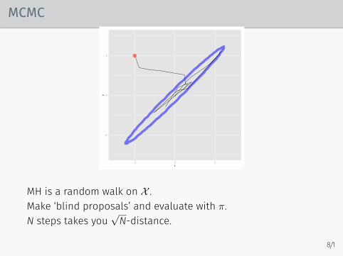
MH is a random walk on X .Make ‘blind proposals’ and evaluate with π.N steps takes you

√N-distance.

8/1

MCMC

−2

0

2

−2 0 2x

y

Gibbs sampler explores X -space one component at a time.

8/1

MCMC

−2

0

2

−2 0 2x

y

Hamiltonian Monte Carlo: Exploit gradient-information aboutπ(x) = f(x)/Z to explore X more efficiently

8/1

Slice samplingUniformly sampling below f(x) gives samples from π(x) ∝ f(x).Slice sampling augments the x with a height y.Runs a Markov chain by updating (x, y).

9/1

Slice sampling

Sample y0 ∼ P(·|x0) = Unif(0, f(x0))

9/1

Slice sampling

9/1

Slice sampling

Given y0, sample

x1 ∼ p(·|y0) = Unif(Ly0),where Lx = {x : f(x) > y0})

Not easy.Make conditional updates: x1 ∼ p(·|x0, y0) 9/1

Slice sampling

Randomly locate a window R around x0; pick x1 ∼ Unif(R ∩ Ly).Observe: if x0 (green), is Unif(y0), then so is x1 (red). Randomlylocating window ensures reversibility.NOT irreducible: can’t jump between modes with long 0-probvalleys

9/1

Slice sampling

Fix: grow window until both ends greater than y0. Different pos-sible strategies. A simple one:• Let current window length be L.• Double the length by adding L/2 segments to random sides.• Repeat till both ends lie above f. 9/1

Slice sampling

Asymmetric growth allows us to reach any mode with nonzeroprobability.

9/1

Slice sampling

Now, uniformly pick points inside window. If point is invalid,truncate window and repeat.

9/1

Slice sampling

When we obtain a valid point, the preceding window can beviewed as a random window with a bunch of auxiliary variables.

9/1

Slice sampling

Note the overall process is reversible

9/1

Date post:	23-Jan-2022
Category:	Documents
Upload:	others
View:	2 times
Download:	0 times

lecture 16: markov chain monte carlo (contd)

Documents