Artificial Neural Network: Deep or Broad? An Empirical Study Nian Liu 1 and Nayyar A. Zaidi 1 Clayton School of Information Technology, Monash University, VIC 3800, Australia {nliu36,nayyar.zaidi}@monash.edu Abstract. Advent of Deep Learning and the emergence of Big Data has led to renewed interests in the study of Artificial Neural Networks (ANN). An ANN is a highly effective classifier that is capable of learning both linear and non-linear boundaries. The number of hidden layers and the number of nodes in each hidden layer (along with many other parameters) in an ANN, is considered to be a model selection problem. With success of deep learning especially on big datasets, there is a prevalent belief in machine learning community that a deep model (that is a model with many number of hidden layers) is preferable. However, this belies earlier theorems proved for ANN that only a single hidden layer (with multiple nodes) is capable of learning any arbitrary function, i.e., a shallow broad ANN. This raises the question of whether one should build a deep network or go for a broad network. In this paper, we do a systematic study of depth and breadth of an ANN in terms of 0-1 Loss, RMSE, Bias, Variance and convergence performance on 72 standard UCI datasets. 1 Introduction The emergence of Big Data and success of deep learning on some problems have sparked a new interest in the study and evaluation of Artificial Neural Networks (ANN). ANN has a long history in the field of Artificial Intelligence. Earliest in- stance of ANN came in the form of Perceptron algorithm [1]. Perceptron was not capable of handling non-linear class boundaries and, therefore, interest in them remained fairly limited. Breakthrough was achieved by the invention of Backprop- agation algorithm and multi-layer Perceptron that could model non-linear bound- aries that led to a golden era of ANN. However, results were not as good as one had expected. Attention of Artificial Intelligence (AI) community was soon diverted to more mathematically sound alternative such as Support Vector Machines (with convex objective function) and non-parametric models such as Decision Trees, Random Forest, etc. With advancements in the computing infrastructure, access to much bigger training datasets and better (for example greedy layer-wised) training algorithms [2] – ANN demonstrated much successes in its application on structured problems 1 1 These are mostly the problems in text, vision and NLP where there is a certain struc- ture present in the input features. For example, deep learning performed extremely well on MNIST digit dataset (accuracy improved over 20%) when compared to typical machine learning algorithms.
Transcript
Artificial Neural Network: Deep or Broad? AnEmpirical Study
Nian Liu1 and Nayyar A. Zaidi1
Clayton School of Information Technology, Monash University, VIC 3800, Australia{nliu36,nayyar.zaidi}@monash.edu
Abstract. Advent of Deep Learning and the emergence of Big Data hasled to renewed interests in the study of Artificial Neural Networks (ANN).An ANN is a highly effective classifier that is capable of learning both linearand non-linear boundaries. The number of hidden layers and the numberof nodes in each hidden layer (along with many other parameters) in anANN, is considered to be a model selection problem. With success of deeplearning especially on big datasets, there is a prevalent belief in machinelearning community that a deep model (that is a model with many numberof hidden layers) is preferable. However, this belies earlier theorems provedfor ANN that only a single hidden layer (with multiple nodes) is capableof learning any arbitrary function, i.e., a shallow broad ANN. This raisesthe question of whether one should build a deep network or go for a broadnetwork. In this paper, we do a systematic study of depth and breadthof an ANN in terms of 0-1 Loss, RMSE, Bias, Variance and convergenceperformance on 72 standard UCI datasets.
1 IntroductionThe emergence of Big Data and success of deep learning on some problems havesparked a new interest in the study and evaluation of Artificial Neural Networks(ANN). ANN has a long history in the field of Artificial Intelligence. Earliest in-stance of ANN came in the form of Perceptron algorithm [1]. Perceptron was notcapable of handling non-linear class boundaries and, therefore, interest in themremained fairly limited. Breakthrough was achieved by the invention of Backprop-agation algorithm and multi-layer Perceptron that could model non-linear bound-aries that led to a golden era of ANN. However, results were not as good as one hadexpected. Attention of Artificial Intelligence (AI) community was soon diverted tomore mathematically sound alternative such as Support Vector Machines (withconvex objective function) and non-parametric models such as Decision Trees,Random Forest, etc.
With advancements in the computing infrastructure, access to much biggertraining datasets and better (for example greedy layer-wised) training algorithms [2]– ANN demonstrated much successes in its application on structured problems1
1 These are mostly the problems in text, vision and NLP where there is a certain struc-ture present in the input features. For example, deep learning performed extremelywell on MNIST digit dataset (accuracy improved over 20%) when compared to typicalmachine learning algorithms.
2 Nian Liu and Nayyar A. Zaidi
and, therefore, there has been a renewed interest in the study of ANN mostlyunder the umbrella term of deep learning. However, applicability of deep learningon problems where there is no structure in the input and studying its efficacy overother competing machine learning algorithms remains to be further investigated.
Deep refers to the fact that the network has to be very deep. Why is deeplearning effective? We believe that this is due to the feature engineering capa-bility of a deep network. For example, for image recognition, lower-level layersrepresent the pixels and middle-levels represent the edges made of these pixelsand higher-levels represent the concepts made from these edges. An example isthe convolutional neural network (CNN), where there is an explicit filtering stage(convolution), followed by max-polling and then a fully-connected network. In anCNN, an image is convolved with a kernel to incorporate the spatial informationpresent in the image, resulting in higher-order features 2. This is followed by somesampling steps, for example, max-pooling to reduce the size of the output. Therecan be many convolution and max-pooling layers, which are followed by a fully-connected multi-layer perceptron. What about problems where we can not relyon interactions in the features? In other words, if we cannot rely on convolutionaland max-pooling layers, will deep learning be as effective as it is on the structuredproblems? Well, we argue, that the success of deep learning can be attributed tothe fact that it takes into account higher-order interactions among the features ofthe data. And when faced with extremely large quantities of training data, takinginto account these higher-order interactions is beneficial [3].
Therefore, for un-structured problems, there are several directions one couldtake of which we mention only three in the following:
1. Take the quadratic, cubic or higher-order features and feed them to an ANNwith no hidden layers [4].
2. Train a multi-layer ANN with many hidden layers – deep model.3. Train an ANN with single hidden layer but many nodes – broad model.
We leave option one as an area of future research, and will focus on the secondand third option.
To the best of our knowledge, there are no comparative studies of deep andbroad ANN in terms of their performance, bias and variance profiles and conver-gence analysis. We claim our main contributions in this paper are:
– We provide a comparison of 0-1 Loss, RMSE, bias and variance of deep ANNs(with two, three, four and five hidden layers) and broad ANNs (with two,four, eight and ten nodes in one hidden layer). We show that on standard UCIdatasets [8], broad ANNs leads to better results than deeper models.
– We compare the convergence analysis of deep ANNs and broad ANNs. We showthat broad ANN have far superior convergence profiles than deeper models.
The rest of this paper is organized as follows. In Section 2, we provide a briefoverview of ANN and learning algorithm used to train the models. In Section 3,
2 Earlier applications of multi-layer perceptrons presented only the pixels to the inputlayer which failed to encode the structure present in the images.
Artificial Neural Network: Deep or Broad? An Empirical Study 3
we provide the empirical results. We conclude in section 4 with pointers to futurework.
2 A Simple Feed-Forward ANN
An Artificial Neural network (ANN) mimics how the neurons in a biological brainwork. In the brain, each neuron receives input from other neurons. The effect andmagnitude of the input is controlled by synaptic weight. The weight will changeover time so that the brain can learn and perform tasks. We will denote the inputlayer of an ANN as X, each hidden layer as Hk, and the output layer will bedenoted as Y . In this paper, we only considered sigmoid nodes with the activationfunction of form: ak = f(hk ·wk), where wk represent the weighting of each layer asmentioned earlier. Also, w0 is the weighting for the input layer. Here, hk representsthe input of each layer and ak represents the output of each layer. Since the outputof the previous layer is the input of the current layer, the following equality holds:
ak−1 = hk (1)
Note that the output of the last hidden layer is input of the output layer. Henceas, where s represents the index of the final hidden layer, will be the predictiongiven by the NN.
The objective function of an ANN is to minimize the Mean Squared Error(MSE) that is:
J(w) =1
2(as − Y )2.
The weights for all layers are randomized initially. Using the input value h0, allactivations functions are calculated layer by layer allowing for an output as. Thisprocess is called forward propagation. Using this output value, back propagationcan be implemented through gradient descent to minimize the MSE.
In order to use gradient descent, we need the partial derivatives of each wk:4wk = δJ
δwk. Let us show the derivation of partial derivatives of the last two layers
and the pattern will be apparent. For the output layer s:
δJ
δws=
δJ
δas
δasδws
.
The first part is the plain derivative of the cost function with respect to as.
δJ
δas= (as − y).
The second part is the derivative of the sigmoid function with respect to ws. Sinceboth hs and ws are variables, chain rule must be used:
δasδws
= f ′(hs · ws)hs.
4 Nian Liu and Nayyar A. Zaidi
Putting it altogether:
4ws = (as − y)f ′(hs · ws)hs = γshs. (2)
Note that we have introduced a new notation of γk. For the second last layer s−1,we have:
δJ
δws−1=
δJ
δas−1
δas−1
δws−1.
Let us focus on the first part:
δJ
δas−1=∑ δ
δas−1
[1
2(as − y)2
].
Note, the above sum is over all the nodes in hidden layer s−1. We have removed thesubscript indexing each node in layer s−1 for simplicity purposes. In the followingequations, all the summations are over the number of nodes in the hidden layerunless explicitly stated otherwise. We expand above Equation as:
δJ
δas−1, =
∑(as − y)
δasδas−1
,
=∑
(as − y)δasδhs
,
=∑
(as − y)f ′(hs · ws)ws =∑
γsws.
The jump from the second line to the third line above is valid because of Equation1. The summation sign is needed because each node in layer s−1 provides an inputto each node in layer s, hence the partial derivatives need to be added together.The second part is the same as before:
δas−1
δws−1= f ′(hs−1 · ws−1)hs−1.
Putting it together:
4ws−1 =∑
γs−1hs−1 =∑
(as − y)f ′(hs · ws)ws × f ′(hs−1 · ws−1)hs−1.
It can be seen that:
γs−1 =∑
γsws · f ′(hs−1 · ws−1).
Using this, we have a general formula for each wk:
4wk−1 =∑
γk−1hk−1 =∑
γkwkf′(hk−1 · wk−1)hk−1,
where γk=s is provided in Equation 2.All the above derivation was for a single class of a single instance. To generalize
it, we only need to sum over all instances and over all classes hence the followingnew cost function – with nc classes and n features, we have:
J(w) =
nc∑ n∑ 1
2(as − y)2.
Artificial Neural Network: Deep or Broad? An Empirical Study 5
Luckily, derivatives of sums are the sum of the derivatives. Hence all the derivationabove is valid in the general case.
4wk−1 =∑
γk−1hk−1 =∑
γkwkf′(hk−1 · wk−1)hk−1,
with
γs =
nc∑ n∑(as − y)f ′(hs · ws).
In this work, we used Stochastic Gradient Descent (SGD) for optimization. Weleave investigation of batch-optimization methods such as quasi-Newton (L-BFGS)and conjugate Gradient methods for future work 3.
3 Experimental Results
In this section, we compare and analyze the performance of our proposed algo-rithms and related methods on 72 natural domains from the UCI repository ofmachine learning datasets [8]. The experiments are conducted on the datasetsdescribed in Table 1. 40 datasets have fewer than 1, 000 instances, 20 datasetshave between 1, 000 and 10, 000 instances and 12 datasets have more than 10, 000instances. These datasets are shown in bold font in Table 1. Each algorithm istested on each dataset using 3 rounds of 2-fold cross validation. We compare fourdifferent metrics, i.e., 0-1 Loss, RMSE, Bias and Variance4. There are a num-ber of different bias-variance decomposition definitions. In this research, we usethe bias and variance definitions of [9] together with the repeated cross-validationbias-variance estimation method proposed by [10]. Kohavi and Wolpert [9] define
bias and variance as follows: bias2 = 12
∑y∈Y
(P(y|x)− P̂(y|x)
)2
, and variance =
12
(1−
∑y∈Y P̂(y|x)2
). We report Win-Draw-Loss (W-D-L) results when compar-
ing the 0-1 Loss, RMSE, bias and variance of two models. A two-tail binomialsign test is used to determine the significance of the results. Results are consideredsignificant if p ≤ 0.05 and shown in bold.
The datasets in Table 1 are divided into three categories. When discussingresults, we denote all the datasets in Table 1 as All. We denote the followingdatasets as Big – Poker-hand, Covertype, Census-income, Localization,
Connect-4, Shuttle, Adult, Letter-recog, Magic, Sign, pendigits. Theremaining datasets (i.e., {All - Big}) are denoted as Little in the results.
Numeric features are discretized by using the Minimum Description Length(MDL) supervised discretization method [11]. A missing value is treated as a sep-arate feature value and taken into account exactly like other values.
3 As the comparison is between a deep and broad model of the same ANN – the exactimplementation of the ANN is less consequential, as long as the implementation isconsistent between the two, we believe that the results should remain valid.
4 The reason for performing bias/variance estimation is that it provides insights intohow the learning algorithm will perform with varying amounts of data. We expect lowvariance algorithms to have relatively low error for small data and low bias algorithmsto have relatively low error for large data [6].
3.1 Comparison in terms of W-D-L and Geometric Averages
Let us start by comparing five broad models with five deep models in terms oftheir Win, Draw and Loss results on standard datasets. We denote broad modelsas NN2, NN4, NN6, NN8 and NN10. This denotes ANN with one hidden layerwith two, four, six, eight and ten nodes in the hidden layer.
We denote deep models as NN2, NN22, NN222, NN2222, NN22222. This de-notes ANN with one hidden layer with two nodes, two hidden layers with twonodes each, three hidden layers with two nodes each, four hidden layers with twonodes each and five hidden layers with two nodes each, respectively.
We also include an ANN with no hidden layer. This is denoted as NN0. Thisis actually similar to Logistic Regression except that it is using Mean-square-errorinstead of Conditional Log-Likelihood (CLL) [4].
Broad Models Let us start with comparing the bias and variance of broad mod-els. We compare the results in Table 2. A systematic trend in bias, as expected canbe seen. A broader model is lower-biased than the less broader model. NN10 beinglowest biased winning significantly in terms of W-D-L when compared to otherlesser broad models. Variance results are slightly surprising. An NN10, though has
Artificial Neural Network: Deep or Broad? An Empirical Study 7
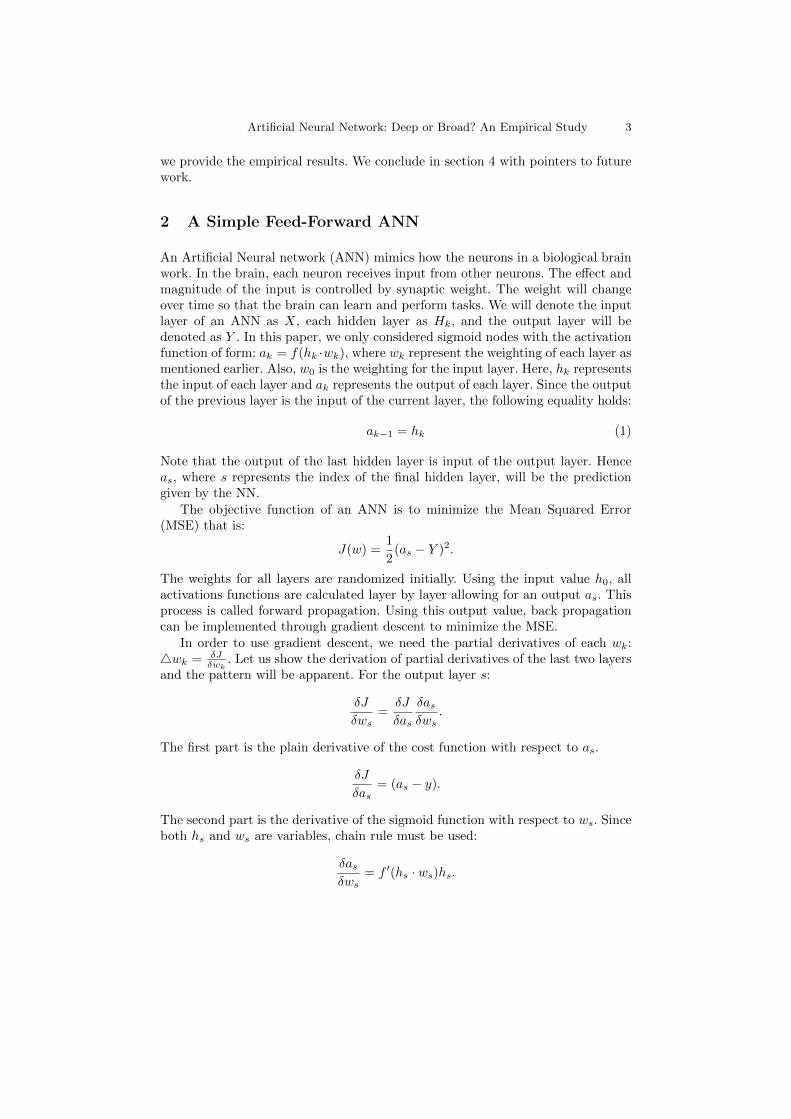
(non-significant) higher variance than NN0, has significantly lower variance thanNN2, NN4 and non-significantly lower variance than NN6 and NN8.
Table 2. A comparison of Bias and Variance of broad models in terms of W-D-L on All datasets. p istwo-tail binomial sign test. Results are significant if p ≤ 0.05.
As discussed in Section 1, lower-bias of broad models translates into better 0-1Loss and RMSE performance on Big datasets. This can be seen in Table 3. It canbe seen that on Big datasets, NN10 leads to much better performance than NN8,NN6, NN4, NN2 and NN0. Some of the results are not significant statistically, buta general trend can be seen that a broader ANN leads to better performance thanless broader ANN.
Table 3. A comparison of 0-1 Loss and RMSE of broad models in terms of W-D-L on All and Bigdatasets. p is two-tail binomial sign test. Results are significant if p ≤ 0.05.
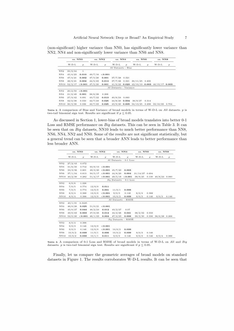
Finally, let us compare the geometric averages of broad models on standarddatasets in Figure 1. The results corroborates W-D-L results. It can be seen that
8 Nian Liu and Nayyar A. Zaidi
All Big0
0.2
0.4
0.6
0.8
1
1.2
1.4
1.6
1.8
20-1 Loss
NN0NN2NN4NN6NN8NN10
All Big0
0.5
1
1.5RMSE
NN0NN2NN4NN6NN8NN10
All Big0
0.5
1
1.5Bias
NN0NN2NN4NN6NN8NN10
All Big0
0.5
1
1.5
2
2.5
3Variance
NN0NN2NN4NN6NN8NN10
Fig. 1. Comparison (geometric average) of 0-1 Loss, RMSE, Bias and Variance for broadmodels on Little and Big datasets. Results are normalized w.r.t NN0.
a broader model leads to a low-biased classifier, which leads to low 0-1 Loss andRMSE. Similarly variance is higher than NN0, but one can not infer a trend inthe growth of variance as model becomes broader and broader.
Deep Models Let us start by comparing the bias-variance profile of deep modelsin Table 4. It can be seen that unlike broad models, a deep model does not leadto low bias at all. In fact, bias increases as the model is made deeper and deeper.It can be seen that only NN2 wins to NN0 (a bare win over one dataset), whereasall other deeper models lose to NN0 in terms of the bias. Similarly, all deepermodels except NN22222 loses significantly to NN0 in terms of variance. N22222(non-significantly) wins to NN0 in terms of the variance.
Table 4. Bias W-D-L on All and Big datasets. p is two-tail binomial sign test. Results are significantif p ≤ 0.05.
A comparison of W-D-L of 0-1 Loss and RMSE values of deep models is givenin Table 5. It can be seen that NN2 and NN22 are competitive with NN0 in termsof RMSE on Big datasets, deeper models NN222, NN2222 and NN22222 are notvery competitive to simple model such as NN0. A comparison of the average 0-1Loss, RMSE, Bias and Variance of different deep models is given in Figure 2. It canbe seen that deeper the model, higher its bias is. The performance in terms of thevariance is very surprising, as it shows that the deep models leads to lower-variancethan simple models such as NN0.
Artificial Neural Network: Deep or Broad? An Empirical Study 9
Table 5. 0-1 Loss W-D-L on All and Big datasets. p is two-tail binomial sign test. Results are significantif p ≤ 0.05.
All Big0
0.5
1
1.5
2
2.5
3
3.5
40-1 Loss
NN0NN2NN22NN222NN2222NN22222
All Big0
0.2
0.4
0.6
0.8
1
1.2
1.4
1.6
1.8
2RMSE
NN0NN2NN22NN222NN2222NN22222
All Big0
0.5
1
1.5
2
2.5
3
3.5
4
4.5
5Bias
NN0NN2NN22NN222NN2222NN22222
All Big0
0.5
1
1.5
2
2.5
3Variance
NN0NN2NN22NN222NN2222NN22222
Fig. 2. Comparison (geometric average) of 0-1 Loss, RMSE, Bias and Variance for deepmodels on Little and Big datasets. Results are normalized w.r.t NN0.
3.2 Deep vs. Broad Models – Discussion
From the comparative results on deep and broad models, one can conclude thatbroader models have better performance than deeper models. However, we stress,that we are comparing very different models in terms of the number of parametersbeing optimized 5, and, hence, we didn’t gave a direct comparison of broad anddeep models. For example, with 10 numeric features and three classes, NN10 willlearn 143, whereas NN22222 will learn 61 parameters. Therefore, we used NN0as the base model against which we compared the performance. We showed that
5 If n is the no. of attributes and nc is the number of classes, then, broad model has((n + 1) ∗N(H1)) + ((N(H1) + 1) ∗ nc) number of parameters, where N(H1) denotesthe number of nodes in hidden layer H1. A deep model, on the other hand, optimizes((n + 1) ∗N(H1)) +
∑Kk=1 (N(Hk) + 1 ∗N(Hk+1)) + ((N(HK) + 1) ∗ nc) number of
parameters.
10 Nian Liu and Nayyar A. Zaidi
100
101
102
103
No. of Iterations
0.01
0.015
0.02
0.025
0.03
0.035
0.04
Me
an
Sq
ua
re
Erro
r
Letter-recog
NN2NN4NN6NN8NN10
100
101
102
103
No. of Iterations
0.095
0.1
0.105
0.11
0.115
0.12
0.125
0.13
0.135
0.14
Me
an
Sq
ua
re
Erro
r
Magic
NN2NN4NN6NN8NN10
100
101
102
103
No. of Iterations
0.09
0.1
0.11
0.12
0.13
0.14
0.15
0.16
0.17
Me
an
Sq
ua
re
Erro
r
Sign
NN2NN4NN6NN8NN10
100
101
102
103
No. of Iterations
0
0.01
0.02
0.03
0.04
0.05
0.06
0.07
0.08
0.09
Me
an
Sq
ua
re
Erro
r
Pendigits
NN2NN4NN6NN8NN10
100
101
102
103
No. of Iterations
0
0.005
0.01
0.015
0.02
0.025
0.03
0.035
0.04
0.045
Me
an
Sq
ua
re
Erro
r
Nursery
NN2NN4NN6NN8NN10
100
101
102
103
No. of Iterations
0.085
0.09
0.095
0.1
0.105
0.11
0.115
0.12
0.125
Me
an
Sq
ua
re
Erro
r
Adult
NN2NN4NN6NN8NN10
100
101
102
103
No. of Iterations
0.036
0.038
0.04
0.042
0.044
0.046
0.048
0.05
0.052
0.054
0.056
Me
an
Sq
ua
re
Erro
r
Census-income
NN2NN4NN6NN8NN10
100
101
102
103
No. of Iterations
0.09
0.095
0.1
0.105
0.11
0.115
0.12
0.125
0.13
0.135
Me
an
Sq
ua
re
Erro
r
Connect-4
NN2NN4NN6NN8NN10
100
101
102
103
No. of Iterations
0.048
0.05
0.052
0.054
0.056
0.058
0.06
0.062
0.064
0.066
Me
an
Sq
ua
re
Erro
r
Localization
NN2NN4NN6NN8NN10
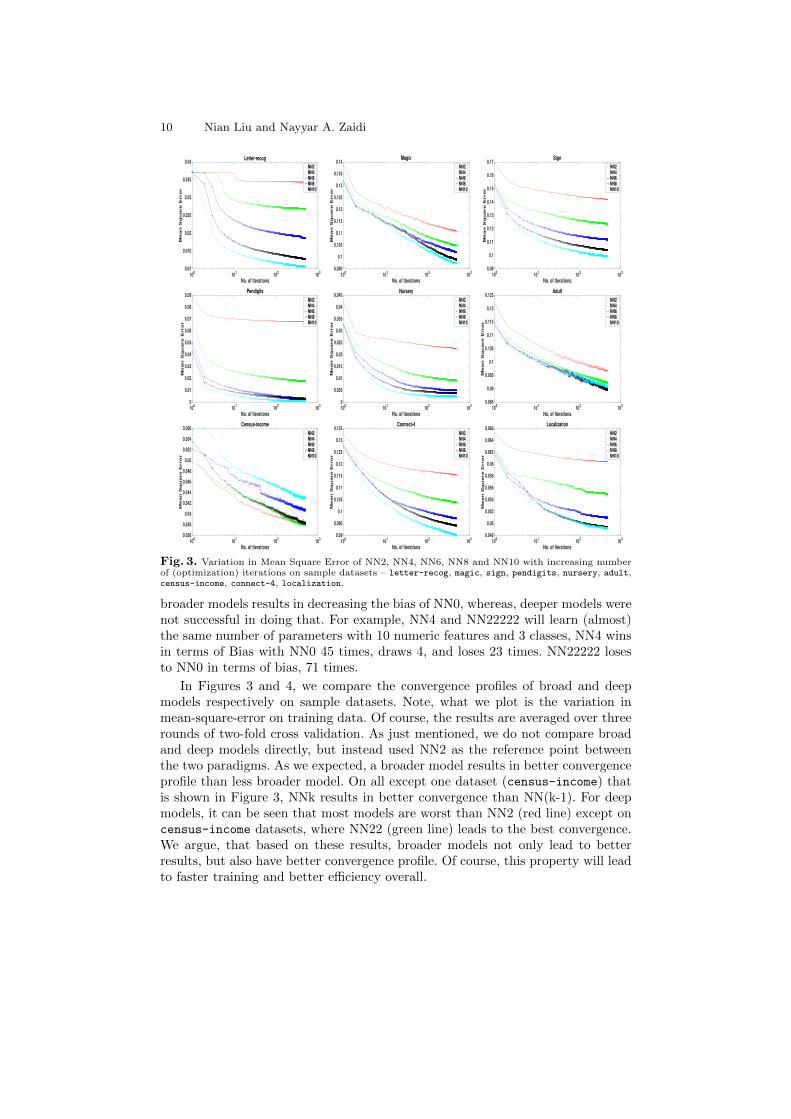
Fig. 3. Variation in Mean Square Error of NN2, NN4, NN6, NN8 and NN10 with increasing numberof (optimization) iterations on sample datasets – letter-recog, magic, sign, pendigits, nursery, adult,census-income, connect-4, localization.
broader models results in decreasing the bias of NN0, whereas, deeper models werenot successful in doing that. For example, NN4 and NN22222 will learn (almost)the same number of parameters with 10 numeric features and 3 classes, NN4 winsin terms of Bias with NN0 45 times, draws 4, and loses 23 times. NN22222 losesto NN0 in terms of bias, 71 times.
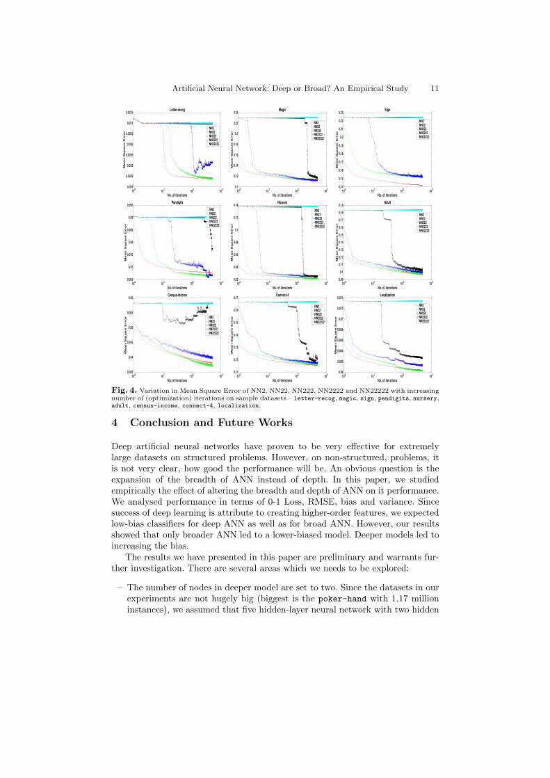
In Figures 3 and 4, we compare the convergence profiles of broad and deepmodels respectively on sample datasets. Note, what we plot is the variation inmean-square-error on training data. Of course, the results are averaged over threerounds of two-fold cross validation. As just mentioned, we do not compare broadand deep models directly, but instead used NN2 as the reference point betweenthe two paradigms. As we expected, a broader model results in better convergenceprofile than less broader model. On all except one dataset (census-income) thatis shown in Figure 3, NNk results in better convergence than NN(k-1). For deepmodels, it can be seen that most models are worst than NN2 (red line) except oncensus-income datasets, where NN22 (green line) leads to the best convergence.We argue, that based on these results, broader models not only lead to betterresults, but also have better convergence profile. Of course, this property will leadto faster training and better efficiency overall.
Artificial Neural Network: Deep or Broad? An Empirical Study 11
100
101
102
103
No. of Iterations
0.034
0.0345
0.035
0.0355
0.036
0.0365
0.037
0.0375
Me
an
Sq
ua
re
Erro
r
Letter-recog
NN2NN22NN222NN2222NN22222
100
101
102
103
No. of Iterations
0.1
0.12
0.14
0.16
0.18
0.2
0.22
0.24
Me
an
Sq
ua
re
Erro
r
Magic
NN2NN22NN222NN2222NN22222
100
101
102
103
No. of Iterations
0.14
0.15
0.16
0.17
0.18
0.19
0.2
0.21
0.22
0.23
Me
an
Sq
ua
re
Erro
r
Sign
NN2NN22NN222NN2222NN22222
100
101
102
103
No. of Iterations
0.065
0.07
0.075
0.08
0.085
0.09
0.095
Me
an
Sq
ua
re
Erro
r
Pendigits
NN2NN22NN222NN2222NN22222
100
101
102
103
No. of Iterations
0.02
0.04
0.06
0.08
0.1
0.12
0.14
Me
an
Sq
ua
re
Erro
r
Nursery
NN2NN22NN222NN2222NN22222
100
101
102
103
No. of Iterations
0.09
0.1
0.11
0.12
0.13
0.14
0.15
0.16
0.17
0.18
0.19
Me
an
Sq
ua
re
Erro
r
Adult
NN2NN22NN222NN2222NN22222
100
101
102
103
No. of Iterations
0.035
0.04
0.045
0.05
0.055
0.06
Me
an
Sq
ua
re
Erro
r
Census-income
NN2NN22NN222NN2222NN22222
100
101
102
103
No. of Iterations
0.11
0.12
0.13
0.14
0.15
0.16
0.17
Me
an
Sq
ua
re
Erro
r
Connect-4
NN2NN22NN222NN2222NN22222
100
101
102
103
No. of Iterations
0.06
0.062
0.064
0.066
0.068
0.07
0.072
0.074
Me
an
Sq
ua
re
Erro
r
Localization
NN2NN22NN222NN2222NN22222
Fig. 4. Variation in Mean Square Error of NN2, NN22, NN222, NN2222 and NN22222 with increasingnumber of (optimization) iterations on sample datasets – letter-recog, magic, sign, pendigits, nursery,adult, census-income, connect-4, localization.
4 Conclusion and Future Works
Deep artificial neural networks have proven to be very effective for extremelylarge datasets on structured problems. However, on non-structured, problems, itis not very clear, how good the performance will be. An obvious question is theexpansion of the breadth of ANN instead of depth. In this paper, we studiedempirically the effect of altering the breadth and depth of ANN on it performance.We analysed performance in terms of 0-1 Loss, RMSE, bias and variance. Sincesuccess of deep learning is attribute to creating higher-order features, we expectedlow-bias classifiers for deep ANN as well as for broad ANN. However, our resultsshowed that only broader ANN led to a lower-biased model. Deeper models led toincreasing the bias.
The results we have presented in this paper are preliminary and warrants fur-ther investigation. There are several areas which we needs to be explored:
– The number of nodes in deeper model are set to two. Since the datasets in ourexperiments are not hugely big (biggest is the poker-hand with 1.17 millioninstances), we assumed that five hidden-layer neural network with two hidden
12 Nian Liu and Nayyar A. Zaidi
nodes in each layer covers the essence of a deep network. Obviously, the numberof nodes in each layer effects the performance and a systematic study is neededto assess the effect on performance.
– The maximum number of optimization iterations are set to 500. It can bethe case that a deeper network just converge slowly, therefore, variations withmore number of iterations needs to be tested.
– In this work, we have constrained ourselves to (feed-forward) multi-layer per-ceptrons – further experimentations needs to be conducted to check if resultswill hold on other ANN types such as Deep Belief Networks or RestrictedBoltzmann machines, etc.
5 Acknowledgment
Authors would like to thank Francois Petitjean, Geoff Webb and Reza Haffari forhelpful discussion during the course of this work. Nian Liu was supported by ECR2015 seed grant by the Faculty of Information Technology, Monash University,Australia.
References
1. F. Rosenblatt, “The perceptron–a perceiving and recognizing automaton,” CornellAeronautical Laboratory, Tech. Rep. 85-460-1, 1957.
2. G. E. Hinton, S. Osindero, and Y. W. Teh, “A fast learning algorithm for deep beliefnets,” Neural Compuation, 2006.
3. X. Zhang and Y. LeCun, “Text understanding from scratch,” arXiv:1502.01710, 2015.4. N. A. Zaidi, F. Petitjean, and G. I. Webb, “Preconditioning an artificial neural net-
work using naive bayes,” in Advances in Knowledge Discovery and Data Mining,2016, pp. 341–353.
5. N. A. Zaidi, G. I. Webb, M. J. Carman, F. Petitjean, and J. Cerquides, “ALRn:Accelerated higher-order logistic regression,” Machine Learning, pp. 1–44, 2016.
6. D. Brain and G. I. Webb, “The need for low bias algorithms in classification learningfrom small data sets,” in PKDD, 2002, pp. 62–73.
7. N. A. Zaidi, M. J. Carman, J. Cerquides, and G. I. Webb, “Naive-Bayes inspiredeffective pre-conditioners for speeding-up logistic regression,” in IEEE InternationalConference on Data Mining, 2014, pp. 1097–1102.
8. A. Frank and A. Asuncion, “UCI machine learning repository,” 2010. [Online].Available: http://archive.ics.uci.edu/ml
9. R. Kohavi and D. Wolpert, “Bias plus variance decomposition for zero-one loss func-tions,” in ICML, 1996, pp. 275–283.
10. G. I. Webb, “Multiboosting: A technique for combining boosting and wagging,”Machine Learning, vol. 40, no. 2, pp. 159–196, 2000.
11. U. M. Fayyad and K. B. Irani, “On the handling of continuous-valued attributes indecision tree generation,” Machine Learning, vol. 8, no. 1, pp. 87–102, 1992.


![Arti cial Intelligence Ph.D. Quali er Study Guide [Rev. 6 ... · Arti cial Intelligence Ph.D. Quali er Study Guide [Rev. 6/18/2014] The Arti cial Intelligence Ph.D. Quali er covers](https://static.documents.pub/doc/80x56/5ceb255c88c9931e1e8dfc4e/arti-cial-intelligence-phd-quali-er-study-guide-rev-6-arti-cial-intelligence.jpg)


