221
Krzysztof Patan Artificial Neural Networks for the Modelling and Fault Diagnosis of Technical Processes ABC

Krzysztof Patan
Artificial Neural Networks forthe Modelling and FaultDiagnosis of TechnicalProcesses
ABC

Series Advisory BoardF. Allgöwer, P. Fleming, P. Kokotovic,A.B. Kurzhanski, H. Kwakernaak,A. Rantzer, J.N. Tsitsiklis
AuthorKrzysztof PatanUniversity of Zielona GóraInst. Control andComputation Engineeringul. Podgórna 5065-246 Zielona GóraPolandE-Mail: [email protected]
ISBN 978-3-540-79871-2 e-ISBN 978-3-540-79872-9
DOI 10.1007/978-3-540-79872-9
Lecture Notes in Control and Information Sciences ISSN 0170-8643
Library of Congress Control Number: 2008926085
c© 2008 Springer-Verlag Berlin Heidelberg
This work is subject to copyright. All rights are reserved, whether the whole or part of the material isconcerned, specifically the rights of translation, reprinting, reuse of illustrations, recitation, broadcasting,reproduction on microfilm or in any other way, and storage in data banks. Duplication of this publication orparts thereof is permitted only under the provisions of the German Copyright Law of September 9, 1965, inits current version, and permission for use must always be obtained from Springer. Violations are liable forprosecution under the German Copyright Law.
The use of general descriptive names, registered names, trademarks, etc. in this publication does not imply,even in the absence of a specific statement, that such names are exempt from the relevant protective laws andregulations and therefore free for general use.
Typeset & Cover Design: Scientific Publishing Services Pvt. Ltd., Chennai, India.
Printed in acid-free paper
5 4 3 2 1 0
springer.com

To my beloved wife Agnieszka,and children Weronika and Leonard,
for their patience and tolerance

Foreword
An unappealing characteristic of all real-world systems is the fact that they arevulnerable to faults, malfunctions and, more generally, unexpected modes of be-haviour. This explains why there is a continuous need for reliable and universalmonitoring systems based on suitable and effective fault diagnosis strategies.This is especially true for engineering systems, whose complexity is permanentlygrowing due to the inevitable development of modern industry as well as theinformation and communication technology revolution. Indeed, the design andoperation of engineering systems require an increased attention with respect toavailability, reliability, safety and fault tolerance. Thus, it is natural that faultdiagnosis plays a fundamental role in modern control theory and practice. Thisis reflected in plenty of papers on fault diagnosis in many control-oriented con-ferences and journals. Indeed, a large amount of knowledge on model based faultdiagnosis has been accumulated through scientific literature since the beginningof the 1970s. As a result, a wide spectrum of fault diagnosis techniques havebeen developed.
A major category of fault diagnosis techniques is the model based one, wherean analytical model of the plant to be monitored is assumed to be available.Unfortunately, a fundamental difficulty related to the model based approach isthe fact that there are always modelling uncertainties due to unmodelled dis-turbances, simplifications, idealisations, linearisations, model parameter inaccu-racies and so on. Another important difficulty concerns the intrinsic non-linearcharacteristic of most engineering systems. Indeed, with a few exceptions, mostof the well-established approaches presented in the literature can be applied tolinear systems only. This fact, of course, considerably limits their application inmodern industrial control systems.
Therefore, it is clear that there is a need for both modelling and fault diag-nosis techniques for non-linear dynamic systems, which must ensure robustnessto modelling uncertainties. Presently, many researchers see artificial neural net-works as a strong alternative to the classical methods used in the model basedfault diagnosis framework. Indeed, due to their interesting properties as func-tional approximators, neural networks turn out to be a very promising tool for

VIII Foreword
dealing with non-linear processes. Although a considerable research attentionhas been drawn to the application of neural networks in this important researcharea, the existing publications on the specific class of locally recurrent neuralnetworks considered in this book are rather scarse. To date, very few workscan be found in the literature presenting locally recurrent neural networks in aunified framework including stability analysis, approximation abilities, trainingsequences selection as well as industrial applications.
The book presents the application of neural networks to the modelling andfault diagnosis of industrial processes. The first two chapters focus on the funda-mental issues such as the basic definitions and fault diagnosis schemes as well asa survey on ways of using neural networks in different fault diagnosis strategies.This part is of a tutorial value and can be perceived as a good starting point forthe newcomers to this field. Chapter 3 presents a special class of locally recurrentneural networks, addressing their properties and training algorithms. Investiga-tions regarding stability, approximation capabilities and the selection of optimalinput training sequences are carried out in the subsequent three chapters. Chap-ter 7 describes decision making methods including robustness analysis. The lastchapter shows original achievements in the area of fault diagnosis of industrialprocesses. All the concepts described in this book are illustrated with eithersimple academic examples or real-world practical applications.
Because of the fact that both theory and practical applications are discussed,the book is expected to be useful for both academic researchers and professionalengineers working in industry. The first group may be especially interested inthe fundamental issues and/or some inspirations regarding future research di-rections concerning fault diagnosis. The second group may be interested in prac-tical implementations which can be very helpful in industrial applications of thetechniques described in this publication. Thus, the book can be strongly recom-mended to both researchers and practitioners in the wide field of fault detection,supervision and safety of technical processes.
February, 2008 Prof. Thomas ParisiniUniversity of Trieste, Italy

Preface
It is well understood that fault diagnosis has become an important issue inmodern automatic control theory. Early diagnosis of faults that might occurin the supervised process renders it possible to perform important preventingactions. Moreover, it allows one to avoid heavy economic losses involved instopped production, the replacement of elements and parts. The core of faultdiagnosis methodology is the so-called model based scheme, where either ana-lytical or knowledge based models are used in combination with decision makingprocedures.
The fundamental idea of model based fault diagnosis is to generate signalsthat reflect inconsistencies between nominal and faulty system operating condi-tions. In the case of complex systems, however, one is faced with the problemthat no accurate or no sufficiently accurate mathematical models are available.A solution of the problem can be obtained through the use of artificial neuralnetworks. For the last two and a half decades there has been observed significantdevelopment in the so-called dynamic neural networks. One of the most inter-esting solutions of the dynamic system identification problem is the applicationof locally recurrent globally feedforward networks.
The book is mainly focused on investigating the properties of locally recurrentneural networks, developing training procedures for them and their applicationto the modelling and fault diagnosis of non-linear dynamic processes and plants.
The material included in the monograph results from research that has beencarried out at the Institute of Control and Computation Engineering of theUniversity of Zielona Gora, Poland, for the last eight years in the area of themodelling of non-linear dynamic processes as well as fault diagnosis of industrialprocesses. Some of the presented results were developed with the support of theMinistry of Science and Higher Education in Poland under the grants Artificialneural networks in robust diagnostic systems (2007-2008) and Modelling andidentification of non-linear dynamic systems in robust diagnostics (2004-2007).The work was also supported by the EC under the RTN project Developmentand Application of Methods for Actuator Diagnosis in Industrial Control SystemsDAMADICS (2000-2004).

X Preface
The monograph is divided into nine chapters. The first chapter constitutesan introduction to the theory of the modelling and fault diagnosis of technicalprocesses. Chapter 2 focuses on the modelling issue in fault diagnosis, especiallyon the model based scheme and neural networks’ role in it. Chapter 3 deals witha special class of locally recurrent neural networks, investigating its propertiesand training algorithms. The next three chapters discuss the fundamental issuesof locally recurrent networks, namely approximation abilities, stability and sta-bilization procedures, and selecting optimal input training sequences. Chapter7 discusses several methods of decision making in the context of fault diagno-sis including both constant and adaptive thresholds. Finally, Chapter 9 showsoriginal achievements in the area of fault diagnosis of industrial processes.
At this point, I would like to express my sincere thanks to Prof. Jozef Korbiczfor suggesting the problem, his invaluable help and continuous support. Theauthor is grateful to all the friends at the Institute of Control and ComputationEngineering of the University of Zielona Gora for many stimulating discussionsand friendly atmosphere required for finishing this work. Especially, I wouldlike to thank my brother Maciek for his partial contribution to Chapter 6, andWojtek Paszke for support in the area of linear matrix inequalities. Finally, Iwould like to express my gratitude to Ms Agnieszka Rozewska for proofreadingand linguistic advise on the text.
Zielona Gora, Krzysztof PatanFebruary, 2008
Contents
1 Introduction . . . . . . . . . . . . . . . . . . . . . . . . . . . . . . . . . . . . . . . . . . . . . . . . 11.1 Organization of the Book . . . . . . . . . . . . . . . . . . . . . . . . . . . . . . . . . . 3
2 Modelling Issue in Fault Diagnosis . . . . . . . . . . . . . . . . . . . . . . . . . . 72.1 Problem of Fault Detection and Fault Diagnosis . . . . . . . . . . . . . . 82.2 Models Used in Fault Diagnosis . . . . . . . . . . . . . . . . . . . . . . . . . . . . 11
2.2.1 Parameter Estimation . . . . . . . . . . . . . . . . . . . . . . . . . . . . . . . 122.2.2 Parity Relations . . . . . . . . . . . . . . . . . . . . . . . . . . . . . . . . . . . . 122.2.3 Observers . . . . . . . . . . . . . . . . . . . . . . . . . . . . . . . . . . . . . . . . . 132.2.4 Neural Networks . . . . . . . . . . . . . . . . . . . . . . . . . . . . . . . . . . . 142.2.5 Fuzzy Logic . . . . . . . . . . . . . . . . . . . . . . . . . . . . . . . . . . . . . . . 15
2.3 Neural Networks in Fault Diagnosis . . . . . . . . . . . . . . . . . . . . . . . . . 162.3.1 Multi-layer Feedforward Networks . . . . . . . . . . . . . . . . . . . . 162.3.2 Radial Basis Function Network . . . . . . . . . . . . . . . . . . . . . . . 182.3.3 Kohonen Network . . . . . . . . . . . . . . . . . . . . . . . . . . . . . . . . . . 202.3.4 Model Based Approaches . . . . . . . . . . . . . . . . . . . . . . . . . . . . 212.3.5 Knowledge Based Approaches . . . . . . . . . . . . . . . . . . . . . . . . 232.3.6 Data Analysis Approaches . . . . . . . . . . . . . . . . . . . . . . . . . . . 23
2.4 Evaluation of the FDI System . . . . . . . . . . . . . . . . . . . . . . . . . . . . . . 242.5 Summary . . . . . . . . . . . . . . . . . . . . . . . . . . . . . . . . . . . . . . . . . . . . . . . . 26
3 Locally Recurrent Neural Networks . . . . . . . . . . . . . . . . . . . . . . . . 293.1 Neural Networks with External Dynamics . . . . . . . . . . . . . . . . . . . 303.2 Fully Recurrent Networks . . . . . . . . . . . . . . . . . . . . . . . . . . . . . . . . . 313.3 Partially Recurrent Networks . . . . . . . . . . . . . . . . . . . . . . . . . . . . . . 323.4 State-Space Networks . . . . . . . . . . . . . . . . . . . . . . . . . . . . . . . . . . . . . 343.5 Locally Recurrent Networks . . . . . . . . . . . . . . . . . . . . . . . . . . . . . . . . 36
3.5.1 Model with the IIR Filter . . . . . . . . . . . . . . . . . . . . . . . . . . . 403.5.2 Analysis of Equilibrium Points . . . . . . . . . . . . . . . . . . . . . . . 433.5.3 Controllability and Observability . . . . . . . . . . . . . . . . . . . . . 473.5.4 Dynamic Neural Network . . . . . . . . . . . . . . . . . . . . . . . . . . . . 49
3.6 Training of the Network . . . . . . . . . . . . . . . . . . . . . . . . . . . . . . . . . . . 52

XII Contents
3.6.1 Extended Dynamic Back-Propagation . . . . . . . . . . . . . . . . . 523.6.2 Adaptive Random Search . . . . . . . . . . . . . . . . . . . . . . . . . . . . 533.6.3 Simultaneous Perturbation Stochastic Approximation . . . 553.6.4 Comparison of Training Algorithms . . . . . . . . . . . . . . . . . . . 57
3.7 Summary . . . . . . . . . . . . . . . . . . . . . . . . . . . . . . . . . . . . . . . . . . . . . . . . 62
4 Approximation Abilities of Locally Recurrent Networks . . . . 654.1 Modelling Properties of the Dynamic Neuron . . . . . . . . . . . . . . . . 66
4.1.1 State-Space Representation of the Network . . . . . . . . . . . . 674.2 Preliminaries . . . . . . . . . . . . . . . . . . . . . . . . . . . . . . . . . . . . . . . . . . . . . 674.3 Approximation Abilities . . . . . . . . . . . . . . . . . . . . . . . . . . . . . . . . . . . 684.4 Process Modelling . . . . . . . . . . . . . . . . . . . . . . . . . . . . . . . . . . . . . . . . 724.5 Summary . . . . . . . . . . . . . . . . . . . . . . . . . . . . . . . . . . . . . . . . . . . . . . . . 74
5 Stability and Stabilization of Locally Recurrent Networks . . 775.1 Stability Analysis – Networks with One Hidden Layer . . . . . . . . . 78
5.1.1 Gradient Projection . . . . . . . . . . . . . . . . . . . . . . . . . . . . . . . . 825.1.2 Minimum Distance Projection . . . . . . . . . . . . . . . . . . . . . . . 825.1.3 Strong Convergence . . . . . . . . . . . . . . . . . . . . . . . . . . . . . . . . 865.1.4 Numerical Complexity . . . . . . . . . . . . . . . . . . . . . . . . . . . . . . 885.1.5 Pole Placement . . . . . . . . . . . . . . . . . . . . . . . . . . . . . . . . . . . . 905.1.6 System Identification Based on Real Process Data . . . . . . 925.1.7 Convergence of Network States . . . . . . . . . . . . . . . . . . . . . . . 93
5.2 Stability Analysis – Networks with Two Hidden Layers . . . . . . . . 965.2.1 Second Method of Lyapunov . . . . . . . . . . . . . . . . . . . . . . . . . 975.2.2 First Method of Lyapunov . . . . . . . . . . . . . . . . . . . . . . . . . . . 105
5.3 Stability Analysis – Cascade Networks . . . . . . . . . . . . . . . . . . . . . . 1105.4 Summary . . . . . . . . . . . . . . . . . . . . . . . . . . . . . . . . . . . . . . . . . . . . . . . . 111
6 Optimum Experimental Design for Locally RecurrentNetworks . . . . . . . . . . . . . . . . . . . . . . . . . . . . . . . . . . . . . . . . . . . . . . . . . . . 1136.1 Optimal Sequence Selection Problem in Question . . . . . . . . . . . . . 114
6.1.1 Statistical Model . . . . . . . . . . . . . . . . . . . . . . . . . . . . . . . . . . . 1146.1.2 Sequence Quality Measure . . . . . . . . . . . . . . . . . . . . . . . . . . . 1156.1.3 Experimental Design . . . . . . . . . . . . . . . . . . . . . . . . . . . . . . . . 116
6.2 Characterization of Optimal Solutions . . . . . . . . . . . . . . . . . . . . . . . 1176.3 Selection of Training Sequences . . . . . . . . . . . . . . . . . . . . . . . . . . . . 1186.4 Illustrative Example . . . . . . . . . . . . . . . . . . . . . . . . . . . . . . . . . . . . . . 119
6.4.1 Simulation Setting . . . . . . . . . . . . . . . . . . . . . . . . . . . . . . . . . . 1196.4.2 Results . . . . . . . . . . . . . . . . . . . . . . . . . . . . . . . . . . . . . . . . . . . . 120
6.5 Summary . . . . . . . . . . . . . . . . . . . . . . . . . . . . . . . . . . . . . . . . . . . . . . . . 121
7 Decision Making in Fault Detection . . . . . . . . . . . . . . . . . . . . . . . . . 1237.1 Simple Thresholding . . . . . . . . . . . . . . . . . . . . . . . . . . . . . . . . . . . . . . 1247.2 Density Estimation . . . . . . . . . . . . . . . . . . . . . . . . . . . . . . . . . . . . . . . 126
7.2.1 Normality Testing . . . . . . . . . . . . . . . . . . . . . . . . . . . . . . . . . . 126

Contents XIII
7.2.2 Density Estimation . . . . . . . . . . . . . . . . . . . . . . . . . . . . . . . . . 1277.2.3 Threshold Calculating – A Single Neuron . . . . . . . . . . . . . . 1307.2.4 Threshold Calculating – A Two-Layer Network . . . . . . . . . 131
7.3 Robust Fault Diagnosis . . . . . . . . . . . . . . . . . . . . . . . . . . . . . . . . . . . 1327.3.1 Adaptive Thresholds . . . . . . . . . . . . . . . . . . . . . . . . . . . . . . . . 1337.3.2 Fuzzy Threshold Adaptation . . . . . . . . . . . . . . . . . . . . . . . . . 1357.3.3 Model Error Modelling . . . . . . . . . . . . . . . . . . . . . . . . . . . . . . 137
7.4 Summary . . . . . . . . . . . . . . . . . . . . . . . . . . . . . . . . . . . . . . . . . . . . . . . . 140
8 Industrial Applications . . . . . . . . . . . . . . . . . . . . . . . . . . . . . . . . . . . . . 1418.1 Sugar Factory Fault Diagnosis . . . . . . . . . . . . . . . . . . . . . . . . . . . . . 141
8.1.1 Instrumentation Faults . . . . . . . . . . . . . . . . . . . . . . . . . . . . . . 1438.1.2 Actuator Faults . . . . . . . . . . . . . . . . . . . . . . . . . . . . . . . . . . . . 1438.1.3 Experiments . . . . . . . . . . . . . . . . . . . . . . . . . . . . . . . . . . . . . . . 1468.1.4 Final Remarks . . . . . . . . . . . . . . . . . . . . . . . . . . . . . . . . . . . . . 160
8.2 Fluid Catalytic Cracking Fault Detection . . . . . . . . . . . . . . . . . . . . 1618.2.1 Process Modelling . . . . . . . . . . . . . . . . . . . . . . . . . . . . . . . . . . 1638.2.2 Faulty Scenarios . . . . . . . . . . . . . . . . . . . . . . . . . . . . . . . . . . . . 1648.2.3 Fault Diagnosis . . . . . . . . . . . . . . . . . . . . . . . . . . . . . . . . . . . . 1648.2.4 Robust Fault Diagnosis . . . . . . . . . . . . . . . . . . . . . . . . . . . . . 1688.2.5 Final Remarks . . . . . . . . . . . . . . . . . . . . . . . . . . . . . . . . . . . . . 172
8.3 DC Motor Fault Diagnosis . . . . . . . . . . . . . . . . . . . . . . . . . . . . . . . . . 1728.3.1 AMIRA DR300 Laboratory System . . . . . . . . . . . . . . . . . . . 1738.3.2 Motor Modelling . . . . . . . . . . . . . . . . . . . . . . . . . . . . . . . . . . . 1768.3.3 Fault Diagnosis Using Density Shaping . . . . . . . . . . . . . . . . 1768.3.4 Robust Fault Diagnosis . . . . . . . . . . . . . . . . . . . . . . . . . . . . . 1818.3.5 Final Remarks . . . . . . . . . . . . . . . . . . . . . . . . . . . . . . . . . . . . . 182
9 Concluding Remarks and Further Research Directions . . . . . . 187
References . . . . . . . . . . . . . . . . . . . . . . . . . . . . . . . . . . . . . . . . . . . . . . . . . . . . . . 191
Index . . . . . . . . . . . . . . . . . . . . . . . . . . . . . . . . . . . . . . . . . . . . . . . . . . . . . . . . . . . 203

List of Figures
2.1 Scheme of the diagnosed automatic control system . . . . . . . . . . . . . 82.2 Types of faults: abrupt (dashed), incipient (solid) and
intermittent (dash-dot) . . . . . . . . . . . . . . . . . . . . . . . . . . . . . . . . . . . . . 92.3 Two stages of fault diagnosis . . . . . . . . . . . . . . . . . . . . . . . . . . . . . . . . 102.4 General scheme of model based fault diagnosis . . . . . . . . . . . . . . . . 112.5 Neuron scheme with n inputs and one output . . . . . . . . . . . . . . . . . 172.6 Three layer perceptron with n inputs and m outputs . . . . . . . . . . . 182.7 Structure of the radial basis function network with n inputs
and m outputs . . . . . . . . . . . . . . . . . . . . . . . . . . . . . . . . . . . . . . . . . . . . 192.8 Model based fault diagnosis using neural networks . . . . . . . . . . . . . 222.9 Model-free fault diagnosis using neural networks . . . . . . . . . . . . . . . 242.10 Fault diagnosis as pattern recognition . . . . . . . . . . . . . . . . . . . . . . . . 252.11 Definition of the benchmark zone . . . . . . . . . . . . . . . . . . . . . . . . . . . . 25
3.1 External dynamics approach realization . . . . . . . . . . . . . . . . . . . . . . 303.2 Fully recurrent network of Williams and Zipser . . . . . . . . . . . . . . . . 323.3 Partialy recurrent networks due to Elman (a) and Jordan (b) . . . 333.4 Architecture of the recurrent multi-layer perceptron . . . . . . . . . . . 343.5 Block scheme of the state-space neural network with one
hidden layer . . . . . . . . . . . . . . . . . . . . . . . . . . . . . . . . . . . . . . . . . . . . . . 343.6 Generalized structure of the dynamic neuron unit (a), network
composed of dynamic neural units (b) . . . . . . . . . . . . . . . . . . . . . . . . 363.7 Neuron architecture with local activation feedback . . . . . . . . . . . . . 393.8 Neuron architecture with local synapse feedback . . . . . . . . . . . . . . . 393.9 Neuron architecture with local output feedback . . . . . . . . . . . . . . . 403.10 Memory neuron architecture . . . . . . . . . . . . . . . . . . . . . . . . . . . . . . . . 413.11 Neuron architecture with the IIR filter . . . . . . . . . . . . . . . . . . . . . . . 413.12 Transformation of the neuron model with the IIR filter to the
general local activation feedback structure . . . . . . . . . . . . . . . . . . . . 423.13 State-space form of the i-th neuron with the IIR filter . . . . . . . . . . 43

XVI List of Figures
3.14 Positions of equilibrium points: stable node (a), stable focus(b), unstable node (c), unstable focus (d), saddle point (e),center (f) . . . . . . . . . . . . . . . . . . . . . . . . . . . . . . . . . . . . . . . . . . . . . . . . . 44
3.15 Eigenvalue positions of the matrix A: γ = 0.3 (a), γ = 0.5 (b) . . . 453.16 Eigenvalue positions of the modified matrix A: γ = 0.3 (a),
γ = 0.5 (b) . . . . . . . . . . . . . . . . . . . . . . . . . . . . . . . . . . . . . . . . . . . . . . . 463.17 Topology of the locally recurrent globally feedforward
network . . . . . . . . . . . . . . . . . . . . . . . . . . . . . . . . . . . . . . . . . . . . . . . . . . 503.18 Learning error for different algorithms . . . . . . . . . . . . . . . . . . . . . . . 603.19 Testing phase: EDBP (a), ARS (b) and SPSA (c). Actuator
(black), neural model (grey). . . . . . . . . . . . . . . . . . . . . . . . . . . . . . . . . 61
4.1 i-th neuron of the second layer . . . . . . . . . . . . . . . . . . . . . . . . . . . . . . 704.2 Cascade structure of the modified dynamic neural network . . . . . . 704.3 Cascade structure of the modified dynamic neural network . . . . . . 72
5.1 Result of the experiment – an unstable system . . . . . . . . . . . . . . . . 805.2 Result of the experiment – a stable system . . . . . . . . . . . . . . . . . . . 815.3 Idea of the gradient projection . . . . . . . . . . . . . . . . . . . . . . . . . . . . . . 835.4 Stability triangle and the search region . . . . . . . . . . . . . . . . . . . . . . . 845.5 Sum squared error – training without stabilization . . . . . . . . . . . . . 905.6 Poles location during learning without stabilization: neuron 1
(a), neuron 2 (b), neuron 3 (c), neuron 4 (d) . . . . . . . . . . . . . . . . . . 915.7 Poles location during learning, stabilization using GP: neuron
1 (a), neuron 2 (b), neuron 3 (c), neuron 4 (d) . . . . . . . . . . . . . . . . 925.8 Poles location during learning without stabilization: neuron 1
(a), neuron 2 (b), neuron 3 (c), neuron 4 (d) . . . . . . . . . . . . . . . . . . 935.9 Poles location during learning, stabilization using MDP:
neuron 1 (a), neuron 2 (b), neuron 3 (c), neuron 4 (d) . . . . . . . . . . 945.10 Actuator (solid line) and model (dashed line) outputs for
learning (a) and testing (b) data sets . . . . . . . . . . . . . . . . . . . . . . . . 945.11 Results of training without stabilization: error curve (a) and
the convergence of the state x(k) of the neural model (b) . . . . . . . 955.12 Results of training with GP: error curve (a) and the
convergence of the state x(k) of the neural model (b) . . . . . . . . . . 955.13 Results of training with MDP: error curve (a) and the
convergence of the state x(k) of the neural model (b) . . . . . . . . . . 965.14 Convergence of network states: original system (a)–(b),
transformed system (c)–(d), learning track (e) . . . . . . . . . . . . . . . . . 995.15 Convergence of network states: original system (a)–(b),
transformed system (c)–(d), learning track (e) . . . . . . . . . . . . . . . . . 1025.16 Graphical solution of the problems (5.70) . . . . . . . . . . . . . . . . . . . . . 109
6.1 Convergence of the design algorithm . . . . . . . . . . . . . . . . . . . . . . . . . 1206.2 Average variance of the model response prediction for optimum
design (diamonds) and random design (circles) . . . . . . . . . . . . . . . . 121

List of Figures XVII
7.1 Residual with thresholds calculated using: (7.3) (a), (7.5) withζ = 1 (b), (7.5) with ζ = 2 (c), (7.5) with ζ = 3 (d) . . . . . . . . . . . . 125
7.2 Normality testing: comparison of cumulative distributionfunctions (a), probability plot (b) . . . . . . . . . . . . . . . . . . . . . . . . . . . 127
7.3 Neural network for density calculation . . . . . . . . . . . . . . . . . . . . . . . 1297.4 Simple two-layer network . . . . . . . . . . . . . . . . . . . . . . . . . . . . . . . . . . . 1297.5 Output of the network (7.20) with the threshold (7.34) . . . . . . . . . 1317.6 Residual signal (solid), adaptive thresholds calculated using
(7.38) (dotted), and adaptive thresholds calculated using(7.39) (dashed) . . . . . . . . . . . . . . . . . . . . . . . . . . . . . . . . . . . . . . . . . . . . 135
7.7 Illustration of the fuzzy threshold adaptation . . . . . . . . . . . . . . . . . 1367.8 Scheme of the fault detection system with the threshold
adaptation . . . . . . . . . . . . . . . . . . . . . . . . . . . . . . . . . . . . . . . . . . . . . . . 1377.9 Idea of the fuzzy threshold . . . . . . . . . . . . . . . . . . . . . . . . . . . . . . . . . 1377.10 Model error modelling: error model training (a), confidence
region constructing (b) . . . . . . . . . . . . . . . . . . . . . . . . . . . . . . . . . . . . . 1387.11 Idea of model error modelling: system output (solid), centre of
the uncertainty region (dotted), confidence bands (dashed) . . . . . 139
8.1 Evaporation station. Four heaters and the first evaporationsection . . . . . . . . . . . . . . . . . . . . . . . . . . . . . . . . . . . . . . . . . . . . . . . . . . . 142
8.2 Actuator to be diagnosed (a), block scheme of theactuator (b) . . . . . . . . . . . . . . . . . . . . . . . . . . . . . . . . . . . . . . . . . . . . . . 144
8.3 Causal graph of the main actuator variables . . . . . . . . . . . . . . . . . . 1458.4 Residual signal for the vapour model in different faulty
situations: fault in P51 03 (900–1200), fault in T 51 07(1800–2100) . . . . . . . . . . . . . . . . . . . . . . . . . . . . . . . . . . . . . . . . . . . . . . 148
8.5 Residual signals for the temperature model in different faultysituations: fault in F51 01 (0–300), fault in F51 02 (325–605),fault in T 51 06 (1500-1800), fault in T 51 08 (2100–2400), faultin TC51 05 (2450–2750) . . . . . . . . . . . . . . . . . . . . . . . . . . . . . . . . . . . . 149
8.6 Normal operating conditions: residual with the constant (a)and the adaptive (b) threshold . . . . . . . . . . . . . . . . . . . . . . . . . . . . . . 151
8.7 Residual for different faulty situations . . . . . . . . . . . . . . . . . . . . . . . . 1528.8 Residual of the nominal model (output F ) in the case of the
faults f1 (a), f2 (b) and f3 (c) . . . . . . . . . . . . . . . . . . . . . . . . . . . . . . 1548.9 Residual of the nominal model (output X) in the case of the
faults f1 (a), f2 (b) and f3 (c) . . . . . . . . . . . . . . . . . . . . . . . . . . . . . . 1558.10 Residuals of the fault models f1 (a) and (d); f2 (b) and (e); f3
(c) and (f) in the case of the fault f1 . . . . . . . . . . . . . . . . . . . . . . . . . 1568.11 Residuals of the fault models f1 (a) and (d); f2 (b) and (e); f3
(c) and (f) in the case of the fault f2 . . . . . . . . . . . . . . . . . . . . . . . . . 1578.12 Residuals of the fault models f1 (a) and (d); f2 (b) and (e); f3
(c) and (f) in the case of the fault f3 . . . . . . . . . . . . . . . . . . . . . . . . . 1588.13 General scheme of the fluid catalytic cracking converter . . . . . . . . 162

XVIII List of Figures
8.14 Results of modelling the temperature of the cracking mixture(8.9) . . . . . . . . . . . . . . . . . . . . . . . . . . . . . . . . . . . . . . . . . . . . . . . . . . . . . 163
8.15 Residual signal . . . . . . . . . . . . . . . . . . . . . . . . . . . . . . . . . . . . . . . . . . . . 1648.16 Cumulative distribution functions: normal – solid,
residual – dashed . . . . . . . . . . . . . . . . . . . . . . . . . . . . . . . . . . . . . . . . . . 1658.17 Probability plot for the residual . . . . . . . . . . . . . . . . . . . . . . . . . . . . . 1658.18 Residual histogram (a), network output histogram (b),
estimated PDF and the confidence interval (c) . . . . . . . . . . . . . . . . 1668.19 Residual histogram (a), network output histogram (b),
estimated PDF and the confidence interval (c) . . . . . . . . . . . . . . . . 1678.20 Residual (solid) and the error model output (dashed) under
nominal operating conditions . . . . . . . . . . . . . . . . . . . . . . . . . . . . . . . 1698.21 Confidence bands and the system output under nominal
operating conditions . . . . . . . . . . . . . . . . . . . . . . . . . . . . . . . . . . . . . . . 1708.22 Residual with constant thresholds under nominal operating
conditions . . . . . . . . . . . . . . . . . . . . . . . . . . . . . . . . . . . . . . . . . . . . . . . . 1708.23 Fault detection results: scenario f1 (a), scenario f2 (b),
scenario f3 (c) . . . . . . . . . . . . . . . . . . . . . . . . . . . . . . . . . . . . . . . . . . . . 1718.24 Laboratory system with a DC motor . . . . . . . . . . . . . . . . . . . . . . . . . 1748.25 Equivalent electrical circuit of a DC motor . . . . . . . . . . . . . . . . . . . 1768.26 Responses of the motor (solid) and the neural model
(dash-dot) – open-loop control . . . . . . . . . . . . . . . . . . . . . . . . . . . . . . 1778.27 Responses of the motor (solid) and the neural model
(dashed) – closed-loop control . . . . . . . . . . . . . . . . . . . . . . . . . . . . . . . 1778.28 Symptom distribution . . . . . . . . . . . . . . . . . . . . . . . . . . . . . . . . . . . . . . 1798.29 Residual and constant thresholds (a) and confidence bands
generated by model error modelling (b) . . . . . . . . . . . . . . . . . . . . . . 1828.30 Fault detection using model error modelling: fault f1
1 –confidence bands (a) and decision logic without the timewindow (b); fault f1
6 – confidence bands (c) and decision logicwithout the time window (d); fault f2
4 – confidence bands (e)and decision logic without the time window (f) . . . . . . . . . . . . . . . . 183
8.31 Fault detection by using constant thresholds: fault f11 –
residual with thresholds (a) and decision logic without thetime window (b); fault f1
6 – residual with thresholds (c) anddecision logic without the time window (d); fault f2
4 – residualwith thresholds (e) and decision logic without the timewindow (f) . . . . . . . . . . . . . . . . . . . . . . . . . . . . . . . . . . . . . . . . . . . . . . . 184
List of Tables
3.1 Specification of different types of dynamic neuron units . . . . . . . . 383.2 Outline of ARS . . . . . . . . . . . . . . . . . . . . . . . . . . . . . . . . . . . . . . . . . . . 553.3 Outline of the basic SPSA . . . . . . . . . . . . . . . . . . . . . . . . . . . . . . . . . . 573.4 Characteristics of learning methods . . . . . . . . . . . . . . . . . . . . . . . . . . 593.5 Characteristics of learning methods . . . . . . . . . . . . . . . . . . . . . . . . . . 62
4.1 Selection results of the cascade dynamic neural network . . . . . . . . 734.2 Selection results of the two-layer dynamic neural network . . . . . . . 73
5.1 Outline of the gradient projection . . . . . . . . . . . . . . . . . . . . . . . . . . . 835.2 Outline of the minimum distance projection . . . . . . . . . . . . . . . . . . 865.3 Number of operations: GP method . . . . . . . . . . . . . . . . . . . . . . . . . . 895.4 Number of operations: MDP method . . . . . . . . . . . . . . . . . . . . . . . . . 895.5 Comparison of the learning time for different methods . . . . . . . . . 905.6 Outline of norm stability checking . . . . . . . . . . . . . . . . . . . . . . . . . . . 1005.7 Comparison of methods . . . . . . . . . . . . . . . . . . . . . . . . . . . . . . . . . . . . 1055.8 Outline of constrained optimisation training . . . . . . . . . . . . . . . . . . 110
6.1 Sample mean and the standard deviation of parameterestimates . . . . . . . . . . . . . . . . . . . . . . . . . . . . . . . . . . . . . . . . . . . . . . . . . 120
7.1 Threshold calculating . . . . . . . . . . . . . . . . . . . . . . . . . . . . . . . . . . . . . . 132
8.1 Specification of process variables . . . . . . . . . . . . . . . . . . . . . . . . . . . . 1438.2 Description of symbols . . . . . . . . . . . . . . . . . . . . . . . . . . . . . . . . . . . . . 1448.3 Selection of the neural network for the vapour model . . . . . . . . . . . 1488.4 Number of false alarms . . . . . . . . . . . . . . . . . . . . . . . . . . . . . . . . . . . . . 1508.5 Neural models for nominal conditions and faulty scenarios . . . . . . 1538.6 Results of fault detection (a) and isolation (b)
(X – detectable/isolable, N – not detectable/notisolable) . . . . . . . . . . . . . . . . . . . . . . . . . . . . . . . . . . . . . . . . . . . . . . . . . . 159
8.7 Modelling quality for different models . . . . . . . . . . . . . . . . . . . . . . . . 159

XX List of Tables
8.8 FDI properties of the examined approaches . . . . . . . . . . . . . . . . . . . 1608.9 Specification of measurable process variables . . . . . . . . . . . . . . . . . . 1638.10 Comparison of false detection rates . . . . . . . . . . . . . . . . . . . . . . . . . . 1688.11 Performance indices for faulty scenarios . . . . . . . . . . . . . . . . . . . . . . 1688.12 Performance indices for faulty scenarios . . . . . . . . . . . . . . . . . . . . . . 1698.13 Laboratory system technical data . . . . . . . . . . . . . . . . . . . . . . . . . . . . 1758.14 Results of fault detection for the density shaping technique . . . . . 1788.15 Fault isolation results . . . . . . . . . . . . . . . . . . . . . . . . . . . . . . . . . . . . . . 1808.16 Fault identification results . . . . . . . . . . . . . . . . . . . . . . . . . . . . . . . . . . 1818.17 Results of fault detection for model error modelling . . . . . . . . . . . . 185

Nomenclature
Symbols
R set of real numberst, k continuous and discrete-time indexesx(·) state vectoru(·) input vectory(·) output vectorσ(·) activation functionσ(·) vector-valued activation functionA state matrixW weight matrixC output matrixB feed-forward filter parameters matrixD transfer matrixG slope parameters matrixg vector of biasesθ, θ vector of network parameters and its estimateN (m, v) normally distributed random number with the expectation
value m and the standard deviation vβ significance levelC1 class of continuously differentiable mappingsI identity matrix0 zero matrixC set of constraintsK set of violated constraintsA− pseudo-inverse of a matrix Artd, rfd true and false detection rates, respectivelyrti, rfi true and false isolation rates, respectivelytdt time of fault detection

XXII List of Tables
Operators
P probabilityE expectationE[·|·] conditional expectationsup least upper bound (supremum)inf greatest lower bound (infimum)max maximummin minimumrank(A) rank of a matrix Adet(A) determinant of a matrix Atrace(A) trace of a matrix A
Abbrevations
FDI Fault Detection and IsolationUIO Unknown Input ObserverGMDH Group Method and Data HandlingBP Back-PropagationRBF Radial Basis FunctionRTRN Real-Time Recurrent NetworkRMLP Recurrent Multi-Layer PerceptronIIR Infinite Impulse ResponseFIR Finite Impulse ResponseLRGF Locally Recurrent Globally Feed-forwardARS Adaptive Random SearchEDBP Extended Dynamic Back-PropagationSPSA Simultaneous Perturbation Stochastic ApproximationBIBO Bounded Input Bounded OutputGP Gradient ProjectionMDP Minimum Distance ProjectionODE Ordinary Differential Equationsw.p.1 with probability 1a.s. almost surelyLMI Linear Matrix InequalityOED Optimum Experimental DesignARX Auto-Regressive with eXogenous inputNNARX Neural Network Auto-Regressive with eXogenous inputMEM Model Error ModellingSCADA Supervisory Control And Data AcquisitionAIC Akaike Information CriterionFPE Final Prediction ErrorMIMO Multi Input Multi OutputMISO Multi Input Single OutputFCC Fluid Catalytic CrackingDC Direct Current
1 Introduction
The diagnostics of industrial processes is a scientific discipline aimed at thedetection of faults in industrial plants, their isolation, and finally their identifi-cation. Its main task is the diagnosis of process anomalies and faults in processcomponents, sensors and actuators. Early diagnosis of faults that might occur inthe supervised process renders it possible to perform important preventing ac-tions. Moreover, it allows one to avoid heavy economic losses involved in stoppedproduction, the replacement of elements and parts, etc.
Most of the methods in the fault diagnosis literature are based on linearmethodology or exact models. Industrial processes are often difficult to model.They are complex and not exactly known, measurements are corrupted by noiseand unreliable sensors. Therefore, a number of researchers have perceived artifi-cial neural networks as an alternative way to represent knowledge about faults[1, 2, 3, 4, 5, 6, 7]. Neural networks can filter out noise and disturbances, theycan provide stable, highly sensitive and economic diagnostics of faults withouttraditional types of models. Another desirable feature of neural networks is thatno exact models are required to reach the decision stage [2]. In a typical opera-tion, the process model may be only approximate and the critical measurementsmay be able to map internally the functional relationships that represent theprocess, filter out the noise, and handle correlations as well. Although there aremany promising simulation examples of neural networks in fault diagnosis inthe literature, real applications are still quite rare. There is a great necessityto conduct more detailed scientific investigations concerning the application ofneural networks in real industrial plants, to achieve complete utilization of theirattractive features.
One of the most frequently used schemes for fault diagnosis is the modelbased concept. The basic idea of model based fault diagnosis is to generatesignals that reflect inconsistencies between nominal and faulty system operationconditions [8, 9, 10, 11]. Such signals, called residuals, are usually calculated byusing analytical methods such as observers [9, 12], parameter estimation methods[13, 14] or parity equations [15, 16]. Unfortunately, the common drawback ofthese approaches is that an accurate mathematical model of the diagnosed plant
K. Patan: Artificial. Neural Net. for the Model. & Fault Diagnosis, LNCIS 377, pp. 1–6, 2008.springerlink.com c© Springer-Verlag Berlin Heidelberg 2008
2 1 Introduction
is required. When there are no mathematical models of the diagnosed systemor the complexity of a dynamic system increases and the task of modelling isvery hard to implement, analytical models cannot be applied or cannot givesatisfactory results. In these cases data based models, such as neural networks,fuzzy sets or their combination (neuro-fuzzy networks), can be considered.
In recent years, a great deal of attention has been paid to the application of ar-tificial neural networks in the modelling and identification of dynamic processes[17, 18, 19, 20], adaptive control systems [19, 21, 22], time series prediction prob-lems [23, 24]. A growing interest in the application of artificial neural networks tofault diagnosis systems has also been observed [25, 26, 7, 6, 4, 27]. Artificial neu-ral networks provide an excellent mathematical tool for dealing with non-linearproblems. They have an important property according to which any continuousnon-linear relationship can be approximated with arbitrary accuracy using a neu-ral network with a suitable architecture and weight parameters [23, 28]. Theiranother attractive property is the self learning ability. A neural network canextract the system features from historical training data using the learning algo-rithm, requiring little or no a priori knowledge about the process. This providesthe modelling of non-linear systems with a great flexibility [19, 23, 29]. Thesefeatures allow one to design adaptive control systems for complex, unknown andnon-linear dynamic processes. As opposed to many effective applications, e.g. inpattern recognition problems [30, 31], the approximation of non-linear functions[32, 33], the application of neural networks in control systems requires taking intoconsideration the dynamics of the processes being investigated. The applicationof feedforward neural networks with the back-propagation learning algorithm incontrol systems requires the introduction of delay elements [7, 18, 19, 34, 21].Such a solution is needed because these relatively simple and easy to applynetworks are of a static type [19, 29]. Hence, their application possibilities inrelation to dynamic problems are very limited and insufficient. Recurrent neuralnetworks are characterized by considerably better properties, assessing from thepoint of view of their application in control theory [35, 36, 37]. Due to feedbacksintroduced to the network architecture it is possible to accumulate historical dataand use them later. Feed-back can be either local or global. Globally recurrentnetworks can model a wide class of dynamic processes; however, they possessdisadvantages such as slow convergence of learning and stability problems [18].In general, these architectures seem to be too complex for practical implementa-tions. Furthermore, the fixed relationship between the number of states and thenumber of neurons does not allow adjusting the dynamics of the model and itsnon-linear behaviour separately. The drawbacks of globally recurrent networkscan be partly avoided by using locally recurrent networks [38, 26, 39]. Such net-works have a feedforward multi-layer architecture and their dynamic propertiesare obtained using a specific kind of neuron models [38, 40].
One of the possible solutions is the use of neuron models with the InfiniteImpulse Response (IIR) filter. Due to introducing a linear dynamic system intothe neuron structure, the neuron activation depends on its current inputs aswell as past inputs and outputs. The conditions for global stability of the neural
1.1 Organization of the Book 3
network considered can be derived using pole placement and the Lyapunov sec-ond method. Neural networks with two hidden layers possess much more power-ful properties than networks with one hidden layer. Therefore, the stabilizationof such networks is a problem of crucial importance. The issue of calculatingbounds on the network parameters based on the elaborated stability conditionsin order to guarantee that the final neural model after training is stable is alsoa challenging objective.
Most studies on locally recurrent globally feedforward networks are focusedon training algorithms and stability problems. Literature about approximationabilities of such networks is rather scarce. An interesting topic is dealing withinvestigating approximation abilities of a locally recurrent neural network. Thedifferent structures of dynamic networks can be analysed to answer the ques-tion of how many layers are necessary to approximate a state-space trajectoryproduced by any continuous function with arbitrary accuracy. It is also fascinat-ing to investigate how these results can be used in a broader sense in order toestimate a number of neurons needed to ensure a given level of approximationaccuracy.
Another important issue is the problem of how to select the training data tocarry out the training as effectively as possible. The theory related to OptimalExperimental Design (OED) can be applied here. The problem can be stated asfollows: where to locate measurement sensors so as to guarantee the maximalaccuracy of parameter estimation. This is of paramount interest in applications,as it is generally impossible to measure the system state over the entire do-main. The optimal measurement problem is very attractive from the viewpointof the degree of optimality and it does arise in a variety of applications. At themoment there is no contribution of experimental design for dynamic neural net-works to the existing state-of-the-art. Therefore, this topic seems to be the mostchallenging one.
Dynamic neural networks can be successfully applied to design model basedfault diagnosis. However, model based fault diagnosis is founded on a number ofidealized assumptions. One of them is that the model of the system is a faithfulreplica of plant dynamics. Another one is that disturbances and noise acting uponthe system are known. This is, of course, not possible in engineering practice.The robustness problem in fault diagnosis can be defined as the maximisationof the detectability and isolability of faults and simultaneously the minimisationof uncontrolled effects such as disturbances, noise, changes in inputs and/orthe state, etc. Therefore, the problem of estimating model uncertainty is ofparamount importance taking into account the number of false alarms appearingin the monitoring system.
1.1 Organization of the Book
The remaining part of the book consists of the following chapters:
Modelling issue in fault diagnosis. The chapter is divided into four parts.The objective of the first part (Section 2.1) is to introduce the reader into

4 1 Introduction
the theory of fault detection and diagnosis. This part explains the main tasksthat fault diagnosis system should provide, defines fault types and phasesof the diagnostic procedure. Section 2.2 presents the most popular methodsused in model based fault diagnosis. This section discusses parameter esti-mation methods, parity relations, observers, neural networks and fuzzy logicmodels. The main advantages and drawbacks of the discussed techniques areportrayed. A brief introduction to popular structures of neural networks isgiven in Section 2.3. This section also presents three main classes of fault di-agnosis methods, i.e. model based, knowledge based and data analysis basedapproaches with emphasis put on neural networks’ role in these schemes. Inorder to validate a diagnostic procedure, a number of performance indicesare introduced in Section 2.4.
Locally recurrent neural networks. The first part of the chapter, consitingof Sections 3.1, 3.2, 3.3 and 3.4, deals with network structures in which dy-namics are realized using time delays and global feedbacks. The well knownstructures are discussed, i.e. the Williams-Zipser structure, partially recur-rent networks, state-space models, with a rigorous analysis of their advan-tages and shortcomings. Section 3.5 presents locally recurrent structures,with the main emphasis on networks designed with neuron models with theIIR filter. This part of the chapter consists of original research results in-cluding the analysis of equilibrium points of the neuron, its observability andcontrolability. Training methods intended for use with locally recurrent net-works are described in Section 3.6. Three algorithms are presented: extendeddynamic back-propagation, adaptive random search and simultaneous per-turbation stochastic approximation [6, 41, 26, 42, 43, 44, 45].
Approximation abilities of locally recurrent networks. The chapter con-tains original research which deals with investigating approximation abilitiesof a special class of discrete-time locally recurrent neural networks [46, 47].The chapter includes analytical results showing that a locally recurrent net-work with two hidden layers is able to approximate a state-space trajec-tory produced by any Lipschitz continuous function with arbitrary accuracy[46, 47]. Moreover, based on these results, the network can be simplified andtransformed into a more practical structure needed in real world applica-tions. In Section 4.1, modelling properties of a single dynamic neuron arepresented. The dynamic neural network and its representation in the state-space are described in Section 4.1.1. Some preliminaries required to showapproximation abilities of the proposed network are discussed in Section4.2. The main result concerning the approximation of state-space trajecto-ries is presented in Section 4.3 [46, 47]. Section 4.4 illustrates the identifi-cation of a real technological process using the locally recurrent networksconsidered [46].
Stability and stabilization of locally recurrent networks. The chapterpresents originally developed algorithms for stability analysis and the sta-bilization of a class of discrete-time locally recurrent neural networks [45,48, 49]. In Section 5.1, stability issues of the dynamic neural network with

1.1 Organization of the Book 5
one hidden layer are discussed. The training of the network under an ac-tive set of constraints is formulated (Sections 5.1.1 and 5.1.2) [45] togetherwith convergence analysis of the proposed projection algorithms (Section5.1.3) [49]. The section reports also experimental results including complex-ity analysis (Section 5.1.4) and stabilization effectiveness of the proposedmethods (Section 5.1.5) as well as their application to the identification ofan industrial process (Section 5.1.6). Section 5.2 presents stability analysisbased on Lyapunov’s methods [48]. Theorems based on the second methodof Lyapunov are presented in Section 5.2.1. In turn, algorithms utilizing Lya-punov’s first method are discussed in Section 5.2.2. Section 5.3 is devotedto stability analysis of the cascade locally recurrent network proposed inChapter 4.
Optimal experiment design for locally recurrent networks. Original de-velopments about input data selection for the training process of a locallyrecurrent neural network are presented. At the moment there is no contri-bution of optimal selection of input sequences for locally recurrent neuralnetworks to the existing state-of-the-art in the area. Therefore, this topicseems to be the most challenging one among these proposed in the mono-graph. The chapter aims to fill this gap and propose a practical approachfor input data selection for the training process of the locally recurrent neu-ral network. The first part of the chapter, including Sections 6.1 and 6.2,gives the fundamental knowledge about optimal experimental design. Theproposed solution of selecting training sequences is formulated in Section6.3. Section 6.4 contains results of a numerical experiment showing the per-formance of the delineated approach.
Decision making in fault detection. The chapter discusses several methodsof decision making in the context of fault diagnosis. It is composed of twoparts. The first part, consisting of Sections 7.1 and 7.2, is devoted to algo-rithms and methods of constant thresholds calculation. Section 7.1 brieflydescribes known algorithms for generating simple thresholds based on theassumption that a residual signal has a normal distribution. A sligthly dif-ferent original approach is shown in Section 7.2, where first a simple neuralnetwork is used to approximate the probability density function of a residual,and then a threshold is calculated [50, 51, 52]. The second part, includingSection 7.3, presents several robust techniques for decision making. Section7.3.1 discusses a statistical approach to adapt the threshold using the timewindow and recalculating the mean value and the standard deviation ofa residual [53]. The application of fuzzy logic to threshold adaptation isdescribed in Section 7.3.2 [54]. The original solution to design the robustdecision making process obtained through model error modelling and neuralnetworks is investigated in Section 7.3.3 [55, 56].
Industrial applications. The chapter presents original achievements in thearea of fault diagnosis of industrial processes. Section 8.1 includes experi-mental results of fault detection and isolation of selected parts of the sugar

6 1 Introduction
evaporator [26, 49, 44, 45, 43, 42, 57, 54, 58, 59]. The experiments presentedin this section were carried out using real process data. Section 8.2 consistsof results concerning fault detection of selected components of the fluid cat-alytic cracking process [52, 50, 55]. The experiments presented in this sectionwere carried out using simulated data. The last example, fault detection,isolation and identification of the electrical motor, is shown in Section 8.3[51, 56]. The experiments presented in this section were carried out usingreal process data.

2 Modelling Issue in Fault Diagnosis
When introducing fault diagnosis as a scientific discipline, it is worth providingsome basic definitions. These definitions, suggested by the IFAC Technical Com-mittee SAFEPROCESS, have been introduced in order to unify the terminologyin the area.
Fault is an unpermitted deviation of at least one characteristic property orvariable of the system from acceptable/usual/standard behaviour.
Failure is a permanent interruption of the system ability to perform a requiredfunction under specified operating conditions.
Fault detection is a determination of faults present in the system and the timeof detection.
Fault isolation is a determination of the kind, location, and time of detectionof a fault. Follows fault detection.
Fault identification is a determination of the size and time-variant behaviourof a fault. Follows fault isolation.
Fault diagnosis is a determination of the kind, size, location and time of de-tection of a fault. Follows fault detection. Includes both fault isolation andfault identification.
In the literature, there exist also other definitions of fault diagnosis. A verypopular definition of fault diagnosis includes also fault detection [60]. Such adefinition of fault diagnosis is used in this monograph.
The chapter is divided into four main parts. Section 2.1 is an introductionto fault diagnosis theory. This section explains the main objectives of fault di-agnosis, defines fault types and phases of the diagnostic procedure. Section 2.2presents the most popular methods used for model based fault diagnosis. Thissection discusses parameter estimation methods, parity relations, observers, neu-ral networks and fuzzy logic models. The main advantages and drawbacks of thediscussed techniques are portrayed. A brief introduction to popular structuresof neural networks is given in Section 2.3. The section presents also three mainclasses of fault diagnosis methods, i.e. model based, knowledge based and data
K. Patan: Artificial. Neural Net. for the Model. & Fault Diagnosis, LNCIS 377, pp. 7–27, 2008.springerlink.com c© Springer-Verlag Berlin Heidelberg 2008
8 2 Modelling Issue in Fault Diagnosis
analysis based approaches, with emphasis put on neural networks’ role in theseschemes. Each diagnostic algorithm should be validated to confirm its effective-ness and usefulness for real-world fault diagnosis. Some indices needed for thispurpose are introduced in Section 2.4. The chapter concludes with some finalremarks in Section 2.5.
2.1 Problem of Fault Detection and Fault Diagnosis
The main objective of the fault diagnosis system is to determine the location andoccurrence time of possible faults based on accessible data and knowledge aboutthe behaviour of the diagnosed process, e.g. using mathematical, quantitative orqualitative models. Advanced methods of supervision and fault diagnosis shouldsatisfy the following requirements [13]:
• early detection of small faults, abrupt as well as incipient,• diagnosis of faults in actuators, process components or sensors,• detection of faults in closed loop control,• supervision of processes in transient states.
The aim of early detection and diagnosis is to have enough time to take coun-teractions such as reconfiguration, maintenance, repair or other operations.
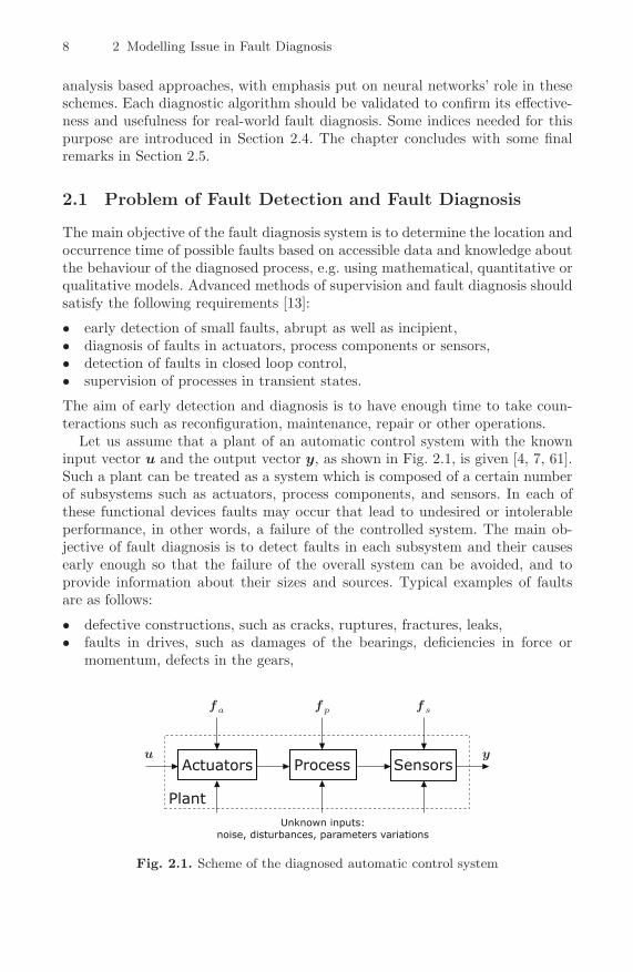
Let us assume that a plant of an automatic control system with the knowninput vector u and the output vector y, as shown in Fig. 2.1, is given [4, 7, 61].Such a plant can be treated as a system which is composed of a certain numberof subsystems such as actuators, process components, and sensors. In each ofthese functional devices faults may occur that lead to undesired or intolerableperformance, in other words, a failure of the controlled system. The main ob-jective of fault diagnosis is to detect faults in each subsystem and their causesearly enough so that the failure of the overall system can be avoided, and toprovide information about their sizes and sources. Typical examples of faultsare as follows:
• defective constructions, such as cracks, ruptures, fractures, leaks,• faults in drives, such as damages of the bearings, deficiencies in force or
momentum, defects in the gears,
fa f p f s
u yActuators
Plant
Unknown inputs:
noise, disturbances, parameters variations
Process Sensors
Fig. 2.1. Scheme of the diagnosed automatic control system
2.1 Problem of Fault Detection and Fault Diagnosis 9
• faults in sensors – scaling errors, hysteresis, drift, dead zones, shortcuts,• abnormal parameter variations,• external obstacles – collisions, the clogging of outflows.
Taking into account the scheme shown in Fig. 2.1, it is useful to divide faultsinto three categories: actuator (final control element), component and sensorfaults, respectively. Actuator faults fa can be viewed as any malfunction of theequipment that actuates the system, e.g. a malfunction of the pneumatic servo-motor in the control valve in the evaporation station [7, 26]. Component faults(process faults) fp occur when some changes in the system make the dynamicrelation invalid, e.g. a leakage in a gas pipeline [62]. Sensor faults fs can beviewed as serious measurements variations. Faults can commonly be describedas inputs. In addition, there is always modelling uncertainty due to unmodelleddisturbances, noise and the model (see Fig. 2.1). This may not be critical to theprocess behaviour, but may obscure fault detection by rising false alarms.
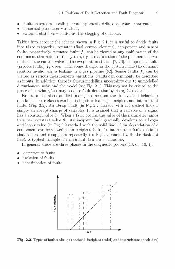
Faults can be also classified taking into account the time-variant behaviourof a fault. Three classes can be distinguished: abrupt, incipient and intermittentfaults (Fig. 2.2). An abrupt fault (in Fig 2.2 marked with the dashed line) issimply an abrupt change of variables. It is asumed that a variable or a signalhas a constant value θ0. When a fault occurs, the value of the parameter jumpsto a new constant value θ1. An incipient fault gradually develops to a largerand larger value (in Fig 2.2 marked with the solid line). Slow degradation of acomponent can be viewed as an incipient fault. An intermittent fault is a faultthat occurs and disappears repeatedly (in Fig 2.2 marked with the dash-dotline). A typical example of such a fault is a loose connector.
In general, there are three phases in the diagnostic process [13, 63, 10, 7]:
• detection of faults,• isolation of faults,• identification of faults.
Fig. 2.2. Types of faults: abrupt (dashed), incipient (solid) and intermittent (dash-dot)

10 2 Modelling Issue in Fault Diagnosis
The main objective of fault detection is to make a decision whether a fault hasoccurred or not. Fault isolation should give information about fault location,which requires that faults be distinguishable. Finally, fault identification com-prises the determination of the size of a fault and the time of its occurrence.In practice, however, the identification phase appears rarely and sometimes itis incorporated into fault isolation. Thus, from the practical point of view, thediagnostic process consists of two phases only: fault detection and isolation.Therefore, the common abbreviation used in many papers is FDI (Fault Detec-tion and Isolation). In other words, automatic fault diagnosis can be viewed as asequential process involving symptom extraction and the actual diagnostic task.Usually, a complete fault diagnosis system consists of two parts (Fig. 2.3):
• residual generation,• residual evaluation.
The residual generation process is based on a comparison between the measuredand predicted system outputs. As a result, the difference or the so-called resid-ual is expected to be near zero under normal operating conditions, but on theoccurrence of a fault a deviation from zero should appear. In turn, the residualevaluation module is dedicated to the analysis of the residual signal in order todetermine whether a fault has occurred and to isolate the fault in a particularsystem device.
Fault detection can be performed either with or without the use of a pro-cess model. In the first case, the detection phase includes generating residualsusing models (analytical, neural, rough, fuzzy, etc.) and estimating residual val-ues. It consists in transforming quantitative diagnostic residuals into qualitativeones and making a decision about the identification of symptoms. In the lattercase, methods of limit value checking or the checking of simple relations betweenprocess variables are used in order to obtain special features of the diagnosedprocess. This process is often called feature extraction or diagnostic signal gener-ation. These features are then compared with the normal features of the healthy
Faults f Disturbances d
PROCESS
Residual generation
Residual evaluation
Input u(k) Output y(k)
Residuals r
Faults f
Fig. 2.3. Two stages of fault diagnosis

2.2 Models Used in Fault Diagnosis 11
Faults
PLANT
Nominal
model
Residual generation Residual evaluation
Fault
classifierFaultmodel1
Faultmodel n
�
�
�
u k( ) y k( )
y k0( ) r0
r1
rn
y k1( )
y kn( )
f
+
+
+
-
-
-
Fig. 2.4. General scheme of model based fault diagnosis
process. To carry out this process, change detection and classification methodscan be applied.
One of the most well-known approaches to residual generation is the modelbased concept. In the general case, this concept can be realized using differentkinds of models: analytical, knowledge based and data based ones [64]. Unfor-tunately, the analytical model based approach is usually restricted to simplersystems described by linear models. When there are no mathematical models ofthe diagnosed system or the complexity of a dynamic system increases and thetask of modelling is very hard to achieve, analytical models cannot be applied orcannot give satisfactory results. In these cases data based models, such as neuralnetworks, fuzzy sets or their combination (neuro-fuzzy networks), can be consid-ered. Figure 2.4 illustrates how the fault diagnosis system can be designed usingmodels of the system. As can be seen in Fig. 2.4, a bank of process models shouldbe designed. Each model represents one class of the system behaviour. One modelrepresents the system under its normal operating conditions and each successiveone – a faulty situation [7]. After that, the residuals can be determined by com-paring the system output y(k) and the ouputs of models y0(k), y1(k),...,yn(k).In this way, the residual vector r = [r0, r1, . . . , rn], which characterizes a suit-able class of the system behaviour, can be obtained. Finally, the residual vectorr should be transformed by a classifier to determine the location and time offault occurrence. It is worth noting here that it is impossible to model all poten-tial system faults. The designer of FDI systems can construct models based onavailable data. In many cases, however, only data for normal operating condi-tions are available and data for faulty scenarios have to be simulated. Therefore,when designing faulty models using, e.g. neural networks, serious problems canbe encountered.
2.2 Models Used in Fault Diagnosis
The section presents models most frequently used in the framework of modelbased fault diagnosis. Due to the comprehensive and vast literature available at

12 2 Modelling Issue in Fault Diagnosis
the moment, the presented models are discussed very briefly. A more completedescription of many models used in fault diagnosis can be found in [65, 13, 4,15, 9, 14, 7, 25, 12].
2.2.1 Parameter Estimation
In most practical cases, the process parameters are not known at all or are notknown exactly enough. Then they can be determined by parameter estimationmethods if the basic structure of the model is known by measuring input andoutput signals. Consider the process described by
y(k) = ΨT θ, (2.1)
where Ψ is the regressor vector, Ψ = [−y(k − 1), . . . , −y(k − m), u(k), . . . , u(k −n)]T , and θ is the parameter vector, θ = [a1, ..., am, b0, ..., bn]T . Assuming thatthe parameter vector θ has physical meaning, the task consists in detecting faultsin a system by measuring the input u(k) and the output y(k), and then givingthe estimate of the parameters of the system model θ. If the fault is modelledas an additive term f acting on the parameter vector of the system
θ = θnom + f , (2.2)
where θnom represents the nominal (fault-free) parameter vector, then the pa-rameter estimate θ indicates a change in the parameters as follows:
Δθ = θ − θ. (2.3)
Fault detection decision making leads to checking if the norm of the parame-ters change (2.3) is greater than a predefined threshold value. The methods ofthreshold determining are widely presented in Chapter 7. Therefore, the problemimplies on-line parameter estimation, which can be solved with various recur-sive algorithms, such as the recursive least-square method [66], the instrumentalvariable approach [67] or the bounded-error approach [68]. The main drawbackof this approach is that the model parameters should have physical meaning, i.e.they should correspond to the parameters of the system. In such situations, thedetection and isolation of faults is very straightforward. If this is not the case, itis usually difficult to distinguish a fault from a change in the parameter vectorθ resulting from time-varying properties of the system. Moreover, the process offault isolation may become extremely difficult because the model parameters donot uniquely correspond to those of the system. It should also be pointed outthat the detection of faults in sensors and actuators is possible but rather com-plicated [14]. Parameter estimation can also be applied to non-linear processes[69, 70, 66].
2.2.2 Parity Relations
Consider a linear process described by the following transfer function:
GP (s) =BP (s)AP (s)
. (2.4)

2.2 Models Used in Fault Diagnosis 13
If the structure of the process as well as the parameters are known, the processmodel is represented by
GM (s) =BM (s)AM (s)
. (2.5)
Assume that fu(t) and fy(t) are additive faults acting on the input and output,respectively. If GP (s) = GM (s), the output error has the form
e′(s) = y(s) − GMu(s) = GP (s)fu(s) + fy(s). (2.6)
Faults that influence the input or output of the process result in changes of theresidual e′(t) with different transients. The polynomials of GM (s) can also beused to form a polynomial error :
e(s) = AM (s)y(s) − BM (s)u(s) = Ap(s)fy(s) + Bp(s)fu(s). (2.7)
Equations (2.6) and (2.7) are known as parity equations (parity relations) [15].Parity relations can also be derived from the state-space representation; thenthey offer more freedom in the design of parity relations [16].
The fault isolation strategy can be relatively easily realised for sensor faults.Indeed, using the general idea of the dedicated fault isolation scheme, it is pos-sible to design the parity relation with the i-th, i = 1, . . . , m, sensor only. Thus,by assuming that all actuators are fault free, the i-th residual generator is sen-sitive to the i-th sensor fault only. This form of parity relations is called thesingle-sensor parity relation and it has been studied in a number of papers, e.g.[71, 72].
Unfortunately, the design strategy for actuator faults is not as straightforwardas that for sensor faults. It can, of course, be realised in a very similar way but,as is indicated in [9, 71], the isolation of actuator faults is not always possiblein the so-called single-actuator parity relation scheme.
An extension of parity relations to non-linear polynomial dynamic systemswas proposed in [73]. Parity relations for a more general class of non-linearsystems were introduced by Krishnaswami and Rizzoni [74].
2.2.3 Observers
Assume that the state equations of the system have the following form:
x(k + 1) = Ax(k) + Bu(k), (2.8)y(k) = Cx(k), (2.9)
where A is the state transition matrix, B is the input matrix, C is the out-put matrix, x is the state vector, u and y are the input and output vectors,respectively. The basic idea underlying observer based approaches to fault de-tection is to obtain the estimates of certain measured and/or unmeasured signals[9, 15, 12]. Then, the estimates of the measured signals are compared with their

14 2 Modelling Issue in Fault Diagnosis
originals, i.e. the difference between the original signal and its estimate is usedto form a residual in the form
r(k) = y(k) − Cx(k). (2.10)
To tackle this problem, many different observers (or filters) can be employed,e.g. Luenberger observers [65] or Kalman filters [75]. From the above discussion,it is clear that the main objective is the estimation of system outputs whilethe estimation of the entire state vector is unnecessary. Since reduced-orderobservers can be employed, state estimation is significantly facilitated. On theother hand, to provide an additional freedom to achieve the required diagnosticperformance, the observer order is usually larger than the possible minimum one.The admiration for observer based fault detection schemes is caused by the stillincreasing popularity of state-space models as well as the wide usage of observersin modern control theory and applications. Due to such conditions, the theory ofobservers (or filters) seems to be well developed (especially for linear systems).This has made a good background for the development of observer based FDIschemes.
Faults f and disturbances d can be modelled in state equations as follows [9]:
x(k + 1) = Ax(k) + Bu(k) + Ed(k) + Ff(k), (2.11)y(k) = Cx(k) + Δy, (2.12)
where E is the disturbance input matrix, F is the fault matrix, and Δy denotesfaults in measurements. The presented structure is known in the literature asthe Unknown Input Observer (UIO) [9, 76]. Recently, this kind of state observerswas exhaustively discussed in [12].
Model linearisation is a straightforward way of extending the applicability oflinear techniques to non-linear systems. On the other hand, it is well knownthat such approaches work well when there is no large mismatch between thelinearised model and the non-linear system. Two types of linearisation can be dis-tinguished, i.e. linearisation around the constant state and linearisation aroundthe current state estimate. It is obvious that the second type of linearisation usu-ally yields better results. Unfortunately, during such linearisation the influenceof terms higher than linear is usually neglected (as in the case of the extendedLuenberger observer and the extended Kalman filter). One way out from thisproblem is to improve the performance of linearisation based observers. Anotherway is to use linearisation-free approaches. Unfortunately, the application of suchobservers is limited to certain classes of non-linear systems.
2.2.4 Neural Networks
Artificial neural networks have been intensively studied during the last twodecades and succesfully applied to dynamic system modelling [23, 19, 18, 77]as well as fault detection and diagnosis [7, 25, 78]. Neural networks provide aninteresting and valuable alternative to classical methods, because they can deal

2.2 Models Used in Fault Diagnosis 15
with the most complex situations which are not sufficiently defined for determin-istic algorithms to execute. They are especially useful in situations when thereis no mathematical model of the process considered, so the classical approachessuch as observers or parameter estimation methods cannot be applied. Neu-ral networks provide an excellent mathematical tool for dealing with non-linearproblems [23, 79]. They have an important property according to which anynon-linear function can be approximated with arbitrary accuracy using a neuralnetwork with a suitable architecture and weight parameters. Neural networksare parallel data processing tools capable of learning functional dependencies ofdata. This feature is extremely useful when solving different pattern recognitionproblems. Their another attractive property is the self-learning ability. A neuralnetwork can extract the system features from historical training data using thelearning algorithm, requiring little or no a priori knowledge about the process.This provides the modelling of non-linear systems with a great flexibility. Thesefeatures allow one to design adaptive control systems for complex, unknown andnon-linear dynamic processes. Neural networks are also robust with respect toincorrect or missing data. Protective relaying based on artificial neural networksis not affected by a change in system operating conditions. Neural networks alsohave high computation rates, large input error tolerance and adaptive capability.
In general, artificial neural networks can be applied to fault diagnosis in orderto solve both modelling and classification problems [25, 7, 6, 9, 4, 80]. To date,many neural structures with dynamic characteristics have been developed. Thesestructures are characterized by good effectiveness in modelling non-linear pro-cesses. Among many, one can distinguish a multi-layer perceptron with tappeddelay lines, recurrent networks or networks of the GMDH (Group Method andData Handling) type [81]. Neural networks of the dynamic type are largely dis-cussed in Chapter 3. Further in this chapter, Section 2.3 discusses different neuralnetwork structures and the possibilities of their application to fault diagnosis oftechnical processes.
2.2.5 Fuzzy Logic
Analytical models of systems are often unknown, and knowledge about the di-agnosed system is inaccurate. It is formulated by experts and has the form ofif-then rules containing linguistic evaluation of process variables. In such cases,fuzzy models can successfully be applied to fault diagnosis. Such models arebased on the so-called fuzzy sets defined as follows [82]:
A = {〈μA(x), x〉}, ∀x ∈ X, (2.13)
where μA(x) is a membership function of the fuzzy set A, while μA(x) ∈ [0, 1].The membership function realizes the mapping of the numerical space X of avariable to the range [0, 1].
A fuzzy model structure contains three main blocks: the fuzzyfication block, theinference block and the defuzzyfication block. Input signal values are introduced

16 2 Modelling Issue in Fault Diagnosis
to the fuzzyfication block. This block defines the degree of the membership ofthe input signal to a particular fuzzy set in the following way:
μA(x) : X → [0, 1]. (2.14)
Fuzzy sets are assigned to each input and output, and linguistic values, e.g small,medium, large, are attributed to a particular fuzzy set. Within the interferenceblock, the knowledge about the system is described in the form of rules that canhave the form
Ri : if (x1 = A1j) and (x2 = A2k) and ... then (y = Bl), (2.15)
where xn is the n-th input, Ank is the k-th fuzzy set of the n-th input, y repre-sents the output, and Bl denotes the l-th fuzzy set of the output. The set of allfuzzy rules constitutes the base of rules. On the basis of the resulting member-ship function of the output, a precise (crisp) value of the output is calculatedin the defuzzyfication block. The expert’s knowledge can be used for designingthe model. Unfortunately, the direct approach to model constructions has seri-ous disagvantages. If the expert’s knowledge is incomplete or faulty, an incorrectmodel can be obtained. While designing a model one should also utilize themeasurement data. Therefore, it is advisable to combine the expert’s knowledgewith available data while designing a fuzzy model. The expert’s knowledge isuseful for defining the structure and initial parameters of the model while thedata are helpful for model adjusting. Such a conception has been applied to theso-called fuzzy neural networks. They are convenient modelling tools for residualgeneration since they allow combining the fuzzy modelling technique with neuraltraining algorithms. More details about fuzzy neural networks can be found in[83, 84, 85, 86, 87].
2.3 Neural Networks in Fault Diagnosis
Artificial neural networks, due to their ability to learn and generalize non-linearfunctional relationships between input and output variables, provide a flexiblemechanism for learning and recognising system faults. Among a variety of ar-chitectures, notable ones are feedforward and recurrent networks. Feed-forwardnetworks are commonly used in pattern recognition tasks while recurrent net-works are used to construct a dynamic model of the process. Recurrent networksare discussed in Chapter 3 and are out of the scope of this section. Below, neuralnetworks frequently used in fault diagnosis are briefly presented.
2.3.1 Multi-layer Feedforward Networks
Artificial neural networks are constructed with a certain number of single pro-cessing units which are called neurons. The McCulloch-Pitts model (Fig. 2.5) isthe fundamental, classical neuron model and it is described by the equation

2.3 Neural Networks in Fault Diagnosis 17
y = σ
(n∑
i=1
wiui + b
), (2.16)
where ui, i = 1, 2, . . . , n, denotes neuron inputs, b is the bias (threshold), wi
denotes synaptic weight coefficients, σ (·) is the non-linear activation function.There are many modifications of the above neuron model. This is a result ofapplying different activation functions. McCulloch and Pitts used the unit stepas an activation function. In 1960, Widrow and Hoff applied the linear activationfunction and they created in this way the Adaline neuron [88, 89]. In recent years,sigmoid and hyperbolic tangent functions [23, 29, 90] have been most frequentlyused. The choice of a suitable activation function is dependent on a specificapplication of the neural network.
The multi-layer perceptron is a network in which the neurons are groupedinto layers (Fig. 2.6). Such a network has an input layer, one or more hiddenlayers, and an output layer. The main task of the input units (black squares) ispreliminary input data processing u = [u1, u2, . . . , un]T and passing them ontothe elements of the hidden layer. Data processing can comprise scalling, filteringor signal normalization, among others. The fundamental neural data processingis carried out in hidden and output layers. It is necessary to notice that linksbetween neurons are designed in such a way that each element of the previouslayer is connected with each element of the next layer. These connections areassigned with suitable weight coefficients which are determined, for each separatecase, depending on the task the network should solve. The output layer generatesthe network response vector y. Non-linear neural computing performed by thenetwork shown in Fig. 2.6 can be expressed by
y = σ3{W 3σ2[W 2σ1(W 1u)]}, (2.17)
where σ1, σ2 and σ3 are vector-valued activation functions which define neuralsignal transformation through the 1-st, 2-nd and output layers; W 1, W 2 andW 3 are the matrices of weight coefficients which determine the intensity ofconnections between neurons in the neighbouring layers; u, y are the input andoutput vectors, respectively.
One of the fundamental advantages of neural networks is that they have theability of learning and adapting. From the technical point of view, the training of
w1
w2
wn
+ σ(·)
...
u1
u2
un
b
1
y
Fig. 2.5. Neuron scheme with n inputs and one output
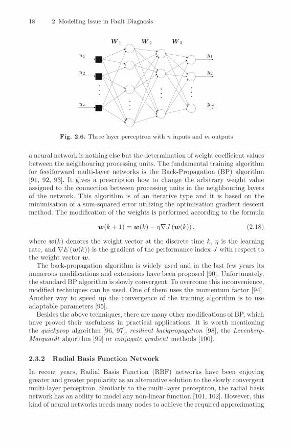
18 2 Modelling Issue in Fault Diagnosis
W 1 W 2 W 3
u1
u2
un
y1
y2
ym
�
�
� ��
�
� �
�
�
� �
Fig. 2.6. Three layer perceptron with n inputs and m outputs
a neural network is nothing else but the determination of weight coefficient valuesbetween the neighbouring processing units. The fundamental training algorithmfor feedforward multi-layer networks is the Back-Propagation (BP) algorithm[91, 92, 93]. It gives a prescription how to change the arbitrary weight valueassigned to the connection between processing units in the neighbouring layersof the network. This algorithm is of an iterative type and it is based on theminimisation of a sum-squared error utilizing the optimisation gradient descentmethod. The modification of the weights is performed according to the formula
w(k + 1) = w(k) − η∇J (w(k)) , (2.18)
where w(k) denotes the weight vector at the discrete time k, η is the learningrate, and ∇E (w(k)) is the gradient of the performance index J with respect tothe weight vector w.
The back-propagation algorithm is widely used and in the last few years itsnumerous modifications and extensions have been proposed [90]. Unfortunately,the standard BP algorithm is slowly convergent. To overcome this inconvenience,modified techniques can be used. One of them uses the momentum factor [94].Another way to speed up the convergence of the training algorithm is to useadaptable parameters [95].
Besides the above techniques, there are many other modifications of BP, whichhave proved their usefulness in practical applications. It is worth mentioningthe quickprop algorithm [96, 97], resilient backpropagation [98], the Levenberg-Marquardt algorithm [99] or conjugate gradient methods [100].
2.3.2 Radial Basis Function Network
In recent years, Radial Basis Function (RBF) networks have been enjoyinggreater and greater popularity as an alternative solution to the slowly convergentmulti-layer perceptron. Similarly to the multi-layer perceptron, the radial basisnetwork has an ability to model any non-linear function [101, 102]. However, thiskind of neural networks needs many nodes to achieve the required approximating
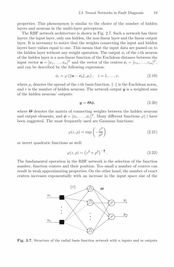
2.3 Neural Networks in Fault Diagnosis 19
properties. This phenomenon is similar to the choice of the number of hiddenlayers and neurons in the multi-layer perceptron.
The RBF network architecture is shown in Fig. 2.7. Such a network has threelayers: the input layer, only one hidden, the non-linear layer and the linear outputlayer. It is necessary to notice that the weights connecting the input and hiddenlayers have values equal to one. This means that the input data are passed on tothe hidden layer without any weight operation. The output φi of the i-th neuronof the hidden layer is a non-linear function of the Euclidean distance between theinput vector u = [u1, . . . , un]T and the vector of the centres ci = [ci1, . . . , cin]T ,and can be described by the following expression:
φi = ϕ (‖u − ci‖, ρi) , i = 1, . . . , v, (2.19)
where ρi denotes the spread of the i-th basis function, ‖·‖ is the Euclidean norm,and v is the number of hidden neurons. The network output y is a weighted sumof the hidden neurons’ outputs:
y = Θφ, (2.20)
where Θ denotes the matrix of connecting weights between the hidden neuronsand output elements, and φ = [φ1, . . . , φv]T . Many different functions ϕ(·) havebeen suggested. The most frequently used are Gaussian functions:
ϕ(z, ρ) = exp(
−z2
ρ2
)(2.21)
or invert quadratic functions as well:
ϕ(z, ρ) =(z2 + ρ2)− 1
2 . (2.22)
The fundamental operation in the RBF network is the selection of the functionnumber, function centres and their position. Too small a number of centres canresult in weak approximating properties. On the other hand, the number of exactcentres increases exponentially with an increase in the input space size of the
{1}Θ
u1
un
y1
ym�
��
�
�
�
Fig. 2.7. Structure of the radial basis function network with n inputs and m outputs

20 2 Modelling Issue in Fault Diagnosis
network. Hence, it is unsuitable to use the RBF network in problems wherethe input space has large sizes. To train such a network, hybrid techniques areused. First, the centres and the spreads of the basis functions are establishedheuristically. After that, the adjusting of the weights is performed. The centresof the radial basis functions can be chosen in many ways, e.g. as values of therandom distribution over the input space or by clustering algorithms [103, 104],which give statistically the best choice of the centre numbers and their positionsas well. When the centre values are established, the objective of the learningalgorithm is to determine the optimal weight matrix Θ, which minimises thedifference between the desired and the real network response. The output of thenetwork is linear in weights and that is why for the estimation of the weightmatrix traditional regressive methods can be used. Examples of such techniquesare the orthogonal least square method [105] and the Kaczmarz algorithm [104].The former guarantees fast convergence and fast training of the RBF network.On the contrary, Kaczmarz’s algorithm is less numerically complicated, but itis sometimes slowly convergent, for example, when system equations are badlyconditioned.
2.3.3 Kohonen Network
Kohonen network is a self-organizing map. Such a network can learn to detectregularities and correlations in their input and adapt their future responses tothat input accordingly. The network parameters are adpated by a learning pro-cedure based on input patterns only (unsupervised learning). Contrary to thestandard supervised learning methods, the unsupervised ones use input signalsto extract knowledge from data. During learning, there is no feedback to theenvironment or the investigated process. Therefore, neurons and weighted con-nections should have a certain level of self-organization. Moreover, unsupervisedlearning is only useful and effective when there is a redundancy of learningpatterns. Inputs and neurons in the competitive layer are connected entirely.Furthermore, the concurrent layer is the network output which generates theresponse of the Kohonen network. The weight parameters are adapted using thewinner takes all rule as follows [106]:
i = arg minj
{‖u − wj‖
}, (2.23)
where u is the input vector, i is the index of the winner, wj is the weight vectorof the j-th neuron. However, instead of adapting only the winning neuron, allneurons within a certain neighbourhood of the winning neuron are adjustedaccording to the formula
wj(k + 1) = wj(k) + η(k)C(k) (u(k) − wj(k)) , (2.24)
where η(k) is the learning rate and C(k) is a neighbourhood. The learning rateand the neighbourhood size are altered through two phases: an ordering phaseand a tunning phase. An iterative character of the learning rate leads to grad-ual establishing of the feature map. During the first phase, neuron weights are
2.3 Neural Networks in Fault Diagnosis 21
expected to order themselves in the input space consistent with the associatedneuron positions. During the second phase, the learning rate continues to de-crease, but very slowly. The small value of the learning rate finely tunes thenetwork while keeping the ordering learned in the previous phase stable. In theKohonen learning rule, the learning rate is a monotone decreasing time function.Frequently used functions are η(k) = 1/k or η(k) = ak−a for 0 < a � 1.
The concept of neighbourhood is extremely important during network pro-cessing. A suitably defined neighbourhood influences the number of adaptingneurons, e.g. 7 neurons belong to the neighbourhood of radius 1 defined on thehexagonal grid while the neighbourhood of radius 1 arranged on the rectangulargrid includes 9 neurons. A dynamic change of the neighbourhood size beneficiallyinfluences the quickness of feature map ordering. The learning process starts witha large neighbourhood size. Then, as the neighbourhood size decreases to 1, themap tends to order itself topologically over the presented input vectors. Oncethe neighbourhood size is 1, the network should be fairly well ordered and thelearning rate slowly decreases over a longer period to give the neurons time tospread out evenly across the input vectors. A typical neighbourhod function isthe Gaussian one [23, 90]. After designing the network, a very important taskis assigning clustering results generated by the network with desired results fora given problem. It is necessary to determine which regions of the feature mapwill be active during the occurrence of a given fault.
The remaining part of this section is devoted to different fault diagnosisschemes. Modern methods of FDI of dynamic systems can be split into threebroad cathegories: model based approaches, knowledge based approaches, anddata analysis based approaches. In the following sections, all three classes arediscussed with emphasis on the role of neural networks in each scheme.
2.3.4 Model Based Approaches
Model based approaches generally utilise results from the field of control the-ory and are based on parameter estimation or state estimation. The approach isfounded on the fact that a fault will cause changes in certain physical parameterswhich in turn will lead to changes in some model parameters or states. Whenusing this approach, it is essential to have quite accurate models of the processconsidered. Technological plants are often complex dynamic systems describedby non-linear high-order differential equations. For their quantitative modellingfor residual generation, simplifications are inevitable. This usually concerns boththe reduction of dynamics order and linearisation. Another problem arises fromunknown or time variant process parameters. Due to all these difficulties, con-ventional analytical models often turn out to be not accurate enough for effectiveresidual generation. In this case, knowledge based models are the only alterna-tive. For the model based approach, the neural network replaces the analyticalmodel that describes the process under normal operating conditions. First, thenetwork has to be trained for this task. The learning data can be collecteddirectly from the process, if possible, or from a simulation model that is as real-istic as possible. The latter possibility is of special interest for data acquisition

22 2 Modelling Issue in Fault Diagnosis
Faults f Disturbances d
PROCESS
Residual generation( Neural model)
Residual evaluation(Neural classifier)
Input u(k) Output y(k)
Residuals r
Faults f
Fig. 2.8. Model based fault diagnosis using neural networks
in different faulty situations in order to test the residual generator, as thosedata are not generally available in the real process. The training process canbe carried out off-line or on-line (it depends on the availability of data). Thepossibility to train a network on-line is very attractive, especially in the caseof adapting a neural model to mutable environment or non-stationary systems.After finishing the training, the neural network is ready for on-line residual gen-eration. To be able to capture the dynamic behaviour of the system, a neuralnetwork should have dynamic properties, e.g. it should be a recurrent network.Residual evaluation is a decision-making process that transforms quantitativeknowledge into qualitative Yes or No statements. It can also be seen as a clas-sification problem. The task is to match each pattern of the symptom vectorwith one of the pre-assigned classes of faults and the fault-free case. This pro-cess may highly benefit from the use of intelligent decision making. To performresidual evaluation, neural networks can be applied, e.g. feedforward networks orself-organizing maps. Figure 2.8 presents the block scheme of model based faultdiagnosis designed using neural networks. Neural networks have been success-fully applied to many applications including model based fault diagnosis. Amongmany, it is worth noting several applications. Neural networks have been usedin fault detection and classification in chemical processes: batch polymerisationand the distillation column [107]. Multi-layer feedforward networks with delayshave been used to model chemical processes, and the RBF network has beenapplied as a classifier. Chen and Lee used a neural network based scheme forfault detection and diagnosis in the framework of fault tolerant control in anF-16 aircraft simulator [108]. The authors of this work used an RBF networkwith delays to model full non-linear dynamics of an F-16 aircraft flight simulator.After that, with the help of the well-known multi-layer perceptron, a decisionabout faults was made. There is also a variety of papers showing the applicationof recurrent networks to model based fault diagnosis. A fault diagnosis schemeto detect and diagnose transient faults in a turbine waste gate of a diesel enginewas reported in [109]. An observer based fault detection and isolation system of a
2.3 Neural Networks in Fault Diagnosis 23
three-tank laboratory system was discussed in [39]. Model based fault diagnosisof sensor and actuator faults in a sugar evaporator using recurrent networks waspresented in [26].
2.3.5 Knowledge Based Approaches
Knowledge based approaches are generally based on expert or qualitative rea-soning [110]. Several knowledge based fault diagnosis approaches have been pro-posed. These include the rule based approach, where a diagnostic rule can beformulated from the process structure and unit functions, and the qualitativesimulation based approach. In the rule based approach, faults are usually diag-nosed by casually tracing symptoms backward along their propagation paths.Fuzzy reasoning can be used in the rule based approach to handle uncertain in-formation. In the qualitative simulation based approach, qualitative models of aprocess are used to predict the behaviour of the process under normal operatingconditions and in various faulty situations. Fault detection and diagnosis is thenperformed by comparing the predicted behaviour with the actual observations.The methods that fall into this category can be viewed as fault analysers be-cause their objective is to make a decision whether or not a fault has occuredin the system based on the set of logical rules that are either pre-programmedby an expert or learned through a training process (Fig. 2.9). When data aboutprocess states or operation condition are passed on to the fault analyser, theyare checked against the rule base stored there and a decision about operationconditions of the system is made. Neural networks are an excellent tool to de-sign such fault analysers [64]. The well-known feedforward multi-layer networksare most frequently used. Summarizing, to develop knowledge based diagnos-tic systems, knowledge about the process structure, process unit fuctions andqualitative models of process units under various faulty conditions are required.Therefore, the development of a knowledge based diagnosis system is generallyeffort demanding.
2.3.6 Data Analysis Approaches
In data analysis based approaches, process operational data covering variousnormal and abnormal operations are used to extract diagnostic knowledge. Twomain methods exist: neural network based fault diagnosis and multivariate statis-tical data analysis based fault diagnosis. In neural network based fault diagnosis,the only knowledge required is the training data, which contain faults and theirsymptoms. The fault symptoms are in the form of variations in process mea-surements. Through the training, the relationships between the faults and theirsymptoms can be discovered and stored as network weights. The trained net-work can be then used to diagnose faults in such a way that it can associate theobserved abnormal conditions with their corresponding faults. This group of ap-proached uses neural networks as pattern classifiers (Fig. 2.10). In multivariatestatistical data analysis techniques, fault signatures are extracted from process

24 2 Modelling Issue in Fault Diagnosis
Faults f Disturbances d
PROCESS
Generation ofdiagnostic signals(Neural network)
Input u(k) Output y(k)
Diagnostic signals s
Fig. 2.9. Model-free fault diagnosis using neural networks
operational data through some multivariate statistical methods such as princi-pal component analysis, projection to a latent structure or non-linear principalcomponent analysis [111]. It should be mentioned that statistical data analysissuch as principal component analysis can be carried out by means of neuralnetwork training, e.g. the Generalized Hebbian Algorithm (GHA) or AdaptivePrincipal-component EXtractor (APEX) algorithms, which utilize a single per-ceptron network or its modifications [23].
There is a rich bibliography reporting applications of neural networks in theframework of data analysis to fault diagnosis of technical and industrial pro-cesses. Karpenko and colleagues implemented a neural network of the feedfor-ward type to detect and identify actuator faults in a pneumatic control valve[112]. The network was trained to assign each operating condition to a specificclass, and to estimate the magnitude of the faulty condition. On-line fault di-agnosis of a continuous stirred tank reactor using a multiple neural network isreported in [113]. The achieved results confirmed that a multiple network struc-ture based system gives more reliable diagnosis than a single neural network. Inturn, a self-organizing competitive neural network was applied to fault diagnosisof the suck rod pumping system in [114]. The authors obtained a high qualityfault classifier performing better than a classical feedforward network.
Neural networks can be also useful in the area of feature extraction. G�lowackiand co-workers used the multi-layer feedforward network trained with theLevenberg-Marquardt algorithm for fault detection of a DC motor [115]. A sim-ilar approach was used in [116] for sensor fault isolation and reconstruction.
2.4 Evaluation of the FDI System
Each diagnostic algorithm or method should be validated to confirm its effec-tiveness and usefulness for real-world fault diagnosis. In this section, we define aset of indices needed to evaluate an FDI system. The benchmark zone is definedfrom the benchmark start-up time ton to the benchmark time horizon thor.

2.4 Evaluation of the FDI System 25
Faults f Disturbances d
PROCESS
Extraction ofdiagnostic
signals
Classification(Neural network)
Faultpatterns
Input u(k) Output y(k)
Diagnostic signals s
Faults f
Fig. 2.10. Fault diagnosis as pattern recognition
ton tfrom thor time
timetdt
Res
idual
Dec
isio
nm
akin
g
0
1
true decisionsfalsedecisions
���� � ���
Fig. 2.11. Definition of the benchmark zone
Figure 2.11 illustates the benchmark zone definition. Decisions before the bench-mark start-up ton and after the benchmark time horizon thor are out of interest.The time of the fault start-up is represented by tfrom. When a fault occurs inthe system, a residual should deviate from the level assigned to the fault-freecase (Fig. 2.11). The quality of the fault detection system can be evaluated usinga number of performance indices [52, 26]:
26 2 Modelling Issue in Fault Diagnosis
• Time of fault detection tdt – period of time needed for the detection of afault measured from tfrom to a permanent, true decision about a fault, aspresented in Fig. 2.11. As one can see there, the first three true decisions aretemporary ones and are not taken into account during determining tdt;
• False detection rate rfd defined as follows:
rfd =
∑i tifd
tfrom − ton, (2.25)
where tifd is the period of the i-th false fault detection. This index is used tocheck the system in the fault-free case. Its value shows the percentage of falsealarms. In the ideal case (no false alarms), its value should be equal to 0;
• True detection rate rtd given by
rtd =∑
i titdthor − tfrom
, (2.26)
where titd is the period of the i-th true fault detection. This index is used inthe case of faults and describes the efficiency of fault detection. In the idealcase (fault detected immediately and surely), its value is equal to 1;
• Isolation time tit – period of time from the beginning of the fault start-uptfrom to the moment of fault isolation;
• False isolation rate rfi represented by the formula
rfi =
∑i tifi
tfrom − ton, (2.27)
where tifi is the period of the i-th false fault isolation;• True isolation rate rti defined by the following equation:
rti =∑
i titithor − tfrom
, (2.28)
where titi is the period of the i-th true fault isolation.
2.5 Summary
The diagnostics of industrial processes is a scientific discipline which has beenexpansively developed in recent years. It is very difficult to imagine a big indus-trial plant without a monitoring or diagnostic system. It is clear that providingfast and reliable fault diagnosis is a part of control design. Unfortunately, mostcontrol systems exhibit non-linear behaviour, which makes it impossible to useclasical methods such as parameter estimation methods, parity relations or ob-servers. Taking into account the above, there is a need for techniques able tocope with non-linearities. One possible solution is to use artificial intelligencemethods. Artificial neural networks have gained a more and more prominent

2.5 Summary 27
position in fault detection systems. The chapter presented three main classes offault diagnosis methods, i.e. model based, knowledge based and data analysisbased approaches with emphasis on neural networks’ role in these schemes. Gen-erally, based on the presented case studies, neural networks can be used in twoways: to construct a model of the process considered or to perform classificationtasks.
In the further part of this book neural networks are discussed in the frameworkof modelling and model based fault diagnosis. Special attention is paid to theso-called locally recurrent networks. In order to properly use the dynamic typeof neural networks for modelling or residual generation, a number of problemshas to be solved, e.g. deriving training algorithms, investigating approximationabilities and stability problems, and selecting optimal training sequences. Theseproblems are presented in the forthcoming chapters. Neural network based al-gorithms for residual evaluation are also considered.

3 Locally Recurrent Neural Networks
Artificial neural networks provide an excellent mathematical tool for dealing withnon-linear problems [18, 23, 77]. They have an important property according towhich any continuous non-linear relation can be approximated with arbitraryaccuracy using a neural network with a suitable architecture and weight pa-rameters. Their another attractive property is the self-learning ability. A neuralnetwork can extract the system features from historical training data using thelearning algorithm, requiring little or no a priori knowledge about the process.This provides the modelling of non-linear systems with a great flexibility [18, 19].However, the application of neural networks to the modelling or fault diagno-sis of control systems requires taking into account the dynamics of processes orsystems considered. A neural network to be dynamic must contain a memory.The memory can be divided into a short-term memory and a long-term mem-ory, depending on the retention time [117, 36, 118, 23]. The short-term memoryrefers to a compilation of knowledge representing the current state of the envi-ronment. In turn, the long-term memory refers to knowledge stored for a longtime or permanently. One simple way of incorporating a memory into the struc-ture of a neural network is the use of time delays, which can be implemented atthe synaptic level or in the input layer of the network. Another important wayin which the dynamics can be built into the operation of a neural network ina implicit manner is through the use of feedbacks. The are two basic methodsof incorporating feedbacks to a neural network: local feedback at the level of asingle neuron inside the network and global feedback encompassing the wholenetwork. Neural networks with one or more feedbacks are referred to as recurrentnetworks. This chapter is mainly focused on locally recurrent networks.
The chapter is organized as follows: the first part, consiting of Sections 3.1,3.2, 3.3 and 3.4, deals with network structures, in which dynamics are realizedusing time delays and global feedbacks. Section 3.5 presents locally recurrentstructures, with the main emphasis on networks designed with neuron modelswith infinite impulse response filters. Training methods intended for use withlocally recurrent networks are described in Section 3.6. Three algorithms areproposed: extentded dynamic back-propagation, adaptive random search and
K. Patan: Artificial. Neural Net. for the Model. & Fault Diagnosis, LNCIS 377, pp. 29–63, 2008.springerlink.com c© Springer-Verlag Berlin Heidelberg 2008
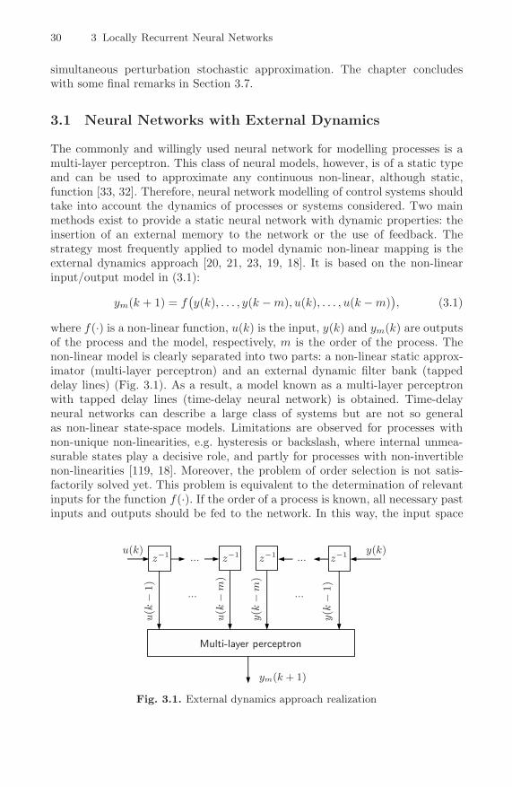
30 3 Locally Recurrent Neural Networks
simultaneous perturbation stochastic approximation. The chapter concludeswith some final remarks in Section 3.7.
3.1 Neural Networks with External Dynamics
The commonly and willingly used neural network for modelling processes is amulti-layer perceptron. This class of neural models, however, is of a static typeand can be used to approximate any continuous non-linear, although static,function [33, 32]. Therefore, neural network modelling of control systems shouldtake into account the dynamics of processes or systems considered. Two mainmethods exist to provide a static neural network with dynamic properties: theinsertion of an external memory to the network or the use of feedback. Thestrategy most frequently applied to model dynamic non-linear mapping is theexternal dynamics approach [20, 21, 23, 19, 18]. It is based on the non-linearinput/output model in (3.1):
ym(k + 1) = f(y(k), . . . , y(k − m), u(k), . . . , u(k − m)
), (3.1)
where f(·) is a non-linear function, u(k) is the input, y(k) and ym(k) are outputsof the process and the model, respectively, m is the order of the process. Thenon-linear model is clearly separated into two parts: a non-linear static approx-imator (multi-layer perceptron) and an external dynamic filter bank (tappeddelay lines) (Fig. 3.1). As a result, a model known as a multi-layer perceptronwith tapped delay lines (time-delay neural network) is obtained. Time-delayneural networks can describe a large class of systems but are not so generalas non-linear state-space models. Limitations are observed for processes withnon-unique non-linearities, e.g. hysteresis or backslash, where internal unmea-surable states play a decisive role, and partly for processes with non-invertiblenon-linearities [119, 18]. Moreover, the problem of order selection is not satis-factorily solved yet. This problem is equivalent to the determination of relevantinputs for the function f(·). If the order of a process is known, all necessary pastinputs and outputs should be fed to the network. In this way, the input space
ym(k + 1)
u(k
−m
)
u(k
−1)
y(k
−m
)
y(k
−1)
Multi-layer perceptron
z−1z−1z−1z−1u(k) y(k)
... ...
... ...
Fig. 3.1. External dynamics approach realization
3.2 Fully Recurrent Networks 31
of the network becomes large. In many practical cases, there is no possibility tolearn the order of the modelled process, and the number of suitable delays hasto be selected experimentally by using the trial and error procedure [19].
Many papers show that the multi-layer perceptron is able to predict the out-puts of various dynamic processes with high precision, but its inherent non-linearity makes assuring stability a hard task, especially in the cases in whichthe output of the network is fed back to the network input as in the case of theparallel model [20, 19]. There are also situations in which this type of networksis not capable of capturing the whole plant state information of the modelledprocess [120, 119].
The use of real plant outputs avoids many of the analytical difficulties encoun-tered, assures stability and simplifies the identification procedure. This type offeedforward networks is known as a series-parallel model, introduced by Naren-dra and Parthasarathy [20]. Such networks are capable of modelling systems ifthey have a weakly visible state, i.e. if there is an input-output equivalent to asystem whose state is a function or a fixed set of finitely many past values of itsinputs and outputs [120]. Otherwise, the model has a strongly hidden state andits identification requires recurrent networks of a fairly general type.
Recurrent networks are neural networks with one or more feedback loops.As a result of feedbacks introduced to the network structure, it is possible toaccumulate the information and use it later. Feedbacks can be either of a local ora global type. Taking into account the possible location of feedbacks, recurrentnetworks can be divided as follows [38, 23, 40]:
• Globally recurrent networks – there are feedbacks allowed between neurons ofdifferent layers or between neurons of the same layer. Such networks incorpo-rate a static multi-layer perceptron or parts of it. Moreover, they exploit thenon-linear mapping capability of the multi-layer perceptron. Basically, threekinds of networks can be distinguished [29, 18]:� fully recurrent networks,� partially recurrent networks,� state-space networks;
• Locally recurrent networks – there are feedbacks only inside neuron models.This means that there are neither feedback connections between neurons ofsuccessive layers nor lateral links between neurons of the same layer. Thesenetworks have a structure similar to static feedforward ones, but consist ofthe so-called dynamic neuron models.
3.2 Fully Recurrent Networks
The most general architecture of the recurrent neural network was proposedby Williams and Zipser in [35]. This structure is often called the Real TimeRecurrent Network (RTRN), because it has been designed for real time signalprocessing. The network consists of M neurons, and each of them creates feed-back. Each link between two neurons represents an internal state of the model.Any connections between neurons are allowed. Thus, a fully connected neural

32 3 Locally Recurrent Neural Networks
m
m+1
1
M
u1(k)
un(k)
y1(k + 1)
ym(k + 1)
z−1
z−1
z−1
z−1
...
...
...
Fig. 3.2. Fully recurrent network of Williams and Zipser
architecture is obtained. Only m of M neurons are established as the outputunits. The remaining H = M − m neurons are hidden ones. The scheme ofthe RTRN architecture with n inputs and m outputs is shown in Fig. 3.2. Thisnetwork is not organized in layers and has no feedforward architecture. The fun-damental advantage of such networks is the possibility of approximating wideclass of dynamic relations. Such a kind of networks, however, exhibits somewell-known disadvantages. First of them is a large structural complexity; O(n2)weights needed for n neurons. Also, the training of the network is usually complexand slowly convergent [29, 23, 40]. Moreover, there are problems with keepingnetwork stability. Generally, this dynamic structure seems to be too complex forpractical applications. Moreover, the fixed relation between the number of statesand the number of neurons does not allow one to adjust the dynamics order andnon-linear properties of the model separately. Bearing in mind these disadvan-tages, fully recurrent networks are rather not used in engineering practice ofnon-linear system identification.
3.3 Partially Recurrent Networks
Partially recurrent networks have a less general character [121, 122, 36, 123].Contrary to the fully recurrent network, the architecture of partially recurrentnetworks is based on a feedforward multi-layer perceptron consisting of an ad-ditional layer of units called the context layer. Neurons of this layer serve asinternal states of the model. Among many proposed structures, two partiallyrecurrent networks have received considerable attention: the Elman [36] and theJordan [123] structure. The Elman network is probably the best-known exam-ple of a partially recurrent neural network. The realization of such networks isconsiderably less expensive than in the case of a multi-layer perceptron withtapped delay lines. The scheme of the Elman network is shown in Fig. 3.3(a).This network consists of four layers of units: the input layer with n units, thecontext layer with v units, the hidden layer with v units and the output layer

3.3 Partially Recurrent Networks 33
un(k)
u1(k)
...
...
conte
xtla
yer
copy madeeach time
step
...
...
ym(k)
y1(k)
(a)
un(k)
u1(k)
...
...
conte
xtla
yer
copy made eachtime step
...
...
ym(k)
y1(k)
(b)
Fig. 3.3. Partialy recurrent networks due to Elman (a) and Jordan (b)
with m units. The input and output units interact with the outside environment,whereas the hidden and context units do not. The context units are used onlyto memorize the previous activations of the hidden neurons. A very importantassumption is that in the Elman structure the number of context units is equalto the number of hidden units. All the feedforward connections are adjustable;the recurrent connections denoted by a thick arrow in Fig. 3.3(a) are fixed. The-oretically, this kind of networks is able to model the s-th order dynamic system,if it can be trained to do so [23]. At the specific time k, the previous activationof the hidden units (at time k − 1) and the current inputs (at time k) is used asinputs to the network. In this case, the Elman network’s behaviour is analogousto that of a feedforward network. Therefore, the standard back-propagation al-gorithm can be applied to train the network parameters. However, it should bekept in mind that such simplifications limit the application of the Elman struc-ture to the modelling of dynamic processes [29, 28]. In turn, the Jordan networkis presented in Fig. 3.3(b). In this case, feedback connections from the outputneurons are fed to the context units. The Jordan network has been succesfullyapplied to recognize and differentiate various output time-sequences [124, 123]or to classify English syllables [125].
Partially recurrent networks possess over fully recurrent networks the ad-vantage that their recurrent links are more structured, which leads to fastertraining and fewer stability problems [23, 18]. Newerless, the number of statesis still strongly related to the number of hidden (for Elman) or output (for Jor-dan) neurons, which severely restricts their flexibility. In the literature, there arepropositions to extend partially recurrent networks by introducing additional re-current links, represented by the weight α, from the context units to themselves[121, 126]. The value of α should be less than 1. For α close to 1, the long termmemory can be obtained, but it is less sensitive to details.
Another architecture can be found in the recurrent network elaborated byParlos [37] (Fig. 3.4). A Recurrent Multi-Layer Perceptron (RMLP) is designed

34 3 Locally Recurrent Neural Networks
u1(k)
u2(k)
un(k)
y1(k)
y2(k)
ym(k)
recurrentlinks
cross-talklinks
feedforwardlinks
...
...
Fig. 3.4. Architecture of the recurrent multi-layer perceptron
based on the multi-layer perceptron network, and by adding delayed links be-tween neighbouring units of the same hidden layer (cross-talk links), includingunit feedback on itself (recurrent links) [37]. Empirical evidence indicates thatby using delayed recurrent and cross-talk weights the RMLP network is able toemulate a large class of non-linear dynamic systems. The feedforward part of thenetwork still maintains the well-known curve-fitting properties of the multi-layerperceptron, while the feedback part provides its dynamic character. Moreover,the usage of the past process observations is not necessary, because their effect iscaptured by internal network states. The RMLP network has been successfullyused as a model for dynamic system identification [37]. However, a drawback ofthis dynamic structure is increased network complexity strictly dependent on thenumber of hidden neurons and the resulting long training time. For the networkcontaining one input, one output and only one hidden layer with v neurons, thenumber of the network parameters is equal to v2 + 3v.
3.4 State-Space Networks
Figure 3.5 shows another type of recurrent neural networks known as the state-space neural network [119, 23, 18]. The output of the hidden layer is fed back to
bank ofunit
delays
non-linearhiddenlayer
linearoutputlayer
bank ofunit
delaysu(k)
x(k)
x(k+1)
y(k+1) y(k)
Fig. 3.5. Block scheme of the state-space neural network with one hidden layer

3.4 State-Space Networks 35
the input layer through a bank of unit delays. The number of unit delays usedhere determines the order of the system. The user can choose how many neuronsare used to produce feedback. Let u(k) ∈ R
n be the input vector, x(k) ∈ Rq –
the output of the hidden layer at time k, and y(k) ∈ Rm – the output vector.
Then the state-space representation of the neural model presented in Fig. 3.5 isdescribed by the equations
x(k + 1) = f (x(k), u(k)),
(3.2)
y(k) = Cx(k) (3.3)
where f(·) is a non-linear function characterizing the hidden layer, and C isa matrix of synaptic weights between hidden and output neurons. This modellooks similar to the external dynamic approach presented in Fig. 3.1, but themain difference is that for the external dynamics the outputs which are fed backare known during training, while for the state-space model the outputs whichare fed back are unknown during training. As a result, state-space models can betrainined only by minimizing the simulation error. State-space models possess anumber of advantages, contrary to fully and partially recurrent networks [23, 18]:
• The number of states (model order) can be selected independently from thenumber of hidden neurons. In this way only those neurons that feed theiroutputs back to the input layer through delays are responsible for definingthe state of the network. As a consequence, the output neurons are excludedfrom the definition of the state;
• Since model states feed the input of the network, they are easily accesiblefrom the outside environment. This property can be useful when state mea-surements are available at some time instants (e.g. initial conditions).
The state-space model includes several recurrent structures as special cases.The previously analyzed Elman network has an architecture similar to that pre-sented in Fig. 3.5, except for the fact that the output layer can be non-linearand the bank of unit delays at the output is omitted.
In spite of the fact that state-space neural networks seem to be more promisingthan fully or partially neural networks, in practice a lot of difficulties can beencountered [18]:
• Model states do not approach true process states;• Wrong initial conditions can deteriorate the performance, especially when
short data sets are used for training;• Training can become unstable;• The model after training can be unstable.
In particular, these drawbacks appear in the cases when no state measurementsand no initial conditions are available.
A very important property of the state-space neural network is that it can ap-proximate a wide class of non-linear dynamic systems [119]. There are, however,some restrictions. The approximation is only valid on compact subsets of thestate-space and for finite time intervals, thus interesting dynamic characteristicsare not reflected [127, 23].

36 3 Locally Recurrent Neural Networks
3.5 Locally Recurrent Networks
All recurrent networks described in the previous sections are called globallyrecurrent neural networks. In such networks all possible connections betweenneurons are allowed, but all of the neurons in a network structure are static onesbased on the McCulloch-Pitts model.
A biological neural cell not only contains a non-linear mapping operation onthe weighted sum of its inputs but it also has some dynamic properties suchas state feedbacks, time delays hysteresis or limit cycles. In order to cope withsuch dynamic behaviour, a special kind of neuron models has been proposed[128, 129, 130, 131, 132]. Such neuron models constitute a basic building blockfor designing a complex dynamic neural network.
The dynamic neuron unit systematized by Gupta and co-workers in [77] as thebasic element of neural networks of the dynamic type is presented in Fig. 3.6(a).The neuron receives not only external inputs but also state feedback signals fromitself and other neurons in the network. The synaptic links in this model containa self-recurrent connection representing a weighted feedback signal of its stateand lateral connections which constitute state feedback from other neurons ofthe network. The dynamic neuron unit is connected to other (n − 1) modelsof the same type forming a neural network (Fig. 3.6(b)). The general dynamicneuron unit is described by the following equations:
dxi(t)dt
= −αixi(t) + fi(wi, x),
(3.4)
yi(t) = gi(xi(t)) (3.5)
where x ∈ Rn+1 is the augmented vector of n-neural states from other neurons
in the network including the bias, wi is the vector of synaptic weights associatedwith the i-th dynamic neuron unit, αi is the feedback parameter of the i-thdynamic unit, yi(t) is the output of the i-th neuron, fi(·) is a non-linear function
-αi
self-recurrence
fi gi1s
+yi(k)x(k)
xi(k)
self-feedback
(a) lateralrecurrence
self-recurrence
dynamic neuron unit
inputs
outp
uts
(b)
Fig. 3.6. Generalized structure of the dynamic neuron unit (a), network composed ofdynamic neural units (b)
3.5 Locally Recurrent Networks 37
of the i-th neuron, and gi(·) is an output function of the i-th neuron. UsingEuler’s method, the first order derivative is approximated as
dx(t)dt
∣∣∣t=kT
=x((k + 1)T ) − x(kT )
T, (3.6)
where T stands for the sampling time and k is the discrete-time index. Assumingthat T = 1, (3.6) can be rewritten in the simpler form
dx(t)dt
= x(k + 1) − x(k). (3.7)
Using (3.7), the discrete-time forms of (3.4) and (3.5) are as follows:
xi(k + 1) = −(αi − 1)xi(k) + fi(wi, x(k)).
(3.8)
yi(k) = gi(xi(k)) (3.9)
Due to various choices of the functions fi(·) and gi(·) in (3.8) and (3.9) as wellas different types of synaptic connections, different dynamic neuron modelscan be obtained. The general discrete-time model described by (3.8) and (3.9)may be expanded into various other representations. Mathematical details ofdifferent types of dynamic neuron units are given in Table 3.1. Neural networkscomposed of dynamic neuron units have a recurrent structure with lateral linksbetween neurons, as depicted in Fig. 3.6(b). A different approach providingdynamically driven neural networks is used in the so-called Locally RecurrentGlobally Feed-forward (LRGF) networks [38, 40]. LRGF networks have anarchitecture that is somewhere inbetween a feedforward and a globally recurrentarchitecture. The topology of such a kind of neural networks is analogous tothe multi-layered feedforward one, and the dynamics are reproduced by theso-called dynamic neuron models. Based on the well-known McCulloch-Pittsneuron model, different dynamic neuron models can be designed. In general,differences between these depend on the localization of internal feedbacks.
Model with local activation feedback. This neuron model was studiedby Frasconi [130], and may be described by the following equations:
ϕ(k) =n∑
i=1
wiui(k) +r∑
i=1
diϕ(k − i),
(3.10a)
y(k) = σ(ϕ(k)
)(3.10b)
where ui, i = 1, 2, . . . , n are the inputs to the neuron, wi reflects the inputweights, ϕ(k) is the activation potential, di, i = 1, 2, . . . , r are the coefficientswhich determine feedback intensity of ϕ(k − i), and σ(·) is a non-linear acti-vation function. With reference to Fig. 3.7, the input to the neuron can bea combination of input variables and delayed versions of the activation ϕ(k).Note that right-hand side summation in (3.10a) can be interpreted as the Finite

38 3 Locally Recurrent Neural Networks
Table 3.1. Specification of different types of dynamic neuron units
Model fi(·) gi(·) Reference
DNU-1 wTi σ(x(k)) some function based on Hopfield
[133]
where σ(·) is a vector-valued activation function
DNU-2 wTi y(k) σi(xi(k)) based on Hopfield
[133]
where σi(·) is a non-linear activation functionof the i-th neuron
DNU-3 σi(wTi x(k)) xi(k) Pineda [134]
DNU-4 σi(wTi x(k)) + x0w0i xi(k) Pineda [135]
where wi ∈ Rn is the vector of synaptic weights
of the i-th neuron without bias, w0i is the biasof the i-th neuron
DNU-5 (γi − βixi)(wT
i σ(x(k)))
σi(xi(k)) Grossberg [136]
where γi is an automatic gain control of the i-thneuron, βi is a total normalization for theinternal state of the i-th neuron
Impulse Response (FIR) filter. This neuron model has the feedback signal takenbefore the non-linear activation block (Fig. 3.7).
Model with local synapse feedback. Back and Tsoi [129] introduced theneuron architecture with local synapse feedback (Fig. 3.8). In this structure,instead of a synapse in the form of the weight, the synapse with a linear trans-fer function, the Infinite Impulse Response (IIR) filter, with poles and zeros isapplied. In this case, the neuron is described by the following set of equations:
y(k) = σ
(n∑
i=1
Gi(z−1)ui(k)
),
(3.11a)
Gi(z−1) =
∑rj=0 bjz
−j∑pj=0 ajz−j
(3.11b)
where ui(k), i = 1, 2, . . . , n is the set of inputs to the neuron, Gi(z−1) is the lineartransfer function, bj , j = 0, 1, . . . , r, and aj , j = 0, 1, . . . , p are its zeros and poles,

3.5 Locally Recurrent Networks 39
w1
w2
wn
+ σ(·)
d1 d2 dr. . .
...
...
z−1 z−1 z−1
u1(k)
u2(k)
un(k)
ϕ(k) y(k)
Fig. 3.7. Neuron architecture with local activation feedback
respectively. As seen in (3.11b), the linear transfer function has r zeros and ppoles. Note that the inputs ui(k), i = 1, 2, . . . , n may be taken from the outputsof the previous layer, or from the output of the neuron. If they are derived fromthe previous layer, then it is local synapse feedback. On the other hand, if theyare derived from the output y(k), it is local output feedback. Moreover, localactivation feedback is a special case of the local synapse feedback architecture.In this case, all synaptic transfer functions have the same denominator and onlyone zero, i.e. bj = 0, j = 1, 2, . . . , r.
Model with local output feedback. Another dynamic neuron architecturewas proposed by Gori [128] (see Fig. 3.9). In contrast to local synapse as well aslocal activation feedback, this neuron model takes feedback after the non-linearactivation block. In a general case, such a model can be described as follows:
y(k) = σ
(n∑
i=1
wiui(k) +r∑
i=1
diy(k − i)
), (3.12)
where di, i = 1, 2, . . . , r are the coefficients which determine feedback intensityof the neuron output y(k − i). In this architecture, the output of the neuron isfiltered by the FIR filter, whose output is added to the inputs, providing theactivation. It is easy to see that by the application of the IIR filter to filteringthe neuron output a more general structure can be obtained [38]. The work ofGori [128] found its basis in the work by Mozer [122]. In fact, one can considerthis architecture as a generalization of the Jordan-Elman architecture [123, 36].
G1(z)
G2(z)
Gn(z)
+ σ(·)
...
u1(k)
u2(k)
un(k)
y(k)
Fig. 3.8. Neuron architecture with local synapse feedback

40 3 Locally Recurrent Neural Networks
w1
w2
wn
+ σ(·)
d1 d2 dr. . .
...
...
z−1 z−1 z−1
u1(k)
u2(k)
un(k)
ϕ(k) y(k)
Fig. 3.9. Neuron architecture with local output feedback
Memory neuron. Memory neuron networks were introduced by Poddarand Unnikrishnan [131]. These networks consist of neurons which have amemory; i.e. they contain information regarding past activations of its parentnetwork neurons. A general scheme of the memory neuron is shown in Fig. 3.10.The mathematical description of such a neuron is presented below:
y(k) = σ
(n∑
i=1
wiui(k) +n∑
i=1
sizi(k)
)(3.13a)
zi(k) = αiui(k − 1) + (1 − αi)zi(k − 1),
(3.13b)
where zi, i = 1, 2, . . . , n are the outputs of the memory neuron from the previouslayer, si, i = 1, 2, . . . , n are the weight parameters of the memory neuron outputzi(k), and αi = const is a coefficient. It is observed that the memory neuron”remembers” the past output values to that particular neuron. In this case,the memory is taken to be in the form of an expotential filter. This neuronstructure can be considered to be a special case of the generalized local outputfeedback architecture. It has a feedback transfer function with one pole only.Memory neuron networks have been intensively studied in recent years, andthere are some interesting results concerning the use of this architecture in theidentification and control of dynamic systems [137].
3.5.1 Model with the IIR Filter
In the following part of the section, the general structure of the neuron modelproposed by Ayoubi [109] is considered. The dynamics are introduced to theneuron in such a way that neuron activation depends on its internal states.This is done by introducing an IIR filter into the neuron structure. In this way,the neuron reproduces its own past inputs and activations using two signals:the input ui(k), for i = 1, 2, . . . , n and the output y(k). Figure 3.11 shows thestructure of the neuron model considered. Three main operations are performedin this dynamic structure. First of all, the weighted sum of inputs is calculatedaccording to the formula

3.5 Locally Recurrent Networks 41
memoryneuron
w1
w2
wn
+ σ(·)
zi(k)
αi
1−αi
...
z−1
z−1
u1(k)
u2(k)
un(k)
si
y(k)
+
Fig. 3.10. Memory neuron architecture
ϕ(k) =n∑
i=1
wiui(k). (3.14)
The weights perform a similar role as in static feedforward networks. The weightstogether with the activation function are responsible for approximation proper-ties of the model. Then this calculated sum ϕ(k) is passed to the IIR filter. Here,the filters under consideration are linear dynamic systems of different orders,viz. the first or the second order. The filter consists of feedback and feedforwardpaths weighted by the weights ai, i = 1, 2, . . . , r and bi, i = 0, 1, . . . , r, respec-tively. The behaviour of this linear system can be described by the followingdifference equation:
z(k) =r∑
i=0
biϕ(k − i) −r∑
i=1
aiz(k − i), (3.15)
where ϕ(k) is the filter input, z(k) is the filter output, and k is the discrete-timeindex. Alternatively, the equation (3.15) may by rewritten as a transfer function:
G(z) =∑n
i=0 bizi
1 +∑n
i=1 aizi. (3.16)
Finally, the neuron output can be described by
y(k) = σ(g2(z(k) − g1)
), (3.17)
w1
w2
wn
+ σ(·)IIR
...
u1(k)
u2(k)
un(k)
y(k)z(k)ϕ(k)
Fig. 3.11. Neuron architecture with the IIR filter
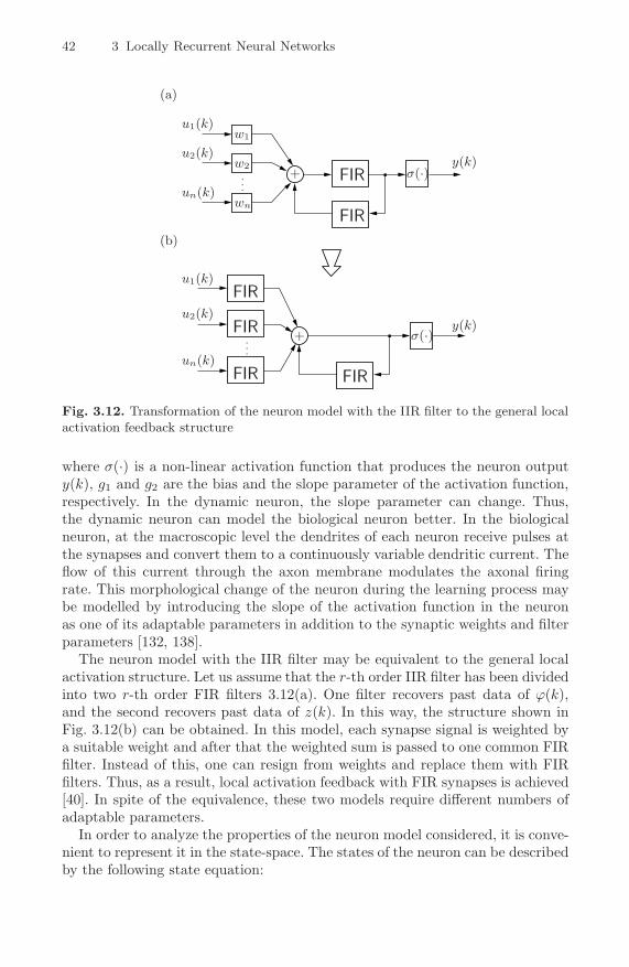
42 3 Locally Recurrent Neural Networks
(a)
(b)
FIR
FIR
FIR
+ σ(·)
FIR
...
u1(k)
u2(k)
un(k)
y(k)
u1(k)
u2(k)
un(k)
w1
w2
wn
FIR
FIRy(k)
+ σ(·)
...
Fig. 3.12. Transformation of the neuron model with the IIR filter to the general localactivation feedback structure
where σ(·) is a non-linear activation function that produces the neuron outputy(k), g1 and g2 are the bias and the slope parameter of the activation function,respectively. In the dynamic neuron, the slope parameter can change. Thus,the dynamic neuron can model the biological neuron better. In the biologicalneuron, at the macroscopic level the dendrites of each neuron receive pulses atthe synapses and convert them to a continuously variable dendritic current. Theflow of this current through the axon membrane modulates the axonal firingrate. This morphological change of the neuron during the learning process maybe modelled by introducing the slope of the activation function in the neuronas one of its adaptable parameters in addition to the synaptic weights and filterparameters [132, 138].
The neuron model with the IIR filter may be equivalent to the general localactivation structure. Let us assume that the r-th order IIR filter has been dividedinto two r-th order FIR filters 3.12(a). One filter recovers past data of ϕ(k),and the second recovers past data of z(k). In this way, the structure shown inFig. 3.12(b) can be obtained. In this model, each synapse signal is weighted bya suitable weight and after that the weighted sum is passed to one common FIRfilter. Instead of this, one can resign from weights and replace them with FIRfilters. Thus, as a result, local activation feedback with FIR synapses is achieved[40]. In spite of the equivalence, these two models require different numbers ofadaptable parameters.
In order to analyze the properties of the neuron model considered, it is conve-nient to represent it in the state-space. The states of the neuron can be describedby the following state equation:

3.5 Locally Recurrent Networks 43
Ai
b0
bz−1w 1 σ(·)y(k)u(k)
xi(k)xi(k+1)
++
Fig. 3.13. State-space form of the i-th neuron with the IIR filter
x(k + 1) = Ax(k) + Wu(k), (3.18)
where x(k) ∈ Rr is the state vector, W = 1wT is the weight matrix (w ∈ R
n,1 ∈ R
r is the vector with one in the first place and zeros elsewhere), u(k) ∈ Rn
is the input vector, n is the number of inputs, and the state matrix A has theform
A =
⎡⎢⎢⎢⎢⎢⎣
−a1 −a2 . . . −ar−1 −ar
1 0 . . . 0 00 1 . . . 0 0...
.... . .
......
0 0 . . . 1 0
⎤⎥⎥⎥⎥⎥⎦ . (3.19)
Finally, the neuron output is described by
y(k) = σ(g2(bx(k) + du(k) − g1)
), (3.20)
where σ(·) is a non-linear activation function, b = [b1 − b0a1, . . . , br − b0ar]is the vector of feedforward filter parameters, d = [b0w1, . . . , b0wn]. The blockstructure of the state-space representation of the neuron considered is presentedin Fig. 3.13.
3.5.2 Analysis of Equilibrium Points
Let x∗ be an equilibrium state of the dynamic neuron described by (3.18). In-troducing an equivalent transformation z(k) = x(k)−x∗, the system (3.18) canbe transformed to the form
z(k + 1) = Az(k). (3.21)
A constant vector z is said to be an equilibrium (stationary) state of the system(3.21) if the following condition is satisfied:
Az(k) = 0. (3.22)
If a matrix A is non-singular, the equilibrium state is determined by the eigen-values of A. If one assumes that the dynamic neuron consists of a second orderlinear dynamic system, equilibrium points may be divided into six classes de-picted in Fig. 3.14. The cases (a) and (b) show stable equilibrium points, while
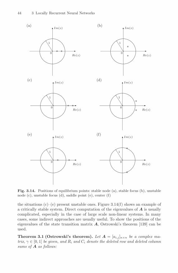
44 3 Locally Recurrent Neural Networks
Im(z)
Re(z)0
1
∗∗
(a)Im(z)
Re(z)0
1∗
∗
(b)
Im(z)
Re(z)0
1
∗ ∗
(c)Im(z)
Re(z)0
1∗
∗
(d)
Im(z)
Re(z)0
1
∗ ∗
(e)Im(z)
Re(z)0
1∗
∗
(f)
Fig. 3.14. Positions of equilibrium points: stable node (a), stable focus (b), unstablenode (c), unstable focus (d), saddle point (e), center (f)
the situations (c)–(e) present unstable ones. Figure 3.14(f) shows an example ofa critically stable system. Direct computation of the eigenvalues of A is usuallycomplicated, especially in the case of large scale non-linear systems. In manycases, some indirect approaches are usually useful. To show the positions of theeigenvalues of the state transition matrix A, Ostrowski’s theorem [139] can beused.
Theorem 3.1 (Ostrowski’s theorem). Let A = [ai,j ]n×n be a complex ma-trix, γ ∈ [0, 1] be given, and Ri and Ci denote the deleted row and deleted columnsums of A as follows:
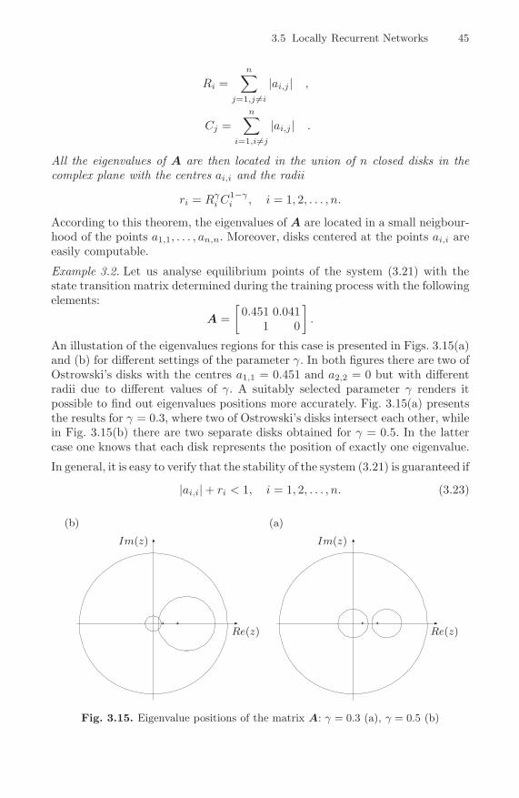
3.5 Locally Recurrent Networks 45
Ri =n∑
j=1,j �=i
|ai,j | ,
Cj =n∑
i=1,i�=j
|ai,j | .
All the eigenvalues of A are then located in the union of n closed disks in thecomplex plane with the centres ai,i and the radii
ri = Rγi C1−γ
i , i = 1, 2, . . . , n.
According to this theorem, the eigenvalues of A are located in a small neigbour-hood of the points a1,1, . . . , an,n. Moreover, disks centered at the points ai,i areeasily computable.
Example 3.2. Let us analyse equilibrium points of the system (3.21) with thestate transition matrix determined during the training process with the followingelements:
A =[
0.451 0.0411 0
].
An illustation of the eigenvalues regions for this case is presented in Figs. 3.15(a)and (b) for different settings of the parameter γ. In both figures there are two ofOstrowski’s disks with the centres a1,1 = 0.451 and a2,2 = 0 but with differentradii due to different values of γ. A suitably selected parameter γ renders itpossible to find out eigenvalues positions more accurately. Fig. 3.15(a) presentsthe results for γ = 0.3, where two of Ostrowski’s disks intersect each other, whilein Fig. 3.15(b) there are two separate disks obtained for γ = 0.5. In the lattercase one knows that each disk represents the position of exactly one eigenvalue.
In general, it is easy to verify that the stability of the system (3.21) is guaranteed if
|ai,i| + ri < 1, i = 1, 2, . . . , n. (3.23)
Re(z)Re(z)
Im(z)Im(z)
(a)(b)
Fig. 3.15. Eigenvalue positions of the matrix A: γ = 0.3 (a), γ = 0.5 (b)

46 3 Locally Recurrent Neural Networks
Re(z)Re(z)
Im(z)Im(z)
(a)(b)
Fig. 3.16. Eigenvalue positions of the modified matrix A: γ = 0.3 (a), γ = 0.5 (b)
The form of the matrix A makes some stability criteria hardly or even not atall applicable. This problem arises especially for much more complex networkstructures (see Chapter 5). The state transition matrix A has a specific form,because all elements excluding the first row are constants (not adjustable). Onesin this matrix are what causes that Ostrowski’s radii can have quite big values.In order to make the criterion (3.23) and other stability criteria discussed inChapter 5 more applicable, let us introduce a modified form of the matrix A asfollows:
A =
⎡⎢⎢⎢⎢⎢⎣
−a1 −a2 . . . −ar−1 −ar
ν 0 . . . 0 00 ν . . . 0 0...
.... . .
......
0 0 . . . ν 0
⎤⎥⎥⎥⎥⎥⎦ , (3.24)
with the parameter ν ∈ (0, 1) instead of ones. The parameter ν represents theinfluence of the state xi on the state xi−1.
Example 3.3. Let us revisit the problem considered in the example 3.2 with thestate transition matrix of the form
A =[
0.451 0.041ν 0
].
For ν = 0.7, eigenvalues regions are presented in Fig. 3.16(a) for γ = 0.3 andFig. 3.16(b) for γ = 0.5. Similarily as in the example 3.2, there are two familiesof Ostrowski’s disks with the centres a1,1 = 0.451 and a2,2 = 0, but each diskhas a smaller radius than in the previous example. Moreover, it is easier to selectthe parameter γ to obtain separated disks. In this example, for γ = 0.3 disks areseparated, but in the previous one for the same settings they are not.
3.5 Locally Recurrent Networks 47
3.5.3 Controllability and Observability
In order to make the problem tracktable, it is necessary to make certain assump-tions including the controllability and observability of the system [140, 141].Even in the case of linear time-invariant systems, prior information concerningthe system was assumed to be known to obtain a solution (e.g. the system or-der, relative degree, high frequency gain, etc.). Controllability is concerned withwhether or not one can control the dynamic behaviour of the neural network.In turn, observability is concerned with whether or not one can observe the re-sult of the control applied to the network. It that sense, observability is dual tocontrollability.
Definition 3.4. A dynamic system is controllable if for any two states x1 andx2 there exists an input sequence u of a finite length that will transfer the systemfrom x1 to x2.
Definition 3.5. A dynamic system is observable if a state x of this system canbe determined from an input sequence u and an output sequence y, both of afinite length.
For non-linear systems, conditions for both global controllability and observ-ability are very hard to elaborate and verify, therefore local forms may be usedinstead.
The observation equation of the dynamic neuron (3.20) is represented in anon-linear form. Therefore, one can linearize this equation by expanding it usingthe Taylor series around the origin x(k) = 0 and u(k) = 0, and retaining firstorder terms as follows:
δy(k) = σ(g1g2) + σ′(g1g2)g2bδx(k) + σ′(g1g2)g2dδu(k), (3.25)
where δu(k), δy(k), δu(k) represent small displacement of the input, outputand the state, respectively. Thus, the linearized system can be represented inthe form
δx(k + 1) = Aδx(k) + Bδu(k),
(3.26)
δy(k) = Cδx(k) + Dδu(k) (3.27)
where A = A, B = W , C = σ′(g1g2)g2b, D = σ′(g1g2)g2d, and δy(k) =δy(k)−σ(g1g2). The state-space representation (3.26) and (3.27) has a standardlinear form, and in further analysis the well-known approaches for checking thecontrollability and observability of linear systems will be applied.
Controllability
Let us define the controllability matrix in the form
MC =[A
(q−1)B, . . . , AB, B
]. (3.28)

48 3 Locally Recurrent Neural Networks
The system (3.26) is controllable if the matrix MC is of rank q (full rank matrix).For linear systems, the controllability is a global property. Taking into accout thefact that the state equation (3.18) is linear, the condition (3.28) is a conditionof global controllability of the neuron with the IIR filter with the state equation(3.18).
Observability
Let us define the matrix
MO =[C, CAT , . . . , C
(AT
)(g−1)]. (3.29)
The matrix MO is called the observability matrix of the linearized system. Ifthe matrix MO is of rank q (full rank matrix), then the system represented by(3.26) and (3.27) is observable.
Theorem 3.6. Let (3.26) and (3.27) be a linearization of the neuron (3.18) and(3.20). If the linearized system is observable, then the neuron described by (3.18)and (3.20) is locally observable around the origin.
Proof. The proof is based on the inverse function theorem [142] and the reasonigpresented in [143, 23]. Let us consider the mapping
H(U q(k), x(k)) = (U q(k), Y q(k)), (3.30)
where H : R2q → R
2q, and U q(k) = [u(k), u(k + 1), . . . , u(k + n − 1)], Y q(k) =[y(k), y(k+1), . . . , y(k+n−1)]. The Jacobian matrix of the mapping H at (0, 0)has the form
J(0,0) =
⎡⎢⎢⎣
∂Uq(k)∂Uq(k)
∂Y q(k)∂Uq(k)
∂Uq(k)∂x(k)
∂Y q(k)∂x(k)
⎤⎥⎥⎦ =
⎡⎢⎢⎣
I∂Y q(k)∂Uq(k)
0∂Y q(k)∂x(k)
⎤⎥⎥⎦ . (3.31)
The element ∂Y q(k)/∂U q(k) is out of interest. Using (3.20), the derivatives ofY q(i), i = k, . . . , k + q − 1 with respect to x(k) can be given by
∂y(k)∂x(k)
= C,∂y(k + 1)
∂x(k)= CA, . . . ,
∂y(k + q − 1)∂x(k)
= CA(q−1)
. (3.32)
The derivatives (3.32) form the columns of the observability matrix MO, thusthe Jacobian can be rewritten as
J(0,0) =[
I P0 MO
], (3.33)
where P = ∂Y q(k)/∂U q(k). Using the inverse function theorem, if rank MO =q, then locally there exists an inverse Ψ = H−1 such that
(U q(k), x(k)) = Ψ(U q(k), Y q(k)). (3.34)

3.5 Locally Recurrent Networks 49
As a result, in the local neighbourhood of the origin, using the sequences U q(k)and Y q(k), by the continuity of Ψ and σ, the system (3.18) and (3.20) is able todetermine the state x(k). �
Example 3.7. Let us consider the already trained dynamic neuron (3.18) and(3.20) represented by the matrices
A =[
0.3106 −0.34391 0
], W =
[0.4135
0
], b =
[0.93260.6709
]T
,
d =[0.0371
], g1 = 0.9152, g2 = 0.1126.
After linearization around the origin, one obtains the following matrices:
A =[
0.3106 −0.34391 0
], B =
[0.4135
0
], C =
[0.10390.0747
]T
, D = −0.0041.
The controllability matrix has the form
MC =[
0.1284 0.41350.4135 0
], (3.36)
and rank(MC) = 2, which is equal to q. The observability matrix has the form
MO =[
0.1038 0.1070.0747 −0.0357
], (3.37)
and rank(MO) = 2, which is equal to q. The neuron is controllable as well asobservable.
3.5.4 Dynamic Neural Network
One of the main advantages of locally recurrent networks is that their structureis similar to that of a static feedforward one. The dynamic neurons replacethe standard static neurons. This network structure does not have any globalfeedbacks, which complicate the architecture of the network and the trainingalgorithm. Such networks have an architecture that is somewhere inbetween afeedforward and a globally recurrent architecture. Tsoi and Back [38] called thisclass of neural networks the Locally Recurrent Globally Feed-forward (LRGF)architecture. The topology of an LRGF network is illustrated in Fig. 3.17. Thereare some interesting motivations which make LRGF networks very attractive[40, 38]:
1. Well-known neuron interconnection topology;2. Small number of neurons required for a given problem;3. Stability of the network. Globally recurrent architectures have a lot of prob-
lems in settling to an equilibrium value. For globally recurrent networks,stability is hard to prove. Many locally recurrent networks allow an easycheck on stability by simple investigation of poles of their internal filters;

50 3 Locally Recurrent Neural Networks
u1(k)
u2(k)
y1(k)
y2(k)
W 1 W 2 W 3
dynamic neuron
Fig. 3.17. Topology of the locally recurrent globally feedforward network
4. Explicit incorporation of past information into the architecture, needed foridentification, control or time series prediction;
5. Simpler training than in globally recurrent networks. Gradient calcula-tion carried out with real-time recurrent learning or back-propagationthrough time have become tedious and time consuming in globally recur-rent networks. Locally recurrent networks have feedforward connected neu-rons, which yields simpler training than in the case of globally recurrentnetworks;
6. Convergence speed. As mentioned above, taking into account the complex-ity of recurrent structures, and thus the complexity of training algorithms,the learning convergence time is long. LRGF networks have a less compli-cated structure, and maybe the convergence speed of these networks will befaster.
Let us consider the M -layered network with dynamic neurons representedby (3.14)–(3.17) with the differentiable activation functions σ(·) (Fig. 3.17). Letsμ denote the number of neurons in the μ-th layer, uμ
i (k) – the output of thei-th neuron of the μ-th layer at discrete time k. The activity of the j-th neuronin the μ-th layer is defined by the formula
uμj (k) = σ
[gμ2j
( r∑i=0
bμij
sμ−1∑p=1
wμjpuμ
p (k − i) −r∑
i=1
aμijz
μj (k − i) − gμ
1j
)]. (3.38)
In order to analyze the properties of the neural networks considered, e.g. stabilityor approximation abilities, it is convenient to represent them in the state-space.The following paragraph presents a state-space representation of discrete-timedynamic neural networks with one and two hidden layers, respectively.
State-space representation of the dynamic network
Let us consider a discrete-time neural network with n inputs and m outputs.A network is composed of the dynamic neuron models described by (3.18) and(3.20). Each neuron consists of IIR filters of order r.

3.5 Locally Recurrent Networks 51
Network with one hidden layer
A neural model with one hidden layer is described by the following formulae:{x(k + 1) = Ax(k) + Wu(k)y(k) = Cσ(G2(Bx(k) + Du(k) − g1))T
, (3.39)
where N = v × r represents the number of model states, x ∈ RN is the
state vector, u ∈ Rn, y ∈ R
m are input and output vectors, respectively,A ∈ R
N×N is the block diagonal state matrix (diag(A) = [A1, . . . , Av]),W ∈ R
N×n (W = [w11T , . . . , wv1T ]T , where wi is the input weight vec-tor of the i-th hidden neuron), and C ∈ R
m×v are the input and outputmatrices, respectively, B ∈ R
v×N is a block diagonal matrix of feedforwardfilter parameters (diag(B) = [b1, . . . , bv]), D ∈ R
v×n is the transfer matrix(D = [b01w
T1 , . . . b0vwT
v ]T ), g1 = [g11 . . . g1v ]T denotes the vector of biases,G2 ∈ R
v×v is the diagonal matrix of slope parameters (diag(G2) = [g21 . . . g2v ]),and σ : R
v → Rv is the non-linear vector-valued function.
Network with two hidden layers
A neural model composed of two hidden layers with v1 neurons in the first layerand v2 neurons in the second layer is represented as follows:{
x(k + 1) = g (x(k), u(k))y(k) = h (x(k), u(k))
, (3.40)
where g, h are non-linear functions. Taking into account the layered topol-ogy of the network, one can decompose the state vector as follows: x(k) =[x1(k) x2(k)]T , where x1(k) ∈ R
N1 (N1 = v1 × r) represents the states of thefirst layer, and x2(k) ∈ R
N2 (N2 = v2 × r) represents the states of the secondlayer. Then the state equation can be rewritten in the following form:
x1(k + 1) = A1x1(k) + W 1u(k) (3.41a)x2(k + 1) = A2x2(k) + W 2σ
(G1
2(B1x1(k) + D1u(k) − g1
1)),
(3.41b)
where u ∈ Rn, y ∈ R
m are inputs and outputs, respectively, the matrices A1 ∈R
N1×N1 , B1 ∈ Rv1×N1 , W 1 ∈ R
N1×n, D1 ∈ Rv2×n, g1
1 ∈ Rv1 , G1
2 ∈ Rv1×v1 have
the form analogous to the matrices describing the network with one hidden layer,A2 ∈ R
N2×N2 is the block diagonal state matrix of the second layer (diag(A2) =[A2
1, . . . , A2v2
]), W 2 ∈ RN2×v1 is the weight matrix between the first and second
hidden layers defined in a similar manner as W 1. Finally, the output of themodel is represented by the equation
y(k) = C2σ(G2
2(B2x2(k)+D2σ
(G1
2(B1x1(k)+D1u(k)−g1
1))−g2
1)), (3.42)
where C2 ∈ Rm×v2 is the output matrix, B2 ∈ R
v2×N2 is the block diagonalmatrix of second layer feedforward filter parameters, D2 ∈ R
v2×v1 is the transfer

52 3 Locally Recurrent Neural Networks
matrix of second layer, g21 ∈ R
v2 is the vector of second layer biases, G22 ∈
Rv2×v2 represents the diagonal matrix of the second layer activation function
slope parameters. The matrices B2, D2, g21 and G2
2 have the form analogous tothat of the matrices of the first hidden layer.
3.6 Training of the Network
3.6.1 Extended Dynamic Back-Propagation
All unknown network parameters can be represented by a vector θ. The mainobjective of learning is to adjust the elements of the vector θ in such a way asto minimise some loss (cost) function
θ� = minθ∈C
J(θ), (3.43)
where θ� is the optimal network parameter vector, J : Rp → R
1 represents someloss function to be minimised, p is the dimension of the vector θ, and C ⊆ R
p isthe constraint set defining the allowable values for the parameters θ. The wayof deriving Extended Dynamic Back Propagation (EDBP) is the same as in thestandard BP algorithm [92, 93, 28, 23, 90]. Let us define the objective (loss)function as follows:
J(l; θ) =12
N∑k=1
(yd(k) − y(k; θ))2 , (3.44)
where yd(k) and y(k; θ) are the desired output of the network and the actualresponse of the network on the given input pattern u(k), respectively, N isthe dimension of the training set, and l is the iteration index. The objectivefunction should be minimised based on a given set of input-output patterns.The adjustment of the parameters of the j-th neuron in the μ-th layer accordingto off-line EDBP has the following form [44, 144, 41]:
θμj (l + 1) = θμ
j (l) − η∂J(l)∂θμ
j (l). (3.45)
Substituting (3.44) into (3.45) one obtains
θμj (l + 1) = θμ
j (l) − η
N∑k=1
δμj (k)Sμ
θj(k), (3.46)
where η represents the learning rate, δμj (k) = ∂J(l)/∂zμ
j (k), Sμθj(k) =
∂zμj (k)/∂θμ
j (l), and zμj (k) = gμ
2j(zμj (k) − gμ
1j). The error δμj (k) is defined as fol-
lows:
δμj (k)=
⎧⎪⎨⎪⎩
−σ′(zμj (k)) (yd(k) − y(k)) , for μ = M,
σ′(zμj (k))
sμ+1∑p=1
(δμ+1p (k)gμ+1
2p bμ+10p wμ+1
pj
), for μ = 1, . . . , M − 1.
(3.47)
3.6 Training of the Network 53
The sensitivity Sμθj for the elements of the unknown vector of the network pa-
rameters θ for the j-th neuron in μ-th layer can be calculated according to thefollowing formulae [44, 144, 41]:
i) sensitivity with respect to the feedback filter parameter aμpj :
Sμapj
(k) = −gμ2j
(zμ
j (k − p) +r∑
i=1
aμijS
μapj
(k − i)
), (3.48)
where j = 1, . . . , sμ, and p = 1, . . . , r;ii) sensitivity with respect to the feedforward filter parameter bμ
pj :
Sμbpj
(k) = gμ2j
(ϕμ
j (k − p) −r∑
i=1
aμijS
μbpj
(k − i)
), (3.49)
where ϕμj (k) is given by (3.14), j = 1, . . . , sμ, and p = 0, . . . , r;
iii) sensitivity with respect to the bias gμ1j
Sμg1j
(k) = −1, (3.50)
where j = 1, . . . , sμ;iv) sensitivity with respect to the slope parameter gμ
2j :
Sμg2j
(k) = zμj (k), (3.51)
where j = 1, . . . , sμ;v) sensitivity with respect to the weight wμ
jp:
Sμwjp
(k) = gμ2p
( r∑i=0
bμiju
μp (k − i) −
r∑i=1
aμijS
μwjp
(k − i))
, (3.52)
where j = 1, . . . , sμ and p = 1, . . . , sμ−1.
In many industrial applications, there is a need to perform the training on-line.Then, the update of the network parameters should be done after the presen-tation of each single pattern. For on-line training, the formula (3.46) takes theform
θμj (k + 1) = θμ
j (k) − ηδμj (k)Sμ
θj(k). (3.53)
Such simplifications introduce some disturbances into gradient based algorithms,but they can be neglected for appropriately small values of the parameter η.
3.6.2 Adaptive Random Search
In this section, an Adaptive Random Search (ARS) method for optimisation isconsidered. The method has the advantages of being simple to implement andhaving broad applicability. The information required to implement the methodis esentially only the input-output data, where the vector of parameters θ is the

54 3 Locally Recurrent Neural Networks
input and the loss function measurement J(θ) (noise-free) or L(θ) (noisy) is theoutput. The underlying assumptions about J are relatively minimal; particularly,there is no requirement that the gradient of J be computable or even that thegradient exist, and that J be unimodal. The algorithm can be used with virtuallyany function. The user should simply specify the nature of sampling randomnessto permit an adequate search of the parameter domain Θ.
Assuming that the sequence of solutions θ0, θ1, . . . , θk is already appointed,a way of achieving the next point θk+1 is formulated as follows [66]:
θk+1 = θk + rk, (3.54)
where θk is the estimate of θ� at the k-th iteration, and rk is the perturbationvector generated randomly according to the normal distribution N (0, v). Thenew solution θk+1 is accepted when the cost function J(θk+1) is less than J(θk),otherwise θk+1 = θk. To start the optimisation procedure, it is necessary todetermine the initial point θ0 and the variance v. Let θ� be a global minimumto be located. When θk is far from θ�, rk should have a large variance to permitlarge displacements, which are necessary to escape local minima. On the otherhand, when θk is close θ�, rk should have a small variance to permit exactexploration of the parameter space. The idea of ARS is to alternate two phases:variance selection and variance exploitation [66]. During the variance selectionphase, several successive values of v are tried for a given number of iterations ofthe basic algorithm. The competing vi is rated by its performance in the basicalgorithm in terms of cost reduction starting from the same initial point. Eachvi is computed according to the formula
vi = 10−iv0, for i = 1, . . . , 4, (3.55)
and it is allowed for 100/i iterations to give more trails to larger variances. v0is the initial variance and can be determined, e.g. as a spread of the parametersdomain
v0 = θmax − θmin, (3.56)
where θmax and θmin are the largest and lowest possible values of the parame-ters, respectively. The best vi in terms of the lowest value of the cost functionis selected for the variance exploitation phase. The best parameter set θk andthe variance vi are used in the variance exploitation phase, whilst the algorithm(3.54) is run typically for one hundred iterations. The algorithm can be termi-nated when the maximum number of the algorithm iterations nmax is reached orwhen the assumed accuracy Jmin is obtained. Taking into account local minima,the algorithm can be stopped when v4 has been selected a given number of times.It means that the algorithm gets stuck in the local minimum and cannot escapeits basin of attraction. Apart from its simplicity, the algorithm possesses theproperty of global convergence. Moreover, adaptive parameters of the algorithmdecrease the chance to get stuck in local minima.

3.6 Training of the Network 55
Table 3.2. Outline of ARS
Step 0: Initiation
Choose θ0, nmax, Jmin v0; set θbest = θ0, n = 1;
Step 1: Variance selection phase
Set i = 1, k = 1, θk = θ0;while ( i < 5 ) do
while ( k � 100/i ) doComputations for a trial point;Set k = k + 1;
end whileSet i = i + 1, k = 1, θk = θ0;
end while
Step 2: Variance exploitation phase
Set k = 1, θk = θbest, i = ibest;while ( k � 100 ) do
Computation for a trial point;Set k = k + 1;
end whileif ( n = nmax ) or ( J(θbest) < Jmin ) then STOP
else Set θ0 = θbest, n = n + 1, and go to Step 1
Computation for a trial point:
Perturb θk to get θ′
k: vi = 10−iv0, θ′
k = θk + rk;
if ( J(θ′
k) � J(θk) ) then θk+1 = θ′
k else θk+1 = θk;
if ( J(θ′
k) � J(θbest) ) then θbest = θ′
k and ibest = i.
3.6.3 Simultaneous Perturbation Stochastic Approximation
Stochastic Approximation (SA) is a very important class of stochastic searchalgorithms. It is necessary to mention that the well-known back-propagationalgorithm, recursive least squares and some forms of simulated annealing arespecial cases of stochastic approximation [145]. These methods can be dividedinto two groups: gradient-free (Kiefer-Wolfowitz) and stochastic gradient based(Robbins-Monro root finding) algorithms [146]. In recent years, there has beenobserved a growing interest in stochastic optimisation algorithms that do notdepend on gradient information or measurements. This class of algorithms isbased on approximation to the gradient formed from generally noisy measure-ments of the loss function. This interest is motivated by several problems suchas adaptive control or statistical identification of complex systems, the trainingof recurrent neural networks, the recovery of images from noisy sensor data, andmany more. The general form of the SA recursive procedure is [147]:
θk+1 = θk − akgk(θk), (3.57)

56 3 Locally Recurrent Neural Networks
where gk(θk) is the estimate of the gradient ∂J/∂θ based on the measurementsL(·) of the loss function J(·) (where L(·) is a measurement affected by noise). Inthe context of neural network training, the loss function can be in the form of thesum of squared errors between the desired and network outputs, calculated usingthe entire set of input patterns (batch or off-line learning). The essential partof (3.57) is gradient approximation. Simultaneous Perturbation Stochastic Ap-proximation (SPSA) has all the elements of θ randomly perturbed to obtain twomeasurements L(·), but each component gki(θk) is derived from a ratio involv-ing individual components in the perturbation vector and the difference betweenthe two corresponding measurements. For two-sided simultaneous perturbation,the gradient estimate is obtained by the formula [148, 43]:
gki(θk) =L(θk + ckΔk) − L(θk − ckΔk)
2ckΔki, i = 1, . . . , p, (3.58)
where the distribution of the user-specified p-dimensional random perturba-tion vector, Δk = (Δk1, Δk2, . . . , Δkp)T , is independent and symmetrically dis-tributed around 0, with the finite inverse moments E(|Δki|−1) for all k, i. One ofthe possible distributions that satisfy these conditions is the symmetric Bernoulli±1. On the other hand, two widely used distributions that do not satisfy theseconditions are the uniform and normal ones. The rich literature presents suffi-cient conditions on the convergence of SPSA (θk → θ� in the stochastic, almostsure sense) [145, 149, 147]. However, the efficiency of SPSA depends on the shapeof J(θ), the values of the gain sequences {ak} and {ck}, and the distribution of{Δki}. The choice of the gain sequences is critical for the performance of thealgorithm. In SPSA, the gain sequences are calculated as follows [147]:
ak =a
(A + k)α, ck =
c
kγ, (3.59)
where A, a, c, α and γ are non-negative coefficients. Asymptotically optimalvalues of α and γ are 1.0 and 1/6, respectively. Spall proposed to use 0.602 and0.101 [148]. It appears that choosing α < 1 usually yields better finite sampleperformances.
An outline of the basic SPSA algorithm is given in Table 3.3, where nmax isthe maximum number of iterations, Jmin is the assumed accuracy, and θ0 is theinitial vector of the network parameters. In the case of the neural network, themeasurements L(·) are calculated using the sum of squared errors between thedesired and the actual response of the neural network over the whole learning set.As one can see in (3.58), at each iteration of SPSA it is required to calculate onlytwo measurements of the loss function in contrast to the well-known standardKiefer-Wolfowitz stochastic approximation, which uses 2p measurements, whileboth algorithms achieve the same level of statistical accuracy [148]. In otherterms, the on-line computational burden is not dependent on the dimension ofthe parameter vector θk to be determined (this dimension may be quite largewhen neural models are considered). This aspect makes SPSA very suitable andpromising for real applications.

3.6 Training of the Network 57
Table 3.3. Outline of the basic SPSA
Step 0: Initiation
Choose θ0, nmax, Jmin, A, a, c, α and γ;set k := 1
Step 1: Generation of the perturbation vectorCalculate ak and ck using (3.59);generate an l-dimensional random vector Δk
using the Bernoulli ±1 distribution
Step 2: Loss function evaluations
Generate two measurements L(·) around θk:
L(θk + ckΔk) and L(θk − ckΔk)
Step 3: Gradient approximation
Generate g(θk) according to (3.58)
Step 4: Update parameter estimates
Use the recursive form of the SA (3.57) to update θk to a new value θk+1;set k := k + 1
Step 5: Termination criteriaif ( quality > Jmin ) or ( number of iterations < nmax ),then STOP, else go to Step 1
It is also possible to apply SPSA to global optimisation [150, 151]. Two so-lutions are reported in the literature: using injected noise, and using a stepwise(slowly decaying) sequence {ck}. In the latter case, the parameter γ controls thedecreasing ratio of the sequence {ck} and can be set to a small value to enablethe property of global optimisation. The dynamic neural network is very sensi-tive to large changes in parameter values (dynamic filters), and large values ofa can make the learning process divergent. Therefore, it is recommended to usea relatively small initial value of a, e.g. a = 0.05.
Many papers show successful application of SPSA to queuing systems, patternrecognition, neural network training, parameter estimations, etc. For the survey,the interested reader is referred to [148].
3.6.4 Comparison of Training Algorithms
All training methods are implemented in Borland C++ BuilderTM EnterpriseSuite Ver. 5.0. Simulations are performed using a PC with an Athlon K7 550processor and a 128 MB RAM. To check the efficiency of the training methods,the following examples are studied:
Example 3.8. Modelling of an unknown dynamic system. The second order linearprocess under consideration is describedby the following transfer function [152, 42]:
G(s) =ω
(s + a)2 + ω2 . (3.60)
58 3 Locally Recurrent Neural Networks
Its discrete form is given by
yd(k) = A1yd(k − 1) + A2yd(k − 2) + B1u(k − 1) + B2u(k − 2). (3.61)
Assuming that the parameters of the process (3.60) are a = 1 and ω = 2π/2.5,and the sampling time T = 0.5 s, the coefficients of the equation (3.61) areA1 = 0.374861, A2 = −0.367879, B1 = 0.200281 and B2 = 0.140827. Takinginto account the structure of the dynamic neuron (3.14)–(3.17), only one neuronwith the second order IIR filter and the linear activation function is required tomodel this process. The training of the dynamic neuron was carried out usingoff-line EDBP, ARS and SPSA algorithms. In order to compare the differentlearning methods, the assumed accuracy is set to 0.01 and several performanceindices such as the Sum of Squared Errors (SSE), the number of Floating Op-erations (FO), the number of Network Evaluations (NE) and training time areobserved. The learning data are generated by feeding a random signal of theuniform distribution |u(k)| � (a2 + ω2) to the process, and recording its out-put. In this way, the training set containing 200 patterns is generated. After thetraining, the behaviour of the neural model was checked using the step signalu(k) = (a2 + ω2)/ω.
EDBP algorithm. The learning process was carried out off-line. To speed up theconvergence of the learning, the adaptive learning rate was used. The initial valueof the learning rate η was equal to 0.005. The initial network parameters werechosen randomly using a uniform distribution from the interval [−0.5; 0.5]. Fig-ure 3.18 shows the course of the output error. The assumed accuracy is reachedafter 119 algorithm iterations.
ARS algorithm. The next experiment was performed using the ARS algorithm.As in the previous example, the initial network parameters were generated ran-domly using a uniform distribution in the interval [−0.5; 0.5]. The initial variancev0 is 0.1. In Fig. 3.18, one can see the error course for this example. The assumedaccuracy is achieved after 9 iterations. The initial value of v0 is very importantfor the convergence of the learning. When this value is too small, e.g. 0.0001, theconvergence is very slow. On the other hand, when the value of v0 is too large,e.g. 10, many cost evaluations are performed at very large variances and thisresults in too chaotic a search. These steps are not effective for the performanceof the algorithm and significantly prolong the learning time.
SPSA algorithm. In the last training example the SPSA algorithm was used.The initial parameters were generated randomly with a uniform distribution inthe interval [−0.5; 0.5]. After some experiments, the algorithm parameters whichassure quite fast convergence are as follows: a = 0.001, A = 0, c = 0.02, α = 0.35and γ = 0.07. The learning results are shown in Fig. 3.18. The assumed accuracyis obtained after 388 iterations.
Discussion. All algorithms considered reached the assumed accuracy. It mustbe taken into account, however, that these methods need different numbers offloating operations per one iteration as well as different numbers of network
3.6 Training of the Network 59
Table 3.4. Characteristics of learning methods
Characteristics EDBP ARS SPSA
Learning time 2.67 sec 10.06 sec 3.99 secIterations 119 9 388SSE 0.0099 0.006823 0.00925FO 2.26 · 106 7.5 · 106 2.9 · 106
NE 119 2772 776FO/iteration 1.89 · 104 8.33 · 105 8.58 · 103
NE/iteration 1 308 2
evaluations, in order to calculate the values of the cost function. The charac-teristics of the algorithms are shown in Table 3.4. ARS reached the assumedaccuracy at the lowest number of iterations but during one algorithm step it isrequired to perform much more floating operations than the other algorithms.This is caused by a large number of network evaluations (see Table 3.4). There-fore, the learning time for this algorithm is the greatest one. In turn, EDBPuses the smallest number of network evaluations, but calculating a gradient is atime-consuming operation. As a result, the simplest algorithm, taking into ac-count the number of floating operations per one iteration, is SPSA. However,SPSA approximates the gradient and it is needed to perform more algorithmsteps to obtain similar accuracy as for the gradient based algorithm. For thissimple example, EDBP is the most effective algorithm. But it should be kept inmind that the examined system is a linear one and the error surface has onlyone minimum. The next example shows the behaviour of the learning methodsfor a non-linear dynamic case.
Example 3.9. Modelling of a sugar actuator. The actuator to be modelled isdescribed in detail in Section 8.1. In Fig. 8.1 this device is marked by the dot-ted square. For the actuator, LC51 03.CV denotes the control signal (actuatorinput), and F51 01 is the juice flow on the inlet to the evaporation station(actuation). With these two signals, the neural model of the actuator can bedefined as
F51 01 = FN (LC51 03.CV ), (3.62)
where FN denotes the non-linear function.
Experiment. During the experiment, a locally recurrent network composed ofneurons with the IIR filter of the structure N2
1,5,1 (two processing layers, oneinput, five neurons in the hidden layer and one output) was trained using inturn the EDBP, ARS and SPSA methods. Taking into account the non-lineardynamic behaviour of the actuator, each neuron in the network structure pos-sesses the first order filter and the hyperbolic tangent activation function. Themodel of the actuator was identified using real process data recorded during thesugar campaign in October 2000. In the sugar factory control system, the sam-pling time is equal to 10 s. Thus, during one work shift (6 hours) approximately

60 3 Locally Recurrent Neural Networks
Sum of squared errors
Iterations
SPSA
EDBPARS
350300250200150100500
102
101
100
10-1
10-2
Err
or
Fig. 3.18. Learning error for different algorithms
2160 training samples per one monitored process variable are collected. For manyindustrial processes, measurement noise is of a high frequency [153]. Therefore,to eliminate the noise, a low pass filter of the Butterworth type of the secondorder was used. Moreover, the input samples were normalized to the zero meanand the unit standard deviation. In turn, the output data should be transformedtaking into consideration the response range of the output neurons. For the hy-perbolic tangent activation function, this range is [-1;1]. To perform such a kindof transformation, simple linear scalling can be used. Additionally, to avoid thesaturation of the activation functions, the output was transformed into the range[-0.8;0.8]. It is necessary to notice that if the network is used with other datasets, it is required to memorise maximum and minimum values of the trainingsequence. To perform the experiments, two data sets were used. The first set,containing 500 samples, was used for training, and the other one, containing1000 samples, was used to check the generalisation ability of the networks.
EDBP algorithm. The algorithm was run over 20 times with different initialnetwork parameter settings. The learning process was carried out off-line for 5000steps. To speed up the convergence of learning, the adaptive learning rate wasused. The initial value of the learning rate η was 0.005. The obtained accuracyis 0.098. To check the quality of the modelling, the neural model was testedusing another data set of 1 000 samples. Figure 3.19(a) shows the testing phaseof the neural model. As can be seen, the generalization abilities of the dynamicnetwork are quite good.
ARS algorithm. Many experiments were performed to find the best value of theinitial variance v0. Eventually, this value was found to be v0 = 0.05. With thisinitial variance the training was carried out for 200 iterations. The modellingresults for the testing set are presented in Fig. 3.19(b). The characteristics ofthe algorithm are included in Table 3.5. ARS is time consuming, but it can finda better solution than EDBP. The influence of the initial network parameters isexamined, too. The most frequently used range of parameter values is [−1; 1].The simulations show that more narrow intervals, e.g. [-0.7;0.7] or [-0.5;0.5],assure faster convergence.

3.6 Training of the Network 61
(a)
(b)
(c)
Outp
uts
Time
Time
900
900
900
800
800
800
700
700
700
600
600
600
500
500
500
400
400
400
300
300
300
200
200
200
100
100
100
0
0
0
0,5
0,5
0,5
0,4
0,4
0,4
0,3
0,3
0,3
0,2
0,2
0,2
0,1
0,1
0,1
0
0
0
Time
Outp
uts
Outp
uts
Fig. 3.19. Testing phase: EDBP (a), ARS (b) and SPSA (c). Actuator (black), neuralmodel (grey).
SPSA algorithm. This algorithm is a simple and very fast procedure. However,the choice of the proper parameters is not a trivial problem. There are 5 param-eters which have a crucial influence on the convergence of SPSA. In spite of thespeed of the algorithm, the user should take a lot of time to select its propervalues. Sometimes it is very difficult to find good values and the algorithm fails.The experiment was carried out for 7500 iterations using the following parame-ters: a = 0.001, A = 100, c = 0.01, α = 0.25 and γ = 0.05. The modelling resultsfor the testing set are presented in Fig. 3.19(c). The parameter γ controls thedecreasing ratio of the sequence {ck} and is set to a small value to enable theproperty of global optimisation. The parameter a is set to a very small value toassure the convergence of the algorithm. The dynamic neural network is verysensitive to large changes in parameter values (dynamic filters), and large valuesof a such as 0.4 can make the learning process divergent. Taking into accountthat the first value of the sequence ak is small, the parameter α is set to 0.25(the optimal value is 1, Spall [148] proposes to use 0.602). In spite of the difficul-ties in selecting the network parameters, the modelling results are quite good.Moreover, the generalisation ability for this case is better than for both EDBPand ARS.

62 3 Locally Recurrent Neural Networks
Table 3.5. Characteristics of learning methods
Characteristics EDBP ARS SPSA
Learning time 12.79 min 33.9 min 10.1 minIterations 5000 200 7500SSE – training 0.098 0.07 0.0754SSE – testing 0.564 0.64 0.377FO 3.1 · 109 1.6 · 1010 2.5 · 109
NE 5 000 61 600 15 000FO/iteration 6.2 · 105 8 · 107 3.3 · 105
NE/iteration 1 308 2
Discussion. The characteristics of the learning methods are shown in Table 3.5.The best accuracy for the training set was obtained using ARS. A slightly worseresult was achieved using SPSA and the worst quality was obtained using EDBP.In this example, the actuator is described by a non-linear dynamic relation andthe algorithms belonging to global optimisation techniques performed their taskwith a better quality than the gradient based one. At the same time, SPSA ismuch faster than ARS. Moreover, taking into account similar training accuracy,the generalisation ability of the neural model trained by SPSA is much betterthan that of the neural model trained by ARS.
3.7 Summary
This chapter describes different neural architectures adequate for control appli-cations, especially in the modelling and identification of dynamic processes. Thewell-known and commonly used structures, starting from simply feedforward net-works with delays and finishing with more sophisticated recurrent architectures,are presented and discussed in detail. Each of these structures has some advantagesand disadvantages, too. Feed-forward networks fascinate one with their simplicityand good approximation abilities. On the other hand, globally recurrent networkshave a more complex structure but reveal good natural dynamic behaviour. Thethird group, locally recurrent globally feedforward networks, may be placed in themiddle. They have an architecture similar to that of feedforward networks andthe dynamic properties of recurrent ones. They seem to be very attractive, be-cause they combine the best features of both feedforward and globally recurrentnetworks. However, these neural networks are known to a small degree, and there-fore require more scientific research, including stability analysis, the applicationof more effective learning procedures, robustness investigation, etc.
The structure of the neuron with the IIR filter and its mathematical descrip-tion are presented in detail. A complex analysis of equilibrium points is carriedout together with a discussion of the aspects of observability and controlability.Based on dynamic neuron models, a neural network can be designed. For thelocally recurrent network considered, a state-space representation required for

3.7 Summary 63
both stability and approximation abilities discussions is derived. These problemsare discussed in detail further in this monograph.
For locally recurrent networks several training algorithms are proposed. Thefundamental training method is a gradient descent algorithm utilizing the back-propagation error scheme. This algorithm is called extended dynamic back-propagation. It may have both the off-line and on-line forms, and therefore itcan be widely used in control theory. The identification of dynamic processes,however, is an example where the training of the neural network is not a triv-ial problem. The error function is strongly multimodal, and during training theEDBP algorithm often gets stuck in local minima. Even the multi-starting ofEDBP cannot yield the expected results. Therefore, other methods that be-long to the class of global optimisation techniques are investigated. To tacklethis problem, two stochastic approaches are proposed, and comparative studiesbetween the proposed methods and the off-line version of the gradient basedalgorithm are carried out, taking into account both simulated and real datasets. The first stochastic method is the ARS algorithm, which is a very simpleone. This algorithm can be very useful in engineering practice, because the usershould only determine one parameter to start the optimisation procedure. Thesecond stochastic method, SPSA, is much faster than ARS, but to start the op-timisation process five parameters should be determined. To define these values,the user should possess quite an extensive knowledge about this method to useit properly. The performed simulations show that stochastic approaches can beeffective alternatives to gradient based methods. Taking into account the prop-erty of global optimisation, both stochastic approaches can be effectively usedfor the modelling of non-linear processes.
Locally recurrent networks are a very attractive modelling tool. However, touse it properly some of its properties should be more deeply investigated. Thenext chapter contains original research results which deal with approximationabilities of a special class of discrete-time locally recurrent neural networks.

4 Approximation Abilities of Locally RecurrentNetworks
In the last decade, a growing interest in locally recurrent networks has beenobserved. This class of neural networks, due to their interesting properties, hasbeen successfully applied to solve problems from different scientific and engi-neering areas. Cannas and co-workers [154] applied a locally recurrent networkto train the attractors of Chua’s circuit, as a paradigm for studying chaos. Themodelling of continuous polymerisation and neutralisation processes is reportedin [155]. In turn, a three-layer locally recurrent neural network was succesfullyapplied to the control of non-linear systems in [132]. In the framework of faultdiagnosis, the literature reports many applications, e.g. a fault diagnosis schemeto detect and diagnose a transient fault in a turbine waste gate of a diesel engine[109], an observer based fault detection and isolation system of a three-tank lab-oratory system [39], or model based fault diagnosis of sensor and actuator faultsin a sugar evaporator [26]. Tsoi and Back [38] compared and applied differentarchitectures of locally recurrent networks to the prediction of speech utterance.Finally, Campolucci and Piazza [156] elaborated an intristic stability controlmethod for a locally recurrent network designed for signal processing.
Most theoretical studies on locally recurrent networks are focused on trainingalgorithms, stability problems or the convergence of the network to the equi-libria [77]. The literature on approximation abilities of such networks is ratherscarse. Interesting results on approximation capabilities of discrete-time recur-rent networks were elaborated by Jin and co-workers [157]. A completely dif-ferent approach was used by Garzon and Botelho [158] to explore the problemof approximating real-valued functions by recurrent networks, both analog anddiscrete. Unfortunately, both approaches are dedicated to globally recurrent net-works. The chapter proposes the generalization of the method presented in [157]to locally recurrent neural networks, which is based on the well-known universalapproximation theorem for multi-layer feedforward networks [33, 32, 159, 160].The works [33, 32, 159, 160] present several assumptions under which multi-layerfeedforward networks are universal approximators. Hornik and co-workers, forexample, proved that networks with arbitrary squashing activation functions arecapable of approximating any function [32]. In turn, the authors of [159] showed
K. Patan: Artificial. Neural Net. for the Model. & Fault Diagnosis, LNCIS 377, pp. 65–75, 2008.springerlink.com c© Springer-Verlag Berlin Heidelberg 2008

66 4 Approximation Abilities of Locally Recurrent Networks
that a multi-layer feedforward network can approximate any continuous functionto any degree of accuracy if and only if the network’s activation functions arenon-polynomial.
The chapter is organized as follows: in Section 4.1, modelling properties of asingle dynamic neuron are presented. The dynamic neural network and its rep-resentation in the state-space are described in Section 4.1.1. Some preliminariesrequired to show approximation abilities of the proposed network are discussedin Section 4.2. The main result concerning the approximation of state-space tra-jectories is presented in Section 4.3. Section 4.4 illustrates the identification of areal technological process using the locally recurrent networks considered. Thechapter concludes with some final remarks in Section 4.5.
4.1 Modelling Properties of the Dynamic Neuron
Let us assume that the non-linear model is given by the sigmoidal function,which is described by
σ(z(k)
)=
11 + exp
( − z(k)) . (4.1)
Expanding σ(·) using the Taylor series around z = 0 one obtains
σ(z(k)
)�
12
+14z(k) − 1
48z3(k) +
1480
z5(k) − · · · + . . . . (4.2)
Accordingly, the input-output relation for the dynamic neuron with the secondorder filter, and with z(k) represented by (3.15), is given in the form
y(k) �=c0 + c1ϕ(k) + c2ϕ(k)(k − 1) + c3ϕ(k)(k − 2) + c4z(k − 1)
+ c5z(k − 2) + c6ϕ(k)3(k) + c7ϕ(k)2(k)ϕ(k)(k − 1) ,
+ c8ϕ(k)2(k)ϕ(k)(k − 2) + c9ϕ(k)2(k)z(k − 1)
+ c10z3(k) + . . .
(4.3)
where ϕ is the weighted sum of inputs calculated according to (3.14), and ci
represents parameters which are the functions of the neuron parameters:
c0 =12, c1 =
14b0, c2 =
14b1, c3 =
14b2, c4 = −1
4a1, c5 = −1
4a2,
c6 =148
b30, c7 =
148
b20b1, c8 =
148
b20b2, c9 = − 1
48b20a1, c10 = − 1
48a31.
If a number of such models is connected into a multi-layer structure, this resultcan be extended to higher level network approximations and other non-linearfunctions. Thus, a powerful approximating tool may be obtained. Modellingcapabilities of a dynamic neural network are studied in the forthcoming sections.
4.2 Preliminaries 67
4.1.1 State-Space Representation of the Network
A locally recurrent network with only one hidden layer is represented by thelinear state equation [48]. Thus, its ability to approximate any non-linear map-pings is limited. Therefore, in this section a network with two hidden layers istaken into account. Let us consider a discrete-time dynamic neural network withn inputs and m outputs, with two hidden layers described by (3.41) and (3.42).Using the augmented state vector x(k) = [x1(k) x2(k)]T , the state equation(3.41) may be represented in the following form:
x(k + 1) = Ax(k) + W1σ (W2x(k) + W3u(k) + W4) + Bu(k), (4.4)
where σ(·) is a continuously differentiable sigmoidal vector-valued function, and
A =[
A1 00 A2
], B =
[W 1
0
], W1 =
[0
W 2
], W2 =
[0 0
G12B
1 0
],
W3 =[
0G1
2D1
], W4 =
[0
−G12g
11
].
4.2 Preliminaries
To prove approximation abilities of the neural network considered, necessarypreliminaries should be provided.
Definition 4.1. Let S ∈ Rn and U ∈ R
m be open sets. A mapping f : S ×U →R
n is said to be Lipschitz in x on S × U if there exists a constant L > 0 suchthat
‖f(x1, u) − f(x2, u)‖ � L‖x1 − x2‖ (4.5)
for all x1, x2 ∈ S, and any u ∈ U , and L is a Lipschitz constant of f(x, u). Wecall f locally Lipschitz in x if each point of S has a neighbourhood S0 ∈ S suchthat the restriction f to S0 × U is Lipschitz in x.
Lemma 4.2. Let S ∈ Rn and U ∈ R
m be open sets and a mapping f : S×U → Sbe C1 (continuously differentiable). Then f is locally Lipschitz in x. Moreover, ifDx ∈ S and Du ∈ U are compact (closed and bounded) sets, then f is Lipschitzin x on the set Dx × Du.
Proof. For the proof, see Hirsch and Smale [161], pages 163 and 173. �
Lemma 4.3. Let S ∈ Rn and U ∈ R
m be open sets, f , f : S ×U → S Lipschitzcontinuous mappings, L a Lipschitz constant on f (x, u) in x on S ×U , and forall x ∈ S and u ∈ U
‖f(x, u) − f(x, u)‖ < ε. (4.6)
If x(k) and z(k) are solutions of the following difference equations:
x(k + 1) = f (x(k), u(k))

68 4 Approximation Abilities of Locally Recurrent Networks
andz(k + 1) = f(z(k), u(k)),
with an initial condition x(0) = z(0) ∈ S, then
‖x(k) − z(k)‖ < εak, k � 0, (4.7)
where ak = 1 + Lak−1 with a0 = 0.
Proof. For the proof, see Jin et al. [157]. �
Lemma 4.4. Let S ∈ Rn and U ∈ R
m be open sets, and g : S × U → S aLipschitz continuous mapping; then the mapping of the form g(x, u) = Ax +g(x, u) + Bu is also Lipschitz in x on S × U .
Proof. From Definition 1 one obtains
‖Ax1 + g(x1, u) + Bu − Ax2 − g(x2, u) − Bu‖= ‖Ax1 − Ax2 + g(x1, u) − g(x2, u)‖� ‖Ax1 − Ax2‖ + ‖g(x1, u) − g(x2, u)‖� ‖A‖‖x1 − x2‖ + L‖x1 − x2‖ � L1‖x1 − x2‖ ,
where L1 = ‖A‖ + L is a Lipschitz constant of g and L is a Lipschitz constantof g. �
4.3 Approximation Abilities
This section presents the main result concerning the approximation ability ofthe dynamic neural network under consideration. The theorem presented be-low is an extension of the result elaborated in [157], and utilizes the universalapproximation theorem for multi-layer feedforward neural networks [33, 32].
Theorem 4.5. Let S ∈ Rn and U ∈ R
m be open sets, Ds ∈ S and Du ∈ Ucompact sets, Z ∈ Ds an open set, and f : S × U → R
n a C1 vector-valuedfunction. For a discrete-time non-linear system of the form
z(k + 1) = f (z(k), u(k)), z ∈ Rn, u ∈ R
m (4.8)
with an initial state z(0) ∈ Z, for arbitrary ε > 0 and an integer 0 < I < +∞,there exist integers v1, v2 and a neural network of the form (4.4) with an appropriateinitial state x(0) such that for any bounded input u : R
+ = [0,∞] → Du
max0�k�I
‖z(k) − x(k)‖ < ε. (4.9)
Proof. From Lemma 1 one knows that f(z, u) is Lipschitz in z on Ds×Du withthe constant L, then
ak = 1 + Lak−1, a0 = 0.

4.3 Approximation Abilities 69
For a given number ε, define
ε1 =ε
aI, 0 � k � I. (4.10)
Using the universal approximation theorem for multi-layer feedforward neuralnetworks [33, 32], one knows that any continuous function can be uniformlyapproximated by a continuous neural network having only one hidden layer andcontinuous sigmoidal functions [33]. Thus, there exist matrices W 1, W 2, W 3and W 4 and an integer N such that
‖f(z, u) − W 1σ(W 2z + W 3u + W 4)‖ < ε1, (4.11)
where f(z, u) = f(z, u) − Az − Bu; thus
‖f(z, u) − Az − Bu − W 1σ(W 2z + W 3u + W 4)‖ < ε1. (4.12)
Let us define a vector-valued function g(z, u):
g(z, u) = Az + Bu + W 1σ(W 2z + W 3u + W 4), (4.13)
and let (4.12) be expressed in the form
‖f(z, u) − g(z, u)‖ < ε1. (4.14)
According to Lemma 3, one knows that g(z, u) is Lipschitz in z. Assume thatz ∈ Ds and η ∈ R
N1+N2 are solutions of the following difference equations:
z(k + 1) = f (z(k), u(k))
η(k + 1) = g(η(k), u(k))
with an initial condition z(0) = η(0) = z0 ∈ Z. Thus, using Lemma 2,
‖z(k) − η(k)‖ < ε1ak < ε1aI.
(4.15)
‖z(k) − η(k)‖ < ε (4.16)
Finally, comparing (4.13) with (4.4), one can see that x(k) = η(k) and thetheorem is proved. �
Remark 4.6. The theorem applies in particular to functions that are of the C1
class, or even continuously differentiable only in x, for such f is locally Lipschitzin x.
Remark 4.7. Approximation is performed on a finite closed interval [0, I].
Remark 4.8. Non-linearities incorporated in neurons of the second layer do notaffect the state equation (3.41). Using that way of reasoning, the neuron modelsof the second layer can be simplified. Firstly, these neurons can have a linearcharacter, so non-linear functions do not have to appear in the neuron stuctureanymore. Secondly, IIR filters can be replaced by FIR ones. These modificationsdo not influence the form of the state equation, but the neuron structure is muchsimpler and there is a smaller number of adjustable parameters.

70 4 Approximation Abilities of Locally Recurrent Networks
Ai
C iz−1wi 1yi(k)u(k)
+
xi(k)xi(k+1)
Fig. 4.1. i-th neuron of the second layer
The modified neuron structure is shown in Fig. 4.1. If the output matrix Ci = I,then an output produced by the neuron yi(k) = xi(k).
For further analysis, let us consider the modified network structure with thestate represented as follows:
x1(k + 1) = A1x1(k) + W 1u(k) (4.17a)
x2(k + 1) = A2x2(k) + W
2σ
(G1
2(B1x1(k) + D1u(k) − g1
1)),
+W uu(k) (4.17b)
where x2 ∈ RN2 , A
2 ∈ RN2×N2 , W 2 ∈ R
N2×v1 , W u ∈ RN2×n and the neurons of
the second layer receive excitation not only from the neurons of the previous layerbut also from the external inputs (Fig. 4.2). According to Remark 4.8, the firstlayer includes neurons with IIR filters while the second one consists of neuronswith FIR filters. In this case, the second layer of the network is not a hidden one,contrary to the original structure presented in Fig. 3.17. The following corollarypresents approximation abbilities of the modified neural network:
Corollary 4.9. Let S ∈ Rn and U ∈ R
m be open sets, Ds ∈ S and Du ∈ Ucompact sets, Z ∈ Ds an open set, and f : S × U → R
n a C1 vector-valuedfunction. For a discrete-time non-linear system of the form
z(k + 1) = f (z(k), u(k)), z ∈ Rm, u ∈ R
n (4.18)
with an initial state z(0) ∈ Z, for arbitrary ε > 0 and an integer 0 < I < +∞,there exist integers v1 and v2 and a neural network of the form (4.17) with
�IIR – neuron with the IIR filter
�FIR – neuron with the FIR filter
u(k)
y1(k)
y2(k)
FIR
FIR
IIR
IIR
Fig. 4.2. Cascade structure of the modified dynamic neural network

4.3 Approximation Abilities 71
an appropriate initial state x(0) such that for any bounded input u : R+ =
[0,∞] → Du
max0�k�I
‖z(k) − x2(k)‖ < ε. (4.19)
Proof. Let us decompose the vector x2 into η1 ∈ RN1 and η2 ∈ R
N2 ; then(4.17b) can be rewritten in the following form:
η1(k + 1) =A21η
1(k) + W 21σ
(G1
2(B1x1(k) + D1u(k) − g1
1))
+ W u1u(k)
η2(k + 1) =A22η
2(k) + W 22σ
(G1
2(B1x1(k) + D1u(k) − g1
1)),
+ W u2u(k)
(4.20)
where A21 ∈ R
N1×N1 , A22 ∈ R
N2×N2 , W 21 ∈ R
N1×v1 , W 22 ∈ R
N2×v1 , W u1 ∈
RN1×n and W u
2 ∈ RN2×n If the weight matrices are given as follows:
W 21 = 0, W 2
2 = W 2 A21 = A1, A2
2 = A2, W u1 = W 1 W u
2 = 0,
the state equation (4.20) receives the form
η1(k + 1) =A1η1(k) + W 1u(k)
η2(k + 1) =A2η2(k) + W 2σ(G1
2(B1x1(k) + D1u(k) − g1
1)). (4.21)
If the vectors η1 and η2 represent the states x1 and x2, respectively, the sys-tem (4.21) is equivalent to (3.41), and by using Theorem 1 the corollary isproved. �
Remark 4.10. The network structure (4.17) is not a strict feedforward one asit has a cascade structure. The introduction of an additional weight matrixW u renders it possible to obtain a system equivalent to (3.41), but the mainadvantage of this representation is that the whole state vector is available fromthe neurons of the second layer of the network. This fact is of crucial importancetaking into account the training of the neural network. If the output y(k) is
y(k) = x2(k), (4.22)
then weight matrices can be determined using a training process, which mini-mizes the error between the network output and measurable states of the process.
Remark 4.11. Usually, in engineering practice, not all process states are directlyavailable (measurable). In such cases, the dimension of the output vector israther lower than the dimension of the state vector, and the network output canbe produced in the following way:
y(k) = Cx2(k). (4.23)
In such cases, the cascade neural network contains an additional layer of sta-tic linear neurons playing the role of the output layer (Fig. 4.3). This neuralstructure has two hidden layers containing neurons with IIR and FIR filters,respectively, and an output layer with static linear units.

72 4 Approximation Abilities of Locally Recurrent Networks
�IIR – neuron with the IIR filter
�FIR – neuron with the FIR filter
�L – static linear neuron
u(k)
y1(k)
y2(k)FIR
FIR
FIR
IIR
IIR
L
L
Fig. 4.3. Cascade structure of the modified dynamic neural network
4.4 Process Modelling
Example 4.12. Modelling of a sugar actuator (revisited). To illustrate modellingabilities of neural structures investigated in the previous sections, the sugaractuator discussed in Section 3.6.4 is revisited. During the experiment two neuralstructures were examined: the two-layer locally recurrent network described by(3.41) and (3.42), and the cascade locally recurrent network described by (4.17).Both neural networks were trained using the ARS algorithm. The initial valuesof the network parameters were generated randomly from the interval [−0.5, 0.5]using a uniform distribution. While the largest and lowest values of the networkparameters are unknown, one cannot use (3.56) to set the initial value of v0.Therefore, the value of v0 was selected experimentally, and v0 equal to 0.1 assuredsatisfactory learning results.
The identification results are given in Tables 4.1 and 4.2. Training and testingsets were formed to be separable. The training set consisted of 1000 samples.To evaluate the generalization ability of the networks, three different testingsets were applied. The first set (T1) consisted of 20000 samples, the second (T2)and third (T3) ones contained 5000 samples. To find the best performing model,many network configurations were checked. The purpose of model selection is toidentify a model that fits a given data set in the best way. Several informationcriteria can be used to accomplish this task [162], e.g. the Akaike InformationCriterion (AIC). The criterion, which determines model complexity by minimiz-ing an information theoretical function fAIC , is defined as follows:
fAIC = log(J) +2K
N, (4.24)
where J is the sum of squared errors between the desired outputs (ydi ) and the
network outputs (yi) defined as follows:
J =N∑
i=1
(ydi − yi)2, (4.25)
where N is the number of samples used to compute J . In Table 4.1, the no-tation n − v − m(r1, r2) represents a cascade network with n inputs, v hidden

4.4 Process Modelling 73
neurons with the r1-th order IIR filter and m output neurons with the FIR filterof the r2-th order. The notation n − v1 − v2 − m(r) in Table 4.2 stands for atwo-layer locally recurent network with n inputs, v1 neurons in the first hiddenlayer, v2 neurons in the second hidden layer, m linear output static neurons andeach hidden neuron consisting of the r-th order IIR filter. All hidden neuronshave hyperbolic tangent activation functions. The best results are marked withthe frames. Let us analyze the results for the cascade network given in Table4.1. The best results for the training set were obtained for the dynamic net-work containing only one hidden neuron (networks 1, 2 and 3). However, suchstructures have relatively poor generalization abilities. For the testing set T1,the best performance is observed for the network 15. Slightly worse results areachieved for the structures 8, 10 and 12. In this case, the size of the training setis large (20000 samples) and the penalty term in (4.24) does not have so muchinfluence on the value of the information criterion. For the smaller testing sets,
Table 4.1. Selection results of the cascade dynamic neural network
No. Network Parameter Training set Testing set T1 Testing set T2 Testing set T3
structure number K J fAIC J fAIC J fAIC J fAIC
1 4-1-1(0,2) 13 10.69 2.40 415.46 6.03 55.00 4.01 71.86 4.28
2 4-1-1(1,1) 15 10.73 2.40 481.32 6.18 64.41 4.17 93.74 4.55
3 4-1-1(2,2) 18 10.64 2.40 462.05 6.14 59.72 4.10 84.58 4.444 4-2-1(0,2) 20 10.78 2.42 393.96 5.98 52.39 3.97 65.80 4.195 4-3-1(1,1) 35 10.99 2.47 446.23 6.10 50.64 3.94 60.73 4.126 4-3-1(1,2) 36 10.68 2.44 422.25 6.05 52.44 3.97 70.72 4.277 4-5-1(0,2) 41 10.67 2.45 459.51 6.13 60.14 4.11 84.06 4.458 4-3-1(2,1) 41 10.95 2.48 375.23 5.93 43.70 3.79 55.66 4.049 4-5-1(1,1) 55 10.69 2.48 489.79 6.20 62.68 4.16 93.13 4.5610 4-7-1(0,2) 55 10.92 2.50 379.92 5.95 51.92 3.97 63.63 4.1811 4-5-1(1,2) 56 10.84 2.50 494.76 6.21 58.20 4.09 85.30 4.4712 4-5-1(2,1) 65 10.97 2.53 385.62 5.96 44.92 3.83 53.32 4.0013 4-7-1(1,2) 76 10.88 2.54 409.54 6.02 46.05 3.86 58.27 4.1014 4-6-1(2,1) 77 10.64 2.52 394.44 5.99 47.70 3.9 60.47 4.1315 4-6-1(2,2) 78 10.80 2.54 371.09 5.92 58.03 4.09 67.79 4.2516 4-7-1(2,1) 89 10.64 2.54 446.63 6.11 59.04 4.11 81.27 4.4317 4-7-1(2,2) 90 10.96 2.57 437.38 6.09 52.60 4.00 59.99 4.1318 4-9-1(2,2) 114 10.64 2.59 464.92 6.15 60.44 4.15 85.29 4.49
Table 4.2. Selection results of the two-layer dynamic neural network
No. Network Parameter Training set Testing set T1 Testing set T2 Testing set T3
structure number K J fAIC J fAIC J fAIC J fAIC
1 4-3-2-1(1) 45 12.62 2, 63 717.12 6.58 76, 36 4.35 90.57 4.522 4-4-3-1(1) 66 11.63 2.59 675.4 6.52 94.33 4.57 79.95 4.413 4-4-3-1(1) 66 12.12 2.63 645.59 6.48 69.2 4.26 69.64 4.274 4-5-2-1(1) 67 12.54 2.66 939.35 6.85 66.97 4.23 94.52 4.585 4-4-3-1(2) 80 11.78 2.63 571.68 6.36 65.28 4.21 89.52 4.53
6 4-5-3-1(2) 94 11.39 2.62 675.98 6.53 58.99 4.11 58.41 4.117 4-7-4-1(1) 115 11.80 2.70 1370.59 7.23 467.65 6.19 341.98 5.888 4-7-4-1(2) 137 12.22 2.78 1336.49 7.21 77.18 4.4 95.77 4.62

74 4 Approximation Abilities of Locally Recurrent Networks
other structures show better performance: in the case of T2 it is the structure 8,and in the case of T3 the structure 12. Summarizing, the best neural structuregiving reasonable results for all testing sets is the structure 4-3-1(2,1) with 41parameters.
In turn, Table 4.2 contains the results for two-layer neural networks. In this case,the network selected as the optimal one with respect to the AIC was the structure6 with the configuration 4-5-3-1(2). This network includes 94 parameters, whichis much more than in the case of the best performing cascade network, whichcontains only 41 parameters. Also, the generalization results are much worse,especially comparing the sum of squared errors for the testing set T1 (675.98against 375.23 obtained for the cascade network). Taking into acount the resultsof the training, one can observe that two-layer networks are much more difficultto train than cascade ones. The reason for that is that the observation equation(3.42) has a complex non-linear form, which transforms the state vector into theoutput one. Theorem 1 gives a result showing that a two-layer network can repre-sent the state of any Lipschitz continuous mapping with arbitrary accuracy, butthere is no result showing how this can be done using the output of the network.The cascade structure has a more practical form, especially taking into accountthe training process, which has been confirmed by computer experiments.
The experiments show that the cascade network can be trained more effec-tively than the two-layer locally recurrent network. In spite of the fact that theneural structure can be determined using some information criteria, it is re-quired to perform tests of many network configurations to select the best neuralnetwork. There are still open problems, e.g. how to determine an appropriatenumber of hidden neurons which assure the required level of approximation orhow to select the order of filters in neurons to capture the dynamics of themodelled process well.
4.5 Summary
In the chapter, it was proved that the locally recurrent network with two hiddenlayers is able to approximate a state-space trajectory produced by any Lipschitzcontinuous function with arbitrary accuracy. The undertaken analysis of the dis-cussed network rendered it possible to simplify its structure and to significantlyreduce the number of parameters. Thus, a neural network consists of non-linearneurons with IIR filters in the first hidden layer and linear neurons with FIR fil-ters in the second layer. To make this result applicable to real world problems, anovel structure of the neural network was proposed, where the whole state vectoris available from the output neurons. The newly proposed network has a cascadestructure. It means that the neurons of the output layer receive excitation fromboth the neurons of the previous layer and the external input. However, ap-proximation accuracy is strictly dependent on suitably selected weight matrices.Moreover, the parameters of the network can be determined by minimizing a cri-terion based on errors between the network output and measurable states of theidentified process. The performed experiments show that the cascade network

4.5 Summary 75
can be trained more effectively than the two-layer locally recurrent network. Inspite of the fact that the neural structure can be determined using some infor-mation criteria, it is required to perform tests of many network configurationsto select the best neural network. It is worth noting that approximation per-formance is strictly dependent on the initial parameter values. While a neuralnetwork is a redundant system, many different parameter settings could gener-ate similar approximation accuracy. Therefore, in order to investigate a neuralstructure as much as possible, the multi-start technique should be applied.
There are still open problems, e.g. how to determine an appropriate numberof hidden neurons which assure the required level of approximation accuracy orhow to select the order of filters to capture the dynamics of the modelled process.
Another important problem regarding the locally recurrent neural networkis its stability. The next chapter presents originally developed algorithms forstability analysis and the stabilization of a class of discrete-time locally recurrentneural networks.

5 Stability and Stabilization of LocallyRecurrent Networks
Stability plays an important role in both control theory and system identifica-tion. Furthermore, the stability issue is of crucial importance in relation to train-ing algorithms adjusting the parameters of neural networks. If the predictor isunstable for certain choices of neural model parameters, serious numerical prob-lems can occur during training. Stability criteria should be universal, applicableto as broad a class of systems as possible and at the same time computation-ally efficient. The majority of well-known approaches are based on Lyapunov’smethod [163, 77, 164, 165, 166, 167]. Fang and Kincaid applied the matrix mea-sure technique to study global exponential stability of asymmetrical Hopfieldtype networks [168]. Jin et. al [169] derived sufficient conditions for absolute sta-bility of a general class of discrete-time recurrent networks by using Ostrowski’stheorem. Recently, global asymptotic as well exponential stability conditions fordiscrete-time recurrent networks with globally Lipschitz continuous and mono-tone nondecreasing activation functions were introduced by Hu and Wang [170].The existence and uniqueness of an equilibrium were given as a matrix deter-minant problem. Unfortunately, most of the existing results do not consider thestabilization of the network during training. They allow checking the stabilityof the neural model only after training it. Literature about the stabilization ofneural network during training is rather scarce. Jin and Gupta [171] proposedtwo training methods for a discrete-time dynamic network: multiplier and con-strained learning rate algorithms. Both algorithms utilized stability conditionsderived by using Lyapunov’s first method and Gersgorin’s theorem. In turn,Suykens et al. [172] derived stability conditions for recurrent multi-layer net-work using linearisation, robustness analysis of linear systems under non-linearperturbations and matrix inequalities. The elaborated conditions have been usedto constrain the dynamic backpropagation algorithm. These solutions, however,are devoted to globally recurrent networks.
For any non-linear neural network model with activation functions in theform of squashing ones (e.g. sigmoid or hyperbolic tangent), the model is stablein the BIBO sense (Bounded Input Bounded Output) [19, 119]. When locallyrecurrent networks composed of neuron models with the IIR filter are applied,
K. Patan: Artificial. Neural Net. for the Model. & Fault Diagnosis, LNCIS 377, pp. 77–112, 2008.springerlink.com c© Springer-Verlag Berlin Heidelberg 2008

78 5 Stability and Stabilization of Locally Recurrent Networks
during learning the filter parameters may exhibit values forcing the instability ofthe filter. Taking into account the fact that the activation function is bounded,the neuron starts to work as a switching element. The neural model is stablein the BIBO sense, but a certain number of neurons are useless. To avoid thisundesirable effect, the neural network should be stabilizable during learning,which means that to utilize each neuron as fully as possible each IIR filter insidethe neuron should be stable.
Stability conditions for dynamic neuron units can be found in the interestingbook of Gupta et all. [77]. The authors derived stability conditions for variousdynamic networks using the diagonal Lyapunov function method. Unfortunately,the stabilization problem is not under consideration. The training process is aniterative procedure and stability should be checked after each learning step. Onthe other hand, the stabilization of the network should be a simple procedure,not introducing any considerable complexity into the existing training algorithm.This chapter proposes two stabilization methods of the neural model with onehidden layer during training. The first one is based on a gradient projectionwhilst the second one on a minimum distance projection. These methods arerelatively simple procedures and can be used for stabilizing a neural network. Aswas shown in Chapter 4, approximation abilities of locally recurrent networkswith only one hidden layer are limited [46]. Therefore, the chapter presentsalso stability criteria for more complex neural models consisting of two hiddenlayers. For such networks, stability criteria based on Lyapunov’s methods areintroduced. Moreover, some aspects concerning the computational burden ofstability checking are also discussed. Based on the elaborated stability conditions,a stabilization procedure is proposed which quarantees the stability of the trainedmodel.
The chapter is organized as follows: in Section 5.1, stability issues of thedynamic neural network with one hidden layer are discussed. The training ofthe network under an active set of constraints is formulated (Sections 5.1.1 and5.1.2), and convergence analysis of the proposed projection algorithms is con-ducted (Section 5.1.3). The section reports also experimental results includingcomplexity analysis (Section 5.1.4) and stabilization effectiveness of the proposedmethods (Section 5.1.5), as well as their application to the identification of anindustrial process (Section 5.1.6). Section 5.2 presents stability analysis based onLyapunov’s methods. Theorems based on the second method of Lyapunov arepresented in Section 5.2.1. In turn, algorithms utilizing Lyapunov’s first methodare discussed in Section 5.2.2. Section 5.3 is devoted to stability analysis of thecascade locally recurrent network proposed in Chapter 4. The chapter concludeswith some final remarks in Section 5.4.
5.1 Stability Analysis – Networks with One Hidden Layer
A very important problem in the identification of unknown dynamic systemsusing neural network approaches is the stability problem. This problem is moreclearly observable in cases where recurrent neural networks are applied. As has

5.1 Stability Analysis – Networks with One Hidden Layer 79
been mentioned earlier, the dynamic neuron contains the linear dynamic subsys-tem (IIR filter), and during training the filter poles may lie outside the stabilityregion. The following experiment shows that the stability of the network mayhave a crucial influence on the training quality.
Example 5.1. Consider a network with a single hidden layer consisting of 3 dy-namic neurons with second order IIR filters and hyperbolic tangent activationfunctions. The network was trained off-line with the SPSA method [26] for 500iterations using 100 learning patterns. The process to be identified is a procesdescribed by the following difference equation [20]:
yd(k) = f [yd(k − 1), yd(k − 2), yd(k − 3), u(k − 1), u(k − 2)], (5.1)
where the non-linear function f [·] is given by
f [x1, x2, x3, x4, x5] =x1x2x3x5(x3 − 1) + x4
1 + x22 + x2
3. (5.2)
The results of the training are presented in Figs. 5.1 and 5.2. The results forthe unstable model are depicted in Fig. 5.1 whilst those for the stable one inFig. 5.2. As one can observe, training in both cases is convergent (Fig. 5.1(c)and Fig. 5.2(c)). However, the first model is unstable (states are divergent –Fig. 5.1(a)) and generalization properties are very poor (Fig. 5.1(b)). In turn,the states of the stable neural model are depicted in Fig. 5.2(a) and the testing ofthis network in Fig. 5.2(b). For this network, modelling results are much better.This simple experiment shows that the stability problem is of crucial importanceand should be taken into account during training, otherwise the obtained modelmay be improper.
One of the possible ways of assuring network stability is to introduce constraintson the filter parameters into the optimisation procedure. Thus, the optimisationproblem with constraints may be determined. This technique may be very useful,because the optimisation procedure returns parameters which assure the stabilityof the model. In this section, stability analysis and stabilization approaches arepresented.
Let us consider the locally recurrent neural network (3.39) with a single hiddenlayer containing v dynamic neurons as processing elements and an output layerwith linear static elements. It is well known that a linear discrete time system isstable iff all roots zi of the characteristic equation are inside the unit circle:
∀i |zi| < 1. (5.3)
The state equation in (3.39) is linear. Thus, the system (3.39) is stable iff theroots of the characteristic equation
det (zI − A) = 0 (5.4)
satisfy (5.3). In (5.4), I ∈ RN×N represents the identity matrix. In a general
case, (5.4) may have a relatively complex form and analytical calculation of roots

80 5 Stability and Stabilization of Locally Recurrent Networks
(a)
(b)
(c)
0 10 20 30 40 50-1
0
1
0 50 100 150 200 250 300 350 400 45010
1
102
310
4
Epoch
Discrete time
Discrete time
Sum-squared network error for 499 epochs
Output of the process (solid) and the network (dashed)
Network states
1
1x10
2 3-3
4 5 6 7 8 9
0
Fig. 5.1. Result of the experiment – an unstable system
can be extremely difficult. In the analysed case, however, the state equationis linear with the block-diagonal matrix A, which makes the consideration ofstability relatively easier. For block-diagonal matrices, their determinant can berepresented as follows [139]:
det (A) =v∏
i=1
det (Ai). (5.5)
Using (5.5), the characteristic equation (5.4) can be rewritten in the followingway:
v∏i=1
det (ziI − Ai) = 0, (5.6)
where I ∈ Rr×r is the identity matrix, zi represents the poles of the i-th neuron.
Thus, from (5.6) one can determine the poles of (3.39) solving the set of equations
∀i det (Ai − Izi) = 0. (5.7)

5.1 Stability Analysis – Networks with One Hidden Layer 81
(a)
(b)
(c)
0 10 20 30 40 50-1
0
1
0 50 100 150 200 250 300 350 400 45010
0
101
102
Epoch
Discrete time
Discrete time
Sum-squared network error for 499 epochs
Output of the process (solid) and the network (dashed)
Network states
0 5 10 15 20 25 30 35 40 45-2.5
0
2.5
Fig. 5.2. Result of the experiment – a stable system
From the above analysis one can conclude that the poles of the i-th subsystem(i-th dynamic neuron) can be calculated separately. Finally, it can be statedthat if all neurons in the network are stable, then the whole neural networkmodel is stable. If during training the poles are kept inside the unit circle, thestability of the neural model will be guaranteed. The main problem now is howone can elaborate a method of keeping poles inside the unit circle during neuralnetwork training. This problem can be solved by deriving a feasible set of thefilter parameters.
First order filter. This is a trivial case. The poles must satisfy the condition(5.3). In this way, the characteristic equation of the simple neuron is given by
1 + a1z−1 = 0. (5.8)
The solution is z = −a1. Substituting this solution to (5.3) finally one obtainsa1 ∈ (−1, 1).
Second order filter. The characteristic equation is represented by the formula
1 + a1z−1 + a2z
−2 = 0. (5.9)

82 5 Stability and Stabilization of Locally Recurrent Networks
Using the Hurwitz stability criterion, one can show that the feedback filter pa-rameters must satisfy the conditions⎧⎪⎨
⎪⎩1 − a1 + a2 > 01 + a1 + a2 > 01 − a2 > 0
. (5.10)
The set of equations (5.10) determines the feasible region of the filter parametersin the form of a triangle.
5.1.1 Gradient Projection
Constraints are imposed on two groups of parameters: the slopes of activationfunctions and the feedback filter parameters. In this section, an extension of theGradient Projection (GP) method presented in [66] is described. The new param-eter vector suggested by the training method is projected onto a feasible region.The main idea is to modify the search direction only when the constraints areactive. This means that at each learning iteration one can compute a set of ac-tive constraints and check which parameter violates the constraints. The result-ing algorithm is presented below, where θi
u and θil represent the upper and lower
bounds on the i-th parameter, respectively. For the slope parameters of the ac-tivation function there is only a lower bound θi
l = 0. In the case when neuronsconsist of the first order filter, the lower and upper bounds have the following val-ues: θi
l = −1, and θiu = 1. Slightly more complicated is the case when neurons
possess the second order IIR filter. In that case one can determine the bounds asfollows: θi
l = −2 and θiu = 2 for ai
2, and θil = −ai
2 − 1 and θiu = ai
2 + 1 for ai1.
The general form of gradient projection is described in Table 5.1. This algorithmworks well and is easy to use only when a set of constraints K has a simple geo-metrical shape (e.g. a hypercube). Hence, problems can occur when second orderfilters inside the neurons are applied. To ilustrate the problem, let us analyse thesituation presented in Fig. 5.3. The training method updates the point Pk to a newvalue Pk+1. The coordinate a2 of Pk+1 has a correct value (a2 ∈ (−2, 2)). Unfor-tunately, the second coordinate exceeds the admissible value. According to Step2 of the algorithm, the search direction for this coordinate is set to zero (dashedline in Fig. 5.3). As one can observe in Fig. 5.3, the obtained point P ′
k+1 is stillnot acceptable. This undesirable effect is caused by the complex form of the feasi-ble region. Therefore, it is proposed to add another step to the standard gradientprojection procedure (Step 4: Check for solution feasibility) in order to avoid suchproblems. This step can look as follows (dotted line in Fig. 5.3):
if P ′k+1 is still not acceptable then set Pk+1 := Pk.
5.1.2 Minimum Distance Projection
The method proposed in the previous subsection does not take into account thedistance between the solution suggested by the training method and the feasibleregion. The approach described in this section is based on the Minimum Distance

5.1 Stability Analysis – Networks with One Hidden Layer 83
a2
a1
-1 1
-1
1
Pk�
Pk+1
�P ′
k+1
�
�
�
Fig. 5.3. Idea of the gradient projection
Projection (MDP). The main idea is to project a point onto a feasible region inorder to deteriorate the training in a minimum way.
For the slope parameters there is only a lower bound θil = 0. If a slope pa-
rameter exceeds this lower bound, then it is set to a small value ε, e.g ε = 10−2.When neurons have second order IIR filters, the stabilization problem can besolved as a quadratic programming one. Let us consider the problem of the min-imum distance projection of a given point d onto a feasible region. For secondorder IIR filters, this task can be formulated as follows:
min2∑
i=1
(di − ai)2
s.t. 1 − a1 + a2 > 01 + a1 + a2 > 01 − a2 > 0
, (5.11)
Table 5.1. Outline of the gradient projection
Step 0: Initiation
Choose θ0 ∈ Θ, set k := 0
Step 1: Compute g(θk). Define a set Kk containing all violated constraints:
Kk = {i | (θik+1 � θi
l) or (θik+1 � θi
u)}Step 2: Correct the search direction −g(θk), taking into account a set of
constraints Kk
If i ∈ Kk then −gi(θk) := 0
Step 3: Compute θk+1 according to (3.57)
Step 4: Check for solution feasibility:
If ((θik+1 � θi
l) or (θik+1 � θi
u)) then θik+1 := θi
k
Step 5: Termination criteria
if (termination criterion satisfied) then STOP else go to Step 1
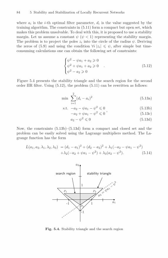
84 5 Stability and Stabilization of Locally Recurrent Networks
where ai is the i-th optimal filter parameter, di is the value suggested by thetraining algorithm. The constraints in (5.11) form a compact but open set, whichmakes this problem unsolvable. To deal with this, it is proposed to use a stabilitymargin. Let us assume a constant ψ (ψ < 1) representing the stability margin.The problem is to project the poles zi into the circle of the radius ψ. Derivingthe zeros of (5.9) and using the condition ∀i |zi| � ψ, after simple but time-consuming calculations one can obtain the following set of constraints:⎧⎪⎨
⎪⎩ψ2 − ψa1 + a2 � 0ψ2 + ψa1 + a2 � 0ψ2 − a2 � 0
. (5.12)
Figure 5.4 presents the stability triangle and the search region for the secondorder IIR filter. Using (5.12), the problem (5.11) can be rewritten as follows:
min2∑
i=1
(di − ai)2 (5.13a)
s.t. −a2 − ψa1 − ψ2 � 0 , (5.13b)−a2 + ψa1 − ψ2 � 0 (5.13c)a2 − ψ2 � 0 (5.13d)
Now, the constraints (5.13b)–(5.13d) form a compact and closed set and theproblem can be easily solved using the Lagrange multipliers method. The La-grange function has the form
L(a1, a2, λ1, λ2, λ3) = (d1 − a1)2 + (d2 − a2)2 + λ1(−a2 − ψa1 − ψ2)+λ2(−a2 + ψa1 − ψ2) + λ3(a2 − ψ2). (5.14)
a2
a1-1 1
-1
1
stability trianglesearch region
P3
P1 P2
a2=
ψa1− ψ
2
Fig. 5.4. Stability triangle and the search region

5.1 Stability Analysis – Networks with One Hidden Layer 85
Let us define the Kuhn-Tucker conditions:⎧⎪⎪⎪⎪⎪⎪⎪⎪⎪⎪⎪⎪⎪⎪⎪⎪⎪⎪⎨⎪⎪⎪⎪⎪⎪⎪⎪⎪⎪⎪⎪⎪⎪⎪⎪⎪⎪⎩
∂L
∂a1= −2d1 + 2a1 − ψλ1 + ψλ2 = 0
∂L
∂a2= −2d2 + 2a2 − λ1 − λ2 + λ3 = 0
λ1∂L
∂λ1= λ1(−a2 − ψa1 − ψ2) = 0
λ2∂L
∂λ2= λ2(−a2 + ψa1 − ψ2) = 0
λ3∂L
∂λ3= λ3(a2 − ψ2) = 0
∀i λi � 0
. (5.15)
The solution of (5.15) can be derived by analyzing which constraints will beactive in a specific case. There are six possibilities:
1. The constraint (5.13b) is active (λ1 �= 0, λ2 = 0, λ3 = 0), the correctedcoordinates are calculated using the formulae
a1 = d1 +ψ
1 + ψ2 (−d2 − ψd1 − ψ2),
a2 = d2 +1
1 + ψ2 (−d2 − ψd1 − ψ2);
2. The constraint (5.13c) is active (λ2 �= 0, λ1 = 0, λ3 = 0), the correctedcoordinates are obtained as follows:
a1 = d1 − ψ
1 + ψ2 (−d2 + ψd1 − ψ2),
a2 = d2 +1
1 + ψ2 (−d2 + ψd1 − ψ2);
3. The constraint (5.13d) is active (λ3 �= 0, λ1 = 0, λ2 = 0), the correctedparameters are a1 = d1, a2 = ψ2;
4. The constraints (5.13b) and (5.13d) are active (λ1 �= 0, λ3 �= 0, λ2 = 0), thesolution is the point P1 = (a1, a2) = (−2ψ, ψ2) (see Fig. 5.4);
5. The constraints (5.13c) and (5.13d) are active (λ2 �= 0, λ3 �= 0, λ1 = 0), thesolution is the point P2 = (a1, a2) = (2ψ, ψ2) (see Fig. 5.4);
6. The constraints (5.13b) and (5.13c) are active (λ1 �= 0, λ2 �= 0, λ3 = 0), thesolution is the point P3 = (a1, a2) = (0, −ψ2) (see Fig. 5.4).
The feasible region considered is defined in the form of a triangle. The possibilitythat all three constraints are active never holds in this case, because there doesnot exist such a point to violate all constraints simultaneously.
Table 5.2 presents the minimum distance projection algorithm. As one cansee, by using the solution of the Kuhn-Tucker conditions (5.15), a very simplealgorithm is obtained.

86 5 Stability and Stabilization of Locally Recurrent Networks
Table 5.2. Outline of the minimum distance projection
Step 0: Initiation
Choose θ0 ∈ Θ, set k := 0
Step 1: Compute g(θk) and update the parameter estimate θk+1
Step 2: Check constraint violation and correct the parameters according to
the solution of (5.15)
Step 3: Termination criteria
if (termination criterion satisfied) then STOP else go to Step 1
In the case when neurons consist of the first order filter, the lower and upperbounds have the following values: θi
l = −1, and θiu = 1. If a feedback parameter
θi exceeds the lower bound θil , then θi is set to the value −ψ. On the other hand,
if a feedback filter parameter θi exceeds the upper bound θiu, then θi is set to
the value ψ.This simple algorithm generates a new feasible solution which lies in a minimal
distance from the solution proposed by the training procedure and guaranteesthe stability of the filter, simultaneously deteriorating the training of the networkin a minimum way.
5.1.3 Strong Convergence
Both of the proposed algorithms are projection based methods and can be rep-resented in the following general form:
θk+1 = πG
[θk − akgk(θk)
], (5.16)
where πG : Rp → G is the projection onto the constraint set G. Introduce theprojection term zk; then (5.16) can be rewritten as
θk+1 = θk − akgk(θk) + akzk. (5.17)
In this way, akzk is the vector of shortest distance needed to take θk −akgk(θk)back to the constraint set G if it is not in G. As gk(θk) is the estimate of thegradient gk(θk), the bias in gk(θk) is defined as follows:
bk(θk) = E[gk(θk) − g(θk)|θk
], (5.18)
where E[·|·] denotes the conditional expectation. It is expected that bk → 0 ask → ∞. Using (5.18) and defining the error term
ek(θk) = gk(θk) − E[gk(θk)|θk
], (5.19)
one can rewrite (5.17) as
θk+1 = θk − akgk(θk) − akbk(θk) − akek(θk) + akzk. (5.20)

5.1 Stability Analysis – Networks with One Hidden Layer 87
All methods of convergence analysis need to show that the so-called “tail” effectof the noise vanishes. Such behaviour is essentially due to the martingale differ-ence property and decreasing the step size ak. Firstly, let us define sets describingthe feasible regions of the network parameters derived at the beginning of Sec-tion 5.1. The proposed projection algorithms work with inequality constraints.Let us introduce the following assumptions, where Assumption 1 defines a set ofconstraints when first order filters inside neurons are applied whilst Assumption2 defines a set of constraints in the case of second order filters.
Assumption 1. Define the set G = {θ : θil � θi � θi
u}, where θil < θi
u and θil and
θiu are real numbers. The set G is hyperrectangle in this case.
Assumption 2. Define the set G = {θ : qi(θ) � 0, i = 1, . . . , 3} and assume thatit is connected, compact and non-empty. Let qi(·), i = 1, . . . , 3 be continuouslydifferentiable real-valued functions.
Aditionally, it is needed to show that the fundamental algorithm (SPSA) isconvergent. Recall the following assumptions:
Assumption 3 (Gain sequences). ak, ck > 0 ∀k; ak → 0, ck → 0 as k → ∞;∑∞k=0 ak = ∞,
∑∞k=0
(ak
ck
)2< ∞.
Assumption 4 (Measurement noise). For some α0, α1, α2 > 0 and ∀k, E[ε(±)2
k ] �α0, E[J(θk ± Δk)2] � α1, and E[Δ−2
kl ] � α2 (l = 1, 2, . . . , p).
Assumption 5 (Iterate boundedness). ‖θk‖ < ∞ a.s. ∀k.
Assumption 6 (Relationship to Ordinary Differential Equations (ODE)). θ∗ isan asymptotically stable solution of the differential equation dx(t)/dt = −g(x).
Assumption 7. Let D(θ∗) = {x0 : limt→∞ x(t|x0) = θ∗}, where x(t|x0) denotesthe solution to the differential equation of Assumption 6 based on the initialconditions x0. There exists a compact set S ⊆ D(θ∗) such that θk ∈ S infinitelyoften for almost all sample points.
Assumption 8 (Smoothness of J). J is three-time continuously differentiable andbounded on R
p.
Assumption 9 (Statistical properties of perturbations). {Δki} are independentfor all k, i, identically distributed for all i at each k, symmetrically distributedabout zero and uniformly bounded in magnitude for all k, i.
For motivations and a detailed discussion about Assumptions 3–9 the readeris referred to [147, 145].
Proposition 5.2. Assume that the conditions of SPSA (Assumptions 3–9) holdfor the algorithm (5.16) with any of the constraint set conditions (Assumption1 or Assumption 2) holding. Then
θk → θ∗ as k → ∞ a.s. (w.p.1). (5.21)
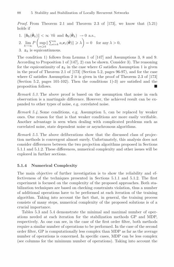
88 5 Stability and Stabilization of Locally Recurrent Networks
Proof. From Theorem 2.1 and Theorem 2.3 of [173], we know that (5.21)holds if
1. ‖bk(θk)‖ < ∞ ∀k and bk(θk) → 0 a.s.,
2. limk→∞
P
(supm�k
‖∑m
i=k aiei(θ)‖ � λ
)= 0 for any λ > 0,
3. zk is equicontinuous.
The condition 1) follows from Lemma 1 of [147] and Assumptions 3, 8 and 9.According to Proposition 1 of [147], 2) can be shown. Consider 3). The reasoningfor the equicontinuity of zk in the case where G satisfies Assumption 1 is givenin the proof of Theorem 2.1 of [173] (Section 5.2, pages 96-97), and for the casewhere G satisfies Assumption 2 it is given in the proof of Theorem 2.3 of [173](Section 5.2, pages 101-102). Then the conditions 1)-3) are satisfied and theproposition follows. �
Remark 5.3. The above proof is based on the assumption that noise in eachobservation is a martingale difference. However, the achieved result can be ex-panded to other types of noise, e.g. correlated noise.
Remark 5.4. Some conditions, e.g. Assumption 5, can be replaced by weakerones. One reason for that is that weaker conditions are more easily verifiable.Another advantage is seen when dealing with complicated problems such ascorrelated noise, state dependent noise or asynchronous algorithms.
Remark 5.5. The above deliberations show that the discussed class of projec-tion methods is convergent almost surely. Unfortunately, this analysis does notconsider differences between the two projection algorithms proposed in Sections5.1.1 and 5.1.2. These differences, numerical complexity and other issues will beexplored in further sections.
5.1.4 Numerical Complexity
The main objective of further investigation is to show the reliability and ef-fectiveness of the techniques presented in Sections 5.1.1 and 5.1.2. The firstexperiment is focused on the complexity of the proposed approaches. Both sta-bilization techniques are based on checking constraints violation, thus a numberof additional operations have to be performed at each iteration of the trainingalgorithm. Taking into account the fact that, in general, the training processconsists of many steps, numerical complexity of the proposed solutions is of acrucial importance.
Tables 5.3 and 5.4 demonstrate the minimal and maximal number of oper-ations needed at each iteration for the stabilization methods GP and MDP,respectively. As one can see, in the case of the first order filter, both methodsrequire a similar number of operations to be performed. In the case of the secondorder filter, GP is computationally less complex than MDP as far as the averagenumber of operations is concerned. In specific cases, MDP can be less complex(see columns for the minimum number of operations). Taking into account the

5.1 Stability Analysis – Networks with One Hidden Layer 89
Table 5.3. Number of operations: GP method
Type of operation first order filter second order filter
min max average min max average
statement checking 1 1 1 3 3 3
setting operations 1 2 1.5 2 5 3.5
additions 1 1 1 2 2 2
multiplications 1 1 1 2 2 2
TOTAL 4 5 4.5 9 12 10.5
Table 5.4. Number of operations: MDP method
Type of operation first order filter second order filter
min max average min max average
statement checking 1 2 1.5 2 3 2.5
setting operations 0 1 0.5 0 2 1
additions 0 2 1 0 16 8
multiplications 0 1 0.5 0 16 8
TOTAL 1 6 3.5 2 37 19.5
fact that the training procedure consists of hundreds of different kinds of oper-ations, it seems that the proposed solutions are very attractive because of theirsimplicity. The next experiment shows how time-consuming these methods are.
Let us consider the second order linear process discussed in Example 3.8. Thelearning data are generated by feeding a random signal of the uniform distribu-tion |u(k)| � (a2 + ω2) to the process and recording its output signal. In thisway, a training set containing 200 patterns is generated. In order to comparethe stabilization methods, a number of experiments were performed using a dif-ferent number of hidden neurons and a different number of learning steps. Allmethods are implemented in Borland C++ BuilderTM Enterprise Suite Ver. 5.0.Simulations are performed using a PC with a Celeron 600 processor and a 160MB RAM. Training using each method was performed 10 times and the averageresults are presented in Table 5.5. The results confirm that with a small numberof learning steps the differences between the methods are negligible, a few hun-dred of a second. Greater differences are observed in the case of a larger numberof iterations. As one can see in Table 5.5, after 15000 learning steps there are3,6 sec and 13,2 sec of difference between GP and training without stabiliza-tion and MDP and training without stabilization, respectively. The results showthat the proposed methods are very simple as far as software implementation isconcerned, and they do not prolong learning in a significant way.

90 5 Stability and Stabilization of Locally Recurrent Networks
Table 5.5. Comparison of the learning time for different methods
CharacteristicsStabilization method
none GP MDP
v = 3, r = 2, nmax = 500 7.44 sec 7.46 sec 7.47 sec
v = 8, r = 2, nmax = 500 12.59 sec 12.65 sec 12,7 sec
v = 15, r = 2, nmax = 500 25.16 sec 25.18 sec 25.18 sec
v = 7, r = 2, nmax = 5000 1.98 min 1.99 min 1.99 min
v = 7, r = 2, nmax = 15000 6.93 min 6.99 min 7.15 min
5.1.5 Pole Placement
To show stabilization capabilities of the proposed methods, several experimentsare carried out. The first one is the identification of a dynamic process withoutthe stabilization of the learning. In the next two experiments, to train the dy-namic network the GP and MDP techniques are applied. All experiments areperformed with exactly the same learning data, initial network parameters andparameters of the training algorithm. The process to be identified is describedby the following difference equation [20]:
yd(k) =yd(k − 1)
1 + y2d(k − 2)
+ u3(k − 3). (5.22)
This is a third order dynamic process. To identify (5.22), the dynamic network(3.39) is applied. The arbitrarily selected two-layer architecture contains fourhidden dynamic neurons with second order IIR filters and hyperbolic tangentactivation functions, and one linear output neuron. The training process wascarried out off-line for 500 iterations using a pseudo-random input uniformlydistributed on the interval [-2,2]. The parameters of SPSA are as follows: A = 0,α = 0.2, γ = 0.1, a = 0.0002, c = 0.001.
0 50 100 150 200 250 300 350 400 45010
3
104
Epoch
Sum
-square
derr
or
Fig. 5.5. Sum squared error – training without stabilization

5.1 Stability Analysis – Networks with One Hidden Layer 91
(a) (b)
(c) (d)Re(z) Re(z)
Re(z) Re(z)
Im
(z)
Im
(z)
Im
(z)
Im
(z)
-1
0
1
-1 0 1
-1
0
-1 0 1
1
unstablepole
unstablepole
unstablepole
unstablepole
unstablepole
-1
0
-1 0 1
1
-1
0
-1 0 1
1
Fig. 5.6. Poles location during learning without stabilization: neuron 1 (a), neuron 2(b), neuron 3 (c), neuron 4 (d)
Figure 5.5 presents the learning error of the neural network in the case whenconstraints on the network parameters are not applied. As one can see there,the course of the error is not smooth. There are great fluctuations caused by theinstability of the neurons, including the large jump after the 400-th iteration.Poles placement during learning without stabilization is shown in Fig. 5.6. To
clarify the analysis, poles placement after 20 algorithm iterations is presentedonly. Three out of four neurons lost stability. Only the poles of the third neuron(Fig. 5.6(c)) are inside the unit circle. In turn, Fig. 5.7 presents poles locationin the case when the GP approach is applied. As one can observe, each neuronkeeps its own poles inside the unit circle. Unstable poles from the previous caseare corrected according to GP to fall into a stable region. At each iterationthe entire neural model is stable and the convergence of the learning is faster.Interesting results can be observed by analysing Figs. 5.6(c) and 5.7(c). In thecase when the poles are stable, the stabilization method does not change poleslocation and, consequently, does not introduce any needless operations. A crucialfactor for the correct work of the GP method is the initial poles location. The
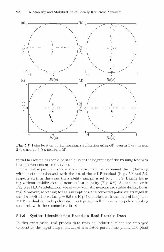
92 5 Stability and Stabilization of Locally Recurrent Networks
(a) (b)
(c) (d)Re(z) Re(z)
Re(z) Re(z)
Im
(z)
Im
(z)
Im
(z)
Im
(z)
-1
0
-1 0 1
1
-1
0
1
-1 0 1
-1
0
1
-1 0 1-1
0
1
-1 0 1
Fig. 5.7. Poles location during learning, stabilization using GP: neuron 1 (a), neuron2 (b), neuron 3 (c), neuron 4 (d)
initial neuron poles should be stable, so at the beginning of the training feedbackfilter parameters are set to zero.
The next experiment shows a comparison of pole placement during learningwithout stabilization and with the use of the MDP method (Figs. 5.8 and 5.9,respectively). In this case, the stability margin is set to ψ = 0.9. During learn-ing without stabilization all neurons lost stability (Fig. 5.8). As one can see inFig. 5.9, MDP stabilization works very well. All neurons are stable during learn-ing. Moreover, according to the assumptions, the corrected poles are arranged inthe circle with the radius ψ = 0.9 (in Fig. 5.9 marked with the dashed line). TheMDP method controls poles placement pretty well. There is no pole exceedingthe circle with the assumed radius ψ.
5.1.6 System Identification Based on Real Process Data
In this experiment, real process data from an industrial plant are employedto identify the input-output model of a selected part of the plant. The plant

5.1 Stability Analysis – Networks with One Hidden Layer 93
(a) (b)
(c) (d)Re(z) Re(z)
Re(z) Re(z)
Im
(z)
Im
(z)
Im
(z)
Im
(z)
-1
0
-1 0 1
1
unstablepole
-1
0
-1 0 1
1
unstablepoles
-1
0
1 20-2 -1
1
unstablepole
unstablepole
-1
0
-1-2 0 1
1
unstablepole
unstablepole
unstablepole
Fig. 5.8. Poles location during learning without stabilization: neuron 1 (a), neuron 2(b), neuron 3 (c), neuron 4 (d)
considered is a sugar actuator described in detail in Section 8. The data usedfor the learning and testing sets were suitably preprocessed removing trends,resulting in the 500-th and 1000-th elements for the learning and testing datasets, respectively. To model the process (8.4), the dynamic neural network (3.39)is applied using three hidden neurons, each including a second order IIR filter anda hyperbolic tangent activation function. The parameters of the SPSA algorithmare A = 0, α = 0.35, γ = 0.1, a = 0.001, c = 0.01. As a stabilization method,the MDP technique is applied with the stability margin ψ = 0.9. The responsesof the neural model obtained for both the learning and testing data sets arepresented in Fig. 5.10. The mean squared output error for the learning set isequal to 1.5523, and for the testing set – 7.6094.
5.1.7 Convergence of Network States
The last experiment aims at showing the convergence of the states of the networktrained without and with stabilization techniques. The training data and the

94 5 Stability and Stabilization of Locally Recurrent Networks
(a) (b)
(c) (d)Re(z) Re(z)
Re(z) Re(z)
Im
(z)
Im
(z)
Im
(z)
Im
(z)
-1
0
-1 0 1
1
-1
0
-1 0 1
1
-1
0
-1 0 1
1
-1
0
-1 0 1
1
Fig. 5.9. Poles location during learning, stabilization using MDP: neuron 1 (a), neuron2 (b), neuron 3 (c), neuron 4 (d)
(a) (b)
0 50 100 150 200 250 300 350 400 450-30
-20
-10
0
10
20
30
Time
Outp
uts
0 100 200 300 400 500 600 700 800 900-15
-10
-5
0
5
10
15
20
25
30
35
Time
Outp
uts
Fig. 5.10. Actuator (solid line) and model (dashed line) outputs for learning (a) andtesting (b) data sets

5.1 Stability Analysis – Networks with One Hidden Layer 95
(a) (b)
0 100 200 300 400 500 600 700 800 90010
-1
100
101
102
103
Epoch
Sum
-square
derr
or
1 2 3 4 5Time
Netw
ork
sta
tes
6 7 8 9 10
-15
-10
-5
0
5
10
15
20
Fig. 5.11. Results of training without stabilization: error curve (a) and the convergenceof the state x(k) of the neural model (b)
(a) (b)
0 100 200 300 400 500 600 700 800 900Epoch
100
101
102
Sum
-square
derr
or
0 5 10 15 20 25 30-2
-1
0
1
Netw
ork
sta
tes
Time
Fig. 5.12. Results of training with GP: error curve (a) and the convergence of thestate x(k) of the neural model (b)
structure of the network are the same as in the previous experiment. Here, theparameters of SPSA are as follows: A = 100, α = 0.602, γ = 0.1, a = 0.015,c = 0.1. Figure 5.11 presents the training results of the basic algorithm withoutstabilization. As one can see, the error curve is convergent. In spite of that,the neural model is not stable, because four out of six states are divergent.Consequently, two out of three neurons go into saturation and dynamic as wellas approximation properties of the neural network are strongly restricted. Thisexample shows clearly that the stabilization problem is important and necessaryto tackle during training. The next two figures (Figs. 5.12 and 5.13) show theresults of training when a stabilization technique is used. Both of the proposedmethods assure the stability of the neural model. Neural states are convergent,as depicted in Fig. 5.12 for the GP algorithm and in Fig. 5.13 in the case ofMDP.
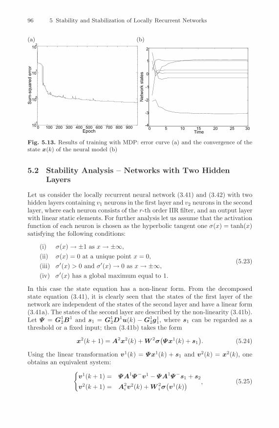
96 5 Stability and Stabilization of Locally Recurrent Networks
(a) (b)
0 100 200 300 400 500 600 700 800 900Epoch
10-1
100
101
102
Sum
-square
derr
or
0 5 10 15 20 25 30-4
-3
-2
-1
0
1
2
Time
Netw
ork
sta
tes
Fig. 5.13. Results of training with MDP: error curve (a) and the convergence of thestate x(k) of the neural model (b)
5.2 Stability Analysis – Networks with Two HiddenLayers
Let us consider the locally recurrent neural network (3.41) and (3.42) with twohidden layers containing v1 neurons in the first layer and v2 neurons in the secondlayer, where each neuron consists of the r-th order IIR filter, and an output layerwith linear static elements. For further analysis let us assume that the activationfunction of each neuron is chosen as the hyperbolic tangent one σ(x) = tanh(x)satisfying the following conditions:
(i) σ(x) → ±1 as x → ±∞,
(ii) σ(x) = 0 at a unique point x = 0,
(iii) σ′(x) > 0 and σ′(x) → 0 as x → ±∞,
(iv) σ′(x) has a global maximum equal to 1.
(5.23)
In this case the state equation has a non-linear form. From the decomposedstate equation (3.41), it is clearly seen that the states of the first layer of thenetwork are independent of the states of the second layer and have a linear form(3.41a). The states of the second layer are described by the non-linearity (3.41b).Let Ψ = G1
2B1 and s1 = G1
2D1u(k) − G1
2g11, where s1 can be regarded as a
threshold or a fixed input; then (3.41b) takes the form
x2(k + 1) = A2x2(k) + W 2σ(Ψx1(k) + s1
). (5.24)
Using the linear transformation v1(k) = Ψx1(k) + s1 and v2(k) = x2(k), oneobtains an equivalent system:{
v1(k + 1) = ΨA1Ψ−v1 − ΨA1Ψ−s1 + s2,
v2(k + 1) = A2i v
2(k) + W 2i σ
(v1(k)
) (5.25)

5.2 Stability Analysis – Networks with Two Hidden Layers 97
where Ψ− is a pseudoinverse of the matrix Ψ (e.g. in a Moore-Penrose sense),and s2 = ΨW 1u(k)+s1 is a threshold or a fixed input. Let v∗ = [v1∗v2∗]T be anequilibrium point of (5.25). Introducing an equivalent coordinate transformationz(k) = v(k) − v∗(k), the system (5.25) can be transformed to the form{
z1(k + 1) = ΨA1Ψ−z1(k)z2(k + 1) = A2z2(k) + W 2f (z1(k))
, (5.26)
where f(z1(k)) = σ(z1(k) + v1∗(k)) − σ(v1∗(k)). Substituting z(k) = [z1(k)z2(k)]T , one finally obtains
z(k + 1) = Az(k) + Wf(z(k)), (5.27)
where
A =[
ΨA1Ψ− 00 A2
], W =
[0 0
W 2 0
]. (5.28)
5.2.1 Second Method of Lyapunov
In this section, the second method of Lyapunov is used to determine stabilityconditions for the system (5.27).
Lemma 5.6 (Global stability theorem of Lyapunov [77]). Let x = 0 bean equilibrium point of the system
x(k + 1) = f(x(k)), (5.29)
and V : Rn → R a continuously differentiable function such that
1. V (x(k) = 0) = 0,2. V (x(k)) > 0, for x �= 0,3. V (x) → ∞ for ‖x‖ → ∞,4. ΔV (x(k)) = V (x(k + 1)) − V (x(k)) < 0 for x �= 0.
Then, the equilibrium point x = 0 is globally asymptotically stable and V (x) isa global Lyapunov function.
Theorem 5.7. The neural system represented by (5.27) is globally asymptoti-cally stable if the following condition is satisfied:
‖A‖ + ‖W‖ < 1. (5.30)
Proof. Let V (z) = ‖z‖ be a Lyapunov function for the system (5.27). Thisfunction is positive definite with the minimum at x(k) = 0. The difference alongthe trajectory of the system is given as follows:
ΔV (z(k)) = ‖z(k + 1)‖ − ‖z(k)‖= ‖Az(k) + Wf(z(k))‖ − ‖z(k)‖� ‖Az(k)‖ + ‖Wf(z(k))‖ − ‖z(k)‖.
(5.31)
98 5 Stability and Stabilization of Locally Recurrent Networks
The activation function σ is a short map with the Lipschitz constant L = 1.Then f is also a short map, with the property ‖f(z(k))‖ � ‖z(k)‖, and (5.31)can be expressed in the form
ΔV (z(k)) � ‖A‖‖z(k)‖ + ‖W‖‖z(k)‖ − ‖z(k)‖� (‖A‖ + ‖W‖ − 1) ‖z(k)‖.
(5.32)
From (5.32) one can see that if
‖A‖ + ‖W‖ < 1, (5.33)
then ΔV (z(k)) is negative definite and the system (5.27) is globally asymptoti-cally stable, which completes the proof. �Remark 5.8. The theorem formulates the sufficient condition only, not a neces-sary one. Therefore, if the condition (5.30) is not satisfied, one cannot judge thestability of the system.
Remark 5.9. The condition (5.30) is very restrictive. The matrix A is a blockdiagonal one with the entries ΨA1Ψ− and A2
i , for i = 1, . . . , v2. For blockdiagonal matrices, the following relation holds:
‖A‖ = maxi=1,...,n
{‖Ai‖} . (5.34)
The entries of A for i = 2, . . . , v2 have the form (3.19). For such matrices, thenorm is greater than or equal to one. Thus, Theorem 5.7 is useless, because thereis no network (5.27) able to satisfy (5.30). One way to make (5.30) applicable tothe system (5.27) is to use the modified neuron state matrix of the form (3.24)with the parameter ν. The parameter ν can be selected experimentally by theuser or can be adapted by a training procedure.
Remark 5.10. In spite of its shortcomings, the condition (5.30) is very attractivebecause of its simplicity and ease of use.
Remark 5.11. The theorem is also valid for other activation functions with theLipschitz constant L � 1, satisfying the conditions (5.23).
Example 5.12. Consider the neural network described by (3.41) and (3.42) with7 neurons in the first hidden layer and 4 neurons in the second hidden layer.Each neuron consists of the second order IIR filter and a hyperbolic tangentactivation function. The network is applied to model the process (5.1). Trainingwas carried out for 5000 steps using the SPSA algorithm with the settings a =0.002, c = 0.01, α = 0.302, γ = 0.101, A = 100. The training set consists of 100samples generated randomly using the uniform distribution. The sum of squarederrors for the training set is 0.6943, and for the testing set containing another100 samples it is 1.2484. The stability of the trained network was tested usingthe norm stability condition (5.30) as follows:
‖A‖2 + ‖W‖2 = 4.0399 > 1 (5.35)‖A‖1 + ‖W‖1 = 4.7221 > 1 , (5.36)
‖A‖∞ + ‖W‖∞ = 6.4021 > 1 (5.37)

5.2 Stability Analysis – Networks with Two Hidden Layers 99
(a) (b)
0 20 40 60 80 100−1.5
−1
−0.5
0
0.5
1
1.5
x1
Time0 20 40 60 80 100
−3
−2
−1
0
1
2
3
Time
x2
(c) (d)
0 5 10 15 20−0.8
−0.6
−0.4
−0.2
0
0.2
0.4
0.6
0.8
1
Time
z1
0 5 10 15 20−1.5
−1
−0.5
0
0.5
1
1.5
Time
z2
(e)
0 1000 2000 3000 400010
−1
100
101
102
Epoch
Sum
−sq
uare
d er
ror
Fig. 5.14. Convergence of network states: original system (a)–(b), transformed system(c)–(d), learning track (e)

100 5 Stability and Stabilization of Locally Recurrent Networks
where
‖X‖2 =√
λmaxXT X
‖X‖1 = max1�i�n
n∑j=1
|xij | .
‖X‖∞ = max1�j�n
n∑i=1
|xij |
Unfortunately, based on (5.35)–(5.37), the norm stability condition cannot judgethe stability of the system. On the other hand, observing the convergence ofthe network states one can see that the system is stable. Figures 5.14(a) and(b) present the convergence of the states of the first and second layers of thesystem (3.41). In turn, in Figs 5.14(c) and (d) the convergence of the transformedautonomous system (5.27) is shown. All states converge to zero, which meansthat the network is stable.
This experiment clearly shows that the norm stability condition is very restric-tive. Moreover, to satisfy the condition (5.30) the entries of both matrices A andW should have relatively small values. The following procedure proposes thetraining of the network assuring the stability of the model. Assuming that eachneuron in the network is represented by the modified state transition matrix(3.24), the norm of the matrix W is checked after each training step. If the normstability condition is not satisfied, the entries of W are decreased iteratively.
Example 5.13. Le us revisit the problem considered in the example 5.12, butthis time with each neuron in the network represented by the modified statetransition matrix (3.24) with the parameter ν = 0.5. The training is carriedout using the procedure shown in Table 5.6. In this case, the sum of squarederrors for the training set is 0.7008, and for the testing set containing another
Table 5.6. Outline of norm stability checking
Step 0: Initiation
Choose the network parameters is such a way that ‖A‖ < 1, set ν < 1
Step 1: Update the network parameters using a training algorithm
Step 2: Assure the stability of the network
set x := 1;
while (‖A‖ + ‖W‖ > 1) dox := x + 1;
W := W/(x · ‖W‖);end while
Step 3: Termination criteria
if (termination criterion satisfied) then STOP else go to Step 1
5.2 Stability Analysis – Networks with Two Hidden Layers 101
100 samples it is 1.2924. The stability of the already trained network was testedusing the norm stability condition (5.30) as follows:
‖A‖2 + ‖W‖2 = 0.9822 < 1. (5.38)
In this case, the criterion is satisfied and the neural network is globally asymptot-ically stable. Similarly as in the previous example, Figs 5.15(a) and (b) presentthe convergence of the states of the first and second layers of the system (3.41).In turn, in Figs 5.15(c) and (d) the convergence of the transformed autonomoussystem (5.27) is shown. All states converge to zero, which means that the net-work is stable. The procedure presented in Table 5.6 guarantees the stabilityof the model. Recalculating the weights W can introduce perturbations to thetraining in the form of spikes, as illustrated in Fig. 5.15(e), but the training is,in general, convergent.
The discussed examples show that the norm stability condition is a restrictiveone. In order to successfully apply this criterion to network training, severalmodifications are required. Firstly, the form of the state transition matrix Ais modified and, secondly, the update of the network weight matrix W shouldbe performed during training. In the further part of the section less restrictivestability conditions are investigated.
Theorem 5.14. The neural system (5.27) is globally asymptotically stable ifthere exists a matrix P 0 such that the following condition is satisfied:
(A + W)T P (A + W) − P ≺ 0. (5.39)
Proof. Let us consider a positive definite candidate Lyapunov function:
V (z) = zT Pz. (5.40)
The difference along the trajectory of the system (5.27) is given as follows:
ΔV (z(k)) =V (z(k + 1)) − V (z(k))
= (Az(k) + Wf(z(k)))T P (Az(k) + Wf(z(k)))
− zT (k)P z(k)
=zT (k)AT PAz(k) + fT (z(k))WT PAz(k)
+ zT (k)AT PWf (z(k)) + fT (z(k))WT PWf(z(k))
− zT (k)P z(k).
(5.41)
For activation functions satisfying the conditions (5.23) it holds that |f(z)| � |z|and
f =
{f z > 0−f z < 0
; (5.42)
thenfT (z(k))WT P Az(k) � zT (k)WT PAz(k) (5.43)
zT (k)AT PWf(z(k)) � zT (k)AT P Wz(k) (5.44)

102 5 Stability and Stabilization of Locally Recurrent Networks
(a) (b)
0 20 40 60 80 100−1.5
−1
−0.5
0
0.5
1
Time
x1
0 20 40 60 80 100−0.4
−0.3
−0.2
−0.1
0
0.1
0.2
0.3
Time
x2
(c) (d)
0 5 10 15 20−1
−0.5
0
0.5
1
Time
z1
0 5 10 15 20−1
−0.5
0
0.5
1
Time
z2
(e)
0 1000 2000 3000 400010
−1
100
101
102
Epoch
Sum
−sq
uare
d er
ror
Fig. 5.15. Convergence of network states: original system (a)–(b), transformed system(c)–(d), learning track (e)

5.2 Stability Analysis – Networks with Two Hidden Layers 103
andfT (z(k))WT PWf(z(k)) � zT (k)WT PWz(k). (5.45)
Substituting the inequalities (5.43), (5.44) and (5.45) into (5.41), one obtains
ΔV (z(k)) �zT (k)AT P Az(k) + zT (k)WT PAz(k)
+ zT (k)AT PWz(k) + zT (k)WT PWz(k)
− zT (k)Pz(k)
�zT (k)(AT PA + WT PA + AT P W + WT PW − P )z(k)
�zT (k)((A + W)T P (A + W) − P
)z(k).
(5.46)
From (5.46) one can see that if
(A + W)T P (A + W) − P ≺ 0, (5.47)
then ΔV (z(k)) is negative definite and the system (5.27) is globally asymptoti-cally stable. �
Remark 5.15. From the practical point of view, the selection of a proper matrixP , in order to satisfy the condition (5.39), can be troublesome. Therefore, thecorollary presented below allows us to verify the stability of the system in aneasier manner. The corollary is formulated in the form of the Linear MatrixInequality (LMI). Recently, LMI methods have become quite popular amongresearchers from the control community due to their simplicity and effectivenesstaking into account numerical complexity [174].
Lemma 5.16 (Schur complement [175]). Let A ∈ Rn×n and C ∈ R
m×m besymmetric matrices, and A 0; then
C + BT A−1B ≺ 0, (5.48)
iff
U =[
−A B
BT C
]≺ 0 or, equivalently, U =
[C BT
B −A
]≺ 0. (5.49)
Corollary 5.17. The neural system (5.27) is globally asymptotically stable ifthere exists a matrix Q 0 such that the following LMI holds:[
−Q (A + W)Q
Q (A + W)T −Q
]≺ 0. (5.50)
Proof. From Theorem 5.14 one knows that the system (5.27) is globally asymp-totically stable if the following condition is satisfied:
(A + W)T P (A + W) − P ≺ 0. (5.51)
104 5 Stability and Stabilization of Locally Recurrent Networks
Applying the Schur complement formula to (5.51) yields[−P−1 A + W
(A + W)T −P
]≺ 0. (5.52)
In order to transform (5.52) into the LMI, let us introduce the substitutionQ = P−1 and then multiply the result from the left and the right by diag(I, Q)to obtain [
−Q (A + W)Q
Q (A + W)T −Q
]≺ 0.
�
Remark 5.18. The LMI (5.50) defines the so-called feasibility problem [175, 174].This convex optimisation problem can be solved effectively using poly-nomial-time algorithms, e.g. interior point methods. Interior point algorithms are com-putationally efficient and nowadays widely used for solving LMIs.
Example 5.19. Consider again the problem presented in Example 5.12. As isshown in that example, the norm stability condition cannot ensure the stabilityof the neural model (3.41). In this example, the condition given in Corollary5.17 is used to check the stability of the neural network. The problem was solvedwith the LMI solver implemented in the LMI Control Toolbox under Matlab7.0. After 4 iterations the solver found the feasible solution represented by thefollowing positive definite matrix Q:
Q=
⎡⎢⎢⎢⎢⎢⎢⎢⎢⎢⎢⎢⎢⎢⎢⎢⎢⎢⎢⎢⎢⎢⎢⎢⎢⎢⎣
48.6 0.1 −1.9 17.4 11.0 11.9 −14.9 −9.9 −8.9 −2.5 −1.4 2.4 1.3 −6.2 −2.10.1 82.9 −3.4 −9.9 20.5 19.4 −5.5 −0.5 1.1 6.9 −0.3 −0.7 0.9 0.4 −3.4−2.0 −3.4 30.8 0.6 4.6 −16.7 −7.2 5.7 9.0 1.3 0.8 13.1 7.2 0.9 −0.0117.4 −9.9 0.6 65.7 −14.9 −9.6 −26.0 2.3 8.2 −0.7 −0.3 −4.5 −2.4 4.0 −1.411.0 20.5 4.6 −14.9 56.1 −11.9 21.1 −7.1 6.4 −3.4 0.3 1.5 −1.5 1.8 −1.712.0 19.4 −16.7 −9.6 −11.7 77.3 −17.5 1.1 4.3 0.5 0.1 −2.6 −0.9 −7.4 2.6−14.9 −5.5 −7.2 −26.0 21.1 −17.5 51.5 −2.4 3.4 2.2 0.3 −1.9 −1.4 4.1 3.7−9.9 −0.5 5.7 2.3 −7.1 1.1 −2.4 123.9 23.3 6.2 2.2 −5.5 2.9 −1.3 1.9−8.9 1.1 9.0 8.2 6.4 4.3 3.4 23.3 185.4 1.6 4.9 3.1 −4.5 0.3 −0.1−2.5 6.9 1.3 −0.7 −3.4 0.5 2.2 6.2 1.6 122.5 10.3 −5.3 0.2 9.9 7.4−1.4 −0.3 0.8 −0.3 0.3 0.1 0.3 2.2 4.9 10.3 184.9 5.4 −3.3 −2.8 7.22.4 −0.7 13.1 −4.5 1.5 −2.6 −1.9 −5.5 3.1 −5.3 5.3 120.1 7.2 −8.6 −3.41.2 0.9 7.2 −2.4 −1.5 −0.9 −1.4 2.9 −4.5 0.2 −3.3 7.2 183.1 −5.4 −6.1−6.2 0.4 0.9 4.0 1.8 −7.4 −4.1 −1.3 0.3 9.9 −2.8 −8.6 −5.4 115.2 −0.2−2.1 −3.4 −0.01 −1.4 −1.7 2.6 3.7 1.9 −0.1 7.4 7.2 −3.4 −6.1 −0.2 178.9
⎤⎥⎥⎥⎥⎥⎥⎥⎥⎥⎥⎥⎥⎥⎥⎥⎥⎥⎥⎥⎥⎥⎥⎥⎥⎥⎦
.
For the matrix Q, the condition (5.50) is satisfied and the neural network is glob-ally asymptotically stable. This example shows that the condition presented inTheorem 5.14 is less restrictive than the norm stability condition. Moreover, rep-resenting a stability condition in the form of LMIs renders it possible to easilycheck the stability of the neural system.
Lemma 5.20 ([176, 177]). Let A ∈ Rq×q be a symmetric matrix, and P ∈
Rr×q and Q ∈ R
s×q real matrices; then there exists a matrix B ∈ Rr×s such
thatA + P T BT Q + QT BP ≺ 0 (5.53)

5.2 Stability Analysis – Networks with Two Hidden Layers 105
iff the inequalities W TP AW P ≺ 0 and W T
QAW Q ≺ 0 both hold, where W P ,and W Q are full rank matrices satisfying Im(W P ) = ker(P ) and Im(W Q) =ker(Q).
Example 5.21. The term (5.50) can be rewritten as
[−Q (A + W)Q
Q (A + W)T −Q
]=
[−Q AQ
QAT −Q
]+[
W
0
]Q
[0 I
]+
[0I
]QT
[W T 0
].
(5.54)Using Lemma 5.20 one obtains
W TP
[−Q AQ
QAT −Q
]W P ≺ 0, W T
Q
[−Q AQ
QAT −Q
]W Q ≺ 0, (5.55)
where W P = diag(ker(W ), I) and W Q = diag(I,0). Multiplying the secondinequality in (5.55) gives Q 0. Then (5.55) can be rewritten as
W TP RW P ≺ 0, Q 0, (5.56)
where
R =[
−Q AQ
QAT −Q
]. (5.57)
These LMI conditions can be solved with a less computational burden than theLMI condition 5.50. The results of computations, for different network structures,are presented in Table 5.7. The experiments were performed using the LMIControl Toolbox under Matlab 7.0 on a PC with Intel Centrino 1.4 GHz and a512MB RAM.
Lemma 5.20 is frequently used to reduce the number of matrix variables. Sincesome variables can be eliminated, the computational burden can be significantlyreduced. As shown in Table 5.7, the transformed LMIs (5.56) are relatively easierto solve than the LMIs (5.50). For each network structure considered, the LMIs(5.56) are solved performing one step of an algorithm only whilst the LMIs(5.50) require three or four steps. As a result, the LMIs (5.56) are solved 3–5times faster (Table 5.7).
Table 5.7. Comparison of methods
Network LMI (5.50) LMIs (5.56)
structure time [sec] iterations time [sec] iterations
7-4 0.0845 4 0.0172 1
15-7 0.545 3 0.189 1
25-10 6.5 4 1.7 1

106 5 Stability and Stabilization of Locally Recurrent Networks
5.2.2 First Method of Lyapunov
Theorems based on Lyapunov’s second method formulate sufficient conditionsfor global asymptotical stability of the system. In many cases, however, there is aneed to determine neccessary conditions. In such cases, Lyapunov’s first methodcan be used. Moreover, stability criteria developed using the second method ofLyapunov cannot be used as a starting point to determime constraints on thenetwork parameters. Thus, the optimisation problem with constraints cannotbe determined. This section presents an approach, based on the first method ofLyapunov, which allows us to elaborate a training procedure with constraints onthe network parameters. Thus, the training process can guarantee the stabilityof the neural model.
Lemma 5.22 (Lyapunov’s first method). Let x∗ = 0 be an equilibrium pointof the system
x(k + 1) = f(x(k)), (5.58)
where f : D → Rn is a continuously differentiable function and D is a neigh-
bourhood of the origin. Define the Jacobian of (5.58) in the neigbourhood of theequilibrium point x∗ = 0 as
J =∂f
∂x |x=0. (5.59)
Then
1. The origin is locally asymptotically stable if all the eigenvalues of J areinside the unit circle in the complex plane.
2. The origin is unstable if one or more of the eigenvalues of J are outside theunit circle in the complex plane.
Theorem 5.23. The neural system (5.27) composed of neurons with first orderfilters (r = 1) is locally asymptotically stable if the following conditions aresatisfied:
1. |a11i| < 1 ∀i = 1, . . . , v1, and |a2
1i| < 1 ∀i = 1, . . . , v2,2. b1
1i �= 0 ∀i = 1, . . . , v1.
Proof. The Jacobian of (5.27) is given by
J =[
ΨA1Ψ− 0W 2f ′(0) A2.
]. (5.60)
The characteristic equation has the form
det(J − λI) = 0. (5.61)
The Jacobian is the block matrix and then the determinant of J − λI isgiven by
det(J − λI) = (ΨA1Ψ− − λ)(A2 − λ) − W 2σ′(0) · 0.
= (ΨA1Ψ− − λ)(A2 − λ)(5.62)

5.2 Stability Analysis – Networks with Two Hidden Layers 107
Finally, the characteristic equation receives the form
(ΨA1Ψ− − λ)(A2 − λ) = 0, (5.63)
and the system is stable if all eigenvalues of both matrices ΨA1Ψ− and A2
are located in the unit circle. In our case, A1 = diag(a11, . . . , a
1v1
), A2 =diag(a2
1, . . . , a2v2
) and B1 = diag(b11, . . . , b
1v1
). If Condition 2 is satisfied, thenΨ = diag(g1
21b11, . . . , g
12v1
b1v1
). In this trivial case, a pseudoinverse of Ψ is givenas follows:
Ψ− =
⎡⎢⎢⎢⎢⎢⎢⎢⎢⎣
1g121
b11
. . . 0
.... . .
...
0 . . .1
g12v1
b1v1
⎤⎥⎥⎥⎥⎥⎥⎥⎥⎦
(5.64)
and, finally, ΨA1Ψ− = A1. Then the system is stable if all eigenvalues of A1 andA2 are located in the unit circle. Taking into account the reasoning presentedin Section 5.1, one knows that all eigenvalues of a block diagonal matrix arelocated in the unit circle if the eigenvalues of each matrix on the diagonal arelocated in the unit circle. According to this, |a1
1i| < 1, ∀i = 1, . . . , v1 and|a2
1i| < 1, ∀i = 1, . . . , v2, which completes the proof. �
Theorem 5.24. The neural system (5.27) composed of neurons with second or-der filters (r = 2) is locally asymptotically stable if the following conditions aresatisfied:
1. For each entry of A1 and A2, a set of inequalities is satisfied:⎧⎪⎨⎪⎩
1 − a1 + a2 > 01 + a1 + a2 > 01 − a2 > 0
; (5.65)
2. (b11i)
2 + (b12i)
2 �= 0 ∀i = 1, . . . , v1;3. |b1
1i| < |b12i| ∀i = 1, . . . , v1.
Proof. From the proof of Theorem 5.23 one knows that the system (5.27) isstable if the eigenvalues of ΨA1Ψ− and A2 are located in the unit circle. Letus consider the eigenvalues of A2 first. According to the reasoning presented inSection 5.1, one knows that the eigenvalues of A2 are stable if for each entry onthe diagonal a set of inequalities (5.65) holds. Next, take into account ΨA1Ψ−.This is a block diagonal matrix with the entries Ψ iA
1i Ψ
−i , i = 1, . . . , v1, where
Ψ i = g12ib
1i . Using Singular Value Decomposition (SVD), it is easy to verify that
Ψ−i =
b1i
g12i‖b1
i ‖22, (5.66)

108 5 Stability and Stabilization of Locally Recurrent Networks
where ‖x‖2 is the Euclidean norm of the vector x. Using (5.66), Ψ iA1i Ψ
−i can
be represented as
Ψ iA1i Ψ
−i =
−a11i(b
11i)
2 + b11ib
12i(1 − a1
2i)(b1
1i)2 + (b12i)2
. (5.67)
In order to obtain a stable system, the condition∣∣∣∣−a11i(b
11i)
2 + b11ib
12i(1 − a1
2i)(b1
1i)2 + (b12i)2
∣∣∣∣ < 1, ∀i = 1, . . . , v1 (5.68)
should be satisfied. To clarify the presentation in the following deliberations, theindex i is omitted. Let us rewrite (5.68) as follows:
−(b11)
2 − (b12)
2 − b11b
12 < f(a1
1, a12) < (b1
1)2 + (b1
2)2 − b1
1b12, (5.69)
where f(a11, a
12) = −a1
1(b11)
2 − a12b
11b
12. To complete the proof, it is necessary to
show thatmax f(a1
1, a12) < (b1
1)2 + (b1
2)2 − b1
1b12
andmin f(a1
1, a12) > −(b1
1)2 − (b1
2)2 − b1
1b12.
Therefore, it is required to solve two optimisation problems:
max f(a11, a
12)
s.t. 1 − a1 + a2 � 01 + a1 + a2 � 01 − a2 � 0
and
min f(a11, a
12)
s.t. 1 − a1 + a2 � 0 .1 + a1 + a2 � 01 − a2 � 0
(5.70)
The graphical solution of the optimisation problems (5.70) is presented inFig. 5.16.
Case 1. b1b2 > 0 and b21 > b1b2. The course of the cost function is presented in
Fig. 5.16(a). The maximum is located at the point P1 = (−2, 1) and the mini-mum at the point P2(2, 1).
Case 2. b1b2 > 0 and b21 < b1b2. The course of the cost function is presented in
Fig. 5.16(b). The maximum is located at the point P3 = (0, 1) and the minimumat the point P2(2, 1).
There is another posibility, when b1b2 > 0 and b21 = b1b2, but in this case
b1 = b2 and Condition 3 is not satisfied.
Case 3. b1b2 < 0 then b21 > b1b2. The course of the cost function is presented
in Fig. 5.16(c). The maximum is located at the point P1 = (−2, 1) and theminimum at the point P2(2, 1).

5.2 Stability Analysis – Networks with Two Hidden Layers 109
According to (5.69), one should check the following:
1. f(−2, 1) < b21 + b2
2 − b1b1; in this case
2b21 − b1b2 < b2
1 + b22 − b1b1
b21 < b2
2
and Condition 3 is satisfied;
(a)a2
a1
-1 1
-1
1
min
f
max
f
f(a1 ,a
2)
P1 P2
(b)a2
a1
-1 1
-1
1min
f
max ff(a
1,a2)P3
P2
(c)a2
a1
-1 1
-1
1
min
f
max
f
f(a1,
a2)
P1 P2
Fig. 5.16. Graphical solution of the problems (5.70)
2. f(0, −1) < b21 + b2
2 − b1b1; one obtains
b1b2 < b21 + b2
2 − b1b1
0 < (b1 − b2)2
that is true for any b1 and b2;3. f(2, 1) > −b2
1 − b22 − b1b1; in this case
−2b21 − b1b2 > −b2
1 − b22 − b1b1
b21 < b2
2
and Condition 3 is satisfied.
The problems (5.70) were solved for constraints in the form of a compact set A,but Condition 1 defines an open set of constraints A. Therefore, the operations of

110 5 Stability and Stabilization of Locally Recurrent Networks
Table 5.8. Outline of constrained optimisation training
Step 0: Initiation
Choose the initial network parameters, set ε to a small value, e.g. ε = 10−5.
Step 1: Update the network parameters using a training algorithm.
Step 2: Assure the feasibility of the matrices A1 and A2, e.g. using the gradient
projection or the minimum distance projection, proposed in Section 5.1.
Step 3: Assure the feasibility of the matrix B1 as follows:
for i:=1 to v1 doif |b1
1i| > |b12i| then
if b11i > 0 then
if b12i > 0 then b1
2i := b11i + ε else b1
2i := −b11i − ε
elseif b1
2i > 0 then b12i := −b1
1i + ε else b12i := b1
1i − ε
end for
Step 4: Termination criteria
if (termination criterion satisfied) then STOP else go to Step 1.
maximum and minimum over the compact set can be replaced by the operationsof supremum and infimum over the open set as follows:
b21 + b2
2 − b1b2 > maxA
f(a1, a2) � supA
f(a1, a2), (5.71)
andb21 + b2
2 − b1b2 < minA
f(a1, a2) � infA
f(a1, a2), (5.72)
which completes the proof. �
Remark 5.25. Contrary to the global asymptotical stability theorems presentedin Section 5.2.1, Theorems 5.23 and 5.24 formulate necessary as well as sufficientconditions for local asymptotical stability of a neural network, and are able tojudge between the stability and instability of a neural model. Furthermore, basedon the conditions formulated by them, a constrained training procedure can bederived, which guarantees the stability of the neral network. The example ofsuch a training procedure for a neural network consisting of second order filtersis presented in Table 5.8.
5.3 Stability Analysis – Cascade Networks
In the following section, the stability of the cascade dynamic network discussed inSection 4.3 is investigated. It is shown, that the cascade dynamic network is equiv-alent to the locally recurrent networkwith two hidden layers. Subsequently, all sta-bility methods considered in the previous sections can be successfully applied.

5.4 Summary 111
Consider the neural model represented by the state equation (4.17). Let Ψ =G1
2B1 and s1 = G1
2D1u(k) − G1
2g11, where s1 can be treated as a threshold or
a fixed input; then (4.17b) takes the form
x2(k + 1) = A2x2(k) + W
2σ
(Ψx1(k) + s1
)+ W uu(k). (5.73)
Using the linear transformation v1(k) = Ψx1(k) + s1 and v2(k) = x2(k), oneobtains an equivalent system:{
v1(k + 1) = ΨA1Ψ−v1 − ΨA1Ψ−s1 + s2
v2(k + 1) = A2v2(k) + W
2σ
(v1(k)
)+ s3
, (5.74)
where Ψ− is a pseudoinverse of the matrix Ψ , s2 = ΨW 1u(k) + s1 and s3 =W uu(k) are thresholds or fixed inputs. Let v∗ = [v1∗ v2∗]T be an equilibriumpoint of (5.74). Introducing an equivalent coordinate transformation z(k) =v(k) − v∗(k), the system (5.74) can be transformed to the following form:{
z1(k + 1) = ΨA1Ψ−z1(k)z2(k + 1) = A
2z2(k) + W
2f(z1(k))
, (5.75)
where f(z1(k)) = σ(z1(k) + v1∗(k)) − σ(v1∗(k)). Substituting z(k) = [z1(k)z2(k)]T , one finally obtains
z(k + 1) = Az(k) + Wf(z(k)), (5.76)
where
A =
[ΨA1Ψ− 0
0 A2
], W =
[0 0
W2 0
]. (5.77)
Finally, comparing (5.76) with (5.27), one can state that these two representa-tions are analogous. Thus, all stability methods elaborated in Sections 5.2.1 and5.2.2 can be successfully applied to stability analysis of the cascade network.
5.4 Summary
The purpose of this chapter was to propose methods for stability analysis oflocally recurrent neural models. To tackle this problem for locally recurrent net-works with only one hidden layer, two approaches were elaborated. The firstone is based on the gradient projection giving a prescription how to modify thesearch direction in order to meet the constraints imposed on neural model pa-rameters. The second method is formulated as the minimum distance projection.The search direction is modified in such a way as to find the new solution by min-imizing the distance to the feasible region. Hence, the stabilization method findsa new search direction deterorating learning in a minimum way. An importantresult included in the chapter is stability analysis. The discrete-time recurrentneural network was represented in the state-space. This representation makes it
112 5 Stability and Stabilization of Locally Recurrent Networks
possible to utilize the state equation to derive stability conditions. The resultingstate equation has a linear form with a block diagonal state transition matrix.Due to this representation, feasible regions for the network parameters werederived and employed later in the proposed stabilization methods. The chap-ter presentes also sufficient conditions for strong convergence of the projectionalgorithms under consideration.
The methods were checked using a number of experiments, showing their use-fullness and efficiency. It should be pointed out that the methods are very simpleand numerically uncomplicated, and can be easily introduced into the learningprocedure. The example of the identification of a real process confirms the effec-tiveness of the proposed learning with stabilization. The possibility to representneural networks in the state-space makes it possible to apply the analysed neu-ral networks to design not only input-output models, but state-space models aswell.
The stability of more complex locally recurrent networks (networks with twohidden layers and cascade ones) was investigated using Lyapunov’s methods.The norm stability condition is a very restrictive one, but introducing a modifiedneuron structure makes this condition applicable to real-life problems. Moreover,the norm stability criterion can be adopted to design stable training of thedynamic neural network, which guarantees the stability of the model. On theother hand, the condition presented in Theorem 5.14 is less restrictive than thenorm stability condition, but there are problems with finding a proper matrix Pable to satisfy the condition. Therefore, it is proposed to formulate this conditionin the form of LMIs, and then the stability can be easily checked using suitablenumerical packages. Theorems based on the second method of Lyapunov givesufficient conditions for global asymptotic stability. If these conditions are notsatisfied, one cannot judge the stability of the system. If the necessary conditionsare requried, one can use Lyapunov’s first method. Algorithms utilizing the firstmethod of Lyapunov formulate necessary as well as sufficient conditions for localasymptotical stability of a neural network, and are able to judge the between thestability and instability of a neural model. Moreover, based on the conditionsformulated by these theorems, a constrained training procedure can be derived,which guarantees the stability of the neural network.
There are still challenging open problems, e.g. to propose new Lyapunov candi-date functions, which would make it possible to formulate less restrictive stabilityconditions, or to elaborate more robust procedures for stabilizing the neural net-work during training, which will deteriorate the training process in a negligibleway.
In the next chapter the problem of selecting training sequences for locallyrecurrent neural networks is discussed. The proposed approach is based on thetheory of optimum experimal design.

6 Optimum Experimental Design for LocallyRecurrent Networks
A fundamental problem underlying the training of neural networks is the selec-tion of proper input data to provide good representation of the modelled systembehaviour [77, 7]. This problem comprises the determination of a limited num-ber of observational units obtained from the experimental environment in sucha way as to obtain the best quality of the system responses.
The importance of input data selection has already been recognized in manyapplication domains [178]. Fault detection and isolation of industrial systems isan example which is particularly stimulating in the light of the results reportedin this monograph. One of the tasks of failure protection systems is to providereliable diagnosis of the expected system state. But to produce such a forecast,an accurate model is necessary together with its calibration, which requires para-meter estimation. The preparation of experimental conditions in order to gatherinformative measurements can be very expensive or even impossible (e.g. forfaulty system states). On the other hand, data from a real-world system maybe very noisy and using all the data available may lead to significant systematicmodelling errors. As a result, we are faced with the problem of how to optimisethe training data in order to obtain the most precise model.
Although it is well known that the training quality for neural networks heavilydepends on the choice of input sequences, there have been relatively few con-tributions to experimental design for those systems [179, 180] and, in addition,they focus mainly on the multi-layer perceptron class of networks. The applica-bility of such a static type of networks for the modelling of dynamic systems israther limited. To the best of the author’s knowledge, the problem of optimalselection of input sequences has not been considered in the context of dynamicneural networks yet.
This chapter aims to fill this gap and propose a practical approach for in-put data selection for the training process of dynamic neural networks. Moreprecisely, locally recurrent neural networks are taken into account due to theirobvious advantages in the modelling of complex dynamic systems. In addition,a particular experimental setting is assumed, i.e. that the observational data aregathered in the form of time series, so the observational unit is understood here
K. Patan: Artificial. Neural Net. for the Model. & Fault Diagnosis, LNCIS 377, pp. 113–122, 2008.springerlink.com c© Springer-Verlag Berlin Heidelberg 2008

114 6 Optimum Experimental Design for Locally Recurrent Networks
as a finite sequence of samples. The problem in question is as follows: Given a fi-nite set of observational units, obtained under different experimental conditions,assign a non-negative weight to each of them so as to maximize the determinantof the Fisher information matrix related to the parameters to be identified. Allweights should sum up to unity. The weight assigned to a particular sequencecan be interpreted as the proportion of effort spent at this unit during networktraining or the percentage of experimental effort spent at this unit. The potentialsolutions are of considerable interest while assessing which sequences are moreinformative than others and they permit complexity reduction of the trainingprocess. The solution proposed here is close in spirit to classical optimum exper-imental design theory for lumped systems [181, 66]. It relies on a generalizationof a known numerical algorithm for the computation of a D-optimum designon a finite set. The performance of the delineated approach is illustrated vianumerical simulations regarding a simple example of a linear dynamic object.
The chapter is organized as follows: the first part of the chapter, including Sec-tions 6.1 and 6.2, gives the fundamental knowledge about optimum experimentaldesign. The proposed solution of selecting training sequences is formulated inSection 6.3. Section 6.4 contains the results of a numerical experiment showingthe performance of the delineated approach. The chapter concludes with somefinal remarks in Section 6.5.
6.1 Optimal Sequence Selection Problem in Question
Assume that the dynamic neural network under consideration is composed of theneuron models with the IIR filter indroduced in Section 3.5.1, represented in thestate-space by the equations (3.18) and (3.20). The analysis undertakern in thischapter is limited to a neural network consisting of one hidden layer representedby (3.39).
6.1.1 Statistical Model
Let yj = y(uj ; θ) = {y(k; θ)}Lj
k=0 denote the sequence of network responses forthe sequence of inputs uj = {u(k)}Lj
k=0 related to the consecutive time instantsk = 0, . . . , Lj < ∞ and selected from among an a priori given set of input se-quences U = {u1, . . . , uS}. Here θ represents a p-dimensional unknown networkparameter vector which must be estimated using observations of the system (i.e.filter parameters, weights, slope and bias coefficients).
From the statistical point of view, the sequences of observations related to Pdifferent input sequences may be considered as
zj(k) = yj(k; θ) + εj(k), k = 0, . . . , Lj , j = 1, . . . , P, (6.1)
where zj(k) is the output and εj(k) denotes the measurement noise. It is custom-ary to assume that the measurement noise is zero-mean, Gaussian and white, i.e.
E[εi(k)εj(k′)] = v2δijδkk′ , (6.2)

6.1 Optimal Sequence Selection Problem in Question 115
where v > 0 is the standard deviation of the measurement noise, δij and δkk′
standing for the Kronecker delta functions.An additional substantial assumption is that the training of the neural net-
work, equivalent to the estimation of the unknown parameter vector θ, is per-formed via the minimisation of the least-squares criterion
θ = arg minθ∈Θad
P∑j=1
Lj∑k=0
‖zj(k) − yj(k; θ)‖2, (6.3)
where Θad is the set of admissible parameters. It becomes clear that since yj(k; θ)strongly depends on the input sequences uj it is possible to improve the trainingprocess through appropriate selection of input sequences.
6.1.2 Sequence Quality Measure
In order to properly choose the input sequences which will be most informativefor the training of the dynamic network, a quantitative measure of the goodnessof parameter identification is required. A reasonable approach is to choose aperformance measure defined on the Fisher Information Matrix (FIM), which iscommonly used in optimum experimental design theory [182, 181, 66].
Sequences which guarantee the best accuracy of the least-squares estimatesof θ are then found by choosing uj , j = 1, . . . , P so as to minimize some scalarmeasure of performance Ψ defined on the average Fisher information matrixgiven by [183]:
M =1
PLj
P∑j=1
Lj∑k=0
H(uj , k)HT (uj , k), (6.4)
where
H(u, k) =(
∂y(u, k; θ)∂θ
)θ=θ0
(6.5)
stands for the so-called sensitivity matrix, θ0 being a prior estimate to the un-known parameter vector θ [184, 185, 183, 186] (see Appendix A for the derivationof the matrix H).
Such a formulation is generally accepted in optimum experimental design fornon-linear dynamic systems, since the inverse of the FIM constitutes, up to aconstant multiplier, the Cramer-Rao lower bound on the covariance matrix ofany unbiased estimator of θ [66], i.e.
cov θ � M−1. (6.6)
When the observation horizon is large, the non-linearity of the model with re-spect to its parameters is mild and the measurement errors are independentlydistributed and have small magnitudes, it is legitimate to assume that our es-timator is efficient in the sense that the parameter covariance matrix achievesthe lower bound [185, 186].

116 6 Optimum Experimental Design for Locally Recurrent Networks
As for Ψ , various choices exist for such a function [66, 181], but most commonare:
• D-optimality (determinant) criterion:
Ψ(M ) = − log detM ; (6.7)
• G-optimality (maximum variance) criterion:
Ψ(M) = maxuj∈U
φ(uj , M), (6.8)
where
φ(uj , M) = trace(
1Lj
Lj∑k=0
HT (u, k)M−1H(u, k))
.
The D-optimum design minimises the volume of the uncertainty ellipsoid for theestimates. In turn, the G-optimum design suppresses the maximum variance ofthe system response prediction.
The introduction of an optimality criterion renders it possible to formulatethe sensor location problem as an optimisation problem:
Ψ[M(u1, . . . , uP )
] −→ min (6.9)
with respect to uj , j = 1, . . . , P belonging to the admissible set U .
6.1.3 Experimental Design
The direct consequence of the assumption (6.2) is that we admit replicated in-put sequences, i.e. some ujs may appear several times in the optimal solution(because independent observations guarantee that every replication provides ad-ditional information). Consequently, it is sensible to reformulate the problem soas to operate only on the distinct locations u1, . . . , uS instead of u1, . . . , uP byrelabelling them suitably. To this end, we introduce r1, . . . , rS as the numbersof replicated measurements corresponding to the sequences u1, . . . , uS . In thisformulation, the uis are said to be the design or support points, and p1, . . . , pS
are called their weights. The collection of variables
ξP ={
u1, u2, . . . , uS
p1, p2, . . . , pS
}, (6.10)
where pi = ri/P , P =∑S
i=1 ri, is called the exact design of the experiment.The proportion pi of observations performed for ui can be considered as thepercentage of experimental effort spent at that sequence. Hence, we are able torewrite the FIM in the form
M(ξP ) =S∑
i=1
pi1Li
Li∑k=0
HT (ui, k)H(ui, k). (6.11)

6.2 Characterization of Optimal Solutions 117
Here the pis are rational numbers, since both ris and P are integers. This leadsto a discrete numerical analysis problem whose solution is difficult for standardoptimisation techniques, particularly when P is large. A potential remedy forthis problem is to extend the definition of the design. This is achieved throughthe relaxation of constraints on weights, allowing the pis to be considered asreal numbers in the interval [0, 1]. This assumption will be also made in whatfollows. Obviously, we must have
∑Si=1 pi = 1, so we may think of the designs
as probability distributions on U . This leads to the so-called continuous designs,which constitute the basis of the modern theory of optimal experiments [181,66]. It turns out that such an approach drastically simplifies the design, andthe existing rounding techniques [181] justify such an extension. Thus, we shalloperate on designs of the form
ξ =
{u1, u2, . . . , uS
p1, p2, . . . , pS;
S∑i=1
pi = 1
}, (6.12)
which concentrates Pp1 observational sequences for u1 (so we repeat approxi-mately Pp1 times the presentation of this sequence during the training of thenetwork), Pp2 for u2, and so on. Then we may redefine optimal design as asolution to the optimisation problem
ξ� = arg minξ∈Ξ(U
Ψ [M (ξ)], (6.13)
where Ξ(U) denotes the set of all probability distributions on U .
6.2 Characterization of Optimal Solutions
In the remainder of this chapter we shall assume that H ∈ C(U ; Rp). A numberof characterizations of the optimal design ξ� can be derived in a rather straight-forward manner from the general results given in [183] or [186].
Lemma 6.1. For any ξ ∈ Ξ(U), the information matrix M(ξ) is symmetricand non-negative definite.
Let us introduce the notation M(U) for the set of all admissible informationmatrices, i.e.
M(U) ={M (ξ) : ξ ∈ Ξ(U)
}. (6.14)
Lemma 6.2. M(U) is compact and convex.
Theorem 6.3. An optimal design exists comprising no more than m(m + 1)/2support sequences. Moreover, the set of optimal designs is convex.
The next theorem is crucial for the approach considered and provides a tool forchecking the optimality of designs. It is usually called an equivalence theorem[187].
118 6 Optimum Experimental Design for Locally Recurrent Networks
Theorem 6.4 (Equivalence theorem). The following conditions areequivalent:
(i) the design ξ� maximizes ln detM(ξ),(ii) the design ξ� minimizes maxui∈U φ(ui, ξ) , and(iii) maxui∈U φ(ui, ξ) = p,
and the so-called sensitivity function
φ(ui, ξ) = trace(
1Li
Li∑k=0
HT (ui, k)M−1H(ui, k))
is of paramount importance here. From the result above it comes that the min-imisation of the average variance of the estimated system response (understoodas the quality of the training process) is equivalent to the optimisation of the D-optimality criterion. This paves the way for the application of numerous efficientalgorithms known from experimental design theory to the discussed problem ofthe selection of training sequences for the network considered. Since analyticaldetermination of optimal designs is difficult or impossible even for very simplenetwork structures, some iterative design procedures will be required. A simplecomputational scheme for that purpose is given in the next section.
6.3 Selection of Training Sequences
In the case considered in the paper, i.e. the design for fixed sensor locations, acomputational algorithm can be derived based on the mapping T : Ξ(U) → Ξ(U)defined by
T ξ ={
u1, . . . , uS
p1φ(u1, ξ)/p, . . . , pSφ(uS , ξ)/p
}. (6.15)
From Theorem 6.4 it follows that a design ξ� is D-optimal if it is a fixed pointof the mapping T , i.e.
T ξ� = ξ�. (6.16)
Therefore, the following algorithm can be used as a generalization of that pro-posed in [188, p. 139] for the classical optimum experimental design problemconsisting in iterative computation of a D-optimum design on a finite set:
Step 1. Guess a discrete starting design ξ(0) such that p(0)i > 0 for i = 1, . . . , S.
Choose some positive tolerance η � 1. Set = 0.Step 2. If the condition
φ(ui, ξ(�))p
< 1 + η, i = 1, . . . , S
is satisfied, then STOP.

6.4 Illustrative Example 119
Step 3. Construct the next design ξ(k+1) by determining its weights accordingto the rule
p(�+1)i = p
(�)i
φ(ui, ξ(�))m
, i = 1, . . . , S,
increment k by one and go to Step 2.
The convergence result of this scheme can be found in [188] or [186].
6.4 Illustrative Example
6.4.1 Simulation Setting
Consider a single dynamic neuron with the second order IIR filter and a hy-perbolic tangent activation function. The neuron is used to model the lineardynamic system given by (3.60) (see Example 3.8 for details). The discrete formof this system has the form
yd(k) = A1yd(k − 1) + A2yd(k − 2) + B1u(k − 1) + B2u(k − 2) (6.17)
with the parameters A1 = 0.374861, A2 = −0.367879, B1 = 0.200281 andB2 = 0.140827. At the beginning, the neuron was preliminarily trained usingrandomly generated data. The learning data were generated feeding a randomsignal of the uniform distribution |u(k)| � 2 to the process and recording itsoutput. The training process was carried out off-line for 2000 steps using theEDBP algorithm.
Taking into account that a neuron is a redundant system, some of its para-meters are not identifiable. In order to apply optimum experimental design toneuron training, certain assumptions should be made. Therefore, we focus ourattention only on the parameters directly related to the neuron dynamics, i.e.filter parameters and weights. So, without loss of generality, let us assume thatthe feedforward filter parameter b0 is fixed to the value 1, and the slope of theactivation function g2 is set also to 1. This reduces the dimensionality of estima-tion and assures the identifiability of the rest of the parameters (i.e. it assuresthat the related FIM is non-singular).
At the second stage of the training process the learning data were split into 20time sequences, containing 100 consecutive samples each. The design purpose wasto choose from this set of all learning patterns the most informative sequences(in the sense of D-optimality) and their presentation frequency (i.e. how oftenthey should be repeated during the training). To determine the optimal design, anumerical routine from Section 6.3 was implemented in the form of the Matlabprogram. All the admissible learning sequences taken with equal weights formedthe initial design. The accuracy of the design algorithm was set to η = 10−2 and itproduced the solution with no more than 200 iterations at each time, i.e. below 1second (using a PC machine equipped with a Pentium M740 processor (1.73GHz,1 GB RAM) running Windows XP and MATLAB 7 (R14). The convergence ofthe design algorithm is presented in Fig. 6.1.

120 6 Optimum Experimental Design for Locally Recurrent Networks
0 50 100 150 2003
3.5
4
4.5
5
5.5
6x 10
−7
Iteration
Det
erm
inan
t of t
he F
IM
Fig. 6.1. Convergence of the design algorithm
6.4.2 Results
The neuron was trained in two ways. The first way is to use the optimal trainingsets selected during the optimum experimental design phase. The second way isto use random sequences as the training ones. The purpose of these experimentsis to check the quality of parameter estimation.
For a selected plan, the training was carried out 10 times. Each sequence in theplan was used proportionally to the sequence weight in the plan. For example,if the optimal plan consists of the sequences 3,6 and 10 with the weights 0.1,0.2 and 0.7, respectively, then during the training the 3-rd sequence is used onlyonce, the 6-th sequence twice and the 10-th sequence seven times. The procedureis repeated 20 times using different measurement noise affecting the output ofthe system. The achieved results are presented in Table 6.1. As we can see,the accuraccies of a majority of parameter estimates are improved with some
Table 6.1. Sample mean and the standard deviation of parameter estimates
sample mean standard deviation
parameter optimal plan random plan optimal plan random plan
w 0.0284 0.0284 0.0016 0.0017
a1 −0.3993 −0.3853 0.0199 0.0241
a2 0.3775 0.3635 0.0244 0.0231
b1 3.9895 3.8301 0.1191 0.1787
b2 3.4629 3.2295 0.1527 0.0892
g1 0.0016 0.0011 0.0142 0.0191

6.5 Summary 121
0 5 10 15 204
4.5
5
5.5
6
6.5
7
Sequence number
Var
ianc
e of
the
resp
onse
pre
dict
ion
Fig. 6.2. Average variance of the model response prediction for optimum design (di-amonds) and random design (circles)
exceptions (cf. standard deviations of a2 or b2). This is a direct consequence ofapplying a D-optimality criterion, which minimises the volume of the confidenceellipsoid for the parameter estimates, so sometimes an increase in the qualityof the majority of estimates may be achieved at the cost of the few others. InFig. 6.2, the uncertainty of network response prediction is compared based onthe parameter estimates determined using an optimal and a random design. Itbecomes clear that training based on optimal learning sequences leads to greaterreliability of the network response.
6.5 Summary
The results contained in this chapter show that some well-known methods of op-timum experimental design for linear regression models can be easily extended tothe setting of the optimal training sequence selection problem for dynamic neuralnetworks. The clear advantage of the proposed approach is that the quality ofthe training process measured in terms of the uncertainty of network responseprediction can be significantly improved with the same effort spent on trainingor, alternatively, training process complexity can be reduced without degrad-ing network performance. In this chapter, a very simple but extremely efficientalgorithm for finding optimal weights assigned to given input sequences was ex-tended to the framework of the optimal training sequence selection problem.Future research will be focused on the adaptation of the proposed approach tothe task of fault detection and its application to industrial systems.

122 6 Optimum Experimental Design for Locally Recurrent Networks
Appendix A. Derivation of the Sensitivity Matrix
Partial derivatives of the output with respects to a neuron parameter:For ai, i = 1, . . . , 2:
∂y(k)∂ai
= σ′g2
(b1
∂x1(k)∂ai
+ b2∂x2(k)
∂ai
), (6.18)
where∂x1(k)
∂ai= −xi(k − 1) − a1
∂x1(k − 1)∂ai
− a2∂x2(k − 1)
∂ai(6.19)
and∂x2(k)
∂ai=
∂x1(k − 1)∂ai
; (6.20)
For b0:∂y(k)∂b0
= σ′g2wu(k); (6.21)
For bi, i = 1, . . . , 2:∂y(k)∂bi
= σ′g2xi(k); (6.22)
For w:∂y(k)∂w
= σ′g2
(b1
∂x1(k)∂w
+ b2∂x2(k)
∂w
), (6.23)
where∂x1(k)
∂w= u(k) − ai
∂x1(k − 1)∂w
− a2∂x2(k − 1)
∂w(6.24)
and∂x2(k)
∂w=
∂x1(k − 1)∂w
; (6.25)
For g1:∂y(k)∂g1
= −σ′g2; (6.26)
For g2:∂y(k)∂g1
= σ′ (b1x1(k) + b2x2(k) + b0wu(k) − g1) . (6.27)

7 Decision Making in Fault Detection
Every model based fault diagnosis scheme that utilizes an analytical, a neuralor a fuzzy model consists of the decision part, in which the evaluation of theresidual signal takes place and, subsequently, the decision about faults is madein the form of an alarm. The residual evaluation is nothing else but a logicaldecision making process that transforms quantitative knowledge into qualitativeYes-No statements [4, 9, 7]. It can also be seen as a classification problem. Thetask is to match each pattern of the symptom vector with one of the pre-assignedclasses of faults and the fault-free case. This process may highly benefit from theuse of intelligent decision making. A variety of well-established approaches andtechniques (thresholds, adaptive thresholds, statistical and classification meth-ods) can be used for residual evaluation. A desirable property of decision makingis insensitivity to uncontrolled effects such as changes in inputs u and a statex, disturbances, model errors, etc. The reasons why decision making can besensitive to the mentioned uncontrolled efects are as follows [189]:
• Sometimes it is impossible to completely decouple disturbances and effectsof faults;
• Unmodelled disturbances or an incorrect model structure implies that theperformance of the decision making block is decreased;
• Even though noise terms are included in the model, it is impossible to preventthe noise from affecting the decision making process.
These factors make the problem of robust decision making extremely importantwhen designing fault detection and isolations systems [190, 191]. The robustnessof fault diagnosis can be achieved in many ways. In the following sections, differ-ent decision making techniques based on artificial intelligence will be discussedand investigated, e.g. the realization of adaptive thresholds or robust fault de-tection using uncertainty models [192]. Most of the decision making techniquespresented in this chapter are based on artificial intelligence methods, which arevery attractive and more and more frequently used in FDI systems [64, 7].
The chapter is composed of two parts. The first part consists of Sections7.1 and 7.2, and is devoted to algorithms and methods of constant thresholds
K. Patan: Artificial. Neural Net. for the Model. & Fault Diagnosis, LNCIS 377, pp. 123–140, 2008.springerlink.com c© Springer-Verlag Berlin Heidelberg 2008
124 7 Decision Making in Fault Detection
calculating. Section 7.1 briefly describes algorithms for generating simple thresh-olds based on the assumption that a residual signal has a normal distribution. Asligthly different approach is shown in Section 7.2, where a simple neural networkis first used to approximate the probability density function of a residual andthen a threshold is calculated. The second part, including Section 7.3, presentsseveral robust techniques for decision making. Section 7.3.1 discusses a statisti-cal approach to adapting the threshold using time window and recalculating themean value and the standard deviation of a residual. The application of fuzzylogic to threshold adaptation is described in Section 7.3.2. The robustness ofthe decision making process obtained through model error modelling and neuralnetworks is investigated in Section 7.3.3. The chapter concludes with some finalremarks in Section 7.4.
7.1 Simple Thresholding
To evaluate residuals and to obtain information about faults, simple thresholdingcan be applied. If residuals are smaller than the threshold value, a process isconsidered to be healthy, otherwise it is faulty [193]. For fault detection, theresidual must meet the ideal condition being zero in the fault-free case anddifferent from zero in the case of a fault. In practice, due to modelling uncertaintyand measurement noise, it is necessary to assign thresholds larger than zero inorder to avoid false alarms. This operation causes a reduction in fault detectionsensitivity. Therefore, the choice of the threshold is only a compromise betweenfault decision sensitivity and the false alarm rate. In order to select the threshold,let us assume that the residual satisfies
r(k, θ) = ε(k), k = 1, ..., N, (7.1)
where ε(k) are N (m, v) random variables with the mean value m and the stan-dard deviation v, N is the number of samples used to calculate m and v, θ isthe vector of the model parameters. A significance level β corresponds to theprobability that a residual exceeds a random value tβ with N (0, 1) [66]:
β = P
(∣∣∣∣r(k) − m
v
∣∣∣∣ > tβ
). (7.2)
The values of tβ are tabulated in most statistical books. In this way, assuming asignificance level β, one can obtain a tabulated value of tβ and then a thresholdT according to the formula
T = tβv + m. (7.3)
The decision making algorithm compares the absolute residual value with its as-signed threshold. The diagnostic signal s(r) takes the value of one if the thresholdvalue T has been exceeded:
s(r) =
{0 if |r(k)| � T
1 if |r(k)| > T. (7.4)

7.1 Simple Thresholding 125
Another method frequently used to derive a threshold is ζ-standard deviation.Assuming that the residual is an N (m, v) random variable, thresholds are as-signed to the values
T = m ± ζv, (7.5)
where ζ, in most cases, is equal to 1, 2 or 3. The probability that a sampleexceeds the threshold (7.5) is equal to 0.15866 for ζ = 1, 0.02275 for ζ = 2 and0.00135 for ζ = 3. The described method works well and gives satisfactory resultsonly when the normality assumption of a residual is satisfied. A discussion aboutnormality testing is carried out in Section 7.2.1.
Example 7.1. The following example shows a residual with thresholds calculatedusing (7.3) and (7.5). The mean value m and the standard deviation v calculatedover the residual consisting of N = 1000 samples were as follows:
m =1N
N∑i=1
ri = 0.0253, v =1
N − 1
N∑i=1
(ri − m)2 = 0.0018. (7.6)
(a) (b)
0 200 400 600 800 10000.018
0.02
0.022
0.024
0.026
0.028
0.03
Time
Res
idua
l and
thre
shol
ds
0 200 400 600 800 10000.018
0.02
0.022
0.024
0.026
0.028
0.03
Time
Res
idua
l and
thre
shol
ds
(c) (d)
0 200 400 600 800 10000.018
0.02
0.022
0.024
0.026
0.028
0.03
Time
Res
idua
l and
thre
shol
ds
0 200 400 600 800 10000.018
0.02
0.022
0.024
0.026
0.028
0.03
0.032
Time
Res
idua
l and
thre
shol
ds
Fig. 7.1. Residual with thresholds calculated using: (7.3) (a), (7.5) with ζ = 1 (b),(7.5) with ζ = 2 (c), (7.5) with ζ = 3 (d)

126 7 Decision Making in Fault Detection
Figure 7.1(a) presents a residual signal along with thresholds determined using(7.3). In turn, Fig. 7.1(b) shows thresholds calculated using (7.5) with ζ = 1. Inthis case, a large number of false alarms is generated. By increasing the value of ζ,the confidence interval becomes wider (Figs. 7.1(c) and (d)) and, simultanuously,the number of false alarms is reduced significantly. Unfortunately, the sensitivityof the fault detection algorithm decreases. As one can see in Fig. 7.1(d), withζ = 3 there is almost no false alarms, but small faults can be hidden from beingobserved by the decision making procedure. This example clearly illustrates thatthe choice of the threshold is only a compromise between fault decision sensitivityand the false alarm rate.
7.2 Density Estimation
7.2.1 Normality Testing
In most cases, histograms do not help much in deciding whether to accept orreject the normality assumption. The most popular method of normality testingis to compare the cumulative distribution function of the residual Fr(x) withthat of a normal distribution F (x) [66, 52]. The first step of the procedure is tonormalize the residual as follows:
rn(k) =r(k) − m
v, k = 1, . . . , n, (7.7)
where m is the mean value of r(k) and v is the standard deviation of r(k). Then,the residual is ordered by indexing time instants:
rn(k1) � rn(k2) � · · · � rn(kn). (7.8)
The empirical cumulative distribution function is then
Fr(x) =
⎧⎪⎪⎨⎪⎪⎩
0 if x < rn(k1)i
nif rn(ki) � x < rn(ki+1)
1 if rn(kn) � x
. (7.9)
After that, Fr(x) can be plotted against the cumulative distribution functionof a normal variable N (0, 1) – F (x). Now making a decision about rejectingor accepting the normality assumption is much easier than in the case of ahistogram.
Another simple method for normality testing is the so-called probability plot,which can be obtained by plotting F (x) as a function of i/n. When the normalityassumption is satisfied, this plot should be close to a straight line.
If the normality testing fails, it means that using normal distribution statisticsfor decision making can cause significant mistakes in fault detection, e.g. a largenumber of false alarms occur in the diagnosed system. Thus, in order to selecta threshold in a more proper way, the distribution of the residual should be

7.2 Density Estimation 127
(a) (b)
−4 −3 −2 −1 0 1 2 30
0.1
0.2
0.3
0.4
0.5
0.6
0.7
0.8
0.9
1
Data
Cum
ulat
ive
dist
ribut
ion
func
tions
0.018 0.02 0.022 0.024 0.026 0.028 0.03
0.0001
0.001
0.01
0.050.1
0.25
0.5
0.75
0.90.95
0.99
0.999
0.9999
Data
Pro
babi
lity
Fig. 7.2. Normality testing: comparison of cumulative distribution functions (a), prob-ability plot (b)
discovered or the transformation of the residual to another known distributionshould be performed. A possible solution of this problem is discussed in the nextsection.
Example 7.2. Consider again the residual used in Example 7.1. In the follow-ing example, two methods of normality testing discussed earlier are illustated.In Fig. 7.2(a), the cumulative distribution function of the residual (dashed) iscompared with that of the normal distribution (solid). As one can observe, thenormality assumption does not seem to be valid in this case, because the em-pirical cumulative distribution function of the residual is not symmetric. Theprobability plot for the residual is shown in Fig. 7.2(b). This plot clearly showsthat there are large deviations from the normal distribution for probabilitiesfrom the intervals (0; 0.1) and (0; 9, 1). Assuming that a residual has the normaldistribution and applying a confidence level, a significant mistake in decisionmaking can be made.
7.2.2 Density Estimation
The transformation of a random vector x of an arbitrary distribution to a newrandom vector y of a different distribution can be realized by maximazing themutual information that the output of neural networks contains about its in-put [23, 194, 195]. For invertible continuous deterministic mappings, the mutualinformation between inputs and outputs can be maximised by maximising theentropy of the output alone [195]. Let us consider a situation when a single inputis passed through a transforming function σ(x) to give an output y, where σ(x)is a monotonically increasing continuous function satisfying limx→+∞ σ(x) = 1and limx→−∞ σ(x) = 0. The probability density function of y satisfies
py(y) =px(x)
|∂y/∂x| . (7.10)
128 7 Decision Making in Fault Detection
The entropy of the output h(y) is given by
h(y) = −E{log py(y)}, (7.11)
where E{·} stands for the expected value. Substituting (7.10) into (7.11) gives
h(y) = h(x) + E
{log
∣∣∣∣∂y
∂x
∣∣∣∣}
. (7.12)
The first term on the right can be considered to be unaffected by alternationsin the parameters of σ(x). Therefore, to maximise the entropy of y one needsto take into account the second term only. Let us define the divergence betweentwo density functions as follows:
D(px(x), qx(x)) = E
{log
px(x)qx(x)
}. (7.13)
Substitutingqx(x) = |∂y/∂x| (7.14)
and using (7.12) one finally obtains
h(y) = −D(px(x), qx(x)). (7.15)
The divergence between the true density of x – px(x) and an arbitrary one qx(x)is minimised when the entropy of y is maximised. The input probability densityfunction is then approximated by |∂y/∂x|. A simple and elegant way to adjustthe network parameters, in order to maximise the entropy of y, was given in[195]. The authors of that work used the on-line version of a stochastic gradientascent rule in the form
Δv =∂h(y)
∂v=
∂
∂v
(log
∣∣∣∣∂y
∂x
∣∣∣∣)
=(
∂y
∂x
)−1∂
∂v
(∂y
∂x
), (7.16)
where v is a generalized network parameter. Considering the logistic transferfunction of the form
y =1
1 + exp (−u), u = wx + b, (7.17)
where w is the input weight and b is the bias weight parameter, and applying(7.16) to (7.17) yield
Δw =1w
+ x(1 + 2y). (7.18)
Using similar reasoning, a rule for the bias weight parameter can be derived asfollows:
Δb = 1 − 2y. (7.19)
The presented algorithm is a self-organizing one and does not assume any apriori knowledge about the input distribution. The learning rule (7.18) is anti-Hebbian, with an anti-decay term. The anti-Hebbian term keeps y away from

7.2 Density Estimation 129
σ(·)
y− +
+
×
1b
w +
qx(x)
w
1
x u
Fig. 7.3. Neural network for density calculation
saturation at 0 and 1. Unfortunately, alone this term adjusts the weight w togo to 0. Therefore, the anti-decay term (1/w) keeps y away from the situationwhen w is too small and y stays around 0.5.
After training, the estimated probability density function can be calculatedusing the scheme shown in Fig. 7.3. The estimate of the input propability densityfunction takes the form
qx(x) = |w|y(1 − y). (7.20)
The proposed algorithm can be successfully applied to shape an unknown butsymmetric input probability density function. In many cases, however, residualsgenerated by models of diagnosed processes have asymmetric probability den-sity functions. To estimate such a kind of probability density functions, a morecomplicated neural network is proposed. Let us consider a simple neural networkconsisting of two sigmoidal neurons connected in series (Fig. 7.4). This neuralmodel is described by the formulae
y =1
1 + exp (−w2z − b2), z =
11 + exp (−w1x − b1)
. (7.21)
To derive learning rules for the network parameters, the unsupervied learningpresented earlier can be also adapted. The update of a generalized networkparameter v is given as follows:
Δv =(
∂y
∂x
)−1∂
∂v
(∂y
∂x
), (7.22)
where the partial derivative of y with respect to x is represented as
∂y
∂x= w1w2y(1 − y)z(1 − z). (7.23)
σ(·) σ(·)
1 1b1 b2
+ +yzx
w1 w2
Fig. 7.4. Simple two-layer network

130 7 Decision Making in Fault Detection
After simple but time consuming calculations one obtains the following updaterules:
• for the parameter w1:
Δw1 =(
∂y
∂x
)−1∂
∂w1
(∂y
∂x
)=
1w1
+ w2xz(1 − 2y) + x(1 − 2z), (7.24)
• for the parameter w2:
Δw2 =(
∂y
∂x
)−1∂
∂w2
(∂y
∂x
)=
1w2
+ z(1 − 2y), (7.25)
• for the parameter b1:
Δb1 =(
∂y
∂x
)−1∂
∂b1
(∂y
∂x
)= w2z(1 − z)(1 − 2y) + (1 − 2z), (7.26)
• for the parameter b2:
Δb2 =(
∂y
∂x
)−1∂
∂b2
(∂y
∂x
)= 1 − 2y. (7.27)
In this case, the input probability density function is approximated by |∂y/∂x|in the following form:
qx(x) = |w1w2|y(1 − y)z(1 − z). (7.28)
7.2.3 Threshold Calculating – A Single Neuron
For a given significance level β, the objective is to find a and b in such a way asto satisfy the condition ∫ b
a
qx(x)dx = 1 − β. (7.29)
Moreover, for symmetric probability density functions another condition in theform ∫ a
−∞qx(x)dx =
β
2(7.30)
is frequently used. Then, a threshold assigned to a given significance level isdetermined as follows:
Tβ = qx(a) = qx(b). (7.31)
Taking into account (7.20), (7.29) can be rewritten as
y(b) − y(a) = 1 − β, (7.32)
and (7.30), knowing that for the sigmoidal function y(−∞) = 0, takes the form
y(a) =β
2. (7.33)

7.2 Density Estimation 131
Substituting (7.33) into (7.31) yields
Tβ = |w|0.5β(1 − 0.5β). (7.34)
Thus, the threshold can be determined using the weight w and the significancelevel β only.
Example 7.3. This example shows how a single neuron can be used in the decisionmaking process. The estimated probability density function of a residual givenby (7.20) can be represented in the form of the neural network shown in Fig. 7.3.Furthermore, the threshold can be calculated using (7.34). Now, decision makingcan be carried out easily. The residual is fed to the network input to obtain theoutput qx(x). Then, the value of qx(x) is compared with the threshold. If qx(x)is greater than T , the system is healthy, otherwise it is faulty. An illustration ofthis process is presented in Fig. 7.5, where about the 2800-th time instant a faultoccurred in the system, which was surely detected by the proposed approach.
Fig. 7.5. Output of the network (7.20) with the threshold (7.34)
7.2.4 Threshold Calculating – A Two-Layer Network
In the case of an input signal with an asymmetric probability density function,the condition (7.30) cannot be satisfied and analytic calculation of a thresholdcan be difficult or impossible. Instead, an iterative procedure is proposed (al-gorithm presented in Table 7.1). The algorithm starts with arbitrarily selecteda, and then evaluates the neural network to obtain y(a). After that, it checkswhether y(a) has a feasible value or not. If yes, then qx(a) and qx(b) are calcu-lated. Finally, if the absolute value of the difference between qx(b) and qx(a) isless than arbitrary accuracy, then the threshold has been found. Otherwise, a isincreased and the procedure is repeated. While qx(x) is an estimate of the inputprobability density function, the condition∫ +∞
−∞qx(x)dx = 1 (7.35)

132 7 Decision Making in Fault Detection
Table 7.1. Threshold calculating
Step 0: Initiation
Choose ε, ε, β, Tβ = 0, a; Calculate S := y(+∞) − y(−∞).
Step 1: Calculating qx(a)
Calculate y(a) according to (7.21).
If ( y(a) < 1 − S(1 − β) ) then calculate qx(a) using (7.28) else STOP
Step 2: Calculating qx(b)
Calculate in turn: y(b) = (1 − β)S + y(a)
z(b) =−
(log
(1−y(b)
y(b)
)+ b2
)w2
and finally qx(b) using (7.28)
Step 3: Termination criterion
If ( qx(b) − qx(a) < ε ) then Tβ ; STOP else a := a + ε; go to Step 1.
can be difficult to satisfy. Please note that the value of∫ +∞−∞ qx(x)dx is used
to check the feasibility of y(a) as well as to calculate y(b). Therefore, at thebeginning of the algorithm, S is calculated to determine the estimated value of∫ +∞−∞ qx(x)dx.
7.3 Robust Fault Diagnosis
In recent years, great emphasis has been put on providing uncertainty descrip-tions for models used for control purposes or fault diagnosis design. These prob-lems can be referred to as robust identification. The robust identification pro-cedure should deliver not only a model of a given process, but also a reliableestimate of uncertainty associated with the model. There are three main factorswhich contribute to uncertainty in models fitted to data [196]:
• noise corrupting the data,• changing plant dynamics,• selecting a model form which cannot capture the true process dynamics.
Two main philosophies exist in the literature:
1. Bounded error approaches or set-membership identification. This group ofapproaches relies on the assumption that the identification error is unknownbut bounded. In this case, identification provides hard error bounds, whichguarantee upper bounds on model uncertainty [197]. In this framework, ro-bustness is hardly integrated with the identification process;
2. Statistical error bounds. In these approaches, statistical methods are usedto quantify model uncertainty called soft error bounds. In this framework,identification is carried out without robustness deliberations and then oneconsiders robustness as an additional step. This usually leads to least-squaresestimation and prediction error methods [198].

7.3 Robust Fault Diagnosis 133
In the framework of fault diagnosis robustness plays an important role. Modelbased fault diagnosis is built on a number of idealized assumptions. One of themis that the model of the system is a faithful replica of plant dynamics. Anotherone is that disturbances and noise acting upon the system are known. This is,of course, not possible in engineering practice. The robustness problem in faultdiagnosis can be defined as the maximisation of the detectability and isolabilityof faults and simultaneously the minimisation of uncontrolled effects such asdisturbances, noise, changes in inputs and/or the state, etc. [9]. In the faultdiagnosis area, robustness can be achieved in two ways [9, 199]:
1. active approaches – based on generating residuals insensitive to model un-certainty and simultaneously senstitive to faults,
2. passive approaches – enhancing the robustness of the fault diagnosis systemto the decision making block.
Active approaches to fault diagnosis are frequently realized using, e.g. unknowninput observers, robust parity equations or H∞. However, in the case of modelswith uncertainty located in the parameters, perfect decoupling of residuals fromuncertainties is limited by the number of available measurements [15]. An alter-native solution is to use passive approaches which propagate uncertainty intoresiduals. Robustness is then achieved through the use of adaptive thresholds[65]. The passive approach has an advantage over the active one because it canachieve the robustness of the diagnosis procedure in spite of uncertain parame-ters of the model and without any approximation based on simplifications of theunderlying parameter representation. The shortcoming of passive approaches isthat faults producing a residual deviation smaller than model uncertainty canbe missed. In the further part of this section some passive approaches to robustfault diagnosis are discussed.
7.3.1 Adaptive Thresholds
In practice, due to modelling uncertainty and measurement noise, it is necessaryto set the threshold T to a larger value in order to avoid false alarms. Thisoperation causes a reduction in fault detection sensitivity. Therefore, the choiceof the threshold is only a compromise between fault decision sensitivity and thefalse alarm rate. For that reason, it is recommended to apply adaptive thresholds,whose main idea is that they should vary in time since disturbances and otheruncontrolled effects can also vary in time. A simple idea is to construct such anadaptive threshold based on the estimation of statistical parameters based on thepast observations of the residual. Assume that the residual is an approximation ofthe normal distribution. Over the past n samples, one can calculate the estimatedvalues of the mean value:
m(k) =1n
k∑i=k−n
r(i), (7.36)

134 7 Decision Making in Fault Detection
and the variance
v(k) =1
n − 1
k∑i=k−n
(r(i) − m(k))2 , (7.37)
where 0 < n < k. Using (7.36) and (7.37), a threshold can be calculated accord-ing to the following formula:
T (k) = tβv(k) + m(k). (7.38)
The main problem here is to choose properly the length of the time window n.If n is selected as too small a value, the threshold adapts very quickly to anychange in the residual caused by any factor, e.g. disturbances, noise or a fault.If n is too large, the threshold acts in a similar way as a constant one, and thesensitivity of decision making is decreased. In order to avoid too fast adaptationto the changing residual, it is proposed to apply the weighted sum of the currentand previous residual statistics as follows:
T (k) = tβ v(k) + m(k), (7.39)
wherev(k) = ζv(k) + (1 − ζ)v(k − 1), (7.40)
where ζ ∈ (0, 1) is the momentum parameter controlling the influence of thecurrent and previous values of the standard deviation value on the thresholdlevel. In a similar way, m(k) can be calculated as
m(k) = ζm(k) + (1 − ζ)m(k − 1). (7.41)
In practice, in order to obtain the expected behaviour of the threshold, it isrecommended to use the value of ζ slightly lower than 1, e.g. ζ = 0.99.
The presented method takes into account the analysis of the residual signalonly. In order to obtain a more reliable method for threshold adaptation, oneshould estimate model uncertainty taking into account other process variables,e.g. measurable process inputs and outputs.
The adaptive threshold based on the measure of model uncertainty can berepresented as follows:
T (k) = c1U(k) + c2, (7.42)
where U(k) is the measure of model uncertainty at the time instant k, c1 denotesa known bound of the model error, and c2 is the amount of disturbances such asmeasurement noise. The uncertainty U(k) can be obtained as, e.g. a minimisedsum of prediction errors [189], a norm of the output filter [200] or the filtering ofmodel uncertainty [201]. Unfortunately, the presented methods based on modeluncertainty are devoted to linear systems. The next section proposes a thresholdadaptation method for non-linear systems.

7.3 Robust Fault Diagnosis 135
Example 7.4. The following example shows the properties of the adaptive thresh-olds (7.38) and (7.39). The length of the time window was set to n = 10 andthe momentum parameter ζ = 0.99. Thresholds calculated for the significancelevel β = 0.01 along with an exemplary residual signal are presented in Fig. 7.6,where a residual is marked with the solid line, the thresholds given by (7.38) aremarked with the dotted lines, and thresholds calculated using (7.39) are markedwith the dashed lines. In the case of the thresholds (7.38), the short time win-dow makes the thresholds adapt to a changing residual very quickly even whena fault occurrs at the 850-th time instant. This example clearly shows that sucha kind of thresholds is useless when a short time window is used. The thresholds(7.39) preform much better. Due to introducing the momentum term of quite alarge value, the fast changes in residual statistics calculated at the moment donot influence much the current value of the thresholds. The problem here is toselect the proper value of the momentum term. This can be troublesome.
0 100 200 300 400 500 600 700 800 900 1000 1100−0.05
0
0.05
0.1
0.15
0.2
Time
Res
idua
l and
thre
shol
ds
Fig. 7.6. Residual signal (solid), adaptive thresholds calculated using (7.38) (dotted),and adaptive thresholds calculated using (7.39) (dashed)
7.3.2 Fuzzy Threshold Adaptation
Adaptive thresholding can be successfully realized using the fuzzy logic approach.Threshold changes can be described by fuzzy rules and fuzzy variables [202, 203].The threshold is adapted based on the changes of the values of u and yp. Theidea is presented in Fig. 7.7. The inputs u and the outputs yp are expressed in theform of fuzzy sets by proper membership functions and then the adaptation ofthe threshold is performed with the help of fuzzy sets. The resulting relationshipfor the fuzzy threshold adaptation is given by
T (u, yp) = T0 + ΔT (u, yp), (7.43)

136 7 Decision Making in Fault Detection
where T0 denotes the constant (nominal) threshold and ΔT (u, yp) denotes theeffect of modelling errors, due to deviations of the process from its operatingpoint. The value of the nominal threshold T0 can be set as follows:
T0 = m0 + v0, (7.44)
where m0 is the mean value of the residual under nominal operating conditionsand v0 denotes the standard deviation of the residual under nominal operatingconditions. Other methods useful for selecting the nominal threshold T0 arepresented in Section 7.1.
A general scheme of a fault detection system using the adaptation of thethreshold, in the framework of model based fault diagnosis, is shown in Fig. 7.8.The main idea is to use fuzzy conditioned statements operating on fuzzy setswhich represent the inputs u and the outputs yp. The residual r, calculated as adifference between the process output yp and the model output y, is comparedwith the adaptive threshold T in the decision logic block. If the value of theresidual r is greater than the threshold, then a fault is signalled. An applicationexample of fuzzy threshold adaptation is presented in Section 8.1.3. The adap-tation of thresholds can be also interpreted as the adaptation of membershipfunctions of residuals [4]. The idea of the fuzzy threshold is presented in Fig. 7.9The first maximum of a residual represents a disturbance, while the second onea fault. In the classical manner, ilustrated in Fig. 7.9(a), the first maximumdoes not exceed the threshold T , but in the case of a small disturbance a falsealarm would appear. Figure 7.9(b) presents fuzzy threshold selection when thethreshold is splitted up into an interval of a finite width, the so-called fuzzydomain, as presented in Fig. 7.9(c). Now, a small change of the value of the firstor the second maximum around T casues small changes in false alarm tendencyand, consequently, a small change in the decision making process. By the com-position of the fuzzy sets {healthy} and {faulty}, the threshold can be fuzzifiedas depicted in Fig. 7.9(c). If required, a threshold can be represented by morefuzzy sets, e.g. {small}, {medium}, {large}. In general, the fuzzyfication of thethreshold can be interpreted as the fuzzification of the residual [4].
ΔT large
ΔT medium
ΔT small
T0nominal
u
yp
Fig. 7.7. Illustration of the fuzzy threshold adaptation

7.3 Robust Fault Diagnosis 137
Defuzzi-fication
Rulesbase
Fuzzi-fication
Threshold adaptation
Process
Model
u(k) yp(k)
y(k) r+−
+
Decisionlogic
Informationabout faults
++
+ΔT
T0
T
Fig. 7.8. Scheme of the fault detection system with the threshold adaptation
time time μr
T
rr r
hea
lthy
faulty
fuzz
ydom
ain
(a) (b) (c)
Fig. 7.9. Idea of the fuzzy threshold
7.3.3 Model Error Modelling
As was mentioned at the beginning of Section 7.3, two main ideas exist to dealwith uncertainty associated with the model. The first group of approaches, theso-called set membership identification [204] or bounded error approaches [66],relies on the assumption that the identification error is unknown but bounded.In this framework, robustness is hardly integrated with the identification pro-cess. A somewhat different approach is to identify the process without robustnessdeliberations first, and then consider robustness as an additional step. This usu-ally leads to least-squares estimation and prediction error methods. Predictionerror approaches are widely used in designing empirical process models used forcontrol purposes and fault diagnosis. Great emphasis has been put on provid-ing uncertainty descriptions. In control theory, identification which provides theuncertainty of the model is called control relvant identification or robust iden-tification [205, 196, 198]. In order to characterize uncertainty in the model, anestimate of a true model is required. To obtain the latter, a model of increasingcomplexity is designed until it is not falsified (the hypothesis that the model
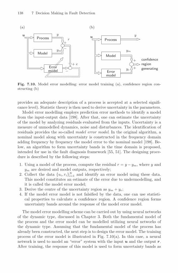
138 7 Decision Making in Fault Detection
(a) (b)
Process
Model
Errormodel
e+
−
r+
−
u y
ym
Process
Model
Errormodel
+
+
u y
ym
ye
confidenceregiongenerating
Fig. 7.10. Model error modelling: error model training (a), confidence region con-structing (b)
provides an adequate description of a process is accepted at a selected signifi-cance level). Statistic theory is then used to derive uncertainty in the parameters.
Model error modelling employs prediction error methods to identify a modelfrom the input-output data [198]. After that, one can estimate the uncertaintyof the model by analyzing residuals evaluated from the inputs. Uncertainty is ameasure of unmodelled dynamics, noise and disturbances. The identification ofresiduals provides the so-called model error model. In the original algorithm, anominal model along with uncertainty is constructed in the frequency domainadding frequency by frequency the model error to the nominal model [198]. Be-low, an algorithm to form uncertainty bands in the time domain is proposed,intended for use in the fault diagnosis framework [55, 51]. The designing proce-dure is described by the following steps:
1. Using a model of the process, compute the residual r = y − ym, where y andym are desired and model outputs, respectively;
2. Collect the data {ui, ri}Ni=1 and identify an error model using these data.
This model constitutes an estimate of the error due to undermodelling, andit is called the model error model;
3. Derive the centre of the uncertainty region as ym + ye;4. If the model error model is not falsified by the data, one can use statisti-
cal properties to calculate a confidence region. A confidence region formsuncertainty bands around the response of the model error model.
The model error modelling scheme can be carried out by using neural networksof the dynamic type, discussed in Chapter 3. Both the fundamental model ofthe process and the error model can be modelled utilizing neural networks ofthe dynamic type. Assuming that the fundamental model of the process hasalready been constructed, the next step is to design the error model. The trainingprocess of the error model is illustrated in Fig. 7.10(a). In this case, a neuralnetwork is used to model an “error” system with the input u and the output r.After training, the response of this model is used to form uncertainty bands as
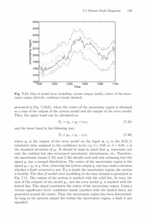
7.3 Robust Fault Diagnosis 139
1000 1020 1040 1060 1080 11001960
1970
1980
1990
2000
2010
2020
2030
2040
2050
Time
Unc
erta
inty
reg
ion
Fig. 7.11. Idea of model error modelling: system output (solid), centre of the uncer-tainty region (dotted), confidence bands (dashed)
presented in Fig. 7.10(b), where the centre of the uncertainy region is obtainedas a sum of the output of the system model and the output of the error model.Then, the upper band can be calculated as
Tu = ym + ye + tβv, (7.45)
and the lower band in the following way:
Tl = ym + ye − tβv, (7.46)
where ye is the output of the error model on the input u, tβ is the N (0, 1)tabulated value assigned to the confidence level, e.g β = 0.05 or β = 0.01, v isthe standard deviation of ye. It should be kept in mind that ye represents notonly the residual but also structured uncertainty, disturbances, etc. Therefore,the uncertainty bands (7.45) and (7.46) should work well only assuming that thesignal ye has a normal distribution. The centre of the uncertainty region is thesignal ym+ye ≈ y. Now, observing the system output y, one may make a decisionwhether a fault occurred or not. If y is inside the uncertainty region, the systemis healthy. The idea of model error modelling in the time domain is presented inFig. 7.11. The output of the system is marked with the solid line. In turn, thesum of the outputs of the model ym and the error model ye is marked with thedotted line. This signal constitutes the centre of the uncertainty region. Using acertain significance level, confidence bands (marked with the dashed lines) aregenerated around the centre. Thus, the uncertainty region has been determined.As long as the process output lies within the uncertainty region, a fault is notsignalled.

140 7 Decision Making in Fault Detection
The key question is to find a proper structure of the error model. As wasdiscussed in [198], one can start with an a priori chosen flexible structure, e.g.the 10-th order FIR filter. If this error model is not falsified by the data, ithas to be kept. Otherwise, the model complexity should be increased until itis unfalsified by the data. In Sections (8.2.4) and (8.3.4), neural network basederror models are discussed.
7.4 Summary
The purpose of this chapter was to introduce methods responsible for makingdecisions about possible faults. It was shown that by using artificial neural net-works an effective residual evaluation can be realized. The first proposed methodof residual evaluation used a simple neural network trained in such a way as tomaximise the output entropy in order to approximate the probability densityfunction of a residual. Thus, a more representative threshold value assigned toa given significance level can be obtained. It was shown that such an approachsignificantly reduces the number of false alarms caused by an inaccurate modelof the process. The proposed density shaping approach can be easily expandedto more complex network topologies in order to estimate more sophisticatedprobability density functions. By using two sigmoidal neurons connected in se-ries it is possible to estimate asymmetric probability density functions and thenumber of false alarms can be even further reduced. It is worth noting that self-organizing training used to adjust the network parameters is very simple andeven tens thousand training steps last a few seconds on a standard PC machine.The second proposed method for residual evaluation was a model error modellingtechnique realized using neural networks intended for use in the time domain.Due to estimating model uncertainty, the robust fault diagnosis system can turnout much more sensitive to the occurrence of small faults than standard decisionmaking methods. Moreover, the number of false alarms can be considerably re-duced. The open problem here is to find a proper model error model. This issueseems to be much more difficult to solve than finding a fundamental model ofthe system.

8 Industrial Applications
This chapter presents the application of artificial neural networks discussed inthe previous chapters to fault diagnosis of industrial processes. Three examplesare considered:
1. fault detection and isolation of selected parts of the sugar evaporator,2. fault detection of selected components of the Fluid Catalytic Crackig (FCC)
process,3. fault detection, isolation and identification of a DC motor.
In all case studies, locally recurrent globally feedforward networks, introducedin Section 3.5.4, are used as models of the industrial processes considered. Othertypes of neural networks, discussed in Sections 7.2 and 7.3.3, are used in decisionmaking in order to detect faults.
The chapter is organized as follows: in Section 8.1, fault detection and isolationof selected parts of the sugar evaporator is presented. In turn, Section 8.2 consistsof results concerning fault detection of selected components of the FCC process.The last example, fault detection, isolation and identification of the DC motor,is shown in Section 8.3.
8.1 Sugar Factory Fault Diagnosis
The problem regarding FDI of the components of the sugar evaporator waswidely considered within the EU DAMADICS project [206, 207]. DAMADICSwas a research project focused on drawing together wide-ranging techniques andfault diagnosis within the framework of a real application to on-line diagnosis ofa 5-stage evaporisation plant of the sugar factory in Lublin, Poland. The sugarfactory was a subcontractor providing real process data and the evaluation oftrials of fault diagnosis methods.
The evaporation station presented below is part of the Lublin Sugar Factory,Poland. In a sugar factory, sucrose juice is extracted by diffusion. This juice isconcentrated in a multiple-stage evaporator to produce a syrup. The liquor goesthrough a series of five stages of vapourisers, and in each passage its sucroseconcentration increases. The sugar evaporation control should be performed in
K. Patan: Artificial. Neural Net. for the Model. & Fault Diagnosis, LNCIS 377, pp. 141–186, 2008.springerlink.com c© Springer-Verlag Berlin Heidelberg 2008

142 8 Industrial Applications
R RR%
%
%
%
t/h
t/h
kPa
kPa
Vapour model
Temperaturemodel
Actuator
m /h3
kPa
Co
Co
Co
Co
CoCoCo
Co
T51 02_
T51 01_
T51 03_ T51 04_
P51 04_
PC51 01_
LC51 03_
LC51 01_TC51 05_
F51 01_
F51 02_
F51 03_
P51 03_
T51 06_
T51 08_
T51 07_
Fig. 8.1. Evaporation station. Four heaters and the first evaporation section
such a way that the energy used is minimised to achieve the required quality ofthe final product. The main inconvenient features that complicate the control ofthe evaporation process are [153, 26]:
• highly complex evaporation structure (large number of interacting compo-nents),
• large time delays and responses (configuration of the evaporator, number ofdelays, capacities),
• strong disturbances caused by violent changes in the steam,• many constrains on several variables.
The filtered and clarified syrup containing ca. 14% of sugar (weak syrup) isdirected to the evaporation station to be condensed, up to about 70% of drysubstance, with minimum heat-energy consumption. The evaporation station iscomposed of five sections of vaporizers. The first three sections are of the Robertstype with a bottom heater-chamber, whereas the last two are of the Wiegendstype with a top heater-chamber. For waste-heat treatment two multi-sectionboilers are used. The heat power supplied to drive the evaporation process isgained from the waste steam of the local power station. This power is used todrive all energy-consuming technological nodes such as preheaters, the evapo-ration station, strike pans and central heating. The saturated vapour generatedduring the evaporation process is fed to the successive sections of vaporizersand to the preheaters. The water condensate from the evaporators is directed tothe waste-heat boilers as well as other devices mentioned above. The waste-heatboilers retrieve heat power by decompressing the condensate in their successivesections. The sugar production process is controlled, monitored and supervisedby the decentralized automatic control system of the Supervisory Control AndData Acquisition (SCADA) type. This system makes it possible to record andstore set-point, control and process variables. These archives can be used totrain neural models off-line. After that, neural models are applied for on-linefault detection and isolation purposes.

8.1 Sugar Factory Fault Diagnosis 143
Table 8.1. Specification of process variables
Variable Description Range
F51 01 Thin juice flow to the input of the evaporation station 0 − 500 m3/h
F51 02 Steam flow to the input of the evaporation station 0 − 100 t/h
P51 03 Vapour pressure in the 1-st section of the evaporator 0 − 250 kPa
T51 06 Input steam temperature 50 − 150 oC
T51 07 Vapour temperature in the 1-st section of the evaporator 50 − 150 oC
T51 08 Juice temperature after the 1-st section of the evaporator 50 − 150 oC
TC51 05 Thin juice temperature after heaters 50 − 150 oC
8.1.1 Instrumentation Faults
Thanks to technological improvement and very careful inspection of the plantbefore starting a 3-month long sugar campaign, faults in sensors, actuators andtechnology are rather exceptional. Therefore, to check on the sensitivity andeffectiveness of the fault detection system designed using dynamic neural net-works, data with artificial faults in measuring circuits are used (the achievedresults are presented in Section 8.1.3). Sensor faults are simulated by increasingor decreasing the values of particular signals by 5, 10 and 20% at specified timeintervals. In Fig. 8.1, the first section of the evaporation station is shown. Inthe figure, most of the accessible measurable variables are marked, and theirspecification is given in Table 8.1. Based on observations of the process variablesand on the knowledge of the process, the following models can be designed andinvestigated [208, 26]:
• Vapour pressure in the vapour chamber of the evaporation section (vapourmodel):
P51 03 = h1(T 51 07); (8.1)
• Juice temperature after the evaporation section (temperature model):
T 51 08 = h2(T 51 06, TC51 05, F51 01, F51 02), (8.2)
where h1(·) and h2(·) are the relations between variables. Suitable process vari-ables are measured by specific sensors at chosen points of the evaporation sta-tion. After that, the obtained data are transferred to the monitoring system andstored there.
8.1.2 Actuator Faults
The actuator to be diagnosed is marked in Fig. 8.1 by the dashed square. Theblock scheme of this device is presented in Fig. 8.2, where measurable processvariables are marked with the dashed lines. The actuator considered consistsof three main parts: the control valve, the linear pneumatic servo-motor andthe positioner [209, 210]. The symbols and process variables are presented in
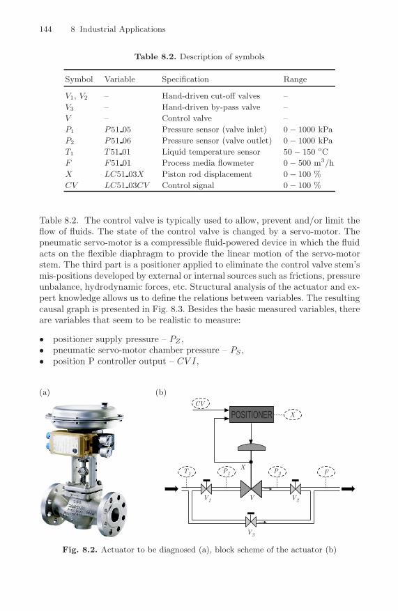
144 8 Industrial Applications
Table 8.2. Description of symbols
Symbol Variable Specification Range
V1, V2 – Hand-driven cut-off valves –
V3 – Hand-driven by-pass valve –
V – Control valve –
P1 P51 05 Pressure sensor (valve inlet) 0 − 1000 kPa
P2 P51 06 Pressure sensor (valve outlet) 0 − 1000 kPa
T1 T51 01 Liquid temperature sensor 50 − 150 oC
F F51 01 Process media flowmeter 0 − 500 m3/h
X LC51 03X Piston rod displacement 0 − 100 %
CV LC51 03CV Control signal 0 − 100 %
Table 8.2. The control valve is typically used to allow, prevent and/or limit theflow of fluids. The state of the control valve is changed by a servo-motor. Thepneumatic servo-motor is a compressible fluid-powered device in which the fluidacts on the flexible diaphragm to provide the linear motion of the servo-motorstem. The third part is a positioner applied to eliminate the control valve stem’smis-positions developed by external or internal sources such as frictions, pressureunbalance, hydrodynamic forces, etc. Structural analysis of the actuator and ex-pert knowledge allows us to define the relations between variables. The resultingcausal graph is presented in Fig. 8.3. Besides the basic measured variables, thereare variables that seem to be realistic to measure:
• positioner supply pressure – PZ ,• pneumatic servo-motor chamber pressure – PS ,• position P controller output – CV I,
(a) (b)
P2 F
X
XP1T1
V1 V2V
V3
CV
POSITIONER
Fig. 8.2. Actuator to be diagnosed (a), block scheme of the actuator (b)

8.1 Sugar Factory Fault Diagnosis 145
and an additional set of unmeasurable physical values useful for structuralanalysis:
• flow through the control valve – FV ,• flow through the by-pass valve – FV 3,• Vena-contacta force – FV C ,• by-pass valve opening ratio – X3.
Taking into account the causal graph presented in Fig. 8.3 and the set of mea-surable variables, the following two relations are considered:
• Servo-motor rod displacement:
X = h3(CV, P1, P2, T1, X); (8.3)
• Flow through the actuator:
F = h4(X, P1, P2, T1), (8.4)
where h3(·) and h4(·) are non-linear functions. Fault isolation is only possible ifdata describing several faulty scenarios are available. Due to safety regulations,it is impossible to generate real faulty data. Therefore, in cooperation with thesugar factory, some faults were simulated by manipulations on process variables.The monitored data acquired from the SCADA system after suitable modifica-tion are introduced back to the controlled system. In this way, one can generateartificial faults that are as realistic as possible. For example, the fully openedby-pass valve scenario causes an increasing flow through the actuator and thesystem responds by throttling the flow in the main pipe. This event can be rec-ognized by observing the CV value. During the experiments, the following faultswere considered [26]:
f1 – positioner supply pressure drop,f2 – unexpected pressure change across the valve,f3 – fully opened by-pass valve.
P1
XCV
P2
PVCVI
T1
FPS
PZ
FV3
FVC X
3
measured variables
variables realistic to measure
unmeasurable variables
Fig. 8.3. Causal graph of the main actuator variables
146 8 Industrial Applications
The first faulty scenario can be caused by many factors such as pressure supplystation faults, oversized system air consumption, air-leading pipe breaks, etc.This is a rapidly developing fault. Physical interpretations of the second faultcan be media pump station failures, increased pipe resistance or external medialeakages. This fault is rapidly developing as well. The last scenario can be causedby valve corrosion or seat sealing wear. This fault is abrupt.
8.1.3 Experiments
Data preprocessing
Individual process variables are characterized by their amplitudes and ranges.In many cases, these signal parameters differ significantly for different processvariables. These large differences may cause the neural model to be trainedinaccurately. Therefore, raw data should be preprocessed. Preprocessing is asequence of operations converting raw data, such as measurements, to a datarepresentation suitable for such processing tasks as modelling, identification orprediction. In this experiment, the inputs of the models under consideration arenormalized according to the formula
xi =
(xi − mi
)vi
, (8.5)
where mi denotes the mean (expected) value of the i-th input, and vi denotes thestandard deviation of the i-th input. The normalization of the inputs guaranteesthat the i-th input has a zero mean and a unit standard deviation. In turn, theoutput data should be transformed taking into consideration the response rangeof the output neurons. For hyperbolic tangent neurons, this range is [−1, 1]. Toperform this transformation, the linear scaling can be adopted:
ys =2(y − a)
b − a− 1, (8.6)
where y and ys are the actual and scaled patterns, respectively, and a and b arethe minimal and maximal values of the process variables, respectively. In orderto achieve the above transformation, the ranges of the suitable process variablesgiven in Tables 8.1 and 8.2 can be used.
Model selection
The purpose of model selection is to identify a model in order to best fit alearning data set. Several information criteria can be used to accomplish thistask [162]. One of them is the Akaike information criterion (4.24), discussed indetail in Section 4.4. Another well-known criterion is the Final Prediction Error(FPE), which selects the model order minimizing the function defined accordingto the formula
fFPE = J1 + K
N
1 − KN
, (8.7)

8.1 Sugar Factory Fault Diagnosis 147
where J is the sum of squared errors between the desired and network outputs,respectively, N is the number of samples used to compute J , and K is the numberof the model parameters. The term (1+K/N)/(1−K/N) decreases with K andrepresents inaccuracies in estimating the model parameters.
Instrumentation fault detection
In order to evaluate the quality of modelling, the performance index is introducedin the form of the sum of squared errors. Testing and training sets are formed thatare inherently based on data from two different working shifts. It is well knownthat model selection should never be performed on the same data that are usedfor the identification of the model itself. Changing the test data, the best modelalso generally changes; however, under a suitable assumption and a set of datarich enough this issue becomes less critical and should not invalidate the proposedapproach. To check on the sensitivity and effectiveness of the proposed faultdetection system, data with artificial faults in measuring circuits are employed.The faults are simulated by increasing or decreasing the values of particularsignals by 5, 10 and 20% at specified time intervals. In the following, experimentalresults on the detection of instrumental faults are reported.
Vapour model
The process to be modelled is described by the formula (8.1). This simple pro-cess has one input and one output. The training process was carried out off-linefor 30000 iterations using the SPSA algorithm of the dynamic network architec-ture (3.39). The parameters of the learning algorithm were as follows: A = 100,a = 0.008, c = 0.01, α = 0.602, and γ = 0.101. The learning set Nu consisted of800 samples whilst the testing set Nt included 3000 samples. The best model wasselected by using the information criteria AIC and FPE. The results of modeldevelopment are presented in Table 8.3, where Nm
r,v,s represents the m-layer dy-namic neural network with r inputs, v hidden neurons and s outputs, K is thenumber of the network parameters, Ju and Jt are the sum of squared errors be-tween the desired and network outputs, calculated for the training and testingsets, respectively. For the training set, the best results (marked with the frames)were obtained for the model of the N2
1,4,1 architecture with the first order filter.However, for the testing set, one can observe that other network structures showbetter performance. In this case, the neural network belongs to the class N2
1,5,1.Each neuron of the dynamic network model is of the first order of the IIR filterand has the hyperbolic tangent activation function. This testifies that this net-work structure has a better generalization ability than the previous one selectedfor the training set. Finally, the model corresponding to the minimum criteriain testing was selected as the optimal one. Figure 8.4 presents the residual sig-nal. Our study includes failures in two sensors: the fault in the measurementP51 03 (time steps 900–1200) and the fault in the measurement T 51 07 (timesteps 1800–2100). In both cases, the faults can be detected immediately andcertainly, e.g. by using a threshold technique according to (7.3) with β = 0.05.In this case, T = 0.05. Taking into account the sensitivity of the proposed faultdetection system, we can state that measuring disturbances smaller than 5% can

148 8 Industrial Applications
Table 8.3. Selection of the neural network for the vapour model
Network Filter Training Testing
structure order K Ju fFPE fAIC Jt fFPE fAIC
N21,2,1 2 28 0,1080 0,1158 -0,8966 0,639 0,6510 -0,1758
N21,3,1 2 38 0,0946 0,1040 -0,9291 0,674 0,6913 -0,1460
N21,4,1 1 35 0,0745 0,0813 -1,0403 0,622 0,6366 -0,1828
N21,5,1 1 46 0,0832 0,0934 -0,9649 0,607 0,6259 -0,1861
N21,5,1 1 46 0,0763 0,0856 -1,0025 0,703 0,7249 -0,1224
N21,5,1 2 58 0,1180 0,1364 -0,7831 0,992 1,0311 0,0352
be easily detected. Unfortunately, in Fig. 8.4 we can see that the fault detectionsystem generates a certain number of false alarms. Some of them, like that at thetime step 1750, can be caused by disturbances or noise; however, there is alsoa false alarm (at about the time step 200), which was caused by an inaccuratemodel. One of the possible solutions is to use a more accurate model of the sys-tem considered. If it is impossible to find a better model, an adaptive thresholdtechnique may be applied, which is much more robust than the fixed threshold.
Temperature model
The process to be modelled is described by the formula (8.2). This process hasone output and four inputs. The training process was carried out off-line for30000 iterations using the SPSA algorithm of the dynamic network architecture.
Fig. 8.4. Residual signal for the vapour model in different faulty situations: fault inP51 03 (900–1200), fault in T51 07 (1800–2100)

8.1 Sugar Factory Fault Diagnosis 149
Fig. 8.5. Residual signals for the temperature model in different faulty situations:fault in F51 01 (0–300), fault in F51 02 (325–605), fault in T51 06 (1500-1800), faultin T51 08 (2100–2400), fault in TC51 05 (2450–2750)
The parameters of the learning algorithm were as follows: A = 1000, a = 0.04,c = 0.01, α = 0.602, and γ = 0.101. The learning set consisted of 800 samples.For the training set, the best results were obtained for the model of the N2
4,4,1architecture with the first order filter. However, for the testing set, one can ob-serve that other network structures show better performance. In this case, theneural network belongs to the class N2
4,3,1. Each neuron of the dynamic networkmodel is of the first order of the IIR filter and has the hyperbolic tangent activa-tion function. Figure 8.5 presents the residuals for simulated failures of differentsensors. The following sensor faults were successively introduced at chosen timeintervals: the fault in the measurement F51 01 (time steps 0–300), the faultin the measurement F51 02 (time steps 325–605), the fault in the measurementT 51 06 (time steps 1500-1800), the fault in the output sensor T 51 08 (time steps2100–2400) and the fault in the measurement TC51 05 (time steps 2450–2750).In this study, the threshold applied was equal to 0.04. As can be seen in Fig. 8.5,the fault detection system is most sensitive to the failures of the output sensor– T 51 08 (time steps 2100–2400). Even sensor failures smaller than 5% can beimmediately detected. Somewhat worse are diagnosis results for the faults of thesensors T 51 06 (time steps 1500-1800) and TC51 05 (time steps 2450–2750). Inboth cases, 5% of the failures are explicitly and surely detected by the proposedfault detection system. For the sensor TC51 05, however, one can observe thatonly -5, -10 and -20% faults are distinctly and surely detected. +5, +10 and+20% faults are signalled by small spikes only, whose occurrence in the resid-uals is due to noise effects rather than fault occurrences. The worst results are

150 8 Industrial Applications
obtained for the failures of the sensors F51 01 (time steps 0–300) and F51 02(time steps 325–605). Only large faults in both sensors are shown by the resid-uals. This means that the fault detection system is not very sensitive to theoccurrence of faults in these two sensors.
Robust instrumentation fault detection
Adaptation of the threshold
Analyzing the residual signal in the fault-free case, one can see that in some timeintervals there are large deviations of the residuals from zero. Unfortunately,these deviations, caused by disturbances or modelling errors, can generate falsealarms during residual evaluation. In order to avoid false alarms, it is necessaryto analyze how changes of inputs and outputs of the process influence deviationsof the residual from zero. Such knowledge can be elaborated in the form ofthe adaptive threshold (7.43) by means of fuzzy rules. Two sample fuzzy rules,which take into account the modelling mismatch of the vapour model, are givenbelow [54]:
R1: If {u is zero} and {yp is zero} then {ΔJ is large};
R2: If {u is small positive} and {yp is zero} then {ΔJ is medium}.
The linguistic variables zero, large, small positive and medium are defined bythe relevant membership functions. To realize such a kind of threshold, the FuzzyLogic Toolbox for Matlab 5.3 was used. The number of linguistic variables, aswell as the shape of membership functions, is chosen experimentally. The defuzzi-fication process is carried out using the centre of area method. A comparisonof the constant and adaptive thresholds, in the case of the temperature model,is shown in Fig. 8.6. The value of the constant threshold shown in Fig. 8.6(a)is set as a sum of the mean value and the standard deviation of the residualaccording to (7.5) with ζ = 1. In this case, the number of false alarms is quitehigh. It is easy to see that the false alarms which occurred in the case of theconstant threshold can be avoided with a suitably adjusted adaptive threshold(Fig. 8.6(b)). In the case of the adaptive threshold, the number of false alarmswas reduced even three times. Table 8.4 contains the number of false alarmsgenerated using both the constant and adaptive thresholds, for all investigatedmodels. In all cases the number of false alarms is reduced considerably.
Table 8.4. Number of false alarms
Model Number of false alarms
constant threshold adaptive threshold
temperature model 399 132
vapour model 226 76
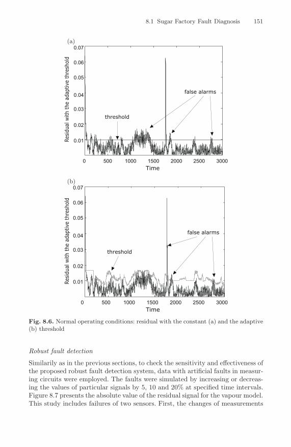
8.1 Sugar Factory Fault Diagnosis 151
(a)
0.01
0.02
0.03
0.04
0.05
0.06
0.07
0 500 1000
Resi
dualw
ith
the
adaptive
thre
shold
1500 2000 2500 3000
false alarms
threshold
Time
(b)
0.01
0.02
0.03
0.04
0.05
0.06
0.07
0 500 1000
Resi
dualw
ith
the
adaptive
thre
shold
1500 2000 2500 3000
false alarms
threshold
Time
Fig. 8.6. Normal operating conditions: residual with the constant (a) and the adaptive(b) threshold
Robust fault detection
Similarily as in the previous sections, to check the sensitivity and effectiveness ofthe proposed robust fault detection system, data with artificial faults in measur-ing circuits were employed. The faults were simulated by increasing or decreas-ing the values of particular signals by 5, 10 and 20% at specified time intervals.Figure 8.7 presents the absolute value of the residual signal for the vapour model.This study includes failures of two sensors. First, the changes of measurements

152 8 Industrial Applications
in turn by +5%, +10%, +20%, -5%, -10% and -20% in the sensor P51 03 wereintroduced (at the time steps 900–1200). After that, similar failures in the sensorF51 04 were studied (at the time steps 1800–2100). In both cases, the faults aredetected immediately and surely. Taking into account the sensitivity of the pro-posed fault detection system it can be stated that even sensor failures smallerthan 5% can be detected easily. Moreover, using the adaptive threshold tech-nique, the fault detection system can avoid a certain number of false alarms.Taking into account these experimental results, one can conclude that the pro-posed robust fault detections system is very sensitive to the occurrence of faults.Using the adaptive threshold technique, it is possible to considerably reduce thenumber of false alarms caused by modelling errors. However, problems of theselection of fuzzy model components such as the number of linguistic variables,the shape of membership functions or the generation of rules are still open.
Fig. 8.7. Residual for different faulty situations
Actuator fault detection and isolation
In the proposed FDI system, four classes of the system behaviour – the normaloperating condition f0 and three faults: f1–f3 – are modelled by a bank ofdynamic neural networks, according to the scheme presented in Fig. 2.4. Toidentify the models (8.3) and (8.4), dynamic neural networks with four inputsand two outputs were applied:[
X
F
]= NN(P1, P2, T1, CV ), (8.8)
where NN is the neural model. Multi-Input Multi-Output (MIMO) models areconsidered taking into account two reasons. The first one is the computational

8.1 Sugar Factory Fault Diagnosis 153
Table 8.5. Neural models for nominal conditions and faulty scenarios
Faulty scenario Structure Filter order Activation function
f0 N24,5,2 2 hyperbolic tangent
f1 N24,7,2 1 hyperbolic tangent
f2 N24,7,2 1 hyperbolic tangent
f3 N24,5,2 1 hyperbolic tangent
effort during identification. Each neural model considered can be representedby the two Multi-Input Single-Output (MISO) models, for which the trainingprocess can be easier to perform. Unfortunately, in the case when some numberof faults are considered, let us say 10, it is required to design 20 MISO modelsinstead of 10 of the MIMO type. The training and testing sets are differentand formed similarly as in the case of instrumentation fault detection (see theprevious paragraphs). All models were trained and selected as in the previoustwo examples, but details concerning the proper model selection are not givenhere. The final neural model specification is presented in Table 8.5. The selectedneural networks have a relatively small structure. Only two processing layers with5 or 7 hidden elements are enough to identify faults with pretty high accuracy.Moreover, dynamic neurons have hyberbolic tangent activation functions andfirst order IIR filters. Each neural model was trained using suitable faulty data.Subsequently, the performances of the constructed models were examined usingboth nominal and faulty data. Both fault detection and isolation are performedusing the thresholding described by (7.3) assuming the significance level β = 0.05(5%). The experimental results are reported in the forthcoming sections.
Fault detection
Fault detection is performed using the model representing nominal operatingconditions. The threshold corresponding to the output F was found as Tf =0.0256, and the threshold for the output X as Tx = 0.0322. The residuals for thismodel should not be greater than the thresholds when the actuator is healthy,and should exceed the thresholds in faulty cases. Figures 8.8 and 8.9 show thebehaviour of both nominal model residuals in various faulty scenarios. For clarityof presentation, thresholds levels are not presented there. The thick line repre-sents the time instant when a fault occurred. It is clearly shown that all thefaults are reliable and surely detected. At this stage, of course, it is impossibleto find out what exactly happen. In order to localize a fault it is necessary toperform fault isolation.
Fault isolation
Fault f1. The first fault was simulated at the time step 270 and lasted about 275time steps. In order to isolate this fault, the residuals generated by the fault modelf1 should be near zero, other fault models should generate residuals different thanzero. Figure 8.10 shows the residuals for all fault models. One can observe that this

154 8 Industrial Applications
(a)
(b)
(c)
Fig. 8.8. Residual of the nominal model (output F ) in the case of the faults f1 (a),f2 (b) and f3 (c)
fault is isolated because only the residual in Fig. 8.10(a) is near zero during theoccurrence of f1. Simultaneously, the residual in Fig. 8.10(a) is near zero undernominal operating conditions (and it should be different than zero). This meansthat the related model generates a large number of false alarms.
Fault f2. The next faulty scenario was simulated at the time step 775 (pressureoff) till the time step 1395 (pressure on). Figure 8.11 presents the residuals ofthe fault models for this case. Using the residuals obtained from the output F ofthe models one can conclude that this fault is not isolable, because two residuals(Figs. 8.11(b) and 8.11(c)) tend to zero. Fortunately, there is a chance to isolatethis fault using the output X of the models. Only the fault model f2 generatesa residual near zero (Fig.8.11(e)). In this case, however, the residual is stronglyoscilating, which can result in quite a large number of false alarms.
Fault f3. The third fault was simulated at the time step 860 (valve opening)till the time step 1860 (valve closing). In this case, the fault is reliably isolated

8.1 Sugar Factory Fault Diagnosis 155
(a)
(b)
(c)
Fig. 8.9. Residual of the nominal model (output X) in the case of the faults f1 (a),f2 (b) and f3 (c)
using the outputs X of the neural models. Only one residual (Fig. 8.12(f)) isnear zero when the fault occurs. Similarly as in the previous study, the faultis not isolable using the outputs F of the models. Two of the residuals tendto zero: the residual for the fault f1 (Fig.8.12(a)) and the one for the fault f3(Fig. 8.12(c)).
Decision making is performed using the thresholding technique described by(7.3) with β = 0.05. The threshold values can be found in the paragraph onFault detection for the nominal model and in Table 8.8 for fault models. Theresults of fault detection are presented in Table 8.6(a). One can see there that allfaults are detected by the proposed system either using the nominal model of theflow F or the nominal model of the rod displacement X . In turn, fault isolationresults are shown in Table 8.6(b). The main result here is the fact that the faultf1 cannot be isolated by neural models. The second result shows that the faultsf2 and f3 can be isolated using only fault models of the rod displacement. Faultmodels of the flow cannot locate a fault which occurred in the system.

156 8 Industrial Applications
(a)
(b)
(c)
(d)
(e)
(f)
Fig. 8.10. Residuals of the fault models f1 (a) and (d); f2 (b) and (e); f3 (c) and (f)in the case of the fault f1

8.1 Sugar Factory Fault Diagnosis 157
(a)
(b)
(c)
(d)
(e)
(f)
Fig. 8.11. Residuals of the fault models f1 (a) and (d); f2 (b) and (e); f3 (c) and (f)in the case of the fault f2

158 8 Industrial Applications
(a)
(b)
(c)
(d)
(e)
(f)
Fig. 8.12. Residuals of the fault models f1 (a) and (d); f2 (b) and (e); f3 (c) and (f)in the case of the fault f3

8.1 Sugar Factory Fault Diagnosis 159
Table 8.6. Results of fault detection (a) and isolation (b) (X – detectable/isolable, N– not detectable/not isolable)
(a) (b)
Fault detection results
Faulty scenario f1 f2 f3
flow model X X X
rod displacement model X X X
Fault isolation results
Faulty scenario f1 f2 f3
flow model N N N
rod displacement model N X X
Qualitative analysis of the fault detection and isolation system consideredis presented in the next section, together with a comparison with alternativeapproaches.
Comparative study
To check the efficiency of the proposed fault detection and isolation system, theLocally Recurrent (LR) network trained with SPSA is compared with alterna-tive approaches such as Auto-Regressive with eXogenous inputs (ARX) models[162] and Neural Networks Auto-Regressive with eXogenous inputs (NNARX)models [19]. The simulations are performed over the processes (8.3) and (8.4).All structures of the models used are selected experimentally. To compare theachieved results, the following performance indices are used:
• modelling quality in the form of a sum of squared errors between the desiredand the actual response of the model calculated using a testing set,
• detection time,• false detection rate (2.25),• isolation time,• false isolation rate (2.27).
The first comparative study shows the modelling quality of the modelsachieved by using the examined methods. The modelling quality represents pre-diction capabilities of the models and is calculated as a sum of squared errorsover the testing set. The achieved results are shown in Table 8.7. As one can see,the worst result was obtained for the ARX models. The actuator is described by
Table 8.7. Modelling quality for different models
Method f0 f1 f2 f3
F X F X F X F X
LR 0.73 0.46 0.02 0.91 0.098 0.139 2.32 12.27
ARX 2.52 5.38 4.93 14.39 11.92 16.96 19.9 4.91
NNARX 0.43 0.71 0.089 0.1551 0.6 2, 17 0.277 22.5
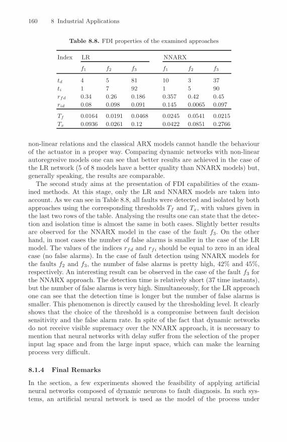
160 8 Industrial Applications
Table 8.8. FDI properties of the examined approaches
Index LR NNARX
f1 f2 f3 f1 f2 f3
td 4 5 81 10 3 37
ti 1 7 92 1 5 90
rfd 0.34 0.26 0.186 0.357 0.42 0.45
rid 0.08 0.098 0.091 0.145 0.0065 0.097
Tf 0.0164 0.0191 0.0468 0.0245 0.0541 0.0215
Tx 0.0936 0.0261 0.12 0.0422 0.0851 0.2766
non-linear relations and the classical ARX models cannot handle the behaviourof the actuator in a proper way. Comparing dynamic networks with non-linearautoregresive models one can see that better results are achieved in the case ofthe LR network (5 of 8 models have a better quality than NNARX models) but,generally speaking, the results are comparable.
The second study aims at the presentation of FDI capabilities of the exam-ined methods. At this stage, only the LR and NNARX models are taken intoaccount. As we can see in Table 8.8, all faults were detected and isolated by bothapproaches using the corresponding thresholds Tf and Tx, with values given inthe last two rows of the table. Analysing the results one can state that the detec-tion and isolation time is almost the same in both cases. Slightly better resultsare observed for the NNARX model in the case of the fault f3. On the otherhand, in most cases the number of false alarms is smaller in the case of the LRmodel. The values of the indices rfd and rfi should be equal to zero in an idealcase (no false alarms). In the case of fault detection using NNARX models forthe faults f2 and f3, the number of false alarms is pretty high, 42% and 45%,respectively. An interesting result can be observed in the case of the fault f3 forthe NNARX approach. The detection time is relatively short (37 time instants),but the number of false alarms is very high. Simultaneously, for the LR approachone can see that the detection time is longer but the number of false alarms issmaller. This phenomenon is directly caused by the thresholding level. It clearlyshows that the choice of the threshold is a compromise between fault decisionsensitivity and the false alarm rate. In spite of the fact that dynamic networksdo not receive visible supremacy over the NNARX approach, it is necessary tomention that neural networks with delay suffer from the selection of the properinput lag space and from the large input space, which can make the learningprocess very difficult.
8.1.4 Final Remarks
In the section, a few experiments showed the feasibility of applying artificialneural networks composed of dynamic neurons to fault diagnosis. In such sys-tems, an artificial neural network is used as the model of the process under
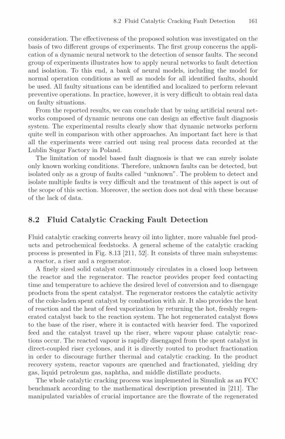
8.2 Fluid Catalytic Cracking Fault Detection 161
consideration. The effectiveness of the proposed solution was investigated on thebasis of two different groups of experiments. The first group concerns the appli-cation of a dynamic neural network to the detection of sensor faults. The secondgroup of experiments illustrates how to apply neural networks to fault detectionand isolation. To this end, a bank of neural models, including the model fornormal operation conditions as well as models for all identified faults, shouldbe used. All faulty situations can be identified and localized to perform relevantpreventive operations. In practice, however, it is very difficult to obtain real dataon faulty situations.
From the reported results, we can conclude that by using artificial neural net-works composed of dynamic neurons one can design an effective fault diagnosissystem. The experimental results clearly show that dynamic networks performquite well in comparison with other approaches. An important fact here is thatall the experiments were carried out using real process data recorded at theLublin Sugar Factory in Poland.
The limitation of model based fault diagnosis is that we can surely isolateonly known working conditions. Therefore, unknown faults can be detected, butisolated only as a group of faults called “unknown”. The problem to detect andisolate multiple faults is very difficult and the treatment of this aspect is out ofthe scope of this section. Moreover, the section does not deal with these becauseof the lack of data.
8.2 Fluid Catalytic Cracking Fault Detection
Fluid catalytic cracking converts heavy oil into lighter, more valuable fuel prod-ucts and petrochemical feedstocks. A general scheme of the catalytic crackingprocess is presented in Fig. 8.13 [211, 52]. It consists of three main subsystems:a reactor, a riser and a regenerator.
A finely sized solid catalyst continuously circulates in a closed loop betweenthe reactor and the regenerator. The reactor provides proper feed contactingtime and temperature to achieve the desired level of conversion and to disengageproducts from the spent catalyst. The regenerator restores the catalytic activityof the coke-laden spent catalyst by combustion with air. It also provides the heatof reaction and the heat of feed vaporization by returning the hot, freshly regen-erated catalyst back to the reaction system. The hot regenerated catalyst flowsto the base of the riser, where it is contacted with heavier feed. The vaporizedfeed and the catalyst travel up the riser, where vapour phase catalytic reac-tions occur. The reacted vapour is rapidly disengaged from the spent catalyst indirect-coupled riser cyclones, and it is directly routed to product fractionationin order to discourage further thermal and catalytic cracking. In the productrecovery system, reactor vapours are quenched and fractionated, yielding drygas, liquid petroleum gas, naphtha, and middle distillate products.
The whole catalytic cracking process was implemented in Simulink as an FCCbenchmark according to the mathematical description presented in [211]. Themanipulated variables of crucial importance are the flowrate of the regenerated

162 8 Industrial Applications
regene-rator
reactorvessel
feed
air
gas
products
riser
Rar
Tfp
Trg1 Trg2
Td1
Trx
Tdg
Fig. 8.13. General scheme of the fluid catalytic cracking converter
catalyst to the riser and the flowrate of combustion air to the regenerator beds.The available measurement variables are presented in Table 8.9. Taking intoaccount expert knowledge about the technological process, one can design thefollowing relations between variables:
• Temperature of the cracking mixture:
Trx = h1(Trg2, Tfp, Trx); (8.9)
• Temperature of the dense phase at the regenerator first stage:
Trg1 = h2(Trg1, Tar, Rar); (8.10)
• Temperature of the dense phase at the regenerator second stage:
Trg2 = h3(Trg1, Tar, Rar); (8.11)
• Temperature of the regenerator first stage dilute phase:
Td1 = h4(Trg1); (8.12)
• Temperature of the general dilute phase:
Tdg = h5(Td1). (8.13)
In order to design a fault diagnosis system for the FCC process, a model basedscheme is applied. The residual generation block is realized using locally recur-rent networks, described in detail in Section 3.5.4. In turn, residual evaluationis carried out by using statistical analysis, discussed in Section 7.2.2, and MEM,presented in Section 7.3.3. The complete fault diagnosis system is evaluatedusing several faulty scenarios.

8.2 Fluid Catalytic Cracking Fault Detection 163
Table 8.9. Specification of measurable process variables
Variable Description
Rar air flowrate to the regenerator [ton/h]
Tar air temperature [oC]
Tfp feed temperature at the riser entrance [oC]
Trx temperature of the cracking mixture in the riser [oC]
Trg1 temperature of the dense phase at the regenerator first stage [oC]
Trg2 temperature of the dense phase at the regenerator second stage [oC]
Td1 temperature of the regenerator first stage dilute phase [oC]
Tdg temperature of the general dilute phase [oC]
8.2.1 Process Modelling
A locally recurrent neural network is used to describe the process under normaloperating conditions. First, the network has to be trained for this task. Thetraining data were collected from the FCC benchmark. The network was trainedusing the ARS algorithm to mimic the behaviour of the temperature of thecracking mixture (8.9). The neural model (3.39) has three inputs, Trg2(k), Tfp(k)and Trx(k), one output, Trx(k + 1), and consists of three hidden neurons, withthe hyperbolic tangent activation function and the second order IIR filter each.The structure of the network was selected using the ”trial and error” procedure.The model with the smallest value of the criterion in the form of a sum of squarederrors calculated using the testing set is selected as the best one. The trainingwas carried out off-line for 50 steps using 1000 samples. The sum of squarederrors calculated over 7000 testing samples is equal to 169.31. The modelling
10 20 30 40 50 60 70 80 90 100−0.5
0
0.5
1
1.5
2
Time
Sys
tem
and
mod
el o
utpu
ts
Fig. 8.14. Results of modelling the temperature of the cracking mixture (8.9)

164 8 Industrial Applications
0 1000 2000 3000 4000 5000 6000 7000−1.5
−1
−0.5
0
0.5
1
Time
Res
idua
l
Fig. 8.15. Residual signal
results for 100 testing samples are shown in Fig. 8.14, where the model outputis marked by the dotted line and the output of the process by the solid line. Inturn, the residual signal is presented in Fig. 8.15. Although the model mimicsthe behaviour of the process quite well, at some time instances there are largedifferences between the process and model outputs.
8.2.2 Faulty Scenarios
The FCC benchmark makes it possible to simulate a number of faulty scenarios.During the experiments the following scenarios were examined [212, 213, 46]:
1. scenario f1 – 10 % increase in catalyst density,2. scenario f2 – 15% decrease in the weir constant of the first and second stages,3. scenario f3 – 10% decrease in the CO2/CO ratio constant.
These faulty scenarios were implemented in Simulink/Matlab as an additionalcomponent of the mentioned FCC benchmark.
8.2.3 Fault Diagnosis
Normality testing
The comparison between the cumulative distribution function of the normaldistribution F (x) (solid line) and the residual one Fr(x) (dotted line) is presentedin Fig. 8.16. As one can observe, the normality assumption does not seem notto be valid in this case. The cumulative distribution function of the residualshows that its probability density function is a little bit asymmetric. In turn,the probability plot for the residual is presented in Fig. 8.17. This plot clearly
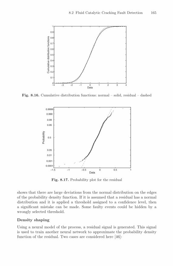
8.2 Fluid Catalytic Cracking Fault Detection 165
−4 −3 −2 −1 0 1 2 3 40
0.1
0.2
0.3
0.4
0.5
0.6
0.7
0.8
0.9
1
Data
Cum
ulat
ive
dist
ribut
ion
func
tions
Fig. 8.16. Cumulative distribution functions: normal – solid, residual – dashed
−1.5 −1 −0.5 0 0.5 1
0.0001
0.001
0.01
0.05
0.5
0.95
0.99
0.999
0.9999
Data
Pro
babi
lity
Fig. 8.17. Probability plot for the residual
shows that there are large deviations from the normal distribution on the edgesof the probability density function. If it is assumed that a residual has a normaldistribution and it is applied a threshold assigned to a confidence level, thena significant mistake can be made. Some faulty events could be hidden by awrongly selected threshold.
Density shaping
Using a neural model of the process, a residual signal is generated. This signalis used to train another neural network to approximate the probability densityfunction of the residual. Two cases are considered here [46]:

166 8 Industrial Applications
Case 1. Estimate of the residual propability density function (7.20)In this case, the neural network (7.17) is trained on-line for 90000 steps using un-supervised learning (update rules (7.18) and (7.19)), described in Section 7.22.2.The final network parameters are w = −14.539 and b = −1.297. The resid-ual histogram and the estimated probability density function are presented inFig. 8.18(a) and (b), respectively. In this case, the estimated distribution functionis symmetric with cut-off values determined for the significance level β = 0.05 arexl = −0.34 and xr = 0.163, and the threshold is equal to T = 0.354 (Fig. 8.18(c)).
Case 2. Estimate of the residual probability density function (7.28)In this case, the neural network (7.21) is trained on-line for 90000 steps usingunsupervised learning (update rules (7.24)–(7.27)), described in Section 7.2.2.The final network parameters are w1 = −5.27, w2 = −11.475, b1 = −0.481and b2 = 5.626. The residual histogram and the estimated probability densityfunction are presented in Fig. 8.19(a) and (b), respectively. In this case, theestimated distribution function has a wider shape than in the previous caseconsidered (Fig. 8.19(c)). The cut-off values determined for the significance levelβ = 0.05 are xl = −0.358 and xr = 0.19 with the threshold T = 0.25.
(a) (b)
−1 −0.8 −0.6 −0.4 −0.2 0 0.2 0.4 0.60
200
400
600
800
1000
1200
1400
1600
1800
2000
Data0 0.2 0.4 0.6 0.8 1
0
50
100
150
200
250
300
350
400
450
Data
(c)
−1 −0.8 −0.6 −0.4 −0.2 0 0.2 0.4 0.60
0.5
1
1.5
2
2.5
3
3.5
4
Data xrxl
Fig. 8.18. Residual histogram (a), network output histogram (b), estimated PDF andthe confidence interval (c)

8.2 Fluid Catalytic Cracking Fault Detection 167
(a) (b)
−1 −0.8 −0.6 −0.4 −0.2 0 0.2 0.4 0.60
200
400
600
800
1000
1200
1400
1600
1800
2000
Data0 0.2 0.4 0.6 0.8 1
0
50
100
150
200
250
300
350
400
450
500
Data
(c)
−1 −0.8 −0.6 −0.4 −0.2 0 0.2 0.4 0.60
0.5
1
1.5
2
2.5
3
3.5
4
Data xrxl
Fig. 8.19. Residual histogram (a), network output histogram (b), estimated PDF andthe confidence interval (c)
Sensitivity
To perform a decision, a significance level β = 0.05 is assumed. The sensitivityof the proposed fault diagnosis system in the fault-free case is checked using theso-called false detection rate (2.25). If it is assumed that the residual has thenormal disribution, the upper threshold is equal to Tu = 0.1068, the lower one toTl = −0.2975 and rfd = 0.0732. The proposed density shaping using the singleneuron (7.17) gives the threshold T = 0.354 and rfd = 0.034, which is a numberof false alarms more than two times smaller than in the case of the normalityassumption. Even better results are obtained for density shaping using the morecomplex neural network (7.21). In this case, the threshold T = 0.25 and thefalse detection rate rfd = 0.0259. The generalization ability of both networks ispretty good, because by assuming the significance level β = 0.05 statistically 5%of samples are allowed to pass the threshold. The achieved result for the network(7.17) is 3.4%, and for the network (7.21) it is 2.59%.
The next experiment shows the relationship between the significance levelassumed and false detection ratios for application for respectively, normal dis-tribution statistics and density shaping using a single neuron. The results are

168 8 Industrial Applications
Table 8.10. Comparison of false detection rates
β rNfd rD
fd Ratio rNfd/rD
fd
0.05 0.0732 0.034 2.153
0.01 0.022 0.0083 2.65
0.001 0.007 0.0011 6.36
presented in Table 8.10, where rNfd is the false detection rate calculated assum-
ing the normal distribution of a residual, and rDfd is the false detection rate of
the density shaping method. These results clearly indicate the advantages of thedensity shaping method. As one can observe, for smaller values of significancelevels the disproportion between false detection rates represented by the ratiorNfd/rD
fd increases. This result confirms the analysis undertaken based on theprobability plot (Fig. 8.17). If normal distribution statistics are used for deci-sion making, then significant mistakes are made, especially using small values ofthe significance level, e.g. β = 0.001.
Fault detection
The results of fault detection are presented in Table 8.11. In each case the truedetection rate (2.26) is close to one, which means that the detection of faults isperformed surely. In order to perform a decision about faults and to determinethe detection time tdt, a time window with the length n = 10 was used. Ifduring the following n time steps the residual exceeds the threshold, then a faultis signalled. The application of the time window prevents the situation whentemporary true detection signals a fault (see Fig. 2.11).
Detection time indices are shown in the last column of Table 8.11. The faultf2 is detected relatively fast. More time is needed to detect the faults f1 andf3. All faulty scenarios can be classified as abrupt faults. It is observed that thefault f3 is developing slower than the faults f1 and f2, so the fault diagnosissystem needs more time to make a proper decision.
Table 8.11. Performance indices for faulty scenarios
Faulty scenario start-up time fault time horizon rtd tdt
f1 7890 9000 0.9315 90
f2 7890 9000 0.9883 14
f3 7890 9000 0.8685 151
8.2.4 Robust Fault Diagnosis
Confidence Bands
In this experiment, decision making is carried out using uncertainty boundsobtained by using model error modelling, discussed in Section 7.3.3. The error

8.2 Fluid Catalytic Cracking Fault Detection 169
model was designed using the NNARX type neural network [55]. Many neuralarchitectures have been examined by the “trial and error” method. The bestperforming two-layer network consists of four hidden neurons with hyperbolictangent activation functions and one linear output element. The number of theinput delays na and the output delays nb is equal to 5 and 15, respectively. Theconclusion is that to capture residual dynamics, a high order model is required.The output of the error model along with the residual is shown in Fig. 8.20.
To determine confidence bands, the 95% significance level was assumed (β =0.05). The uncertainty region (dashed lines) along with the output of the healthysystem (solid line) is shown in Fig. 8.21. The false detection rate in this case isrfd = 0.0472. In the cases when there are rapid changes of the output signal witha large amplitude, the uncertainty region is relatively narrow. This situation isdepicted in Fig. 8.21 at the 40-th time step, when the output signal exceedsthe uncertainty region. For comparison, let us analyze the simple thresholdingcalculated using (7.3), depicted in Fig. 8.22. The false detection rate in this caseis rfd = 0.0734. This is a result more than 1.5 times worse in relation to theadaptive technique based on MEM.
7300 7350 7400 7450 7500−0.2
−0.1
0
0.1
0.2
0.3
0.4
0.5
0.6
Time
Res
idua
l and
mod
el e
rror
out
put
Fig. 8.20. Residual (solid) and the error model output (dashed) under nominal oper-ating conditions
Table 8.12. Performance indices for faulty scenarios
Faulty scenario start-up time fault time horizon rtd tdt
f1 7890 9000 0.9613 40
f2 7890 9000 0.9919 24
f3 7890 9000 0.9207 80

170 8 Industrial Applications
0 10 20 30 40 50
−1.2
−1
−0.8
−0.6
−0.4
−0.2
0
0.2
0.4
0.6
Time
Sys
tem
out
put a
nd c
onfid
ence
ban
ds
Fig. 8.21. Confidence bands and the system output under nominal operatingconditions
0 200 400 600 800 1000−0.8
−0.6
−0.4
−0.2
0
0.2
0.4
Time
Res
idua
l and
thre
shol
ds
Fig. 8.22. Residual with constant thresholds under nominal operating conditions
Fault Detection
The results of fault detection are presented in Fig. 8.23 and Table 8.12. InFig. 8.23, the uncertainty bands are marked by the dashed lines and the systemoutput with the solid one. The achieved results confirm that the robust techniquefor fault diagnosis based on MEM is more sensitive to the occurrence of faultsthan decision making algorithms based on constant thresholds (compare the true

8.2 Fluid Catalytic Cracking Fault Detection 171
(a)
7880 7890 7900 7910 7920 7930 7940 7950−1
−0.5
0
0.5
1
1.5
Time
Con
fiden
ce b
ands
faulthealthy
(b)
7880 7885 7890 7895 7900 7905 7910 7915−1
−0.5
0
0.5
1
1.5
2
2.5
3
3.5
Time
Con
fiden
ce b
ands
faulthealthy
(c)
7870 7880 7890 7900 7910 7920 7930 7940 7950 7960 7970−1
−0.5
0
0.5
1
1.5
Time
Con
fiden
ce b
ands
faulthealthy
Fig. 8.23. Fault detection results: scenario f1 (a), scenario f2 (b), scenario f3 (c)

172 8 Industrial Applications
detection rates in Tables 8.11 and 8.12). For the faults f1 and f3, the detectiontime is also shorter. Solely in the case of the scenario f2, MEM required moretime to make a proper decision, in spite of the fact that this fault was relativelymore quickly detected than the other two.
8.2.5 Final Remarks
In the section it was shown that by using artificial neural networks a model basedfault detection system for chosen parts of the FCC technological process can bedesigned. The experiments show that the locally recurrent network can modela complex technological process with pretty good accuracy. In turn, a simpleneural network trained to maximise the output entropy can approximate theprobability density function of a residual and in this way a more representativethreshold value can be obtained with a given significance level. It was shown thatsuch an approach significantly reduces the number of false alarms caused by aninaccurate model of the process. The proposed density shaping approach can beeasily expanded to more complex network topologies in order to estimate moresophisticated probability distribution functions. By using two sigmoidal neuronsconnected in series it is possible to estimate asymmetric probability densityfunctions and the number of false alarms can be even further reduced. It is worthnoting that self-organizing training used to adjust the network parameters is verysimple and even tens thousand training steps last a few seconds on a standard PCmachine. Better fault detection results were obtained for a robust fault detectionsystem based on neural network realization of model error modelling. In theframework of MEM, the locally recurrent network was used to model the processunder normal operating conditions and then the NNARX model was used toidentify the error model (residual). The experiments show that the proposedmethod gives promising results. An open problem here is to find a proper errormodel. This problem seems to be much more difficult to solve than finding afundamental model of the system.
8.3 DC Motor Fault Diagnosis
Electrical motors play a very important role in safe and efficient work of modernindustrial plants and processes [214]. Early diagnosis of abnormal and faultystates renders it possible to perform important preventing actions, and it al-lows one to avoid heavy economic losses involved in stopped production, thereplacement of elements or parts [10]. To keep an electrical machine in the bestcondition, several techniques such as fault monitoring or diagnosis should beimplemented. Conventional DC motors are very popular, because they are rea-sonably cheap and easy to control. Unfortunately, their main drawback is themechanical collector, which has only a limited life spam. In addition, brush spark-ing can destroy the rotor coil, generate electromagnetic compatibility problemsand reduce insulation resistance to an unacceptable limit [215]. Moreover, inmany cases, electrical motors operate in closed-loop control and small faults of-ten remain hidden by the control loop. It is only if the whole device fails that

8.3 DC Motor Fault Diagnosis 173
the failure becomes visible. Therefore, there is a need to detect and isolate faultsas early as possible.
Recently, a great deal of attention has been paid to electrical motor fault diag-nosis [215, 216, 217, 78]. In general, the elaborated solutions can be splitted intothree categories: signal analysis methods, knowledge based methods and modelbased approaches [216, 7]. Methods based on signal analysis include vibrationanalysis, current analysis, etc. The main advantage of these approaches is that ac-curate modelling of a motor is avoided. However, these methods only use outputsignals of the motor, hence the influence of an input on an output is not consid-ered. In turn, frequency analysis is time consuming, thus it is not proper for on-linefault diagnosis. In the case of vibration analysis, there are serious problems withnoise produced by environment and the coupling of sensors to the motor [216].
Knowledge based approaches are generally founded on expert or qualitativereasoning [110]. Several knowledge based fault diagnosis approaches have beenproposed. These include rule based approaches, where diagnostic rules can beformulated from the process structure and unit functions, and qualitative sim-ulation based approaches. The trouble with the use of such models is that ac-cumulating experience and expressing it as knowledge rules is difficult and timeconsuming. Therefore, the development of a knowledge based diagnosis systemis generally effort demanding.
Model based approaches include parameter estimation, state estimation, etc.This kind of methods can be effectively used for on-line diagnosis, but its dis-advantage is that an accurate model of a motor is required [7]. An alternativesolution can be obtained through artificial intelligence, e.g. neural networks. Theself-learning ability and the property of modelling non-linear systems allow oneto employ neural networks to model complex, unknown and non-linear dynamicprocesses [4, 218].
8.3.1 AMIRA DR300 Laboratory System
In this section, a detailed description of the AMIRA DR300 laboratory systemis presented. The laboratory system shown in Fig. 8.24 is used to control therotational speed of a DC motor with a changing load. The laboratory objectconsidered consists of five main elements: a DC motor M1, a DC motor M2, twodigital increamental encoders and a clutch K. The input signal of the engine M1is an armature current and the output one is the angular velocity. The availablesensors for the output are an analog tachometer on an optical sensor, whichgenerates impulses that correspond to the rotations of the engine and a digitalincremental encoder. The shaft of the motor M1 is connected with the identicalmotor M2 by the clutch K. The second motor M2 operates in the generatormode and its input signal is an armature current. The available measuremets ofthe plant are as follows:
• motor current Im – the motor current of the DC motor M1,• generator current Ig – the motor current of the DC motor M2,• tachometer signal T ;

174 8 Industrial Applications
Fig. 8.24. Laboratory system with a DC motor
and control signals:
• motor control signal Cm – the input of the motor M1,• generator control signal Cg – the input of the motor M2.
The technical data of the laboratory system are shown in Table 8.13.The separately excited DC motor is governed by two differential equations.
The classical description of the electrical subsystem is given by the equation
u(t) = Ri(t) + Ldi(t)dt
+ e(t), (8.14)
where u(t) is the motor armature voltage, R is the armature coil resistance, i(t)is the motor armature current, L is the motor coil inductance, and e(t) is theinduced electromotive force. The counter electromotive force is proportional tothe angular velocity of the motor:
e(t) = Keω(t), (8.15)
where Ke stands for the motor voltage constant and ω(t) is the angular velocity ofthe motor. The equivalent electrical circuit of the DC motor is shown in Fig. 8.25.In turn, the mechanical subsystem can be derived from a torque balance:
Jdω(t)
dt= Tm(t) − Bmω(t) − Tl − Tf (ω(t)), (8.16)
where J is the motor moment of inertia, Tm is the motor torque, Bm is theviscous friction torque coefficient, Tl is the load torque, and Tf(ω(t)) is thefriction torque. The motor torque Tm(t) is proportional to the armature current:
Tm(t) = Kmi(t), (8.17)
where Km stands for the motor torque constant. The friction torque can be con-sidered as a function of the angular velocity and it is assumed to be the sum of
8.3 DC Motor Fault Diagnosis 175
Table 8.13. Laboratory system technical data
Component Variable Value
Motor
rated voltage 24 V
rated current 2 A
rated torque 0.096 Nm
rated speed 3000 rpm
voltage constant 6.27 mV/rpm
moment of inertia 17.7 × 10⁻⁶ Kgm2
torque constant 0.06 Nm/A
resistance 3.13 Ω
Tachometer
output voltage 5 mV/rpm
moment of interia 10.6 × 10⁻⁶ Kgm2
Clutch
moment of inertia 33 × 10−6 Kgm2
Incremental encoder
number of lines 1024
max. resolution 4096/R
moment of inertia 1.45 × 10⁻⁶ Kgm2
the Stribeck, Coulumb and viscous components. The viscous friction torque op-poses motion and it is proportional to the angular velocity. The Coulomb frictiontorque is constant at any angular velocity. The Stribeck friction is a non-linearcomponent occuring at low angular velocities. Although the model (8.14)–(8.17)has a direct relation to the motor physical parameters, the true relation betweenthem is non-linear. There are many non-linear factors in the motor, e.g. thenon-linearity of the magnetization characteristic of the material, the effect ofmaterial reaction, the effect caused by an eddy current in the magnet, residualmagnetism, the commutator characteristic, mechanical frictions [216]. These fac-tors are not shown in the model (8.14)–(8.17). Summarizing, the DC motor is anon-linear dynamic process, and to model it suitably non-linear modelling, e.g.dynamic neural networks [46], should be employed. In the following section, adynamic type of neural networks is proposed to design a non-linear model of theDC motor considered. The motor described works in closed-loop control withthe PI controller. It is assumed that the load of the motor is equal to 0. Theobjective of system control is to keep the rotational speed at the constant valueequal to 2000. Additionally, it is assumed that the reference value is corruptedby additive white noise.

176 8 Industrial Applications
Me(t)u(t)
i(t)
Tl
R L
Fig. 8.25. Equivalent electrical circuit of a DC motor
8.3.2 Motor Modelling
A separately excited DC motor was modelled by using the dynamic neural net-work (4.17), proposed in Section 4.3. The model of the motor was selected asfollows:
T = f(Cm). (8.18)
The following input signal was used in the experiments:
Cm(k) = 3 sin(2π1.7k) + 3 sin(2π1.1k − π/7) + 3 sin(2π0.3k + π/3). (8.19)
The input signal (8.19) is persistantly exciting of order 6 [162]. Using (8.19),a learning set containig 1000 samples was formed. The neural network model(4.17) and (4.23) had the following structure: one input, 3 IIR neurons withfirst order filters and hyperbolic tangent activation functions, 6 FIR neuronswith first order filters and linear activation functions, and one linear outputneuron [56, 51]. The neural model structure was selected using the “trial anderror” method. The quality of each model was determined using the AIC [162].This criterion contains a penalty term and makes it possible to discard toocomplex models. The training process was carried out for 100 steps using theARS algorithm [66, 42] with the initial variance v0 = 0.1. The outputs of theneural model and the separately excited motor generated for another 1000 testingsamples are depicted in Fig. 8.26. The efficiency of the neural model was alsochecked during the work of the motor in closed-loop control. The results arepresented in Fig. 8.27. After transitional oscilations (Fig. 8.27(a)), the neuralmodel settled at a proper value. For clarity of presentation of the modellingresults, in Fig. 8.27(b) the outputs of the process and the neural model for 200time steps are only illustrated. The above results give a strong argument thatthe neural model mimics the behaviour of the DC motor pretty well and confirmits good generalization abilities.
8.3.3 Fault Diagnosis Using Density Shaping
Two types of faults were examined during the experiments:
• f1i – tachometer faults simulated by increasing/decreasing the rotational
speed, in turn by −5% (f11 ), +5% (f1
2 ), −10% (f13 ), +10% (f1
4 ), −20% (f15 )
and +20% (f16 ),

8.3 DC Motor Fault Diagnosis 177
0 100 200 300 400 500 600 700 800 900 1000−4000
−2000
0
2000
4000
Time
Rot
atio
nal s
peed
Fig. 8.26. Responses of the motor (solid) and the neural model (dash-dot) – open-loopcontrol
(a) (b)
0 500 1000 1500 20000
1000
2000
3000
4000
5000
Time
Rot
atio
nal s
peed
2300 2350 2400 2450 25001950
2000
2050
Time
Rot
atio
nal s
peed
Fig. 8.27. Responses of the motor (solid) and the neural model (dashed) – closed-loopcontrol
• f2i – mechanical faults simulated by increasing/decreasing the motor torque,
in turn by +20% (f21 ), −20% (f2
2 ), +10% (f23 ), −10% (f2
4 ), +5% (f25 ) and
−5% (f26 ).
As a result, the total of 12 faulty situations were investigated. Each fault occurredat the tfrom = 4000 time step and lasted to the ton = 5000 time step. Usingthe neural model of the process, a residual signal was generated. This signalwas used to train another neural network to approximate a probability densityfunction of the residual. The training process was carried out on-line for 100000steps using unsupervised learning, described in Section 7.2.2. The final network

178 8 Industrial Applications
parameters were w1 = −52.376 w2 = 55.274 b1 = −0.011 and b2 = −27.564.Cut-off values determined for the significance level β = 0.05 were as follows:xl = −0.005 and xr = 0, 0052, and the threshold was equal to T = 17, 33. Inorder to perform the decision about faults and to determine the detection timetdt, a time window with the length n = 50 (0.25 sec) was used (see Fig. 2.11). Inthe fault-free case, a number of false alarms represented by the false detectionrate rfd was monitored [26]. The achieved index value was rfd = 0.04. Forcomparison, for the constant threshold (7.3) the value rfd = 0.098 was obtained.One can conclude that by using the density shaping technique to calculate thethreshold, the number of false alarms can be reduced significantly The next stepis to check the fault detection ability of the proposed method. The results of faultdetection are presented in Table 8.14. All faults were reliably detected using thedensity shaping threshold, contrary to the constant threshold technique. In thelatter case, problems were encountered with the faults f1
4 , f25 and f2
6 (markedwith the boxes). An interesting situation is observed for the fault f1
6 . Due to themoving window with the length of 50, false alarms were not raised just beforethe 4000-th time step, but in practice from the 3968-th time step the residualexceeded the threshold, which means a false alarm.
Table 8.14. Results of fault detection for the density shaping technique
f11 f1
2 f13 f1
4 f15 f1
6
Density shaping thresholding
rtd [%] 99.75 98.2 98.4 98.5 98.7 99.5
tdt 4075 4069 4067 4085 4063 4061
Constant thresholds
rtd [%] 98.1 99.4 98.8 99.4 98.9 100
tdt 4072 4067 4064 3147 4063 4018
f21 f2
2 f23 f2
4 f25 f2
6
Density shaping thresholding
rtd [%] 99.3 99.4 99.1 99.0 98.6 96.2
tdt 4057 4059 4060 4060 4065 4075
Constant thresholds
rtd [%] 99.5 99.7 99.3 99.1 99.9 98.4
tdt 4056 4059 4057 4059 3726 3132

8.3 DC Motor Fault Diagnosis 179
Fault isolation
Fault isolation can be considered as a classification problem where a given resid-ual value is assigned to one of the predefined classes of the system behaviour.In the case considered here, there is only one residual signal and 12 differentfaulty scenarios. Firtly, it is required to check the distribution of the symptomsignals in order to verify the separability of the faults. The symptom distribu-tion is shown in Fig. 8.28. Almost all classes are separable except the faults f1
1(marked with o) and f2
6 (marked with ∗), which overlap each other. A similarsituation is observed for the faults f1
2 (marked with ·) and f25 (marked with +).
As a result, the pairs f11 , f2
6 , and f12 , f2
3 can be isolated, but as a group of faultsonly. Finally, 10 classes of faults are formed: C1 = {f1
1 , f26 }, C2 = {f1
2 , f25 },
C3 = {f13}, C4 = {f1
4}, C5 = {f15 }, C6 = {f1
6 }, C7 = {f21}, C8 = {f2
2},C9 = {f2
3} and C10 = {f24}. To perform fault isolation, the well-known multi-
layer perceptron was used. The neural network had two inputs (the model inputand the residual) and 4 outputs (each class of the system behaviour was codedusing a 4-bit representation). The learning set was formed using 100 samplesper each faulty situation, then the size of the learning set was equal to 1200.As the well-performing neural classifier, the network with 15 hyperbolic tangentneurons in the first hidden layer, 10 hyperbolic tangent neurons in the secondhidden layer, and 4 sigmoidal output neurons was selected. The neural classifier
0.16 0.18 0.2 0.22 0.24 0.26 0.28 0.3 0.32 0.34 0.36−400
−300
−200
−100
0
100
200
300
400
System input
Res
idua
l
f11
f12
f13
f14
f15
f16
f21
f22
f23
f24
f25
f26
Fig. 8.28. Symptom distribution

180 8 Industrial Applications
was trained for 200 steps using the Levenberg-Marquardt method. Additionally,the real-valued response of the classifier was transformed to the binary one. Asimple idea is to calculate the distance between the classifier output and eachpredefined class of the system behaviour. As a result, the binary representationgiving the shortest Euclidean distance is selected as a classifier binary output.This transformation can be represented as follows:
j = arg mini
||x − Ki||, i = 1, . . . , NK , (8.20)
where x is the real-valued output of the classifier, Ki is the binary representationof the i-th class, NK is the number of predefined classes of the system behaviour,and ||·|| is the Euclidean distance. Then, the binary representation of the classifiercan be determined in the form x = Kj . Recognition accuracy (R) results arepresented in the Table 8.15. All classes of faulty situations were recognized surelywith accuracy more than 90%. True values of recognition accuracy are markedwith the boxes. There are situations of misrecognizing, e.g. the class C4 wasclassified as the class C2 with the rate 5.7%. Misrecognizing can be caused bythe fact that some classes of faults are closely arranged in the symptom space oreven slightly overlap each other. Such a situation is observed for the classes C4and C9. Generally speaking, the achieved isolation results are satisfactory. It isneccesary to mention that such high isolation rates are only achievable if somefaulty scenarios can be treated as a group of faults. In the case considered, therewere two such groups of faults, C2 and C1.
Fault identification
In this experiment, the objective of fault identification was to estimate the size(S) of detected and isolated faults. When analytical equations of residuals areunknown, fault identification consists in estimating the fault size and the time
Table 8.15. Fault isolation results
R [%] C1 C2 C3 C4 C5 C6 C7 C8 C9 C10
f11 100 – – – – – – – – –
f12 0.3 99.7 – – – – – – – –
f13 0.2 0.5 99.3 – – – – – – –
f14 – 5.7 0.7 93.6 – – – – – –
f15 0.9 – – 0.9 94.1 – 0.5 – – 3.4
f16 – 0.2 – – 1.1 95.9 – – 2.1 0.7
f21 – – – – 0.4 1.4 97.5 – 0.7 –
f22 – – – – – – 1.6 98.4 – –
f23 – – 0.2 3.9 – – – 1.8 94.1 –
f24 0.2 0.7 3.0 – – – – – 2.1 94.1
f25 – 97.7 – – – – – – – 2.3
f26 97.5 2.5 – – – – – – –
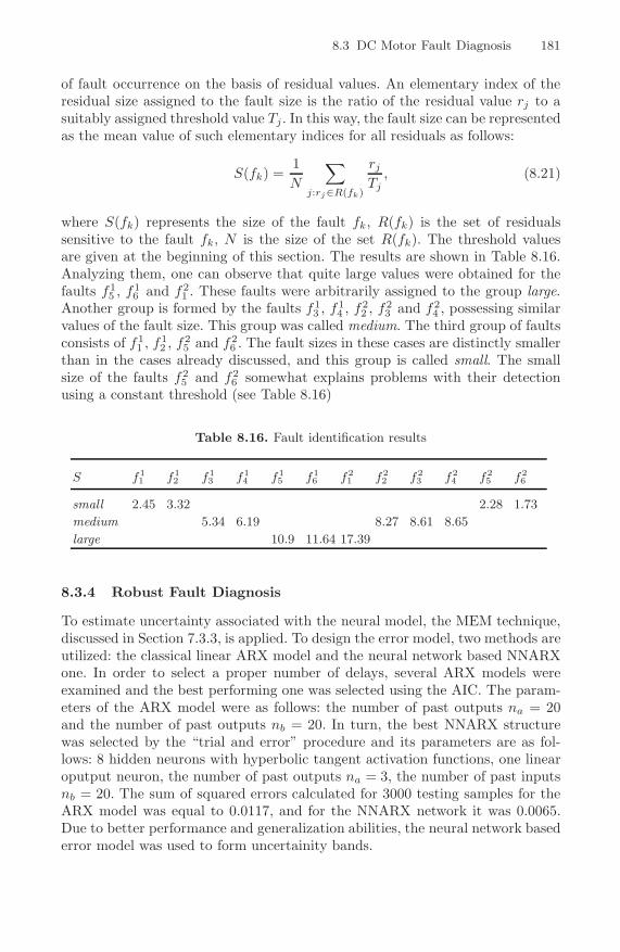
8.3 DC Motor Fault Diagnosis 181
of fault occurrence on the basis of residual values. An elementary index of theresidual size assigned to the fault size is the ratio of the residual value rj to asuitably assigned threshold value Tj. In this way, the fault size can be representedas the mean value of such elementary indices for all residuals as follows:
S(fk) =1N
∑j:rj∈R(fk)
rj
Tj, (8.21)
where S(fk) represents the size of the fault fk, R(fk) is the set of residualssensitive to the fault fk, N is the size of the set R(fk). The threshold valuesare given at the beginning of this section. The results are shown in Table 8.16.Analyzing them, one can observe that quite large values were obtained for thefaults f1
5 , f16 and f2
1 . These faults were arbitrarily assigned to the group large.Another group is formed by the faults f1
3 , f14 , f2
2 , f23 and f2
4 , possessing similarvalues of the fault size. This group was called medium. The third group of faultsconsists of f1
1 , f12 , f2
5 and f26 . The fault sizes in these cases are distinctly smaller
than in the cases already discussed, and this group is called small. The smallsize of the faults f2
5 and f26 somewhat explains problems with their detection
using a constant threshold (see Table 8.16)
Table 8.16. Fault identification results
S f11 f1
2 f13 f1
4 f15 f1
6 f21 f2
2 f23 f2
4 f25 f2
6
small 2.45 3.32 2.28 1.73
medium 5.34 6.19 8.27 8.61 8.65
large 10.9 11.64 17.39
8.3.4 Robust Fault Diagnosis
To estimate uncertainty associated with the neural model, the MEM technique,discussed in Section 7.3.3, is applied. To design the error model, two methods areutilized: the classical linear ARX model and the neural network based NNARXone. In order to select a proper number of delays, several ARX models wereexamined and the best performing one was selected using the AIC. The param-eters of the ARX model were as follows: the number of past outputs na = 20and the number of past outputs nb = 20. In turn, the best NNARX structurewas selected by the “trial and error” procedure and its parameters are as fol-lows: 8 hidden neurons with hyperbolic tangent activation functions, one linearoputput neuron, the number of past outputs na = 3, the number of past inputsnb = 20. The sum of squared errors calculated for 3000 testing samples for theARX model was equal to 0.0117, and for the NNARX network it was 0.0065.Due to better performance and generalization abilities, the neural network basederror model was used to form uncertainity bands.
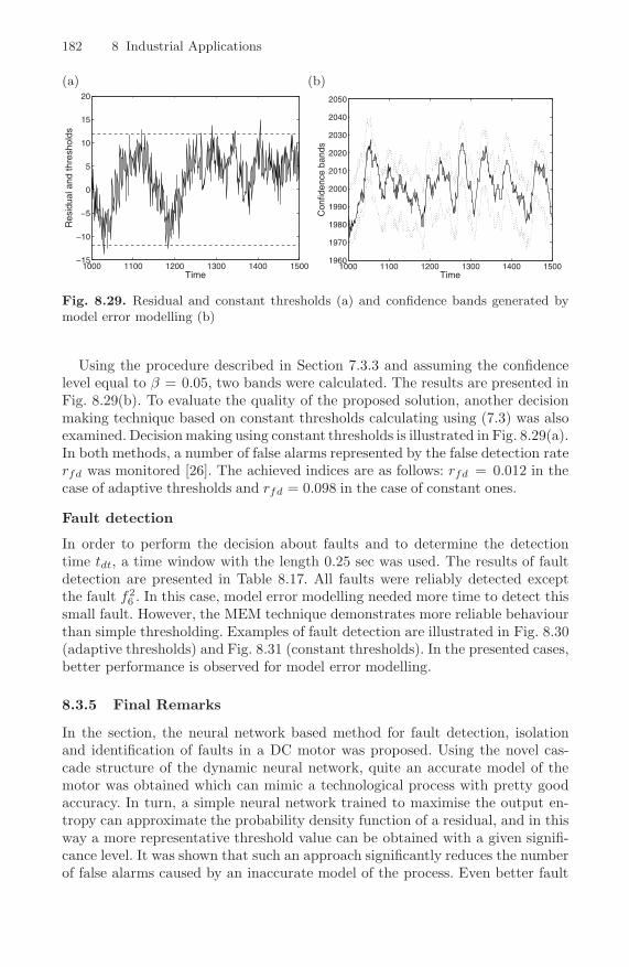
182 8 Industrial Applications
(a) (b)
1000 1100 1200 1300 1400 1500−15
−10
−5
0
5
10
15
20
Time
Res
idua
l and
thre
shol
ds
1000 1100 1200 1300 1400 15001960
1970
1980
1990
2000
2010
2020
2030
2040
2050
Time
Con
fiden
ce b
ands
Fig. 8.29. Residual and constant thresholds (a) and confidence bands generated bymodel error modelling (b)
Using the procedure described in Section 7.3.3 and assuming the confidencelevel equal to β = 0.05, two bands were calculated. The results are presented inFig. 8.29(b). To evaluate the quality of the proposed solution, another decisionmaking technique based on constant thresholds calculating using (7.3) was alsoexamined. Decision making using constant thresholds is illustrated in Fig. 8.29(a).In both methods, a number of false alarms represented by the false detection raterfd was monitored [26]. The achieved indices are as follows: rfd = 0.012 in thecase of adaptive thresholds and rfd = 0.098 in the case of constant ones.
Fault detection
In order to perform the decision about faults and to determine the detectiontime tdt, a time window with the length 0.25 sec was used. The results of faultdetection are presented in Table 8.17. All faults were reliably detected exceptthe fault f2
6 . In this case, model error modelling needed more time to detect thissmall fault. However, the MEM technique demonstrates more reliable behaviourthan simple thresholding. Examples of fault detection are illustrated in Fig. 8.30(adaptive thresholds) and Fig. 8.31 (constant thresholds). In the presented cases,better performance is observed for model error modelling.
8.3.5 Final Remarks
In the section, the neural network based method for fault detection, isolationand identification of faults in a DC motor was proposed. Using the novel cas-cade structure of the dynamic neural network, quite an accurate model of themotor was obtained which can mimic a technological process with pretty goodaccuracy. In turn, a simple neural network trained to maximise the output en-tropy can approximate the probability density function of a residual, and in thisway a more representative threshold value can be obtained with a given signifi-cance level. It was shown that such an approach significantly reduces the numberof false alarms caused by an inaccurate model of the process. Even better fault

8.3 DC Motor Fault Diagnosis 183
(a) (b)
3700 3800 3900 4000 4100 4200 4300 44001800
1850
1900
1950
2000
2050
Time
Con
fiden
ce b
ands
3700 3800 3900 4000 4100 4200 4300 4400−0.5
0
0.5
1
1.5
Time
Dec
isio
n m
akin
g
(c) (d)
3700 3800 3900 4000 4100 4200 4300 44001800
1900
2000
2100
2200
2300
2400
2500
2600
Time
Con
fiden
ce b
ands
3700 3800 3900 4000 4100 4200 4300 4400−0.5
0
0.5
1
1.5
Time
Dec
isio
n m
akin
g
(e) (f)
3700 3800 3900 4000 4100 4200 4300 44001940
1960
1980
2000
2020
2040
2060
2080
2100
2120
2140
Time
Con
fiden
ce b
ands
3700 3800 3900 4000 4100 4200 4300 4400−0.5
0
0.5
1
1.5
Time
Dec
isio
n m
akin
g
Fig. 8.30. Fault detection using model error modelling: fault f11 – confidence bands
(a) and decision logic without the time window (b); fault f16 – confidence bands (c)
and decision logic without the time window (d); fault f24 – confidence bands (e) and
decision logic without the time window (f)

184 8 Industrial Applications
(a) (b)
3700 3800 3900 4000 4100 4200 4300 4400−70
−60
−50
−40
−30
−20
−10
0
10
20
Time
Res
idua
l and
thre
shol
ds
3700 3800 3900 4000 4100 4200 4300 4400−0.5
0
0.5
1
1.5
Time
Dec
isio
n m
akin
g(c) (d)
3700 3800 3900 4000 4100 4200 4300 4400−50
0
50
100
150
200
250
300
Time
Res
idua
l and
thre
shol
ds
3700 3800 3900 4000 4100 4200 4300 4400−0.5
0
0.5
1
1.5
Time
Dec
isio
n m
akin
g
(e) (f)
3700 3800 3900 4000 4100 4200 4300 4400−200
−150
−100
−50
0
50
Time
Res
idua
l and
thre
shol
ds
3700 3800 3900 4000 4100 4200 4300 4400−0.5
0
0.5
1
1.5
Time
Dec
isio
n m
akin
g
Fig. 8.31. Fault detection by using constant thresholds: fault f11 – residual with thresh-
olds (a) and decision logic without the time window (b); fault f16 – residual with
thresholds (c) and decision logic without the time window (d); fault f24 – residual with
thresholds (e) and decision logic without the time window (f)

8.3 DC Motor Fault Diagnosis 185
Table 8.17. Results of fault detection for model error modelling
f11 f1
2 f13 f1
4 f15 f1
6
Model error modelling
rtd [%] 97.9 99.6 98.8 99.7 99.6 99.5
tdt 4074 4055 4077 4053 4058 4075
Constant thresholds
rtd [%] 98.1 99.4 98.8 99.4 98.9 100
tdt 4072 4067 4064 3147 4063 4018
f21 f2
2 f23 f2
4 f25 f2
6
Model error modelling
rtd [%] 99.2 99.3 99.2 98.8 99.1 81
tdt 4058 4100 4060 4061 4060 4357
Constant thresholds
rtd [%] 99.5 99.7 99.3 99.1 99.9 98.4
tdt 4056 4059 4057 4059 3726 3132
detection results can be obtained by means of robust fault diagnosis carried outusing model error modelling. Due to the estimation of model uncertainty, therobust fault diagnosis system may be much more sensitive to the occurrence ofsmall faults than standard decision making methods such as constant thresholds.The supremacy of MEM may be evident in the case of incipient faults, when afault develops very slowly and a robust technique performs in a more sensitivemanner that constant thresholds. Moreover, comparing the false detection ra-tios calculated for normal operating conditions for adaptive as well as constantthresholds, one can conclude that the number of false alarms was considerablyreduced when model error modelling was applied. Furhermore, fault isolationwas performed using the standard multi-layer perceptron. Preliminary analysisof the symptom distribution and splitting faulty scenarios into groups make itpossible to obtain high fault isolation rates. The last step in the fault diagno-sis procedure was fault identification. In the framework of fault identification,the objective was to estimate the fault size. The size of a fault was estimated bychecking how much the residual exceeded the threshold assigned to it. The wholefault diagnosis approach was successfully tested on a number of faulty scenariossimulated in the real plant, and the achieved results confirm the usefulness andeffectiveness of artificial neural networks in designing fault detection and isola-tion systems. It should be pointed out that the presented solution can be easilyapplied to on-line fault diagnosis.

9 Concluding Remarks and Further ResearchDirections
There is no doubt that artificial neural networks have gained a considerable posi-tion in the existing state-of-the-art in the field of both the modelling and identifi-cation of non-linear dynamic processes and fault diagnosis of technical processes.The self-learning ability and the property of approximating non-linear functionsprovide the modelling of non-linear systems with a great flexibility. These fea-tures allow one to design adaptive control systems for complex, unknown andnon-linear dynamic processes. The present monograph is mainly devoted to aspecial class of dynamically driven neural networks consisting of neuron modelswith IIR filters. The existing literature shows a great potential of locally recur-rent globally feedforward networks, which is confirmed by a variety of applica-tions in different scietific areas. Therefore, the application of locally recurrentnetworks to the modelling of technical processes and fault diagnosis seems to bejustified.
In the light of the discussion above, the original objective of the research re-ported in this monograph was to develop efficient tools able to solve problemsencountered in modelling and identification theory, and model based fault di-agnosis. In order to accomplish this task, appropriate theoretical deliberationswere carried out. Furhermore, some known methods were generalized and sev-eral new algorithms were constructed. The following is a concise summary ofthe original contributions provided by this monograph to the state-of-the-art inneural network modelling and fault diagnosis of non-linear dynamic processes:
• Detailed analysis of dynamic properties of the neuron model with the IIRfilter including the analysis of the equilibrium points, observability and con-trolability. Deriving state-space representations of locally recurrent globallyfeedforward neural networks with one and two hidden layers needed in bothstability and approximation discussions. Deriving training algorithms basedon global optimisation techniques in order to obtain a high quality model ofa given process;
• Formulating stability conditions for LRGF networks. Based on the conditionsobtained for the LRGF network with one hidden layer, a stabilization problemwas defined and solved as a constrained optimisation task. For the LRGF
K. Patan: Artificial. Neural Net. for the Model. & Fault Diagnosis, LNCIS 377, pp. 187–189, 2008.springerlink.com c© Springer-Verlag Berlin Heidelberg 2008

188 9 Concluding Remarks and Further Research Directions
network with two hidden layers, both local and global stability conditionswere derived using Lyapunov’s methods. Global stability conditions wereformulated in the form of LMIs, which makes checking the stability very easy.Based on local stability conditions, constraints on the network parameterswere defined. Thus, a constrained training algorithm was elaborated whichguarantees the stability of the neural model;
• Proving approximation abilities of LRGF networks. In the monograph it wasproved that the locally recurrent network with two hidden layers is able toapproximate a state-space trajectory produced by any Lipschitz continuousfunction with arbitrary accuracy. The undertaken analysis of the discussednetwork rendered it possible to simplify its structure and to significantly re-duce the number of parameters. Thus, a novel structure of a locally recurrentneural network was proposed;
• Developing methods for optimal training sequence selection for dynamicneural networks. The result presented in the monograph is in fact the firststep to the problem which, in the author’s opinion, is the most challengingone among these stated in the monograph. To solve this problem, some well-known methods of optimum experimental design for linear regression modelswere successfully adopted;
• Technical and industrial applications. Three applications were discussed:
– application of the discussed approaches to the modelling and fault detec-tion and isolation of the components of a sugar evaporator based on realprocess data,
– application of the investigated approaches to the modelling and fault de-tection of the components of a fluid catalytic cracking converter simulator.
– application of the developed approaches to the modelling and fault detec-tion, isolation and identification of an electrical drive laboratory system.
Moreover, the uncertainty of the neural model in the framework of faultdiagnosis was investigated. In the monograph, the model error modellingmethod was extended to the time domain. Moreover, the neural version ofthis method was proposed.
From the engineering point of view, many of the proposed approaches lead tomore transparent solutions aa well as many efficient and easy to implement nu-merical procedures. The author strongly believes that these advantages establisha firm position of the discussed methodologies regarding applications in widelyunderstood engineering. Neverthless, there still remain open problems, whichrequire closer attention and indicate further research directions. In particular,the following research problems should be considerd:
• to determine an appropriate number of hidden neurons, which assure therequired level of approximation accuracy,
• to select the proper order of filters to capture the dynamics of the modelledprocess,
• to propose new Lyapunov candidate functions, which make it possible toformulate less restrictive stability conditions,

9 Concluding Remarks and Further Research Directions 189
• to investigate more robust procedures for stabilizing neural networks duringtraining, which will deteriorate the training process in a negligible way,
• to find a proper structure of the error model in order to obtain a very sensitiverobust fault detection procedure,
• to propose fault models using dynamic neural networks without the need forfaulty data,
• to integrate neural network based fault diagnosis with the fault tolerant con-trol system.

References
1. Sorsa, T., Koivo, H.N.: Application of neural networks in the detection of breaksin a paper machine. In: Preprints IFAC Symp. On-line Fault Detection andSupervision in the Chemical Process Industries, Newark, Delaware, USA. (1992)162–167
2. Himmelblau, D.M.: Use of artificial neural networks in monitor faults and fortroubleshooting in the process industries. In: Preprints IFAC Symp. On-line FaultDetection and Supervision in the Chemical Process Industries, Newark, Delaware,USA. (1992) 144–149
3. Patton, R.J., Chen, J., Siew, T.: Fault diagnosis in nonlinear dynamic systemsvia neural networks. In: Proc. of CONTROL’94, Coventry, UK. Volume 2. (1994)1346–1351
4. Frank, P.M., Koppen-Seliger, B.: New developments using AI in fault diagnosis.Engineering Applications of Artificial Intelligence 10 (1997) 3–14
5. Patton, R.J., Korbicz, J.: Advances in computational intelligence. Special Issueof International Journal of Applied Mathematics and Computer Science 9 (1999)
6. Calado, J., Korbicz, J., Patan, K., Patton, R., Sa da Costa, J.: Soft computingapproaches to fault diagnosis for dynamic systems. European Journal of Control7 (2001) 248–286
7. Korbicz, J., Koscielny, J., Kowalczuk, Z., Cholewa, W.: Fault Diagnosis. Models,Artificial Intelligence, Applications. Springer-Verlag, Berlin Heidelberg (2004)
8. Isermann, R.: Supervision, fault detection and diagnosis of technical systems.Special Section of Control Engineering Practice 5 (1997)
9. Chen, J., Patton, R.J.: Robust Model-Based Fault Diagnosis for Dynamic Sys-tems. Kluwer Academic Publishers, Berlin (1999)
10. Patton, R.J., Frank, P.M., Clark, R.: Issues of Fault Diagnosis for DynamicSystems. Springer-Verlag, Berlin (2000)
11. Korbicz, J., Patan, K., Kowal, M., eds.: Fault Diagnosis and Fault TolerantControl. Challenging Problems of Science - Theory and Applications : AutomaticControl and Robotics. Academic Publishing House EXIT, Warsaw (2007)
12. Witczak, M.: Modelling and Estimation Strategies for Fault Diagnosis of Non-Linear Systems. From Analytical to Soft Computing Approaches. Lecture Notesin Control and Information Sciences. Springer–Verlag, Berlin (2007)
13. Isermann, R.: Fault diagnosis of machines via parameter estimation and knowl-edge processing – A tutorial paper. Automatica 29 (1994) 815–835

192 References
14. Patton, R.J., Frank, P.M., Clark, R.N.: Issues of Fault Diagnosis for DynamicSystems. Springer-Verlag, Berlin (2000)
15. Gertler, J.: Fault Detection and Diagnosis in Engineering Systems. Marcel Dekker,Inc., New York (1998)
16. Isermann, R.: Fault Diagnosis Systems. An Introduction from Fault Detection toFault Tolerance. Springer-Verlag, New York (2006)
17. Rutkowski, L.: New Soft Computing Techniques for System Modelling, PatternClassification and Image Processing. Springer-Verlag, Berlin (2004)
18. Nelles, O.: Nonlinear System Identification. From Classical Approaches to NeuralNetworks and Fuzzy Models. Springer-Verlag, Berlin (2001)
19. Norgard, M., Ravn, O., Poulsen, N., Hansen, L.: Networks for Modelling andControl of Dynamic Systems. Springer-Verlag, London (2000)
20. Narendra, K.S., Parthasarathy, K.: Identification and control of dynamical sys-tems using neural networks. IEEE Transactions on Neural Networks 1 (1990)12–18
21. Hunt, K.J., Sbarbaro, D., Zbikowski, R., Gathrop, P.J.: Neural networks forcontrol systems. – A survey. Automatica 28 (1992) 1083–1112
22. Miller, W.T., Sutton, R.S., Werbos, P.J.: Neural Networks for Control. MITPress, Cambridge, MA (1990)
23. Haykin, S.: Neural Networks. A Comprehensive Foundation, 2nd Edition.Prentice-Hall, New Jersey (1999)
24. Zhang, J., Man, K.F.: Time series prediction using RNN in multi-dimensionembedding phase space. In: Proc. IEEE Int. Conf. Systems, Man and Cybernetics,San Diego, USA, 11–14 October. (1998) 1868–1873 Published on CD-ROM.
25. Janczak, A.: Identification of Nonlinear Systems Using Neural Networks andPolynomial Models. A Block-oriented Approach. Lecture Notes in Control andInformation Sciences. Springer–Verlag, Berlin (2005)
26. Patan, K., Parisini, T.: Identification of neural dynamic models for fault detectionand isolation: The case of a real sugar evaporation process. Journal of ProcessControl 15 (2005) 67–79
27. Guglielmi, G., Parisini, T., Rossi, G.: Fault diagnosis and neural networks: Apower plant application (keynote paper). Control Engineering Practice 3 (1995)601–620
28. Osowski, S.: Neural Networks in Algorithmitic Expression. WNT, Warsaw (1996)(in Polish).
29. Hertz, J., Krogh, A., Palmer, R.G.: Introduction to the Theory of Neural Com-putation. Addison-Wesley Publishing Company, Inc. (1991)
30. Looney, C.G.: Pattern Recognition Using Neural Networks. Oxford UniversityPress (1997)
31. Sharkey, A.J.C., ed.: Combining Artificial Neural Nets. Springer-Verlag, London,UK (1999)
32. Hornik, K., Stinchcombe, M., White, H.: Multilayer feedforward networks areuniversal approximators. Neural Networks 2 (1989) 359–366
33. Cybenko, G.: Approximation by superpositions of a sigmoidal function. Mathe-matics of Control, Signals, and Systems 2 (1989) 303–314
34. Kuschewski, J.G., Hui, S., Zak, S.: Application of feedforward neural networksto dynamical system identification and control. IEEE Transactions on NeuralNetworks 1 (1993) 37–49
35. Williams, R.J., Zipser, D.: A learning algorithm for continually running fullyrecurrent neural networks. Neural Computation 1 (1989) 270–289

References 193
36. Elman, J.L.: Finding structure in time. Cognitive Science 14 (1990) 179–21137. Parlos, A.G., Chong, K.T., Atiya, A.F.: Application of the recurrent multilayer
perceptron in modelling complex process dynamics. IEEE Transactions on NeuralNetworks 5 (1994) 255–266
38. Tsoi, A.C., Back, A.D.: Locally recurrent globally feedforward networks: A criticalreview of architectures. IEEE Transactions on Neural Networks 5 (1994) 229–239
39. Marcu, T., Mirea, L., Frank, P.M.: Development of dynamical neural networkswith application to observer based fault detection and isolation. InternationalJournal of Applied Mathematics and Computer Science 9 (1999) 547–570
40. Campolucci, P., Uncini, A., Piazza, F., Rao, B.D.: On-line learning algorithmsfor locally recurrent neural networks. IEEE Transactions on Neural Networks 10(1999) 253–271
41. Korbicz, J., Patan, K., Obuchowicz, A.: Neural network fault detection systemfor dynamic processes. Bulletin of the Polish Academy of Sciences, TechnicalSciences. 49 (2001) 301–321
42. Patan, K., Parisini, T.: Stochastic learning methods for dynamic neural net-works: Simulated and real-data comparisons. In: Proc. 2002 American ControlConference, ACC’02. Anchorage, Alaska, USA, May 8–10. (2002) 2577–2582
43. Patan, K., Parisini, T.: Stochastic approaches to dynamic neural network training.Actuator fault diagnosis study. In: Proc. 15th IFAC Triennial World Congress,b’02. Barcelona, Spain, July 21–26. (2002) Published on CD-ROM.
44. Patan, K., Korbicz, J.: Artificial neural networks in fault diagnosis. In Korbicz,J., Koscielny, J.M., Kowalczuk, Z., Cholewa, W., eds.: Fault Diagnosis. Models,Artificial Intelligence, Applications. Springer-Verlag, Berlin (2004) 330–380
45. Patan, K.: Training of the dynamic neural networks via constrained optimization.In: Proc. IEEE Int. Joint Conference on Neural Networks, IJCNN 2004, Budapest,Hungary. (2004) Published on CD-ROM.
46. Patan, K.: Approximation ability of a class of locally recurrent globally feed-forward neural networks. In: Proc. European Control Conference, ECC 2007,Kos, Greece, July 2–5. (2007) Published on CD-ROM.
47. Patan, K.: Aproximation of state-space trajectories by locally recur-rent globally feed-forward neural networks. Neural Networks (2007) DOI:10.1016/j.neunet.2007.10.004.
48. Patan, K., Korbicz, J., Pretki, P.: Global stability conditions of locally recurrentneural networks. Lecture Notes on Computer Science. Artificial Neural Networks:Formal Models and Their Applications – ICANN 2005 3697 (2005) 191–196
49. Patan, K.: Stability analysis and the stabilization of a class of discrete-timedynamic neural networks. IEEE Transactions on Neural Networks 18 (2007)660–673
50. Patan, K., Korbicz, J.: Fault detection in catalytic cracking converter by meansof probability density approximation. In: Proc. Int. Symp. Fault Detection Su-pervision and Safety for Technical Processes, SAFEPROCESS 2006, Beijing, P.R.China. (2006) Published on CD-ROM.
51. Patan, K., Korbicz, J., G�lowacki, G.: DC motor fault diagnosis by means ofartificial neural networks. In: Proc. 4th International Conference on Informaticsin Control, Automation and Robotics, ICINCO 2007, Angers, France, May 9–12.(2007) Published on CD-ROM.
52. Patan, K., Korbicz, J.: Fault detection in catalytic cracking converter by meansof probability density approximation. Engineering Applications of Artificial In-telligence 20 (2007) 912–923
194 References
53. Patan, M., Patan, K.: Optimal observation strategies for model-based fault detec-tion in distributed systems. International Journal of Control 78 (2005) 1497–1510
54. Patan, K.: Fault detection system for the sugar evaporator based on AI tech-niques. In: Proc. 6th IEEE Int. Conf. Methods and Models in Automation andRobotics, MMAR 2000. Miedzyzdroje, Poland, 28-21 August. (2000) 807–812
55. Patan, K.: Robust fault diagnosis in catalytic cracking converter using artificialneural networks. In: Proc. 16th IFAC World Congress, July 3-8, Prague, CzechRepublic. (2005) Published on CD-ROM.
56. Patan, K.: Robust faul diagnosis in a DC motor by means of artificial neuralnetworks and model error modelling. In Korbicz, J., Patan, K., Kowal, M., eds.:Fault Diagnosis and Fault Tolerant Control. Academic Publishing House Exit,Warsaw (2007) 337–346
57. Patan, K., Parisini, T.: Dynamic neural networks for actuator fault diagnosis:Application to DAMADICS benchmark problem. In: Proc. Int. Symp. FaultDetection Supervision and Safety for Technical Processes, SAFEPROCESS 2003,Washington D.C., USA. (2003) Published on CD-ROM.
58. Patan, K.: Fault detection of the actuators using neural networks. In: Proc. 7thIEEE Int. Conf. Methods and Models in Automation and Robotics, MMAR 2001.Miedzyzdroje, Poland, August 28–31. Volume 2. (2001) 1085–1090
59. Patan, K.: Actuator fault diagnosis study using dynamic neural networks. In:Proc. 8th IEEE Int. Conf. Methods and Models in Automation and Robotics,MMAR 2002. Szczecin, Poland, September 2–5. (2002) 219–224
60. Gertler, J.: Analytical redundancy methods in fault detection and isolation. Sur-vey and synthesis. In: Proc. Int. Symp. Fault Detection Supervision and Safety forTechnical Processes, SAFEPROCESS’91, Baden-Baden, Germany. (1991) 9–21
61. Koscielny, J.M.: Diagnostics of Automatic Industrial Processes. Academic Pub-lishing Office EXIT (2001) (in Polish).
62. Liu, M., Zang, S., Zhou, D.: Fast leak detection and location of gas pipelines basedon an adaptive particle filter. International Journal of Applied Mathematics andComputer Science 15 (2005) 541–550
63. Koscielny, J.M.: Fault isolation in industrial processes by dynamic table of statesmethod. Automatica 31 (1995) 747–753
64. Koppen-Seliger, B., Frank, P.M.: Fuzzy logic and neural networks in fault detec-tion. In Jain, L., Martin, N., eds.: Fusion of Neural Networks, Fuzzy Sets, andGenetic Algorithms, New York, CRC Press (1999) 169–209
65. Patton, R.J., Frank, P.M., Clark, R.N., eds.: Fault Diagnosis in Dynamic Systems.Theory and Application. Prentice Hall, New York (1989)
66. Walter, E., Pronzato, L.: Identification of Parametric Models from ExperimentalData. Springer, London (1997)
67. Soderstrom, T., Stoica, P.: System Identification. Prentice-Hall International,Hemel Hempstead (1989)
68. Milanese, M., Norton, J., Piet-Lahanier, H., Walter, E.: Bounding Approaches toSystem Identification. Plenum Press, New York (1996)
69. Isermann, R.: Fault diagnosis of machines via parameter estimation and knowl-edge processing. Automatica 29 (1993) 815–835
70. Walker, B.K., Kuang-Yang, H.: FDI by extended Kalman filter parameter es-timation for an industrial actuator benchmark. Control Engineering Practice 3(1995) 1769–1774
71. Massoumnia, B.K., Vander Velde, W.E.: Generating parity relations for detectingand identifying control system components failures. Journal of Guidance, Controland Dynamics 11 (1988) 60–65

References 195
72. Peng, Y.B., Youssouf, A., Arte, P., Kinnaert, M.: A complete procedure forresidual generation and evaluation with application to a heat exchanger. IEEETransactions on Control Systems Technology 5 (1997) 542–555
73. Guernez, C., Cassar, J.P., Staroswiecki, M.: Extension of parity space to non-linear polynomial dynamic systems. In: Proc. 3rd IFAC Symp. Fault Detection,Supervision and Safety of Technical Processes, SAFEPROCESS’97, Hull, UK.Volume 2. (1997) 861–866
74. Krishnaswami, V., Rizzoni, G.: Non-linear parity equation residual generationfor fault detection and isolation. In Ruokonen, T., ed.: Proc. IFAC SymposiumSAFEPROCESS’94, Espoo, Finland. Volume 1., Pergamon Press (1994) 317–332
75. Anderson, B.D.O., Moore, J.B.: Optimal Filtering. Prentice-Hall, New Jersey(1979)
76. Hui, S., Zak, S.H.: Observer design for systems with unknown inputs. Interna-tional Journal of Applied Mathematics and Computer Science 15 (2005) 431–446
77. Gupta, M.M., Jin, L., Homma, N.: Static and Dynamic Neural Networks. FromFundamentals to Advanced Theory. John Wiley & Sons, New Jersey (2003)
78. Kowalski, C.T.: Monitoring and Fault Diagnosis of Induction Motors Using NeuralNetworks. Wroc�law University of Technology Academic Press, Wroc�law, Poland(2005) (in Polish).
79. Tadeusiewicz, R.: Neural Networks. Academic Press RM, Warsaw (1993) (inPolish).
80. Koivo, M.H.: Artificial neural networks in fault diagnosis and control. ControlEngineering Practice 2 (1994) 89–101
81. Korbicz, J., Mrugalski, M.: Confidence estimation of GMDH neural networksand its application in fault detection systems. International Journal of SystemsScience (2007) DOI: 10.1080/00207720701847745.
82. Babuka, R.: Fuzzy Modeling for Control. Kluwer Academic Publishers, London(1998)
83. Jang, J.: ANFIS: Adaptive-network-based fuzzy inference system. IEEE Trans-actions on Systems, Man and Cybernetics 23 (1995) 665–685
84. Rutkowska, D.: Neuro-Fuzzy Architectures and Hybrid Learning. Springer, Berlin(2002)
85. Osowski, S., Tran Hoai, L., Brudzewski, K.: Neuro-fuzzy TSK network for cali-bration of semiconductor sensor array for gas measurements. IEEE Transactionson Measurements and Instrumentation 53 (2004) 630–637
86. Kowal, M.: Optimization of Neuro-Fuzzy Structures in Technical Diagnostic Sys-tems. Volume 9 of Lecture Notes in Control and Computer Science. Zielona GoraUniversity Press, Zielona Gora, Poland (2005)
87. Korbicz, J., Kowal, M.: Neuro-fuzzy networks and their application to fault de-tection of dynamical systems. Engineering Applications of Artificial Intelligence20 (2007) 609–617
88. Widrow, B., Hoff, M.E.: Adaptive switching circuit. In: 1960 IRE WESCONConvention Record, part 4, New York, IRE (1960) 96–104
89. Widrow, B.: Generalization and information storage in networks of adaline neu-rons. In Yovits, M., Jacobi, G.T., Goldstein, G., eds.: Self-Organizing Systems1962 (Chicago 1962), Washington, Spartan (1962) 435–461
90. Duch, W., Korbicz, J., Rutkowski, L., Tadeusiewicz, R., eds.: Biocyberneticsand Biomedical Engineering 2000. Neural Networks. Academic Publishing OfficeEXIT, Warsaw (2000) (in Polish).
91. Werbos, P.J.: Beyond Regression: New Tools for Prediction and Analysis in theBehavioral Sciences. PhD thesis, Harvard University (1974)

196 References
92. Rumelhart, D.E., Hinton, G.E., Williams, R.J.: Learning representations by back-propagating errors. Nature (1986) 533–536
93. Rumelhart, D.E., Hinton, G.E., Williams, R.J.: Learning internal representationsby error propagation. Parallel Distributed Processing I (1986)
94. Plaut, D., Nowlan, S., Hinton, G.: Experiments of learning by back propagation.Technical Report CMU-CS-86-126, Department of Computer Science, CarnegieMelon University, Pittsburg, PA (1986)
95. Demuth, H., Beale, M.: Neural Network Toolbox for Use with MATLAB. TheMathWorks Inc. (1993)
96. Fahlman, S.E.: Fast learning variation on back-propagation: An empirical study.In Touretzky, D., Hilton, G., Sejnowski, T., eds.: Proceedings of the 1988 Connec-tionist Models Summer School (Pittsburg 1988), San Mateo, Morgan Kaufmann(1989) 38–51
97. Fahlman, S.E., Lebiere, C.: The cascade-correlation learning architecture. InTouretzky, D.S., ed.: Advances in Neural Information Processing Systems II (Den-ver 1989), San Mateo, Morgan Kaufmann (1990) 524–532
98. Rojas, R.: Neural Networks. A Systematic Introduction. Springer-Verlag, Berlin(1996)
99. Hagan, M.T., Menhaj, M.B.: Training feedforward networks with the Marquardtalgorithm. IEEE Transactions on Neural Networks 5 (1994) 989–993
100. Hagan, M., Demuth, H.B., Beale, M.H.: Neural Network Design. PWS Publishing,Boston, MA (1996)
101. Girosi, J., Poggio, T.: Neural networks and the best approximation property.Biol. Cybernetics 63 (1990) 169–176
102. Park, J., Sandberg, I.W.: Universal approximation using radial-basis-functionnetworks. Neural Computation 3 (1991) 246–257
103. Chen, S., Billings, S.A.: Neural network for nonliner dynamic system modellingand identification. International Journal of Control 56 (1992) 319–346
104. Warwick, K., Kambhampati, C., Parks, P., Mason, J.: Dynamic systems in neuralnetworks. In Hunt, K.J., Irwin, G.R., Warwick, K., eds.: Neural Network Engi-neering in Dynamic Control Systems, Berlin, Springer-Verlag (1995) 27–41
105. Chen, S., Cowan, C.F.N., Grant, P.M.: Orthogonal least squares learning algo-rithm for radial basis function networks. IEEE Transactions on Neural Networks2 (1991) 302–309
106. Kohonen, T.: Self-organization and Associative Memory. Springer-Verlag, Berlin(1984)
107. Zhou, Y., Hahn, J., Mannan, M.S.: Fault detection and classification in chemicalprocesses based on neural networks with feature extraction. ISA Transactions 42(2003) 651–664
108. Chen, Y.M., Lee, M.L.: Neural networks-based scheme for system failure detectionand diagnosis. Mathematics and Computers in Simulation 58 (2002) 101–109
109. Ayoubi, M.: Fault diagnosis with dynamic neural structure and application toa turbo-charger. In: Proc. Int. Symp. Fault Detection Supervision and Safetyfor Technical Processes, SAFEPROCESS’94, Espoo, Finland. Volume 2. (1994)618–623
110. Zhang, J., Roberts, P.D., Ellis, J.E.: A self-learning fault diagnosis system. Trans-actions of the Institute of Measurements and Control 13 (1991) 29–35
111. Karhunen, J.: Optimization criteria and nonlinear PCA neural networks. In:Proc. Int. Conf. Neural Networks, ICNN. (1994) 1241–1246

References 197
112. Karpenko, M., Sepehri, N., Scuse, D.: Diagnosis of process valve actuator faultsusing multilayer neural network. Control Engineering Practice 11 (2003) 1289–1299
113. Zhang, J.: Improved on-line process fault diagnosis through information fusion inmultiple neural networks. Computers & Chemical Engineering 30 (2006) 558–571
114. Xu, P., Xu, S., Yin, H.: Application of self-organizing competitive neural networkin fault diagnosis of suck rod pumping system. Journal of Petroleum Science &Engineering 58 (2006) 43–48
115. G�lowacki, G., Patan, K., Korbicz, J.: Nonlinear principal component analysisin fault diagnosis. In Korbicz, J., Patan, K., Kowal, M., eds.: Fault Diagnosisand Fault Tolerant Control, ISBN: 978-83-60434-32-1. Challenging Problems ofScience - Theory and Applications : Automatic Control and Robotics. AcademicPublishing House EXIT, Warsaw (2007) 211–218
116. Harkat, M.F., Djelel, S., Doghmane, N., Benouaret, M.: Sensor of fault detec-tion, isolation and reconstruction using nonlinear principal component analysis.International Journal of Automation and Computing (2007) 149–155
117. Arbib, M.A., ed.: The Metaphorical Brain, 2nd edition. Wiley, New York (1989)118. Mozer, M.C.: Neural net architectures for temporal sequence processing. In
Weigend, A.S., A, G.N., eds.: Time series predictions: Forecasting the future andunderstanding the past, Reading, MA, Addison-Wesley Publishing Company, Inc.(1994) 243–264
119. Zamarreno, J.M., Vega, P.: State space neural network. Properties and applica-tion. Neural Networks 11 (1998) 1099–1112
120. Williams, R.J.: Adaptive state representation and estimation using recurrentconnectionist networks. In: Neural Networks for Control, London, MIT Press(1990) 97–115
121. Stornetta, W.S., Hogg, T., Hubermann, B.A.: A dynamic approach to tempo-ral pattern processing. In Anderson, D.Z., ed.: Neural Information ProcessingSystems, New York, American Institute of Physics (1988) 750–759
122. Mozer, M.C.: A focused backpropagation algorithm for temporal pattern recog-nition. Complex Systems 3 (1989) 349–381
123. Jordan, M.I., Jacobs, R.A.: Supervised learning and systems with excess degreesof freedom. In Touretzky, D.S., ed.: Advances in Neural Information ProcessingSystems II (Denver 1989), San Mateo, Morgan Kaufmann (1990) 324–331
124. Jordan, M.I.: Attractor dynamic and parallelism in a connectionist sequential ma-chine. In: Proc. 8th Annual Conference of the Cognitive Science Society (Amherst,1986), Hillsdale, Erlbaum (1986) 531–546
125. Anderson, S., Merrill, J.W.L., Port, R.: Dynamic speech categorization withrecurrent networks. In Touretzky, D., Hinton, G., Sejnowski, T., eds.: Proc. ofthe 1988 Connectionist Models Summer School (Pittsburg 1988), San Mateo,Morgan Kaufmann (1989) 398–406
126. Pham, D.T., Xing, L.: Neural Networks for Identification, Prediction and Control.Springer-Verlag, Berlin (1995)
127. Sontag, E.: Feedback stabilization using two-hidden-layer nets. IEEE Transac-tions on Neural Networks 3 (1992) 981–990
128. Gori, M., Bengio, Y., Mori, R.D.: BPS: A learning algorithm for capturing thedynamic nature of speech. In: International Joint Conference on Neural Networks.Volume II. (1989) 417–423
129. Back, A.D., Tsoi, A.C.: FIR and IIR synapses, A new neural network architecturefor time series modelling. Neural Computation 3 (1991) 375–385

198 References
130. Fasconi, P., Gori, M., Soda, G.: Local feedback multilayered networks. NeuralComputation 4 (1992) 120–130
131. Poddar, P., Unnikrishnan, K.P.: Memory neuron networks: A prolegomenon.Technical Report GMR-7493, General Motors Research Laboratories (1991)
132. Gupta, M.M., Rao, D.H.: Dynamic neural units with application to the controlof unknown nonlinear systems. Journal of Intelligent and Fuzzy Systems 1 (1993)73–92
133. Hopfield, J.: Neural networks and physical systems with emergent collective com-putational abilities. In: Proc. Nat. Acad. Sci. USA. (1982) 2554–2558
134. Pineda, F.J.: Dynamics and architecture for neural computation. J. Complexity4 (1988) 216–245
135. Pineda, F.J.: Generalization of back-propagation to recurrent neural networks.Physical Rev. Lett. 59 (1987) 2229–2232
136. Grossberg, S.: Content-addressable memory storage by neural networks: A gen-eral model and global Lyapunov method. In Schwartz, E.L., ed.: ComputationalNeuroscience, Cambridge, MA, MIT Press (1990)
137. Sastry, P.S., Santharam, G., Unnikrishnan, K.P.: Memory neuron networks foridentification and control of dynamical systems. IEEE Transactions on NeuralNetworks 5 (1994) 306–319
138. Zurada, J.M.: Lambda learning rule for feedforward neural networks. In: Proc.Int. Conf. on Neural Networks. San Francisco, USA, March 28–April 1. (1993)1808–1811
139. Horn, R.A., Johnson., C.R.: Matrix Analysis. Cambridge University Press, Cam-bridge (1985)
140. Klamka, J.: Stochastic controllability of linear systems with state delays. In-ternational Journal of Applied Mathematics and Computer Science 17 (2007)5–13
141. Oprzedkiewicz, K.: An observability problem for a class of uncertain-parameterlinear dynamic systems. International Journal of Applied Mathematics and Com-puter Science 15 (2005) 331–338
142. Vidyasagar, M.: Nonlinear System Analysis, 2nd edition. Prentice-Hall, Engle-wood Cliffs, NJ (1993)
143. Levin, A.U., Narendra, K.S.: Control of nonlinear dynamical systems using neuralnetworks: Controllability and stabilization. IEEE Transactions on Neural Net-works 4 (1993) 192–206
144. Patan, K., Korbicz, J.: Dynamic Networks and Their Application in Modellingand Identification. In Duch, W., Korbicz, J., Rutkowski, L., Tadeusiewicz, R.,eds.: Biocybernetics and Biomedical Engineering 2000. Neural Networks. Acad-emic Publishing Office EXIT, Warsaw (2000) (in Polish).
145. Spall, J.C.: Introduction to Stochastic Search and Optimization. John Willey &Sons, New Jersey (2003)
146. Pflug, G.C.: Optimization of Stochastic Models. The Interface Between Simula-tion and Optimization. Kluwer Academic Publishers, Boston (1996)
147. Spall, J.: Multivariate stochastic aproximation using a simultaneous perturbationgradient approximation. IEEE Transactions on Automatic Control (1992) 332–341
148. Spall, J.: Stochastic optimization, stochastic approximation and simulated anneal-ing. In Webster, J., ed.: Encyclopedia of Electrical and Electronics Engineering.John Wiley & Sons, New York (1999)
149. Spall, J.: Adaptive stochastic approximation by the simultaneous perturbationmethod. IEEE Transactions on Automatic Control 45 (2000) 1839–1853

References 199
150. Chin, D.C.: A more efficient global optimization algorithm based on Styblinskiand Tang. Neural Networks 7 (1994) 573–574
151. Maryak, J., Chin, D.C.: Global random optimization by simultaneous perturba-tion stochastic approximation. In: Proc. of the American Control Conference,ACC 2001, Arlington VA, USA. (2001) 756–762
152. Pham, D.T., Liu, X.: Training of Elman networks and dynamic system modelling.International Journal of Systems Science 27 (1996) 221–226
153. Lissane Elhaq, S., Giri, F., Unbehauen, H.: Modelling, identification and controlof sugar evaporation – theoretical design and experimental evaluation. ControlEngineering Practice (1999) 931–942
154. Cannas, B., Cincotti, S., Marchesi, M., Pilo, F.: Learnig of Chua’s circuit attrac-tors by locally recurrent neural networks. Chaos Solitons & Fractals 12 (2001)2109–2115
155. Zhang, J., Morris, A.J., Martin, E.B.: Long term prediction models based onmixed order locally recurrent neural networks. Computers Chem. Engng 22(1998) 1051–1063
156. Campolucci, P., Piazza, F.: Intrinsic stability-control method for recursive filtersand neural networks. IEEE Trans. Circuit and Systems – II: Analog and DigitalSignal Processing 47 (2000) 797–802
157. Jin, L., Nikiforuk, P.N., Gupta, M.M.: Approximation of discrete-time state-space trajectories using dynamic recurrent neural networks. IEEE Transactionson Automatic Control 40 (1995) 1266–1270
158. Garzon, M., Botelho, F.: Dynamical approximation by recurrent neural networks.Neurocomputing 29 (1999) 25–46
159. Leshno, M., Lin, V., Pinkus, A., Schoken, S.: Multilayer feedforward networkswith a nonpolynomial activation function can approximate any function. NeuralNetworks 6 (1993) 861–867
160. Scarselli, F., Tsoi, A.C.: Universal approximation using feedforward neural net-works: A survey of some existing methods, and some new results. Neural Networks11 (1998) 15–37
161. Hirsch, M., Smale, S.: Differential Equations, Dynamical Systems and LinearAlgebra. Academic Press, New York (1974)
162. Ljung, L.: System Identification – Theory for the User. Prentice Hall (1999)163. Matsuoka, K.: Stability conditions for nonlinear continuous neural networks with
asymmetric connection weights. Neural Networks 5 (1992) 495–500164. Ensari, T., Arik, S.: Global stability analysis of neural networks with multiple
time varying delays. IEEE Transactions on Automatic Control 50 (2005) 1781–1785
165. Liang, J., Cao, J.: A based-on LMI stability criterion for delayed recurrent neuralnetworks. Chaos, Solitons & Fractals 28 (2006) 154–160
166. Cao, J., Yuan, K., Li, H.: Global asymptotical stability of recurrent neural net-works with multiple discrete delays and distributed delays. IEEE Transactionson Neural Networks 17 (2006) 1646–1651
167. Forti, M., Nistri, P., Papini, D.: Global exponential stability and global conver-gence in finite time of delayed neural networks with infinite gain. IEEE Transac-tions on Neural Networks 16 (2005) 1449–1463
168. Fang, Y., Kincaid, T.G.: Stability analysis of dynamical neural networks. IEEETransactions on Neural Networks 7 (1996) 996–1006
169. Jin, L., Nikiforuk, P.N., Gupta, M.M.: Absolute stability conditions for discrete-time recurrent neural networks. IEEE Transactions on Neural Networks 5 (1994)954–963

200 References
170. Hu, S., Wang, J.: Global stability of a class of discrete-time recurrent neuralnetworks. IEEE Trans. Circuits and Systems – I: Fundamental Theory and Ap-plications 49 (2002) 1104–1117
171. Jin, L., Gupta, M.M.: Stable dynamic backpropagation learning in recurrentneural networks. IEEE Transactions on Neural Networks 10 (1999) 1321–1334
172. Suykens, J.A.K., Moor, B.D., Vandewalle, J.: Robust local stability of multilayerrecurrent neural networks. IEEE Transactions on Neural Networks 11 (2000)222–229
173. Kushner, H.J., Yin, G.G.: Stochastic Approximation Algorithms and Applica-tions. Springer-Verlag, New York (1997)
174. Paszke, W.: Analysis and Synthesis of Multidimensional System Classes usingLinear Matrix Inequality Methods. Volume 8 of Lecture Notes in Control andComputer Science. Zielona Gora University Press, Zielona Gora, Poland (2005)
175. Boyd S, L. E. Ghaoui, E.F., Balakrishnan, V.: Linear Matrix Inequalities in Sys-tem and Control Theory. SIAM Studies in Applied and Numerical Mathematics.SIAM, Philadelphia, USA (1994) Vol. 15.
176. Gahinet, P., Apkarian, P.: A linear matrix inequality approach to h∞ control.International Journal of Robust and Nonlinear Control 4 (1994) 421–448
177. Iwasaki, T., Skelton, R.E.: All controllers for the general H∞ control problem:LMI existence conditions and state space formulas. Automatica 30 (1994) 1307–1317
178. van de Wal, M., de Jager, B.: A review of methods for input/output selection.Automatica 37 (2001) 487–510
179. Fukumizu, K.: Statistical active learning in multilayer perceptrons. IEEE Trans-actions on Neural Networks 11 (2000) 17–26
180. Witczak, M.: Toward the training of feed-forward neural networks with the D-optimum input sequence. IEEE Transactions on Neural Networks 17 (2006) 357–373
181. Fedorov, V.V., Hackl, P.: Model-Oriented Design of Experiments. Lecture Notesin Statistics. Springer-Verlag, New York (1997)
182. Atkinson, A.C., Donev, A.N.: Optimum Experimental Designs. Clarendon Press,Oxford (1992)
183. Patan, M.: Optimal Observation Strategies for Parameter Estimation of Dis-tributed Systems. Volume 5 of Lecture Notes in Control and Computer Science.Zielona Gora University Press, Zielona Gora, Poland (2004)
184. Ucinski, D.: Optimal selection of measurement locations for parameter estima-tion in distributed processes. International Journal of Applied Mathematics andComputer Science 10 (2000) 357–379
185. Rafaj�lowicz, E.: Optimum choice of moving sensor trajectories for distributedparameter system identification. International Journal of Control 43 (1986) 1441–1451
186. Ucinski, D.: Optimal Measurement Methods for Distributed Parameter SystemIdentification. CRC Press, Boca Raton (2005)
187. Kiefer, J., Wolfowitz, J.: Optimum designs in regression problems. The Annalsof Mathematical Statistics 30 (1959) 271–294
188. Pazman, A.: Foundations of Optimum Experimental Design. Mathematics andIts Applications. D. Reidel Publishing Company, Dordrecht (1986)
189. Nyberg, M.: Model Based Fault Diagnosis: Methods, Theory, and AutomotiveEngine Applications. PhD thesis, Linkoping University, Linkoping, Sweden (1999)
190. Korbicz, J.: Robust fault detection using analytical and soft computing methods.Bulletin of the Polish Academy of Sciences, Technical Sciences 54 (2006) 75–88
References 201
191. Shumsky, A.: Redundancy relations for fault diagnosis in nonlinear uncertainsystems. International Journal of Applied Mathematics and Computer Science17 (2007) 477–489
192. Mrugalski, M., Witczak, M., Korbicz, J.: Confidence estimation of the multi-layerperceptron and its application in fault detection systems. Engineering Applica-tions of Artificial Intelligence (2007) DOI: 10.1016/j.engappai.2007.09.008.
193. Basseville, M., Nikiforov, I.V.: Detection of Abrupt Changes: Theory and Appli-cation. Prentice Hall (1993)
194. Roth, Z., Baram, Y.: Multidimensional density shaping by sigmoids. IEEE Trans-actions on Neural Networks 7 (1996) 1291–1298
195. Bell, A.J., Sejnowski, T.J.: An information-maximization approach to blind sep-aration and blind deconvolution. Neural Computation 7 (1995) 1129–1159
196. Quinn, S.L., Harris, T.J., Bacon, D.W.: Accounting for uncertainty in control-relevant statistics. Journal of Process Control 15 (2005) 675–690
197. Gunnarson, S.: On some asymptotic uncertainty bounds in recursive least squaresidentification. IEEE Transactions on Automatic Control 38 (1993) 1685–1689
198. Reinelt, W., Garulli, A., Ljung, L.: Comparing different approaches to modelerror modeling in robust identification. Automatica 38 (2002) 787–803
199. Puig, V., Stancu, A., Escobet, T., Nejjari, F., Quevedo, J., Patton, R.J.: Passiverobust fault detection using interval observers: Application to the DAMADICSbenchmark problem. Control Engineering Practice 14 (2006) 621–633
200. Ding, X., Frank, P.: Frequency domain approach and threshold selector for ro-bust model-based fault detection and isolation. In: Proc. Int. Symp. Fault Detec-tion Supervision and Safety for Technical Processes, SAFEPROCESS’91, Baden-Baden, Germany. (1991) 271–276
201. Hofling, T., Isermann, R.: Fault detection based on adaptive parity equations andsingle-parameter tracking. Control Engineering Practice 4 (1996) 1361–1369
202. Sauter, D., Dubois, G., Levrat, E., Bremont, J.: Fault diagnosis in systems usingfuzzy logic. In: Proc. First European Congress on Fuzzy and Intelligent Tech-nologies, EUFIT’93, Aachen, Germany. (1993) 781–788
203. Schneider, H.: Implementation of a fuzzy concept for supervision and fault de-tection of robots. In: Proc. First European Congress on Fuzzy and IntelligentTechnologies, EUFIT’93, Aachen, Germany. (1993) 775–780
204. Milanese, M.: Set membership identification of nonlinear systems. Automatica40 (2004) 957–975
205. Ding, L., Gustafsson, T., Johansson, A.: Model parameter estimation of simplifiedlinear models for a continuous paper pulp degester. Journal of Process Control17 (2007) 115–127
206. DAMADICS: Website of the Research Training Network on Development andApplication of Methods for Actuator Diagnosis in Industrial Control Systemshttp://diag.mchtr.pw.edu.pl/damadics (2004)
207. Papers of the special sessions: DAMADICS I, II, III. In: Proc. 5th IFAC Symp.Fault Detection Supervision and Safety of Technical Processes, SAFEPROCESS2003, Washington DC, USA (2003) June 9-11.
208. Koscielny, J., Ostasz, A., Wasiewicz, P.: Fault Detection based on Fuzzy NeuralNetworks – Application to Sugar Factory Evaporator. In: Proc. Int. Symp. FaultDetection Supervision and Safety for Technical Processes, SAFEPROCESS 2000,Budapest, Hungary. (2000) 337–342
209. Bartys, M., Koscielny, J.: Application of fuzzy logic fault isolation methods for ac-tuator diagnosis. In: Proc. 15th IFAC Triennial World Congress, b’02. Barcelona,Spain, July 21–26. (2002) Published on CD-ROM.
202 References
210. Witczak, M.: Advances in model-based fault diagnosis with evolutionary algo-rithm and neural networks. International Journal of Applied Mathematics andComputer Science 16 (2006) 85–99
211. Moro, L.F.L., Odloak, D.: Constrained multivariable control of fluid catalyticcracking converters. Journal of Process Control 5 (1995) 29–39
212. Alcorta-Garcia, E., de Leon-Canton, P., Sotomayor, O.A.Z., Odloak, D.: Actuatorand component fault isolation in a fluid catalytic cracking unit. In: Proc. 16thIFAC World Congress, July 3–8, Prague, Czech Republic. (2005) Published onCD-ROM.
213. Sotomayor, O.A.Z., Odloak, D., Alcorta-Garcia, E., Leon-Canton, P.: Observer-based supervision and fault detection of a FCC unit model predictive controlsystem. In: Proc. 7th Int. Symp. Dynamic and Control of Process Systems, DY-COPS 7, Massachusetts, USA. (2004)
214. Or�lowska-Kowalska, T., Szabat, K., Jaszczak, K.: The influence of parametersand structure of PI-type fuzzy controller on DC drive system dynamics. FuzzySets and Systems 131 (2002) 251–264
215. Moseler, O., Isermann, R.: Application of model-based fault detection to a brush-less DC motor. IEEE Trans. Industrial Electronics 47 (2000) 1015–1020
216. Xiang-Qun, L., Zhang, H.Y.: Fault detection and diagnosis of permanent-magnetDC motor based on parameter estimation and neural network. IEEE Trans.Industrial Electronics 47 (2000) 1021–1030
217. Fuessel, D., Isermann, R.: Hierarchical motor diagnosis utilising structural knowl-edge and a self-learning neuro-fuzzy scheme. IEEE Trans. Industrial Electronics47 (2000) 1070–1077
218. Grzesiak, L.M., Kamierowski, M.P.: Improving flux and speed estimators forsensorless AC drives. Industrial Electronics 1 (2007)

Index
activation functionhyperbolic tangent 96linear 17radial basis 19sigmoidal 66step 17
actuator 143block scheme 144
Adaptive Random Search, see ARSAkaike Information Criterion (AIC)
72, 146, 147, 176, 181ARS 53, 58, 60, 72
global optimisation 54outline 55variance-exploitation 54variance-selection 54
autonomous system 100, 101
Back-Propagation algorithm (BP) 18benchmark zone 24Bernoulli distribution 56, 57bounded error approaches 132, 137
characteristic equation 79–81, 106classification 11, 15, 22, 179conditional expectation 86constraints 82, 84, 86, 87, 106
active 82, 85set 86, 87, 109violated 83, 86
continuously differentiable (C1) 67–70controllability 47
matrix 47, 49control valve 143–145
covariance matrix 115cumulative distribution function 126,
127
D-optimality criterion 116, 118, 121data analysis based approaches 23DC motor 141, 172–176, 182
electrical subsystem 174mechanical subsystem 174
decision making 123, 124, 126, 131,133, 136
robust 123density function 124, 128detection of faults, see fault detectiondetection time 25, 159, 160, 168, 172,
178, 182dynamic neuron unit 36, 38
EDBP 52, 58, 60eigenvalues 106, 107electrical circuit 174, 176electrical motor 173entropy 127, 128equilibrium point (state) 43, 44, 97,
106, 111equivalence theorem 118error model 138, 139Extended Dynamic Back-Propagation,
see EDBP
failure 7, 8, 113, 146, 149, 173false alarm 9, 26, 124, 126, 133, 136,
148, 150, 154, 167, 178, 182false detection rate 26, 159, 167–169,
178, 182

204 Index
false isolation rate 26, 159fault 7–9, 12, 16
abrupt 8, 9, 146, 168actuator 12, 13, 23, 24, 143detection 7, 9, 10, 13, 22, 26, 123,
124, 133diagnosis 7, 8, 10, 11, 15, 22, 23, 123,
132, 133, 136, 137, 141, 160, 162,170, 173
identification 7, 10, 180incipient 8, 9, 185intermittent 9isolation 7, 10, 12, 13, 26, 153, 155,
179large 150, 181medium 181process (component) 9sensor 9, 12, 23, 24, 149, 150, 161small 181, 182, 185
FCC 141, 161–164, 172FDI 10, 11, 14, 21, 24, 123, 152, 160feasibility problem 104feasible region 82, 85, 87FIM 115–117, 119Final Prediction Error (FPE) 146, 147Fisher Information Matrix,
see FIM 115Fluid Catalytic Cracking,
see FCC 141fuzzy logic 7, 15
G-optimality criterion 116Gersgorin’s theorem 77globally asymptotically stable 97, 98,
101, 103, 104global optimisation 57gradient ascent rule 128gradient projection 82
outline 83
identification of faults, see faultidentification
input sequence 113–115, 121interior point method 104isolation of faults, see fault isolationisolation time 26, 159, 160
knowledge based approaches 23Kohonen network 20Kuhn-Tucker conditions 85
Lagrangefunction 84multipliers method 84
Linear Matrix Inequality, see LMILipschitz
constant 67, 68, 98function 77mapping 67, 74
LMI 103–105locally asymptotically stable 106, 107locally recurrent globally feedforward
network, see LRGFLRGF 37, 49
approximation ability 68, 70cascade 71, 72state-space representation 51, 67training 52
Lyapunovfirst method of 105function 97, 101global stability theorem 97second method of 97
martingale 87, 88matrix norm 100MEM 124, 139minimum distance projection 82, 83,
85outline 86
model 10, 11, 13analytical 10, 15, 21, 123fuzzy 7, 10, 15, 123, 152mathematical 8, 15mismatch 9, 14, 150neural 10, 22, 35, 51, 59, 60, 62, 81,
91, 104, 111, 129, 142, 152, 161,163, 176, 177
qualitative 8, 23quantitative 8uncertainty 9, 132–134, 137, 181, 185
model based 123model based approaches 21model error modelling, see MEMmodelling 57, 59, 72Moore-Penrose pseudoinverse 97, 107,
111multi-input multi-output 152multi-input single-output 153multi-layer feedforward network, see
multi-layer perceptron
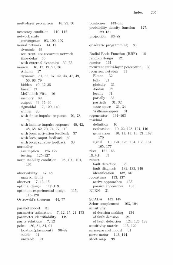
Index 205
multi-layer perceptron 16, 22, 30
necessary condition 110, 112network state
convergence 93, 100, 102neural network 14, 17
dynamic 49recurrent, see recurrent networktime-delay 30with external dynamics 30, 35
neuron 16, 17, 19, 21, 36Adaline 17dynamic 31, 36, 37, 42, 43, 47, 49,
50, 66, 79hidden 19, 32–35linear 71McCulloch-Pitts 16memory 39output 33, 35, 60sigmoidal 17, 129, 140winner 20with finite impulse response 70, 73,
74with infinite impulse response 40, 42,
48, 58, 62, 70, 74, 77, 119with local activation feedback 37with local ouput feedback 39with local synapse feedback 38
normalityassumption 125–127testing 125–127
norm stability condition 98, 100, 101,104
observability 47, 48matrix, 48, 49
observer 7, 13, 15optimal design 117–119optimum experimental design 115,
118–120Ostrowski’s theorem 44, 77
parallel model 31parameter estimation 7, 12, 15, 21, 173parameter identifiability 119parity relations 7, 12poles 80, 81, 84, 91
location(placement) 90–92stable 91unstable 91
positioner 143–145probability density function 127,
129–131projection 86–88
quadratic programming 83
Radial Basis Function (RBF) 18random design 121reactor 161recurrent multi-layer perceptron 33recurrent network 31
Elman 32fully 31globally 31Jordan 32locally 31parially 33partially 31, 32state-space 31, 34Williams-Zipser 31
regenerator 161–163residual
definition 10evaluation 10, 22, 123, 124, 140generation 10, 11, 13, 16, 21, 162,
179signal 10, 124, 126, 134, 135, 164,
165, 177riser 161–163RLMP 33robust
fault detection 123fault diagnosis 132, 133, 140identification 132, 137
robustness 133, 137active approaches 133passive approaches 133
RTRN 31
SCADA 142, 145Schur complement 103, 104sensitivity
of decision making 134of fault decision 126of fault detection 124, 126, 133
sensitivity matrix 115, 122series-parallel model 31servo-motor 143, 144short map 98

206 Index
significance level 130, 131, 135, 138,139
Simultaneous Perturbation StochasticApproximation, see SPSA
SPSA 55, 58, 61
gain sequences 56gradient estimate 56
outline 57
strong convergence 86
stability 78BIBO 77, 78
condition 97, 101, 104
margin 84, 92, 93
triangle 84stabilization 83, 88, 90, 93, 94
stable
model 79, 91
network 100region 91
solution 87
system 79, 81, 100, 107
stable system 107, 108statistical error bounds 132
sufficient condition 98, 105, 110
sugar evaporator 141
supportpoints 116
sequences 117SVD 107
tapped-delay lines 30temperature model 143, 149threshold 12, 124, 125, 130, 131
adaptive 123, 134, 135, 182constant 123, 136, 150, 170, 182fuzzy 135, 136nominal 136simple 124, 169, 182
true detection rate 26, 168, 170true isolation rate 26
uncertaintybands 138, 139region 138, 139
unit circle 79, 81, 91, 106, 107universal approximation theorem 68,
69unknown input observer 14unstable
model 79, 95system 80
vapour model 143, 148, 150, 151
winner takes all rule 20
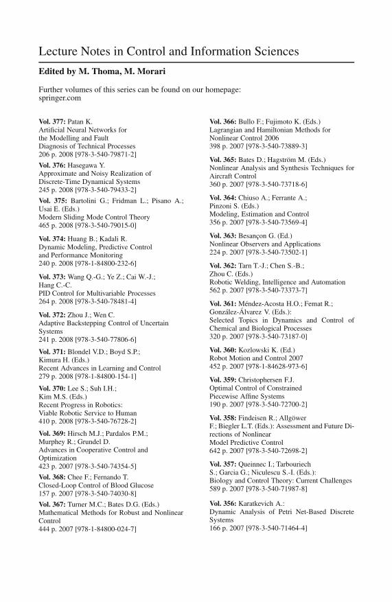
Lecture Notes in Control and Information Sciences
Edited by M. Thoma, M. Morari
Further volumes of this series can be found on our homepage:springer.com
Vol. 377: Patan K.Artificial Neural Networks forthe Modelling and FaultDiagnosis of Technical Processes206 p. 2008 [978-3-540-79871-2]
Vol. 376: Hasegawa Y.Approximate and Noisy Realization ofDiscrete-Time Dynamical Systems245 p. 2008 [978-3-540-79433-2]
Vol. 375: Bartolini G.; Fridman L.; Pisano A.;Usai E. (Eds.)Modern Sliding Mode Control Theory465 p. 2008 [978-3-540-79015-0]
Vol. 374: Huang B.; Kadali R.Dynamic Modeling, Predictive Controland Performance Monitoring240 p. 2008 [978-1-84800-232-6]
Vol. 373: Wang Q.-G.; Ye Z.; Cai W.-J.;Hang C.-C.PID Control for Multivariable Processes264 p. 2008 [978-3-540-78481-4]
Vol. 372: Zhou J.; Wen C.Adaptive Backstepping Control of UncertainSystems241 p. 2008 [978-3-540-77806-6]
Vol. 371: Blondel V.D.; Boyd S.P.;Kimura H. (Eds.)Recent Advances in Learning and Control279 p. 2008 [978-1-84800-154-1]
Vol. 370: Lee S.; Suh I.H.;Kim M.S. (Eds.)Recent Progress in Robotics:Viable Robotic Service to Human410 p. 2008 [978-3-540-76728-2]
Vol. 369: Hirsch M.J.; Pardalos P.M.;Murphey R.; Grundel D.Advances in Cooperative Control andOptimization423 p. 2007 [978-3-540-74354-5]
Vol. 368: Chee F.; Fernando T.Closed-Loop Control of Blood Glucose157 p. 2007 [978-3-540-74030-8]
Vol. 367: Turner M.C.; Bates D.G. (Eds.)Mathematical Methods for Robust and NonlinearControl444 p. 2007 [978-1-84800-024-7]
Vol. 366: Bullo F.; Fujimoto K. (Eds.)Lagrangian and Hamiltonian Methods forNonlinear Control 2006398 p. 2007 [978-3-540-73889-3]
Vol. 365: Bates D.; Hagström M. (Eds.)Nonlinear Analysis and Synthesis Techniques forAircraft Control360 p. 2007 [978-3-540-73718-6]
Vol. 364: Chiuso A.; Ferrante A.;Pinzoni S. (Eds.)Modeling, Estimation and Control356 p. 2007 [978-3-540-73569-4]
Vol. 363: Besançon G. (Ed.)Nonlinear Observers and Applications224 p. 2007 [978-3-540-73502-1]
Vol. 362: Tarn T.-J.; Chen S.-B.;Zhou C. (Eds.)Robotic Welding, Intelligence and Automation562 p. 2007 [978-3-540-73373-7]
Vol. 361: Méndez-Acosta H.O.; Femat R.;González-Álvarez V. (Eds.):Selected Topics in Dynamics and Control ofChemical and Biological Processes320 p. 2007 [978-3-540-73187-0]
Vol. 360: Kozlowski K. (Ed.)Robot Motion and Control 2007452 p. 2007 [978-1-84628-973-6]
Vol. 359: Christophersen F.J.Optimal Control of ConstrainedPiecewise Affine Systems190 p. 2007 [978-3-540-72700-2]
Vol. 358: Findeisen R.; AllgöwerF.; Biegler L.T. (Eds.): Assessment and Future Di-rections of NonlinearModel Predictive Control642 p. 2007 [978-3-540-72698-2]
Vol. 357: Queinnec I.; TarbouriechS.; Garcia G.; Niculescu S.-I. (Eds.):Biology and Control Theory: Current Challenges589 p. 2007 [978-3-540-71987-8]
Vol. 356: Karatkevich A.:Dynamic Analysis of Petri Net-Based DiscreteSystems166 p. 2007 [978-3-540-71464-4]

Vol. 355: Zhang H.; Xie L.:Control and Estimation of Systems withInput/Output Delays213 p. 2007 [978-3-540-71118-6]
Vol. 354: Witczak M.:Modelling and Estimation Strategies for FaultDiagnosis of Non-Linear Systems215 p. 2007 [978-3-540-71114-8]
Vol. 353: Bonivento C.; Isidori A.; Marconi L.;Rossi C. (Eds.)Advances in Control Theory and Applications305 p. 2007 [978-3-540-70700-4]
Vol. 352: Chiasson, J.; Loiseau, J.J. (Eds.)Applications of Time Delay Systems358 p. 2007 [978-3-540-49555-0]
Vol. 351: Lin, C.; Wang, Q.-G.; Lee, T.H., He, Y.LMI Approach to Analysis and Control ofTakagi-Sugeno Fuzzy Systems with Time Delay204 p. 2007 [978-3-540-49552-9]Vol. 350: Bandyopadhyay, B.; Manjunath, T.C.;Umapathy, M.Modeling, Control and Implementation of SmartStructures 250 p. 2007 [978-3-540-48393-9]
Vol. 349: Rogers, E.T.A.; Galkowski, K.;Owens, D.H.Control Systems Theoryand Applications for LinearRepetitive Processes482 p. 2007 [978-3-540-42663-9]
Vol. 347: Assawinchaichote, W.; Nguang, K.S.;Shi P.Fuzzy Control and Filter Designfor Uncertain Fuzzy Systems188 p. 2006 [978-3-540-37011-6]
Vol. 346: Tarbouriech, S.; Garcia, G.; Glattfelder,A.H. (Eds.)Advanced Strategies in Control Systemswith Input and Output Constraints480 p. 2006 [978-3-540-37009-3]
Vol. 345: Huang, D.-S.; Li, K.; Irwin, G.W. (Eds.)Intelligent Computing in Signal Processingand Pattern Recognition1179 p. 2006 [978-3-540-37257-8]
Vol. 344: Huang, D.-S.; Li, K.; Irwin, G.W. (Eds.)Intelligent Control and Automation1121 p. 2006 [978-3-540-37255-4]
Vol. 341: Commault, C.; Marchand, N. (Eds.)Positive Systems448 p. 2006 [978-3-540-34771-2]
Vol. 340: Diehl, M.; Mombaur, K. (Eds.)Fast Motions in Biomechanics and Robotics500 p. 2006 [978-3-540-36118-3]
Vol. 339: Alamir, M.Stabilization of Nonlinear Systems UsingReceding-horizon Control Schemes325 p. 2006 [978-1-84628-470-0]
Vol. 338: Tokarzewski, J.Finite Zeros in Discrete Time Control Systems325 p. 2006 [978-3-540-33464-4]
Vol. 337: Blom, H.; Lygeros, J. (Eds.)Stochastic Hybrid Systems395 p. 2006 [978-3-540-33466-8]
Vol. 336: Pettersen, K.Y.; Gravdahl, J.T.;Nijmeijer, H. (Eds.)Group Coordination and Cooperative Control310 p. 2006 [978-3-540-33468-2]
Vol. 335: Kozłowski, K. (Ed.)Robot Motion and Control424 p. 2006 [978-1-84628-404-5]
Vol. 334: Edwards, C.; Fossas Colet, E.;Fridman, L. (Eds.)Advances in Variable Structure and Sliding ModeControl504 p. 2006 [978-3-540-32800-1]Vol. 333: Banavar, R.N.; Sankaranarayanan, V.Switched Finite Time Control of a Class ofUnderactuated Systems99 p. 2006 [978-3-540-32799-8]
Vol. 332: Xu, S.; Lam, J.Robust Control and Filtering of Singular Systems234 p. 2006 [978-3-540-32797-4]
Vol. 331: Antsaklis, P.J.; Tabuada, P. (Eds.)Networked Embedded Sensing and Control367 p. 2006 [978-3-540-32794-3]
Vol. 330: Koumoutsakos, P.; Mezic, I. (Eds.)Control of Fluid Flow200 p. 2006 [978-3-540-25140-8]
Vol. 329: Francis, B.A.; Smith, M.C.; Willems,J.C. (Eds.)Control of Uncertain Systems: Modelling,Approximation, and Design429 p. 2006 [978-3-540-31754-8]
Vol. 328: Loría, A.; Lamnabhi-Lagarrigue, F.;Panteley, E. (Eds.)Advanced Topics in Control Systems Theory305 p. 2006 [978-1-84628-313-0]
Vol. 327: Fournier, J.-D.; Grimm, J.; Leblond, J.;Partington, J.R. (Eds.)Harmonic Analysis and Rational Approximation301 p. 2006 [978-3-540-30922-2]
Vol. 326: Wang, H.-S.; Yung, C.-F.; Chang, F.-R.H∞ Control for Nonlinear Descriptor Systems164 p. 2006 [978-1-84628-289-8]


