63
Volume No.4 December, 2013 Asia-Pacific GAW Greenhouse Gases News letter ISSN 2093-9590 11-1360000-000970-10
Volume No.4December, 2013
Asia-Pacific GAW Greenhouse Gases
Newsletter
ISSN 2093-9590
11-1360000-000970-10

Published by KMA in Dec. 2013.
Asia-Pacific GAW Greenhouse Gases NewsletterVolume No.4 December, 2013


CONTENTS
∙ Atmospheric Methane Characteristics in AMY, Korea, 2012 ························· 1
∙ NOAA Measurements of Long-lived Greenhouse Gases ································ 6
∙ Ground-based monitoring of greenhouse gases (CO2, CH4) along the west coast of India: Role of Indian summer monsoon ············································ 10
∙ Establishment of Continuous Greenhouse Gas Observation Capacity in Northern Vietnam through a Swiss-Vietnamese Collaboration ····················· 16
∙ Preliminary Results of Greenhouse Gases Observed at Lulin Atmospheric Background Station (LABS), Taiwan ···························································· 22
∙ Development of Southeast Asia-Australian Atmospheric Observation Capacity ·· 26
∙ Forty Years of Baseline CO2 Measurements at Baring Head, New Zealand ····· 30
∙ The Greenhouse Gases Observation and Analysis at GAW stations in Malaysia ········································································································· 35
∙ Gravimetric standards of Greenhouse gases at ambient levels ······················ 41
∙ Intercomparison experiments for Greenhouse Gases Observation (iceGGO) in Japan ··········································································································· 45
∙ Current Activities of World Calibration Center of SF6 ·································· 50

Asia-Pacific GAW Greenhouse Gases Newsletter Volume No. 4, 2013 1
Atmospheric Methane Characteristics in AMY, Korea, 2012
Haeyoung Lee and Bok-Haeng Heo Korea Global Atmosphere Watch Center
Korea Meteorological Administration
The Fifth Assessment Report (AR5) of the United Nations Intergovernmental Panel on Climate
Change (IPCC) published in September 2013 reported that there is a clear human influence on the ongoing global warming. In addition, atmospheric concentrations of carbon dioxide, methane, and nitrous oxide have increased to unprecedented levels in at least the last 800,000 years.
Especially, even though methane is the most important greenhouse gas next to carbon dioxide, the relative contributions to various processes that produce methane are uncertain while the sink is quite well understood indicating it arises primarily from the activity of hydroxyl radical which is involved in photochemical oxidation reaction.
Asia regions are well known for the main source of methane due to rice paddies, plateaus during monsoon, and tropical wetlands [1], [2], [3], [4]. For Korea, methane is released mainly from agriculture (40% methane emissions in total) and energy sector (30%) [5]. In Korea, methane studies are focusing on only emission source interestingly. However, atmospheric methane studies are very important to understand the growth rate because they reflect the global methane budgets which delicately balance large sink and sources at present.
The Korean Peninsula is not only located in downwind area from Asia continents due to westerly wind, but also affected by seasonal flow patterns indicating the main wind stream is southwesterly in spring, southerly in summer, easterly in autumn, and northwesterly in winter, respectively. Especially, Anmyeondo (AMY) is in western part of the Korean Peninsula and one of GAW (Global Atmosphere Watch) regional stations that AMY could monitor the methane not only from local area, but also from other Asia continents. In here, the evidence is presented from atmospheric trajectories that explain some of synoptic and seasonal scale variability in methane by relating it to flow patterns and locations of source and sink in AMY.
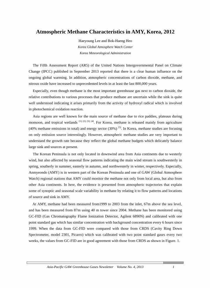
At AMY, methane had been measured from1999 to 2003 from the inlet, 67m above the sea level, and has been measured from 87m using 40 m tower since 2004. Methane has been monitored using GC-FID (Gas Chromatography Flame Ionization Detector, Agilent 6890N) and calibrated with one point standard gas which has similar concentration with background concentration every 6 hours since 1999. When the data from GC-FID were compared with those from CRDS (Cavity Ring Down Spectrometer, model 2301, Picarro) which was calibrated with two point standard gases every two weeks, the values from GC-FID are in good agreement with those from CRDS as shown in Figure. 1.
2 Asia-Pacific GAW Greenhouse Gases Newsletter Volume No. 4, 2013
Figure 1. Temporal variation of hourly mean of methane measured by GC-FID (red spots) and CRDS (black spots) in 2012, AMY, Korea (left) and the scatter plot of CRDS and GC-FID using hourly mean concentrations (right).
The seasonal mean concentrations of methane were high in the order of autumn>winter> summer>spring (Table 1.). Methane shows the lowest concentration in summer due to the OH radical and high mixing height generally. However, mean concentration of methane in summer at AMY was higher than that of spring, similar with winter’s and its standard deviation was the highest indicating maximum concentration was the highest (2551 ppb) and the minimum concentration was the lowest (1773 ppb).
Table 1. The results of methane measured with GC-FID at AMY in 2012
Conc.(ppb) Spring (MAM) Summer (JJA) Autumn (SON) Winter (DJF)
Mean 1937 1953 1961 1954
Std. 37 116 67 43
Median 1927 1926 1940 1941
Maximum 2138 2551 2407 2179
Minimum 1836 1773 1826 1792
N 1675 2172 2183 2161
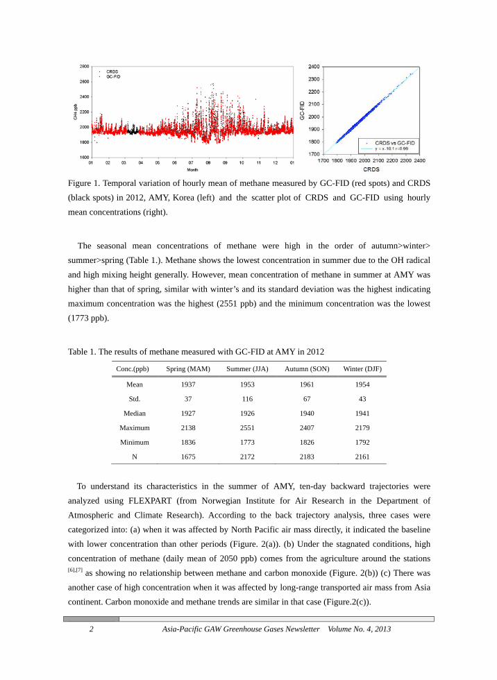
To understand its characteristics in the summer of AMY, ten-day backward trajectories were
analyzed using FLEXPART (from Norwegian Institute for Air Research in the Department of Atmospheric and Climate Research). According to the back trajectory analysis, three cases were categorized into: (a) when it was affected by North Pacific air mass directly, it indicated the baseline with lower concentration than other periods (Figure. 2(a)). (b) Under the stagnated conditions, high concentration of methane (daily mean of 2050 ppb) comes from the agriculture around the stations [6],[7] as showing no relationship between methane and carbon monoxide (Figure. 2(b)) (c) There was another case of high concentration when it was affected by long-range transported air mass from Asia continent. Carbon monoxide and methane trends are similar in that case (Figure.2(c)).
Asia-Pacific GAW Greenhouse Gases Newsletter Volume No. 4, 2013 3
(a)
(b)
(c)
Figure 2. The ten-day backward trajectory of FLEXPART (left column) and CO and CH4 concentrations from GC-FID and CRDS respectively (right column) in (a) the low concentration case, (b) the high concentration case under the stagnated condition and (c) the high concentration case due to long-range transported air mass from the Asia continent during summer period, 2012, AMY.
4 Asia-Pacific GAW Greenhouse Gases Newsletter Volume No. 4, 2013
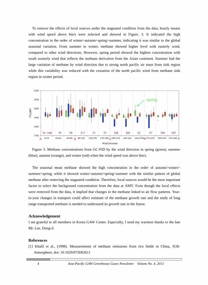
To remove the effects of local sources under the stagnated condition from the data, hourly means with wind speed above 6m/s were selected and showed in Figure. 3. It indicated the high concentration in the order of winter>autumn>spring>summer, indicating it was similar to the global seasonal variation. From summer to winter, methane showed higher level with easterly wind, compared to other wind directions. However, spring period showed the highest concentration with south westerly wind that reflects the methane derivation from the Asian continent. Summer had the large variation of methane by wind direction due to strong north pacific air mass from sink region while this variability was reduced with the cessation of the north pacific wind from methane sink region in winter period.
Figure 3. Methane concentrations from GC-FID by the wind direction in spring (green), summer
(blue), autumn (orange), and winter (red) when the wind speed was above 6m/s.
The seasonal mean methane showed the high concentration in the order of autumn>winter>
summer>spring, while it showed winter>autumn>spring>summer with the similar pattern of global methane after removing the stagnated condition. Therefore, local sources would be the most important factor to select the background concentration from the data at AMY. Even though the local effects were removed from the data, it implied that changes in the methane linked to air flow patterns. Year-to-year changes in transport could affect estimate of the methane growth rate and the study of long range transported methane is needed to understand its growth rate in the future.
Acknowledgement I am grateful to all members in Korea GAW Center. Especially, I send my warmest thanks to the late Mr. Lee, Dong-il.
References [1] Khalil et al., (1998). Measurements of methane emissions from rice fields in China, JGR-
Atmosphere, doi: 10.1029/97JD02611
Asia-Pacific GAW Greenhouse Gases Newsletter Volume No. 4, 2013 5
[2] Ye, D. Z. and Wu, G. X. (1998). The role of the heat sources of the tibetan plateau in the general circulation, Meteo. Atmos. Phys., 67, 181-198, 1998.
[3] Huang, Y., et al., (2004) Modeling methane emission from rice paddies with varios agricultural practices, J. Geophys. Res.-Atmos., 109, D08113, doi: 10.1029/2003JD004401.
[4] Dlugokencky E. J. et al (2009). Observational constraints on recent increases in the atmosphere CH4 burden, Geophysical Research letters, 36, doi: 10.1029/2009GL039780
[5] National Greenhouse Gas Inventory Report of Korea, 2012 [6] Dlugokencky E. J. et al (1993) The relationship between the methane seasonal cycle and regional
sources and sinks at Tae-ahn Peninsula, Korea, Atmo. Environ. 27(14) [7] Yang et al., (1999). Diurnal variation of methane emission from paddy fields at different growth
stages of rice cultivation in Taiwan, Agric., Ecosyst. & Environ. 76(23)
6 Asia-Pacific GAW Greenhouse Gases Newsletter Volume No. 4, 2013
NOAA Measurements of Long-lived Greenhouse Gases
Edward J. Dlugokencky1, Andrew Crotwell1,2, Ken Masarie1, James White3, Patricia Lang1,
and Molly Crotwell1,2
1. National Oceanic and Atmospheric Administration, Earth System Research Laboratory, Global Monitoring
Division, Boulder, Colorado, USA, 2. CIRES, Univ. of Colorado, Boulder, CO, USA, 3. INSTAAR, Univ. of
Colorado, Boulder, CO, USA
Introduction
NOAA Earth System Research Laboratory, Global Monitoring Division, Carbon Cycle Group (CCG) began monitoring CO2 from discrete flask samples in the late-1960s, and has since added measurements of other important long-lived greenhouse gases and related tracers, including isotopes through collaboration with the University of Colorado, INSTAAR, from these flasks. Our group also has programs to measure CO2 and CH4 continuously at NOAA’s background observatories, measure CO2 and other tracers from tall towers, and measure long-lived greenhouse gases (LLGHG) from discrete samples collected on light aircraft. Our group, in collaboration with another group in our division, has also developed a standards program that provides SI-traceable standards to our NOAA programs and the WMO GAW community. Here some key results from CCG’s global cooperative air sampling network are given for CO2, CH4, N2O, and SF6.
Sampling and analysis methods
Air sample pairs are collected approximately weekly in 2.5 L flasks from ~60 sites (as of 2013) in NOAA’s global cooperative air sampling network [1] (also http://www.esrl.noaa.gov/gmd/ccgg/flask. html). Flasks are flushed and pressurized to ~1.2 atm with a portable sampler. Samples are collected under conditions when air is representative of large, well-mixed volumes of the atmosphere to facilitate comparison with simulations from chemical transport models that have relatively large grid-scale resolution. Analytical methods are as follows: CO2: NDIR; CH4: GC/FID; N2O/SF6: GC/ECD. All instrument responses are calibrated with standards on the respective WMO GAW mole fraction scales maintained at NOAA and reported as dry-air mole fractions (CO2 and CH4 data path: ftp://aftp.cmdl.noaa.gov/data/trace_gases/<co2 or ch4>/flask/surface/). To calculate means representative of large spatial scales, data from a subset of globally-distributed remote boundary layer sites were fitted with curves to smooth variability with periods less than ~40 days [1]. Synchronized points were extracted from these curves at approximately weekly intervals and smoothed as a function of latitude to define an evenly spaced matrix of surface LLGHG mole fractions as a function of time and latitude. This matrix was used to calculate global and zonal averages.
Asia-Pacific GAW Greenhouse Gases Newsletter Volume No. 4, 2013 7
Results
CO2: Since 1750, ~385 billion tons of carbon has been emitted into the atmosphere as CO2 by combustion of fossil fuels and production of cement. About half of these emissions have occurred since the mid-1970s [2]. This carbon is partitioned into three mobile reservoirs: atmosphere, oceans, and terrestrial biosphere. Atmospheric CO2 has increased from about 278 ppm (ppm=μmol mol-1) at the start of the industrial revolution to more than 390 ppm today. The atmospheric increase contributes ~1.85 W m-2 of radiative forcing (see e.g., http://www.esrl.noaa.gov/gmd/aggi/). CO2 that enters the ocean increases the acidity (decreased pH) of surface waters through carbonate chemistry. This can have detrimental effects on organisms that contain calcium carbonate, for example the shells of plankton near the bottom of the ocean food chain and corals. Increasing acidity will cause calcium carbonate to dissolve, destroying these creatures.
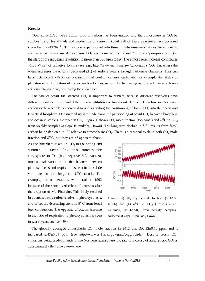
The fate of fossil fuel derived CO2 is important to climate, because different reservoirs have different residence times and different susceptibilities to human interference. Therefore much current carbon cycle research is dedicated to understanding the partitioning of fossil CO2 into the ocean and terrestrial biosphere. One method used to understand the partitioning of fossil CO2 between biosphere and ocean is stable C isotopes in CO2. Figure 1 shows CO2 mole fraction (top panel) and δ13C in CO2 from weekly samples at Cape Kumukahi, Hawaii. The long-term decline in δ13C results from fossil carbon being depleted in 13C relative to atmospheric CO2. There is a seasonal cycle in both CO2 mole fraction and δ13C, but they are of opposite phase. As the biosphere takes up CO2 in the spring and summer, it favors 12C; this enriches the atmosphere in 13C (less negative δ13C values). Inter-annual variation in the balance between photosynthesis and respiration is seen in the subtle variations in the long-term δ13C trends. For example, air temperatures were cool in 1992 because of the short-lived effect of aerosols after the eruption of Mt. Pinatubo. This likely resulted in decreased respiration relative to photosynthesis, and offset the decreasing trend in δ13C from fossil fuel combustion. The opposite effect, an increase in the ratio of respiration to photosynthesis is seen in warm years such as 1998.
The globally averaged atmospheric CO2 mole fraction in 2012 was 392.52±0.10 ppm, and it increased 2.43±0.09 ppm (see http://www.esrl.noaa.gov/gmd/ccgg/trends/). Despite fossil CO2 emissions being predominantly in the Northern hemisphere, the rate of increase of atmospheric CO2 is approximately the same everywhere.
Figure 1.(a) CO2 dry air mole fractions (NOAA
ESRL) and (b) δ13C in CO2 (University of
Colorado, INSTAAR) from weekly samples
collected at Cape Kumukahi, Hawaii.

8 Asia-Pacific GAW Greenhouse Gases Newsletter Volume No. 4, 2013
CH4: The contribution of CH4 to anthropogenic radiative forcing, including direct and indirect effects, is about 0.7 W m-2. While ~2/3 of its emissions are from anthropogenic sources, natural emissions of CH4, predominantly from wetlands, are a potential strong climate feedback because emission rates depend strongly on temperature and precipitation. In the Arctic, where surface temperatures are increasing at twice the global rate, there is the potential for increases in CH4 emissions from wetlands. The Arctic also contains large stores of organic carbon in permafrost and in hydrates, but increases in emissions from these climate-sensitive sources have not yet been detected in atmospheric observations. Anthropogenic sources such as biomass burning are also susceptible to changing climate through changes in precipitation. Dry conditions during the strong El Niño of 1997 and 1998 resulted in an estimated 50% increase in CH4 emissions from biomass burning in the tropics and high northern latitudes relative to normal [3].
After a decade of near-zero growth, atmospheric CH4 began increasing again globally in 2007 [4], [5], as shown in Figure 1. The increase was driven by increased Arctic and tropical emissions. CO measurements in the same air samples indicate little contribution from enhanced biomass burning since 2007. Likely drivers for increased emissions in 2007 are anomalously high temperatures and precipitation in wetland regions, particularly in the Arctic. Since 2007, atmospheric CH4 continues to increase at ~6 ppb yr-1. Despite continued warmth in the Arctic, emissions there returned to normal levels in 2008. The causes of the continued global increase are not clear, but greater than average precipitation in tropical wetland regions and increased anthropogenic emissions are likely the largest contributors. Unfortunately, the current atmospheric CH4 observing network is not sufficient to determine with certainty the causes of the CH4 increase since 2007.
N2O: Nitrous oxide contributes the third-most radiative forcing by LLGHGs since 1750, and its stratospheric ozone depletion potential-weighted emissions are now largest of all ozone depleting substances. Based on long-term continuous measurements at NOAA observatories, it has increased at ~0.78 ppb yr-1 for more than 30 years (http://www.esrl.noaa.gov/gmd/hats/combined/N2O.html). Because N2O has a long lifetime (~130 yr) and its emission rates are small, spatial gradients are small. This, in turn, requires a relatively high degree of internal consistency across measurement networks, if the observations are going to be used with a chemical transport model to calculate emissions at regional to continental scales. CCG has been measuring N2O in discrete air samples since mid-1997. Despite poorer repeatability of the CCG N2O measurements from flasks than from in situ analyzers, the greater spatial coverage of the CCG measurements has helped improve knowledge of the large
Figure 2. (a) Solid line shows globally
averaged CH4 dry air mole fractions; dashed
line is a deseasonalized trend curve fitted to the
global averages. (b) Instantaneous growth rate
for globally averaged atmospheric CH4 (solid
line; dashed lines are uncertainties at 68%
confidence limit).

Asia-Pacific GAW Greenhouse Gases Newsletter Volume No. 4, 2013 9
scale distribution of emissions [6]. In future, isotopic measurements of N2O from CCG discrete samples may further improve our knowledge of the global N2O budget.
SF6: Sulfur hexafluoride is emitted almost entirely from anthropogenic processes. Because its lifetime is extremely long (~3200 yr) and it is well-mixed in the atmosphere, observations from relatively few sites can be used to estimate total global emissions. Such estimates show that emissions reported to the UNFCCC by Annex I countries are substantially underestimated [7]. As with N2O, CCG measurements are useful in understanding the spatial patterns of SF6 emissions. Additionally, the observations have been used to test transport in atmospheric chemical transport models. For example, Peters et al. [8] used CCG SF6 measurements to show that the commonly used model “TM5” overestimates the latitudinal gradient of SF6 by 19% and that mixing within the planetary boundary layer in the model is too slow.
References
[1] Dlugokencky, EJ et al. (1994), The growth rate and distribution of atmospheric methane, J. Geophys. Res., 99(D8), 17021–17043, doi:10.1029/94JD01245.
[2] Marland, G et al. (2008), Global, Regional, and National CO2 Emissions. In Trends: A Compendium of Data on Global Change. Carbon Dioxide Information Analysis Center, Oak Ridge National Laboratory, U.S. Department of Energy, Oak Ridge, Tenn., U.S.A.
[3] van der Werf, GR et al. (2006), Interannual variability in global biomass burning emissions from 1997 to 2004, Atmospheric Chemistry and Physics, 6, 3423-3441.
[4] Rigby, M et al. (2008), Renewed growth of atmospheric methane, Geophys. Res. Lett., 35, L22805, doi:10.1029/2008GL036037.
[5] Dlugokencky, EJ et al. (2009), Observational constraints on recent increases in the atmospheric CH4 burden, Geophys. Res. Lett., 36, L18803, doi:10.1029/2009GL039780.
[6] Hirsch, AI et al. (2006) Inverse modeling estimates of the global nitrous oxide surface flux from 1998-2001, Global Biogeochemical Cycles, 20, doi:10.1029/2004GB002443.
[7] Levin, I et al. (2010), The global SF6 source inferred from long-term high precision atmospheric measurements and its comparison with emission inventories, Atmos. Chem. Phys., 10(6), 2655–2662, doi:10.5194/acp- 10-2655-2010.
[8] Peters, W et al. (2004), Toward regional-scale modeling using the two-way nested global model TM5: Characterization of transport using SF6, J. Geophys. Res., 109, D19314, doi:10.1029/ 2004JD005020.

10 Asia-Pacific GAW Greenhouse Gases Newsletter Volume No. 4, 2013
Ground-based monitoring of greenhouse gases (CO2, CH4) along
the west coast of India: Role of Indian summer monsoon
Yogesh K. Tiwari1, Ramesh Vellore1, K. Ravi Kumar1, and Marcel V. van der Schoot2 1Centre for Climate Change Research, Indian Institute of Tropical Meteorology, Pune, India
2CSIRO Marine and Atmospheric Research, Aspendale, Australia
The paucity of ground-based greenhouse gas (GHG) monitoring over the Indian subcontinent has been posing a stringent limitation to the estimates of CO2 sources and sinks. According to a recent report published by the Ministry of Environment and Forests (MoEF), Government of India (http://moef.nic.in/downloads/public-information/Report_INCCA.pdf), the total GHG emissions in India have substantially increased from 1252 to 1905 million tons during 1994-2007 at an annual growth rate of 3.3%. With limited ground-based observational resources, it was seen that some sectors such as the cement production, electricity generation, and transport have provided greater contribution to this significant growth by 6%, 5.6%, and 4.5% respectively during this time. Estimates of total fossil-fuel CO2 emissions from Indian subcontinent are: 189 TgC in 1990, 324 TgC in 2000, 385 TgC in 2005 and 508 TgC in 2009 with an increasing rate of about 7% per year during the past decade[1] [source: Carbon Dioxide Information Analysis Center (CDIAC), USA]. One of intriguing sink factors is that some of the GHG emissions are likely to be compensated by vegetation uptake over the Indian subcontinent[2],[3] which still remains an unresolved issue that warrants immediate attention. In response to land-sea thermal contrast, the largest volume of precipitation over the subcontinent is observed during the monsoon months [June through September (JJAS) in summer and December through February (DJF) in winter[4], [5], [6]. As the southwesterly moist-laden winds during the Indian summer monsoon initially arrives at the west coast of India and then spreads over the subcontinent, the maritime transport mechanisms are imperative for accurate source region estimates. The influence of the continental air mass transport during DJF due to seasonal wind reversal is also equally important. More importantly, the GHG residence times over the oceanic and continental regions during their transport are of great importance. Therefore, the transport mechanisms associated with the monsoon meteorology in the vicinity of the complex mountainous regions constitutes the focal point of this study to understand the role of GHG transport and sinks in the west coast of Indian subcontinent using observational and modeling resources. Currently, there are two operational stations along the west coast of India, one at Cape Rama (CRI), Goa (15.08° N, 73.83° E, elevation =50 m asl) (Fig. 1) that has a long observational record for more than a decade. The CO2 seasonal behavior at CRI has clear signals driven by monsoon meteorology and terrestrial ecosystem variability[7], [8].Another GHG monitoring site located over the Western Ghats mountains is Sinhagad (SNG; 200 km from the Arabian sea; 73.75o E, 18.35o N, elevation = 1600 m asl) which is operational since 2010 that concatenates the CO2 routine monitoring along the west coast of India (Fig. 1)[9].Similar to the features observed at CRI, SNG also consistently indicates

the seasinfluencDJF. Seassociatesurface-bobservatshed moparticulaobservat
(NDVI),[15] and obtainedrainfall gthe highin Octob(June) m
Asia-Pac
sonal changced by maritieveral recened with GHbased, but mtions or fromore insight ar, is aimed tions at CRI
Figure
Figure 2 sho, and rainfallrainfall [16],
d from NOAgauges locat
hest possible ber both at SNmonth.
cific GAW Gre
es of CO2 ime air massnt observatioGs and the
mostly restrim the modelto the undeat demonst
and SNG.
1.Observatio
ows the monl (mm) durin
17] datasets A/AVHRR aed over Indiadensity of gNG and CRI
eenhouse Gase
to reversal es during JJAonal and mIndian summ
icted to midl simulationserstanding otrating the i
ons sites Cap
nthly climatong 2000-2010
archived atas well as froa. Zero ND
green leaves. I. Indian sum
es Newsletter
of wind paAS, while inodeling studmer monsoo-to-upper tros. The surfac
of the variabinfluence of
pe Rama (CR
ological mean0 valid over t 1° × 1° rom MODIS/ADVI means n
NDVI showmmer monsoo
Volume No.
atterns. Thenfluenced by dies have en [10], [11], [12].oposphere Cce-based obbility and sef the Indian
RI) and Sinha
n of Normalithe site locat
resolution arAQUA. The
no vegetationws minimum on rainfall at
. 4, 2013
se two sitesthe continen
elicited the . However, t
CO2 obtainedservations ateasonal chansummer mo
agad (SNG) o
ized Differentions at SNGre used in te rainfall datan and as high
during Aprit CRI (SNG)
s are predontal air massegeneral conthese studies
d either fromt CRI and Snges. This sonsoon on t
over India.
nce VegetatiG and CRI. Nthis study. Naset is based
h as 0.8 - 0.9 l-May and m) is maximum
11
minantly es during nnections s are not
m aircraft SNG will study, in the GHG
on Index NDVI [14],
NDVI is d on 1803
indicates maximum m in May

12
Figure 2Sinhaga
FigureHawaii, 2012 areSNG obduring ssignaturthan in m
FigureMLO as4.68 E, CO2 andmean ofentire ye
The omonsoondebatablon the rsinks frowell as waccuratecarbon c
2.NDVI (lefd (SNG) mo
e 3 shows a USA agains
e used for cobservations ssummer (winres of CO2 dumarine windse 4 compares well as at
94 m asl )d CH4 concenf CH4 concenear which imobservationsn circulationle strengthenegional climom the neighwith the aid
e regional idcycle over th
Asia-P
ft panel) andonitoring site
comparisonst the values omparison wshow strongenter) monsoouring summes, s climatologt Seychelles () from the sontrations indintrations obse
mplicates that clearly ind
n along the ning and wea
mate assessmehboring regioof full suite entification
he Indian sub
Pacific GAW G
d Rainfall (s.
n of daily meat CRI and
with CRI ander trend andon months [1
er monsoon
gical mean of(SEY;4.67 Southern hemicate lower verved at SEYt these two sidicate that gwest coast o
akening of ment over Indons. In lieu ochemistry trof CO2 and continent.
Greenhouse G
right panel)
ean atmosphSNG. MLOd 2010-2013d seasonality18]. In accordmonths as C
f CO2 and CHS, 55.17 E, isphere. Durvalues than oY and CGO gites are primgreenhouse gof India. In
monsoonal flodia [13] owingof this, a detransport modother tracer
Gases Newslett
climatology
heric CO2 obO daily mean with SNG.
y. Marine (cdance to this
CO2 signature
H4 concentra7m asl) and
ring summerobserved at generally indarily dominagas transporthe advent
ows, the carbg to strong detailed furtherdels are indisspecies for
ter Volume N
y at the Cap
servations atn CO2 obserAs compare
ontinental) ws, CRI and Ses are richer
ations observd Cape Grimr monsoon mMLO (Fig.4
dicate smoothated by the mrt is stronglyof changing
bon cycle hasependence or analysis of spensable at better under
No. 4, 2013
pe Rama (C
t Mauna Loarvations durined to MLO, winds dominSNG indicatin continent
ved at CRI, Sm (CGO; 40.6months CRI 4a, b). Climah variation d
marine signaty influenced climate eras serious impf carbon sou
f CO2 observthis time tow
rstanding of
CRI) and
a (MLO) ng 2009-CRI and
nate CRI ed lower tal winds
SNG, and 68 S, 14observed
atological during the ures. d by the a and the plications urces and vations as wards an
f regional
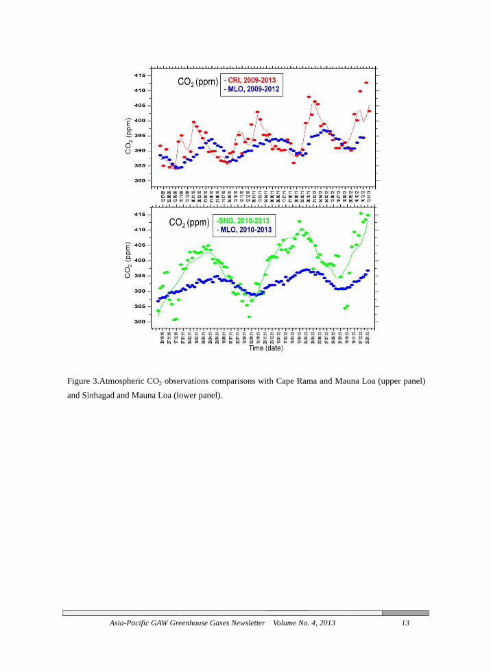
Figure 3and Sinh
Asia-Pac
3.Atmospherhagad and M
cific GAW Gre
ric CO2 obserMauna Loa (lo
eenhouse Gase
rvations comower panel).
es Newsletter
mparisons wi
Volume No.
ith Cape Ram
. 4, 2013
ma and Maun
na Loa (upp
13
er panel)

14
Figure 4Mauna LSinhaga
Referen[1] Bod
EmisDepaonlin
[2] Lal,Mon
[3] Patrabalan4163
[4] GosIncre
4.ComparisoLoa (b) CH4 d, Seychelle
nces en, T. A., Mssions, Carbartment of Ene at: http://c, M., Singhnitoring and Aa PK, Niwa Ynce of South3−4175. swami B.N.,easing trend
Asia-P
n of climatoobservation
s (SEY) and
Marland, G., bon Dioxide Energy, Oakcdiac.ornl.goh, R., 2000.Assessment 6Y, Schuck TJh Asia constr
,Venugopal d of Extreme
Pacific GAW G
ological means at Cape Ra
Cape Grim
and AndresInformation
k Ridge, Tenov/trends/emi Carbon se60 (3), 315-3J, Brenninkmrained by pas
V., Sengupte Rain Even
Greenhouse G
an of atmospama and Mau(CGO).
. R. J.: Globn Analysis Cnn., USA, dis/tre glob.ht
equestration 327. meijer CAM, ssenger aircr
ta D., Madhnts over Indi
Gases Newslett
pheric (a) COuna Loa (c)
bal, RegionaCenter, Oak doi:10.3334/Ctml, last accepotential of
Machida T, raft CO2 mea
husoodanan ia in a Warm
ter Volume N
O2 observatiCH4 observa
al, and NatioRidge Natio
CDIAC/0000ess: 19 May 2f Indian for
Matsueda Hasurements. A
M.S., Xaviming Enviro
No. 4, 2013
ions Cape Rations at Cap
onal Fossil-Fonal Labora01 V2010, 2011, 2009. rests. Enviro
H, et.al., 2011AtmosChem
er Prince Konment,Scien
Rama and pe Rama,
Fuel CO2 atory, US available
onmental
1. Carbon mPhys 11:
K., 2006: nce, 314,
(a)
(b
(c
)
b)
c)
Asia-Pacific GAW Greenhouse Gases Newsletter Volume No. 4, 2013 15
5804, 1 December, 1442-1445. [5] Wang, Y.J et al 2006. Interhemispheric anti-phasing of rainfall during the last glacial period,
Quart.Sci, Rev., 25, 3391-3403. [6] Webster PJ, Magana VO, Palmer TN, Shukla J, Tomas RA, Yanai M, Yasunari T. 1998. Monsoons:
processes, predictability, and the prospects for prediction. Journal of Geophysical Research 103: 14 451–14 510.
[7] Bhattacharya, S.K., Borole, D.V., Francey, R.J., Allison, C.E., Steele, L.P., Krummel, P.B., Langenfelds, R.L., Masarie, K.A., Tiwari, Y.K., Patra, P.K., 2009. Trace gases and CO2 isotope records from Cabo de Rama, India. Current Science 97, 1336e1344.
[8] Tiwari YK, Patra PK, Chevallier F, Francey RJ, Krummel PB, Allison CE, et. al. CO bservations at Cape Rama, India for the period of 1993-2002: implications for onstraining Indian emissions. CurrSci 101: 1562−1568, 2011.
[9] Yogesh K. Tiwari, K. Ravi Kumar, 2012, GHG observation programs in India, Asian GAW greenhouse gases news letter, Vol.3, ISSN2093-9590, Dec.2012, Korea Meteorological Administration, South Korea, December 2012.
[10] Schuck, T. J., Brenninkmeijer, C. a. M., Baker, a. K., Slemr, F., Velthoven, P. F. J. V., Zahn, A., 2010, Greenhouse gas relationships in the Indian summer monsoon plume measured by the CARIBIC passenger aircraft, Atmos. Chem. Phys., 10, 3965-3984, 2010
[11] Chadwick R., Good P., Andrews T., Martin G., 2013, Surface Warming Patterns Drive Tropical Rainfall Pattern Responses to CO 2 Forcing on All Timescales, Geophysical Research Letters (accepted article)
[12] Polson D., Hegerl G. C., Allan R. P., Sarojini B. Balan, 2013, Have greenhouse gases intensified the contrast between wet and dry regions? Geophysical Research Letters, vol.50, Aug.2013
[13] Cherchi, A., Alessandri, A., Masina, S., Navarra, A., 2010. Effects of increased CO2 levels on monsoons. Climate Dynamics. http://dx.doi.org/10.1007/s00382-010-0801-7.
[14] Leeuwen, V., Wim, J.D., Huete, A.R., Laing, W.L., 1999. MODIS vegetation index compositing approach: a prototype with AVHRR data, Remote Sensing of Environment 69, 264-280.
[15] Huete, A., Didan, K., Miura, T., Rodriguez, E.P., Gao, X., Ferreira, L.G., 2002. Overview of the radiometric and biophysical performance of the MODIS vegetation indices, Remote Sensing of Environment 83, 195- 213.
[16] Rajeevan, M., Bhate, J., Kale, J.D., Lal, B., 2005. Development of a high resolution daily gridded rainfall data for the Indian region. India Meteorological Department Met Monograph Climatology 22, 27.
[17] Rajeevan, M., Bhate, J., Kale, J.D., Lal, B., 2006. High resolution daily gridded rainfall data for the Indian region: analysis of break and active monsoon spells. Current Science, 91, 296-306.
[18] Yogesh K. Tiwari,J.V. Revadekar, K. Ravi Kumar., 2013. Variations in atmospheric Carbon Dioxide and its association with rainfall and vegetation over India, Atmospheric Environment, Volume 68, April 2013, Pages 45–51, http://dx.doi.org/10.1016/j.atmosenv.2012.11.040.
16 Asia-Pacific GAW Greenhouse Gases Newsletter Volume No. 4, 2013
Establishment of Continuous Greenhouse Gas Observation Capacity in Northern Vietnam through a Swiss-Vietnamese Collaboration
Duong Hoang Long
National Hydro-Meteorological Service,
Science-Technology and International Cooperation Dept., Hanoi, Vietnam
I. Introduction
The project Capacity Building and Twinning for Climate Observing Systems (CATCOS) [1]that will last from mid-2011 to 2013. The project is supported by the Swiss Agency for Development and Cooperation (SDC) with the Federal Office of Meteorology and Climatory MeteoSwiss as the coordinating partner on the part of Switzerland. The project addresses the need to improve climate observations world-wide, but particularly in developing countries and countries in transition. The Project focuses on atmospheric observations and will be implemented by the Paul Scherrer Institute (PSI, for the aerosol part), and by the Swiss Laboratories for Materials Testing and Research (EMPA, for the atmospheric trace gas part).
The International partners and beneficiaries of this project are countries in South America, in Africa, and in Asia. These are represented by the Bureau of Meteorology, Climatory and Geophysics (MMKG, Indonesia), the Dirección Meteorológica de Chile (DMC, Chile), the Kenya Meteorological Department (KMD, Kenya), and the National Hydro-Meteorological Service (NHMS, Vietnam). This report only focuses on the Establishment of Continuous Greenhouse Gas Observation Capacity in Northern Vietnam belong to the CATCOS project.
II. Preparation steps for the project in Vietnam
2.1 Expert Meeting
A first meeting took place at NHMS on 13 June, 2012. The meeting was chaired by Deputy Director General of NHMS Mr. Nguyen Van Tue, who also introduced NHMS. Dr. Jörg Klausen then introduced MeteoSwiss, the Global Atmosphere Watch, and the CATCOS project in three presentations. Dr. Nicolas Bukowiecki introduced technical aspects and requirements of the CATCOS project. During the ensuing discussion, the objectives of the visit of the Swiss delegation in Viet Nam were approved by the chair.
2.2 Site visit
The Swiss delegation then visited the Hydro-Meteorological and Environmental Station Network Center including their laboratories (Calibration, Analysis) and the automatic environmental station in Ha Noi. Subsequently, the delegation was introduced to the Vietnam Institute of Meteorology Hydrology and Environment (IMHEN).
The delegation visited six locations in Northern Vietnam suggested by NHMS and IMHEN:

Asia-Pacific GAW Greenhouse Gases Newsletter Volume No. 4, 2013 17
Mau Son Climate Station Son La Climate Station Pha Din Climate and Radar Station Sa Pa Agr ometeorological Station Sa Pa Climate Station Hoang Lien (previous climate station, re -establishment foreseen by 2020)
The suitability of these locations for representative atmospheric composition measurements was assessed in terms of
Geography ( topography, land cover) Climatology (available meteorological and atmospheric composition data) Existing infrastructure
Figure 1.Overview of Sites Visited
2.3 Site selection
The Pha Din Climate (and future Radar) Station was identified to be the most suitable location to establish atmospheric measurements and was recommended for CATCOS and with a view of submitting this station to WMO as a Regional GAW station. Another, potentially suitable site located

18 Asia-Pacific GAW Greenhouse Gases Newsletter Volume No. 4, 2013
on a mountain saddle, namely Hoang Lien, could not be recommended at this point be-cause of a complete lack of infrastructure. The station Mau Son was initially considered because of its remote location on a hill top close to the Chinese border. However, upon inspection of the site, it became apparent that the anthropogenic activity in the vicinity of the station is likely to pro-duce excessive local emissions that would be too difficult to discern from the regional signal. Likewise, the stations at Son La and Sa Pa are very suitable for monitoring rural/urban back-ground, but were considered not to be clean enough for climate observations. The last candidate, Cuc Phuong, was initially considered but was eventually not visited by the delegation because of its location in a large forest reserve situated in a depression in the Red River Delta. The site is probably very useful for biosphere monitoring and research, but is likely not suitable for climate observation.
Ⅲ. Detailed information for Pha Din (ĐèoPhaĐin)Climate Station Pha Din station is a rural site in a hilly forested area in Northern Vietnam. Currently, Pha Din is a
climate station with basic meteorology. The upcoming installation - planned for early 2014 - will enable the continuous in-situ ground-based observation of carbon dioxide, methane, carbon monoxide and ozone next to the new monitoring of optical properties of aerosols. Moreover, the project strongly focuses on know-how transfer, training and capacity building to ensure a sound and long-term operation of the equipment by NMHS also beyond the end of the project.
3.1 General description
The station represents a Level 3 NHMS meteorological station, providing manual readings every 6 hours for wind and wind speed. The station has been moved from a nearby site to this site in April 2012, because a radar tower is planned to be operational at the same site. The radar tower is already built, but the radar instrumentation itself is currently in the bidding process, operation is scheduled not before 2015. The station is permanently occupied with 3 staff persons (see station contacts above), recruited from local residents. Additional 5-10 technical staff persons will be on site by the time the radar will be operational. Staff housing is provided for 3-4 persons.
Pha Din is reachable all year long via a paved mountain road (10 h by car from Ha Noi via Son La). Airports in Son La and Dien Bien Phu with daily connections from Ha Noi (subject to changes). After heavy rainfalls the site the roads may be blocked due to landslides.
3.2 Meteorological conditions and geography
Prevailing wind directions: NE in winter and SW in summer (according to station staff) Temperature: 25-30 ˚C in summer and down to 3 ˚C in winter. No snow or ice in winter. Rainfall and humidity: The site is in clouds a considerable fraction of the year with a
correspondingly high relative humidity all year long.
3.3 Infrastructure
Building: Standard NHMS building for meteorological stations. Brick or concrete, corrugated iron roof. Concrete ceiling approx. 10 cm (minimum). A room for the instruments is available in this

Asia-Pacific GAW Greenhouse Gases Newsletter Volume No. 4, 2013 19
building. Available space: 5.2 m x 3.6 m, ceiling height approx. 4 m. One front door, one back door. Needs to be fitted with air conditioning.
Power: 380 VAC for the radar tower, meteorological station runs with 220 V / 50 Hz, Site has a high priority for power supply, power outages are rare. Surge protection advisable (also for data line). Internet connection: Currently 3G, ADSL is planned by the time the radar will be operational. Accommodation: Possibility to stay directly at the site (tent, in the lab). Staff can organize food. Gas inlets: 1. Next to aerosol inlet, 2. Meteo mast (50+10 m from aerosol inlet), 3. Radar tower potentially suitable, but belongs to different governmental department Aerosol inlet: New roof transition necessary, inlet should be at least 1.5 m above roof.
IV. COMPONENTS AND MAJOR ACTIVITIES OF PROJECT - Preparing the infrastructure for equipment installation; - Equipment installation for GAW station in Viet Nam with the configuration as following [3]:
+ Nephelometer Aurora 3000, Ecotech; + Aethalometer AE-31, Aerosol d.o.o + Picarro 2401 CO/CO2/CH4/H2O analyzer + NOAA Standards incl. Regulator
- Training activities
V. PROJECT APPROVAL
On 27 may 2013, Memorandum of Understanding (MOU) between Federal Office of Meteorology and Climatology MeteoSwiss and National Hydro-Meteorological Service of Viet Nam (NHMS) with reference to the project CATCOS has been signed. On 09 September 2013, the project is approved in the Decision No. 1692/QĐ-BTNMT by the Minister of Ministry of Natural Resources and Environment (MONRE, Viet Nam).
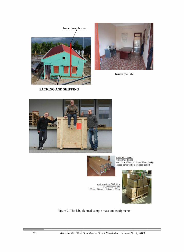
VI. CONSTRUCTION At present, NHMS is preparing for the lab, air-conditioner, electricity, internet and sample mast.
The instrument is packed and shipped to Viet Nam in 4 December 2013. According to the announcement of Swiss Embassy, the instrument expected to Viet Nam in 22 December 2013.Installation works scheduled for February 2014. The Viet Namese side will transport equipment to Pha Din and collaboration with Swiss specialist to install the equipment.
The Pha Din Global Atmospheric monitoring station will go into operation in March 2014.
20
PACKIN
Asia-P
NG AND SHI
Figure 2
Pacific GAW G
IPPING
2. The lab, pl
Greenhouse G
lanned samp
Gases Newslett
I
le mast and e
ter Volume N
Inside the lab
equipments
No. 4, 2013
b
Asia-Pacific GAW Greenhouse Gases Newsletter Volume No. 4, 2013 21
References
[1] The Project CATCOS (Capacity Building and Twinning for Climate Observing Systems). [2] Dr. Nicolas Bukowiecki, PSI and Dr. JörgKlausen,MeteoSwiss.First Viet Nam Visit of Swiss
CATCOS Delegation June 12-20, 2012. [3] Memorandum of Understanding (MOU) between Federal Office of Meteorology and Climatology
Meteoswiss and National Hydro-Meteorological Service of Viet Nam (NHMS) with reference to the project CATCOS signed in 27 May 2013.

22 Asia-Pacific GAW Greenhouse Gases Newsletter Volume No. 4, 2013
Preliminary Results of Greenhouse Gases Observed at Lulin Atmospheric Background Station (LABS), Taiwan
Chang-Feng Ou-Yang1,2, Neng-Huei Lin1, Jia-Lin Wang2, and Guey-Rong Sheu1
1. Department of Atmospheric Sciences, National Central University, Chungli-320, Taiwan
2. Department of Chemistry, National Central University,Chungli-320, Taiwan
Introduction
The island of Taiwan is situated in a unique position in East Asia in terms of observing pollution outflows from Southeast Asia and the Asian continent. Regional meteorological conditions are favorable for the transport of air pollutants, such as dusts, acidic pollutants, and biomass burning emissions, from upwind source regions to Taiwan [1], [2]. Thus, a high-elevation baseline station, Lulin Atmospheric Background Station (LABS), was established to measure baseline air pollutants and to study the atmospheric transport patterns. Official operation of LABS began on April 13, 2006, following the operating protocols of UN/WMO/GAW and US/NOAA/GMD sites. This station offers a great deal of opportunities to investigate the atmospheric chemistry of trace gases, aerosols, precipitation, mercury, and radiations, providing a distinctive contrast of atmospheric changes and impacts by a variety of air masses originated from relatively clean to emission source regions.
Site Description and Instrumentation
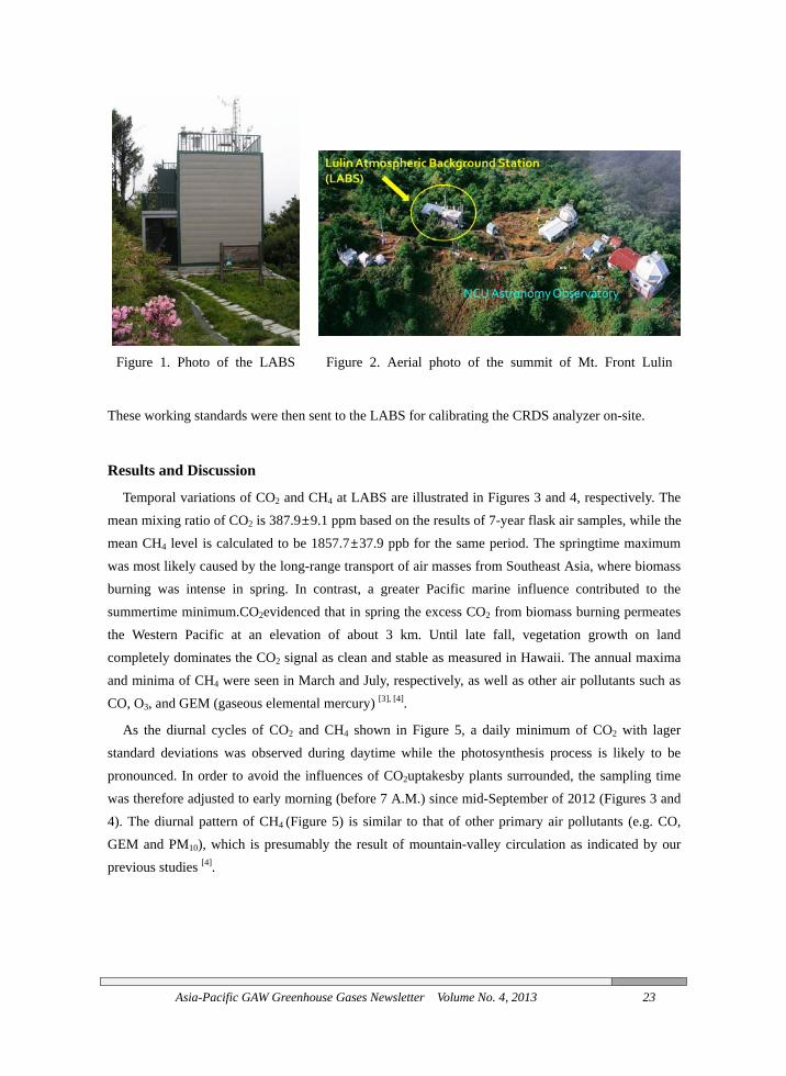
Lulin Atmospheric Background Station (23.47°N, 120.87°E; 2,862 m a.s.l.) is a two-story building (Figure 1) sitting on the summit of Mt. Front Lulin (Figure 2) in the Yu-Shan National Park in central Taiwan. The Lulin Astronomy Observatory is also located on the summit. There are no known point emission sources at the summit or in the surrounding area. The station is frequently within the free troposphere and is therefore an ideal site for making regional background air measurements. All of the instruments were placed on the second floor of the building, with the air intake line extruding to the roof and the inlet point approximately 10 m above ground. The instrument room is air-conditioned to keep constant air temperature around 25 ℃. More detailed descriptions of the LABS can be found in the literature [3].
Flask air sampling of GHGs were performed once a week by a NOAA/GMD’s PSU at LABS and Dongsha Island (20.70˚N, 116.73˚E; 8 m a.s.l.) since August 2006 and March 2010, respectively, measuring CO2, CH4, CO, N2O, SF6, H2, and isotopes (CO2
13C and CO218O). A cavity ring-down
spectroscopy (CRDS, Picarro G1301) analyzer continuously measures CO2 and CH4 at LABS since March 2011. Seven tertiary standard cylinders of CO2 (369.86 ppm, 391.99 ppm, 409.23 ppm, 516.30 ppm) and CH4 (1599.74 ppb, 1801.44 ppb, and 2024.64 ppb) purchased from NOAA/GMD were considered as our primary to verify the CO2 and CH4 mixing ratios in the working standards.
Asia-Pacific GAW Greenhouse Gases Newsletter Volume No. 4, 2013 23
Figure 1. Photo of the LABS Figure 2. Aerial photo of the summit of Mt. Front Lulin
These working standards were then sent to the LABS for calibrating the CRDS analyzer on-site.
Results and Discussion
Temporal variations of CO2 and CH4 at LABS are illustrated in Figures 3 and 4, respectively. The mean mixing ratio of CO2 is 387.9±9.1 ppm based on the results of 7-year flask air samples, while the mean CH4 level is calculated to be 1857.7±37.9 ppb for the same period. The springtime maximum was most likely caused by the long-range transport of air masses from Southeast Asia, where biomass burning was intense in spring. In contrast, a greater Pacific marine influence contributed to the summertime minimum.CO2evidenced that in spring the excess CO2 from biomass burning permeates the Western Pacific at an elevation of about 3 km. Until late fall, vegetation growth on land completely dominates the CO2 signal as clean and stable as measured in Hawaii. The annual maxima and minima of CH4 were seen in March and July, respectively, as well as other air pollutants such as CO, O3, and GEM (gaseous elemental mercury) [3], [4].
As the diurnal cycles of CO2 and CH4 shown in Figure 5, a daily minimum of CO2 with lager standard deviations was observed during daytime while the photosynthesis process is likely to be pronounced. In order to avoid the influences of CO2uptakesby plants surrounded, the sampling time was therefore adjusted to early morning (before 7 A.M.) since mid-September of 2012 (Figures 3 and 4). The diurnal pattern of CH4 (Figure 5) is similar to that of other primary air pollutants (e.g. CO, GEM and PM10), which is presumably the result of mountain-valley circulation as indicated by our previous studies [4].

24 Asia-Pacific GAW Greenhouse Gases Newsletter Volume No. 4, 2013
2006 2007 2008 2009 2010 2011 2012 2013 2014360
370
380
390
400
410
420
430
CO
2 (p
pm)
Time (UTC+8)
CRDS
Canister Canister_P
Figure 3. Time-series CO2 observed at LABS since August 2006. Open squares represent the preliminary results of NOAA/GMD flask air samples. Green lines represent the continuous CO2 data
measured by CRDS.
2006 2007 2008 2009 2010 2011 2012 2013 20141700
1750
1800
1850
1900
1950
2000
2050
2100
CH
4 (p
pb)
Time (UTC+8)
CRDS
Canister Canister_P
Figure 4. Time-series CH4 observed at LABS since August 2006. Open squares represent the
preliminary results of NOAA/GMD flask air samples. Brown lines represent the continuous CH4 data measure by CRDS.

Asia-Pacific GAW Greenhouse Gases Newsletter Volume No. 4, 2013 25
Hour
0 1 2 3 4 5 6 7 8 9 10 11 12 13 14 15 16 17 18 19 20 21 22 23
CO
2 (p
pm)
380
385
390
395
400
405
CH
4 (p
pb)
1800
1830
1860
1890
1920
1950CO2 CH4
Figure 5. Diurnal patterns of CO2 and CH4 observed at LABS, averaged from March 2011 to July 2013.
LABS provide comprehensive and informative results of GHG measurements at 3 km elevation in the Western Pacific, which is not only sufficiently representative of the hemispheric background levels, but also responsive to the regional large-scale burning activities in Southeast Asia.
References
[1] Lin NHet al.(1999). Evaluation of the characteristics of acid precipitation in Taipei, Taiwan using cluster analysis, Water Air and Soil Pollution, 113, 241-260.
[2] Wai KM et al. (2008). Rainwater chemistry at a high-altitude station, Mt. Lulin, Taiwan: comparison with a background station, Mt. Fuji, JGR-Atmospheres, 113(D6), doi:10.1029/2006JD008248.
[3] Sheu GR et al. (2009). Lulin Atmospheric Background Station: A New High-Elevation Baseline Station in Taiwan, EarozoruKenyu, 24(2), 84-89.
[4] Ou-Yang CF et al. (2012) Seasonal and diurnal variations of ozone at a high-altitude mountain baseline station in East Asia, Atmospheric Environment, 46, 279-288.

26 Asia-Pacific GAW Greenhouse Gases Newsletter Volume No. 4, 2013
Development of Southeast Asia-Australian Atmospheric Observation Capability
M. V. van der Schoot, B. Atkinson, P.J. Fraser, J. Ward, M. Keywood, P. B. Krummel Centre for Australian Weather and Climate Research, CSIRO Marine and Atmospheric Research
In collaboration with a range of partners, Australia’s Centre for Australian Weather and Climate
Research (CAWCR) at CSIRO Marine and Atmospheric Research, is developing an integrated atmospheric observation network for greenhouse gases (GHG) and other climatically-active atmospheric species in the Southeast Asia-Australian region. This network is an extension of the Australian Greenhouse Gas Observation Network (AGGON) which has the Cape Grim Baseline Air Pollution Station (CGBAPS) as the central reference site. CGBAPS is a Global Atmospheric Watch (GAW) global station and one of only three designated “comparison” sites for GHG in the network.
The objectives of the expansion of the AGGON network are to:
1. Establish a continental Australian network to develop “top-down” emission verification tools (e.g. Australian coal seam gas fugitive emissions applications);
2. Understand key atmospheric processes in the Australian-Southeast Asian tropical region; 3. Quantify the changing Southern Ocean CO2 sink, and 4. Exploit new research platforms – Australian blue water research vessel RV Investigator
(expected to be operational early 2014)
Understanding the globally significant tropical atmospheric processes is a key focus of this research activity and therefore the expansion of the research capability in this region is an important step.
Currently the Southeast Asia-Australian tropical regional network includes two GAW global stations (Bukit Kota Tabang, Indonesia and Danum Valley, Malaysia) as well as more than ten other air sampling sites for GHG (Figure 1).
The main Australian contribution to this network is the development of the Australian Tropical Atmospheric Research Station (ATARS) at Gunn Point in Australia’s Northern Territory – a GAW regional station in the Australian tropical savannah region (Figure 2). In the dry season (Austral winter) the prevailing synoptic easterly winds expose this site to the significant biomass burning events that regularly occur in the large expanse of the Australian tropical savannah. In the monsoon season (Austral summer) the Gunn Point site is exposed to air masses originating from the Southeast Asian region.

Asia-Pacific GAW Greenhouse Gases Newsletter Volume No. 4, 2013 27
Figure 1. Southeast Asia-Australian tropical regional GHG observation network
Figure 2. Gunn Pt site with new 2nd container laboratory
The research program at Gunn Pt ATARS has developed significantly over the last year (Table 1) with significant expansion of the available laboratory space with a new 2nd container laboratory, and the installation of new equipment. This includes the installation of: a GC-ECD system to study short-lived halocarbons from marine biogenic sources (University of Cambridge, UK); an automatic weather station (AWS), and an Aerosol Diffusion Dryer (ARADD) system including ambient MET sensors on tower and an ultra-Dry 10Bar compressed air system.
An example of the data collected so far from the Gunn Pt site is shown in Figure 3 showing the time series of a range of greenhouse and related traces gases and isotopes from the flask air sample collection program. These results can be compared with the time series that have been collected at Cape Ferguson (East coast of Australia) (Figure 3).

28 Asia-Pacific GAW Greenhouse Gases Newsletter Volume No. 4, 2013
Table 1. Gunn Point ATARS atmospheric measurement program
Atmospheric species / technique Research Group Period of Operation
In-situ CO2 & CH4 (CRDS) CAWCR/CMAR (2011 - present)
In-situ 13CO2/12CO2 (CRDS) CAWCR/CMAR (2011-2012)
Flask CO2, CH4,13CO2/12CO2, N2O, CO, H2 CAWCR/CMAR (2011 – present)
Radon-222 ANSTO (2011 – present)
Short-lived halocarbons (CHBr3/CH2Br2/CHCl3/C2Cl4/CH2CCl3/CCl4..) GC-ECD
University of Cambridge (UK)
(Jul 2013 – present)
Automatic Weather Station
(with 2nd anemometer on tower since 2011)
CAWCR/CMAR (Jul 2013 - present)
O3 (UV spectrometry) CAWCR/CMAR (2011 – present)
CO (NDIR) /NO/NOX (chemiluminescence) CAWCR/CMAR (2011-2012)
Aerosols (nephelometer) CAWCR/CMAR (2011 – 2013)
Aerosols (absorption photometer) CAWCR/CMAR (2011 – 2012)
Proposed measurement program (NEW container lab)
In-situ CO/N2O (Off-axis ICOS) CAWCR/CMAR (May/June 2014)
CO/NO/NOX CAWCR/CMAR (May/June 2014)
PM2.5/PM10 CAWCR/CMAR (May/June 2014)
Aerosols & VOCs CAWCR/CMAR (May/June 2014)
Asia-Pacific GAW Greenhouse Gases Newsletter Volume No. 4, 2013 29
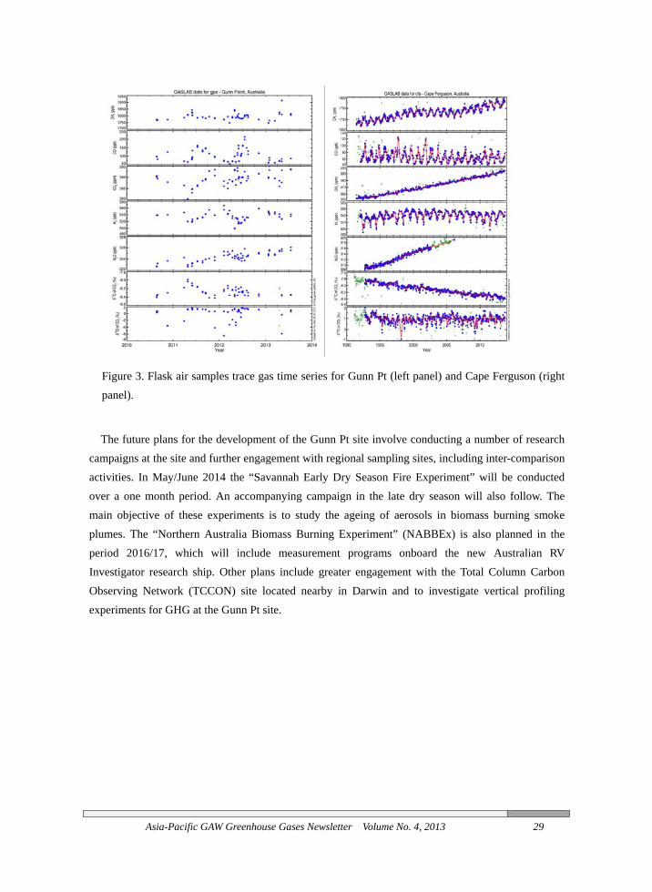
Figure 3. Flask air samples trace gas time series for Gunn Pt (left panel) and Cape Ferguson (right panel).
The future plans for the development of the Gunn Pt site involve conducting a number of research campaigns at the site and further engagement with regional sampling sites, including inter-comparison activities. In May/June 2014 the “Savannah Early Dry Season Fire Experiment” will be conducted over a one month period. An accompanying campaign in the late dry season will also follow. The main objective of these experiments is to study the ageing of aerosols in biomass burning smoke plumes. The “Northern Australia Biomass Burning Experiment” (NABBEx) is also planned in the period 2016/17, which will include measurement programs onboard the new Australian RV Investigator research ship. Other plans include greater engagement with the Total Column Carbon Observing Network (TCCON) site located nearby in Darwin and to investigate vertical profiling experiments for GHG at the Gunn Pt site.

30
Gor
Backgr
The ssouthernHowevethe specdominatland useOcean punresolvSouthernof Wateregion tundersta
Figur
For
rdon Brailsfo
1. Nation2.
round
sources of can hemisphereer the trends cies is long ted by oceane change andplaying an eved for the cn Ocean carb
er and Atmothat provide anding carbo
re 1. Baring
Asia-P
rty YearB
ord1, Britton
nal Institute oNational Ce
arbon dioxide, resulting iin the atmoslived and trs. Nearly a qd other humaespecially c
carbon cyclesbon sink, andospheric Res
trace-gas obn cycle proc
Head stationand is fre
Pacific GAW G
s of Basearing HStephens2, S
John McG
of Water andenter for Atm
Gordon.B
e (CO2) emiin inter-hemspheric CO2
ransported toquarter of thean activities
critical role s that are lind uptake by earch (NIWAbservations, esses.
n is located oquently expo
Greenhouse G
eline COead, New
Sara Mikaloff
regor1, Kay
d Atmospherimospheric Res
Brailsford@n
issions are grmispheric diff
are comparao the south. e CO2 emittehas been abin the carbo
nked to southsouthern hem
WA) maintaincompatible
on the southeosed to basel
Gases Newslett
O2 Measuw Zealanff Fletcher1, S
Steinkamp1
ic Research, search, Boul
niwa.co.nz
reater in theferences of aable between
The southeed to the atmbsorbed by eon cycle. Shern hemisphmisphere lann a network
with other G
ern tip of the line air from
ter Volume N
urementnd
Sylvia Nicho
Wellington, lder Colorad
northern heatmospheric n hemisphereern hemisphe
mosphere fromearth’s oceaneveral critichere process
nd masses). Tof stations
GAW station
North Islandthe south.
No. 4, 2013
ts at
ol1, Katja Rie
New Zealando, USA
emisphere thCO2 mole f
es due to the ere geographm fossil fuel ns, with the cal questionsses (e.g. trenThe Nationalin the New
ns, that cont
d (Te Ika-a-M
edel1,
d.
an in the fractions. fact that
hically is burning, Southern
s remain nds in the l Institute
Zealand tribute to
Maui),
Asia-Pacific GAW Greenhouse Gases Newsletter Volume No. 4, 2013 31
Baring Head observations
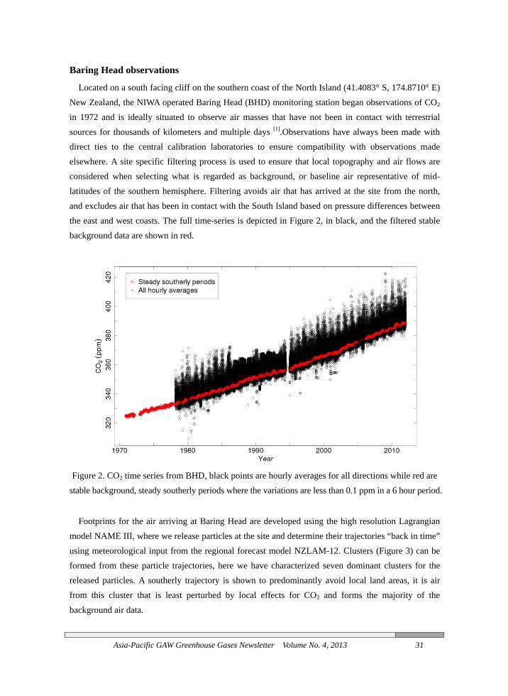
Located on a south facing cliff on the southern coast of the North Island (41.4083° S, 174.8710° E) New Zealand, the NIWA operated Baring Head (BHD) monitoring station began observations of CO2 in 1972 and is ideally situated to observe air masses that have not been in contact with terrestrial sources for thousands of kilometers and multiple days [1].Observations have always been made with direct ties to the central calibration laboratories to ensure compatibility with observations made elsewhere. A site specific filtering process is used to ensure that local topography and air flows are considered when selecting what is regarded as background, or baseline air representative of mid-latitudes of the southern hemisphere. Filtering avoids air that has arrived at the site from the north, and excludes air that has been in contact with the South Island based on pressure differences between the east and west coasts. The full time-series is depicted in Figure 2, in black, and the filtered stable background data are shown in red.
Figure 2. CO2 time series from BHD, black points are hourly averages for all directions while red are stable background, steady southerly periods where the variations are less than 0.1 ppm in a 6 hour period.
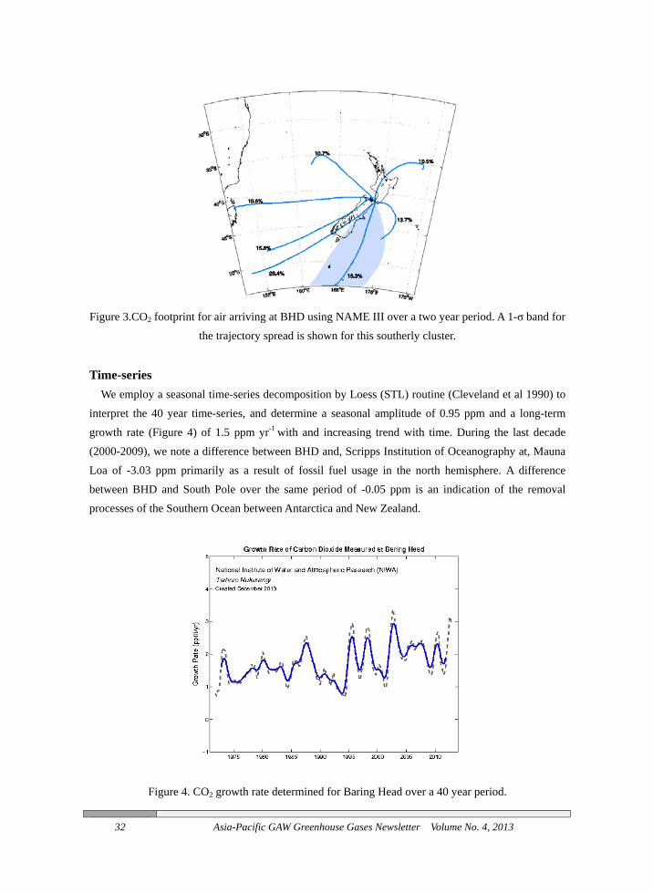
Footprints for the air arriving at Baring Head are developed using the high resolution Lagrangian model NAME III, where we release particles at the site and determine their trajectories “back in time” using meteorological input from the regional forecast model NZLAM-12. Clusters (Figure 3) can be formed from these particle trajectories, here we have characterized seven dominant clusters for the released particles. A southerly trajectory is shown to predominantly avoid local land areas, it is air from this cluster that is least perturbed by local effects for CO2 and forms the majority of the background air data.
32 Asia-Pacific GAW Greenhouse Gases Newsletter Volume No. 4, 2013
Figure 3.CO2 footprint for air arriving at BHD using NAME III over a two year period. A 1-σ band for
the trajectory spread is shown for this southerly cluster.
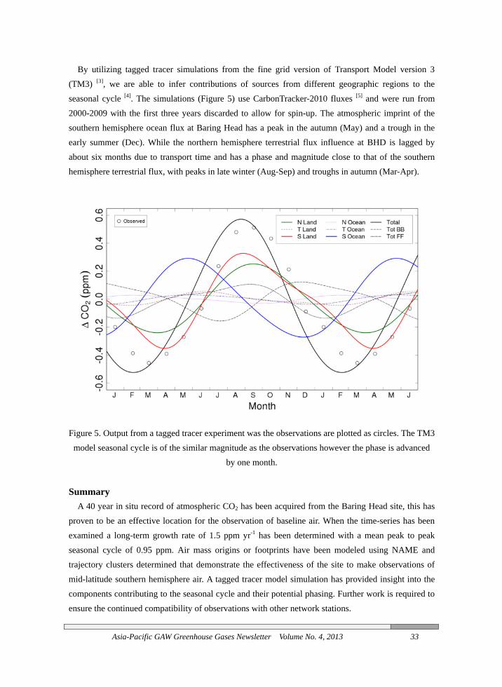
Time-series We employ a seasonal time-series decomposition by Loess (STL) routine (Cleveland et al 1990) to
interpret the 40 year time-series, and determine a seasonal amplitude of 0.95 ppm and a long-term growth rate (Figure 4) of 1.5 ppm yr-1 with and increasing trend with time. During the last decade (2000-2009), we note a difference between BHD and, Scripps Institution of Oceanography at, Mauna Loa of -3.03 ppm primarily as a result of fossil fuel usage in the north hemisphere. A difference between BHD and South Pole over the same period of -0.05 ppm is an indication of the removal processes of the Southern Ocean between Antarctica and New Zealand.
Figure 4. CO2 growth rate determined for Baring Head over a 40 year period.
Asia-Pacific GAW Greenhouse Gases Newsletter Volume No. 4, 2013 33
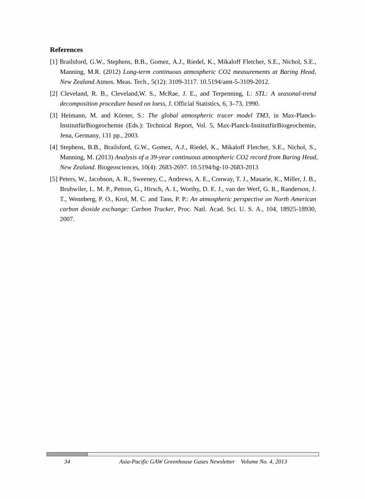
By utilizing tagged tracer simulations from the fine grid version of Transport Model version 3 (TM3) [3], we are able to infer contributions of sources from different geographic regions to the seasonal cycle [4]. The simulations (Figure 5) use CarbonTracker-2010 fluxes [5] and were run from 2000-2009 with the first three years discarded to allow for spin-up. The atmospheric imprint of the southern hemisphere ocean flux at Baring Head has a peak in the autumn (May) and a trough in the early summer (Dec). While the northern hemisphere terrestrial flux influence at BHD is lagged by about six months due to transport time and has a phase and magnitude close to that of the southern hemisphere terrestrial flux, with peaks in late winter (Aug-Sep) and troughs in autumn (Mar-Apr).
Figure 5. Output from a tagged tracer experiment was the observations are plotted as circles. The TM3 model seasonal cycle is of the similar magnitude as the observations however the phase is advanced
by one month.
Summary A 40 year in situ record of atmospheric CO2 has been acquired from the Baring Head site, this has
proven to be an effective location for the observation of baseline air. When the time-series has been examined a long-term growth rate of 1.5 ppm yr-1 has been determined with a mean peak to peak seasonal cycle of 0.95 ppm. Air mass origins or footprints have been modeled using NAME and trajectory clusters determined that demonstrate the effectiveness of the site to make observations of mid-latitude southern hemisphere air. A tagged tracer model simulation has provided insight into the components contributing to the seasonal cycle and their potential phasing. Further work is required to ensure the continued compatibility of observations with other network stations.
34 Asia-Pacific GAW Greenhouse Gases Newsletter Volume No. 4, 2013
References
[1] Brailsford, G.W., Stephens, B.B., Gomez, A.J., Riedel, K., Mikaloff Fletcher, S.E., Nichol, S.E., Manning, M.R. (2012) Long-term continuous atmospheric CO2 measurements at Baring Head, New Zealand.Atmos. Meas. Tech., 5(12): 3109-3117. 10.5194/amt-5-3109-2012.
[2] Cleveland, R. B., Cleveland,W. S., McRae, J. E., and Terpenning, I.: STL: A seasonal-trend decomposition procedure based on loess, J. Official Statistics, 6, 3–73, 1990.
[3] Heimann, M. and Körner, S.: The global atmospheric tracer model TM3, in Max-Planck-InstitutfürBiogeochemie (Eds.): Technical Report, Vol. 5, Max-Planck-InstitutfürBiogeochemie, Jena, Germany, 131 pp., 2003.
[4] Stephens, B.B., Brailsford, G.W., Gomez, A.J., Riedel, K., Mikaloff Fletcher, S.E., Nichol, S., Manning, M. (2013) Analysis of a 39-year continuous atmospheric CO2 record from Baring Head, New Zealand. Biogeosciences, 10(4): 2683-2697. 10.5194/bg-10-2683-2013
[5] Peters, W., Jacobson, A. R., Sweeney, C., Andrews, A. E., Conway, T. J., Masarie, K., Miller, J. B., Bruhwiler, L. M. P., Petron, G., Hirsch, A. I., Worthy, D. E. J., van der Werf, G. R., Randerson, J. T., Wennberg, P. O., Krol, M. C. and Tans, P. P.: An atmospheric perspective on North American carbon dioxide exchange: Carbon Tracker, Proc. Natl. Acad. Sci. U. S. A., 104, 18925-18930, 2007.
The G
M
Monito
The Gsuch as monitori
This related tresearchthrough focus top
Greenh
SinceOrganisaconcentrcomprisreferencdried usminute b
Asia-Pac
Greenho
MMalaysian Me
oring Activi
GAW monitoaerosol, greeing activities
paper will oto greenhou
h findings baMet Malayspic will be fu
ouse Gases
e 2004, Met Mation (CSIRration contines 10 minute
ce cells of thsing the Nafiblocks are u
cific GAW Gre
ouse Gas
Mohd Firdauseteorological
ities
oring activitenhouse gass at GAW sta
Table 1. The
only focus ouse gases moased on the dsia’s collaborurther discus
Malaysia hasRO), Australnuously at Des measuremhe LI-COR),ion dryer (ba
used to provi
eenhouse Gase
es Obser
ins Jahaya, MazDepartment, J
ies at GAW es, reactive
ations in Mal
e monitoring
on the on-goonitoring pr
data analysis ration with ossed as follow
s collaboratelia in instalDanum Vall
ment on the R followed byacked up by ide ample op
es Newsletter
rvation a
n Malaysznorizan MoJalan Sultan,
stations in gases, O3, Ulaysia are as
g activities at
oing greenhrogrammes aare discusse
other researcws:
ed with Commlling a LoFley GAW SREF cylindey 50 minutethe mop-up
pportunity fo
Volume No.
and Ana
sia ohamad, and 46667 Petalin
Malaysia foUV radiation
listed in Tab
t GAW statio
house gases at GAW stated in this papch agencies.
monwealth SFlo Mark II tation. In thr (REF cylin
es measuremdryer). The
or flow and p
. 4, 2013
alysis at G
Toh Ying Ying Jaya, Selan
cuses on sixand precipit
ble 1.
ons in Malays
and selectedtions in Maper, includingSeveral para
Scientific andCO2Analyz
he monitorinnder air throu
ment of ambifirst 6 minu
pressure stab
GAW sta
ing ngor, Malaysia
x classes of vtation chemi
sia.
d reactive gaalaysia. Somg research coameters relat
d Industrial Rzer to moning mode, eaugh both sament air that utes of the 1bilisation; th
35
ations
a
variables stry. The
ases that me of the
onducted ted to the
Research itor CO2 ach hour mple and has been 0 and 50
hus ‘valid
36
data’ comobtainedand dataweeks, w
On thStudies, method (every Sto NIESNIES.
Reactiv
Surfausing Thozone (O3Analygases su
Result Carbon
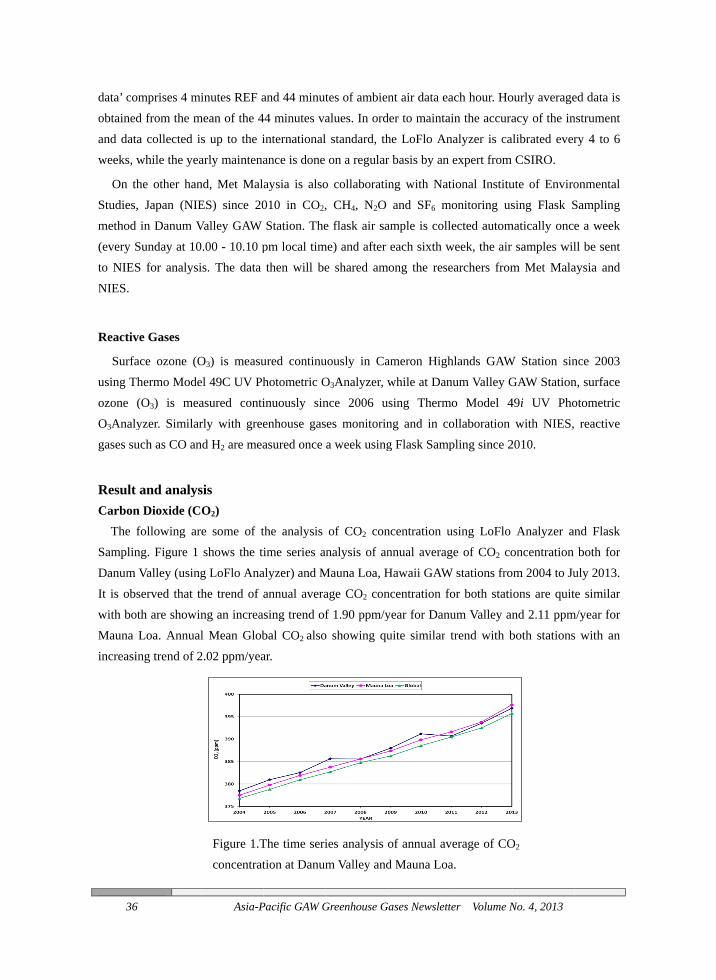
The fSamplinDanum VIt is obswith botMauna Lincreasin
mprises 4 mid from the ma collected iswhile the yea
he other hanJapan (NIE
in Danum VSunday at 10S for analysi
e Gases
ace ozone (Ohermo Mode(O3) is meayzer. Similaruch as CO an
and analysn Dioxide (Cfollowing arng. Figure 1 Valley (usingserved that thth are showinLoa. Annualng trend of 2
Asia-P
inutes REF amean of the 4
s up to the iarly maintena
nd, Met MalES) since 20Valley GAW 0.00 - 10.10 pis. The data
O3) is measuel 49C UV Phasured contirly with gree
nd H2 are mea
sis O2) e some of tshows the ti
g LoFlo Anahe trend of ang an increal Mean Glob
2.02 ppm/yea
Figure 1.Tconcentrat
Pacific GAW G
and 44 minut44 minutes vainternationalance is done
aysia is also010 in CO2,Station. The
pm local timthen will be
ured continuhotometric Oinuously sinenhouse gasasured once
the analysis ime series a
alyzer) and Mannual averasing trend ofbal CO2 alsoar.
The time serition at Danum
Greenhouse G
tes of ambienalues. In ordl standard, thon a regular
o collaborati, CH4, N2O e flask air sa
me) and after e shared am
uously in CaO3Analyzer, wnce 2006 uses monitorina week using
of CO2 connalysis of an
Mauna Loa, Hage CO2 conf 1.90 ppm/y
o showing qu
ies analysis m Valley and
Gases Newslett
nt air data eader to maintahe LoFlo Anr basis by an
ng with Natand SF6 m
ample is colleach sixth w
mong the rese
ameron Highwhile at Dan
using Thermng and in cog Flask Samp
ncentration unnual averagHawaii GAWncentration foyear for Danuuite similar
of annual avd Mauna Loa
ter Volume N
ach hour. Hoain the accuranalyzer is caexpert from
tional Institumonitoring uslected automweek, the air earchers from
hlands GAWnum Valley G
mo Model 4ollaboration pling since 2
using LoFlo ge of CO2 co
W stations frofor both statium Valley antrend with b
verage of COa.
No. 4, 2013
ourly averageacy of the in
alibrated everCSIRO.
ute of Envirosing Flask S
matically oncesamples wil
m Met Mala
W Station sinGAW Station49i UV Pho
with NIES,2010.
Analyzer anoncentration
om 2004 to Juions are quitnd 2.11 ppmboth stations
O2
ed data is nstrument ry 4 to 6
onmental Sampling e a week ll be sent aysia and
nce 2003 n, surface otometric reactive
nd Flask both for
uly 2013. te similar
m/year for s with an

FigureSamplinconcentrFrom thonly less
Other GThe fo
N2O & GAW St5, 6 andSamplinflask air4 days. Iquite simthroughobefore Nhigh befbecome concentrN2O (32average Danum between
Asia-Pac
e 2 shows thng from Junration by Lo
he comparisos than 5% pe
FigureLoFlo
Greenhouse following anaSF6) and reatation) and cd 7 shows thng at Danumr sample is coIt is observedmilar with Nout the perioNovember 20fore Novemb
more comprations of the22.5 - 327.0
values as iValley range
n 536.04 - 1,1
cific GAW Gre
he comparisne 2011 to JoFlo Analyzeon, the valueercentage diffference.
e 2. The oAnalyzer an
Gases (CH4
alysis will tryactive gases coastal area ihe time serie
m Valley and ollected autod that the tre
N2O and SF6
od from Janu012 for Danuber 2012 becparable to tese three gre
04 ppb) and issued by thed between 127.25 ppb.
eenhouse Gase
on of CO2 cJune 2013 aer is chosen es from the b
comparisonnd Flask Sam
, N2O & SF6
y to explain (CO & H2) cin temperate es analysis oHateruma (a
omatically onends of CH4,
6 are showinuary 2010 toum Valley. Tause of contthe Haterumenhouse gasSF6 (6.99 -
he 2012WM73.5 - 249.7
es Newsletter
concentrationat Danum Vfrom the samboth method
n of CO2
mpling.
6) and Reactthe trend andconcentratiozone (Haterf CH4, N2O,as a referencnce a week aN2O, SF6, C
ng slight inco June 2013. The value fotamination fr
ma after newes at Danum8.25 ppt) a
MO Greenhou72 ppb, whil
Volume No.
n measured uValley GAW me hour of ss are showin
concentratio
tive Gases (Cd time seriesns at rainfor
ruma, Japan c, SF6, CO ance site) from t Danum Val
CO and H2 coreasing trenH2 is showi
or H2 concenrom Flask Saw pump is
m Valley, namare comparabuse Gas Bule H2 concen
. 4, 2013
using LoFloStation. Th
ampling timng quite a co
on measure
CO & H2) s of some grerest in the trocontributing nd H2 concenJanuary 201
lley, while atoncentrationsd, while CHing stable trentration at Dampling’s oldchanged in
mely CH4 (1,7ble with thelletin. The Cntration at D
o Analyzer ahe hourly m
me of Flask Somparable tr
ed using
eenhouse gasopics (Danumstation). Fig
ntrations usi10 to June 2t Hateruma is for both sta
H4 and CO fend except foanum Valleyd pump and t
October 20792.35 - 1,94e range of thCO concent
Danum Valle
37
and Flask mean CO2 Sampling. rend with
ses (CH4, m Valley gure 3, 4, ing Flask 013. The s once in
ations are fluctuates or period y is quite the value 012. The 42.5 ppb), he global tration at y ranged

38
Figure concentr
Figure concentr
3.The timeration at Dan
5.The timeration at Dan
Asia-P
e series annum Valley a
e series annum Valley a
Figureconcen
Pacific GAW G
nalysis of Cand Hateruma
nalysis of and Hateruma
e 7.The tintration at D
Greenhouse G
CH4 a.
Figcon
SF6
a.
Figcon
ime series Danum Valley
Gases Newslett
gure 4.The ncentration at
gure 6.The ncentration at
analysis oy and Hateru
ter Volume N
time seriest Danum Val
time seriet Danum Val
of H2 uma.
No. 4, 2013
s analysis lley and Hate
es analysis lley and Hate
of N2O eruma.
of CO
eruma.
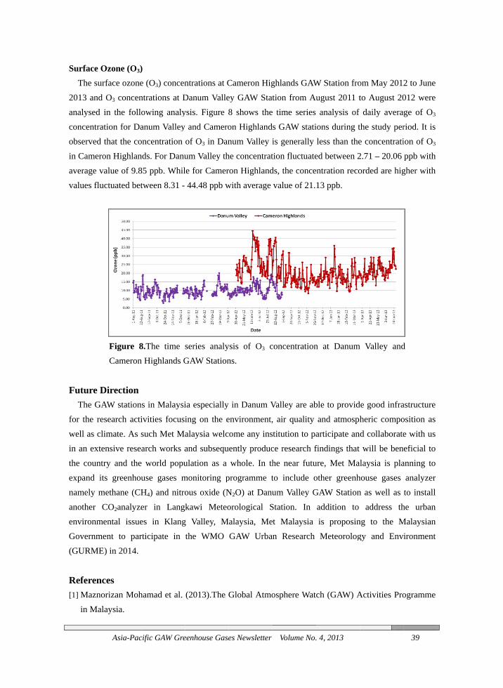
SurfaceThe su
2013 ananalysedconcentrobservedin Cameaverage values fl
Future The G
for the rwell as cin an exthe counexpand namely another environmGovernm(GURM
Referen[1] Mazn
in M
Asia-Pac
e Ozone (O3)urface ozone
nd O3 concend in the folloration for Dad that the coeron Highlanvalue of 9.8
fluctuated bet
Figure 8Cameron
Direction GAW stationresearch acticlimate. As s
xtensive resentry and theits greenhoumethane (CHCO2analyze
mental issuement to par
ME) in 2014.
nces norizan Mohalaysia.
cific GAW Gre
) e (O3) concenntrations at Dowing analyanum Valleyoncentration nds. For Danu85 ppb. Whiltween 8.31 -
8.The time n Highlands G
ns in Malaysiivities focusisuch Met Maarch works a
e world popuuse gases mH4) and nitroer in Langes in Klangrticipate in
hamad et al.
eenhouse Gase
ntrations at CDanum Valleysis. Figure 8y and Cameroof O3 in Danum Valley thle for Camer44.48 ppb w
series analyGAW Station
ia especially ing on the ealaysia welcand subsequulation as a monitoring pous oxide (Nkawi Meteo
g Valley, Mthe WMO
(2013).The G
es Newsletter
Cameron Higey GAW Stat8 shows theon Highlandnum Valley i
he concentratron Highlandwith average
ysis of O3 cns.
in Danum Venvironment,ome any ins
uently producwhole. In th
programme tN2O) at Danuorological Salaysia, MeGAW Urba
Global Atmo
Volume No.
ghlands GAWtion from Au
e time series s GAW statiis generally tion fluctuateds, the concevalue of 21.
concentration
Valley are ab, air quality stitution to pace research fhe near fututo include oum Valley G
Station. In et Malaysia n Research
osphere Wat
. 4, 2013
W Station frougust 2011 tanalysis of
ions during tless than the
ed between 2entration reco13 ppb.
n at Danum
ble to providand atmospharticipate anfindings that ure, Met Maother greenhGAW Stationaddition to is proposinMeteorolog
ch (GAW) A
om May 2012to August 20
f daily averathe study pere concentrati2.71 – 20.06 orded are hig
m Valley and
de good infraheric compod collaboratewill be ben
laysia is plahouse gases n as well as
address thng to the Mgy and Env
Activities Pro
39
2 to June 012 were ge of O3 riod. It is ion of O3 ppb with
gher with
d
astructure osition as e with us eficial to
anning to analyzer to install
he urban Malaysian
ironment
ogramme
40 Asia-Pacific GAW Greenhouse Gases Newsletter Volume No. 4, 2013
[2] Maznorizan Mohamad et al. (2012).The Measurement and Analysis of Greenhouse Gases at GAW Station in Danum Valley, Malaysia, Asian GAW Greenhouse Gases Newsletter, Volume No. 3: 22-30.
[3] Maznorizan Mohamad et al. (2011).The Global Atmosphere Watch (GAW) Activities in Malaysia, Asian GAW Greenhouse Gases Newsletter, Volume No. 2: 21-26.
[4] WMO WDCGG Data Summary, WDCGG No. 37, GAW Data, Volume IV-Greenhouse Gases and Other Atmospheric Gases (2013).
[5] WMO Greenhouse Gas Bulletin (2012). [6] Earth System Research Laboratory (NOAA) Global Monitoring Division.
http://www.esrl.noaa.gov/gmd/ccgg/trends
Asia-Pacific GAW Greenhouse Gases Newsletter Volume No. 4, 2013 41
Gravimetric standards of Greenhouse gases at ambient levels
JeongSik Lim1, Jin Bok Lee1, Haeyoung Lee2,Dong Min Moon1,Miyeon Park1, A-rang Lim1, Jeong Soon Lee1,*
1. Center for gas analysis, Korea Research Institute of Standards and Science
2. Korea Meteorology Administration
1. Introduction
The Global Atmosphere Watch (GAW) Programme of the World Meteorological Organization (WMO) serves as an international framework aimed at maintaining the traceability chain for Greenhouse Gases observation passing through the Central Calibration Centre (CCL) and World Calibration Centre (WCC). The Korea Research Institute of Standards and Science (KRISS) and the Korea Meteorology Administration (KMA) agreed to host WCC-SF6(World Calibration Center for SF6) and started to improve the analytical capability of SF6.[1]
In this newsletter, we present new gravimetric standard scales of SF6 for supporting WCC task. Furthermore, N2O scale will be introduced. Each standard was developed according to the ISO 6142. [2] And the uncertainties of prepared cylinders are individually evaluated to meet virtually no errors on the regression of the sets of standards covering ambient levels. We hope this primary scale will contribute to strengthen the WMO traceability chain. Therefore, the comparison of KRISS and NOAA scale is planned in order to ensure the equivalence between them. Before leaving this letter, the comparison of CO2, CH4 standard will be also introduced to report the deviation between KRISS and NOAA standards.
2. Primary standards developments 2.1 Overview
In this letter, we will present our recent achievements on new standards of N2O in air and SF6in air. Impurity analysis of pure gases of SF6, N2O, N2, O2 and Ar were performed and every dilution steps are gravimetrically controlled according to ISO 6142. Particularly, SF6 of which mixing ratio at atmospheric is pmol/mol, careful investigation on SF6 impurity in air matrix was rigorously carried out to pick out sub-ppt level of SF6, which provides slightly positive bias on the certified mixing ratio. For this purpose, the pre-concentrator-GC-ECD was brought to ensure the SF6 trace in matrix. To verify dilution steps, analyses were performed using KRISS-calibrated gas chromatograph with thermal conductivity detector or electron capture detector (GC-TCD and ECD, respectively) according to ISO 6143.[3] For SF6/air scale, 5 cylinders were gravimetrically prepared as a function of mixing ratio in the range of ambient levels (5~15 pmol/mol). In case of N2O scale covering ambient
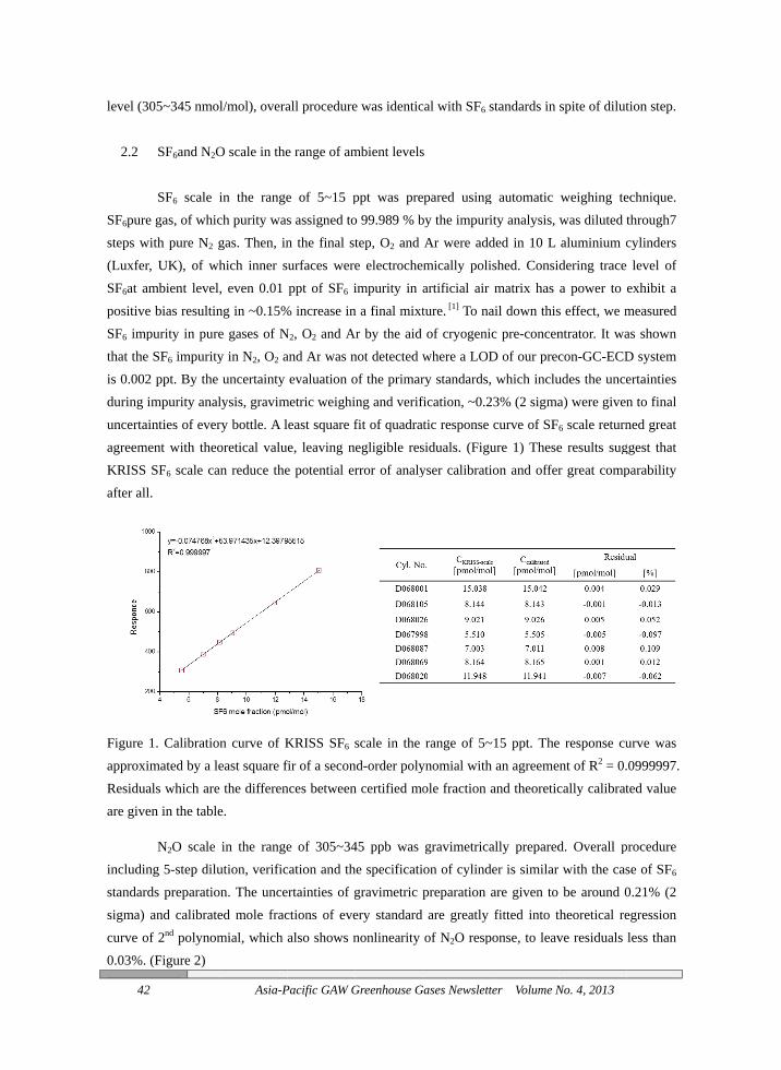
42
level (30 2.2
SF6pure steps wi(Luxfer,SF6at ampositive SF6 impthat the is 0.002 during imuncertaiagreemeKRISS after all.
Figure 1approximResiduaare given
includinstandardsigma) acurve of0.03%. (
05~345 nmo
SF6and N2O
SF6 scale igas, of whic
ith pure N2 g UK), of wh
mbient levelbias resultin
purity in pureSF6 impurityppt. By the
mpurity analnties of ever
ent with theoSF6 scale ca.
1. Calibratiomated by a lels which aren in the table
N2O scale ng 5-step diluds preparatioand calibratef 2nd polynom(Figure 2)
Asia-P
l/mol), overa
O scale in the
in the rangech purity wasgas. Then, inhich inner s, even 0.01 ng in ~0.15%e gases of Ny in N2, O2 auncertainty
lysis, gravimry bottle. A loretical valuan reduce the
n curve of Keast square f
e the differene.
in the rangeution, verificon. The unceed mole fracmial, which
Pacific GAW G
all procedure
e range of am
e of 5~15 ps assigned ton the final sturfaces wereppt of SF6 i
% increase inN2, O2 and Aand Ar was nevaluation o
metric weighileast square fe, leaving ne potential er
KRISS SF6 sfir of a seconnces between
e of 305~34cation and thertainties of gctions of evealso shows n
Greenhouse G
e was identic
mbient levels
ppt was preo 99.989 % btep, O2 and e electrocheimpurity in a
n a final mixtAr by the aid not detected wof the primaring and veriffit of quadrategligible resrror of analy
scale in the nd-order polyn certified mo
45 ppb was he specificatigravimetric pery standard nonlinearity
Gases Newslett
cal with SF6 s
s
epared usingby the impuriAr were addmically poliartificial air ture. [1] To naof cryogeni
where a LODry standards,fication, ~0.2tic response
siduals. (Figuyser calibrati
range of 5~ynomial withole fraction a
gravimetricaon of cylindpreparation aare greatly
of N2O resp
ter Volume N
standards in
g automatic ity analysis, ded in 10 L ished. Consimatrix has
ail down thisc pre-concenD of our prec, which inclu23% (2 sigma
curve of SFure 1) Theseion and offer
~15 ppt. Theh an agreemeand theoretic
ally preparedder is similar are given to fitted into t
ponse, to leav
No. 4, 2013
spite of dilut
weighing tewas diluted taluminium cdering tracea power to
s effect, we mntrator. It wacon-GC-ECDudes the uncea) were given
6 scale returne results sugr great comp
e response cuent of R2 = 0.cally calibrat
d. Overall pwith the casbe around 0
theoretical reve residuals
tion step.
echnique. through7 cylinders level of exhibit a
measured as shown D system ertainties n to final ned great
ggest that parability
urve was .0999997. ted value
procedure se of SF6 0.21% (2 egression less than
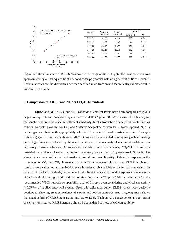
Figure 2approximResiduaare given
3. Com
degree omethanafollows.carrier g(referencparts of laboratoprovidedstandardsubstancstandardcase of KNOAA srecomm(<0.05 %overlappthat negof conve
Asia-Pac
2. Calibrationmated by a lels which aren in the table
mparison of
KRISS andof equivalenator was coup Porapak-Q gas was feece) gas mixtgas lines ar
ory pressure d by NOAAds are very wces of CO2 d were calibrKRISS CO2 standard is s
mended WMO%) of applieped, showingative bias ofersion factor
cific GAW Gre
n curve of KReast square f
e the differene.
f KRISS an
d NOAA COnce. Analyticpled to securcolumn for
ed with apprture, well cale protected btolerance. A
A as Central well scaled and CH4, itrated againststandards, p
straight and O network coed analyticalg great equivf KRISS stan
to KRISS st
eenhouse Gase
RISS N2O scfir of a seconnces between
d NOAA C
O2 and CH4 scal system wre sufficient CO2 and Moropriately adlibrated MFCby the restricAs referenceCalibration
and used ant seemed to t NOAA scaperfect matchresiduals areomparabilityl system. Upvalence of Kndard as muctandard shou
es Newsletter
cale in the rand-order polyn certified mo
CO2/CH4sta
tandards at awas GC-FIDsensitivity. Bolsieve 5A pdjusted flowC (Bronkhorsctor in case es for this cLaboratory
nalyzer showbe sufficien
ale in order th with NOAe given less y goal of 0.1 pon this cali
KRISS and Nch as ~0.13 %uld be consid
Volume No.
ange of 305~ynomial withole fraction a
andards
ambient leveD (Agilent 68Brief introdupacked columw rate. To lost) was coupof the necescomparison for CO2 an
ws great linently reasonabto give reliab
AA scale was than 0.07 ppppm even c
ibration curvNOAA standa%. (Table 2) ered to meet
. 4, 2013
345 ppb. Thh an agreemeand theoretic
els have been890A). In ca
uction of analmn for CH4woad constan
pled to samplssity of instru
analysis, Cd CH4 werearity of deteble that oneble result forfound. Resp
pm (Table 1considering ave, KRISS vards. But, CHAs a consequt WMO comp
e response cuent of R2 = 0cally calibrat
n compared ase of CO2 lytical condiwere appliednt amount ofling gas lineument isolatO2/CH4 gas
e used. Sinceector respone KRISS grar full compaponse curve ), which satianalytical unvalues were H4comparisouence, an appatibility.
43
urve was 0.099997. ted value
to give a analysis, tion is as
d. N2 as a f sample . Venting tion from
mixture e NOAA se to the avimetric arison. In made by isfies the
ncertainty perfectly
on shows pplication

44
Table 1.from the
Table2. from the
Referen[1] Lim
2342[2] ISO [3] ISO
comp
Comparisone theoreticall
Comparisone theoreticall
nces JS et al. (20
2, doi:10.5196142, 2001,
O 6143, 200position of ca
Asia-P
n result of Kly calibrated
n result of KRly calibrated
013). High pr4/amt-6-229Gas analysis
01, Gas anaalibration ga
Pacific GAW G
KRISS and Nvalue are giv
RISS and NOvalue are giv
recision analy93-2013. s- Preparatioalysis - Co
as mixtures
Greenhouse G
NOAA CO2 stven.
OAA CH4 stven.
ysis of SF6 a
on of calibratmparison m
Gases Newslett
tandards. Re
tandards. Re
at ambient lev
tion gas mixtmethods for
ter Volume N
esiduals of ce
esiduals of ce
vel, Atmos.
tures - Gravimdetermining
No. 4, 2013
ertified mole
ertified mole
Meas. Tech.
metric methog and check
e fraction
e fraction
6, 2336-
od king the

Asia-Pacific GAW Greenhouse Gases Newsletter Volume No. 4, 2013 45
Intercomparison experiments for
Greenhouse Gases Observation (iceGGO) in Japan
M. Takahashi1, T. Nakazawa2, S. Aoki2, D. Goto2, K. Kato3, N. Aoki3, T. Watanabe3, T. Machida4, Y. Tohjima4, K. Katsumata4, S. Murayama5, S. Ishidoya5, S. Morimoto6,
T. Fujitani7, H. Koide1, A. Takizawa1, H. Matsueda8, Y. Sawa8, K. Tsuboi8
1. Japan Meteorological Agency, Tokyo, Japan, 2. Tohoku University, Sendai, Japan, 3.National Metrology
Institute of Japan, Tsukuba, Japan, 4.National Institute for Environmental Studies, Tsukuba, Japan, 5.National
Institute of Advanced Industrial Science and Technology, Tsukuba, Japan, 6.National Institute of Polar Research,
Tokyo, Japan, 7.Office for Coordination of Climate Change Observation, Tsukuba, Japan, 8.Meteorological
Research Institute, Tsukuba, Japan
1. Introduction
Under the WMO GAW programme, the Japan Meteorological Agency (JMA) serves as the GAW World Calibration Centre (WCC) for CH4 in Asia and the South-West Pacific. In order to ensure traceability to GAW international standards and maintain the accuracy of the measurements, JMA has carried out CH4 reference gas intercomparisons since 2001, and three-intercomparisons have finished by 2013.
In Japan, the intercomparison experiments named iceGGO (Inter Comparison Experiments for Greenhouse Gases Observation) started in 2012 through collaboration among observation laboratories and the national metrology institute. IceGGO-1 (CH4) is one of these intercomparison experiments. The purposes of this intercomparison experiment are to compare the CH4 standard gases used by observation laboratories with the SI traceable standard gases and to clarify the detailed differences of the standard gases with a wide range of CH4 mole fractions.IceGGO-1 (CH4) was conducted in combination with the 3rd round CH4 reference gas intercomparison conducted by the GAW WCC in Asia and the South-West Pacific.
2. CH4 reference gas intercomparison in Asia and the South-West Pacific. Table 1 shows the overview of the 1st - 3rd rounds CH4 reference gas intercomparisons conducted
as the activity of WCC for CH4 in Asia and the South-West Pacific. In these intercomparisons, two standard gases prepared by using purified natural air and pure CH4 gas were circulated in Asia, the South-West Pacific and Japan. JMA and following ten observation laboratories from five countries (Australia, China, Japan, Korea and New Zealand) participated, namely China Meteorological Administration (CMA), Commonwealth Scientific and Industrial Research Organization (CSIRO), Korea Meteorological Administration (KMA), Korea Research Institute of Standards and Science (KRISS), Meteorological Research Institute (MRI), National Institute for Environmental Studies (NIES), National Institute of Advanced Industrial Science and Technology (AIST), National Institute

46
of PolarTohoku
IntercomRou
1s
2n
3r
Figure
laboratoThe configures. Laboratofrom theshow th1st to thNOAA0
Figure 1CH4 refe
r Research (University (
Table 1.
mparison und Int
st 200
nd 200
rd 200
e 1 and figuories which pncentration dr
JMA has usory) of NOAe values meaat the differe
he 3rd round,04 scale (Tab
1. Differenceerence gas in
Asia-P
(NIPR), NatiTU).
Overview o
Period of tercomparison
01.04 - 2005.0
05.07 - 2010.0
08.05 - 2013.0
ure 2 show thparticipated irifts of the stsed the WMOAA since 200asured by usences of mea and it seem
ble 2).
es of measurntercomparis
Pacific GAW G
ional Institut
f the 1st - 3rd
n
03 JMA,
01 JMC
02 JMA, KRNI
he differencein the 1st - 3tandard gaseO mole fract
06, so some osing JMA scaasured CH4
s to be presu
red CH4 molons (left: 1st
Greenhouse G
te of Water
d rounds CH
Particip
, CMA, KMATU, N
MA, CMA, KCSIRO, NIWA
RISS, KMA, CIPR, AIST, M
es of measu3rd rounds Cs used in thetion scale prof JMA’s valale for the admole fractio
umably cause
le fraction frt round, right
Gases Newslett
& Atmosph
H4 reference g
pants
A, CSIRO, NIWNIES KMA, KRISS,A, NIES, TUCMA, CSIRO,
MRI, NIES, TU
red CH4 moCH4 referenceese intercompropagated frolues used in doption of th
ons were graed by an incr
rom those oft: 2nd round)
ter Volume N
heric Researc
gas intercom
of c
WA,
, NIWA, U
ole fractions e gas intercoparisons werom the CCLfigure 1 werhe NOAA04dually reducrease in the l
f JMA in the).
No. 4, 2013
ch Ltd. (NIW
mparisons. CH4 mole frac
circulated two gases [ppb1800, 195
1700, 187
1665, 185
between obsomparisons are considered
L (Central Care recalculate4 scale. Thesced in order laboratories u
e 1st and 2n
WA) and
ctions standard b]
50
75
50
servation and JMA. d in these alibration ed values se figures from the using the
nd rounds

Figure 2referenc Table 2.referenc
Intercomro
1
2
3Intercom
ro123
In the
laboratohand, thtendencyat the lofraction CH4 moCH4 refeCH4 mo
3. InterIn har
observat
Asia-Pac
2. Differencce gas interco
Standard gace gas intercomparison und
1st N
2nd N
3rd Nmparison und
1st 2nd 3rd
e result of tory using thehe differencey, and the dif
ower CH4 mowere about
ole fraction inerence gas inle fractions.
rcomparisormony with tion laborato
cific GAW Gre
es of measuomparisons.
as scales usedomparisons
JMA
NOAA04
NOAA04
NOAA04
NIES
NIES94 NIES94 NIES94
the 3rd roune NOAA04 ss between eafferences at tole fraction (+4 ppb. Thi
ncreases. In ntercomparis
on experimthe WMO/B
ories in Japa
eenhouse Gase
ured CH4 m
d in JMA an
CMA
AES
AES
NOAA04
KRISS
KRISS KRISS
nd, the diffescale and JMach laboratorthe higher CH(1665 ppb) iis result sugorder to clar
son by using
ents for GrBIPM coopean have estab
es Newsletter
mole fraction
nd ten laborat
KMA
CMDL
KRISS
KRISS
NIPR
NIPR
erences of mMA range fro
ry not using H4 mole fracn whole. Som
ggests that thrify this tend the multiple
reenhouse Geration in thblished a na
Volume No.
from those
tories partici
CSIRO
CSIRO1994
NOAA04
NOAA04
AIST
AIST
measured CHom about -2
the NOAA0ction (1850 pme of the di
hese differendency in detae standard ga
Gases Obsehe internationational allian
. 4, 2013
of JMA in
ipated in the
NIWA
4 NIST
NOAA04
NOAA04
MRI
MRI
H4 mole fracto about +0
04 scale and ppb) tended tfferences at ces may incail, it is neceases which c
ervation (icnal communnce with the
n the 3rd rou
1st - 3rd rou
TUTU Grav
Sca
4 TU GravSca
4 TU-X
ctions betwe0.5 ppb. On t
JMA had a to be larger tthe higher Crease as the essary to concover a wide
ceGGO) in nity, JMA an National M
47
und CH4
unds CH4
U vimetric ale vimetric ale X08
een each the other different
than ones CH4 mole
absolute nduct the range of
Japan nd active
Metrology

48 Asia-Pacific GAW Greenhouse Gases Newsletter Volume No. 4, 2013
Institute of Japan (NMIJ), which is part of AIST, to compare standard gas scales each other. In the framework of this alliance, we started intercomparison experiments named iceGGO in 2012.IceGGO-1 (CH4) is its first experiment, and was conducted in cooperation with the observation laboratories and the national metrology institute in Japan for the first time.
Table 3 shows the overview of iceGGO-1 (CH4). In this experiment, seven laboratories participated, and six standard gases with a range of CH4 mole fractions from about 1665 ppb to about 2240 ppb were circulated from Oct. 2012 to Mar. 2013 in the following sequence: JMA, NIPR, AIST, MRI, NIES, TU and JMA again. Four of the six standard gases were prepared by using purified natural air as a diluent gas and pure CH4 gas. CH4 mole fractions in these standard gases ranged from about 1665 ppb to about 1920 ppb. These gases were provided by JMA, and two of these gases were used for CH4 reference gas intercomparison as the activity in the GAW WCC in Asia and the South-West Pacific. The other two standard gases were SI traceable, and were prepared by a gravimetric method of NMIJ using synthetic air (mixture of pure N2, O2 and Ar) and pure CH4 gas. CH4 mole fractions in these cylinders were about 1830 ppb and about 2240 ppb. These gases were prepared additionally at the time of CCQM-K82 intercomparison, which is the preparative comparison of CH4 in air at ambient level. Table 3.Overview of iceGGO-1 (CH4) Period of Intercomparison Oct.2012 - Mar.2013
Participants JMA, NIPR, AIST, MRI, NIES, TU and NMIJ(7 participants)
Detail of standard gases
<4 cylinders> Provider: JMA CH4 mole fraction: about 1665 - 1920 ppb These cylinders were prepared using purified natural air and pure CH4 gas. <2 cylinders> Provider: NMIJ CH4 mole fraction: about 1830, 2240ppb These cylinders were prepared by a gravimetric method using synthetic air and pureCH4 gas. CH4 mole fractions in these cylinders were SI traceable.
Table 4 lists the standard gas scales and analytical methods used in seven laboratories that
participated in iceGGO-1 (CH4). Figure 3 shows the differences in measured CH4 mole fractions from those of JMA at the beginning of circulation. The analytical precisions for all laboratories were around 1-2 ppb, and the expanded uncertainties of NMIJ gravimetric values were 1.3 ppb (k=2). The differences of measured CH4 mole fractions of JMA between the end and the beginning of circulation were within the range of ±0.8 ppb.
The plots in Figure 3 show a consistent dependency between the differences of measured CH4 mole fractions at each laboratory from JMA and the absolute CH4 mole fraction levels, although their values have systematic differences. Figure 4 shows differences of measured CH4 mole fractions from NMIJ gravimetric values. The differences except JMA were distributed within about ±3 ppb.

Table 4iceGGO
Standard
scaleRange
standardscale [p(Numb
Instrum(GC-FI
Averag[ppb
4. ConcJMA
comparenamed i
The fprovidedby the Gof the diincrease
In addgases suscales us
Asia-Pac
. Standard O-1 (CH4)
JMAd gas e NOAA
of d gas ppb] ber)
1622 - (5)
ment ID)
GC-14SHIMA
e σ ] 2.0
Figure
Figure 4.Di
clusion and active obe standard gaceGGO in 20first experimd by NMIJ, i
GAW WCC iifferences in
e with absoludition to CH4
uch as CO ased by labora
cific GAW Gre
gas scales a
A NIPA04 NIP
2109)
1390 -(4
4BPFADZU
GC-SHIMA
0 1.
e 3. Differenc
fferences of
bservation laas scales eac012.
ment named in combinatiin Asia and tmeasured C
ute CH4 mole
4,the allianceand CO2, foratories and e
eenhouse Gase
and analytic
PR APR AI
- 2282 4)
1007
-8A ADZU
GC-1SHIM
.8 1
ces of measu
measured CH
aboratories inch other. In
iceGGO-1 ion with the the South-W
CH4 mole frace fraction vale will continr the purposeensuring their
es Newsletter
cal methods
IST MIST M
- 2534(4)
1599
14BPFMADZU
AGYa
1.6 0
ured CH4 mo
H4 mole frac
n Japan havethis framew
(CH4) was c3rd round C
West Pacific. Tctions from tlues. nue to conduces of clarifyr stability.
Volume No.
used in se
MRI NMRI NI
9 - 2102 (5)
512
G-1F anaco
HPAg
0.9
le fractions f
ctions from N
e establishedwork, we star
conducted wCH4 referencThe result ofthose of JMA
ct the series ying the relat
. 4, 2013
even laborato
NIES IES94 TU
2 - 3012(7)
899
P5890 gilent
68
1.0
from those o
NMIJ gravim
d a national arted intercom
with SI tracee gas interco
f this experimA are positiv
of the interction among
ories partici
TU U-X08 Gra
bl
9 - 2503 (5)
890NF HP
1.2
f JMA.
metric values.
alliance with mparison exp
eable standaomparison coment shows tve and the dif
comparisons various stan
49
ipated in
NMIJ avimetric lending
.
NMIJ to periments
ard gases onducted that most fferences
for other ndard gas
50 Asia-Pacific GAW Greenhouse Gases Newsletter Volume No. 4, 2013
Current Activities of World Calibration Center for SF6 Deullae Min1, Haeyoung Lee1, Bok-Heang Heo1,
Dong Min Moon2, Jeong Sik Lim2, and Jeongsoon Lee2
1. Korea Global Atmosphere Watch Center, Korea Meteorological Administration, 2. Center for Gas Analysis,
Division of Metrology for Quality of Life, Korea Research Institute of Standards and Science
Sulfur hexafluoride (SF6), one of the important greenhouse gases regulated by Kyoto Protocol, has
no natural sources and only comes from human related activities. Aluminum industry and semiconductor manufacturing are major emission sources of SF6, and electrical transmission equipment including circuit breakers are also emits SF6 in the atmosphere. In 1970s, the concentration of atmospheric SF6 was about 0.3 ppt [1], and reached 7.5 ppt in 2012 [2]. Many researchers report that there is a big gap between the emissions based on air measurements and estimated by the emission database [3],[4]. This shows that the reliable observation is important to verify the global and regional emissions of SF6.
World Meteorological Organization / Global Atmosphere Watch (WMO/GAW) programme has a unique quality assurance (QA) system to provide reliable scientific data and information. This QA system is supported by five types of central facilities, including Central Calibration Laboratory (CCL), World / Regional Calibration Center (WCC/RCC), and so on. In the case of greenhouse gases including SF6, Earth System Research Laboratory / Global Monitoring Division (ESRL/GMD) of National Oceanic and Atmospheric Administration (NOAA) plays an important role as a CCL. In 2012, based on the considerable experience in the field of quality assurance and quality control for the analysis of atmospheric SF6, Korea Meteorological Administration (KMA) was designated as WCC for SF6 (WCC-SF6) by signing the Memorandum of Understanding (MoU) with WMO. To improve the greenhouse gases measurement technique, KMA has cooperated with Korea Research Institute of Standards and Science (KRISS), the national metrology institute of Korea, since 2002. Using the advanced measurement technique of KRISS, KMA started to monitor atmospheric SF6 in its Korea GAW Center (KGAWC) located in Anmyeondo in 2007.
According to the MoU between WMO and KMA, KGAWC/KMA has its own important missions as WCC-SF6, such as to develop and to publish quality control procedures required to support the quality assurance of measurements; to prepare and maintain laboratory standards traceable to the WMO reference scale; to perform intercomparison campaigns, system/performance audits, and to provide a training and long-term technical help for those who work for WMO/GAW stations. To implement of its own missions, WCC-SF6 established several systems for preparing laboratory and transfer standard gas mixtures, including polish treated aluminum cylinders and cylinder evacuation system, LIX air compressor, sampling and mixing systems to prepare the dry compressed air. A gas chromatograph with micro electron capture detector (GC/μECD) is used for SF6 analysis, which is calibrated with five standard gas mixtures linked to the NOAA-2006 SF6 scale.
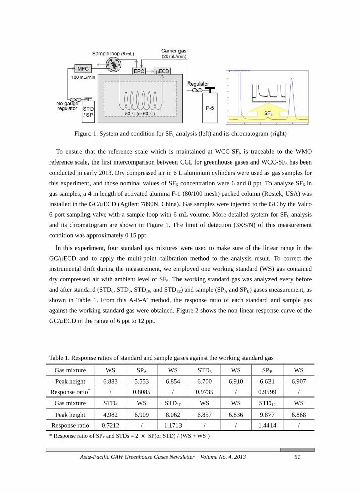
Asia-Pacific GAW Greenhouse Gases Newsletter Volume No. 4, 2013 51
Figure 1. System and condition for SF6 analysis (left) and its chromatogram (right)
To ensure that the reference scale which is maintained at WCC-SF6 is traceable to the WMO reference scale, the first intercomparison between CCL for greenhouse gases and WCC-SF6 has been conducted in early 2013. Dry compressed air in 6 L aluminum cylinders were used as gas samples for this experiment, and those nominal values of SF6 concentration were 6 and 8 ppt. To analyze SF6 in gas samples, a 4 m length of activated alumina F-1 (80/100 mesh) packed column (Restek, USA) was installed in the GC/μECD (Agilent 7890N, China). Gas samples were injected to the GC by the Valco 6-port sampling valve with a sample loop with 6 mL volume. More detailed system for SF6 analysis and its chromatogram are shown in Figure 1. The limit of detection (3 S/N) of this measurement condition was approximately 0.15 ppt.
In this experiment, four standard gas mixtures were used to make sure of the linear range in the GC/μECD and to apply the multi-point calibration method to the analysis result. To correct the instrumental drift during the measurement, we employed one working standard (WS) gas contained dry compressed air with ambient level of SF6. The working standard gas was analyzed every before and after standard (STD6, STD8, STD10, and STD12) and sample (SPA and SPB) gases measurement, as shown in Table 1. From this A-B-A’ method, the response ratio of each standard and sample gas against the working standard gas were obtained. Figure 2 shows the non-linear response curve of the GC/μECD in the range of 6 ppt to 12 ppt.
Table 1. Response ratios of standard and sample gases against the working standard gas
Gas mixture WS SPA WS STD8 WS SPB WS
Peak height 6.883 5.553 6.854 6.700 6.910 6.631 6.907
Response ratio* / 0.8085 / 0.9735 / 0.9599 /
Gas mixture STD6 WS STD10 WS WS STD12 WS
Peak height 4.982 6.909 8.062 6.857 6.836 9.877 6.868
Response ratio 0.7212 / 1.1713 / / 1.4414 / * Response ratio of SPs and STDs = 2 SP(or STD) / (WS + WS’)

52 Asia-Pacific GAW Greenhouse Gases Newsletter Volume No. 4, 2013
As shown in Figure 2, the GC/μECD used in WCC-SF6 has a non-linear response curve in the corresponding range. So it would be ideal to calibrate the GC using more than four standard gases at every measurement, but it consumed too much time and could be affected by unexpected instrumental drift during the measurement. Therefore, we would like to suggest the best calibration method by calculating the concentration of one sample (SPB) gas in difference calibration situations. SF6 concentration of sample B (SPB) which applies multi-point calibration (multi4p) using four standard gas mixtures was 7.854 ppt. This value was used as a reference value to compare each concentration value from various calibration situations. As shown in Table 2, as expected, any values calculated using STD8 showed good results. Single point calibrations using STD6 or STD10 were all valid as well. In some cases which apply single point calibration using STD12 and two point calibration using STD6 and STD12 showed big biases in the SPB measurement. Based on this result, the two-point calibration method was applied to this experiment to obtain accurate measurement results.
Table 3 shows the measurement result from WCC-SF6 for the intercomparison. Duplicate measurements by two-point calibration method (STD6 and STD8) were performed, and a multi-point calibration method (using four standard gases from 6 ppt to 12 ppt) was applied to only one result (the third measurement). As shown in the table, SF6 concentrations measured by WCC and CCL were agreed well within 0.034 ppt. This difference is slightly higher than the WMO recommended measurement target for SF6, but these two measured value were within their measurement uncertainty (standard deviation) each other.
Table 2. Calculated SF6 concentration of sample B from difference calibration situations (unit: ppt)
Single-point calibration
Standard gas STD6 STD8 STD10 STD12
SF6 concentration of SPB 7.879 7.861 7.863 7.916
Difference (Single-Multi4p) 0.025 0.007 0.009 0.062
Two-point calibration
Standard gas STD6, STD8 STD8, STD10 STD6, STD10 STD8, STD12
SF6 concentration of SPB 7.861 7.860 8.869 7.898
Difference (Two-Multi4p) 0.007 0.006 0.015 0.044
Three-point calibration
Standard gas STD6, STD8, and STD10 STD8, STD10, and STD12
SF6 concentration of SPB 7.861 7.862
Difference (Multi3p-Multi4p) 0.007 0.008
Figure 2. Response curve of GC used at WCC-SF6

Asia-Pacific GAW Greenhouse Gases Newsletter Volume No. 4, 2013 53
Table 3. Measurement result of two sample gases for the intercomparison (unit: ppt)
Sample Number of measurements WCC
[SD*] CCL [SD]
Difference (WCC-CCL)1 2 3 4 5
SPA 6.651 6.649 6.629 6.636 6.612 6.635
[0.016]6.633
[0.012] +0.002
SPB 7.841 7.833 7.851 7.828 7.901 7.851
[0.029]7.885
[0.019] -0.034
* SD: Standard Deviation
Based on these well established infrastructures and advanced measurement techniques for SF6,
WCC-SF6 will implement several long-term plans, such as to prepare operation procedures to maintain laboratory standard gases traceable to the WMO reference scale; to develop the measurement guideline for SF6 observation in cooperation with KRISS; to provide the technical training course for GAW stations to enhance their capability building for SF6 observation; to conduct intercomparison campaigns and system and performance audits for stations to improve the quality of observation data; and to expand the SF6 observation network including the in-situ and/or flask sampling analysis supported by several funding sources.
References [1] Singh HB et al. (1979). Atmospheric halocarbons, hydrocarbons, and sulfur hexafluoride: Global
distributions, sources, and sinks, Science, 203(4383). [2] WMO (2012) WMO Greenhouse Gas Bulletin No.8. ISSN 2078-0796 [3] Levin I et al. (2010). The global SF6 source inferred from long-term high precision atmospheric
measurements and its comparison with emission inventories, Atmos. Chem. Phys. 10. [4] Tollefson J (2010). Greenhouse-gas numbers up in the air, Nature, 465.


Asia-Pacific GAW Greenhouse Gases
Newsletter393-17 Haeangwangwang-ro Anmyeon-eup,
Taean-gun, Chungnam 357-961, Koreawww.climate.go.kr
Design by NAEDAM
l +82-31-421-8271


