CERN-THESIS-2015-139 27/01/2015 Scuola Dottorale in Scienze Matematiche e Fisiche XXVII Ciclo di Dottorato Associated production of the Higgs boson with a W boson in proton-proton collisions: an explorative analysis of the three-leptons final state with the ATLAS experiment Dottorando: Monica Trovatelli Docenti Guida: Prof. Filippo Ceradini Prof. Fabrizio Petrucci Coordinatore: Prof. Roberto Raimondi
Transcript
CER
N-T
HES
IS-2
015-
139
27/0
1/20
15
Scuola Dottorale in Scienze Matematiche e Fisiche
XXVII Ciclo di Dottorato
Associated production of the Higgs boson with a W boson in
proton-proton collisions: an explorative analysis of the
three-leptons final state with the ATLAS experiment
Dottorando:Monica Trovatelli
Docenti Guida:Prof. Filippo Ceradini
Prof. Fabrizio Petrucci
Coordinatore:Prof. Roberto Raimondi
Estuvo varios dıas como hechizado, repitiendose a sımismo en voz baja un sartal de asombrosasconjeturas, sin dar credito a su propioentendimiento. Por fin, un martes de diciembre, ala hora del almuerzo, solto de un golpe toda lacarga de su tormento. Los ninos habıan de recordarpor el resto de su vida la augusta solemnidad conque su padre se sento a la cabecera de la mesa,temblando de fiebre, devastado por la prolongadavigilia y por el encono de su imaginacion, y lesrevelo su descubrimiento:”La tierra es redonda como una naranja.”Ursula perdio la paciencia: ”Si has de volverte loco,vuelvete tu solo” grito. ”Pero no trates de inculcara los ninos tus ideas de gitano.”
GABRIEL GARCIA MARQUEZ,Cien anos de soledad (1967)
Acknowledgments
I would like to express my sincere gratitude to my advisor Professor Filippo Ceradini, for hiscontinuous support of my PhD research work; his guidance was for me extremely important andhis advices precious.
A special thanks goes to Professor Fabrizio Petrucci, who encouraged me during all theseyears and taught me how to pursue my own research approach. He was always patient as noone else, calming me down whenever anxious (and it doesn’t happen rarely!) and motivatingme when things became hard. I sincerely thank him for all the nights he spent to help me withmy research work, and for all the enjoyable (and often fruitful) coffee breaks we had together.
Thanks to my friend and colleague Marta, for sharing with me this experience and for joiningme in all the shopping afternoons.Thanks to Cecilia and Valerio (”Mr. simpatia”), for all the nice discussions we had and for thoseI hope we will have in the future.Thanks to Daniele, for always helping me when needed (and for having tried to teach me,unfortunately with no success, how to save money!), and thanks to Marco, a sincere friend I amglad to have met.Thanks to Monica, for having been my dear friend for so many years.
Thanks to Mauro, Michela, Paolo, Giuseppe, Domizia, Toni, Ada, Antonio and to all thefriends and colleagues in Rome for having made me feel part of a big family.
Of course thanks to Lorenzo, since he was (and incredibly still is!) able to stay and live withme. He is my confidant and my first supporter, thanks for enjoying with me my successes (butalso for comforting me for the defeats).
Last but not least, thanks to all my family, for having always believed this was possible,especially to my grandparents, for those who are still here and for those who are not anymore:thanks for being so proud of me, I am also proud of being your granddaughter!
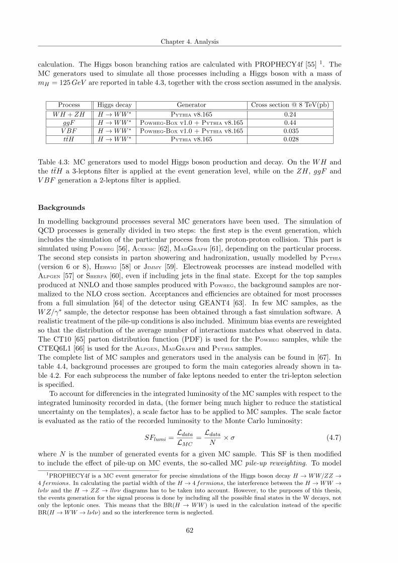
Since from the ancient era, man had the curiosity to know what we are made of, and looked foran explanation of everyday phenomena. Most of the questions found an answer in the early 20thcentury, when studies carried on by brilliant scientists gave birth to the Standard Model (SM) ofparticle physics. The SM is an elegant theory which explains, in a remarkable way, the structureof matter and the nature of fundamental interactions. In this theory particles divide in matterconstituents, the fermions, and particles which mediates the interactions between fermions, thebosons. Experiments carried on at the particle colliders, such as the LEP at the CERN laboratoryor the Tevatron at the Fermilab laboratory, have confirmed all the SM predictions with a highlevel of accuracy, also considering the wide energy range scanned. Hovewer, one important piecewas missing until its recent discovery at the Large Hadron Collider (LHC), the Higgs Boson,the particle responsible for the mass of the other SM particles, whose existence is postulatedin the Brout-Higgs-Englert (BEH) mechanism. On the 4th July 2012 the ATLAS and CMSexperiments at the CERN laboratory announced the observation of a new particle, with a massaround 125 GeV having, so far, all the characteristics of the Higgs boson. In 2013, the NobelPrize in Physics was awarded jointly to Peter Higgs and Francois Englert for their theoreticaldiscovery confirmed by the ATLAS and CMS experiments. The detailed studies of couplingsand properties of this new particle and the comparison with the expectations for the SM Higgsboson are the current focus of the ATLAS Collaboration. This thesis lies in this context, andpresents the work done by the author within the ATLAS Collaboration, aiming at studying theHiggs boson production and decay in the channel WH → WWW ∗ → lνlντν , (l = e/µ), usingthe proton-proton collision data collected in 2012.
The Higgs boson production in association with a vector boson offers the possibility tomeasure the coupling of the newly discovered particle with the W and Z bosons. These couplingsare predicted by the SM but have not been measured yet; in particular, the channel studied inthis thesis, with the Higgs boson further decaying in two W bosons, allows to direct probe theHiggs boson coupling exclusively with W bosons. The analysis here reported is an explorativestudy of the three leptons final state in the WH channel, one of the leptons being a hadronicallydecaying tau. The presence of a hadronic tau makes this channel challenging to study at theLHC, because of the high-jet activity at a hadron collider. However, the measure presentedis interesting as a feasibility study; the main issues of the measurement are addressed and thefundations for a similar study in LHC Run 2 are set.
This thesis is structured as follows. Chapter 1 introduces the Standard Model and the Brout-Englert-Higgs mechanism, the theory in which this study is embedded. Some recent resultsobtained by the ATLAS Collaboration about the measurements of spin, mass and couplings ofthe new particle are also reported. Chapter 2 gives an overview of the ATLAS detector, whichis the experimental apparatus used to collect data which this thesis is based on. In chapter 3 adescription of the lepton, jet and event identification and reconstruction techniques is presented.Chapter 4 presents the cut-based analysis done in the study of the WH → WWW ∗ → lνlντνprocess. A detailed description of the event selection using MC samples is reported, togetherwith the procedure used to normalize these MC samples to reproduce what observed in data.
9
Introduction
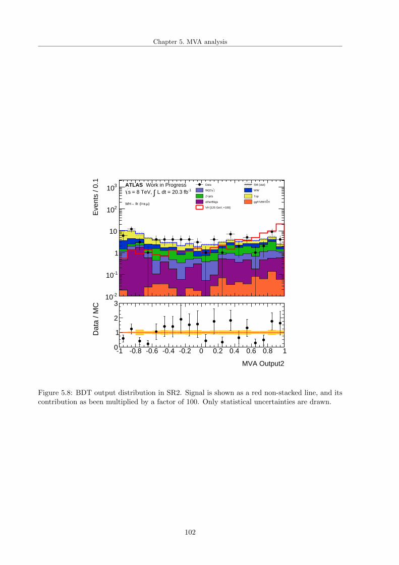
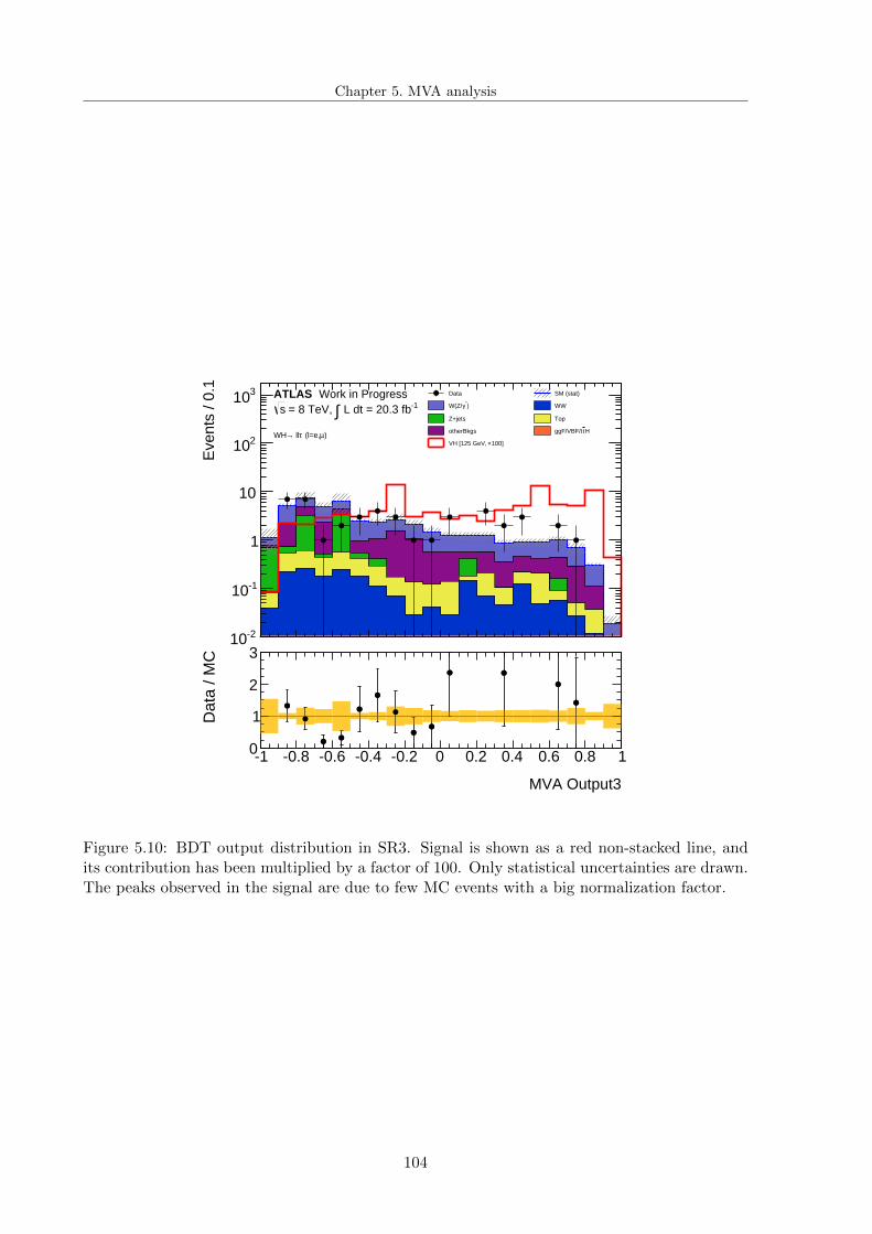
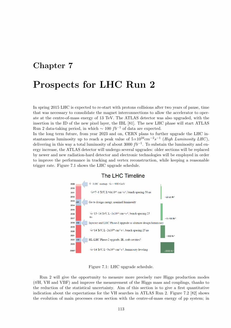
Due to the low sensitivity of the analysis, in chapter 5 an alternative approach to the cut-basedanalysis is presented: the multivariate analysis, aimed at reducing the background processes thatmimic the signal topology while keeping as much signal events as possible. Chapter 6 reportsand discusses the statistical analysis done to compare the results with the SM expectations.Finally in chapter 7 prospects for this measurement in LHC Run 2, when increased luminosityand centre-of-mass energy will be available, are given.
10
Chapter 1
Higgs boson discovery at LHC
The recent discovery of the Higgs boson at LHC (2012) was a big step towards the confirmation ofthe Standard Model as the theory that describes the sub-atomic particles and their interactions.In this chapter, after a brief review of the Standard Model theory, including the formulation ofthe simmetry breaking mechanism and the first attempts to search for the Higgs boson at theCERN electron-positron (LEP) and proton-antiproton (Tevatron) colliders, we will go throughthe main steps that led to the Higgs boson discovery.
1.1 The Standard Model
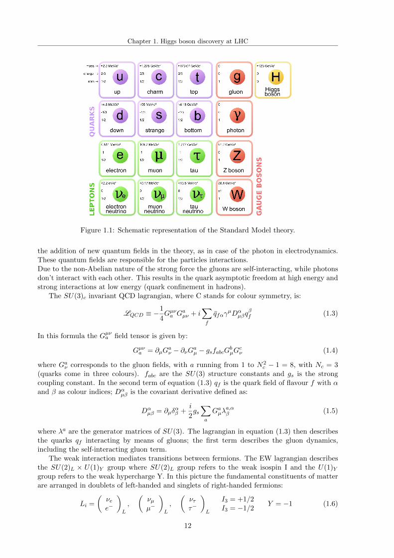
The Standard Model (SM) is the theory that accurately describes the elementary particles andtheir interactions as shown in the experiments. It is a renormalizable field theory that has beendeveloped during the 60’s thanks to the work of many people [1][2][3][4][5]. At the moment threeof the four forces observed in nature are described by the SM theory: the electromagnetism, theweak and the strong nuclear force. Any attempt to allocate the gravity in the SM has failed sofar. In the SM two type of point-like particles exist: fermions, spin-1/2 particles that are mattercontent, further divided in leptons and quarks, and the bosons, integer spin particles which arethe mediators of the interaction fields. Fermions interacts by the exchange of spin-1 bosons: eightmassless gluons and one massless photon for the strong and the electromagnetic interactions,respectively, and three massive bosons, W± and Z for the weak interaction. Fermions areorganized in a three-fold family structure, as shown in figure 1.1 which summarizes the currentknowledge of the sub-atomic world.
The SM is a non-Abelian Gauge theory based on the simmetry group SU(3)×SU(2)×U(1),where SU(3) is the non-Abelian gauge group of the Quantum Chromodynamics (QCD) [6],the theory describing the interaction of quarks and gluons due to colour charge, while theSU(2) × U(1) is the non-Abelian symmetry group of the combined electromagnetic and weakforces (electroweak). The SM lagrangian can then be written as:
LSM = LQCD + LEW (1.1)
It is invariant under a SU(3)×SU(2)×U(1) local gauge symmetry, where ”local” means that thetransformation depends on the specific space-time point x. Both the QCD and the EW theoriesare built by requiring a local invariance of the Dirac free lagrangian1 for the elementary matterfields, quarks in the first case, fermions in the second case. The local gauge invariance leads to
1The Dirac free lagrangian for a generic matter field Ψ is:
Lfree = Ψ(γµ∂µ −m)Ψ, Ψ ≡ Ψ+γ0 (1.2)
11
Chapter 1. Higgs boson discovery at LHC
Figure 1.1: Schematic representation of the Standard Model theory.
the addition of new quantum fields in the theory, as in case of the photon in electrodynamics.These quantum fields are responsible for the particles interactions.Due to the non-Abelian nature of the strong force the gluons are self-interacting, while photonsdon’t interact with each other. This results in the quark asymptotic freedom at high energy andstrong interactions at low energy (quark confinement in hadrons).
The SU(3)c invariant QCD lagrangian, where C stands for colour symmetry, is:
LQCD ≡ −1
4Gµνa Gaµν + i
∑f
qfαγµDα
µβqβf (1.3)
In this formula the Gµνa field tensor is given by:
Gµνa = ∂µGaν − ∂νGaµ − gsfabcGbµGcν (1.4)
where Gaν corresponds to the gluon fields, with a running from 1 to N2c − 1 = 8, with Nc = 3
(quarks come in three colours). fabc are the SU(3) structure constants and gs is the strongcoupling constant. In the second term of equation (1.3) qf is the quark field of flavour f with αand β as colour indices; Dα
µβ is the covariant derivative defined as:
Dαµβ = ∂µδ
αβ +
i
2gs∑a
Gaµλa,αβ (1.5)
where λa are the generator matrices of SU(3). The lagrangian in equation (1.3) then describesthe quarks qf interacting by means of gluons; the first term describes the gluon dynamics,including the self-interacting gluon term.
The weak interaction mediates transitions between fermions. The EW lagrangian describesthe SU(2)L × U(1)Y group where SU(2)L group refers to the weak isospin I and the U(1)Ygroup refers to the weak hypercharge Y. In this picture the fundamental constituents of matterare arranged in doublets of left-handed and singlets of right-handed fermions:
Li =
(νee−
)L
,
(νµµ−
)L
,
(νττ−
)L
I3 = +1/2I3 = −1/2
Y = −1 (1.6)
12
Chapter 1. Higgs boson discovery at LHC
Qi =
(ud
)L
,
(cs
)L
,
(tb
)L
I3 = +1/2I3 = −1/2
Y = +1/3 (1.7)
lR,i = e−R , µ−R , τ−R , I3 = 0 Y = −1 (1.8)
uR,i = uR , cR , tR , I3 = 0 Y = −4/3 (1.9)
dR,i = dR , sR , bR , I3 = 0 Y = −2/3 (1.10)
In the above equations I3 is the third component of the weak isospin. The weak ipercharge isrelated to the weak isospin through the following equation:
Y = 2
(Q
e− I3
)(1.11)
The request of the local gauge invariance leads to the introduction of four vector bosons: theW i fields (i=1,2,3) for the SU(2)L group and the field B for the U(1)Y group. The physicalfields Aµ (photon field), Zµ (the field associated to the neutral boson Z0) and W± (the fieldsdescribing the two charged bosons) can be obtained by a combination of the gauge fields:
Aµ = Bµ cos θW +W 3µ sin θW (1.12)
Zµ = W 3µ cos θW −Bµ sin θW (1.13)
W±µ =W 1µ ∓ iW 2
µ√2
(1.14)
In the above equations the angle θW , which specifies the mixture of Zµ and Aµ fields in W 3µ and
Bµ is known as the mixing angle. The weak mixing angle θW also relates the masses of the weakbosons, as shown in section 1.2.The analytic form of the EW lagrangian is:
LEW = −1
4
∑G
FµνG Fµν G + i∑f
fDµγµf (1.15)
where the index G indicates that the first sum in equation (1.15) is extended to all the vectorialfields, while the index f indicates that the second sum is extended to all the fermionic fields. Thefirst term in equation (1.15) describes the dynamics of the bosons, while the second term theinteraction between fermions, interaction that is mediated by the four bosons. The interactionbetween fermions and bosons can be derived by writing down the definition of the covariantderivative:
Dµ = ∂µ − igG(λαGα)µ (1.16)
where gG is the coupling constant to the G field (G = A, Z, W± and λα are the generators ofthe group to which the G field refers (SU(2) or U(1))).
The SM lagrangian as written above is gauge invariant but it doesn’t contain any mass termfor fermions and bosons. This contradicts the experimental evidence that, apart for the photon,the particles that we observe have a non-zero mass. Any attempt to include ad-hoc mass termsin the lagrangian spoils the gauge invariance and the renormalizability of the theory. In the mid-1960 a couple of different works carried on by several theoreticians ([7][8][9][10]) tried to explainthe origin of particle masses; these works showed how the gauge invariance of the lagrangiancan be preserved by invoking the spontaneous EW lagrangian symmetry breaking (also knownas the Brout-Englert-Higgs (BEH) mechanism).
13
Chapter 1. Higgs boson discovery at LHC
1.2 The Brout-Englert-Higgs mechanism
The BEH mechanism is the generalization of the Goldstone model (details can be found in [11])to the case of a lagrangian invariant for a local phase trasformation. In this mechanism theassumption is made that everywhere in space, fluctuations in the vacuum can occur whichcorrespond to the emission or the absorption of a Higgs boson, a spin 0, electrically neutralparticle with no colour charge. As a result of their interactions with the Higgs field, the W± andZ0 bosons and the fermions acquire mass, but gluons and photons remain massless. The choice ofa specific vacuum state results in the spontaneous symmetry breaking of the local SU(2)×U(1)gauge symmetry and gives rise to the spectrum of particles we observe. Spontaneous symmetrybreaking is relevant in a field theory only if the ground state is not-unique. In the following theBEH mechanism is briefly derived starting from the Goldstone model; a detailed description canbe found in [7][8][9][10].
The simplest example of a field theory exhibiting the spontaneous symmetry breaking is theGoldstone model. The Goldstone model is the model of a real scalar field φ with a lagrangiangiven by
L =1
2(∂µφ)(∂µφ)− V (φ) (1.17)
withV (φ) = µ2φ2 + λφ4 (1.18)
λ and µ2 are arbitrary real parameters. The first term in equation (1.17) is positive defined andvanishes for constant φ. It follows that the minimum of the total energy of the field correspondsto the minimum of the potential V (φ). To guarantee the existence of a ground state for sucha potential λ > 0 is also requested. For positive values of µ2, the minimum of the potential isat φ = 0. However another situation can occur, in case µ2 < 0 the potential possesses a localminimum at φ(x) = 0 and a whole circle of absolute minimum at
φ(x) = φ0 =
(−µ2
2λ
)1/2
eiθ (1.19)
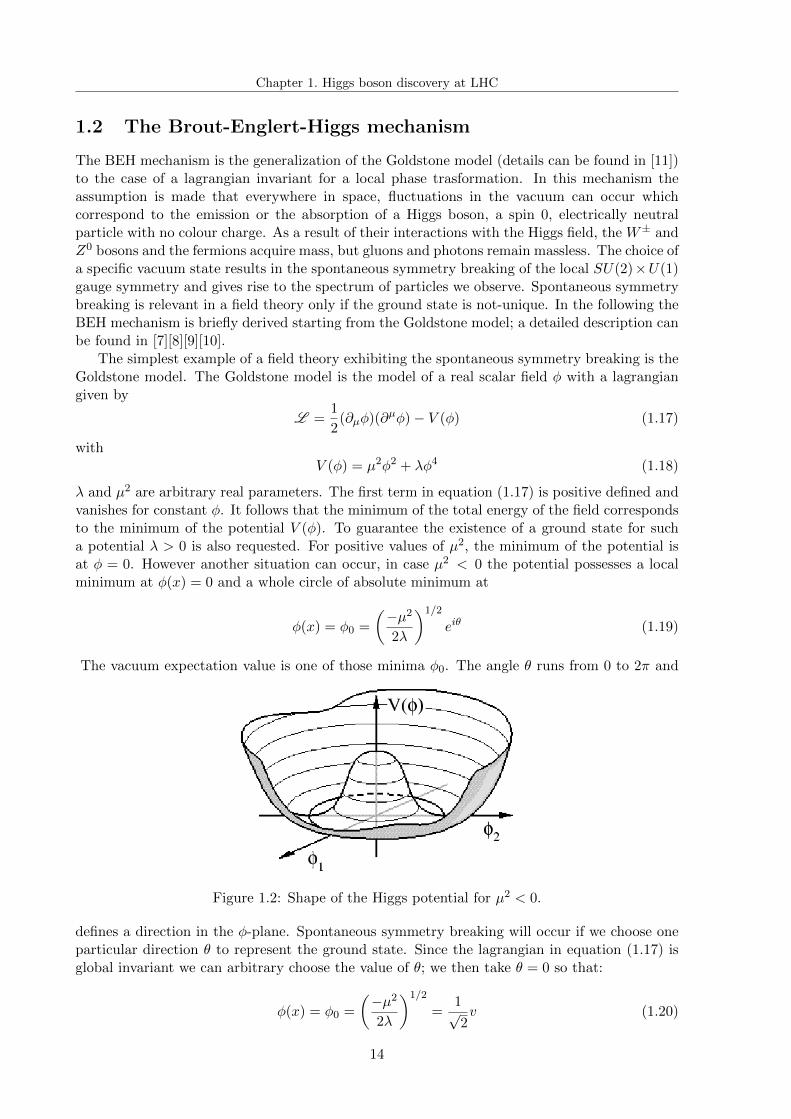
The vacuum expectation value is one of those minima φ0. The angle θ runs from 0 to 2π and
Figure 1.2: Shape of the Higgs potential for µ2 < 0.
defines a direction in the φ-plane. Spontaneous symmetry breaking will occur if we choose oneparticular direction θ to represent the ground state. Since the lagrangian in equation (1.17) isglobal invariant we can arbitrary choose the value of θ; we then take θ = 0 so that:
φ(x) = φ0 =
(−µ2
2λ
)1/2
=1√2v (1.20)
14
Chapter 1. Higgs boson discovery at LHC
is real.This is how the spontaneous symmetry breaking occurs. In the following we will show how thisconcept can be applied to the SM and how the spontaneous breaking can generate the massesof bosons and fermions.
The simplest way to introduce the spontaneous symmetry breaking in the SM lagrangian isby adding a new SU(2)L doublet of complex scalar field (called the Higgs field):
Φ =
(φ+
φ0
)(1.21)
The lagrangian of this scalar doublet is
LH = (DµΦ)†(DµΦ)− µ2Φ†Φ− λ(Φ†Φ)2 (1.22)
where the covariant derivative is
Dµ = ∂µ +i
2gτjW
µj +
1
2g′Y Bµ (1.23)
where the sum over the index j = 1,2,3 is implied, τj are the Pauli matrices, g and g’ are thecoupling constants of fermions to the Wµ and Bµ respectively and Y is the weak hyperchargeoperator. This lagrangian contains the symmetric potential in figure 1.2, which has again avacuum expectation value different from zero, which can be choosen to be
Φ0 =
(0
v/√
2
)(1.24)
where v = (−µ2/λ)1/2. Equation (1.24) states that the ground state of the V (Φ) potential occursfor a non-vanishing value of the Φ field. The ground state is not symmetric under SU(2)L×U(1)Ytransformation since there is a preferred direction, and the symmetry is spontaneously broken.To understand the physical content of this mechanism we expand the lagrangian perturbativelyaround its ground state. In general we can express the Φ field around the ground state as
Φ =1√2
(0
v + σ(x)
)(1.25)
The gauge in which the Higgs field has the above form is called the unitary gauge. In this gaugethe imaginary part of the complex Φ field can be eliminated through a local transformation ofthe field. The Φ field has then become real. By substituting the expansed expression for theHiggs field in the lagrangian in equation (1.22) we find
L =1
2∂µσ∂
µσ + 2µ2σ2 − 2√−2λµ2σ3 − λσ4 + const. (1.26)
The real field σ(x) measures the deviation of the field Φ(x) from the equilibrium ground stateconfiguration Φ(x) = Φ0. Equation (1.26) can be interpreted as the lagrangian of a scalar fieldσ(x) with mass
√2λv2. The equation includes a cubic term that breaks the symmetry of the
potential in picture 1.2 (the potential is anymore invariant under the transformation x→ −x).The Higgs field Φ(x) describes a scalar neutral particle, the Higgs boson, of mass
mH =√
2µ =√
2λv (1.27)
The value of mH depends on µ and it is a free paremeter of the SM.
15
Chapter 1. Higgs boson discovery at LHC
1.2.1 Bosons masses
Bosons masses originate from the interaction of the SU(2)×U(1) gauge fields (Wµ and Zµ) withthe Higgs field. This interaction takes place through the covariant derivative Dµ in equation(1.23). Substituting the covariant derivative in the scalar lagrangian of equation (1.22) one getsfor the kinetic term:
(DµΦ)†DµΦ→ 1
2∂µσ∂
µσ + (v + σ)2
(g2
4W †µW
µ +g2
8 cos2 θWZµZ
µ
)(1.28)
Both the W± and the Z0 bosons have acquired mass, since they appear in the previous formulaas quadratic terms. The mass of the W± and the Z0 bosons are related through the equation:
MZ cos θW = MW =1
2vg (1.29)
and given that
tan θ =g′
g(1.30)
we can also writeMW =
vg
2(1.31)
MZ =v
2
√g2 + g′2 (1.32)
1.2.2 Fermions masses
Fermions masses are generated by coupling the Higgs doublet and the fermions. The additionalYukawa term to add at the SM lagrangian has the form
L = −gψ(ψLΦψR) + h.c. (1.33)
where gψ is the coupling constant of the fermionic field ψ to the Higgs field. ψL and ψR are theleft- and right-handed fermion fields respectively. Expanding again equation (1.33) around theground state of the Higgs field we can derive the fermion mass term:
mψ = gψv/√
2 (1.34)
From equations (1.29) and (1.34) it is possible to note that bosons and fermions massesstrongly depend on the value of the parameter v, as well as on the mH . It can be shown [12]that the parameter v is related to the Fermi constant GF through
v = (√
2GF )−1/2 ≈ 246GeV (1.35)
This in the past allowed to predict the mass of the W± bosons and the mass of the Z0 boson,before they were discovered at the UA1 and UA2 experiments. In the SM framework the Higgsboson self-coupling parameter λ is then the only free parameter of the theory; because of theequation (1.27) also the Higgs boson mass value was unknown until its discovery at LHC. Asshown in the next section, the Higgs boson production and decay modes depend on its mass;for this reason some decades ago people started to look for the Higgs in the various productionand decay channels, since each mode was in principle possibile and accessible at a given energy.
1.3 The Higgs boson at the LHC
Decades after the Higgs theory was established, the Higgs boson was discovered in 2012 by theATLAS and CMS collaborations [13][14]. In this section production and decays modes of theHiggs boson at a hadron collider are discussed.
16
Chapter 1. Higgs boson discovery at LHC
1.3.1 Production
As shown in the previous section, the Higgs boson couples to bosons and fermions with differentcouplings; in particular the coupling with fermions is proportional to the mass of the fermion,while the coupling with the bosons is proportional to the square mass of the boson. The Higgs-fermions coupling gHff =
mfv is of the order of mf/mW , and it is weak for mf << mW ;
this condition is satisfied for neutrinos, electrons, muons and the light quarks (u,d,s). Hence,although is in principle possible for the Higgs boson to be produced by these particles, the
production cross sections are very small. The value of the Higgs-boson coupling gHV V =2m2
Vv ,
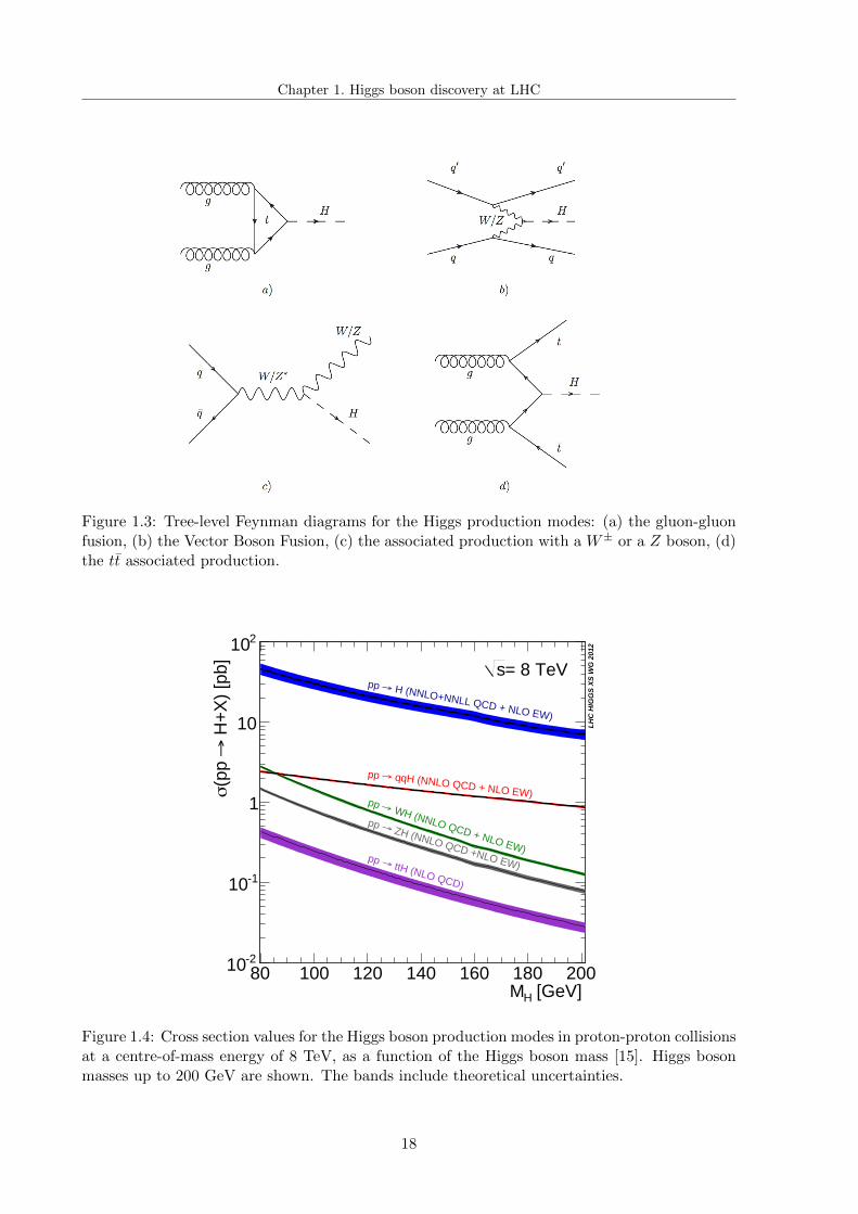
being proportional to the square mass of the boson V which the Higgs boson couples to, makesthis production mode more probable, thanks to the fact that these bosons are very massive withrespect to fermions. The four main Higgs production modes are summariezed in figure 1.3. Theirrelative importance depends on the centre-of-mass energy; at LHC running with a centre-of-massenergy of 8 TeV they are, from the most to the least probable:
Gluon-gluon fusion (ggF): it is the dominant Higgs boson production mode. Two gluonsfrom the colliding protons couple to the Higgs boson through a fermion loop; because oftheir mass, top quarks are the most probable to contribute to the loop. This productionchannel has no distinctive experimental signature; it can be detected only with a clearidentification of the Higgs boson decay products.
Vector boson fusion (VBF): it is the second Higgs boson production mode at the LHC,with a cross section a factor 10 smaller than the ggF. Two quarks from the collidingprotons emit two virtual bosons V, which in turn fuse to produce the Higgs boson. Theprocess is characterized by the emission of two high− pT jets, called tagging jets, directedpredominantly in the forward region.
Associated production with a vector boson (VH, V=W/Z): it is known as the Higgs-strahlung process. In fact it consists in a quark-antiquark annihilation to create a vectorboson V, with V=W/Z, which then radiates an Higgs boson. Although the cross sectionfor this process is low compared to the ggF and VBF processes, it gives the chance todirectly test the coupling of the Higgs boson with a vector boson, and so to test the SMpredictions.A study of the WH associated production in final states with three leptons, one being atau, is the subject of this thesis. For this reason the last paragraph of this chapter willcontain a brief review of the VH process at hadron colliders.
Associated production with heavy quarks (ttH): it is the least probable Higgs bosonproduction mode at the LHC. The initial state gluons exchange a top quark from whicha Higgs boson is produced. This process offers the possibility to measure the top Yukawacoupling. Even though the latter is large, thanks to the high mass of the top quark, theheavy ttH final state is kinematically suppressed. The cross section results to be a factor100 smaller than ggF cross section.
In figure 1.4 the cross section values for the production modes listed above are shown asa function of the Higgs boson mass. The exact values, for a centre-of-mass energy of 8 TeVand for the measured value of the Higgs boson mass mH = 125 GeV, are reported in table 1.1and compared with the 13 TeV values, 13 TeV being the centre-of-mass energy expected in thesecond data-taking run of LHC (Run 2). Run 2 starting date is scheduled for March 2015.
17
Chapter 1. Higgs boson discovery at LHC
Figure 1.3: Tree-level Feynman diagrams for the Higgs production modes: (a) the gluon-gluonfusion, (b) the Vector Boson Fusion, (c) the associated production with a W± or a Z boson, (d)the tt associated production.
[GeV] HM80 100 120 140 160 180 200
H+
X)
[pb]
→(p
p σ
-210
-110
1
10
210= 8 TeVs
LH
C H
IGG
S X
S W
G 2
012
H (NNLO+NNLL QCD + NLO EW)
→pp
qqH (NNLO QCD + NLO EW)
→pp
WH (NNLO QCD + NLO EW)
→pp
ZH (NNLO QCD +NLO EW)
→pp
ttH (NLO QCD)
→pp
Figure 1.4: Cross section values for the Higgs boson production modes in proton-proton collisionsat a centre-of-mass energy of 8 TeV, as a function of the Higgs boson mass [15]. Higgs bosonmasses up to 200 GeV are shown. The bands include theoretical uncertainties.
18
Chapter 1. Higgs boson discovery at LHC
Higgs production cross sections in pb at LHC for mH = 125 GeV√s ggF VBF WH ZH ttH
8 TeV 19.3+10%−10% 1.6+3%
−3% 0.7+3%−3% 0.4+4%
−4% 0.1+9%−12%
13 TeV 44.0+10%−10% 3.8+5%
−5% 1.4+3%−4% 0.9+4%
−4% 0.5+11%−13%
Table 1.1: Cross section values (in pb) for the main Higgs production modes at LHC, for acentre-of-mass energy of 8 TeV and 13 TeV. All the cross section values, except for the ttH, arecomputed at NNLO in perturbation theory for the QCD corrections [16][17][18], and at NLOfor the EW corrections. The ttH cross-section which is computed at NLO in QCD. The quoteduncertainty has been computed by adding in quadrature the error obtained by varying the QCDscale and that obtained by varying the PDF set.
1.3.2 Decay
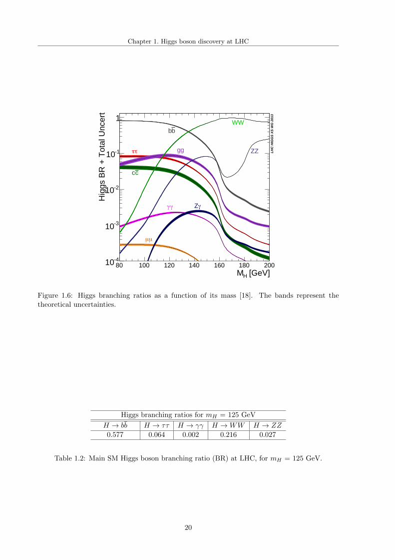
Since the couplings of the Higgs boson are proportional to masses, as mH increases the Higgsparticle becomes strongly coupled. This reflects in the sharp rise of the Higgs boson total width,shown in figure 1.5 as a function of the Higgs mass. In figure 1.6 the Higgs boson branchingratios are shown; the values for mH = 125 GeV are reported in table 1.2.
[GeV]HM
100 200 300 1000
[GeV
]H
Γ
-210
-110
1
10
210
310
LH
C H
IGG
S X
S W
G 2
010
500
Figure 1.5: Higgs total width as a function of its mass [16].
Two Higgs boson mass region can be distinguished, the low mass region for mH . 135 GeV,and the high mass region, for mH > 135 GeV. In the low mass region the dominant decay modeis the H → bb, which is hard to be identified at LHC because of the high multi-jets background.The H → γγ proceeds via a W loop; despite the branching ratio of this process is very lowcompared to the bb mode, the clean signature of two photons made this channel one of the
19
Chapter 1. Higgs boson discovery at LHC
[GeV]HM80 100 120 140 160 180 200
Hig
gs B
R +
Tot
al U
ncer
t
-410
-310
-210
-110
1
LH
C H
IGG
S X
S W
G 2
013
bb
ττ
µµ
cc
gg
γγ γZ
WW
ZZ
Figure 1.6: Higgs branching ratios as a function of its mass [18]. The bands represent thetheoretical uncertainties.
Higgs branching ratios for mH = 125 GeV
H → bb H → ττ H → γγ H →WW H → ZZ
0.577 0.064 0.002 0.216 0.027
Table 1.2: Main SM Higgs boson branching ratio (BR) at LHC, for mH = 125 GeV.
20
Chapter 1. Higgs boson discovery at LHC
preferred for its discovery at LHC. The width sharply increases as soon as the WW threshold isapproached. Below this threshold the decays into off-shell V particles is important, for examplethe H → WW ∗ decay. The dip of the ZZ branching ratio just below the ZZ threshold, inparticular, is due to the fact that the W boson is lighter than the Z boson, and the opening ofits threshold depletes all the other banching ratios. For mH > 160 GeV both the H → WWand the H → ZZ modes are possibile. These two channels had a leading role in the Higgsboson discovery (see section 1.3.3); leptonic vector boson decays were selected, which allowed todecrease the background contribution while keeping high the acceptance on the signal events.
1.3.3 The Higgs boson discovery
The Higgs boson has been the subject of many physics searches in the last decades at particlecolliders. Before the advent of LHC, direct searches for the Higgs boson were carried on atthe Large Electron-Positron collider (LEP), first, and then at the Tevatron proton-antiprotoncollider. A lower bound on the Higgs boson mass of 114.4 GeV at 95% CL has been set withLEP [19] data, while Tevatron studies reported an excess of events around mH = 125 GeV witha significance of 3.0σ [20], mainly from searches in the V H → V bb channel.
The search for the Higgs boson culminated in its discovery on the 4th July 2012, whenboth ATLAS and CMS Collaborations reported an excess of events in the region 124-126 GeV,compatible with the existence of a SM Higgs boson of that mass. The significance of the excessobtained by combining the 8 TeV result with the previous 7 TeV result, was 4.9 and 5.0 standarddeviations respectively, which in both cases is enough to claim the discovery of an Higgs-bosonlike particle [13][14]. In this section only ATLAS published results on the Higgs search anddiscovery are discussed.
The observation of the SM Higgs boson was possible thanks to the combination of theindividual searches, carried on in the H → γγ, H → ZZ(∗) → 4l and H → WW (∗) → lνlνchannels. In november 2013 also the evidence for the decays into fermions was obtained in theH → ττ and H → bb channels [21][22].
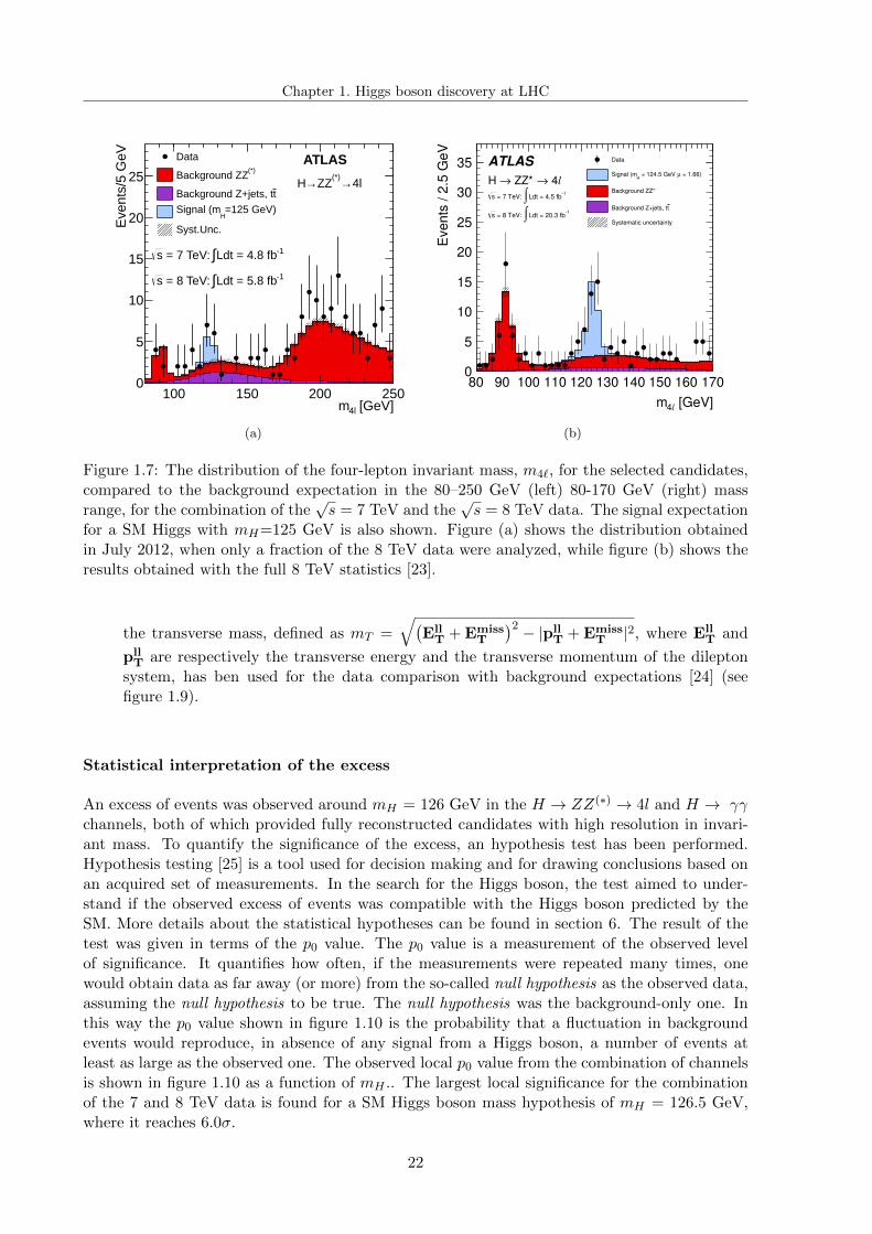
Four leptons: The H → ZZ(∗) → 4l channel, where l = e, µ, is also called the ”golden-channel” for the Higgs boson discovery at LHC, since it has a clean signature and very smallbackground contribution, even if it is characterized by a tiny cross section. It provides goodsensitivity over a wide mass range (110-600 GeV), largely due to the excellent momentumresolution of the ATLAS detector (see chapter 2). The selection of four charged leptonsin the final state allows to fully reconstruct the Higgs boson invariant mass. Data arecompared with the expected distribution of the four leptons invariant mass m4l for thebackground and for a Higgs boson signal with mH = 125 GeV [23]; the result is shown infigure 1.7.
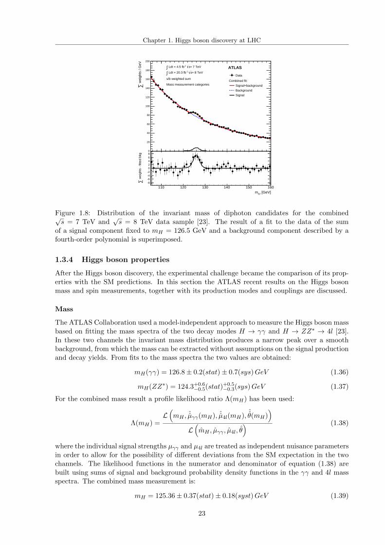
Two photons: Thanks to the excellent di-photon invariant mass resolution, the H → γγchannel was one of the most important channels for the Higgs discovery at LHC. In fact itwas possible to distinguish the peak due to the tiny expected signal over the huge diphotonbackground with a smooth distribution. The result obtained with the combination of the√s = 7 TeV and the
√s = 8 TeV data is shown in figure 1.8. An excess of events around
mH = 126.5 GeV was observed [23].
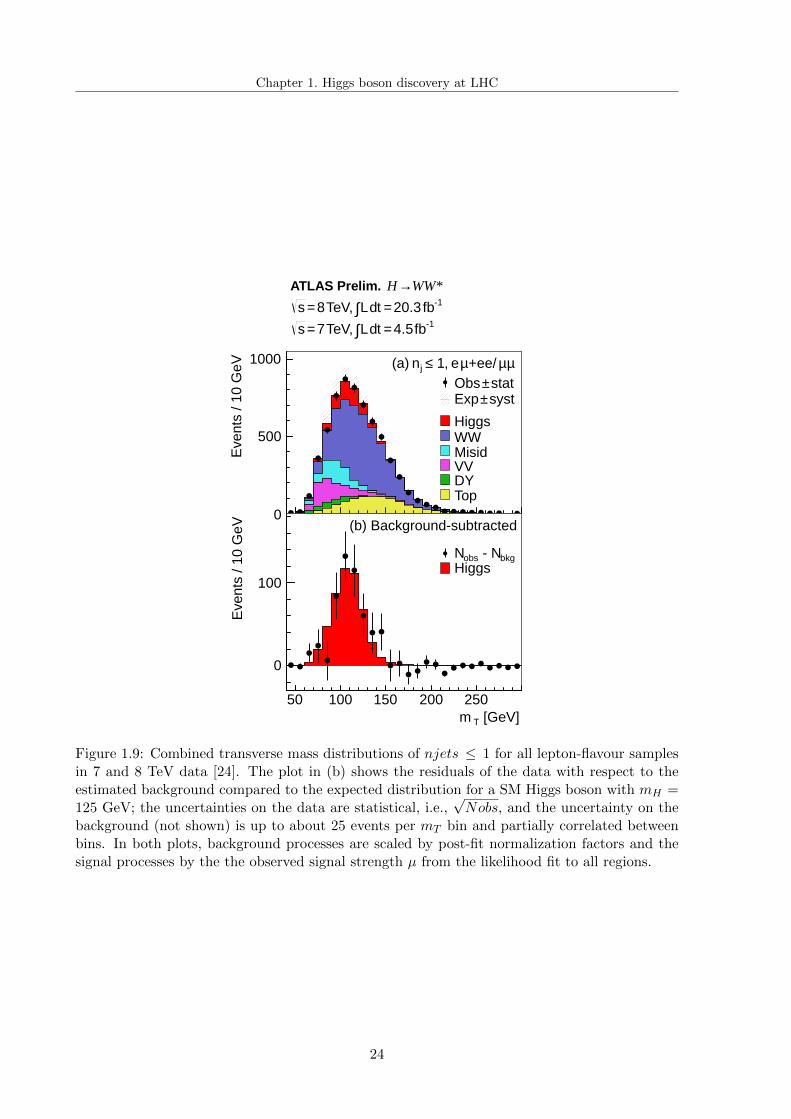
WW channel: The process H → WW (∗) → lνlν is highly sensitive to a SM Higgs bosonin the mass range around the WW threshold of 160 GeV. The signature for this channelis two opposite charge leptons with large transverse momentum and a large momentumimbalance in the event due to the escaping neutrinos. The presence of neutrinos in thefinal state doesn’t allow the reconstruction of the Higgs invariant mass. For this reason
21
Chapter 1. Higgs boson discovery at LHC
[GeV]4lm100 150 200 250
Eve
nts/
5 G
eV
0
5
10
15
20
25
-1Ldt = 4.8 fb∫ = 7 TeV: s
-1Ldt = 5.8 fb∫ = 8 TeV: s
4l→(*)ZZ→H
Data(*)Background ZZ
tBackground Z+jets, t
=125 GeV)H
Signal (m
Syst.Unc.
ATLAS
(a)
[GeV]l4m
80 90 100 110 120 130 140 150 160 170
Eve
nts
/ 2
.5 G
eV
0
5
10
15
20
25
30
35 Data
= 1.66)µ = 124.5 GeV H
Signal (m
Background ZZ*
tBackground Z+jets, t
Systematic uncertainty
l 4→ ZZ* →H 1
Ldt = 4.5 fb∫ = 7 TeV: s
1Ldt = 20.3 fb∫ = 8 TeV: s
ATLAS
(b)
Figure 1.7: The distribution of the four-lepton invariant mass, m4`, for the selected candidates,compared to the background expectation in the 80–250 GeV (left) 80-170 GeV (right) massrange, for the combination of the
√s = 7 TeV and the
√s = 8 TeV data. The signal expectation
for a SM Higgs with mH=125 GeV is also shown. Figure (a) shows the distribution obtainedin July 2012, when only a fraction of the 8 TeV data were analyzed, while figure (b) shows theresults obtained with the full 8 TeV statistics [23].
the transverse mass, defined as mT =√(
EllT + Emiss
T
)2 − |pllT + Emiss
T |2, where EllT and
pllT are respectively the transverse energy and the transverse momentum of the dilepton
system, has ben used for the data comparison with background expectations [24] (seefigure 1.9).
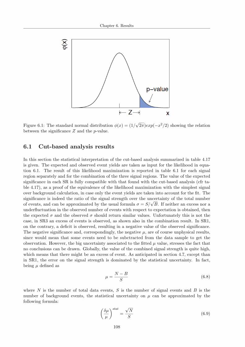
Statistical interpretation of the excess
An excess of events was observed around mH = 126 GeV in the H → ZZ(∗) → 4l and H → γγchannels, both of which provided fully reconstructed candidates with high resolution in invari-ant mass. To quantify the significance of the excess, an hypothesis test has been performed.Hypothesis testing [25] is a tool used for decision making and for drawing conclusions based onan acquired set of measurements. In the search for the Higgs boson, the test aimed to under-stand if the observed excess of events was compatible with the Higgs boson predicted by theSM. More details about the statistical hypotheses can be found in section 6. The result of thetest was given in terms of the p0 value. The p0 value is a measurement of the observed levelof significance. It quantifies how often, if the measurements were repeated many times, onewould obtain data as far away (or more) from the so-called null hypothesis as the observed data,assuming the null hypothesis to be true. The null hypothesis was the background-only one. Inthis way the p0 value shown in figure 1.10 is the probability that a fluctuation in backgroundevents would reproduce, in absence of any signal from a Higgs boson, a number of events atleast as large as the observed one. The observed local p0 value from the combination of channelsis shown in figure 1.10 as a function of mH .. The largest local significance for the combinationof the 7 and 8 TeV data is found for a SM Higgs boson mass hypothesis of mH = 126.5 GeV,where it reaches 6.0σ.
Figure 1.8: Distribution of the invariant mass of diphoton candidates for the combined√s = 7 TeV and
√s = 8 TeV data sample [23]. The result of a fit to the data of the sum
of a signal component fixed to mH = 126.5 GeV and a background component described by afourth-order polynomial is superimposed.
1.3.4 Higgs boson properties
After the Higgs boson discovery, the experimental challenge became the comparison of its prop-erties with the SM predictions. In this section the ATLAS recent results on the Higgs bosonmass and spin measurements, together with its production modes and couplings are discussed.
Mass
The ATLAS Collaboration used a model-independent approach to measure the Higgs boson massbased on fitting the mass spectra of the two decay modes H → γγ and H → ZZ∗ → 4l [23].In these two channels the invariant mass distribution produces a narrow peak over a smoothbackground, from which the mass can be extracted without assumptions on the signal productionand decay yields. From fits to the mass spectra the two values are obtained:
mH(γγ) = 126.8± 0.2(stat)± 0.7(sys)GeV (1.36)
mH(ZZ∗) = 124.3+0.6−0.5(stat)+0.5
−0.3(sys)GeV (1.37)
For the combined mass result a profile likelihood ratio Λ(mH) has been used:
Λ(mH) =L(mH , ˆµγγ(mH), ˆµ4l(mH),
ˆθ(mH)
)L(mH , µγγ , µ4l, θ
) (1.38)
where the individual signal strengths µγγ and µ4l are treated as independent nuisance parametersin order to allow for the possibility of different deviations from the SM expectation in the twochannels. The likelihood functions in the numerator and denominator of equation (1.38) arebuilt using sums of signal and background probability density functions in the γγ and 4l massspectra. The combined mass measurement is:
mH = 125.36± 0.37(stat)± 0.18(syst)GeV (1.39)
23
Chapter 1. Higgs boson discovery at LHC
Eve
nts
/ 10
GeV
500
1000
50 100 150 200 250 300
Eve
nts
/ 10
GeV
0
100
0
stat ± Obssyst ± Exp
HiggsWWMisidVVDYTop
bkg - NobsNHiggs
(b) Background-subtracted
[GeV]Tm
µµee/+µe, 1≤jn(a)
ATLAS Prelim. WW*→H-1fb 20.3 = td L∫TeV, 8 = s
-1fb 4.5 = td L∫TeV, 7 = s
Figure 1.9: Combined transverse mass distributions of njets ≤ 1 for all lepton-flavour samplesin 7 and 8 TeV data [24]. The plot in (b) shows the residuals of the data with respect to theestimated background compared to the expected distribution for a SM Higgs boson with mH =125 GeV; the uncertainties on the data are statistical, i.e.,
√Nobs, and the uncertainty on the
background (not shown) is up to about 25 events per mT bin and partially correlated betweenbins. In both plots, background processes are scaled by post-fit normalization factors and thesignal processes by the the observed signal strength µ from the likelihood fit to all regions.
24
Chapter 1. Higgs boson discovery at LHC
[GeV]Hm110 115 120 125 130 135 140 145 150
0Lo
cal p
-1110
-1010
-910
-810
-710
-610
-510
-410
-310
-210
-110
1
Obs. Exp.
σ1 ±-1Ldt = 5.8-5.9 fb∫ = 8 TeV: s
-1Ldt = 4.6-4.8 fb∫ = 7 TeV: s
ATLAS 2011 - 2012
σ0σ1σ2
σ3
σ4
σ5
σ6
Figure 1.10: The observed (solid) local p0 as a function of mH in the low mass range [13]. Thedashed curve shows the expected local p0 under the hypothesis of a SM Higgs boson signal atthat mass with its plus/minus one sigma band. The horizontal dashed lines indicate the p-valuescorresponding to significances of 1 to 6 sigma.
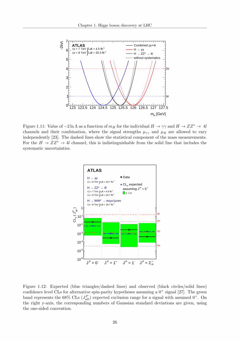
The −2 ln Λ value as a function of mH for the individual H → γγ and H → ZZ∗ → 4l channelsand their combination is shown in figure 1.11. In order to assess the compatibility of the massmeasurements from the two channels a dedicated test statistic has been used. From the valueof −2 ln Λ at ∆mH = 0, a compatibility of 4.8%, equivalent to 1.98σ, is estimated.
Spin
In the SM, the Higgs boson is a spin-0 and CP-even particle (JP = 0+). The spin-parity of theobserved Higgs boson has been evaluated independently in the H → γγ, H → ZZ∗ → 4l andH → WW ∗ → lνlν channels; the results have then been combined and the spin obtained. Theanalysis in each channel relies on discriminant observables chosen to be sensitive to the spin andthe parity of the signal. Several spin-parity hypothesis have been tested: JP = 0+, 0−, 1+, 1−, 2+.A likelihood function L(JP , µ, θ) is built for each spin-parity assumption and a test statistic qused to distinguish between two signal spin-parity hypothesis at a time is performed, based ona ratio of likelihoods:
q = logL(JP = 0+, ˆµ0+ ,
ˆθ0+
)L(JPalt,
ˆµJPalt,ˆθJPalt
) (1.40)
where JPalt is the alternative hypothesis to be tested. Variables sensitive to the Higgs spin-parityare for example the dilepton invariant mass mll and the azimuthal separation of the two leptons,∆φll, in the H →WW ∗ → lνlν event topologies. The data favour the SM quantum numbers ofJP = 0+ [27], while the other hypotheses are rejected. Results are shown in figure 1.12.
Production and couplings
The Higgs boson production strength, the parameter µ, has been determined from a fit to datausing the profile likelihood ratio Λ(µ) for a fixed mass hypothesis corresponding to the measuredvalue. The overall signal production strength is measured to be:
µ = 1.33± 0.14(stat)± 0.15(sys) (1.41)
25
Chapter 1. Higgs boson discovery at LHC
[GeV]Hm
123 123.5 124 124.5 125 125.5 126 126.5 127 127.5
Λ-2
ln
0
1
2
3
4
5
6
7
σ1
σ2
ATLAS-1Ldt = 4.5 fb∫ = 7 TeV s
-1Ldt = 20.3 fb∫ = 8 TeV s
l+4γγCombined γγ →H
l 4→ ZZ* →H without systematics
Figure 1.11: Value of −2 ln Λ as a function of mH for the individual H → γγ and H → ZZ∗ → 4lchannels and their combination, where the signal strengths µγγ and µ4l are allowed to varyindependently [23]. The dashed lines show the statistical component of the mass measurements.For the H → ZZ∗ → 4l channel, this is indistinguishable from the solid line that includes thesystematic uncertainties.
- = 0 PJ + = 1 PJ - = 1 PJ m + = 2 PJ
ATLAS
4l→ ZZ* →H -1Ldt = 4.6 fb∫ = 7 TeV s
-1Ldt = 20.7 fb∫ = 8 TeV s
γγ →H -1Ldt = 20.7 fb∫ = 8 TeV s
νeνµ/νµν e→ WW* →H -1Ldt = 20.7 fb∫ = 8 TeV s
σ1
σ2
σ3
σ4
Data
expectedsCL + = 0 Passuming J
σ 1 ±
) a
lt P
( J
sC
L
-610
-510
-410
-310
-210
-110
1
Figure 1.12: Expected (blue triangles/dashed lines) and observed (black circles/solid lines)confidence level CLs for alternative spin-parity hypotheses assuming a 0+ signal [27]. The greenband represents the 68% CLs (JPalt) expected exclusion range for a signal with assumed 0+. Onthe right y-axis, the corresponding numbers of Gaussian standard deviations are given, usingthe one-sided convention.
26
Chapter 1. Higgs boson discovery at LHC
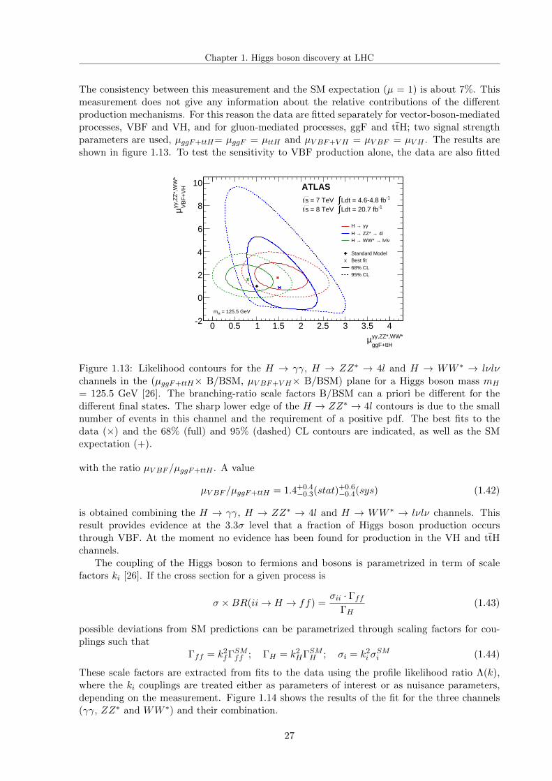
The consistency between this measurement and the SM expectation (µ = 1) is about 7%. Thismeasurement does not give any information about the relative contributions of the differentproduction mechanisms. For this reason the data are fitted separately for vector-boson-mediatedprocesses, VBF and VH, and for gluon-mediated processes, ggF and ttH; two signal strengthparameters are used, µggF+ttH= µggF = µttH and µV BF+V H = µV BF = µV H . The results areshown in figure 1.13. To test the sensitivity to VBF production alone, the data are also fitted
ggF+ttH
,ZZ*,WW*γγµ0 0.5 1 1.5 2 2.5 3 3.5 4
VB
F+
VH
,ZZ
*,W
W*
γγµ
-2
0
2
4
6
8
10
Standard ModelBest fit68% CL95% CL
γγ →H
4l→ ZZ* →H νlν l→ WW* →H
ATLAS -1Ldt = 4.6-4.8 fb∫ = 7 TeV s
-1Ldt = 20.7 fb∫ = 8 TeV s
= 125.5 GeVHm
Figure 1.13: Likelihood contours for the H → γγ, H → ZZ∗ → 4l and H → WW ∗ → lνlνchannels in the (µggF+ttH× B/BSM, µV BF+V H× B/BSM) plane for a Higgs boson mass mH
= 125.5 GeV [26]. The branching-ratio scale factors B/BSM can a priori be different for thedifferent final states. The sharp lower edge of the H → ZZ∗ → 4l contours is due to the smallnumber of events in this channel and the requirement of a positive pdf. The best fits to thedata (×) and the 68% (full) and 95% (dashed) CL contours are indicated, as well as the SMexpectation (+).
with the ratio µV BF /µggF+ttH . A value
µV BF /µggF+ttH = 1.4+0.4−0.3(stat)+0.6
−0.4(sys) (1.42)
is obtained combining the H → γγ, H → ZZ∗ → 4l and H → WW ∗ → lνlν channels. Thisresult provides evidence at the 3.3σ level that a fraction of Higgs boson production occursthrough VBF. At the moment no evidence has been found for production in the VH and ttHchannels.
The coupling of the Higgs boson to fermions and bosons is parametrized in term of scalefactors ki [26]. If the cross section for a given process is
σ ×BR(ii→ H → ff) =σii · Γff
ΓH(1.43)
possible deviations from SM predictions can be parametrized through scaling factors for cou-plings such that
Γff = k2fΓSMff ; ΓH = k2
HΓSMH ; σi = k2i σ
SMi (1.44)
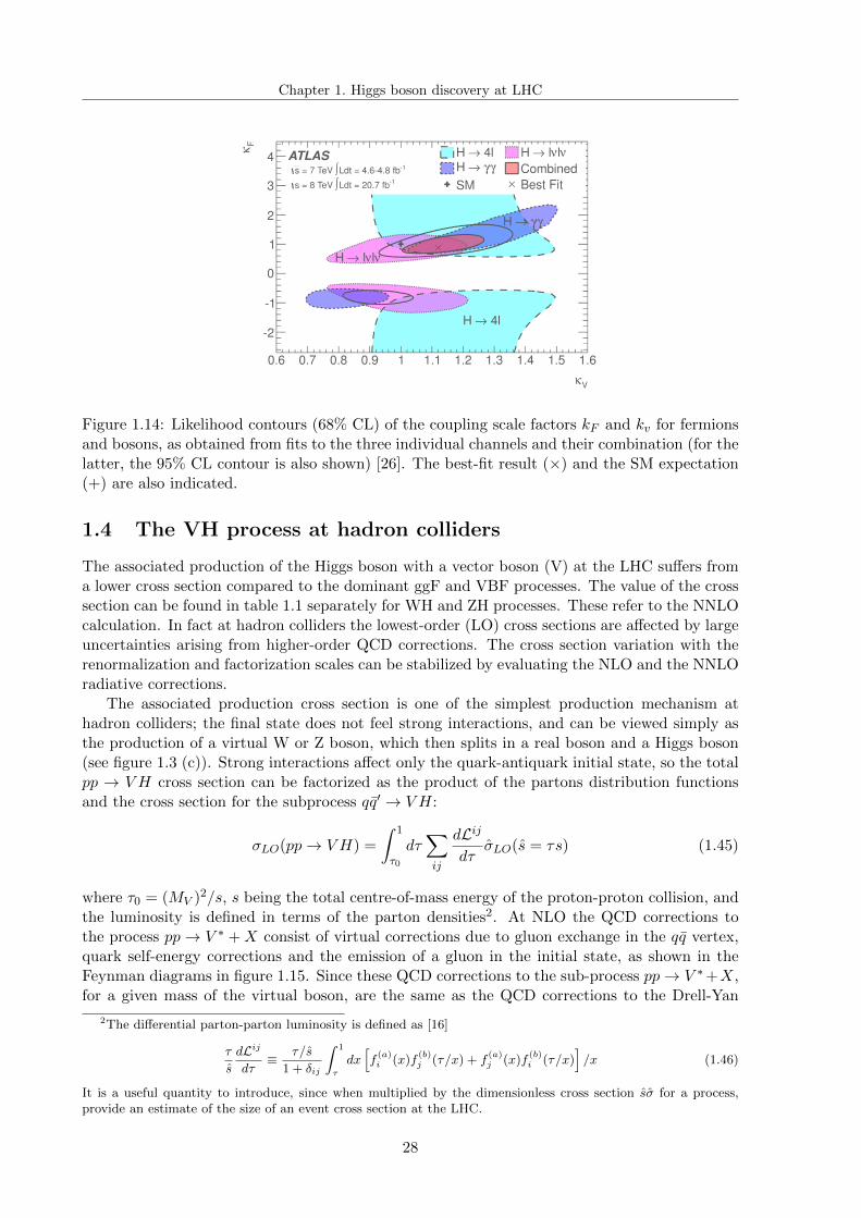
These scale factors are extracted from fits to the data using the profile likelihood ratio Λ(k),where the ki couplings are treated either as parameters of interest or as nuisance parameters,depending on the measurement. Figure 1.14 shows the results of the fit for the three channels(γγ, ZZ∗ and WW ∗) and their combination.
27
Chapter 1. Higgs boson discovery at LHC
Figure 1.14: Likelihood contours (68% CL) of the coupling scale factors kF and kv for fermionsand bosons, as obtained from fits to the three individual channels and their combination (for thelatter, the 95% CL contour is also shown) [26]. The best-fit result (×) and the SM expectation(+) are also indicated.
1.4 The VH process at hadron colliders
The associated production of the Higgs boson with a vector boson (V) at the LHC suffers froma lower cross section compared to the dominant ggF and VBF processes. The value of the crosssection can be found in table 1.1 separately for WH and ZH processes. These refer to the NNLOcalculation. In fact at hadron colliders the lowest-order (LO) cross sections are affected by largeuncertainties arising from higher-order QCD corrections. The cross section variation with therenormalization and factorization scales can be stabilized by evaluating the NLO and the NNLOradiative corrections.
The associated production cross section is one of the simplest production mechanism athadron colliders; the final state does not feel strong interactions, and can be viewed simply asthe production of a virtual W or Z boson, which then splits in a real boson and a Higgs boson(see figure 1.3 (c)). Strong interactions affect only the quark-antiquark initial state, so the totalpp → V H cross section can be factorized as the product of the partons distribution functionsand the cross section for the subprocess qq′ → V H:
σLO(pp→ V H) =
∫ 1
τ0
dτ∑ij
dLij
dτσLO(s = τs) (1.45)
where τ0 = (MV )2/s, s being the total centre-of-mass energy of the proton-proton collision, andthe luminosity is defined in terms of the parton densities2. At NLO the QCD corrections tothe process pp→ V ∗ +X consist of virtual corrections due to gluon exchange in the qq vertex,quark self-energy corrections and the emission of a gluon in the initial state, as shown in theFeynman diagrams in figure 1.15. Since these QCD corrections to the sub-process pp→ V ∗+X,for a given mass of the virtual boson, are the same as the QCD corrections to the Drell-Yan
2The differential parton-parton luminosity is defined as [16]
τ
s
dLij
dτ≡ τ/s
1 + δij
∫ 1
τ
dx[f(a)i (x)f
(b)j (τ/x) + f
(a)j (x)f
(b)i (τ/x)
]/x (1.46)
It is a useful quantity to introduce, since when multiplied by the dimensionless cross section sσ for a process,provide an estimate of the size of an event cross section at the LHC.
28
Chapter 1. Higgs boson discovery at LHC
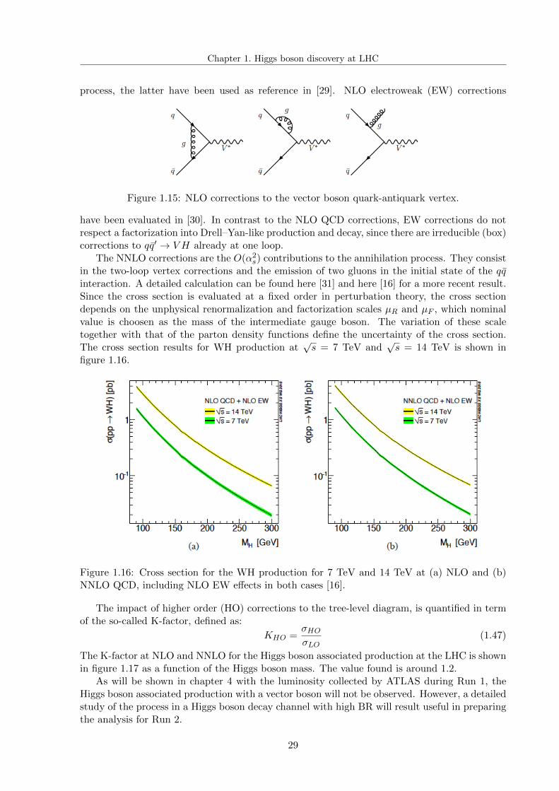
process, the latter have been used as reference in [29]. NLO electroweak (EW) corrections
Figure 1.15: NLO corrections to the vector boson quark-antiquark vertex.
have been evaluated in [30]. In contrast to the NLO QCD corrections, EW corrections do notrespect a factorization into Drell–Yan-like production and decay, since there are irreducible (box)corrections to qq′ → V H already at one loop.
The NNLO corrections are the O(α2s) contributions to the annihilation process. They consist
in the two-loop vertex corrections and the emission of two gluons in the initial state of the qqinteraction. A detailed calculation can be found here [31] and here [16] for a more recent result.Since the cross section is evaluated at a fixed order in perturbation theory, the cross sectiondepends on the unphysical renormalization and factorization scales µR and µF , which nominalvalue is choosen as the mass of the intermediate gauge boson. The variation of these scaletogether with that of the parton density functions define the uncertainty of the cross section.The cross section results for WH production at
√s = 7 TeV and
√s = 14 TeV is shown in
figure 1.16.
Figure 1.16: Cross section for the WH production for 7 TeV and 14 TeV at (a) NLO and (b)NNLO QCD, including NLO EW effects in both cases [16].
The impact of higher order (HO) corrections to the tree-level diagram, is quantified in termof the so-called K-factor, defined as:
KHO =σHOσLO
(1.47)
The K-factor at NLO and NNLO for the Higgs boson associated production at the LHC is shownin figure 1.17 as a function of the Higgs boson mass. The value found is around 1.2.
As will be shown in chapter 4 with the luminosity collected by ATLAS during Run 1, theHiggs boson associated production with a vector boson will not be observed. However, a detailedstudy of the process in a Higgs boson decay channel with high BR will result useful in preparingthe analysis for Run 2.
29
Chapter 1. Higgs boson discovery at LHC
Figure 1.17: The K-factors (ratio to LO prediction) for pp → WH at the LHC 7 TeV as afunction of mH for the NLO and NNLO cross sections [16]. The little kinks at around 160 GeVand, somewhat smaller, 180 GeV, are due to the WW and ZZ thresholds that occur in the EWradiative corrections.
30
Chapter 2
The ATLAS detector
In this chapter the experimental apparatus used to measure the VH process explained in theprevious chapter is described. ATLAS is a general-purpose experiment recording the collisionsprovided by the Large Hadron Collider (LHC), the proton-proton collider which is operationalat CERN since 2009. The ATLAS detector is going to be explained in all its sub-componentsin the next sections.
2.1 The Large Hadron Collider
The Large Hadron Collider [28] is the 27 km long particle collider hosted in the same tunnelwhere the LEP collider was, about 100 meters underneath the Swiss-French national bordernear Geneva. It is the most energetic particle collider ever built. In the LHC ring two protonbunches at a time collide, each bunch having approximately 1011 protons, with a centre-of-massenergy equals to
√s= 8 TeV during 2012 data taking period (2012 was part of the so-called
Run 1 ). The proton-proton (pp) collider is currently in a shutdown phase, to allow for thereplacement and upgrade of some machine and detectors components; it will start again withprotons collisions in spring 2015, with a centre-of-mass energy of 13 TeV.
Before particles are injected into the LHC they go through several acceleration stages, shownin figure 2.1. After their production, the proton beams are accelerated up to 50 MeV by theLINAC2 machine. The protons are then injected into the Proton Synchrotron Booster (PSB)which accelerate the particles to 1.4 GeV. After that, the particles are injected first into theProton Synchrotron (PS) where they are accelerated to 26 GeV, and then into the Super ProtonSynchrotron (SPS) which increases their energy to 450 GeV. The particles enter the LHC intotwo parallel rings and after ramping up to the desired energy the beams are squeezed and directedto collisions in the dedicated LHC experiments. Beams focusing and acceleration is obtainedwith magnets and radiofrequency (RF) cavities: LHC is equipped with 1232 superconductingmagnets and 6 RF cavities which bend and accelerate the proton beams in the two parallelbeam lines in the machine. The magnetic field used to bend such energetic protons is of 8.3 T.For reaching and keeping the superconductivity range of the cold masses, the cooling systemprovides the magnets with fluid helium at a temperature of 1.9 K.
In studying high energy particle collisions one of the crucial parameter of the collider is theinstantaneous luminosity, since it is proportional to the production rate:
dN
dt= L × σ (2.1)
where σ is the cross section of the considered process. The instantaneous luminosity depends
31
Chapter 2. The ATLAS detector
Figure 2.1: The CERN particles accelerator complex. The injection chain together with the fourinteraction points are visible.
on the intrinsic properties of the machine:
L =fNp
2k
4πσxσy(2.2)
where Np is the number of particles in a bunch, f is the revolution frequency of the protonin the accelerating ring, k is the number of bunches circulating in the beam, σx and σy arethe gaussian beam profiles in the transverse plane with respect to the beam direction. A goodknowledge of the expected beam properties give access to a good expectation value for theluminosity. The luminosity can then be used in two ways from equation (2.1): either predictthe number of expected background or signal events from a prior cross section value, or measurea cross section from a number of observed events in data. To reduce the uncertainty on theluminosity and hence on the measured cross sections, its value is monitored regularly duringthe data-taking period, for example with the Van Der Meer scans method [32]. Figure 2.2shows the peak luminosity delivered to ATLAS in the various data-taking period of Run1, whilethe 2012 integrated luminosity used for the scope of this thesis, corresponds to 20.3 fb−1 (seepicture 4.4). Although the high intensity of the beams allows to probe for rare process, it alsogives rise to some disadvantages, as the possibility to have more than one interaction per bunchcrossing. This penomenon is called pile-up. We distinguish between in time pile-up, when manyinteractions arise from the same bunches collision, and out-of-time pile-up, when detector signalsoccured in a bunch crossing before the event of interest but are recorded later because of thelatency time of some detectors. In both cases the pile-up produces a high particle multiplicityin the detector which makes harder the reconstruction of the event of interest. The averagenumber of pile-up interactions in 2012 collisions was < µ > = 20.7.
Table 2.1 shows the LHC parameters in 2012. The LHC provides collisions in four collisionpoints along its circumference where detector experiments are hosted: ALICE (A Large IonCollider Experiment) [33], ATLAS (A Toroidal Lhc ApparatuS ) [34], CMS (Compact MuonSolenoid) [35][36] and LHCb (Large Hadron Collider beauty) [37]. ATLAS and CMS are multi-
32
Chapter 2. The ATLAS detector
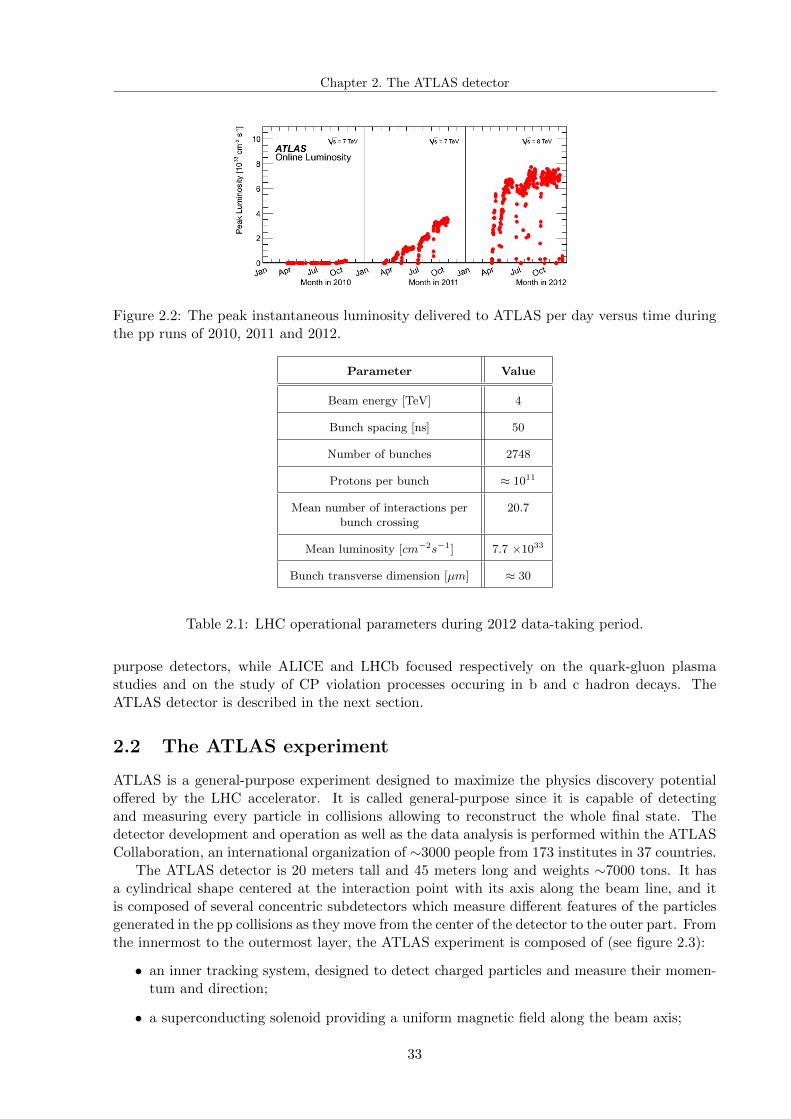
Figure 2.2: The peak instantaneous luminosity delivered to ATLAS per day versus time duringthe pp runs of 2010, 2011 and 2012.
Parameter Value
Beam energy [TeV] 4
Bunch spacing [ns] 50
Number of bunches 2748
Protons per bunch ≈ 1011
Mean number of interactions perbunch crossing
20.7
Mean luminosity [cm−2s−1] 7.7 ×1033
Bunch transverse dimension [µm] ≈ 30
Table 2.1: LHC operational parameters during 2012 data-taking period.
purpose detectors, while ALICE and LHCb focused respectively on the quark-gluon plasmastudies and on the study of CP violation processes occuring in b and c hadron decays. TheATLAS detector is described in the next section.
2.2 The ATLAS experiment
ATLAS is a general-purpose experiment designed to maximize the physics discovery potentialoffered by the LHC accelerator. It is called general-purpose since it is capable of detectingand measuring every particle in collisions allowing to reconstruct the whole final state. Thedetector development and operation as well as the data analysis is performed within the ATLASCollaboration, an international organization of ∼3000 people from 173 institutes in 37 countries.
The ATLAS detector is 20 meters tall and 45 meters long and weights ∼7000 tons. It hasa cylindrical shape centered at the interaction point with its axis along the beam line, and itis composed of several concentric subdetectors which measure different features of the particlesgenerated in the pp collisions as they move from the center of the detector to the outer part. Fromthe innermost to the outermost layer, the ATLAS experiment is composed of (see figure 2.3):
• an inner tracking system, designed to detect charged particles and measure their momen-tum and direction;
• a superconducting solenoid providing a uniform magnetic field along the beam axis;
33
Chapter 2. The ATLAS detector
• a calorimeter system, with an electromagnetic calorimeter to measure the energy depositedby electrons and photons, followed by hadronic calorimeter;
• a muon spectrometer, to reconstruct the muon tracks and to measure their momentum, ina system of an air-cored toroidal magnets.
Figure 2.3: Schematic design of the ATLAS detector.
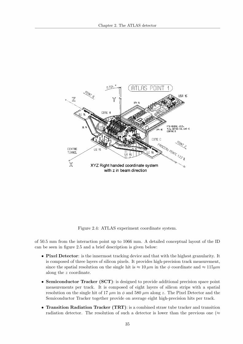
2.2.1 ATLAS coordinate system
The ATLAS reference system is shown in figure 2.4: the origin of the system is in the nominalinteraction point, the z axis is along the beam line, while the x−y plane is the plane perpendicularwith respect to beam line. The positive x-axis is defined as pointing from the interaction pointto the centre of the LHC ring and the positive y-axis is defined as pointing upwards. Theazimuthal angle φ is defined around the beam axis, while the polar angle θ is the angle from thez axis in the y − z plane. The θ variable is not invariant under boosts along the z axis, and sothe rapidity y is used:
y =1
2lnE + p cosθ
E − p cosθ(2.3)
where E and p are respectively the energy and the momentum of the particle. In the ultra-relativistic limit the pseudorapidity η is a very good approximation of y:
η = −ln[tan
(θ
2
)](2.4)
With the relation in equation (2.4) to smaller values of η correspond higher θ angles and viceversa.
2.2.2 The Inner detector
The ATLAS Inner detector (ID) has a fully coverage in φ and covers the pseudorapidity range|η| < 2.5. It consists of a silicon Pixel detector (Pixel), silicon strip detector (SCT) and for|η| < 2 a Transition Radiation Tracker (TRT). This set of detectors covers the radial distance
34
Chapter 2. The ATLAS detector
Figure 2.4: ATLAS experiment coordinate system.
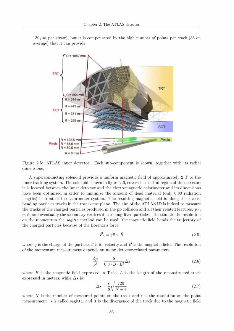
of 50.5 mm from the interaction point up to 1066 mm. A detailed conceptual layout of the IDcan be seen in figure 2.5 and a brief description is given below:
• Pixel Detector: is the innermost tracking device and that with the highest granularity. Itis composed of three layers of silicon pixels. It provides high-precision track measurement,since the spatial resolution on the single hit is ≈ 10µm in the φ coordinate and ≈ 115µmalong the z coordinate.
• Semiconductor Tracker (SCT): is designed to provide additional precision space pointmeasurements per track. It is composed of eight layers of silicon strips with a spatialresolution on the single hit of 17 µm in φ and 580 µm along z. The Pixel Detector and theSemiconductor Tracker together provide on average eight high-precision hits per track.
• Transition Radiation Tracker (TRT): is a combined straw tube tracker and transitionradiation detector. The resolution of such a detector is lower than the previous one (≈
35
Chapter 2. The ATLAS detector
130µm per straw), but it is compensated by the high number of points per track (36 onaverage) that it can provide.
Figure 2.5: ATLAS inner detector. Each sub-component is shown, together with its radialdimensions.
A superconducting solenoid provides a uniform magnetic field of approximately 2 T to theinner tracking system. The solenoid, shown in figure 2.6, covers the central region of the detector;it is located between the inner detector and the electromagnetic calorimeter and its dimensionshave been optimized in order to minimize the amount of dead material (only 0.83 radiationlengths) in front of the calorimeter system. The resulting magnetic field is along the z axis,bending particles tracks in the transverse plane. The aim of the ATLAS ID is indeed to measurethe tracks of the charged particles produced in the pp collision and all their related features: pT ,η, φ, and eventually the secondary vertices due to long-lived particles. To estimate the resolutionon the momentum the sagitta method can be used: the magnetic field bends the trajectory ofthe charged particles because of the Lorentz’s force:
~FL = q~v × ~B (2.5)
where q is the charge of the particle, ~v is its velocity and ~B is the magnetic field. The resolutionof the momentum measurement depends on many detector-related parameters:
δp
p2=
8
0.3 ·B · L2∆s (2.6)
where B is the magnetic field expressed in Tesla, L is the length of the reconstructed trackexpressed in meters, while ∆s is:
∆s =ε
8
√720
N + 4(2.7)
where N is the number of measured points on the track and ε is the resolution on the pointmeasurement. s is called sagitta, and it is the divergence of the track due to the magnetic field
36
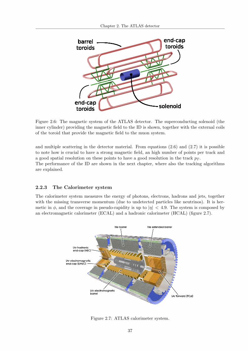
Chapter 2. The ATLAS detector
Figure 2.6: The magnetic system of the ATLAS detector. The superconducting solenoid (theinner cylinder) providing the magnetic field to the ID is shown, together with the external coilsof the toroid that provide the magnetic field to the muon system.
and multiple scattering in the detector material. From equations (2.6) and (2.7) it is possibleto note how is crucial to have a strong magnetic field, an high number of points per track anda good spatial resolution on these points to have a good resolution in the track pT .The performance of the ID are shown in the next chapter, where also the tracking algorithmsare explained.
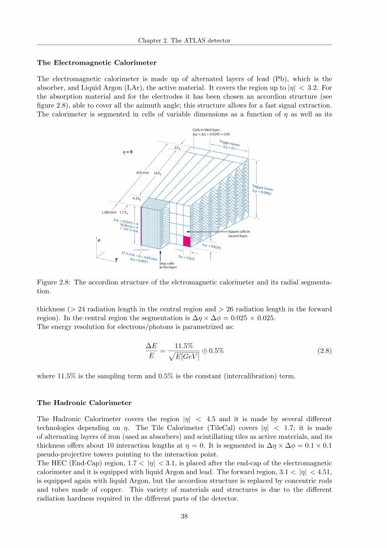
2.2.3 The Calorimeter system
The calorimeter system measures the energy of photons, electrons, hadrons and jets, togetherwith the missing transverse momentum (due to undetected particles like neutrinos). It is her-metic in φ, and the coverage in pseudo-rapidity is up to |η| < 4.9. The system is composed byan electromagnetic calorimeter (ECAL) and a hadronic calorimeter (HCAL) (figure 2.7).
Figure 2.7: ATLAS calorimeter system.
37
Chapter 2. The ATLAS detector
The Electromagnetic Calorimeter
The electromagnetic calorimeter is made up of alternated layers of lead (Pb), which is theabsorber, and Liquid Argon (LAr), the active material. It covers the region up to |η| < 3.2. Forthe absorption material and for the electrodes it has been chosen an accordion structure (seefigure 2.8), able to cover all the azimuth angle; this structure allows for a fast signal extraction.The calorimeter is segmented in cells of variable dimensions as a function of η as well as its
Figure 2.8: The accordion structure of the elctromagnetic calorimeter and its radial segmenta-tion.
thickness (> 24 radiation length in the central region and > 26 radiation length in the forwardregion). In the central region the segmentation is ∆η ×∆φ = 0.025 × 0.025.The energy resolution for electrons/photons is parametrized as:
∆E
E=
11.5%√E[GeV ]
⊕ 0.5% (2.8)
where 11.5% is the sampling term and 0.5% is the constant (intercalibration) term.
The Hadronic Calorimeter
The Hadronic Calorimeter covers the region |η| < 4.5 and it is made by several differenttechnologies depending on η. The Tile Calorimeter (TileCal) covers |η| < 1.7; it is madeof alternating layers of iron (used as absorbers) and scintillating tiles as active materials, and itsthickness offers about 10 interaction lengths at η = 0. It is segmented in ∆η ×∆φ = 0.1× 0.1pseudo-projective towers pointing to the interaction point.The HEC (End-Cap) region, 1.7 < |η| < 3.1, is placed after the end-cap of the electromagneticcalorimeter and it is equipped with liquid Argon and lead. The forward region, 3.1 < |η| < 4.51,is equipped again with liquid Argon, but the accordion structure is replaced by concentric rodsand tubes made of copper. This variety of materials and structures is due to the differentradiation hardness required in the different parts of the detector.
38
Chapter 2. The ATLAS detector
2.2.4 The Muon Spectrometer
The Muon Spectrometer (MS) is the outermost component of the ATLAS detector. It is designedto detect minimum ionizing particles (muons) exiting the calorimeter system and to measuretheir momenta in the pseudorapidity range |η| < 2.7. The MS is instrumented with bothtrigger and high-precision chambers immersed in the magnetic field provided by air-core toroidalmagnets (figure 2.6) which bends the particles along the η coordinate (being
∫B · dl between
2 and 6 T · m). A sketch of the MS is displayed in figure 2.9. The MS chambers devoted to
Figure 2.9: The ATLAS muon spectrometer.
the precision tracking are the Monitored Drift Tubes (MDT) and the Cathode Strip Chambers(CSC), while for the trigger measurement the Resistive Plate Chambers (RPC) and the ThinGap Chambers (TGC) are respectively in the barrel and in the endcap:
• Monitored Drift Tubes: they are used in the central region (|η| < 2) of the detector.The MDT chambers are composed of aluminium tubes of 30 mm diameter and 400 µmthickness, with a 50 µm diameter central wire. The tubes are filled with a mixture ofArgon and CO2 at high pressure (3 bars), and each tube has a spatial resolution of 80 µm.
• Cathode Strip Chambers: they are used at higher pseudo-rapidity (2 < |η| < 2.7)with respect to the MDT. CSC chambers are multiwire proportional chambers in which thereadout is performed using strips forming a grid on the cathode plane in both orthogonaland parallel direction with respect to the wire. The spatial resolution of the CSC is about60 µm.
• Resistive Plate Chambers: the RPC produce the trigger signal in the barrel. They arealso capable to measure the transverse coordinate and are therefore complementary withthe MDT. 544 chambers are located in three concentric layers connected to the MDT.Every chamber has 2-layers of gas gap filled with a gas mixture of 94.74% C2H2F4 + 5%isoC4H10 + 0.3% SF6, where the last one is added to limit the charge avalanches in thechamber. The chambers are made with bakelite plates of 2 mm and readout strips withpitches of about 3 cm. The RPC work at 9.8 kV and have a time resolution of 1.5 ns.
• Thin Gap Chambers: the TGC are multiwire proportional chambers dedicated to thetrigger system on the endcap part of the ATLAS detector. The TGC, like the RPC,
39
Chapter 2. The ATLAS detector
provide also a measurement of the muon track coordinate orthogonal to the one providedby the precision tracking chambers. The nominal spatial resolution for the TGC its 3.7mm in the R − φ plane. The gas mixture used for these chambers is 55% CO2 + 45%nC5H12 and they work at 2.9 kV. The time resolution is about 4 ns.
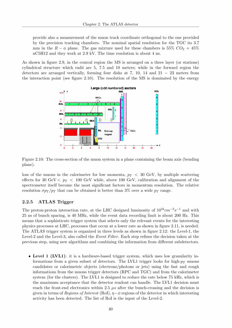
As shown in figure 2.9, in the central region the MS is arranged on a three layer (or stations)cylindrical structure which radii are 5, 7.5 and 10 meters; while in the forward region thedetectors are arranged vertically, forming four disks at 7, 10, 14 and 21 − 23 meters fromthe interaction point (see figure 2.10). The resolution of the MS is dominated by the energy
Figure 2.10: The cross-section of the muon system in a plane containing the beam axis (bendingplane).
loss of the muons in the calorimeter for low momenta, pT < 30 GeV, by multiple scatteringeffects for 30 GeV< pT < 100 GeV while, above 100 GeV, calibration and alignment of thespectrometer itself become the most significant factors in momentum resolution. The relativeresolution σpT /pT that can be obtained is better than 3% over a wide pT range.
2.2.5 ATLAS Trigger
The proton-proton interaction rate, at the LHC designed luminosity of 1034cm−2s−1 and with25 ns of bunch spacing, is 40 MHz, while the event data recording limit is about 200 Hz. Thismeans that a sophisticate trigger system that selects only the relevant events for the interestingphysics processes at LHC, processes that occur at a lower rate as shown in figure 2.11, is needed.The ATLAS trigger system is organized in three levels as shown in figure 2.12: the Level-1, theLevel-2 and the Level-3, also called the Event Filter. Each step refines the decision taken at theprevious step, using new algorithms and combining the information from different subdetectors.
• Level 1 (LVL1): it is a hardware-based trigger system, which uses low granularity in-formations from a given subset of detectors. The LVL1 trigger looks for high-pT muonscandidates or calorimetric objects (electrons/photons or jets) using the fast and roughinformations from the muons trigger detectors (RPC and TGC) and from the calorimetersystem (for the clusters). The LVL1 is designed to reduce the rate below 75 kHz, which isthe maximum acceptance that the detector readout can handle. The LVL1 decision mustreach the front-end electronics within 2.5 µs after the bunch-crossing and the decision isgiven in terms of Regions of Interest (RoI), η−φ regions of the detector in which interestingactivity has been detected. The list of RoI is the input of the Level-2.
40
Chapter 2. The ATLAS detector
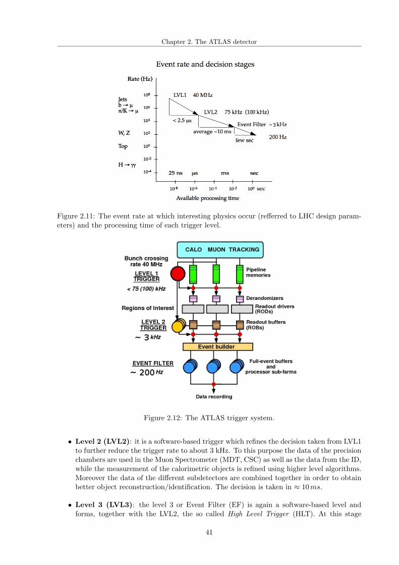
Figure 2.11: The event rate at which interesting physics occur (refferred to LHC design param-eters) and the processing time of each trigger level.
Figure 2.12: The ATLAS trigger system.
• Level 2 (LVL2): it is a software-based trigger which refines the decision taken from LVL1to further reduce the trigger rate to about 3 kHz. To this purpose the data of the precisionchambers are used in the Muon Spectrometer (MDT, CSC) as well as the data from the ID,while the measurement of the calorimetric objects is refined using higher level algorithms.Moreover the data of the different subdetectors are combined together in order to obtainbetter object reconstruction/identification. The decision is taken in ≈ 10ms.
• Level 3 (LVL3): the level 3 or Event Filter (EF) is again a software-based level andforms, together with the LVL2, the so called High Level Trigger (HLT). At this stage
41
Chapter 2. The ATLAS detector
the reconstruction algorithms, also used during the offline event reconstruction, are used,and a full reconstruction is performed. The output rate of the LVL3 is of the order of≈ 100 Hz. All the events that have been selected by the LVL3 trigger are then written tomass storage (disks or tapes), and are then used in the analysis.
42
Chapter 3
Physics objects definition andreconstruction
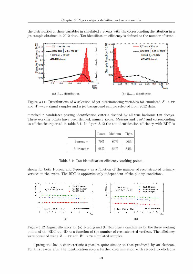
The analysis described in this thesis relies on the off-line reconstruction of electrons, muons,taus and jets, together with the determination of the missing transverse momentum. Thischapter describes the main algorithms used for objects reconstruction in ATLAS during Run1data taking period, while analysis specific object selection criteria are described in detail inchapter 4.
3.1 Track reconstruction
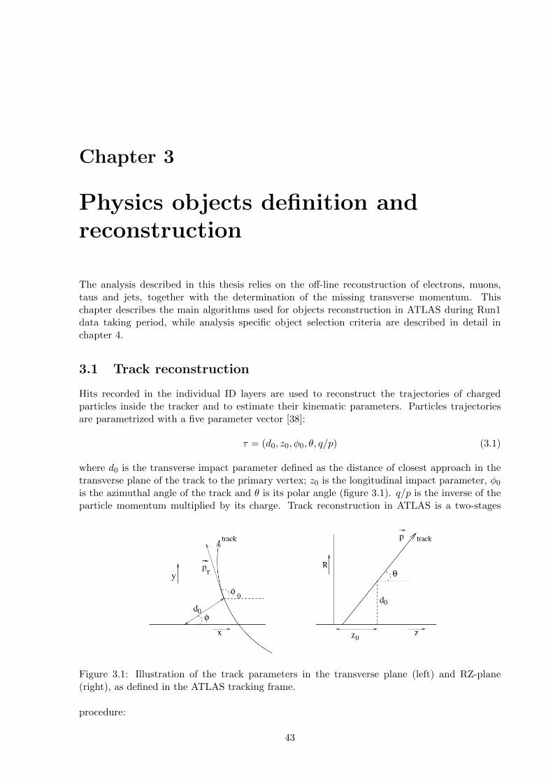
Hits recorded in the individual ID layers are used to reconstruct the trajectories of chargedparticles inside the tracker and to estimate their kinematic parameters. Particles trajectoriesare parametrized with a five parameter vector [38]:
τ = (d0, z0, φ0, θ, q/p) (3.1)
where d0 is the transverse impact parameter defined as the distance of closest approach in thetransverse plane of the track to the primary vertex; z0 is the longitudinal impact parameter, φ0
is the azimuthal angle of the track and θ is its polar angle (figure 3.1). q/p is the inverse of theparticle momentum multiplied by its charge. Track reconstruction in ATLAS is a two-stages
Figure 3.1: Illustration of the track parameters in the transverse plane (left) and RZ-plane(right), as defined in the ATLAS tracking frame.
procedure:
43
Chapter 3. Physics objects definition and reconstruction
Track finder: Assignment of the hits left in the detector by charged particles traversing activedetector elements to the track candidate.
Track fitter: The hits are used to reconstruct the trajectories by performing a fit to the trackkinematic parameters. The track fitting is based on the minimization of the track-hitresiduals.
In the above procedure a sequence of algorithms is used [39]. The default, named inside-outalgorithm, starts with combining hits from the three pixel detector layers and the first SCTlayer, in the so-called track seed. This seed is then extended to all the SCT candidates to form atrack candidate that is then extended into the TRT and refitted using the full ID information. Ifsome TRT hit worsening the fit quality is found, this is not included in the final fit and is labelledas outlier and kept for off-line studies. A track in the barrel region of the ID has typically 3Pixel hits, 8 SCT hits and approximately 30 TRT hits.
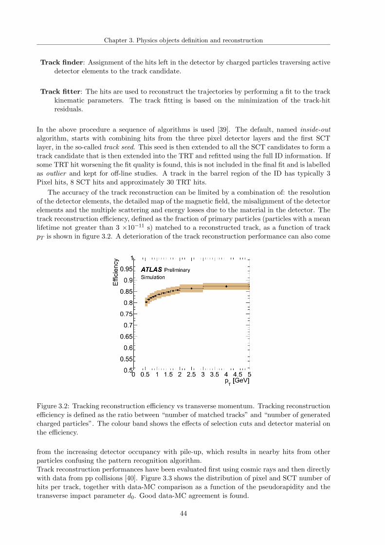
The accuracy of the track reconstruction can be limited by a combination of: the resolutionof the detector elements, the detailed map of the magnetic field, the misalignment of the detectorelements and the multiple scattering and energy losses due to the material in the detector. Thetrack reconstruction efficiency, defined as the fraction of primary particles (particles with a meanlifetime not greater than 3 ×10⁻¹¹ s) matched to a reconstructed track, as a function of trackpT is shown in figure 3.2. A deterioration of the track reconstruction performance can also come
Figure 3.2: Tracking reconstruction efficiency vs transverse momentum. Tracking reconstructionefficiency is defined as the ratio between “number of matched tracks” and “number of generatedcharged particles”. The colour band shows the effects of selection cuts and detector material onthe efficiency.
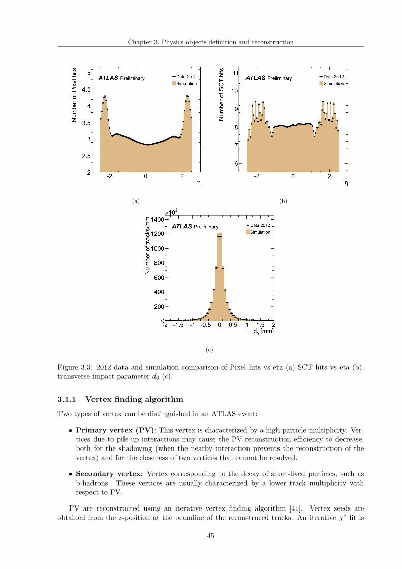
from the increasing detector occupancy with pile-up, which results in nearby hits from otherparticles confusing the pattern recognition algorithm.Track reconstruction performances have been evaluated first using cosmic rays and then directlywith data from pp collisions [40]. Figure 3.3 shows the distribution of pixel and SCT number ofhits per track, together with data-MC comparison as a function of the pseudorapidity and thetransverse impact parameter d0. Good data-MC agreement is found.
44
Chapter 3. Physics objects definition and reconstruction
(a) (b)
(c)
Figure 3.3: 2012 data and simulation comparison of Pixel hits vs eta (a) SCT hits vs eta (b),transverse impact parameter d0 (c).
3.1.1 Vertex finding algorithm
Two types of vertex can be distinguished in an ATLAS event:
• Primary vertex (PV): This vertex is characterized by a high particle multiplicity. Ver-tices due to pile-up interactions may cause the PV reconstruction efficiency to decrease,both for the shadowing (when the nearby interaction prevents the reconstruction of thevertex) and for the closeness of two vertices that cannot be resolved.
• Secondary vertex: Vertex corresponding to the decay of short-lived particles, such asb-hadrons. These vertices are usually characterized by a lower track multiplicity withrespect to PV.
PV are reconstructed using an iterative vertex finding algorithm [41]. Vertex seeds areobtained from the z-position at the beamline of the reconstruced tracks. An iterative χ2 fit is
45
Chapter 3. Physics objects definition and reconstruction
made by using seed and nearby tracks. Each track carries a weight that is a measure of itscompatibility with the fitted vertex. Tracks displaced by more than 7σ from the vertex are usedto seed a new vertex. The procedure goes on until no additional vertices are found. At leasttwo charged particles with |η| < 2.5 and pT > 400 MeV are required to define the interaction.
Figure 3.4 shows the number of reconstructed vertices per event in 2012 data, as a functionof the number of pile-up interactions. Data are compared with MC expectations.
Figure 3.4: Average number of reconstructed primary vertices per event as a function of averagenumber of pp interactions per bunch crossing measured for the data of 2012. Data are collectedusing a minimum bias trigger. A second order polynomial fit is performed in the upper rangeof µ. For the lower values of µ the result of extrapolation is shown.
3.2 Leptons
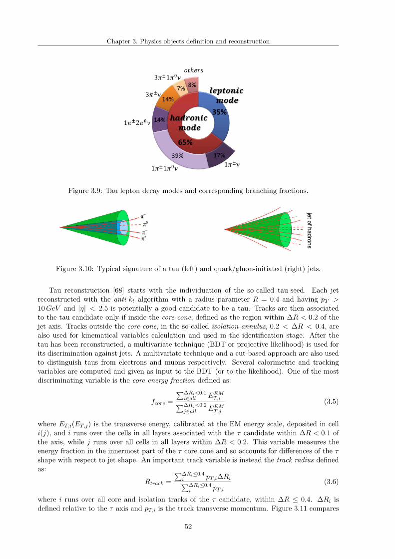
Leptons represent the final state of the process studied in this thesis. Their signature and theprocedure adopted in ATLAS for their reconstruction and identification is the subject of thissection. Tau lepton reconstruction is postponed after the jet reconstruction; the reason for thiswill become clear in going further with the chapter.
3.2.1 Electron reconstruction
The characteristic signature of electrons consists in a track in the ID together with a narrowshower in the EM calorimeter. Electrons reconstruction uses different algorithms depending onwhere the electron is found: we refer to central electron, if the electron is in |η| < 2.5, and toforward electron, if it is in 2.5 < |η| < 4.9 [42]. An electron in the central region is reconstructedwith an algorithm that combines the energy deposit in the EM with the track in the ID. Firstthe EM cluster is built using the so-called sliding window algorithm, which adds together energydeposits with window size 3 × 5 in units of 0.025×0.05 in (η,φ) space. Then the reconstructedtrack is extrapolated from the ID to the EM calorimeter to look for a matching with the cluster.A track and a cluster are considered to be succesfully matched if the distance between the trackimpact point and the EM cluster barycentre is |∆η| < 0.05. An electron candidate is consideredto be reconstructed if at least one track is matched to the seed cluster. The four-momentum ofcentral electrons is computed using information from both the final cluster and the best trackmatched to the seed cluster.
Forward electrons are instead reconstructed using only the information from the EMEC andthe forward calorimeter. No distinction is then possible between electrons and photons. Atopological cluster algorithm is used: cells with deposited energy significantly above the noise
46
Chapter 3. Physics objects definition and reconstruction
level are grouped in three dimensions in an iterative procedure, starting from seed cells. Dueto the reduced detector information forward electrons are used in physics analysis only forET > 20GeV .
Once the reconstructed candidate electron is found an identification criterion is applied,which relies on the shape of electromagnetic shower in the calorimeter as well as on tracking andtrack-to-cluster matching quantities. The identification can be based either on independent cutson these quantities or on a single cut on the output of a likelihood function taking as input thesequantities. Three reference sets of cuts have been defined with increasing background rejectionpower: loose, medium and tight. In general, each cut adds to the previous some additionalrequirements. From these categories, three more categories are derived, named ”++” . Theywere added in order to accomplish the trigger bandwidth restrictions for high luminosity, andhave been used in most of 2012 ATLAS data analysis:
• Loose++: Is based on calorimeter informations only. Shower shape variables of the EMcalorimeter middle layer and hadronic leakage variables are used. The hadronic leakage(Rhad) allows to distinguish electron shower from hadrons shower, thanks to the differentwidth of the two (usually electron showers have narrower width in η than those createdby jets). It is defined as the ratio of the transverse energy reconstructed in the first layerof the hadronic calorimeter to the transverse energy reconstructed in the EM calorimeter.This category has a high identification efficiency (≈ 97%) but poor background rejection.
• Medium++: With respect to the previous category this adds information from the firstlayer of the EM calorimeter, aimed to improve the e − π separation. In addition furtherqualities on the ID tracks are requested. A background rejection of a factor 3-4 higherthan the loose++ category is achieved, while the identification efficiency is reduced byabout 10%.
• Tight++: This category adds many additional selections, as the particle identificationusing the TRT, the discrimination against photon conversions via a b-layer hit requirementand information about reconstructed conversion vertices. Background rejection is ≈ 105
while the identification efficiency is ≈ 80%.
For the scope of this thesis the identification based on a likelihood output has been used. Theelectron likelihood makes use of signal and background probability density functions (PDF) ofthe discriminating variables. Based on these PDF, an overall probability is calculated for theobject to be signal or background. The signal and background probabilities are combined into adiscriminant on which a cut is applied. The electron reconstruction efficiency measured in 2011and 2012 data is shown in figure 3.5, while figure 3.6 shows the electron identification efficiencyfor the Loose likelihood selection (LooseLLH) and the Tight++ selection (VeryTightLLH) in2012 data [43].
3.2.2 Muon reconstruction
Muon reconstruction uses the available information of MS and ID systems, and partially theinformation of the calorimeter. Several reconstruction criteria are used, leading to different typesof muons [44]:
• Stand-alone (SA) muon: only the hits in the MS stations are used to reconstruct the muontrack. The hits are combined to form segments that are then used in a fit for the trackreconstruction. The track is then extrapolated back to the point of closest approach tothe beam line, taking into account the energy loss in the calorimeter. SA muons are usedto extend the acceptance to the range 2.5 < |η| < 2.7 where there is not coverage of theID.
47
Chapter 3. Physics objects definition and reconstruction
Figure 3.5: The efficiency of electron reconstruction including criteria on track quality (namelythat there is at least one hit in the pixel detector and at least seven hits in the pixel and SCTdetectors together) is shown as a function of the pseudorapidity for electrons with transverseenergy ET between 15 and 50 GeV for data (filled markers) and MC (open markers) for the2011 (triangles) and the 2012 (circles) data samples. The total (statistical and systematic)uncertainty is displayed. The combined track reconstruction and the track-cluster matchingperformance is measured using a tag and probe method utilizing Z→ e+e− events.
Figure 3.6: The identification efficiency of electrons from the Z→ e+e− decay for the Loose,VeryTight Likelihood is shown as a function of ET for |η| < 2.47. Both data and MC efficienciesare shown.
• Combined (CB) muon: a combination of the local MS track with the local ID track isused. CB muons are the most commonly used muons in physics analysis since they havethe highest purity together with the best resolution on the muon kinematical properties.
• Segment-tagged (ST) muon: this muon is reconstructed using an inside-out algorithm.The ID track is extrapolated to the MS and then associated with at least one local tracksegment in the MDT chambers or CSC chambers. This type of muon is used to increasethe acceptance on muons in all those cases in which the muon crosses only one layer ofMS chamber (for example for low pT muons).
48
Chapter 3. Physics objects definition and reconstruction
• Calorimeter-tagged (CaloTag) muon: also this muon is reconstructed using an inside-outalgorithm, combining the ID track with a calorimeter energy deposit compatible witha minimum ionizing particle. CaloTag muons have low purity but are used to recoveracceptance in the uninstrumented regions of the MS.
To add redundancy muons have been reconstructed using two different software packages, namedChains. The first chain peforms a statistical combination of the track parameters of the SA andID tracks using the corresponding covariance matrices. The second chain performs a global refitof the muon tracks using the hits in both the MS and the ID systems. A unified reconstructionprogramme, Chain 3, has been developed and used in 2012 data taking; it includes the bestfeatures of both Chain 1 and Chain 2.
The reconstruction efficiency for CB muons, evaluated with a tag-and-probe method onselected Z → µµ events, is shown in figure 3.7.
-2.5 -2 -1.5 -1 -0.5 0 0.5 1 1.5 2 2.5
Effi
cien
cy
0.5
0.6
0.7
0.8
0.9
1
ATLAS Preliminary
-1 Ldt =2264 pb∫
2012 data, chain 3>=17.3µ<
MC data
η-2.5 -2 -1.5 -1 -0.5 0 0.5 1 1.5 2 2.5
Dat
a/M
C
0.991
1.01
Figure 3.7: Reconstruction efficiency for combined muons versus the pseudorapity for muontracks with hits in at least two muon chambers in the MS. The efficiency drop at η = 1.2 is dueto muon chambers not yet installed in the MS. The efficiency drop around η = 0 is instead dueto the partial equipment of this region with muon chambers, because of the presence of services.
3.3 Jet reconstruction
Jets are produced in pp collisions from the hadronization of quarks and gluons. In this sectiona brief review of the jets reconstruction is given.
Jets reconstruction uses the informations given by the calorimeter system. Jet finding algo-rithm can use as input different type of seeds, which distinguish calorimeter jets and track jets.The input to calorimeter jets are topological clusters or calorimeter towers [45] [46].
Topological cluster: three-dimensional groups of calorimeter cells designed to follow theshower development taking advantage of the fine segmentation of the calorimeter (seechapter 2). The cluster is seeded by a calorimeter cell with a total energy above the noise(|Ecell| > 4σcell). σcell corresponds to the RMS of the energy distribution measured inevents with a random trigger. Cells neighbouring the seed with |Ecell| > 2σcell are thenadded to the cluster, increasing its size. Finally, all calorimeter cells neighbouring theformed topo-cluster are added. The topo-cluster has an energy equal to the energy sumof all the included calorimeter cells, zero mass and a direction calculated by averaging thepseudorapidities and the azimuthal angles of all the constituent cells.
49
Chapter 3. Physics objects definition and reconstruction
Calorimeter tower: calorimetric cells that contain the energy deposit are projected into a∆η×∆φ = 0.1×0.1 grid. The energy in each tower is computed using only cells belongingto topological clusters.
Track jets are built from charged particle tracks originating from the PV; they are almostinsensitive to pile-up and so constitute a stable reference for the jet reconstruction. The trackjets must have at least two tracks each with pT > 0.5 GeV and |η| < 2.5.
Once clusters and towers have been built, the jet reconstruction takes place. Jets are recon-structed using the anti-kt [48] algorithm with a radius parameter R = 0.4 or R = 0.6. In thisthesis jets with R = 0.4 seeded from a topological cluster and having pT > 25 GeV and |η| < 4.9are used. The anti-kt algorithm is a cluster algorithm that builds jets by clustering them in aniterative procedure. The method can be described as follows:
1. Compute d = min(dij , diB), where i, j are particles or jets, dij is the distance ∆R betweenthem and diB is the distance between the entity i and the beam. The smallest distance isi.e. identified.
2. If d = dij then merge i and j and goto 1)
3. If d = diB then i is a single complete jet, remove it from the list
This procedure is repeated until no entities are left in the list. The quantities dij and diB aredefined as follows:
dij = min(p−2T i , p
−2Tj )
∆R2ij
R2(3.2)
diB = p−2T i (3.3)
where
∆R2ij = ∆φ2
ij + ∆η2ij (3.4)
and R is the reference radius parameter. In this way soft particles tend to cluster with hardparticles long before they cluster among themselves and the shape of the jet is unaffected bysoft radiation.
Different quality selections for the jet reconstruction exist [47]: Loose, Looser, Medium, Tight.The Looser selection was designed to provide an efficiency above 99.8% with an high fake jetrejection as possible (fake jets deriving principally from calorimeter electronics noise, cosmicrays and no-collision backgrounds). The Tight selection was designed to provide a much higherfake jet rejection, above 99%, with a consequent lower identification efficiency.
Calorimeter jets are reconstructed from calorimeter energy deposits measured at the EMscale, the baseline signal scale for the energy deposited by EM showers in the calorimeter. Theirtransverse momentum is evaluated at the EM energy scale. For hadrons this leads to a jet energymeasurement that is typically 15− 55% lower than true energy. ATLAS has developed severaljet calibration schemes aimed at determining the jet energy scale (JES). The jet calibration isperformed by appling corrections derived from test beam and MC simulations. The JES strategyadopted for the calibration of jets used in the analysis is called Local Cluster Weighting (LCW)calibration. The LCW calibration uses properties of clusters to calibrate them individually. Amore detailed description can be found in [45].
3.3.1 b-tagging algorithm
B-tagging is used in this analysis to put a veto on backgrounds involving high-pT b-jets in thefinal state, such as the top background. B-jet tagging relies on b-hadrons properties, such as:
50
Chapter 3. Physics objects definition and reconstruction
• A displaced secondary vertex due to the b-hadron long life time (≈ 1.6 ps). The b-hadronstypically travel a few mm in the ID. A large impact parameter d0 is then measured
• High track multiplicity
• High pT of the decay products
Various b-tagging algorithm have been developed [49] with the aim of achieving an high b-jettagging efficiency for real b-jets whilst keeping the misidentifcation efficiency for c-jets and lightflavour jets at low levels. The key ingredient for each b-tagging algorithm are the calorimeterjets, the tracks reconstructed in the ID and the selected primary vertex. B-tagging algorithmsdistinguish in impact parameter based algorithm, as the IP3D and the JetFitter, which usethe transverse and longitudinal IP significance as input, secondary vertex based algorithm, asthe algorithm SV1, which attempts to reconstruct the bottom-quark decay vertex, and a morecomplex algorithm, the MV1 algorithm, which is a neural network based tagger that combinesthe information of the previous algorithms together with some other input variables. The MV1algorithm has been used in this analysis. A tag weight distribution is obtained and threeworking points for the b-tagging efficiency are defined, corresponding to efficiencies of 60%, 70%and 80% [50]. Figure 3.8 shows the performance of the MV1 tagging algorithm evaluated in ttMC samples for jets satisfying pT > 20 GeV and |η| < 2.5.
Figure 3.8: Performance (light-flavour rejection, defined as the inverse of the mistag rate, versusb-jet efficiency) of the MV1 tagging algorithm, as evaluated for jets with pT > 20 GeV and|η| < 2.5, as evaluated on a sample of simulated tt events.
3.4 Tau reconstruction
Due to their mass taus are the only leptons that can also decay to hadrons. Figure 3.9 shows adiagram summarizing all the possible final states in tau decays. Leptonic tau decays cannot bedistinguished from prompt electrons and muons, while for hadronically tau decays an algorithmfor both the reconstruction and the identification is implemented in the reconstruction frame-work. Hadronic taus decays are present in the final state of the channel studied in this thesis;from now on we will call them simply taus (τ).
Taus are jets whose signature consists in a narrow shower respect to quark- and gluon-initiated jets and in the characteristic number of charged tracks of one (1-prong tau) or three(3-prongs tau) (see figure 3.10). To correctly discriminate taus from jets and other leptons,due to the similarity of their signature, the combined informations from many sub-detectors areused.
51
Chapter 3. Physics objects definition and reconstruction
Figure 3.9: Tau lepton decay modes and corresponding branching fractions.
Figure 3.10: Typical signature of a tau (left) and quark/gluon-initiated (right) jets.
Tau reconstruction [68] starts with the individuation of the so-called tau-seed. Each jetreconstructed with the anti-kt algorithm with a radius parameter R = 0.4 and having pT >10GeV and |η| < 2.5 is potentially a good candidate to be a tau. Tracks are then associatedto the tau candidate only if inside the core-cone, defined as the region within ∆R < 0.2 of thejet axis. Tracks outside the core-cone, in the so-called isolation annulus, 0.2 < ∆R < 0.4, arealso used for kinematical variables calculation and used in the identification stage. After thetau has been reconstructed, a multivariate technique (BDT or projective likelihood) is used forits discrimination against jets. A multivariate technique and a cut-based approach are also usedto distinguish taus from electrons and muons respectively. Several calorimetric and trackingvariables are computed and given as input to the BDT (or to the likelihood). One of the mostdiscriminating variable is the core energy fraction defined as:
fcore =
∑∆Ri<0.1i∈all EEMT,i∑∆Rj<0.2j∈all EEMT,j
(3.5)
where ET,i(ET,j) is the transverse energy, calibrated at the EM energy scale, deposited in celli(j), and i runs over the cells in all layers associated with the τ candidate within ∆R < 0.1 ofthe axis, while j runs over all cells in all layers within ∆R < 0.2. This variable measures theenergy fraction in the innermost part of the τ core cone and so accounts for differences of the τshape with respect to jet shape. An important track variable is instead the track radius definedas:
Rtrack =
∑∆Ri≤0.4i pT,i∆Ri∑∆Ri≤0.4i pT,i
(3.6)
where i runs over all core and isolation tracks of the τ candidate, within ∆R ≤ 0.4. ∆Ri isdefined relative to the τ axis and pT,i is the track transverse momentum. Figure 3.11 compares
52
Chapter 3. Physics objects definition and reconstruction
the distribution of these variables in simulated τ events with the corresponding distribution in ajet sample obtained in 2012 data. Tau identification efficiency is defined as the number of truth-
(a) fcore distribution (b) Rtrack distribution
Figure 3.11: Distributions of a selection of jet discriminating variables for simulated Z → ττand W → τν signal samples and a jet background sample selected from 2012 data.
matched τ candidates passing identification criteria divided by all true hadronic tau decays.Three working points have been defined, namely Loose, Medium and Tight and correspondingto efficiencies reported in table 3.1. In figure 3.12 the tau identification efficiency with BDT is
Loose Medium Tight
1-prong τ 70% 60% 40%
3-prongs τ 65% 55% 35%
Table 3.1: Tau identification efficiency working points.
shown for both 1-prong and 3-prongs τ as a function of the number of reconstructed primaryvertices in the event. The BDT is approximately independent of the pile-up conditions.
(a) (b)
Figure 3.12: Signal efficiency for (a) 1-prong and (b) 3-prongs τ candidates for the three workingpoints of the BDT tau ID as a function of the number of reconstructed vertices. The efficiencywere obtained using Z → ττ and W → τν simulated samples.
1-prong tau has a characteristic signature quite similar to that produced by an electron.For this reason after the identification step a further discrimination with respect to electrons
53
Chapter 3. Physics objects definition and reconstruction
is needed in order to reduce the probability of fake taus. The electron veto BDT is then builtby using some calorimeter informations, such as the presence of transition radiation which istypically emitted by an electron, or the longitudinal and lateral extension of the shower in thehadronic calorimeter. Usually the shower produced by the tau decay products is longer andwider with respect to the one created by an electron. Even in this case three working pointshave been defined corresponding to the e-veto efficiency reported in table 3.2.
Loose Medium Tight
e-veto efficiency 95% 85% 75%
Table 3.2: Electron veto efficiency working points for τ with pT > 20 GeV and satisfying theBDT Loose ID.
A small probability of mis-identifying a muon as a tau exists in all those cases in whichan energetic cluster in the EM calorimeter is associated to a muon track. By simply removinggeometrical overlaps between muons and taus most of these fake taus disappear. However it canstill be that the muon has not been reconstructed because passed in an inefficient region of theMS. For this reason a cut-based discriminant is trained and used, with the effect of reducing themuon fakes of about 40%.
3.5 Missing transverse momentum
The missing transverse momentum, EmissT or MET, is defined as the momentum imbalance inthe plane transverse to the beam axis.
EmissT =√
(Emissx )2 + (Emissy )2 (3.7)
This imbalance can derive from undetected particles, such as neutrinos produced in the ppinteraction. The EmissT is defined as the negative vectorial sum of the momenta associated to allthe reconstructed objects. In particular it is reconstructed mainly from the calorimeter energydeposits that are associated with reconstructed and identified objects, the so-called calorimeterterm Emiss,caloT , but it takes also into account muons reconstructed from the ID to recover muons
in regions not covered by the MS, the so-called muon term Emiss,µT [52]. Then
Emissx(y) = Emiss,calox(y) + Emiss,µx(y) (3.8)
where
Emiss,calox = −Ncell∑i=1
Eisinθicosφi (3.9)
Emiss,caloy = −Ncell∑i=1
Eisinθisinφi (3.10)
Ei, θi and φi are the energy, the polar angle and the azimuthal angle respectively. The Emiss,caloT
term is calculated using calorimeter cells calibrated according to the reconstructed object towhich they are associated: electrons, photons, hadronically decaying τ , jets and muons. Cellsnot associated to any reconstructed objects are also taken into account to improve the EmissT reso-
lution, in the so-called Emiss,CellOutT term. In both cases only cells belonging to three-dimensionaltopological clusters are included in the calculation, in order to suppress noise contribution. The
54
Chapter 3. Physics objects definition and reconstruction
Emiss,µT term is calculated from the momenta of muon tracks reconstructed with |η| < 2.7.Whenever the momenta of physics objects in the analysis are smeared or rescaled the effect ispropagated to the EmissT which is recomputed.
A large deterioration of the EmissT resolution was observed in 2011 data when the averagenumber of pile-up interactions per event increased. Methods to suppress pile-up are thereforeneeded, which can restore the EmissT resolution to values more similar to those observed in theabsence of pile-up [53]. To this purpose in this analysis two modified definitions of EmissT areused: the MET STV F and the MET TrackClj. The MET STV F is a pile-up robust variablecomputed by scaling down the energy in SoftTerm (SoftTerm is the EmissT term accounting forcalibrated jets with 7 < pT < 25 GeV together with the unassociated cells) by the fraction ofthe momenta of the SoftTerm-matched tracks that are also associated with the hard scatteringvertex. The method used to correct the EmissT for pile-up effects is called Soft Term VertexFraction method [53]. MET STV F is defined as:
EmissT × STV F (3.11)
whereSTV F =
∑tracksSoftTerm,PV
pT /∑
tracksSoftTerm
pT (3.12)
where the sums are taken over the tracks unmatched to physics objects and PV denotes thetracks associated to the PV. Figure 3.13 shows the EmissT distribution before and after therescaling for the STVF correction.
0 50 100 150 200 250
Eve
nts
/ 2 G
eV
1
10
210
310
410
510
610
Data 2012µµ →MC Z
MC ttbarMC WZMC ZZMC WW
-1Ldt=20 fb∫= 8 TeVs
ATLAS Preliminary
[GeV]missTE
0 50 100 150 200 250
Dat
a / M
C
0.60.8
11.21.41.6
(a)
0 50 100 150 200 250
Eve
nts
/ 2 G
eV
1
10
210
310
410
510
610
Data 2012µµ →MC Z
MC ttbarMC WZMC ZZMC WW
-1Ldt=20 fb∫= 8 TeVs
ATLAS Preliminary
pile-up suppression STVF [GeV]missTE
0 50 100 150 200 250
Dat
a / M
C
0.60.8
11.21.41.6
(b)
Figure 3.13: Distribution of EmissT as measured in a data sample of Z → µµ events before (a) andafter (b) pile-up suppression. The expectation from Monte Carlo simulation is superimposedand normalized to data, after each MC sample is weighted with its corresponding cross-section.The lower parts of the figures show the ratio of data over MC.
The MET TrackClj is the EmissT calculated using the missing transverse momentum re-constructed from tracks instead of calorimeter objects, and is expected to be less dependent onpileup conditions. In addition the track momenta are replaced by the calorimeter energy whenan electron or a jet contribute to the track-based EmissT variable.
55
Chapter 4
Analysis
This chapter describes the data analysis for the study of the associated production of the Higgsboson with a W boson. Goal of the work is to explore the WH production at
√s = 8 TeV by
looking at those events with the Higgs boson decaying in two W bosons. In particular the studywill focus on final states with exactly two charged leptons (e± or µ±) plus a tau from the threeW decays. The channel studied is then the following:
WH →WWW ∗ → lνlντhadν (4.1)
with l = e, µ. As mentioned in the introduction, the associated production of the Higgs bosonis the only production mode in which the Higgs boson has not been observed yet (including theassociated ttH mode) and so it is an important channel for the completeness of the Higgs bosonphysics program. The WH process suffers from a lower cross section with respect to the othertwo dominant production mechanisms [31], the gluon-gluon fusion and the Vector Boson Fusion,but the clear signature of three high momentum leptons in the final state makes this channelaccessible. Furthermore this process probes the coupling of the Higgs boson with a gauge boson,
specifically the W, whose coupling is predicted by the Standard Model to be gHV V =M2Vv , where
M2V is the squared mass of the gauge boson and v = (
√2GF )−1/2 ≈ 246 GeV is the vacuum
expectation value of the Higgs boson fixed by the Fermi coupling GF . The measurement of thiscoupling and its comparison with the Standard Model expectations would again confirm (or not)the validity of the Standard Model predictions leading to a more complete understanding of theHiggs mechanism.
4.1 Physics process
The signature of the process in equation (4.1) is three charged leptons plus appreciable missingtransverse momentum due to the neutrinos from the W decays. Since the Higgs boson is neutralthe event total charge will be equal to ±1, depending on the charge of the W boson associatedwith the Higgs boson. In the decay of the spin-0 Higgs boson to W bosons the angular momentumis conserved, and the W’s are emitted with opposite spins. In the weak decay of the W, dueto the V-A nature of the interaction, the positively charged lepton is likely to be emitted inthe direction of the W+ spin and the negative lepton in the opposite direction of the W− spin(see figure 4.1). This results in the two charged leptons being emitted close to each other: theirdi-lepton invariant mass together with their angular distance will be small.
4.1.1 Signal yield
Before starting with the analysis description it is useful to estimate the event yield of thischannel, which means how many WH events, called signal events from now on, should we
56
Chapter 4. Analysis
Figure 4.1: Illustration of the H → WW ∗ decay. The small arrows indicate the particlesdirections of motion and the large double arrows indicate their spin projections. The spin-0Higgs boson decays to W bosons with opposite spins, and the spin-1 W bosons decay intoleptons with aligned spins. The H and W decays are shown in the decaying particle’s rest frame.Because of the V-A decay of the W bosons, the charged leptons have a small opening angle inthe laboratory frame.
expect in proton-proton collisions at a centre-of-mass energy of 8 TeV. We can evaluate theexpected number of WH events by considering the following formula:
where referring to figure 1.4 the WH cross section, as predicted by the Standard Model andcalculated at NNLO, is σ ≈ 0.7 pb (table 1.1), while the integrated luminosity is 20.3 fb−1. Inorder to get the event yield in equation (4.1) we have to select only the H → WW ∗ decaysand ask for all the W bosons to decay leptonically. The branching ratio for the H → WW ∗
decay is ≈ 20% while the W bosons decay 11% of the time in each lepton flavour. The flavourcombinations for the 3-lepton final state given three possible lepton flavour (electron, muon ortau) are (3)3 = 27, 12 of which have exactly one τ , 6 two τ , and 1 three τ , regardless if thetau decays hadronically or not. By asking for exactly one tau and having in mind that the taubranching ratio to hadrons is ≈ 2
3 (figure 3.9) we can compute the signal event yield:
where fc are all the flavour combinations with two leptons plus one tau:
fc =12
27× 2
3+
6
27× 2
3× 1
3× 2 +
1
27× 2
3× 1
3
2
× 3 ≈ 40% (4.4)
To get a realistic value of the expected number of signal events we have to take into accountthe detector response and so consider the leptons selection and reconstruction efficiencies. Byconsidering an average efficiency of 90% for muons, 80% for electrons and 55% for taus with the”medium” selection (chapter 3) we then get:
NWH→WWW ∗→lνlντhadν ≈ 10 events (4.5)
The number of expected signal events in equation (4.5) is an upper limit of the number we couldbe able to observe in the analysis since we didn’t consider the analysis acceptance (pT cuts, η andφ restrictions), which will reduce this number. To understand if we would have the chance ornot to see the signal, with such a low event yield, we should roughly also estimate the expectednumber of backgrounds events. To this purpose a first idea can be obtained comparing signaland main backgrounds cross section at a centre-of-mass energy of 8 TeV. This comparison canbe found in the next paragraph.
57
Chapter 4. Analysis
4.1.2 Background composition
Background topologies that mimic our signal events could be classified in two main categories:
• 3 real leptons backgrounds
• real + fake leptons backgrounds
The first category will include all those processes with exactly three real leptons, the dibosonStandard Model processes pp → WZ and pp → Wγ∗ (WZ/γ∗ in the following), as well as thetri-boson background pp→ V V V (V = Z,W, γ), together with the pp→ ZZ∗ production withan undetected lepton. In the second category will fall those processes with one or more fakeleptons, as the pp→ Z + jets, the pp→WW and the pp→ tt processes. Fake leptons originatefrom hard jets (jets with high pT ) that leave a track in the ID and some calorimeter deposits andcan then be misidentified as electron or tau (the muon fake probability from jets is lower). Wewill also refer to fake leptons in case of real leptons from light flavour, beauty and charm decays.The distinguishing features of these backgrounds, discussed in detail in section 4.4, motivate thedefinition of event categories based on the flavour of leptons.Table 4.1 lists signal and main backgrounds cross sections. With the exception of WH crosssection the others cross sections listed correspond to the experimental value measured by ATLASin Run1, as can be seen from figure 4.2.
Process Cross section (pb)
WH 0.70± 0.01± 0.02 (theory)
tt 242.4± 1.7± 10.2 (data)
Z + jets (27.9± 0.2± 1.1) · 103 (data)
WZ 20.3+0.8−0.7
+1.4−1.3 (data)
WW 71.4+1.2−1.2
+5.5−4.9 (data)
Table 4.1: Inclusive cross section for signal and main backgrounds. WH cross section wasevaluated in [16]; the 1% error is due to the uncertainty on the QCD scale, while the 2.3% erroris due to the uncertainty on the PDF. Z+ jets and WZ cross sections have been measured with7 TeV data, while the value reported for tt and WW cross section has been extracted from 8TeV data.
The efficiency for the 3-lepton selection is process-dependent, which means that the require-ment of three leptons in the final state, one of which must be a tau, implies an inhomogeneousreduction of the various background processes. In table 4.2 the effective backgrounds cross-section after the 3-lepton selection is reported; for each background process the expected frac-tion of events with respect to the total background is also shown. The effective cross-section isthe actual cross section seen in the analysis, thus scaled for accounting for three reconstructedobjects in the event. The effective cross section is defined as:
σeff =N3lep events
L(4.6)
where N3lep events is the number of events having two leptons plus one tau. Table 4.2 hasto be compared with table 4.1. Because of the 3-lepton detection efficiency more backgroundsprocesses with respect to those in the previous table are here reported. Indeed their effective
58
Chapter 4. Analysis
pptotal
80 µb−1
Wtotal
35 pb−1
Ztotal
35 pb−1
tttotal
4.6 fb−1
20.3 fb−1
tt−chantotal
4.6 fb−1
20.3 fb−1
WW+WZ
total
4.7 fb−1
WWtotal
4.6 fb−1
20.3 fb−1
H ggF
total
4.8 fb−1
20.3 fb−1
Wttotal
2.0 fb−1
20.3 fb−1
WZtotal
4.6 fb−113.0 fb−1
ZZtotal
4.6 fb−1
20.3 fb−1
HVBF
total
20.3 fb−1
ttWtotal
20.3 fb−1
ttZtotal
20.3 fb−1
σ[p
b]
10−1
1
101
102
103
104
105
106
1011
LHC pp√s = 7 TeV
Theory
Data
LHC pp√s = 8 TeV
Theory
Data
Standard Model Total Production Cross Section Measurements Status: July 2014
ATLAS Preliminary Run 1√s = 7, 8 TeV
Figure 4.2: Summary of several Standard Model total production cross section measurements,corrected for leptonic branching fractions, compared to the corresponding theoretical expecta-tions. All theoretical expectations were calculated at NLO or higher. The luminosity used foreach measurement is indicated close to the data point.
cross section becomes comparable or even higher than those of main background samples listedin table 4.1. It is worth to note that the main background is still the Z+jets process. The originof such background is examined in appendix B.Similarly to what done for the background, we can calculate the effective cross section for thesignal, since this is the number to compare with those in table 4.2 to get an idea of the difficulty ofthe measurement: the value found is ≈ 0.3 fb, smaller than that of all the background processes.The strategy followed to reduce the huge background is described in detail in section 4.4.
4.2 Data sample and data taking conditions
The data sample consists on the full integrated luminosity collected in 2012 during the 8 TeVproton-proton run, corresponding to 20.3 fb−1. During the data taking period the status of theseveral detector components was monitored by the Data Quality (DQ) group. The role of theDQ was to monitor each subsystem, to record any inefficiency and to transfer the informationto analysts. DQ compiled a list called Good Runs List (GRL) to be used, including only goodruns. For physics analysis it is crucial to know about degraded conditions in order to be able toexclude data from periods where detector problems would affect measurements. In figure 4.3 theluminosity weighted relative fraction of good quality data delivered by the various subsystemsduring proton-proton collisions between April 4th and December 6th is shown. In figure 4.4 thetotal LHC delivered luminosity versus time (green distribution), recorded (yellow distribution),and certified to be good quality data (blue distribution) during stable beams for proton-protoncollisions at 8 TeV centre-of-mass energy in 2012 are shown.
59
Chapter 4. Analysis
Process σeff (fb) Total bkg fraction
Top 200 ∼ 2%
Z + jets 8 · 103 ∼ 89%
WZ/γ∗ 40 ∼ 0.4%
WW ∗ 15 ∼ 0.2%
V V V 0.5 ∼ 0.001%
ZZ∗ 30 ∼ 0.3%
Zγ 230 ∼ 3%
W + jets 470 ∼ 5%
Wγ 10 ∼ 0.1%
ggF/V BF/ttH 1 ∼ 0.01%
Table 4.2: Backgrounds event fraction with respect to the total background amount after thethree leptons selection. Numbers here reported are obtained using MC simulation only. Thecorresponding effective cross section obtained is also reported. The simulation of the ATLASdetector and its response is also included. Leptons are reconstructed and identified using thecommon techniques discussed in chapter 3.
Figure 4.3: Luminosity weighted relative fraction of good quality data delivery by the variousATLAS subsystems during LHC fills with stable beams in pp collisions at
√s = 8 TeV, and after
switching the tracking detectors on. Runs between April 4th and December 6th, correspondingto a recorded integrated luminosity of 21.3 fb−1, are accounted.
60
Chapter 4. Analysis
Figure 4.4: Total integrated luminosity and Data Quality in 2012. The delivered luminosityaccounts for the luminosity delivered from the start of stable beams until the LHC requestsATLAS to put the detector in a safe standby mode to allow a beam dump or beam studies. Therecorded luminosity reflects the DAQ inefficiency.
4.2.1 Data preparation
Data are recorded and grouped in periods named from A to M. A data period is a selection ofruns with a coherent configuration of the detector and the trigger. Thus, events belonging to thesame period have been processed and reconstructed with the same software configuration (triggerand detector conditions). Each period contains several ”ntuples” in which data are stored. Theanalysis here described uses a recent ntuple format called COMMON, since it contains lots ofinformations in common to several analyses. To limit the running time on this huge amount ofdata we accessed the ntuples through the ATLAS grid infrastructure and reduced their size byperforming a preliminary three leptons selection. This reduction allowed the analysis to takeplace locally at Roma Tre University. More details about the data format and the reductionprocess used to this thesis scope can be found in appendix A.
4.3 Monte Carlo samples
Signal and background processes are modelled with Monte Carlo samples prepared to includethe simulation of particles interaction with detector material. Simulations are largely used inparticle physics both to get the analysis signal and background estimation.
Signal
The associated production of the Higgs boson is modelled with PYTHIA8 MC generator [54]and the cross section has then been normalized to the next-to-next-to-leading order (NNLO)
61
Chapter 4. Analysis
calculation. The Higgs boson branching ratios are calculated with PROPHECY4f [55] 1. TheMC generators used to simulate all those processes including a Higgs boson with a mass ofmH = 125GeV are reported in table 4.3, together with the cross section assumed in the analysis.
Process Higgs decay Generator Cross section @ 8 TeV(pb)
WH + ZH H →WW ∗ PYTHIA v8.165 0.24ggF H →WW ∗ POWHEG-BOX v1.0 + PYTHIA v8.165 0.44V BF H →WW ∗ POWHEG-BOX v1.0 + PYTHIA v8.165 0.035ttH H →WW ∗ PYTHIA v8.165 0.028
Table 4.3: MC generators used to model Higgs boson production and decay. On the WH andthe ttH a 3-leptons filter is applied at the event generation level, while on the ZH, ggF andV BF generation a 2-leptons filter is applied.
Backgrounds
In modelling background processes several MC generators have been used. The simulation ofQCD processes is generally divided in two steps: the first step is the event generation, whichincludes the simulation of the particular process from the proton-proton collision. This part issimulated using POWHEG [56], ACERMC [62], MADGRAPH [61], depending on the particular process.The second step consists in parton showering and hadronization, usually modelled by PYTHIA
(version 6 or 8), HERWIG [58] or JIMMY [59]. Electroweak processes are instead modelled withALPGEN [57] or SHERPA [60], even if including jets in the final state. Except for the top samplesproduced at NNLO and those samples produced with POWHEG, the background samples are nor-malized to the NLO cross section. Acceptances and efficiencies are obtained for most processesfrom a full simulation [64] of the detector using GEANT4 [63]. In few MC samples, as theWZ/γ∗ sample, the detector response has been obtained through a fast simulation software. Arealistic treatment of the pile-up conditions is also included. Minimum bias events are reweightedso that the distribution of the average number of interactions matches what observed in data.The CT10 [65] parton distribution function (PDF) is used for the POWHEG samples, while theCTEQ6L1 [66] is used for the ALPGEN, MADGRAPH and PYTHIA samples.The complete list of MC samples and generators used in the analysis can be found in [67]. Intable 4.4, background processes are grouped to form the main categories already shown in ta-ble 4.2. For each subprocess the number of fake leptons needed to enter the tri-lepton selectionis specified.
To account for differencies in the integrated luminosity of the MC samples with respect to theintegrated luminosity recorded in data, (the former being much higher to reduce the statisticaluncertainty on the templates), a scale factor has to be applied to MC samples. The scale factoris evaluated as the ratio of the recorded luminosity to the Monte Carlo luminosity:
SFlumi =LdataLMC
=LdataN× σ (4.7)
where N is the number of generated events for a given MC sample. This SF is then modifiedto include the effect of pile-up on MC events, the so-called MC pile-up reweighting. To model
1PROPHECY4f is a MC event generator for precise simulations of the Higgs boson decay H → WW/ZZ →4 fermions. In calculating the partial width of the H → 4 fermions, the interference between the H →WW →lνlν and the H → ZZ → llνν diagrams has to be taken into account. However, to the purposes of this thesis,the events generation for the signal process is done by including all the possible final states in the W decays, notonly the leptonic ones. This means that the BR(H → WW ) is used in the calculation instead of the specificBR(H →WW → lνlν) and so the interference term is neglected.
62
Chapter 4. Analysis
Name Process Features
Top
tt tt→WbWb one fake lepton
ttb, tqb
tW, tZ
two fake leptons
Misidentifiedleptons
Z+jets pp→ Z → l+l− + jets fake lepton from jet
W+jets pp→W + jets, W± → l±ν two fake leptons
WW pp→WW , W± → l±ν one fake lepton
Wγ pp→Wγ, W± → l±ν γ misidentified as e + one fake lepton
Zγ pp→ Zγ, Z → l+l− γ misidentified as e
Otherdibosons
ZZ∗ pp→ ZZ∗, Z → l+l− unidentified lepton
WZ/γ∗ pp→WZ/γ∗ → lνl+l− three real leptons
Drell-Yan(DY)
Z/γ∗ pp→ Z/γ∗ → ee, µµ, ττ one fake lepton
Tribosons
WWW ∗ three real leptons
VVV ZWW ∗, WWg∗ one undetected lepton
ZZZ∗, Z → l+l− three undetected leptons
Table 4.4: Background topologies to the WH →WWW ∗ analysis, in the final state with threecharged leptons plus neutrinos.
63
Chapter 4. Analysis
the effects of pile-up, the Monte Carlo samples for the above processes were simulated with afixed distribution of additional minimum-bias interactions. This is subsequently reweighted tothe distribution observed in the data, taking into account the mean number of interaction perbunch crossing in both data and Monte Carlo as a function of the data-taking period. This givesa weight, weightPU , that has to be applied to the Monte Carlo events in order to reproduce thedistributions measured in data. The last, but not least, correction to be taken into account is thedifferences measured in leptons reconstruction between MC and data. This correction, namedSFlep in the following, is evaluated from dedicated studies carried on by each performance groupand has to be applied to each event, depending on the flavour of the leptons in the event. Inthis framework, once a template is obtained applying the analysis selection and scaling for theSFlumi, it has also to be scaled for an event-by-event correction:
As previously discussed, the associated production process at the LHC has a small cross sectionwith respect to many other physics processes; for this reason the small statistics predicted forWH events makes the measurement not possible. Only an upper limit on the observed crosssection can be obtained. In this sense the work presented in this thesis is an explorative studyof the WH sub-process in (4.1), in view of a future measurement with higher statistics and of acombination with the other VH analysis 2.
The analysis described here has many analogies with the purely leptonic analysis, withoutany hadronic tau in the final state, which is documented in [67]. The two analyses share manydefinitions and some analysis tools, together with most of MC samples used, making it possibleto combine the results and put a more stringent upper limit on the WH → WWW ∗ crosssection. However the tau request was addressed in this thesis for the first time: new backgroundprocesses with tau-fakes arised, as the Z+jets and the WW backgrounds. This implied that newanalysis techniques and tools had to be specifically developed.
The analysis was divided in two stages: first a cut-based strategy has been followed in orderto reduce the background contamination of signal topology events (section 4.5). Topological andkinematical selections were applied to the events sample previously categorized in signal regionsdepending on the leptons flavour and charge. Then a multivariate approach was used to betterdiscriminate the signal from the background minimizing the loss of signal events (chapter 5).
4.5 Cut-based analysis
This section describes how events with characteristics resembling those of the desired signal havebeen selected, while rejecting as many non-signal events as possible. A cut-based analysis uses asequence of cuts to select events of interest, with the aim of reducing the background-like eventsand maximizing the significance, defined as:
s =√
2[(S +B) · ln(1 + (S/B))− S] (4.9)
where S and B are respectively the number of signal and backgrounds events. When the numberof signal events is very small compared to the number of background events the equation (4.9)can be replaced by the simpler S/
√B.
2The analysis is optimized for the 3-leptons WH process, but it has a significative acceptance also for the ZHprocess, and a small contribution from H → ττ channel, the latter rejected by the event selection (cfr table 4.9).For this reason, in the following we will refer to the VH process as the signal we are looking for.
64
Chapter 4. Analysis
Before describing the cut-based analysis let’s first observe that many background processeslisted in table 4.2 contain two same flavour and opposite charge leptons. This is the case ofthose processes including a Z boson. For this reason it will be useful to split our 3-leptons finalstates according to the flavour and charge composition:
• Same flavour, same charge (SFSC): e±e±τ∓, µ±µ±τ∓; 4 combinations
• Different flavour, opposite charge (DFOC): e±µ∓τ ; 2 combinations
• Different flavour, same charge (DFSC): e±µ±τ∓; 2 combinations
The flavour splitting always refers to leptons different from the tau. This event classificationdoes partially reflect the background composition of our signal region. Indeed the SFOC signalevents will be mainly contaminated by background topologies including a Z boson.
4.5.1 Event selection
First of all, events are required to have two leptons plus one tau. Quality cuts and triggerrequirements for the leptons are included. Then, some kinematical cuts are applied to refine theevents selection. Here a complete list of the applied selections:
• Preselection
• Lepton flavour splitting
• Number of jets
• Top veto
• Z veto
• MET cut
• ∆R01 cut
Preselection: Leptons are required to have a transverse momentum greater than 15 GeV andat least one out of the three leptons must have fired a trigger. Events are accepted if there isat least one successful match between a reconstructed lepton and an object responsible for aninclusive electron or muon trigger. For a successful match, muons and electrons reconstructedwithin a cone of ∆R = 0.2 around a lepton trigger object are required to have pT > 24 GeV forboth electrons and muons. Auxiliary triggers for high pT (pT > 60 GeV for electrons, pT > 35GeV for muons) single leptons without isolation requirement are also used to recover efficiency.
Moreover, leptons are required to be isolated as well as far away from other reconstructedobjects, like jets or leptons. Lepton isolation is both track–based and calorimeter-based, re-quiring respectively that the scalar sum of the transverse momenta of tracks from the primaryvertex, in a cone around the candidate lepton track, and the scalar sum of the calorimeter cellstransverse energy in a cone around the lepton track, is small compared to the lepton trasversemomentum. The pT dependent lepton isolation criteria is specified in table 4.5 for electrons andmuons.
When the lepton is found in overlap with another reconstructed object, the undesired objectis removed and only one object is kept in the analysis. The overlap removal condition is definedby a threshold on the two objects angular distance. The criteria adopted are explained intable 4.6.
65
Chapter 4. Analysis
Cone size pT range Calorimetric isolation Tracking isolation
Table 4.5: Lepton isolation criteria. A cone of radius ∆R = 0.2 around the lepton is defined.The scalar sum for transverse momenta of tracks in this cone, PTCone, and the scalar sum forcalorimeter trasverse energy, ETCone, around the lepton track are evaluated. For the lepton tobe isolated these quantities should be a small fraction of the lepton transverse momentum.
Table 4.6: Overlaps removal criteria adopted in the analysis. For each lepton the distance fromthe other reconstructed objects is checked.
Leptons are ordered according to the following criteria: lep0 is the lepton with a uniquecharge, lep1 and lep2 have charge opposite to lep0. lep1 is the lepton with minimum angulardistance from lep0, lep2 is the remaining lepton. The angular distance between leptons is definedas follows:
∆Rll =
√∆η2 + ∆φ2 (4.10)
As explained in section 4.1, leptons from the Higgs boson decay are expected to be close to eachother; this reflects in a ∆R01 distribution populated at small values (figure 4.53).
Lepton flavour splitting: Events are split in two main regions: the Z-enriched region, char-acterized by SFOC leptons events, and the Z-depleted region, containing the remaining events.This events classification reflects the composition of our background processes. To enhance thesignificance, the Z-depleted region is further split in two more sub-regions, the SC region andthe OC region. The SC region will then include both the DFSC and the SFSC topologies, whilethe OC region will include the DFOC topology. From now on we will refer to Signal Region 1(SR1) for the Z-enriched region, Signal Region 2 (SR2) for the Z-depleted OC region and SignalRegion 3 (SR3) for the Z-depleted SC region. The SR definitions are reported in table 4.7.
Number of jets: Signal events are characterized by a low jet multiplicity. The number of jetsdistribution for jets with transverse momentum greater than 25 GeV in |η| < 4.5 is shown infigure 4.6 for signal and background processes. Events are accepted if the number of jets (Njets)is not larger than 3.Top veto: To reduce the top background (single top and tt production) we accept jets only ifnot b-tagged (figure 4.7). The b-tagging algorithm used in the analysis is called MV1; it has anominal efficiency of 80% in identifying jets from the hadronization of b-quarks (par. 3.3.1).
3In this thesis, plots display MC contributions as stacked histograms, while the signal is shown as a non-stacked red line. The signal refers to SM expectation for a Higgs boson with mH = 125 GeV; it is also multipliedby a factor 100 to make it visibile. Only main backgrounds are drawn, other contributions go under the label”OtherBkgs”. Errors are shown as a dotted line on the total SM blue line. When numerical suffixes are drawn onthe x-axis label, as in plotting the ∆Rn1n2 variable, the variable is computed for leptons lepn1 and lepn2. Whenthe data/MC ratio is shown, the yellow band represents the ±1σ uncertainty due to the statistical error on MC.
66
Chapter 4. Analysis
01R∆0 0.5 1 1.5 2 2.5 3 3.5 4 4.5 5
Eve
nts
/ 0.2
-210
-110
1
10
210
310
410
510
610
710 Data SM (stat)
)*
γ W(Z/ WW
Z+jets Top
otherBkgs Ht ggF/VBF/t
100]× VH [125 GeV,
ATLAS Work in Progress-1 L dt = 20.3 fb∫ = 8 TeV, s
)µ (l=e,τ ll→WH
Figure 4.5: ∆R01 MC distribution for two charged leptons plus one tau events after the pre-selection. Expectations for Standard Model Higgs boson associated production with massmH = 125GeV are multiplied by a factor 100 and are presented as a non-stacked histogram(red line). Only statistical errors are shown. The lower cut at ∆R01 = 0.2 is due to leptons OR.
Signal Region Description
SR1 two same flavour opposite charge leptons plus a tau
(e+e−τ , µ+µ−τ)
SR2 two opposite charge and different flavour leptons plus a tau
(e±µ∓τ)
SR3 two same charge leptons plus a tau
(e±e±τ∓, µ±µ±τ∓, e±µ±τ∓)
Table 4.7: Signal Regions definition and events flavour splitting.
MET cut: Signal events include three neutrinos in the final state, which reflect in a appreciablemissing transverse momentum (MET). However the presence of multiple neutrinos may implya partial balance of their transverse momentum. A tight MET selection is applied in SR1 toreduce the Z+jets background. In this analysis two different MET definition have been used:the MET STVF and the MET TrackClj (chapter 3).Z-veto: To reduce the contribution from backgrounds including a Z boson a cut on the SFOCdilepton invariant mass is applied. Events are rejected if have |m01(02) −mZ | < 10 GeV.∆R01: Leptons from the Higgs boson decay tend to be close to each other. To distinguish signalevents from background events we set an upper cut on the ∆R01 variable.
Figure 4.8 shows the signal and background effective cross section before and after theselections listed above. Main backgrounds are tt, Z+jets, WZ/γ∗ and WW , whose contributioncan be significately reduced by the application of the selections described, as can been seenfrom the right part of the figure. As usual, the ”OtherBkgs” category includes all the minorbackground processes listed in table 4.2.
67
Chapter 4. Analysis
Njets
0 1 2 3 4 5 6 7 8 9
Eve
nts
-210
-110
1
10
210
310
410
510
610
710
810 Data SM (stat)
)*
γ W(Z/ WW
Z+jets Top
otherBkgs Ht ggF/VBF/t
100]× VH [125 GeV,
ATLAS Work in Progress-1 L dt = 20.3 fb∫ = 8 TeV, s
)µ (l=e,τ ll→WH
Figure 4.6: MC distribution of the jet multiplicity, Njets. Expectations for Standard ModelHiggs boson associated production with mass mH = 125 GeV are multiplied by a factor 100 andare presented as a non-stacked histogram (red line). Only statistical errors are shown. Onlyevents with Njets ≤ 3 are accepted in the analysis.
4.5.2 Selection Optimization
The selections listed in the previous section have been optimized independently in each SR inorder to obtain the highest significance. The optimization consists in finding the best valuefor each variable that maximizes the signal region significance. For each variable an interval ofvariation is defined (V armin, V armax) together with the number of steps in the interval. Theoptimization proceeds scanning the first variable defined, in our case the tau pT . The numberof steps for each variable has been fixed at 50. At the end of this variable scan we fix it atits best value and proceed with the second variable. When all the variables are considered,the first iteration is concluded. The whole procedure is repeated for at least three times, thatare enough to obtain the best set of selections, as shown in figure 4.9. Indeed the procedureconverges after 2 or 3 iterations, which means that increasing the number of iterations wouldnot lead to a different set of best values nor to a higher significance. In figure 4.10 an exampleof such variable scan is shown for ∆R01 in SR3. If two variables are strictly correlated, as inthe case of MET STVF and MET TrackClj, a bidimensional significance scan is performed. Anexample is shown in figure 4.11 for SR3. In table 4.8 the optimized variables selections in eachSR are reported.
As a general rule the optimal value for each variabile is choosen in a region of constantsignificance. A local maximum in the significance should not be taken as best value; a step inthe significance distribution with respect to a cut variation can be due to a statistical fluctuation(few events with large weight that have been cut away). In the region of constant significance,the choice was to use a cut in such a way that the loss of signal events was minimized.
Once the optimization is completed, the optimized selections are applied in each SR and theresults are shown in tables 4.9 and 4.10. Only main backgrounds are here explicitly reported;the breakdown of the ”OtherBkgs” category can be find in Appendix C.
68
Chapter 4. Analysis
Variable Optimal value
SR1
pT (τ) > 15 GeV
Njets ≤ 3
MET STVF > 50 GeV
MET TrackClj > 50 GeV
Z-veto > 10 GeV
∆R01 < 1.1
SR2
pT (τ) > 24 GeV
Njets ≤ 3
MET STVF > 25 GeV
MET TrackClj > 30 GeV
∆R01 < 1.4
SR3
pT (τ) > 15 GeV
Njets ≤ 3
MET STVF > 35 GeV
MET TrackClj > 30 GeV
∆R01 < 1.0
Table 4.8: Selection optimization result. Z-veto selection is applied only in SR1 since this is theonly region with abudance of Z-like events.
69
Chapter 4. Analysis
Number of b-tagged jets
0 1 2 3 4 5 6 7 8 9
Eve
nts
-210
-110
1
10
210
310
410
510
610
710
810 Data SM (stat)
)*
γ W(Z/ WW
Z+jets Top
otherBkgs Ht ggF/VBF/t
100]× VH [125 GeV,
ATLAS Work in Progress-1 L dt = 20.3 fb∫ = 8 TeV, s
)µ (l=e,τ ll→WH
Figure 4.7: MC distribution of the b-tagged jets multiplicity. Expectations for Standard ModelHiggs boson associated production with mass mH = 125 GeV are multiplied by a factor 100 andare presented as a non-stacked histogram (red line). Only statistical errors are shown. Onlyevents with no b-tagged jets are accepted in the analysis (first bin).
WZ WW Z+jets
Top ggF/VBF/ttH
VH otherBkgs
Effe
ctiv
e C
ross
Sec
tion
[pb]
afte
r pr
esel
ectio
n
-310
-210
-110
1
10
Signal and main backgrounds
WZ WW Z+jetsTop ggF/VBF/ttH
VH otherBkgs
Effe
ctiv
e C
ross
Sec
tion
[pb]
afte
r S
R d
efin
ition
-510
-410
-310
SR1SR2SR3
Signal and main backgrounds
Figure 4.8: Effective cross section for signal and backgrounds after preselection (left) and afterthe SR definition (right). In the right figure the different contributions in each SR are shown asstacked histograms. Note that the scale on the Y-axis is different in the two plots, due to thereduction in the effective cross section obtained with the SR definition. In the right plot, theggF/V BF/ttH contribution is present in SR3 although not visible since it is smaller than thelower value on the Y axis.
70
Chapter 4. Analysis
step number0 100 200 300 400 500 600 700 800
sign
ifica
nce
-210
-110
a b c d e
iterationst1 iterationnd2
iterationrd3
scanτT
a) p
b) MET scan
c) Z veto scan
scan ll
d) M
scanllR∆e)
Figure 4.9: Full optimization scan in SR3. The optimization procedure scan five variables (pT (τ),MET variables, Z − veto, m01 and ∆R01), and is repeated for three times. In each iteration,the significance variation for a given variable scan is visible, and is indicated with a letter, froma) to e).
llR∆0.4 0.6 0.8 1 1.2 1.4 1.6 1.8
sign
ifica
nce
0
0.02
0.04
0.06
0.08
0.1
0.12
0.14
0.16
Figure 4.10: The plot shows the significance variation as a function of ∆R01 scanning in theinterval ∆R ∈ (0.4, 1.8).
71
Chapter 4. Analysis
0.11
0.115
0.12
0.125
0.13
0.135
0.14
0.145
0.15
0.155
0.11
0.115
0.12
0.125
0.13
0.135
0.14
0.145
0.15
0.155
MET_track [GeV]15 20 25 30 35 40 45 50
ME
T_s
tvf [
GeV
]
15
20
25
30
35
40
45
50
0.11
0.115
0.12
0.125
0.13
0.135
0.14
0.145
0.15
0.155
Figure 4.11: The plot shows the significance variation in SR3 while scanning on both MET STVFand MET TrackClj variables.
72
Chapter 4. Analysis
Sig
nal
Reg
ion
Sel
ecti
on
WH
(WW
)ZH
(WW
)VH
(ττ)
Tota
lB
ack
gro
und
S/√B
SR
1
3le
pto
ns
5.9±
0.5
8.1±
0.2
0.9±
0.0
(182.5±
0.7
)103
0.0
3±
0.0
0
Pre
sele
ctio
n4.3±
0.4
5.9±
0.2
0.6±
0.0
(133.2±
0.6
)103
0.0
3±
0.0
0
pT
(τ)
4.3±
0.4
5.9±
0.2
0.6±
0.0
(133.2±
0.6
)103
0.0
3±
0.0
0
Fla
vour
splitt
ing
1.9±
0.3
4.6±
0.2
0.3±
0.0
(131.1±
0.6
)103
0.0
2±
0.0
0
Nje
ts1.7±
0.3
4.4±
0.2
0.3±
0.0
(130.2±
0.6
)103
0.0
2±
0.0
0
Top
vet
o1.4±
0.3
3.1±
0.1
0.2±
0.0
(119.7±
0.6
)103
0.0
1±
0.0
0
Z-v
eto
1.1±
0.2
(6.8±
0.6
)10−1
0.2±
0.0
(19.0±
0.2
)103
0.0
1±
0.0
0
ME
T0.3±
0.0
(1.6±
0.3
)10−1
0.0±
0.0
246±
15
0.0
3±
0.0
0
∆R
01
0.2±
0.0
(8±
2)1
0−2
0.0±
0.0
68±
70.0
4±
0.0
0
SR
2
pT
(τ)
2.0±
0.2
3.1±
0.1
0.3±
0.0
(36.9±
0.3
)103
0.0
3±
0.0
0
Fla
vour
splitt
ing
(6.4±
0.8
)10−1
(4.3±
0.5
)10−1
0.1±
0.0
635±
70.0
5±
0.0
0
Nje
ts(6.4±
0.8
)10−1
(4.1±
0.5
)10−1
0.1±
0.0
574±
70.0
5±
0.0
1
Top
vet
o(5.1±
0.8
)10−1
(2.9±
0.4
)10−1
0.1±
0.0
166±
50.0
7±
0.0
1
ME
T(4.2±
0.8
)10−1
(2.0±
0.3
)10−1
0.0±
0.0
81±
30.0
7±
0.0
1
∆R
01
(3.6±
0.8
)10−1
(1.3±
0.3
)10−1
0.0±
0.0
27±
10.1
0±
0.0
2
SR
3
pT
(τ)
4.3±
0.4
5.9±
0.2
0.6±
0.0
(133.2±
0.6
)103
0.0
3±
0.0
0
Fla
vour
splitt
ing
1.4±
0.3
(5.6±
0.5
)10−1
0.0±
0.0
(2.7±
0.2
)102
0.1
2±
0.0
2
Nje
ts1.4±
0.3
(5.6±
0.5
)10−1
0.0±
0.0
(2.7±
0.2
)102
0.1
2±
0.0
2
Top
vet
o1.1±
0.2
(4.2±
0.5
)10−1
0.0±
0.0
(2.3±
0.2
)102
0.1
0±
0.0
2
ME
T0.7±
0.2
(2.4±
0.3
)10−1
0.0±
0.0
45±
40.1
4±
0.0
3
∆R
01
0.4±
0.1
(9±
2)1
0−2
0.0±
0.0
5.6±
0.5
0.1
8±
0.0
5
Tab
le4.
9:S
ign
alre
gion
scu
t-fl
owob
tain
edw
ith
MC
sign
alan
db
ackgr
oun
dsa
mp
les.
Eac
hro
wsh
ows
the
num
ber
of
sign
al
even
tsan
dto
tal
bac
kgr
oun
dev
ents
afte
rth
ese
lect
ion
isap
pli
ed;
the
sign
ifica
nce
isal
soev
alu
ated
.T
he
5th
colu
mn
show
sth
ean
aly
sis
acc
epta
nce
for
the
pro
cess
VH→ττ.
Th
enu
mb
erof
even
tsis
rep
orte
dw
ith
its
stat
isti
cal
un
cert
ainty
.E
xce
pt
for
the
colu
mn
show
ing
the
sign
fica
nce
,nu
mb
ers
small
erth
an0.
1ar
ero
un
ded
as0
inth
ista
ble
.
73
Chapter 4. AnalysisSig
nal
Reg
ion
Sel
ecti
on
Top
Z+jets
WZ/γ∗
WW
ggF/VBF/ttH
Oth
erB
kgs
SR
1
3le
pto
ns
4093±
8(1
62.0±
0.7
)103
806±
4304±
319.3±
0.4
(15.2±
0.2
)103
Pre
sele
ctio
n2866±
6(1
25.4±
0.6
)103
651±
3218±
212.0±
0.3
(41.1±
0.2
)102
pT
(τ)
2866±
6(1
25.4±
0.6
)103
651±
3218±
212.0±
0.3
(41.1±
0.2
)102
Fla
vour
splitt
ing
1432±
5(1
24.9±
0.6
)103
572±
3109±
26.2±
0.2
(40.3±
0.2
)102
Nje
ts1432±
5(1
24.3±
0.6
)103
553±
3100±
05.8±
0.2
(40.0±
0.2
)102
Top
vet
o150±
2(1
15.4±
0.6
)103
423±
398±
24.8±
0.2
(36.0±
0.2
)102
Z-v
eto
127±
1(1
6.3±
0.2
)103
74±
183±
14.2±
0.2
(24.2±
0.2
)102
ME
T72±
1(1.1±
0.1
)102
16.1±
0.4
29.5±
0.8
1.1±
0.1
18±
2
∆R
01
15.3±
0.5
36±
74.9±
0.3
7.3±
0.4
(68±
8)1
0−2
4.2±
1.0
SR
2
pT
(τ)
984±
4(3
4.1±
0.3
)103
354±
253±
13.7±
0.2
(10.6±
0.1
)102
Fla
vour
splitt
ing
484±
393±
616.1±
0.4
24.4±
0.8
1.5±
0.1
16±
2
Nje
ts425±
392±
615.8±
0.4
24.1±
0.7
1.3±
0.1
16±
2
Top
vet
o41.3±
0.8
76±
412.7±
0.4
21.0±
0.7
1.0±
0.1
14±
2
ME
T33.3±
0.7
15±
28.5±
0.3
15.3±
0.6
0.8±
0.1
8±
2
∆R
01
11.4±
0.4
3.6±
0.7
3.3±
0.3
4.9±
0.3
0.5±
0.1
2.8±
0.6
SR
3
pT
(τ)
2866±
6(1
25.4±
0.6
)103
651±
3218±
212.0±
0.3
(41.1±
0.2
)102
Fla
vour
splitt
ing
18.4±
0.6
(1.6±
0.2
)102
49.3±
0.8
3.8±
0.2
(5.0±
0.2
)10−2
38±
3
Nje
ts15.7±
0.5
(1.6±
0.2
)102
48.4±
0.8
3.5±
0.2
(2.8±
0.2
)10−1
38±
3
Top
vet
o3.7±
0.3
(1.5±
0.2
)102
38.9±
0.7
2.7±
0.2
(1.0±
0.1
)10−1
34±
3
ME
T2.7±
0.2
7±
421.2±
0.4
1.9±
0.2
(3±
1)1
0−2
12±
2
∆R
01
0.4±
0.1
0.2±
0.2
3.1±
0.2
0.4±
0.1
(1±
0)1
0−2
1.6±
0.4
Tab
le4.
10:
Sig
nal
regio
ns
cut-
flow
ob
tain
edw
ith
MC
bac
kgr
oun
dsa
mp
les.
At
each
stag
eof
the
cut-
flow
the
nu
mb
erof
back
gro
un
dev
ents
for
the
mai
nb
ackgro
und
pro
cess
esis
rep
ort
ed.
Th
e”O
ther
Bkgs
”ca
tego
ryin
clu
des
all
the
min
orp
roce
sses
list
edin
tab
le4.4
wh
ich
contr
ibu
tion
isn
ot
exp
lici
tly
rep
ort
edin
the
pre
vio
us
colu
mn
s.T
he
nu
mb
erof
even
tsis
rep
orte
dw
ith
its
stati
stic
al
un
cert
ain
ty.
Nu
mb
ers
small
erth
an
0.1
are
rou
nd
edas
0in
this
tab
le.
74
Chapter 4. Analysis
4.5.3 Blind criteria
In this thesis a blind data analysis technique was adopted. A blind analysis consists in thetemporarily exclusion, from the available data sample, of all those events that fall into thedefined SR. This technique is commonly used in high energy physics whenever small signals haveto be measured; in fact hiding the SR is an optimal way to reduce or eliminate the experimenterbias. In a cut-based analysis the bias can origin from a fine tuning of the selections. If theseselections are applied to the SR knowing their effect on data the danger is that the cuts arechoosen to remove few backgrounds events while increasing the significance.
Several blind analysis techniques have been used in particle physics in recent years. Wedecided to use the hidden signal box technique [69] which consists in hiding the SR until theanalysis is completed. In this way the consistency of the measurement and the stability of theselections applied are verified using MC samples and only data events outside the defined SR.Once the analysis is completed and everything is under the experimenter control the box isopened and the result is obtained.
The blind region was defined starting from the SR definition in section 4.5.1 and slightlyrelaxing the cuts by looking at how the significance varies around the optimal values in table 4.8.The hidden box is the multidimensional region defined in table 4.11.
SR Blinding criteria
Blind SR1
Njets ≤ 3
Top veto
Z-veto
MET STVF(TrackClj) > 50 GeV
∆R01 < 1.2
Blind SR2
Njets ≤ 3
Top veto
MET STVF(TrackClj) > 9 GeV
∆R01 < 1.6
Blind SR3
Njets ≤ 3
Top veto
MET STVF(TrackClj) > 15 GeV
∆R01 < 1.6
Table 4.11: Blinded region definition. For each SR all the events satisfying the listed selectionare excluded from the blinded analysis.
75
Chapter 4. Analysis
4.6 Data-MC comparison
In this section a method used to verify the modelling of the MC samples for the backgroundis described. To be trustworthy, MC predictions should include the best knowledge of physicsprocesses and detector response. However, even if these conditions are satisfied, it can happenthat the theoretical calculation and the simulation of the detector response, on which MC isbased, do not have the desired accuracy to reproduce data. This could lead to a uncorrectrepresentation of what is found in the data. It is then extremely important to evaluate MCsamples reliability, especially when the number of expected signal events is very low.
The scope of this section is to compare MC predictions with data and eventually to evaluatea normalization factor (NF) that can take into account any disagreement. In this analysis, back-ground properties are estimated from the so-called Control Regions (CR). These are kinematicalregions different from our Signal Regions so that what we want to measure does not lie in theseregions. In principle CR should only contain the known physics processes. In the next sectionswe describe our CR definitions and the NF evaluation for the main backgrounds.
4.6.1 Control regions
Backgrounds contributing to final states with three isolated leptons are dominated by tt, Z+jetsWZ/γ∗ and WW production. In order to verify the modelling (normalization and shape de-scription) of these components, four CR have been defined with selections aimed at ensuringhigh purity for the background under study and orthogonality between the CR and SR. Thismeans that no events present at the last selection of the SR must be present in the CR. Theorthogonality between CR and SR is twofold: first it allows to compare data with MC, notpossible in SR due to the blinding condition, second it avoids calculation problems that couldoriginate when using the same event twice in a fit. CR for the above backgrounds have beendefined starting from the SR definition by changing just one analysis cut. This allows to defineCR adjacent to SR, where we are confident that the shape of the various kinematical distribu-tions are quite similar. In principle the modelling could indeed be pretty different in a phacespace region disjoint from the SR and so the error made in extrapolating and applying the NFto the SR could be significant. For this reason CR and SR share most of the selections.
In table 4.12 CR definition for main backgrounds is reported. The WW CR is missing. Infact any attempt to define a CR with high statistics failed. For this reason we do not apply anyNF to the WW background (i.e. NF(WW) = 1).
Top CR
Top CR has been defined with the same criteria adopted in SR2 except for the invertion ofthe Top veto selection. Events are selected requiring at least one pT > 20 GeV jet satisfyingthe b-tagging selection. Indeed we expect one b-jet in each top decay. Figure 4.12 shows theb-jet multiplicity for events in SR2, before applying the request of at least one b-jet. Revertingthe Top veto not only enhances the top background in the CR but also allows to reduce otherbackgrounds as Z+jets and WZ/γ∗ making Top CR 97% pure in top events.
Z+jets CR
Z+jets CR is defined starting from SR1, the Z-enriched region, since is in this region that wehave the abundance of Z-like backgrounds, due to the presence of SFOC leptons. Z+jets eventsare selected with the same criteria of events in SR1 with the exception of the MET cut. Referringto the cut-flow in table 4.10 we observe that is the tight MET selection that mostly reduces theZ+jets contribution is SR1, even more than the Z-veto cut. Indeed the Z-veto cut reduce Z+jets
76
Chapter 4. Analysis
CR Defined in Selection Reverted cut with respect to SR
Top CR
jet multiplicity
SR2 MET cut Top veto
∆R01
Z+jets CR
jet multiplicity
SR1 Top veto MET cut
Z-veto
∆R01
WZ/γ∗ CR1
jet multiplicity
SR1 Top veto Z-veto
MET cut
∆R01
WZ/γ∗ CR2
jet multiplicity
SR3 Top veto —
MET cut
Table 4.12: Control Regions definition.
77
Chapter 4. Analysis
Eve
nts
-210
-110
1
10
210
310
410 Data SM (stat)
)*γ W(Z/ WW
Z+jets Top
otherBkgs Ht ggF/VBF/t
100]× VH [125 GeV,
ATLAS Work in Progress-1 L dt = 20.3 fb∫ = 8 TeV, s
)µ (l=e,τ ll→WH
Number of b-tagged jets
0 1 2 3 4 5 6 7 8 9
Dat
a / M
C
0
1
2
3
Dat
a / M
C
Figure 4.12: Number of b-tagged jets distribution in Top CR before requiring at least one b-tagged jet. Data (dots) are compared to expectations from the simulation of the backgroundcomponents (stacked filled histograms). Expectations for a Standard Model Higgs boson of massmH = 125 GeV are multiplied by a factor 100 and are presented as a non-stacked histogram(red line). Only statistical errors are shown.
background of ≈ 85%, while MET cut allows a reduction of ≈ 95%. It was than natural to defineZ+jets CR starting from the SR1 definition and reverting the MET cut, from MET > 50 GeVto MET < 50 GeV. In fact no significant MET is expected in Z+jets events. In figure 4.13 theMET STVF and MET TrackClj distributions are shown, before the inverted MET selection.
WZ/γ∗ CR
For WZ/γ∗ CR two different definitions could work. WZ/γ∗ is indeed a not negligible fractionof the total background both in SR1 and in SR3 (cfr table 4.10). The only difference is thatSR1 is highly contaminated by other background sources like Z+jets and tt and could then bedifficult to select a pure WZ/γ∗ CR. On the contrary in SR3 WZ/γ∗ is the main background,see cut-flow in table 4.10, corresponding to ≈ 60% of the whole background in this CR; thisfeature should help in defining WZ/γ∗ CR as pure as possible. On the other hand, in SR3 theoverall WZ/γ∗ statistics is smaller and the calculation at the NF could be less accurate. Wethen tested both these two WZ/γ∗ CR, named respectively CR1 and CR2.
WZ/γ∗ CR1 has been defined with the same criteria adopted in SR1 apart from the Z-vetoselection that has been inverted, by asking for leptons to have an invariant mass |m01(02)−mZ | <10 GeV. In figure 4.14 the invariant mass of opposite charge leptons, mll, is shown before theapplication of the inverted Z-veto cut.
WZ/γ∗ CR2 has been defined with the same criteria adopted for SR3 definition. By usingthe SR3 selections WZ/γ∗ CR2 is orthogonal to all the others CR already defined, since itis the only CR to select same charge leptons. Unfortunately this definition doesn’t grant theorthogonality against SR3, by definition. We are of course aware of this and we know thatthis could be a non-negligible problem when the blinding of the SR will be released. By the
78
Chapter 4. Analysis
Eve
nts
/ 10
GeV
-210
-110
1
10
210
310
410
510
610
710 Data SM (stat)
)*γ W(Z/ WW
Z+jets Top
otherBkgs Ht ggF/VBF/t
100]× VH [125 GeV,
ATLAS Work in Progress-1 L dt = 20.3 fb∫ = 8 TeV, s
)µ (l=e,τ ll→WH
[GeV]T,STVFmissE
0 20 40 60 80 100 120 140 160 180 200
Dat
a / M
C
0
1
2
3
Dat
a / M
C
Eve
nts
/ 10
GeV
-210
-110
1
10
210
310
410
510
610
710 Data SM (stat)
)*γ W(Z/ WW
Z+jets Top
otherBkgs Ht ggF/VBF/t
100]× VH [125 GeV,
ATLAS Work in Progress-1 L dt = 20.3 fb∫ = 8 TeV, s
)µ (l=e,τ ll→WH
[GeV]T,TrackCljmissE
0 20 40 60 80 100 120 140 160 180 200
Dat
a / M
C
0
1
2
3
Dat
a / M
C
Figure 4.13: Distributions of (a) MET STVF and (b) MET TrackClj in Z+jets CR before cuttingon the MET variables. Data (dots) are compared to expectations from the simulation of thebackground components (stacked filled histograms). Expectations for a Standard Model Higgsboson of mass mH = 125 GeV are multiplied by a factor 100 and are presented as a non-stackedhistogram (red line). Only statistical errors are shown.
Eve
nts
/ 20
GeV
-210
-110
1
10
210
310
410
510
610
710
810 Data SM (stat)
)*γ W(Z/ WW
Z+jets Top
otherBkgs Ht ggF/VBF/t
100]× VH [125 GeV,
ATLAS Work in Progress-1 L dt = 20.3 fb∫ = 8 TeV, s
)µ (l=e,τ ll→WH
[GeV]01m
0 50 100 150 200 250 300 350 400
Dat
a / M
C
0
1
2
3
Dat
a / M
C
Eve
nts
/ 20
GeV
-210
-110
1
10
210
310
410
510
610
710
810 Data SM (stat)
)*γ W(Z/ WW
Z+jets Top
otherBkgs Ht ggF/VBF/t
100]× VH [125 GeV,
ATLAS Work in Progress-1 L dt = 20.3 fb∫ = 8 TeV, s
)µ (l=e,τ ll→WH
[GeV]02m
0 50 100 150 200 250 300 350 400
Dat
a / M
C
0
1
2
3
Dat
a / M
C
Figure 4.14: Distributions of (a) m01 and (b) m02 in WZ/γ∗ CR1 before the application ofthe inverted Z-veto cut. Data (dots) are compared to expectations from the simulation of thebackground components (stacked filled histograms). Expectations for a Standard Model Higgsboson of mass mH = 125 GeV are multiplied by a factor 100 and are presented as a non-stackedhistogram (red line). Only statistical errors are shown. Both variables show clearly the Z bosonmass peak.
way, compared with Z+jets and tt backgrounds, WZ/γ∗ has low statistics that will be furtherreduced if we add a new selection to the CR. To avoid the statistics reduction we decided notto care for the moment of the overlap between WZ/γ∗ CR2 and SR3 while to carry on withthe evaluation of the NF. Of course we will be back on this issue later. In figure 4.15 the threeleptons invariant mass distribution in WZ/γ∗ CR2 after the Top veto selection is shown.
In table 4.13 the MC statistics breakdown in each control region together with the purity
79
Chapter 4. Analysis
Eve
nts
/ 20
GeV
-210
-110
1
10
210
310
410 Data SM (stat)
)*γ W(Z/ WW
Z+jets Top
otherBkgs Ht ggF/VBF/t
100]× VH [125 GeV,
ATLAS Work in Progress-1 L dt = 20.3 fb∫ = 8 TeV, s
)µ (l=e,τ ll→WH
[GeV]012m
0 50 100 150 200 250 300 350 400
Dat
a / M
C
0
1
2
3
Dat
a / M
C
Figure 4.15: Three leptons invariant mass in WZ/γ∗ CR2 after the Top veto selection. Data(dots) are compared to expectations from the simulation of the background components (stackedfilled histograms). Expectations for a Standard Model Higgs boson of mass mH = 125 GeVare multiplied by a factor 100 and are presented as a non-stacked histogram (red line). Onlystatistical errors are shown.
obtained in the main background process is reported. The table also shows the data/MC ratiowithout any NF applied.
CR Data/MC Total background Top Z+jets WZ/γ∗ Purity
Table 4.13: Control regions: main backgrounds events breakdown and purity. The ”Totalbackground” column includes the contribution of all the non-leading backgrounds.
The last column is the purity of each CR defined as:
Purity =Number of events for the leading background
Total background events(4.11)
where the ”leading background” is the background process for which the NF has to be evaluatedfrom the given CR. As shown in table 4.13 both Top CR and Z+jets CR have a high statisticsand a high purity, while for WZ/γ∗ CR things are more difficult. In the case of WZ/γ∗ CR1indeed the Z-veto cut inversion not only allows the selection of WZ/γ∗ events, but also theselection of Z+jets, lowering the purity of the region. For WZ/γ∗ CR2 instead the purity ishigher with respect to CR1 but the statistics is quite low. The data-MC agreement, with the
80
Chapter 4. Analysis
exception of Top CR, is far away from being equal to one. This confirms the assumption at thebeginning of this chapter, that MC samples have to be partially corrected to reproduce data.We will discuss again the data-MC agreement after having evaluated and applied the NF. Thecomplete CR cut-flow can be found in appendix C .
4.6.2 NF evaluation
This paragraph describes the method used for the NF evaluation. The NF is defined as the factorfor which the given MC process has to be scaled in order to correctly describe data. Ideally theNF definition is the following:
NF =Number of simulated events in CR
Number of data events in CR(4.12)
The equation (4.12) would work only with 100% purity CR, which is never our case. Indeedeach CR defined in the previous paragraph is contaminated by several background processes andall of them should be taken into account when considering the data/MC agreement. It is worthnoting that the NF as described in equation (4.12) acts as a scale factor for a given backgroundprocess, which means that it cannot correct the simulation for any mismodelling in the variablesdistribution. The NF does only correct the integral of the given distribution to reproduce whatobserved in data.
To evaluate a NF for each of the background processes a simultaneous fit to all the CR hasbeen set up. NF are computed by a χ2 minimization built with the difference between data andMC events in each CR:
χ2 =∑
all CR, all samples
(NData −NMC)2
σ2(4.13)
where the sum runs over all the CR and all the MC background processes, and
In this way the NF for a given background is evaluated considering the background contribu-tion in each CR defined. Results for Top, Z+jets and WZ/γ∗ samples are shown in table 4.14.For the WZ/γ∗ sample two different values are quoted, depending on which WZ/γ∗ CR is in-cluded in the χ2 formula. Indeed the sum in equation (4.13) runs over three CR at a time, andjust one out of two WZ/γ∗ CR is considered. Top and Z+jets NF are stable and they do not
NF
Top 1.02± 0.06
Z+jets 0.68± 0.01
WZ/γ∗ CR1 2.07± 0.43
WZ/γ∗ CR2 1.05± 0.40
Table 4.14: The table shows NF for the main analysis backgrounds as obtained with the chi-square minimization in equation (4.13).
depend on which WZ/γ∗ CR is used in the χ2. The stability of Top and Z+jets NF is granted
81
Chapter 4. Analysis
by the high statistics and purity of the relative CR. Indeed with high statistics a better preci-sion on the NF is obtained, which means that statistical fluctuations of few events in the CRcannot distort the fit result. On the contrary for WZ/γ∗ NF two different values with a relativelarge uncertainty are obtained. The problem in this case is due to the low statistics that wehave in both CR1 and CR2, which then turn out to be more sensitive to statistical fluctuations.Moreover different selections are applied in CR1 with respect to CR2, each of them affecting theshape of the distribution we fit. The total number of events discarded by the application of agiven selection could be quite different in the MC sample with respect to the data sample, andthis happens every time the simulation does not reproduce the shape of a variable distribution.Once more shape mismodelling becomes a real issue when the statistics is low, as in WZ/γ∗
CR1 and CR2.To solve this problem we implemented a simultaneous shape fit, i.e. a fit that takes into
account the shape of the fitted distribution. The formula in equation (4.13) is modified in orderto compare data and MC events in each bin of a given variable distribution:
χ2 =∑
all CR, all samples, all bins
(NData −NMC)2
σ2(4.16)
This fit methodology consists again in finding a unique factor to normalize the MC distributionto data, but this time the NF is such to minimize the bin per bin differences in data-MCnumber of events. Each bin in the chi-square formula acts as a single CR. The shape fit andthe previous fit on the integral of a distribution are supposed to give the same results in case noshape mismodelling is observed in MC. As a general rule the fit should never be performed ona variable that has already been used for a CR definition. By applying a selection on a variablethe corresponding effect on data and MC distribution could be very different. For this reason wechoose to test the shape fit on the three leptons invariant mass mlll variable. mlll distributionis shown in figure 4.16 (a) for WZ/γ∗ CR1 and in figure 4.16 (b) for WZ/γ∗ CR2. Table 4.15shows the NF derived with the shape fit.
mlll
Top 1.02± 0.06
Z+jets 0.68± 0.01
WZ/γ∗ CR1 1.33± 0.45
WZ/γ∗ CR2 3.17± 0.41
Table 4.15: The table shows the NF for the main backgrounds as obtained with the shape fitdescribed in equation (4.16).
Again Top and Z+jets NF are stable, while for WZ/γ∗ NF it is not possible to get a singleand stable value. Both values in table 4.15 are potentially acceptable, even if the mean value isquite high. There is no reason to prefer either of them. This means that the shape fit does notsolve the problem with the WZ/γ∗ sample.
4.6.3 Data/MC agreement in CR
NF as reported in table 4.14 are then applied to each CR for the normalization of both Z+jets andTop samples; the data/MC agreement is then verified by comparing some variable distributions.As explained in the previous paragraph, due to the instability of WZ/γ∗ NF, we decided tonot apply any NF to the WZ/γ∗ background (i.e. NF(WZ/γ∗) = 1) . Results are shown in
82
Chapter 4. Analysis
Eve
nts
/ 20
GeV
-210
-110
1
10
210
310 Data SM (stat)
)*γ W(Z/ WW
Z+jets Top
otherBkgs Ht ggF/VBF/t
100]× VH [125 GeV,
ATLAS Work in Progress-1 L dt = 20.3 fb∫ = 8 TeV, s
)µ (l=e,τ ll→WH
[GeV]012m
0 50 100 150 200 250 300 350 400
Dat
a / M
C
0
1
2
3
Dat
a / M
C
(a)
Eve
nts
/ 20
GeV
-210
-110
1
10
210
310
Data SM (stat)
)*γ W(Z/ WW
Z+jets Top
otherBkgs Ht ggF/VBF/t
100]× VH [125 GeV,
ATLAS Work in Progress-1 L dt = 20.3 fb∫ = 8 TeV, s
)µ (l=e,τ ll→WH
[GeV]012m
0 50 100 150 200 250 300 350 400
Dat
a / M
C
0
1
2
3
Dat
a / M
C
(b)
Figure 4.16: Distributions of normalized mlll in (a) WZ/γ∗ CR1 and (b) WZ/γ∗ CR2. Data(dots) are compared to expectations from the simulation of the background components (stackedfilled histograms). Expectations for a Standard Model Higgs boson of mass mH = 125 GeVare multiplied by a factor 100 and are presented as a non-stacked histogram (red line). Onlystatistical errors are shown.
figures 4.17-4.18. In figure 4.17 the MET distributions in Top CR are shown. In figure 4.18 the∆R01 distribution is shown for the Z+jets CR.
Eve
nts
/ 10
GeV
-210
-110
1
10
210
310 Data SM (stat)
)*γ W(Z/ WW
Z+jets Top
otherBkgs Ht ggF/VBF/t
100]× VH [125 GeV,
ATLAS Work in Progress-1 L dt = 20.3 fb∫ = 8 TeV, s
)µ (l=e,τ ll→WH
[GeV]T,STVFmissE
0 20 40 60 80 100 120 140 160 180 200
Dat
a / M
C
0
1
2
3
Dat
a / M
C
(a)
Eve
nts
/ 10
GeV
-210
-110
1
10
210
Data SM (stat)
)*γ W(Z/ WW
Z+jets Top
otherBkgs Ht ggF/VBF/t
100]× VH [125 GeV,
ATLAS Work in Progress-1 L dt = 20.3 fb∫ = 8 TeV, s
)µ (l=e,τ ll→WH
[GeV]T,TrackCljmissE
0 20 40 60 80 100 120 140 160 180 200
Dat
a / M
C
0
1
2
3
Dat
a / M
C
(b)
Figure 4.17: Distributions of normalized (a) MET STVF and (b) MET TrackClj in Top CR.Data (dots) are compared to expectations from the simulation of the background components(stacked filled histograms). Expectations for a Standard Model Higgs boson of mass mH = 125GeV are multiplied by a factor 100 and are presented as a non-stacked histogram (red line).Only statistical errors are shown.
Except for the distributions in the Z+jets CR that are characterized by a high statistics, allthe other distributions show some statistical fluctuations. In both WZ/γ∗ CR1 and WZ/γ∗ CR2
83
Chapter 4. Analysis
Eve
nts
/ 0.2
-210
-110
1
10
210
310
410
510 Data SM (stat)
)*γ W(Z/ WW
Z+jets Top
otherBkgs Ht ggF/VBF/t
100]× VH [125 GeV,
ATLAS Work in Progress-1 L dt = 20.3 fb∫ = 8 TeV, s
)µ (l=e,τ ll→WH
01R∆
0 0.5 1 1.5 2 2.5 3 3.5 4 4.5 5
Dat
a / M
C
0
1
2
3
Dat
a / M
C
Figure 4.18: Distribution of normalized ∆R01 in Z+jets CR. Data (dots) are compared toexpectations from the simulation of the background components (stacked filled histograms).Expectations for a Standard Model Higgs boson of mass mH = 125 GeV are multiplied by afactor 100 and are presented as a non-stacked histogram (red line). Only statistical errors areshown. The distribution has an upper limit equal to 1.4 due to the blinding criteria in SR1.
the data and MC statistics is quite low and the distributions are dominated by the statisticalfluctuations (figure 4.16). Generally speaking, the data/MC ratio is around one and inside theyellow error band in all the CR considered; MC samples are adequate to reproduce the shape ofthe distributions.
4.6.4 Data/MC agreement in blinded SR
Once NF have been evaluated we want to apply them to the SR. Due to the blinding in the SR thecomparison at the end of the cut-flow is not possible. At any rate a preliminary useful informationcan be derived by comparing the data/MC ratio, together with some distributions, after thefirst selections in each SR. Checking data/MC agreement in the blinded SR is mandatory beforeproceeding with the unblinding, since any incostincency could be the proof of something unclear.Let’s recall that CR have been used in the fit to evaluate NF, the (good) agreement we found inthe previous paragraph is then expected. SR are instead kinematical regions disjoint from CR,in principle the modelling could be quite different and it has to be checked. In fact, by excludingall those events falling in the SR, we could end to define the CR with few left events, that fallin the tails of variable distributions. Due to the lack of statistics in the tail of the distributionthe shape for that variable could not be well modelled by MC.
Plots showing data/MC agreement in blinded SR at different cut-flow levels are shown infigures 4.19-4.21, while table 4.16 reports the SR cut-flow before the MET selection. A goodagreement is evident in all the regions, with a data/MC ratio in general compatible with 1,within the statistical uncertainty. Due to the lack of statistics in both SR2 and SR3 some local(bin-per-bin) disagreements are visible, which could not be recovered by the application of adifferent NF to the leading backgrounds. For this reason a different analysis approach, using
84
Chapter 4. Analysis
a multivariate technique, has been carried on and is reported in the next chapter. Chapter 6compares the two methods results.
Eve
nts
/ 20
GeV
-210
-110
1
10
210
310
410
510
610
710
810 Data SM (stat)
)*γ W(Z/ WW
Z+jets Top
otherBkgs Ht ggF/VBF/t
100]× VH [125 GeV,
ATLAS Work in Progress-1 L dt = 20.3 fb∫ = 8 TeV, s
)µ (l=e,τ ll→WH
[GeV]01m
0 50 100 150 200 250 300 350 400
Dat
a / M
C
0
1
2
3
Dat
a / M
C
(a)E
vent
s / 0
.2
-210
-110
1
10
210
310
410
510
610 Data SM (stat)
)*γ W(Z/ WW
Z+jets Top
otherBkgs Ht ggF/VBF/t
100]× VH [125 GeV,
ATLAS Work in Progress-1 L dt = 20.3 fb∫ = 8 TeV, s
)µ (l=e,τ ll→WH
01R∆
0 0.5 1 1.5 2 2.5 3 3.5 4 4.5 5D
ata
/ MC
0
1
2
3
Dat
a / M
C(b)
Figure 4.19: MC and data distributions in blinded SR1: (a) the m01 dilepton invariant massafter the Top veto, (b) the ∆R01 distribution after the Z-veto cut. Data (dots) are comparedto expectations from the simulation of the background components (stacked filled histograms).Expectations for a Standard Model Higgs boson of mass mH = 125 GeV are multiplied by afactor 100 and are presented as a non-stacked histogram (red line). Only statistical errors areshown.
Eve
nts
/ 10
GeV
-210
-110
1
10
210
310 Data SM (stat)
)*γ W(Z/ WW
Z+jets Top
otherBkgs Ht ggF/VBF/t
100]× VH [125 GeV,
ATLAS Work in Progress-1 L dt = 20.3 fb∫ = 8 TeV, s
)µ (l=e,τ ll→WH
[GeV]T,TrackCljmissE
0 20 40 60 80 100 120 140 160 180 200
Dat
a / M
C
0
1
2
3
Dat
a / M
C
(a)
Eve
nts
/ 20
GeV
-210
-110
1
10
210
Data SM (stat)
)*γ W(Z/ WW
Z+jets Top
otherBkgs Ht ggF/VBF/t
100]× VH [125 GeV,
ATLAS Work in Progress-1 L dt = 20.3 fb∫ = 8 TeV, s
)µ (l=e,τ ll→WH
[GeV]012m
0 50 100 150 200 250 300 350 400
Dat
a / M
C
0
1
2
3
Dat
a / M
C
(b)
Figure 4.20: MC and data distributions in blinded SR2: (a) the MET TrackClj distribution afterthe Top veto, (b) the mlll 3-leptons invariant mass after the MET cut. Data (dots) are comparedto expectations from the simulation of the background components (stacked filled histograms).Expectations for a Standard Model Higgs boson of mass mH = 125 GeV are multiplied by afactor 100 and are presented as a non-stacked histogram (red line). Only statistical errors areshown.
85
Chapter 4. Analysis
Eve
nts
/ 40
GeV
-210
-110
1
10
210
310
410 Data SM (stat)
)*γ W(Z/ WW
Z+jets Top
otherBkgs Ht ggF/VBF/t
100]× VH [125 GeV,
ATLAS Work in Progress-1 L dt = 20.3 fb∫ = 8 TeV, s
)µ (l=e,τ ll→WH
[GeV]12m
0 50 100 150 200 250 300 350 400
Dat
a / M
C
0
1
2
3
Dat
a / M
C
(a)
Eve
nts
/ 20
GeV
-210
-110
1
10
210
Data SM (stat)
)*γ W(Z/ WW
Z+jets Top
otherBkgs Ht ggF/VBF/t
100]× VH [125 GeV,
ATLAS Work in Progress-1 L dt = 20.3 fb∫ = 8 TeV, s
)µ (l=e,τ ll→WH
[GeV]T,STVFmissE
0 20 40 60 80 100 120 140 160 180 200
Dat
a / M
C
0
1
2
3
Dat
a / M
C
(b)
Figure 4.21: MC and data distributions in blinded SR3: (a) the M12 same-charge dileptoninvariant mass after the Top veto, (b) the MET STVF distribution after the MET cut. Data(dots) are compared to expectations from the simulation of the background components (stackedfilled histograms). Expectations for a Standard Model Higgs boson of mass mH = 125 GeVare multiplied by a factor 100 and are presented as a non-stacked histogram (red line). Onlystatistical errors are shown.
86
Chapter 4. Analysis
Sig
nal
Reg
ion
Sel
ecti
on
WH
(WW
)ZH
(WW
)O
bse
rved
Tota
lB
ack
gro
und
Data
/M
C
SR
1
3le
pto
ns
4.4±
0.5
7.4±
0.2
187972
(182.2±
0.7
)103
1.0
3±
0.0
0
Pre
sele
ctio
n2.9±
0.4
5.2±
0.2
136945
(133.0±
0.6
)103
1.0
3±
0.0
1
pT
(τ)
2.9±
0.4
5.2±
0.2
136945
(133.0±
0.6
)103
1.0
3±
0.0
1
Fla
vour
splitt
ing
1.7±
0.3
4.5±
0.2
135033
(131.1±
0.6
)103
1.0
3±
0.0
1
Nje
ts1.5±
0.3
4.3±
0.2
134061
(130.2±
0.6
)103
1.0
3±
0.0
1
Top
vet
o1.2±
0.3
3.1±
0.1
120055
(119.7±
0.6
)103
1.0
0±
0.0
1
Z-v
eto
1.0±
0.2
(6.1±
0.6
)10−1
17891
(189.8±
0.2
)103
0.9
4±
0.0
1
SR
2
pT
(τ)
1.2±
0.2
2.7±
0.1
29020
(36.8±
0.3
)103
0.7
9±
0.0
1
Fla
vour
splitt
ing
0.2±
0.0
(2.3±
0.3
)10−1
560
580±
60.9
7±
0.0
4
Nje
ts0.2±
0.0
(2.1±
0.3
)10−1
514
519±
60.9
9±
0.0
5
Top
vet
o(0.7±
0.0
)10−1
(0.9±
0.2
)10−1
104
111±
40.9
4±
0.1
0
SR
3
pT
(τ)
2.9±
0.4
5.2±
0.2
136945
(133.0±
0.6
)103
1.0
3±
0.1
1
Fla
vour
splitt
ing
0.9±
0.2
(2.8±
0.4
)10−1
219
(2.3±
0.2
)102
0.9
6±
0.1
1
Nje
ts0.9±
0.2
(2.7±
0.4
)10−1
215
(2.2±
0.2
)102
0.9
6±
0.1
1
Top
vet
o0.5±
0.2
(1.5±
0.3
)10−2
161
(1.8±
0.2
)102
0.9
0±
0.1
0
Tab
le4.
16:
Bli
nd
edsi
gnal
regi
ons
cut-
flow
.E
ach
row
show
sth
enu
mb
erof
sign
alev
ents
and
tota
lb
ack
gro
un
dev
ents
aft
erth
ese
lect
ion
isap
pli
ed;
the
nu
mb
erof
obse
rved
dat
aev
ents
isal
sosh
own
,an
dth
eD
ata/
MC
can
be
fou
nd
inth
ela
stco
lum
n.
Th
enu
mb
erof
even
tsis
rep
ort
edw
ith
its
stat
isti
cal
un
cert
ainty
.N
um
ber
ssm
alle
rth
an0.
1ar
ero
un
ded
as0
inth
ista
ble
.
87
Chapter 4. Analysis
4.6.5 Unblinding: cut-based analysis results
This section describes the results obtained with the cut-based analysis approach, once the blind-ing veto has been removed from data. MC expectations for the Higgs boson associated produc-tion with mH = 125 GeV are compared with data. The statistical interpretation of the resultsis given in chapter 6, as a conclusion of the analysis. In table 4.17 the unblinded cut-flow isshown. In this table the column reporting the number of events observed in each SR togetherwith that displaying the data/MC ratio have been added. NF as in table 4.14 are applied to Topand Z+jets backgrounds. A good data/MC agreement is obtained, with a ratio compatible with1 in all the SR. Some fluctuations in the data/MC ratio are visible especially in the Z-depletedregions, SR2 and SR3, dominated by a low statistics. The only disagreement is indeed foundin SR3, where the ratio increases from 1.0 to 2.1 by cutting on the ∆R01 variable. The ∆R01
distribution before the last selection in SR3 is shown in figure 4.22. By selecting ∆R01 < 1only the first four non-empty bins are considered, three of which have both data and MC points(bins 0.4 - 1). In these three bins data points are systematically over the total background, butthe statistics is too low, as reflects in the statistical error which comes with these points andwith the data/MC ratio in this region, to draw any conclusion. Moreover within two standarddeviations data are compatible with MC, and the disagreement is then not worrisome.
88
Chapter 4. Analysis
Sig
nal
Reg
ion
Sel
ecti
on
WH
(WW
)ZH
(WW
)VH
(ττ)
Obse
rved
Tota
lB
ack
gro
und
Data
/M
C
SR
1
3le
pto
ns
5.9±
0.5
8.1±
0.2
0.9±
0.0
188217
(182.5±
0.7
)103
1.0
3±
0.0
0
Pre
sele
ctio
n4.3±
0.4
5.9±
0.2
0.6±
0.0
137172
(133.2±
0.6
)103
1.0
3±
0.0
1
pT
(τ)
4.3±
0.4
5.9±
0.2
0.6±
0.0
137172
(133.2±
0.6
)103
1.0
3±
0.0
1
Fla
vour
splitt
ing
1.9±
0.3
4.6±
0.2
0.3±
0.0
135062
(131.1±
0.6
)103
1.0
3±
0.0
1
Nje
ts1.7±
0.3
4.4±
0.2
0.3±
0.0
134090
(130.2±
0.6
)103
1.0
3±
0.0
1
Top
vet
o1.4±
0.3
3.1±
0.1
0.2±
0.0
120084
(119.7±
0.6
)103
1.0
0±
0.0
1
Z-v
eto
1.1±
0.2
(6.8±
0.6
)10−1
0.2±
0.0
17920
(19.0±
0.2
)103
0.9
4±
0.0
1
ME
T(2.9±
0.0
)10−1
(1.6±
0.3
)10−1
0.0±
0.0
218
246±
15
0.8
9±
0.0
8
∆R
01
(2.1±
0.0
)10−1
(8±
2)1
0−2
0.0±
0.0
63
68±
70.9
3±
0.1
5
SR
2
pT
(τ)
2.0±
0.2
3.1±
0.1
0.3±
0.0
29103
(36.9±
0.3
)103
0.7
9±
0.0
1
Fla
vour
splitt
ing
(6.4±
0.8
)10−1
(4.3±
0.5
)10−1
0.1±
0.0
613
635±
70.9
7±
0.0
4
Nje
ts(6.4±
0.8
)10−1
(4.1±
0.5
)10−1
0.1±
0.0
567
574±
70.9
9±
0.0
4
Top
vet
o(5.1±
0.8
)10−1
(2.9±
0.4
)10−1
0.1±
0.0
157
166±
50.9
4±
0.0
8
ME
T(4.2±
0.8
)10−1
(2.0±
0.3
)10−1
0.0±
0.0
81
81±
31.0
0±
0.1
1
∆R
01
(3.6±
0.8
)10−1
(1.3±
0.3
)10−1
0.0±
0.0
32
27±
11.2
1±
0.2
2
SR
3
pT
(τ)
4.3±
0.4
5.9±
0.2
0.6±
0.0
137172
(133.2±
0.6
)103
1.0
3±
0.0
1
Fla
vour
splitt
ing
1.4±
0.3
(5.6±
0.5
)10−1
0.0±
0.0
256
(2.7±
0.2
)102
0.9
4±
0.0
9
Nje
ts1.4±
0.3
(5.6±
0.5
)10−1
0.0±
0.0
252
(2.7±
0.2
)102
0.9
4±
0.1
0
Top
vet
o1.1±
0.2
(4.2±
0.5
)10−1
0.0±
0.0
198
(2.3±
0.2
)102
0.8
8±
0.1
0
ME
T(6.5±
1.6
)10−1
(2.4±
0.3
)10−1
0.0±
0.0
44
45±
40.9
8±
0.1
7
∆R
01
(3.5±
1.1
)10−1
(9±
2)1
0−2
0.0±
0.0
12
5.6±
0.5
2.1
3±
0.6
4
Tab
le4.
17:
Unb
lin
ded
sign
alre
gion
scu
t-fl
ow.
Eac
hro
wsh
ows
the
nu
mb
erof
sign
alev
ents
and
tota
lb
ack
gro
un
dev
ents
aft
erth
ese
lect
ion
isap
pli
ed;
the
nu
mb
erof
obse
rved
dat
aev
ents
isal
sosh
own
,an
dth
eD
ata/
MC
can
be
fou
nd
inth
ela
stco
lum
n.
Th
enu
mb
erof
even
tsis
rep
ort
edw
ith
its
stat
isti
cal
un
cert
ainty
.N
um
ber
ssm
alle
rth
an0.
1ar
ero
un
ded
as0
inth
ista
ble
.
89
Chapter 4. Analysis
Eve
nts
/ 0.2
-210
-110
1
10
210
310 Data SM (stat)
)*γ W(Z/ WW
Z+jets Top
otherBkgs Ht ggF/VBF/t
100]× VH [125 GeV,
ATLAS Work in Progress-1 L dt = 20.3 fb∫ = 8 TeV, s
)µ (l=e,τ ll→WH
01R∆
0 0.5 1 1.5 2 2.5 3 3.5 4 4.5 5
Dat
a / M
C
0
1
2
3
Dat
a / M
C
Figure 4.22: Unblinded ∆R01 distribution in SR3 before the last selection. Data (dots) arecompared to expectations from the simulation of the background components (stacked filledhistograms). Expectations for a Standard Model Higgs boson of mass mH = 125 GeV are mul-tiplied by a factor 100 and are presented as a non-stacked histogram (red line). Only statisticalerrors are shown.
4.7 Systematic uncertainties
Results shown in the previous sections were obtained by considering only the statistical un-certainty. Statistical uncertainties are the result of stochastic fluctations arising from the factthat a measurement is based on a finite set of observations. Repeated measurements of thesame phenomenon will therefore result in a set of observations that will differ, and the statis-tical uncertainty is a measure of the range of this variation. In any measurement, systematicuncertainties must be also taken into account.
Systematic uncertainties arise from uncertainties associated to the nature of the measure-ments apparatus (e.g. uncertainties from the calibration of the detector), to assumptions madeby the experimeter to obtain the result, or to the model used to make inferences based on theobserved data [77]. Unlike the statistical uncertainties, systematic errors are generally correlatedfrom one measurement to the next, and cannot be reduced by increasing the statistics of thedata sample. In this section, the main sources of systematic errors and their impact on themeasurement are discussed. A detailed study of systematic uncertainties was not performedso far. Most of the systematics are in common with the purely leptonic analysis [67] and wewill exploit the systematic uncertainties already computed in that context whenever possible. Acareful study of systematics will be certainly needed for the future but with the data set availableat the moment, the statistical error is so large that the impact of systematic uncertainties doesnot affect the analysis result.
Systematic uncertainties to be considered can be divided in two main groups:
• Theoretical uncertainties
90
Chapter 4. Analysis
• Experimental uncertainties
4.7.1 Theoretical uncertainties
In predicting a process rate, e.g. the WH production at the LHC, some assumptions are needed:the energy scale to which the process occurs, Q2 (for the WH system Q2 is the invariant massof the WH system) is fixed and a specific choice for the PDF of the interacting partons is done.The cross section obtained with such calculations is therefore affected by uncertainties; theseuncertainties are evaluated, for the scale, by varying the renormalization and the factorizationscale independently within the interval [Q/3, 3Q], and for the PDF by using several set of PDF(e.g. CT10 [65], MSTW2008 [78],...).
For the Higgs boson cross-section, the uncertainties are evaluated following the recommenda-tion of the LHC Higgs cross-section working group [16][17][18]; these include also the uncertaintyon the H → WW ∗ branching ratio that arises from two main sources, missing high order cor-rections (theoretical uncertainties) and experimental errors on the SM input parameters, suchas quark masses (parametric uncertainties). For the signal at mH = 125 GeV, the size of thescale uncertainty and the PDF uncertainties are evaluated as 1.0% and 2.3%, respectively, whilethe uncertainty on the H →WW ∗ branching ratio has been evaluated as ∼ 4% [16].
For non-Higgs processes which constitute the main backgrounds in each of the SR defined(Top, Z+jets, WZ/γ∗ and WW), the uncertainties used for the purely leptonic analysis havebeen applied.
The impact of these uncertainties on each MC process was evaluated by varying each sourceby ± 1σ, σ being the theoretical error, and then quantifying the change in the event yieldobtained. For non-Higgs processes theoretical uncertainties are negligible with respect to theexperimental uncertainties. For Higgs processes, the impact of these systematics on the eventyield is found to be ∼4% for the Higgs branching ratio, ∼1.2% for the PDF variation and ∼1.5%for QCD scale.
4.7.2 Experimental uncertainties
The measurement described in this thesis relies on the knowledge of the detector performance.These quantities, such as reconstruction and identification efficiency for leptons and jets, theenergy scales and the energy resolution of the different sub-detectors, were measured by theperformance groups. Systematic uncertainties on these measurements are also provided andshould be taken into account. The systematic uncertainties divide in two main categories: 1)uncertainties common to all the samples which result in a change of the event weight and2) uncertainties affecting objects’ kinematics whose impact depends on the particular eventconsidered. The first category includes the uncertainty on the integrated luminosity, evaluatedas the 2.8% in 2012 data. Moreover, the statistical error relative to the NF, obtained whennormalizing Top and Z+jets background processes to data in the CR (cfr table 4.14), is alsotaken into account and treated as a systematic error. The overall impact of the remainingevent-dependent uncertainties on the analysis is instead evaluated with the following procedure:
• The systematic source of interest is varied by 1σ;
• All the MC sample are re-reconstructed with this change and the analysis repetead withoutchanging anything else;
• The impact of the systematic source is evaluated as a variation on the event yield.
As already explained, the evaluation of the impact of the systematic uncertainties is derived fromthe purely leptonic analysis, as documented in [67]. The re-processing of the entire MC samples
91
Chapter 4. Analysis
has not been done directly for this thesis; the impact of an experimental systematic on a givensample has been increased by 20% respect to that found in purely leptonic analysis. This wasdone to use a conservative estimation of the errors, since most of the experimental systematicsare analysis dependent and their impact should in principle be evaluated on the phase spacerelative to the SR defined in this analysis. Moreover, the request for a tau decaying in hadrons,and the probability for it to be a fake tau (see Appendix B), increase the uncertainty on thetotal number of events with respect to that in the purely leptonic analysis. The main sources ofexperimental uncertainty are the modelling of the pile-up conditions, the lepton identificationefficiency (whose impact is ∼ 3% on the signal, ∼ 4% on the Z+jets background) and the jetenergy scale and resolution (whose impact is ∼ 3% on the signal, ∼ 16% on the Top background),the latter affecting also the estimation of the missing transverse momentum.
In table 4.18 the relative impact of both the statistical and the systematic uncertainties onsignal and background event yields is given. The uncertainties have then been used in the finalstatistical fit in chapter 6. The relative contribution of each background process to the totalbackground in the three SR is also reported.
V H ggF/V BF/ttH Top WW WZ/γ∗ Z + jets OtherBkgs Total Bkg
SR1
Stat error 3.3% 14% 3.3% 5.5% 6% 25% 25% 9%
Syst error teo 5.2% 11% - - - - - 0%
Syst error exp 4% 16% 24% 17% 2.4% 32.4% 24% 17%
% total bkg 0% 0% 23% 10% 7% 51% 9% 100%
SR2
Stat error 20% 20% 3.4% 6.1% 9% 10% 21.4% 9.6%
Syst error teo 5.2% 11% - - - - - 0%
Syst error exp 4.6% 17% 18% 10% 7% 13% 24% 8.6%
% total bkg 0% 2% 42% 19% 13% 14% 12% 100%
SR3
Stat error 20% 0% 25% 25% 6.5% 100% 25% 9.3%
Syst error teo 5.2% 11% - - - - - 0%
Syst error exp 4.6% 17% 18% 10% 7% 13% 24% 8%
% total bkg 0% 0% 6% 7% 55% 4% 29% 100%
Table 4.18: Summary of the impact of statistical and systematic uncertainties in each SR for sig-nal and background processes. Systematic uncertainty is divide in theoretical (teo) contributionand experimental (exp) contribution. Where not present, the error was considered negligible.The last row in each SR section shows the relative contribution of a given background processto the total background.
Even if differences are observed among the various SR, the systematic uncertainties havethe same impact on the background event yield as the statistical uncertainty. On the signal, onthe contrary, the statistical uncertainty is dominant with respect to the systematic uncertainty.However, the statistical uncertainty in our measurement is dominated by the statistical error ondata; therefore we do expect, and will be proved in chapter 6, that systematic uncertainties willhave a small impact on our result.
92
Chapter 5
MVA analysis
A multivariate analysis (MVA) [25] is a statistical technique that examines the relations amongmultiple variables at the same time to classify an event as signal or background. Rather thanassigning an event to a definite class membership, a probability for it to belong to a certainclass is defined. With respect to cut-based analysis a MVA does not act on the single variablesbut combine several variables into a more powerful variable, called the classifier, taking intoaccount also the variables correlations. The analyzer can then use this variable to decide if anevent can be selected as signal or rejected as background-like event, depending if it passes athreshold or not. Alternatively, the variable distribution can be used in a fit with the signal andthe background components in order to obtain their relative amount in the data sample.
MVA analysis is commonly used in particle physics especially when the expected numberof signal events is very low. In this case applying sequentially several selections to reduce thebackground, as in a cut-based analysis, is not convenient, since with the background reductionusually comes also the signal reduction. In addition, a signal event that might look background-like in only a single observable will inevitably be mis-classified as background in a cut-basedanalysis. However, it might be correctly classified with a multivariate classification approach thatis able to compensate for this one background-like feature by exploiting all the other observablesthat might look very signal-like.
In this thesis two different MVA based on Boosted Decision Tree (BDT) were adopted.First a MVA was applied in all the SR in conclusion of the cut-based analysis to enhance thesensitivity. Then another MVA was used as an alternative approach to the cut-based analysis: acombined fit on the BDT results from all the SR has been performed. Before describing in detailthe analysis strategy a preliminary introduction about the multivariate classification techniqueand the BDT method is given.
5.1 Event classification in a statistical perspective
Hypothesis testing is a commonly used method for decision making and for drawing conclusionson an acquired set of measurement. This test consists in formulating a null hypothesis (H0) andin determining if a dataset is consistent or not with H0. In event classification, where we wantto select the signal events we are interested in, H0 is the hypothesis that the event originatesonly from SM background processes. In MVA the null hypothesis is rejected or not dependingon the value of the MVA variable (the classifier).
In most cases the probability densities functions (PDF) of the observables for signal andbackground events overlap; this means that there is a region in phace space where one can findboth signal and background events. For this reason some background events will be misclassifiedas signal (leading to a type I error), or one fails to classify signal events and assign them to the
93
Chapter 5. MVA analysis
background category (type II error). These errors come with a probability, denoted α for thetype I error, and β for the type II errors. The quantities (1 − α) and (1 − β) are then calledrespectively background rejection and signal efficiency. In each individual classification problemone has to find the best balance between type I and type II errors.
To display the performance of a classification algorithm the Receiver-Operating-Characteristics(ROC) curve is usually drawn. It shows the background rejection as a function of the signalefficiency that can be obtained by varying the cut on the MVA classifier.
5.2 Training and classification
A MVA consists in two main steps:
Training: It is the process that defines the splitting criteria for each node (par. 5.3). A sampleof events for which membership is known (Monte Carlo) is used to train the multivariateanalysis method in separating signal events from background events. A classifier is builtwhose performances are then evaluated and tested using a different known data sample.During the training the classifier learns how the discriminating variables have to be choosenin order to get an optimal signal/background separation.The most commonly used separation criteria is through the Gini index, defined as p·(1−p),where p is the purity of the node, defined as the ratio of signal events to all events in thatnode. Pure background nodes have zero purity.
Classification: Uses the result from the training step to classify unknown (data) events intosignal or background.
5.3 BDT
A decision tree is a tree-structured classifier that consists of a series of binary splits, as displayedin figure 5.1. The tree starts from a root node and then it is built up of repeating splits and nodesdown to the final leaf nodes. The set of nodes and splits leading to a leaf node is called branch.Thanks to these repeated yes/no decisions the phace space is split into several sub-regions thatare classified as signal or background depending on the majority of events that end up in thefinal leaf node. The split criteria are simple cuts on individual observables.
Unfortunately decision trees appear to be quite unstable with respect to statistical fluc-tuations in the training sample from which the tree structure is derived. For example if twovariables exhibit a similar signal/background separation power, then a fluctuation in the sam-ple may cause the tree growing algorithm to decide to split on one variable, while without thefluctuation the other variable would have been selected. To overcome this problem in the early1990s a new technique was developed aimed to increase the decision tree performance: theBoosting [70] [71]. Applying this technique to a decision tree we then get a Boosted DecisionTree (BDT) that combines many different decision trees to form what is called a forest. In aBDT first a classifier is trained using the training data sample; then a new training iterationstarts with a modified training sample in which the previously misclassified events are given alarger weight. The procedure is iterated many times and finally the result of all the differentclassifiers obtained is averaged. The BDT response will result in a distribution peaked at -1 forbackground-like events and peaked at 1 for signal-like events.
To the scope of this thesis the TMVA [72] toolkit was used. TMVA is an analysis frame-work integrated in ROOT which hosts a large variety of multivariate classification algorithms,including the BDT.
94
Chapter 5. MVA analysis
Figure 5.1: Schematic view of a decision tree.
5.4 BDT against leading backgrounds
The cut-based analysis explained in section 4.5 was not so effective in reducing the backgroundcontaminating the SR, as can be seen by looking at the significance obtained (table 4.9). Withthe aim of enhancing the sensitivity in our SR, a BDT technique has been applied in SR1 toreduce the dominant Z+jets background, in SR2 to reduce the Top background and in SR3to reduce WZ/γ∗ background. All these BDT will result effective also in reducing non-leadingbackgrounds.
In the next sections the MVA analysis procedure is explained and discussed in detail, as anexample, for the SR1, and briefly, for the other two SR.
5.4.1 WH vs Z+jets
Although specific selections have been applied to reduce the Z+jets contribution in SR1, as atight MET cut and the Z-veto requirement, it still remains the main background among theSFOC topology events. In the following a detailed description of the multivariate techniqueused for the reduction of such background is given. Some general aspects, as the trainingvariables optimization, are in common between the various MVA here described; unless otherwiseindicated the same results are applied.
Training
The BDT was built with the parameters in table 5.1, which are the default values when usingthe BDT method in ATLAS [72].
Some preliminary selections are applied on the input events on which the training is per-formed. This allows to filter out those events that certainly do not belong to the signal category.
95
Chapter 5. MVA analysis
BDT parameter Value used
NTrees 1000
nEventsMin ≈ 1600
MaxDepth 3
Table 5.1: BDT parameters used in the analysis. NTrees is the number of trees in the forest,nEventsMin is the minimum number of events in a final leaf node and MaxDepth is the numberof layer in a tree. In particular nEventsMin determines when stop the node splitting: when thenumber of events in the node reach the nEventsMin, the node is classified as signal or backgroundaccording to the class the majority of events belongs to.
The list of the selections applied on the input events is:
• Three pT > 15 GeV isolated leptons, one of which is a tau
• Total charge = ± 1
• Trigger matching for one lepton candidate (e or µ)
• Lepton flavour splitting: SFOC events required
• Jet veto: Njets ≤ 3
• Top veto: no b-tagged jets with pT > 20 GeV
• MET selection: MET STVF, MET TrackClj > 15 GeV
Table 5.2 reports the number of events used in the training step, after the previous selectionswere applied.
Signal events ≈ 12000
Background events ≈ 53000
Table 5.2: Number of signal (WH) events and background (Z+jets) events used for the trainingof the BDT.
BDT optimization
The first step in MVA, after setting the BDT parameters, consists in choosing the best perform-ing set of variables to be used in the training of the BDT. Variable performance is establishedin terms of the signal/background separation defined as:
< S2 > =1
2
∫(yS(z)− yB(z))2
yS(z) + yB(z)dz (5.1)
where yS and yB are the signal and background PDF of the variable z, respectively. Of coursewhen the signal and background distributions do not overlap the separation is maximum andequals to 1, while is zero for identical shapes. To understand if the chosen set of variables isthe optimal and if contains or not meaningless variables, the BDT result stability in terms ofstatistical fluctuations should be checked. The procedure adopted is:
96
Chapter 5. MVA analysis
• Start with a set of variables and order them on the base of their signal/background sepa-ration, from the most to the least discriminating variable;
• Train the BDT and check its performance;
• Remove variables one by one, from the one with the worst to the one with the bestseparation, every time train the BDT again with the new set of variables. Check the BDTperformance;
• Repeat the operation until the list will contain just one variable.
This procedure ignores if a different set of variables would have performed better if used together;neverthless it is a good way to understand if some useless variables are in the set. In table 5.3 theranking of the variables used is reported. According to the criteria described the first variable
Rank Variable Separation
1 MET TrackClj 0.455
2 MET STVF 0.453
3 ∆R01 0.382
4 m01 0.303
5 lepPtSum 0.268
6 m02 0.223
7 m012 0.135
8 lepPt1 0.065
9 lepPt2 0.059
10 lepPt0 0.057
11 m12 0.019
Table 5.3: Variables ranking based on the signal/background separation. The variable lepPtSumis the vector sum of the lepton transverse momenta, while m012 is the three lepton invariantmass.
removed from the set was then m12. Figure 5.2 shows the distributions of the input trainingvariables for signal (in blu) and background (in red), while figure 5.3 shows variables correlationmatrix for both signal and background. The two MET variables are highly-correlated. Byremoving one of these MET variables the BDT performance get slightly worse, in term ofthe overall signal/background separation obtained. For this reason both variables are kept forthe training. For semplicity, the previous figures contain only those variables chosen with theoptimization procedure and effectively used in the training procedure.
BDT performances are evaluated considering the following two aspects
1. Overtraining
2. ROC curve area
Overtraining occurs when the BDT has too few degrees of freedom, because too many modelparameters of an algorithm were adjusted to few data points. An overtrained classifier does not
Figure 5.2: Distributions of the input training variables for Z+jets background (red curve) andWH signal (blu curve). Even if not specified, the Mll variable is the dilepton invariant massm01.
-100
-80
-60
-40
-20
0
20
40
60
80
100
lepPtSumMll Mll02
DRllMET_TrackHWW_Clj
MET_STVF
lepPtSum
Mll
Mll02
DRll
MET_TrackHWW_Clj
MET_STVF
Correlation Matrix (signal)
100 20 -30 64 70
100 14 73 1
20 14 100 -12 25 17
-30 73 -12 100 -24 -21
64 1 25 -24 100 86
70 17 -21 86 100
Linear correlation coefficients in %
(a)
-100
-80
-60
-40
-20
0
20
40
60
80
100
lepPtSumMll Mll02 DRll
MET_TrackHWW_Clj
MET_STVF
lepPtSum
Mll
Mll02
DRll
MET_TrackHWW_Clj
MET_STVF
Correlation Matrix (background)
100 12 9 -27 18 16
12 100 34 69 12 2
9 34 100 15 13 2
-27 69 15 100 -7 -2
18 12 13 -7 100 33
16 2 2 -2 33 100
Linear correlation coefficients in %
(b)
Figure 5.3: Correlation matrices among the training input variables for (a) the signal and (b)the Z+jets background.
98
Chapter 5. MVA analysis
capture the general features of the underlying PDF and so it is not flexible enough to adapt toa different set of events. To check if the method is overtrained or not the sample of events isdivided in two sub-samples, the training sample and the test sample, and the BDT is evaluatedtwice, once for each sample. The results from the training and test samples are compared withthe Kolmogorov-Smirnov (KS) test [72]. The KS test [73] is a statistical test that can be usedto compare two samples. It measures the probability that a chosen dataset is drawn from thesame parent population as a second dataset. The difference between the distribution functionsof the two datasets is evaluated. The KS probability quantifies the compatibility between thetwo results; a small value of the KS parameter is an indication of overtraining. The KS resultfor the training against the Z+jets background can be found in figure 5.4.
Kolmogorov-Smirnov test: signal (background) probability = 0.906 (0.997)
U/O
-flo
w (
S,B
): (
0.0,
0.0
)% /
(0.0
, 0.0
)%
TMVA overtraining check for classifier: BDT_Odd_ZjetsFromSignalSR1
Figure 5.4: Kolmogorov-Smirnov test result for the signal/Z+jets discrimination. The trainingis performed on the sample of odd-events and the result is applied on the sample of even-events.The high value of the KS parameter (KS=0.906) is an indication of the robustness of the trainingprocedure.
The overall performance for all possibile cut values for a given classification algorithm iseasily visualised using the ROC curve (figure 5.5): the larger the area underneath the curve thebetter the algorithm performance. In figure 5.6 the ROC curve area as a function of the numberof variables used for the training is displayed.
From the figure a small dependence on the number of variables in the set is evinced. Thearea does not change by adding more variables to the set of 5/6 variables, which means that theBDT performance remains stable.
Application and results
Once the training is complete, a receipe for discriminating the signal, in this case the WH,from the background, the Z+jets, is obtained. This receipe is then used to discriminate signalevents from background events (this time all the topologies contributing to the total backgroundin SR1 are considered), in the so-called ”application” stage. During the application the BDT
Figure 5.5: ROC curve as a result of the BDT for the signal/Z+jets discrimination.
nvariables0 2 4 6 8 10 12
RO
C c
urve
are
a
0.8
0.82
0.84
0.86
0.88
0.9
0.92
0.94
0.96
0.98
1
Training input variables optimization
Figure 5.6: ROC curve area value as a function of the number of training variables.
100
Chapter 5. MVA analysis
doesn’t know if a given event belongs to the signal category or not; in fact the lesson learnt fromthe training is used to classify data events in signal or background events. The BDT outputdistribution obtained for SR1 can be found in figure 5.7. As can be seen (figure 5.7(a)) the Z+jets
Eve
nts
/ 0.1
-210
-110
1
10
210
310
410
510
610
710 Data SM (stat)
)*γ W(Z/ WW
Z+jets Top
otherBkgs Ht ggF/VBF/t
100]× VH [125 GeV,
ATLAS Work in Progress-1 L dt = 20.3 fb∫ = 8 TeV, s
)µ (l=e,τ ll→WH
MVA Output1
-1 -0.8 -0.6 -0.4 -0.2 0 0.2 0.4 0.6 0.8 1
Dat
a / M
C
0
1
2
3
Dat
a / M
C
(a)
Eve
nts
/ 0.1
-210
-110
1
10
210
310
410
510
610
710 Data SM (stat)
)*γ W(Z/ WW
Z+jets Top
otherBkgs Ht ggF/VBF/t
100]× WH [125 GeV, 100]× ZH [125 GeV,
ATLAS Work in Progress-1 L dt = 20.3 fb∫ = 8 TeV, s
)µ (l=e,τ ll→WH
MVA Output1
-1 -0.8 -0.6 -0.4 -0.2 0 0.2 0.4 0.6 0.8 1
Dat
a / M
C
0
1
2
3
Dat
a / M
C
(b)
Figure 5.7: BDT output distribution in SR1 with (a) total VH signal shown as red non-stackedhistogram (b) WH process shown as red non-stacked histogram, ZH process as cyan stackedhistogram. Both WH and ZH contributions have been multiplied by a factor of 100. Onlystatistical uncertainties are drawn.
is peaked around -1 and then decreases, while the VH, although its shape is less pronounced,tends to be peaked around +1. It should be noticed that the training was performed with theaim of classifying the WH events, while here the BDT output distribution is drawn for WH+ZHevents. To demonstrate that the BDT distribution for the ZH process tends to distort the wholesignal (VH) distribution, figure 5.7(b) reports the WH process as a red non-stacked line, whilethe ZH process is drawn as a stacked cyan histogram. The peaks in the WH distribution areonly due to few MC events with a big weight (cfr equation 4.8).It can be also noticed that not only the Z+jets background appears to have a different shapewith respect to the signal, other backgrounds behave as the Z+jets, peaking at low values ofthe BDT output. This means that cutting on the BDT output to reject as much backgroundevents as possible while keeping most of the signal statistics, we could end with a significant gainin sensitivity. However in this thesis a different approach has been followed; the BDT outputdistribution obtained in each SR has been used in a combined shape fit, so that the significanceof each bin is combined with that of the others, and an improvement in terms of the sensitivityis obtained without loosing any event. This approach is discussed in the next chapter, in thecontext of the analysis results.
5.4.2 WH vs Top
Top is the main background in SR2. A multivariate technique can be used also in this case tocatch the main differences between signal and background. A BDT is trained in SR2 and theresult is shown in figure 5.8. The separation power of the BDT is clearly visible in this case,with the signal peaked around +1 while background distribution appears constant.
101
Chapter 5. MVA analysis
Eve
nts
/ 0.1
-210
-110
1
10
210
310 Data SM (stat)
)*γ W(Z/ WW
Z+jets Top
otherBkgs Ht ggF/VBF/t
100]× VH [125 GeV,
ATLAS Work in Progress-1 L dt = 20.3 fb∫ = 8 TeV, s
)µ (l=e,τ ll→WH
MVA Output2
-1 -0.8 -0.6 -0.4 -0.2 0 0.2 0.4 0.6 0.8 1
Dat
a / M
C
0
1
2
3
Dat
a / M
C
Figure 5.8: BDT output distribution in SR2. Signal is shown as a red non-stacked line, and itscontribution as been multiplied by a factor of 100. Only statistical uncertainties are drawn.
102
Chapter 5. MVA analysis
5.4.3 WH vs WZ/γ∗
WZ/γ∗ is the main background process in SR3; this signal region is also the region with thehighest significance we have (see table 4.9). A BDT has then been used to distinguish the WHevents from this background. The variables used for the training are in figure 5.9. With respectto the other BDT trained for this thesis, the variables used in this region have a poor separationpower, with the exception of the ∆R01 and the m01 variables, which are also highly correlated.No more variables have been found to be better performant than those in figure 5.9. As a
lepPt250 100 150 200 250 300 350
310×
9.58
e+03
/
(1/N
) dN
0
5
10
15
20
25
-610×
SignalBackground
U/O
-flo
w (
S,B
): (
0.0,
0.0
)% /
(0.2
, 0.1
)%
Input variable: lepPt2
lepPtSum50 100 150 200 250 300 350
310×
9.25
e+03
/
(1/N
) dN
0
246
810
1214
1618
2022
-610×
U/O
-flo
w (
S,B
): (
0.0,
0.0
)% /
(0.1
, 0.1
)%
Input variable: lepPtSum
Mll
50 100 150 200 250 300 350
310×
9.89
e+03
/
(1/N
) dN
0
5
10
15
20
25
-610×
U/O
-flo
w (
S,B
): (
0.0,
0.0
)% /
(0.0
, 0.6
)%
Input variable: Mll
DRll
0.5 1 1.5 2 2.5 3 3.5 4 4.5
0.11
5 /
(1/N
) dN
0
0.2
0.4
0.6
0.8
1
U/O
-flo
w (
S,B
): (
0.0,
0.0
)% /
(0.0
, 0.0
)%
Input variable: DRll
MET_TrackHWW_Clj50 100 150 200 250 300 350
310×
8.57
e+03
/
(1/N
) dN
0246
810121416182022
-610×
U/O
-flo
w (
S,B
): (
0.0,
0.0
)% /
(0.0
, 0.1
)%
Input variable: MET_TrackHWW_Clj
MET_STVF
50 100 150 200 250 300
310×
8.36
e+03
/
(1/N
) dN
02468
10121416182022
-610×
U/O
-flo
w (
S,B
): (
0.0,
0.0
)% /
(0.0
, 0.1
)%
Input variable: MET_STVF
Figure 5.9: Shapes of the input training variables for WZ/γ∗ background (red curve) and WHsignal (blu curve).
result, the BDT output distribution for signal and backgrounds overlap over a wide region inthe interval [-1,1] (figure 5.10), although the former is again peaked towards positive BDT valueswhile the latter is peaked towards negative BDT values. Of course here the main problem is thelack of MC statistics, which is the main ingredient for finding a general receipe to discriminatesignal from background. Moreover, the WZ/γ∗ is the background most similar to our signal, asresults from the training variable distributions, and so the hardest to reduce. Neverthless, theBDT variable has a considerable rejection power against the dominant WZ/γ∗; the effect of acut applied on the BDT output in SR3, required to be greater than 0.0, 0.2 or 0.4, is reportedin table 5.4. Comparing the significance obtained at the end of the cut-flow (0.18 ± 0.05) withthat obtained with the selection BDT > 0.4 (0.21 ± 0.06), the significance gain is around the20%, even if the statistical error tends to increase. However, as in the previous cases, the BDToutput distribution will be used in the final combined shape fit, described in the next chapter,and a better gain in significance is obtained.
103
Chapter 5. MVA analysis
Eve
nts
/ 0.1
-210
-110
1
10
210
310 Data SM (stat)
)*γ W(Z/ WW
Z+jets Top
otherBkgs Ht ggF/VBF/t
100]× VH [125 GeV,
ATLAS Work in Progress-1 L dt = 20.3 fb∫ = 8 TeV, s
)µ (l=e,τ ll→WH
MVA Output3
-1 -0.8 -0.6 -0.4 -0.2 0 0.2 0.4 0.6 0.8 1
Dat
a / M
C
0
1
2
3
Dat
a / M
C
Figure 5.10: BDT output distribution in SR3. Signal is shown as a red non-stacked line, andits contribution has been multiplied by a factor of 100. Only statistical uncertainties are drawn.The peaks observed in the signal are due to few MC events with a big normalization factor.
104
Chapter 5. MVA analysis
Sig
nal
Reg
ion
Sel
ecti
on
WH
(WW
)ZH
(WW
)VH
(ττ)
Tota
lB
ack
gro
und
S/√B
SR
3
3le
pto
ns
5.9±
0.5
8.1±
0.2
0.9±
0.0
(182.5±
0.7
)103
0.0
3±
0.0
0
Pre
sele
ctio
n4.3±
0.4
5.9±
0.2
0.6±
0.0
(133.2±
0.6
)103
0.0
3±
0.0
0
pT
(τ)
4.3±
0.4
5.9±
0.2
0.6±
0.0
(133.2±
0.6
)103
0.0
3±
0.0
0
Fla
vour
splitt
ing
1.4±
0.3
(5.6±
0.5
)10−1
0.0±
0.0
(2.7±
0.2
)102
0.1
2±
0.0
2
Nje
ts1.4±
0.3
(5.6±
0.5
)10−1
0.0±
0.0
(2.7±
0.2
)102
0.1
2±
0.0
2
Top
vet
o1.1±
0.2
(4.2±
0.5
)10−1
0.0±
0.0
(2.3±
0.2
)102
0.1
0±
0.0
2
ME
T0.7±
0.2
(2.4±
0.3
)10−1
0.0±
0.0
45±
40.1
4±
0.0
3
∆R
01
0.4±
0.1
(9±
2)1
0−2
0.0±
0.0
5.6±
0.5
0.1
8±
0.0
5
BDT>
0.0
(3.5±
1.1
)10−1
(8±
2)1
0−2
0.0±
0.0
5.3±
0.5
0.1
9±
0.0
5
BDT>
0.2
(3.4±
1.1
)10−1
(5±
2)1
0−2
0.0±
0.0
4.4±
0.5
0.1
9±
0.0
6
BDT>
0.4
(3.2±
1.1
)10−1
(5±
2)1
0−2
0.0±
0.0
3.2±
0.3
0.2
1±
0.0
6
Tab
le5.
4:S
ign
alre
gion
scu
t-fl
owob
tain
edw
ith
MC
sign
alan
db
ackgr
oun
dsa
mp
les.
Eac
hro
wsh
ows
the
num
ber
of
sign
al
even
tsan
dto
tal
bac
kgr
oun
dev
ents
afte
rth
ese
lect
ion
isap
plied
;th
esi
gnifi
can
ceis
also
eval
uat
ed.
Th
ela
stth
ree
row
ssh
owth
eeff
ect
of
cutt
ing
on
the
BD
Tou
tpu
tin
figu
re5.
10.
The
fift
hco
lum
nsh
ows
the
anal
ysi
sac
cep
tan
cefo
rth
ep
roce
ssVH→
ττ.
Th
enu
mb
erof
even
tsis
rep
ort
edw
ith
its
stat
isti
cal
un
cert
ainty
.H
ere
each
nu
mb
eris
show
nw
ith
mor
esi
gnifi
cant
dig
its
wit
hre
spec
tto
the
pre
vio
us
cut-
flow
table
s,to
show
how
the
cut
onth
eB
DT
outp
ut
affec
tsth
enu
mb
erof
sign
alan
db
ackgr
oun
dev
ents
.
105
Chapter 6
Results
The statistical interpretation of the analysis result is given in this chapter. The idea is tounderstand if the observed number of events found in the various SR is compatible or not withwhat expected from SM hypothesis. In addition to the comparison between the expected andthe observed significance in the analysis, the signal contribution in the data sample is retrieved.The statistical procedure will also indicate the sensitivity of the measurement, reporting theupper limit on the VH cross section.
The statistical analysis is based on a binned likelihood function [74], written as the product ofPoisson probability terms, Ps, obtained from the number of expected signal (Si) and background(Bi) events and from the observed (Ni) data events, in each i-th signal region:
L =
NSR∏i
Ps (Ni |µSi(θ) +Bi(θ)) (6.1)
NSR is the number of SR considered, three in our case, θ are the so-called nuisance parameters(NP), that take into account the systematic uncertainties described in section 4.7. The expectedsignal and background yields in the Poisson terms are allowed to vary within the allowed rangeof the relevant systematic uncertainties, which impact on a given sample is evaluated throughthe fit procedure. In the Poisson term for the signal regions the µ parameter, called the signalstrength, scales the expected signal yield, with µ = 0 corresponding to no signal (background-only hypothesis) and µ = 1 corresponding to the SM hypothesis. In this way the signal strengthmeasures the signal contribution relative to the SM expectations. It is also called the Parameterof Interest (POI) since it is the relevant information that we want to extract from the statisticalprocedure. Aim of the procedure is to fit data with the SM expectations, leaving µ as freeparameter in the fit, together with the NP. The fit result is obtained by maximizing the likelihoodin equation (6.1).
Systematics uncertainties NP are taken into account and constraint by Gaussian probabilitydensity functions added to the likelihood in equation (6.1). Each θ represents a different system-atic source and since one source can affect multiple signal and background rates in a correlatedway, the same θ can be used everywhere to represent it. The correlation is implemented in thefit procedure where it is needed, for example most of the experimental systematics are correlatedamong different samples. When correlated, a single systematic source affecting more than onesample is treated as a single NP in the fit. The results presented in this chapter have beenobtained using the RooStats framework [85], which is a C++ class library based in the ROOTand RooFit packages [84].
The fit is performed twice: once the result of the cut-based analysis in each SR is used asinput in the fit and a combined value of significance is retrieved. Then the MVA result describedin chapter 5 is used, and a shape fit on the BDT output distribution is performed in each SR
106
Chapter 6. Results
and combined with the others. In case of the shape fit, a new likelihood function is built, thistime including the product over the number of BDT bins Nbins:
L =
NSR∏i
Nbins∏j
Ps (Nij |µSij(θ) +Bij(θ)) (6.2)
In this way each bin is treated as a SR itself, and the fit takes advantage from the differentsignal over background ratio in each bin to get a more stringent evaluation of the significance.Results obtained from the two fit procedures are discussed in section 6.1 and 6.2 respectively.
The modified frequentist method known as CLs [75, 76] is used to compute a 95% upper limiton the signal strength and the p0 value. A profile likelihood ratio is used for the test statistic:
qµ =
−2 ln L(µ,
ˆθ(µ))
L(0,ˆθ(0))
µ < 0,
−2 ln L(µ,ˆθ(µ))
L(µ,θ)0 ≤ µ ≤ µ,
0 µ > µ.
(6.3)
Hereˆθ1 in the numerator denotes the value of θ that maximizes L for the given µ, i.e. it is the
conditional maximum-likelihood (ML) estimator of θ. The denominator of the second case isthe maximized (unconditional) likelihood function, i.e., µ and θ are their ML estimators. Thepresence of nuisance parameters broadens the profile likelihood as a function of µ relative towhat would result if their values were fixed.The level of agreement between the data and hypothesized µ is quantified in term of the p-value.pµ and pb values are derived from the probability density functions distributions of qµ:
pµ =
∫ ∞qµ,obs
f(qµ|µ, θµ)dqµ, pb =
∫ qµ,obs
∞f(qµ|0, θ0)dqµ (6.4)
CLs is then constructed as the ratio of p-values
CLs =pµ
1− pb(6.5)
The 95% upper limit on µ is the solution for CLs = 0.05. To compute the statistical significanceof an excess over the background, the background-only p-value is computed from the test statisticq0:
p0 =
∫ ∞q0,obs
f(q0|0, θ0)dq0 (6.6)
The p0 can also be converted into an equivalent significance Z, defined such that a Gaussiandistributed variable found Z standard deviations above its mean has an upper-tail probabilityequal to p0. That is,
Z = Φ−1(1− p0) (6.7)
where Φ−1 is the inverse of the cumulative distribution of the standard Gaussian distribution (seefigure 6.1). In the Higgs searches rejection of the background-only hypothesis with a significanceof at least Z = 5 has been considered an appropriate level to claim a discovery.
1The bold θ symbol denotes all the nuisance parameters θ = (θS , θB)
107
Chapter 6. Results
Figure 6.1: The standard normal distribution φ(x) = (1/√
2π)exp(−x2/2) showing the relationbetween the significance Z and the p-value.
6.1 Cut-based analysis results
In this section the statistical interpretation of the cut-based analysis summarized in table 4.17is given. The expected and observed event yields are taken as input for the likelihood in equa-tion 6.1. The result of this likelihood maximization is reported in table 6.1 for each signalregion separately and for the combination of the three signal regions. The value of the expectedsignificance in each SR is fully compatible with that found with the cut-based analysis (cfr ta-ble 4.17), as a proof of the equivalence of the likelihood maximization with the simplest signalover background calculation, in case only the event yields are taken into account for the fit. Thesignificance is indeed the ratio of the signal strength over the uncertainty of the total numberof events, and can be approximated by the usual formula σ = S/
√B. If neither an excess nor a
underfluctuation in the observed number of events with respect to expectation is obtained, thenthe expected σ and the observed σ should return similar values. Unfortunately this is not thecase, in SR3 an excess of events is observed, as shown also in the combination result. In SR1,on the contrary, a deficit is observed, resulting in a negative value of the observed significance.The negative significance and, correspondingly, the negative µ, are of course unphysical results,since would mean that some events need to be subctracted from the data sample to get theobservation. However, the big uncertainty associated to the fitted µ value, stresses the fact thatno conclusions can be drawn. Globally, the value of the combined signal strength is quite high,which means that there might be an excess of event. As anticipated in section 4.7, except thanin SR1, the error on the signal strength is dominated by the statistical uncertainty. In fact,being µ defined as
µ =N −BS
(6.8)
where N is the number of total data events, S is the number of signal events and B is thenumber of background events, the statistical uncertainty on µ can be approximated by thefollowing formula: (
δµ
µ
)stat=
√N
S(6.9)
108
Chapter 6. Results
being the statistical error on MC included in the systematic error. The systematic uncertaintyis evaluated by the following two formulas:(
δµ
µ S
)systB
= −δBB
(6.10)
(δµ
µ B
)systS
= −N −BS2
δS (6.11)
being δS and δB the systematic uncertainties on signal and background events respectively.
This in SR3, for example, would result in µ = 14.5,(δµµ
)syst= 1.1 and
(δµµ
)stat= 7.9. These
approximated results are in agreement with what is shown in table 6.1, where the statisticalresults are reported together with their statistical and systematic uncertainties.
Signal Region Expected σ Observed σ µ µ Stat. Error µ Syst. Error
Table 6.1: Unblinded statistical results for the cut-based analysis. The expected and observedsignificance of the result is reported, together with the signal strength of the measurement.The Stat. Error and Syst. Error columns report respectively the contribution of the statisticaluncertainty and the contribution of the systematic uncertainty on the µ error.
6.2 MVA analysis results
The BDT output distributions shown in chapter 5 have been used in the likelihood of equation(6.2). The analysis exploits the different signal and background shapes of the BDT output inthe different SR to gain the maximum sensitivity. To this purpose the BDT output distributionsare divided in five bins, with the following criteria:
1. Keep the bins with different significance to exploit the shape fit;
2. merge those bins with similar significance;
3. do not have empty bins in the data BDT distribution.
The number of bins used was limited by the available statistics. To extract the results each binis treated as a single SR and then fitted. With five bins per SR, a total of fifteen SR have beenused in the fit procedure.The three binning intervals used are:
SR1: {−1.0, 0.0, 0.5, 0.8, 0.9, 1.0}
SR2: {−1.0, 0.0, 0.5, 0.8, 0.9, 1.0}
SR3: {−1.0, 0.0, 0.3, 0.5, 0.7, 1.0}
109
Chapter 6. Results
Eve
nts
/ 0.4
-210
-110
1
10
210
310
410 Data SM (stat)
)*γ W(Z/ WW
Z+jets Top
otherBkgs Ht ggF/VBF/t
100]× VH [125 GeV,
ATLAS Work in Progress-1 L dt = 20.3 fb∫ = 8 TeV, s
)µ (l=e,τ ll→WH
BDT Output
-1 -0.8 -0.6 -0.4 -0.2 0 0.2 0.4 0.6 0.8 1
Dat
a / M
C
0
1
2
3
Dat
a / M
C
(a)
Eve
nts
/ 0.4
10
20
30
40
50
60
70
Data SM (stat)
)*γ W(Z/ WW
Z+jets Top
otherBkgs Ht ggF/VBF/t
100]× VH [125 GeV,
ATLAS Work in Progress-1 L dt = 20.3 fb∫ = 8 TeV, s
)µ (l=e,τ ll→WH
BDT Output
-1 -0.8 -0.6 -0.4 -0.2 0 0.2 0.4 0.6 0.8 1
Dat
a / M
C
0
1
2
3D
ata
/ MC
(b)
Eve
nts
/ 0.4
10
20
30
40
50
60
70 Data SM (stat)
)*γ W(Z/ WW
Z+jets Top
otherBkgs Ht ggF/VBF/t
100]× VH [125 GeV,
ATLAS Work in Progress-1 L dt = 20.3 fb∫ = 8 TeV, s
)µ (l=e,τ ll→WH
BDT Output
-1 -0.8 -0.6 -0.4 -0.2 0 0.2 0.4 0.6 0.8 1
Dat
a / M
C
0
1
2
3
Dat
a / M
C
(c)
Figure 6.2: Rebinned BDT output distributions for (a) SR1, (b) SR2, (c) SR3 before the ∆R01
selection. In SR2 and SR3 the distribution is shown in a linear scale, to make the shape differencebetween signal and background more visible. In SR1 the logarithmic scale has been choosen dueto the greater disparity of signal and background statistics.
110
Chapter 6. Results
Figure 6.2 shows the rebinned BDT output distributions.
The fit results are reported in table 6.2. Being ∆R01 the variable with the largest discrimina-tion power, the fit should be performed before cutting on it, allowing the BDT to fully exploit the∆R01 distribution. However, the fit has been also done after the ∆R01 selection (after the wholeset of selections applied in the cut-based analysis), for a cross-check and for a direct comparisonwith the cut-based result in table 6.1. In terms of the expected significance the two results arecompatible, the main difference is found in the observed significance, and correspondingly in theµ value; in fact, as we showed in section 4.6.3, the excess in SR3 is a consequence of the cut on∆R01 variable, which cut enhances the differences in the shapes of data and MC. Comparing
Before ∆R01 selection
Signal Region Expected σ Observed σ µ µ Stat. Error µ Syst. Error
Table 6.2: Unblinded statistical results for the MVA analysis. The expected and observedsignificance of the result is reported, together with the signal strength of the measurement.The Stat. Error and Syst. Error columns report respectively the contribution of the statisticaluncertainty and the contribution of the systematic uncertainty on the µ error.
table 6.1 with table 6.2 an overall gain of ≈ 40% in significance is obtained with the MVA. Theimprovement is due to a better signal/background discrimination in both SR2 and SR3, whilein SR1 the multivariate analysis seems not to be able to reduce the total background. Theexpected significance in SR1 remains unchanged with respect to the cut-based analysis result.This is also inferred from the BDT output distribution in figure 6.2(a), noting that signal andbackground distribution have a very similar shape, especially in the last most sensitive bins.
Together with the significance σ, the fit returns the µ parameter. The combined valuefound for µ in this and in the previous section and, in particular, its relative error, are a clearindication that the available statistics is too low to draw any conclusion: the mean value ofµ is fully compatible with either 0 or 1, within the uncertainty. Once more, the error on µ isdominated by the statistical uncertainty, as expected.
111
Chapter 6. Results
6.3 Upper limit on VH cross section
The 95% upper limit on the VH cross section has been obtained from the test statistics in equa-tion (6.3). The values here reported refer to the MVA analysis combined result (cfr table 6.2).The observed 95% CL upper limit on the VH production cross section is 14.5 times the SM crosssection, to be compared with the 9.3 expected. The 1σ band ranges from 6.7 to 13.5 times theSM, while the 2σ ranges from 5.0 to 19.5 times the SM. The observed limit is above the expectedvalue, reflecting the excess of events found in the analysis, but well within the 2σ band.
6.4 Combination with other analysis
This measurement alone doesn’t have enough sensitivity to observe the process, but it can becombined with the fully leptonic analysis described in [67]. An estimation of the improvementthat can be obtained in the VH search by adding this analysis result, being the improvmentdefined in terms of the gain in the expected significance, has been performed. The expectedsignificance for the fully leptonic VH analysis is 0.82. The result obtained in this thesis andreported in table 6.2 for the shape case is 0.26. The two analyses results are combined statisticallyby writing down a likelihood function as that described in equation (6.2), where this time thesum runs not only on the SR (and the bins) defined in the tau analysis, but also on thosedefined in the fully leptonic analysis (details in [67]). A single POI is fitted, defined as the signalstrength parameter µ. The statistical combination of the two analyses results in a significance of0.87, being the combination possible since the two analyses are completely disjoint (no overlapsexist between events). This means that by adding the tau sub-channel in the VH search animprovment of ≈6% in the expected significance can be obtained.
112
Chapter 7
Prospects for LHC Run 2
In spring 2015 LHC is expected to re-start with protons collisions after two years of pause, timethat was necessary to consolidate the magnet interconnections to allow the accelerator to oper-ate at the centre-of-mass energy of 13 TeV. The ATLAS detector was also upgraded, with theinsertion in the ID of the new pixel layer, the IBL [81]. The new LHC phase will start ATLASRun 2 data-taking period, in which ∼ 100 fb−1 of data are expected.In the long term future, from year 2023 and on, CERN plans to further upgrade the LHC in-stantaneous luminosity up to reach a peak value of 5×1034cm−2s−1 (High Luminosity LHC ),delivering in this way a total luminosity of about 3000 fb−1. To substain the luminosity and en-ergy increase, the ATLAS detector will undergo several upgrades: older sections will be replacedby newer and new radiation-hard detector and electronic technologies will be employed in orderto improve the performance in tracking and vertex reconstruction, while keeping a reasonabletrigger rate. Figure 7.1 shows the LHC upgrade schedule.
Figure 7.1: LHC upgrade schedule.
Run 2 will give the opportunity to measure more precisely rare Higgs production modes(ttH, VH and VBF) and improve the measurement of the Higgs mass and couplings, thanks tothe reduction of the statistical uncertainty. Aim of this section is to give a first quantitativeindication about the expectations for the VH searches in ATLAS Run 2. Figure 7.2 [82] showsthe evolution of main processes cross section with the centre-of-mass energy of pp system; in
113
Chapter 7. Prospects for LHC Run 2
table 7.1 a comparison with 8 TeV cross section is reported [83].
0.1 1 1010
-7
10-6
10-5
10-4
10-3
10-2
10-1
100
101
102
103
104
105
106
107
108
109
10-7
10-6
10-5
10-4
10-3
10-2
10-1
100
101
102
103
104
105
106
107
108
109
σσσσZZ
σσσσWW
σσσσWH
σσσσVBF
MH=125 GeV
WJS2012
σσσσjet
(ET
jet > 100 GeV)
σσσσjet
(ET
jet > √√√√s/20)
σσσσggH
LHCTevatron
eve
nts
/ s
ec f
or L
= 1
03
3 c
m-2s
-1
σσσσb
σσσσtot
proton - (anti)proton cross sections
σσσσW
σσσσZ
σσσσt
σ
σ
σ
σ
(( ((nb
)) ))
√√√√s (TeV)
{
Figure 7.2: Standard Model cross sections as a function of collider energy, with 125 GeV Higgs.
As reported in figure 7.3 [82], cross section of processes dominated by gluon-gluon fusionare expected to grow faster than those processes from quark-antiquark. In fact signal and W/Zbackgrounds cross section will double while the tt cross section will increase by a factor of 4.Although a detailed study of the VH process at
√s = 13 TeV goes beyond the purposes of
this thesis, it’s worth to understand what could be the most challenging issues in Run2 forthe analysis with one hadronically decaying tau and how much luminosity is needed to get theobservation of the process. To this scope, the cross section of each MC sample used for the8 TeV analysis was scaled according to the ratio values in table 7.1 and the cut-based analysiswas re-run. The NF calculated with 8 TeV data for Top and Z+jets background have beenapplied to the new samples. The SR definition has been left unchanged. It should be noticedthat by simply scaling the 8 TeV cross sections to get the expected 13 TeV values, differences inthe analysis acceptance also due to differences in the event-by-event parton density functions, arenot taken into account. Moreover, the pile-up is expected to increase from < µ > = 21 to < µ >= 25 possibly leading to performance degradations (e.g. tracking and vertex reconstrcution).With these approximations, the expected number of signal and background events and the
114
Chapter 7. Prospects for LHC Run 2
Process Cross section ratio (14TeV/8TeV) (pb)
WH 2.1
tt 3.9
Z/W + jets 2.3
WZ/γ∗ 2.3
WW 2.4
ZZ 2.2
V V V 2.1
Table 7.1: Inclusive cross section 14 TeV/8 TeV ratio for signal (WH) and main backgroundsprocesses.
100 10001
10
100
gg
Σqq
qg
WJS2013
ratios of LHC parton luminosities: 13 TeV / 8 TeV
lum
ino
sity r
atio
MX (GeV)
MSTW2008NLO
_
Figure 7.3: 13/8 TeV LHC parton luminosity ratios. These luminosity distributions are calcu-lated using MSTW2008 (NLO) parton distributions [78][82].
115
Chapter 7. Prospects for LHC Run 2
corresponding significance obtained for the 13 TeV analysis is reported in table 7.2. The resultis shown assuming different integrated luminosity: the same luminosity collected in 2012 runand used in this thesis (20.3 fb−1), the expected at the and of Run2 (100 fb−1), and 300 fb−1.
Signal Region VH Total Background S/√B
L = 20.3 fb−1
SR1 0.7± 0.0 163± 15 0.05± 0.01
SR2 1.1± 0.2 77± 3 0.13± 0.02
SR3 1.0± 0.2 13± 1 0.26± 0.07
L = 100 fb−1
SR1 3.2± 0.2 817± 73 0.11± 0.01
SR2 5.5± 0.9 382± 13 0.28± 0.05
SR3 4.7± 1.2 64± 5 0.58± 0.15
L = 300 fb−1
SR1 9.6± 0.7 (24.5± 2.2)102 0.19± 0.02
SR2 16± 3 (11.4± 0.4)102 0.48± 0.08
SR3 14± 4 193± 16 1.00± 0.26
Table 7.2: Prospects for 13 TeV VH, H→WW* analysis with two leptons plus one hadronic tauin the final state. The expected cut-flow is reported for the same signal regions definition donein the 8 TeV analysis; different integrated luminosity are assumed. 100 fb−1 is the expectedluminosity at the end of Run2.
Although the top background increases of a factor of 2 more than the signal, a gain insignificance is observed in all the three SR. In fact, the top background contributes to totalbackground for a 35% in SR1 and 56% in SR2, while it is a negligible background in the mostsensitive SR3, being only the 10% of the total background. A further improvement could ariseby splitting each SR in two sub-regions, one with Njets = 0, the other with 1 ≤ Njets ≤ 3. Thereason of the splitting is evident from table 7.3: the top over total background ratio is quitedifferent in the two bins of Njets. The two bin significances are combined in quadrature to givean estimation of the combined significance to be compared with what obtained without splittingin number of jets. No improvements are observed in SR1 with the splitting, while a gain insignificance of 15% in SR2 and of 19% in SR3 is obtained.
The preliminary study done for the VH analysis in the 13 TeV scenario shows that thereduction of top background will be the main challenge. The improvement of the b-taggingalgorithm performance, hopefully to be obtained thanks to the new IBL detector, could help tothis scope. Moreover, an optimization of the analysis strategy, focused on the isolation of thetop background with respect to minor backgrounds, e.g. with the splitting of the SR in binsof the Njets variable, will result useful in increasing the significance of the analysis. Last butnot least, the usage of multivariate techniques to reduce the leading background should be alsoconsidered, since its efficacy was already proved in the 8 TeV analysis. However, even with theintegrated luminosity expected by the end of Run2, 100 fb−1, this WH sub-channel cannot beobserved alone, a combination with the leptonic WH analysis is mandatory.
116
Chapter 7. Prospects for LHC Run 2
Number of jets Top/Total Bkg S/√B S/
√Bcombined
SR1Njets = 0 19% 0.03± 0.00
0.05± 0.00
1 ≤ Njets ≤ 3 42% 0.04± 0.00
SR2Njets = 0 35% 0.06± 0.01
0.15± 0.08
1 ≤ Njets ≤ 3 64% 0.14± 0.04
SR3Njets = 0 2.5% 0.11± 0.02
0.31± 0.24
1 ≤ Njets ≤ 3 13% 0.29± 0.12
Table 7.3: Prospects for 13 TeV VH, H→ WW* analysis with two leptons plus one hadronictau in the final state. For each SR, the expected contribution of top background to the totalbackground is quoted. The possibility of splitting the SR in two more sub-regions dependingon the number on jets in the event is considered; the significance obtained in this case is alsoreported. Numbers refer to the 20.3 fb−1 scenario.
117
Conclusions
A study of the Higgs boson associated production in the WH → WWW ∗ → lνlντν channel(l = e/µ) has been presented. The dataset used corresponds to the integrated luminosity of20.3 fb−1 from proton-proton collisions at
√s = 8 TeV, recorded by the ATLAS experiment
during LHC Run1.
The analysis was performed for events containing three charged leptons, one of which beinga hadronically decaying tau. Two different strategies have been exploited for the data analysis:in the first, called the ”cut-based” analysis, a set of kinematical and topological selectionsresembling the characteristics of the signal events were applied to the data sample. Amongthese selections, the ∆R01 variable, which exploits the spins correlation between the leptons fromthe Higgs decay, revealed to be one of the best to discriminate signal from background events.The second analysis approach was the so-called ”multivariate” analysis, which incorporates thevarious kinematic variables used in the cut-based approach to obtain a final single discriminatingvariable. In both cases, to improve the sensitivity of the measurement the signal region wasdivided in three more sub-regions, according to flavour and charge of the leptons in the finalstate. With this splitting the background composition is different in the various signal regions:SR1, for example, including same flavour and opposite charge leptons, is dominated by ”Z-like”backgrounds, which can be heavily reduced with the application of some kinematical constraints,as that on the dilepton invariant mass. The analysis main backgrounds are those entering thesignal region because of the presence of jet faking a hadronically decaying tau, as the Z+jets andthe tt background, or because of have three real leptons produced, as the WZ/γ∗ background.Dedicated control samples were used to set the normalisation factors for the Z + jets and thett background processes to the data distribution.
A binned maximum likelihood fit was used to extract the signal yield as observed in data,and to compare the results obtained with the two analysis approaches with the Standard Modelexpectations for a Higgs boson of mass mH = 125 GeV. The fit was performed twice, using theexpected and observed event yields obtained with the cut-based approach, or using different binsof the MVA Boosted Decision Tree output distribution in a combined shape fit. An increase of∼40% in the expected significance was observed. In fact, with the binned fit the significance ofthe analysis increased of ∼40% with respect to the value obtained with the cut-based approach.From the fit the signal strength parameter µ was also retrieved. The value of µ found is µ =5 ± 5, with the relative error on µ taking into account both the statistical and the systematicuncertainties. The result is fully consistent with both the signal plus background hypothesis andthe background-only hypothesis, being the µ relative error too big to draw any conclusions. Infact the small statistics, together with the low signal over background ratio of the measurement,do not allow neither to measure nor to exclude the WH process from the SM theory. The upperlimit obtained on the VH cross section at 95% CL is 14.5 (9.3 expected).In the last pages of the thesis, some considerations for a possible future measurement of the WHproduction at the LHC were given.
The work done is a first attempt to include hadronically decaying tau in the search for theHiggs boson associated with a W vector boson. Although the available statistics proved not to
118
Conclusions
be enough to get the observation of the process, the work sets the fundations for performing theanalysis in Run 2.
119
Appendix A
Data format and reduction
The ATLAS experiment records approximately 1 PB of data per year. Data are available foranalysis in four formats:
RAW data: Raw data contain the output of the ATLAS detector, produced by real or sim-ulated events after the HLT. It comes in the ”bytestream” format as they are deliveredfrom the detector, rather than object-oriented format. The average size of each event isapproximately 1.5 MB.
ESD data: The Event Summary Data (ESD) contain the detailed output of the detectorreconstruction and are produced from the raw data. They contain sufficient informationto allow particle identification, track re-fitting, jet calibration etc. thus allowing for therapid tuning of reconstruction algorithms and calibrations. An object-oriented formatbased on ROOT [84] objects is adopted, and the typical event size is 1 MB.
AOD data: The analysis object data (AOD) is a summary of the reconstructed event, andcontains sufficient information for common analyses. The AOD is also stored in ROOTformat and the nominal event size is of the order of 100 KB.
D3PD data: The derived physics data (D3PD) are a summary of the reconstructed event, andcontain sufficient information for common analyses. D3PD contain small subset derivedfrom the AOD / ESD, specific for an analysis or performance group. More than onederivation is possible, in which the data is reduced by removing unnecessary physics blocks(e.g. jets, photons, etc...). User-data can be added in the process, and in the final stageof derivation a flat ROOT ntuple can be produced.
In this thesis a set of D3PD ntuples has been used, called COMMON ntuples (NTUP COMMON ).The COMMON ntuples are an ntuple format produced in 2014 with the aim of creating a D3PDthat is usable by most ATLAS analysis group. For this reason in a COMMON ntuple moreinformations with respect to the usual D3PD are included, resulting in a total size of severalhundreads of TB for the only 2012 dataset. This huge size required a slimmed procedure to beapplied to these ntuples, in order to reduce the data size and allow for the data recording onthe Rome disks. In the COMMON ntuples all particle objects are stored in ”containers”; thisallowed to iterate over all leptons and hadronic taus in a given event, to select and register onthe new slimmed ntuple only those events interesting for the WH analysis. The slimming codewas indeed developed to select events containing at least one lepton plus one hadronic tau. Thelepton and tau identification at this stage is not the final ID used to select the objects in theanalysis, but a looser criteria is applied. In this way the slimming allows to filter out all the un-wanted events while keeping all those events which are likely to be signal events. The slimming
120
Appendix A. Data format and reduction
procedure applied reduced the NTUP COMMON size up to few TB. The new slimmed ntupleswere then trasferred on Roma Tre disks becoming accessible to the purposes of this thesis.
121
Appendix B
Tau-Jet fake rate
As shown in paragraph 4.1.2, most of the backgrounds processes that mimic our signal are dueto a jet faking a hadronic tau. This is the case of the Z+jets contribution in which a jet fromthe hadronization of a quark or a gluon is misidentified as a tau. The purpose of this appendixis to evaluate the tau-jet fake rate in MC and in data, selecting Z → µµ events. The tau fakerate is defined as the rate of jets misidentified as hadronically decaying tau leptons by the taureconstruction algorithms. In contrast with electrons or muons a tau passing through the de-tector doesn’t leave an unambiguous signature, but some energy deposits in the calorimeter andone or more tracks in the inner detector. The challenge when identifying hadronic tau decaysis that their signatures in the detector are very similar to quark- or gluon-initiated jets (calledjets from now on). By the way some topological and kinematical differences between a tau anda jet exist. For example the tau shower shape in the calorimeter is usually narrower than theshower originated from a jet and the number of charged tracks in tau cone is fixed to one orthree. All these informations are then combined together by an MVA technique to discriminatetaus from jets [68]. Even with a multivariate approach there’s still a appreciable probability ofsuch a misidentification.
B.1 Fake rate measurement
The first step in the tau-jet fake rate evaluation was the choice of MC and data sample to beanalyzed. To this purpose a pure dilepton sample has to be selected in order to minimize theprobability of accounting for lepton reconstruction efficiency or lepton charge flip in the fakerate. A Z → µµ+jets sample was then used, since Z → µµ events should not have real taus andthe two muons in the final state can be detected with high efficiency and purity. The dileptonselection then consists in:
• Two opposite charge muons
• |mZ −mµµ| < 25GeV
In case of MC sample these requirements are partially redundant due to a similar filter appliedat the event generation level. On the contrary they are mandatory for the data sample selectionand so to compare the fake rate from MC with the rate measured in data. The fake rate isdefined as follows:
fr =Number of (µ+µ− + 1 τ) events
Number of (µ+µ−) events(B.1.1)
where the numerator is the number of events with two opposite charge muons plus one hadronictau and the denominator is the number of events with two opposite charge muons, regardless if
122
Appendix B. Tau-Jet fake rate
there are taus in the event and how many they are. Leptons selection is exactly the same as inthe main analysis.
Since we expect fake taus to come from reconstructed jets we also expect this ratio to increasewith the number of jets in the event. The more jets there are in the event, the higher will bethe probability of misidentify them as taus.The ratio in equation B.1.1 has then been evaluated as a function of the number of jets in theevent. Figure B.1 shows the result obtained with the MC Z → µµ + jets sample (blue line).The plot shows a rate of approximately 3% in 1-jet events slightly increasing when more jets
Njets-0.5 0 0.5 1 1.5 2 2.5 3 3.5
Fak
e ra
te
0
0.01
0.02
0.03
0.04
0.05
0.06
MC
Data
Figure B.1: Tau-jet fake probability in MC (blue line) and data (red line), as a function of thenumber of reconstructed jets in the event.
are in the event. Only the statistical uncertainty is applied. It should be noticed that, althoughin events with zero reconstructed jets we would expect a fake rate exactly equals to zero, thefirst bin in figure B.1 shows a fake rate of approximately 0.3%. This it is not worriesome sincethe jets acceptance is different from tau acceptance; in the analysis jets are reconstructed witha transverse momentum greater than 25 GeV, while taus with pT > 15 GeV. This means thatthe first bin shows the fraction of fake taus with 15 < pT < 25 GeV.The same measurement has been performed on the filtered data sample. Result is shown infigure B.1 (red line). Comparing the two distributions a good agreement is found between dataand MC.
123
Appendix C
Spare Cutflows
124
Appendix C. Spare Cutflows
Contr
ol
Reg
ion
Sel
ecti
on
Data
/M
CV
HT
ota
lback
gro
und
Top
Z+jets
WZ/γ∗
Puri
ty
Top
CR
Nje
ts0.9
4±
0.0
4(5.0±
0.3
)10−1
545±
8400±
2108.8±
7.4
10.1±
0.3
0.7
3±
0.0
1
Top
vet
o1.0
1±
0.0
5(2.8±
0.3
)10−1
403±
6372.0±
2.3
23±
62.9±
0.1
0.9
2±
0.0
2
ME
T0.9
9±
0.0
6(2.0±
0.2
)10−1
332±
3320±
25.7±
1.3
2.2±
0.1
0.9
6±
0.0
1
∆R
01
0.9
4±
0.0
9(1.2±
0.1
)10−1
107.6±
1.4
104.3±
1.2
1.1±
0.5
0.9±
0.1
0.9
4±
0.0
9
Z+
jets
CR
Nje
ts0.7
2±
0.0
06.1±
0.3
(186.0±
0.9
)103
1187±
4(1
80.2±
0.9
)103
550±
30.9
7±
0.0
1
Top
vet
o0.7
0±
0.0
04.4±
0.1
(172.0±
0.8
)103
134.9±
1.4
(167.3±
0.8
)103
419±
30.9
8±
0.0
1
Z-v
eto
0.6
8±
0.0
11.7±
0.2
(26.3±
0.3
)103
112.9±
1.3
(26.3±
0.3
)103
70.3±
1.1
0.9
0±
0.0
1
ME
T0.6
8±
0.0
11.4±
0.2
(26.0±
0.3
)103
54.2±
0.9
(23.5±
0.3
)103
59±
10.9
0±
0.0
1
∆R
01
0.6
7±
0.0
20.5±
0.1
(5.7±
0.1
)103
12.2±
0.4
(5.2±
0.1
)103
13.6±
0.5
0.9
2±
0.0
2
WZ/γ∗
CR
1
Nje
ts0.7
2±
0.0
06.1±
0.3
(185.9±
0.9
)103
1187±
4(1
80.2±
0.9
)103
549±
30.0
0±
0.0
0
Top
vet
o0.7
0±
0.0
04.4±
0.3
(171.6±
0.8
)103
134.9±
1.4
(167.3±
0.8
)103
419±
30.0
0±
0.0
0
Z-v
eto
0.7
0±
0.0
02.7±
0.2
(145.3
1±
0.8
)103
22.0±
0.6
(143.7±
0.8
)103
348.6±
2.4
0.0
0±
0.0
0
ME
T0.8
5±
0.0
70.6±
0.9
(6.9±
0.5
)102
11.9±
0.4
(5.9±
0.5
)102
63.2±
0.9
0.0
9±
0.0
1
∆R
01
0.7
5±
0.1
4(2.0±
0.3
)10−1
(1.4±
0.2
)102
1.7±
0.2
(1.2±
0.2
)102
15.4±
0.4
0.1
1±
0.0
2
WZ/γ∗
CR
2
Nje
ts0.7
5±
0.0
91.2±
0.2
(2.9±
0.3
)102
14.1±
0.5
(20.3±
0.3
)102
35.4±
0.7
0.1
2±
0.0
1
Top
vet
o0.6
8±
0.0
90.7±
0.2
(2.4±
0.3
)102
2.3±
0.2
(1.8±
0.3
)102
25.9±
0.6
0.1
1±
0.0
1
ME
T0.8
2±
0.1
90.3
7±
0.1
4(0.5±
0.1
)102
1.7±
0.2
20±
816.2±
0.4
0.3
3±
0.0
6
Tab
leC
.1:
Con
trol
regi
ons
cut-
flow
:m
ain
bac
kgr
oun
ds
even
tsb
reak
dow
nan
dp
uri
ty.
Th
e”T
otal
bac
kgro
un
d”
colu
mn
incl
ud
esth
eco
ntr
ibu
tion
ofal
lth
en
on-l
ead
ing
bac
kgr
oun
ds.
Th
enu
mb
erof
even
tsis
rep
orte
dw
ith
its
stat
isti
cal
un
cert
ainty
.N
um
ber
ssm
all
erth
an
0.0
1are
rou
nd
edas
0in
this
tab
le.
125
Appendix C. Spare Cutflows
Sig
nal
Reg
ion
Sel
ecti
on
Oth
erB
kgs
VVV
ZZ∗
W+jets
Wγ
Zγ
SR
1
3le
pto
ns
(15.2±
0.2
)103
11.0±
0.2
618±
4(9.6±
0.2
)103
190±
6(4
7.8±
0.2
)102
Pre
sele
ctio
n(4
1.1±
0.2
)102
8.6±
0.2
478±
423±
731.0±
2.2
(35.7±
0.2
)102
pT
(τ)
(41.1±
0.2
)102
8.6±
0.2
478±
423±
731.0±
2.2
(35.7±
0.2
)102
Fla
vour
splitt
ing
(40.3±
0.2
)102
3.3±
0.1
460±
417±
78.5±
1.1
(35.5±
0.2
)102
Nje
ts(4
0.0±
0.2
)102
3.3±
0.1
453±
417.0±
6.7
5.8±
0.2
(35.2±
0.2
)102
Top
vet
o(3
6.0±
0.2
)102
2.5±
0.1
372±
316.7±
6.8
7.0±
1.0
(32±
0.2
)102
Z-v
eto
(24.2±
0.2
)102
1.9±
0.1
105±
216.6±
6.8
6.0±
0.9
(22.9±
0.2
)102
ME
T18±
21.1±
0.1
3.4±
0.2
1.0±
1.0
1.6±
0.5
11±
1
∆R
01
4.2±
1.0
0.2±
0.0
41.0±
0.1
1.0±
1.0
0.6±
0.3
1.5±
0.4
SR
2
pT
(τ)
(10.6±
0.1
)102
6.4±
0.2
189±
210±
413.1±
1.4
841±
9
Fla
vour
splitt
ing
16±
22.1±
0.1
3.3±
0.2
1.4±
1.2
5.0±
0.9
4.3±
0.9
Nje
ts16±
22.1±
0.1
3.3±
0.2
1.4±
1.2
5.0±
0.9
4.3±
0.9
Top
vet
o14±
21.7±
0.1
3.0±
0.2
2±
14.4±
0.8
3.6±
0.8
ME
T8±
21.3±
0.1
1.1±
0.1
1.6±
1.4
3.2±
0.7
1.2±
0.5
∆R
01
2.8±
0.6
0.4±
0.0
0.5±
0.1
0.0±
0.0
1.4±
0.5
0.5±
0.3
SR
3
pT
(τ)
(41.1±
0.2
)102
8.6±
0.2
478±
423±
731.0±
2.2
(35.7±
0.2
)102
Fla
vour
splitt
ing
38±
32.5±
0.1
10.8±
0.5
4±
210.6±
1.2
10.2±
1.2
Nje
ts38±
32.5±
0.1
10.7±
0.5
4±
210.6±
1.2
10.2±
1.2
Top
vet
o34±
32.0±
0.1
9.6±
0.5
4±
210±
19.0±
1.2
ME
T12±
21.5±
0.1
2.3±
0.1
3.1±
1.4
4±
10.9±
0.4
∆R
01
1.6±
0.4
0.3±
0.0
0.4±
0.0
0.0±
0.0
1.0±
0.4
0.0±
0.0
Tab
leC
.2:
Sig
nal
regio
ns
unb
lin
ded
cutfl
owd
isp
layin
gth
eb
reak
dow
nof
the
”Oth
erB
kgs
”ca
tego
ry.
At
each
stage
of
the
cutfl
owth
enu
mb
erof
bac
kgr
ou
nd
even
tsfo
rth
em
ain
bac
kgro
un
dp
roce
sses
isre
por
ted
.T
he
nu
mb
erof
even
tsis
rep
orte
dw
ith
its
stati
stic
al
un
cert
ain
ty.
Nu
mb
ers
small
erth
an0.1
are
rou
nd
edas
0in
this
tab
le.
126
Bibliography
[1] S. L. Glashow, Partial-symmetry of weak interactions, Nucl. Phys. 22 no. 4, (1961) 579.
[2] S. L. Glashow, J. Iliopoulos and L. Maiani, Weak interactions with Lepton-Hadron Symmetry,Phys. Rev. D2 (1970) 1285.
[3] S. Weinberg, A model of leptons, Phys. Rev. Lett. 19, (1967) 1264.
[4] A. Salam, Weak and electromagnetic interactions, in Elementary particle theory: relativisticgroups and analyticity, NN. Svartholm, ed p.367, Almqvist & Wiksell, 1968, Proceeding ofthe eight Nobel Symposium.
[5] G. ’t Hooft and M. Veltman, Regularization and Renormalization of Gauge fields, Nucl. Phys.B44, (1972) 189.
[7] F. Englert and R. Brout, Broken Symmetry and the Mass of Gauge Vector Mesons, Phys.Rev. Lett. 13 (1964) 321-323.
[8] P. W. Higgs, Broken symmetries, massless particles and gauge fields, Phys. Lett. 12 (1964)132-133.
[9] P. W. Higgs, Spontaneous Symmetry Breakdown without Massless Bosons, Phys. Rev. 145(1966) 1156-1163.
[10] G. Guralnik, C. Hagen and T. Kibble, Global Conservation Laws and Massless Particles,Phys. Rev. Lett, 13 (1964) 585-587.
[11] Goldstone J. (1961) Nuovo Cimento 19 154.
[12] F. Mandl, G. Shaw, Quantum Field Theory, WILEY (2010).
[13] ATLAS Collaboration, Observation of a new particle in the search for the Standard ModelHiggs boson with the ATLAS detector at the LHC, Phys. Lett. B 716 (2012) 1–29,[arXiv:1207.7214].
[14] CMS Collaboration, Observation of a new boson at a mass of 125 GeV with the CMSexperiment at the LHC, Phys. Lett. B 716 (2012) 30–61, [arXiv:1207.7235].
[16] S. Dittmaier et al., Handbook of LHC Higgs Cross Sections: 1. Inclusive Observables,arXiv:1101.0593 [hep-ph] and references therein.
[17] S. Dittmaier, C. Mariotti, G. Passarino, R. Tanaka, et al., Handbook of LHC Higgs1851 Cross Sections: 2. Differential Distributions, arXiv:1201.3084 [hep-ph] and referencestherein.
127
BIBLIOGRAPHY
[18] S. Heinemeyer et al., Handbook of LHC Higgs Cross Sections: 3. Higgs Properties,arXiv:1307.1347 [hep-ph] and references therein.
[19] LEP Collaborations, Search for the standard model Higgs boson at LEP, Phys. Lett. B 565(2003) 61-75, arXiv:hep-ex/0306033.
[20] CDF and D0 Collaborations, Higgs Boson Studies at Tevatron, arXiv:1303.6346v3 [hep-ex](2013).
[21] ATLAS Collaboration, Search for the bb decay of the Standard Model Higgs boson inassociated (W/Z)H production with the ATLAS detector, ATLAS-CONF-2013-079 (2013),[arXiv:1409.6212].
[22] ATLAS Collaboration, Evidence for Higgs Boson Decays to the τ+τ− Final State with theATLAS Detector, ATLAS-CONF-2013-108 (2013).
[23] ATLAS Collaboration, Measurement of the Higgs boson mass from the H → γγ and H →ZZ∗ → 4l channels in pp collisions at a center-of-mass energies of 7 and 8 TeV with theATLAS detector, Phys. Rev. D. 90, 052004 (2014).
[24] ATLAS Collaboration, Observation and measurement of Higgs boson decays to WW ∗ withATLAS at the LHC, ATLAS-CONF-2014-060 (2014).
[25] Olaf Behnke, et al., Data Analysis in High Energy Physics, A Pratical Guide to StatisticalMethods, 2013 WILEY-VCH Verlag GmbH & Co. KGaA.
[26] ATLAS Collaboration, Measurements of Higgs boson production and couplings in dibosonfinal states with the ATLAS detector, Phys. Lett. B 726 (2013), pp. 88-119.
[27] ATLAS Collaboration, Evidence for the spin-0 nature of the Higgs boson using ATLASdata, Phys. Lett. B 726 (2013), pp. 120-144.
[28] O. S. Bruning, P. Collier, P. Lebrun, S. Myers, R. Ostojic, J. Poole and P. Proudlock, LHCDesign Report, CERN, Geneva, (2004).
[29] T. Han and S. Willenbrock, QCD correction to the pp → WH and ZH total cross-sections,Phys. Lett. B 273 (1991) 167–172.
[30] M. L. Ciccolini, S. Dittmaier, and M. Kramer, Electroweak radiative corrections to associatedWH and ZH production at hadron colliders, Phys. Rev. D 68 (2003) 073003.
[31] O. Brein, A. Djouadi, and R. Harlander, NNLO QCD corrections to the Higgs-strahlung processes at hadron colliders, Phys. Lett. B 579 (2004) 149–156, [arXiv:hep-ph/0307206v1].
[32] S. Van Der Meer, ISR-PO/68-31, KEK 68-64.
[33] ALICE Collaboration, ALICE physics performance: Technical Design Report, CERN-LHCC-2005-030 (2005).
[38] ATLAS Collaboration, Alignment of the ATLAS Inner Detector and its performance in2012, ATLAS-CONF-2014-047 (2014).
[39] ATLAS Collaboration, Performance of the ATLAS Inner Detector Track and Vertex Re-construction in the High Pile-up LHC Environment, ATLAS-CONF-2012-042 (2012).
[40] ATLAS Collaboration, Performance of the ATLAS Detector using First Collision Data,JHEP 1009:056 (2010) [arXiv:1005.5254].
[41] ATLAS Collaboration, Performance of primary vertex reconstruction in proton-proton col-lisions
√s = 7TeV in the ATLAS experiment, ATLAS-CONF-2010-069 (2010).
[42] ATLAS Collaboration, Electron performance measurements with the ATLAS detector usingthe 2010 LHC proton-proton collision data, Eur. Phys. J. C72 (2012), [arXiv:1110.3174].
[43] ATLAS Collaboration, Electron efficiency measurements with the ATLAS detector usingthe 2012 LHC proton-proton collision data, ATLAS-CONF-2014-032 (2014).
[44] ATLAS Collaboration, Measurement of the muon reconstruction performance of the ATLASdetector using 2011 and 2012 LHC proton-proton collision data, (2014) [arXiv:1407.3935].
[45] ATLAS Collaboration, Properties of jets and inputs to jet reconstruction and calibrationwith the ATLAS detector using proton-proton collisions at
√s = 7 TeV, ATLAS-CONF-
2010-053 (2010).
[46] ATLAS Collaboration, Jet energy measurement with the ATLAS detector in proton-protoncollisions at
√s = 7 TeV, Eur. Phys. J. C73 (2013) 2304.
[47] ATLAS Collaboration, Selection of jets produced in proton-proton collision with the ATLASdetector using 2011 data, ATLAS-CONF-2012-020.
[48] M. Cacciari, G. P. Salam, and G. Soyez, The anti-kt jet clustering algorithm, JHEP 0804(2008) 063.
[49] ATLAS Collaboration, Calibration of b-tagging using dilepton top pair events in a combi-natorial likelihood approach with the ATLAS experiment, ATLAS-CONF-2014-004 (2014).
[50] ATLAS Collaboration, Calibration of the performance of b-tagging for c and light-flavourjets in the 2012 ATLAS data, ATLAS-CONF-2014-046 (2014).
[51] ATLAS Collaboration, Identification of Hadronic Decays of Tau Leptons in 2012 Data withthe ATLAS Detector, ATLAS-CONF-2013-064 (2013).
[52] ATLAS Collaboration, Performance of missing transverse momentum reconstruction inproton-proton collisions at
√s = 7 TeV with ATLAS, Eur. Phys. J. C 72 (2012).
[53] ATLAS Collaboration, Performance of Missing Transverse Momentum Reconstruction inATLAS studied in Proton-Proton Collisions recorded in 2012 at
√s = 8 TeV, ATLAS-CONF-
2013-082 (2013).
129
BIBLIOGRAPHY
[54] T. Sjostrand, S. Mrenna, and P. Z. Skands, A Brief Introduction to PYTHIA 8.1, Comput.Phys. Commun. 178 (2008) 852-867.
[55] A. Bredenstein, A. Denner, S. Dittmaier, A. M’uck, and M. M. Weber, Prophecy4f:A Monte Carlo generator for a proper description of the Higgs decay into 4 fermions,http://omnibus.uni-freiburg.de/ sd565/programs/prophecy4f/prophecy4f.html, (2010).
[57] M. L. Mangano et al., ALPGEN, a generator for hard multi-parton processes in hadroniccollisions, JHEP 0307 (2003) 001.
[58] G. Corcella et al., HERWIG 6: An event generator for hadron emission reactions withinterfering gluons (including super-symmetric processes), JHEP 0101 (2001) 010.
[59] J. M. Butterworth, J. R. Forshaw, and M. H. Seymour, Multiparton interactions in photo-production at HERA, Z. Phys. C72 (1996) 637-646.
[60] T. Gleisberg et al., Event generation with SHERPA 1.1, JHEP 0902 (2009) 007.
[61] J. Alwall, M. Herquet, F. Maltoni, O. Mattelaer, and T. Stelzer, MadGraph 5: GoingBeyond, JHEP 1106 (2011) 128.
[62] B. P. Kersevan and E. Richter-Was, The Monte Carlo event generator AcerMC version 2.0with interfaces to PYTHIA 6.2 and HERWIG 6.5, arXiv:0405247 [hep-ph].
[63] GEANT4 Collaboration, S. Agostinelli et al., GEANT4: A Simulation toolkit, Nucl. In-strum. Meth. A506 (2003) 250-303.
[64] ATLAS Collaboration, The ATLAS Simulation Infrastructure, Eur. Phys. J. C70 (2010)823-874.
[65] H. - L. Lai, M. Guzzi, J. Huston, Z. Li, P. M. Nadolsky, et al.,New parton distributions forcollider physics, Phys. Rev.D82 (2010) 074024.
[66] P. M. Nadolsky et al., Implications of CTEQ global analysis for collider observables, Phys.Rev.D78 (2008) 013004.
[67] ATLAS Collaboration, Search for associated production of the Higgs boson in the WH →WWW (∗) → lνlνlν and ZH → ZWW (∗) → lllνlν channels with the ATLAS detector at theLHC, ATLAS-CONF-2013-075 (2013).
[68] ATLAS Collaboration, Identification of Hadronic Decays of Tau Leptons in 2012 Data withthe ATLAS Detector, ATLAS-CONF-2013-064.
[69] A. Roodman, Blind Analysis in Particle Physics. PHYSTAT2003, SLAC, Stanford, 1784California, September 8-11, 2003.
[70] Schapire, R. (1990) The strength of weak learnability. Mach. Learn., 5, 197.
[71] Freud, Y. (1995) Boosting a weak learning algorithm by majority. Inform. Comput., 121,256.
[72] A. Hoecker et al., TMVA 4 - Toolkit for Multivariate Data Analysis with ROOT: UserGuide, 2002 arXiv:0703039v5 [physics].
130
BIBLIOGRAPHY
[73] Justel, A., Pen a, D. and Zamar, R. (1997) A multivariate Kolmogorov-Smirnov test ofgoodness of fit, Statistics & Probability Letters, 35(3), 251-259.
[74] ATLAS Collaboration, Measurements of the properties of the Higgs-like boson in the W (∗) →lνlν decay channel with the ATLAS detector using 25 fb−1 of proton-proton collision data,ATLAS-CONF-2013-030 (2013).
[75] A. L. Read, Presentation of search results: the CLs technique, J. Phys. G 28 (2002) 2963.
[76] G. Cowan, K.Cranmer, E. Gross, and O. Vitells, Asymptotic formulae for likelihood-basedtests of new physics, Eur. Phys. J. C71 (2011) 1554.
[77] M. Corradi, Inclusion of systematic uncertainties in upper limits and hypothesis tests,CERN-OPEN-2000-213 (2000).
[78] A.D. Martin, W.J. Stirling, R.S. Thorne, G.Watt, Parton distributions for the LHC, Eur.Phys. J. C63:189-285 (2009).
[79] ATLAS Collaboration, Improved luminosity determination in pp collisions at√
s = 7 TeVusing the ATLAS detector at the LHC, Eur. Phys. J. C 73 (2013) 2518, arXiv:1302.4393[hep-ex].
[80] ATLAS Collaboration, Jet energy resolution in proton-proton collisions at√
s = 7TeV recorded in 2010 with the ATLAS detector, Eur. Phys. J. C 73 (2013) 2306,arXiv:1210.6210 [hep-ex].