AAtthheennaa VViissuuaall SSttuuddiioo PPaarrttiiaall DDiiffffeerreennttiiaall MMooddeell TTuuttoorriiaall A
Initial-Boundary-Value problems arise in the analysis, design and control of processes that are modeled in two dimensions, one of which can be traversed by forward integration. In this section we consider only two-dimensional systems; however, the approach described is also applicable in higher-dimensional problems. Examples can be found in chemical reactor engineering, various combustion processes, atmospheric chemistry, industrial design and various biological systems. The complexity of realistic models makes it very
difficult to determine the effects that small changes in their physical and chemical parameters would have on the predicted output of the process. Sensitivity analysis of such systems can reveal an abundance of information about the underlying mechanistic steps and provide information for model development, optimal experimental design and parameter estimation. Partial Differential Equations models take the form:
Start Athena Visual Studio From the File menu select New. You are in the Process Modeling tab. Click Modeling with PDEs with Diagonal E Matrix. Select A Blank Document and click OK. Enter your model data, initial conditions and equations,
and the Athena solver data and options as described in this tutorial.
When you are done:
From the File menu click Save. Navigate to the folder where you wish to save and
enter a proper filename for your model. From the Build menu click Compile. From the Build menu click Build EXE. From the Build menu click Execute.
( )
( ) ( ) ( ) ( )0 0
1, , , ; where and
, , , ; ,
mx xx xx m
x x
d dt x x xt x dx dx
t x x t tt t
, ;
α β
α β
∂ ⎛ ⎞= = ⎜ ⎟∂ ⎝ ⎠
∂ ∂= = =
∂ ∂
u uE F u u u < <
itial Conditions Boundary Conditionsu uu u E F u E F u
θ
θ θ
In
where u( ) is a state vector of unknowns (usually temperature, pressure and composition), θ is a vector of known parameters pertinent to the process we are modeling, ux( ) represents the first order derivative of the state vector u( ) with respect to the dimension x, and uxx( ) represents the second order derivative of the state vector u( ) with respect to x (in the appropriate coordinate system). Initial-Boundary value models are ordinarily used to model unsteady-state reaction and diffusion as well as steady-state fixed bed reactors with significant gradients in the radial direction. They can be solved using PDAPLUS, that combines a powerful modified Newton algorithm with a fixed leading coefficient backward difference formula for the approximation of the first order time derivative and various discretization schemes (such as Finite Differences, Global Orthogonal Collocation and Collocation on Finite Elements) for the spatial derivatives.
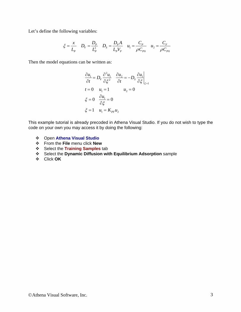
TTuuttoorriiaall:: DDiiffffuussiioonn iinn NNyylloonn--1122 FFoooodd PPaacckkaaggiinngg This example tutorial has been created to test the functionality of Athena Visual Studio in dealing with the solution of partial differential equations. An additional feature, the simultaneous solution of an ordinary differential equation, which is valid only on the right boundary is also demonstrated. The transport of a migrant from polymer to food is described by the following set of partial and ordinary differential equations:
2
2
0 0
0 0
P
P PP
F Pp
x L F
P Po F
P
P P PF F
C CDt x
C CDt x
t C C CCxx
x L C K C
υ υα α
ρ
=
∂ ∂=
∂ ∂∂ ∂
= − =∂ ∂
= = =
∂= =
∂= =
AV
We wish to solve for the concentration of the migrant in the food CF as function of time. Also we wish to plot the migrant concentration in the polymer CP as a function of time at different spatial locations. The values and description of the parameters for this process are given in the table below:
Model Parameters and Physical Properties Description and Units
This example tutorial is already precoded in Athena Visual Studio. If you do not wish to type the code on your own you may access it by doing the following:
Open Athena Visual Studio From the File menu click New Select the Training Samples tab Select the Dynamic Diffusion with Equilibrium Adsorption sample Click OK
IImmpplleemmeennttaattiioonn iinn AAtthheennaa VViissuuaall SSttuuddiioo The following step by step process describes the model implementation in Athena Visual Studio
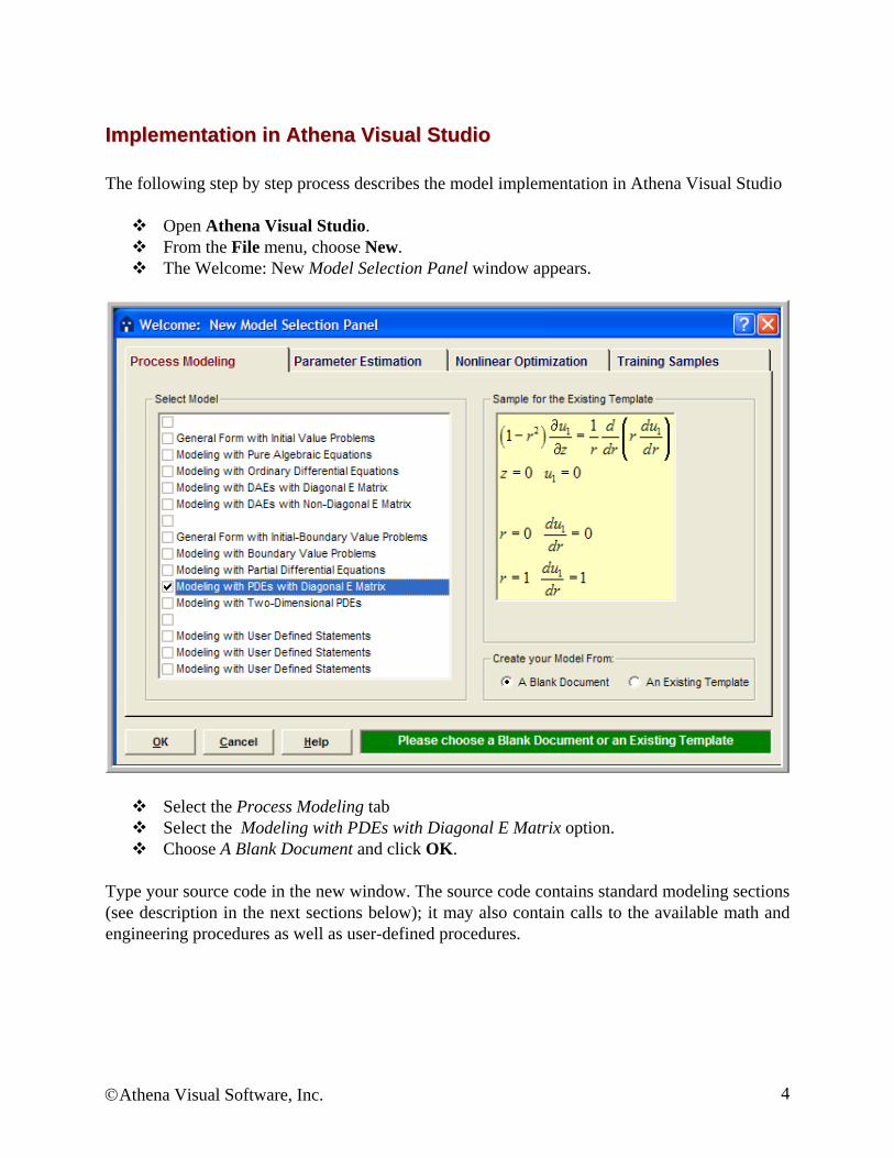
Open Athena Visual Studio. From the File menu, choose New. The Welcome: New Model Selection Panel window appears.
Select the Process Modeling tab Select the Modeling with PDEs with Diagonal E Matrix option. Choose A Blank Document and click OK.
Type your source code in the new window. The source code contains standard modeling sections (see description in the next sections below); it may also contain calls to the available math and engineering procedures as well as user-defined procedures.
WWrriittiinngg tthhee SSoouurrccee CCooddee You must enter a minimum of four sections in order to create the partial differential equations model with diagonal E( ) matrix. The first section labeled @Initial Conditions is used to insert initial values for the state variables vector. The second section labeled @Model Equations is used to enter the model equations. The third section labeled @Boundary Conditions is used to enter the boundary conditions. The fourth section labeled @Coefficient Matrix is used to enter the diagonal elements of the E( ) matrix. A data section not labeled by Athena Visual Studio may also be used to enter all the data pertinent to the model. The data section may also contain declaration statements for all model variables, parameters and constants. This section, if used, must be the first one in the model. The declaration of the model variables, parameters and constants must be done in accordance the Athena Visual Studio syntax rules shown below:
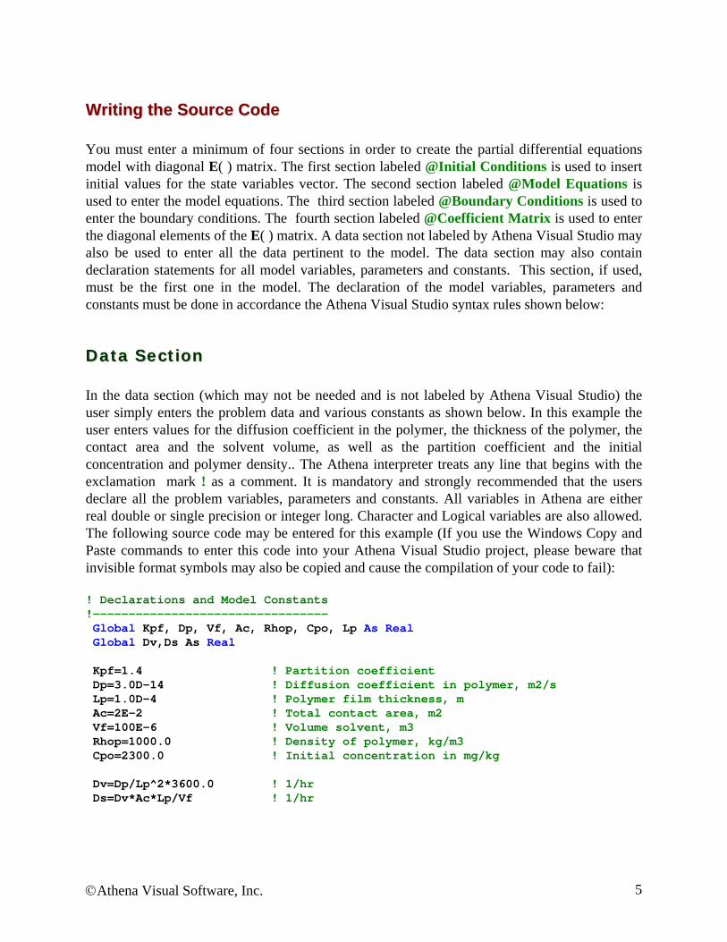
DDaattaa SSeeccttiioonn In the data section (which may not be needed and is not labeled by Athena Visual Studio) the user simply enters the problem data and various constants as shown below. In this example the user enters values for the diffusion coefficient in the polymer, the thickness of the polymer, the contact area and the solvent volume, as well as the partition coefficient and the initial concentration and polymer density.. The Athena interpreter treats any line that begins with the exclamation mark ! as a comment. It is mandatory and strongly recommended that the users declare all the problem variables, parameters and constants. All variables in Athena are either real double or single precision or integer long. Character and Logical variables are also allowed. The following source code may be entered for this example (If you use the Windows Copy and Paste commands to enter this code into your Athena Visual Studio project, please beware that invisible format symbols may also be copied and cause the compilation of your code to fail): ! Declarations and Model Constants !--------------------------------- Global Kpf, Dp, Vf, Ac, Rhop, Cpo, Lp As Real Global Dv,Ds As Real Kpf=1.4 ! Partition coefficient Dp=3.0D-14 ! Diffusion coefficient in polymer, m2/s Lp=1.0D-4 ! Polymer film thickness, m Ac=2E-2 ! Total contact area, m2 Vf=100E-6 ! Volume solvent, m3 Rhop=1000.0 ! Density of polymer, kg/m3 Cpo=2300.0 ! Initial concentration in mg/kg Dv=Dp/Lp^2*3600.0 ! 1/hr Ds=Dv*Ac*Lp/Vf ! 1/hr
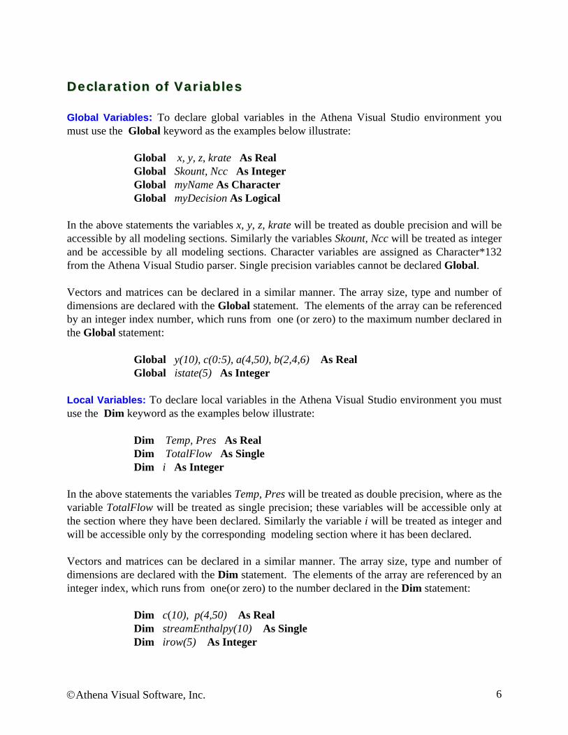
DDeeccllaarraattiioonn ooff VVaarriiaabblleess Global Variables: To declare global variables in the Athena Visual Studio environment you must use the Global keyword as the examples below illustrate:
Global x, y, z, krate As Real Global Skount, Ncc As Integer Global myName As Character Global myDecision As Logical
In the above statements the variables x, y, z, krate will be treated as double precision and will be accessible by all modeling sections. Similarly the variables Skount, Ncc will be treated as integer and be accessible by all modeling sections. Character variables are assigned as Character*132 from the Athena Visual Studio parser. Single precision variables cannot be declared Global. Vectors and matrices can be declared in a similar manner. The array size, type and number of dimensions are declared with the Global statement. The elements of the array can be referenced by an integer index number, which runs from one (or zero) to the maximum number declared in the Global statement:
Global y(10), c(0:5), a(4,50), b(2,4,6) As Real Global istate(5) As Integer
Local Variables: To declare local variables in the Athena Visual Studio environment you must use the Dim keyword as the examples below illustrate:
Dim Temp, Pres As Real Dim TotalFlow As Single Dim i As Integer
In the above statements the variables Temp, Pres will be treated as double precision, where as the variable TotalFlow will be treated as single precision; these variables will be accessible only at the section where they have been declared. Similarly the variable i will be treated as integer and will be accessible only by the corresponding modeling section where it has been declared. Vectors and matrices can be declared in a similar manner. The array size, type and number of dimensions are declared with the Dim statement. The elements of the array are referenced by an integer index, which runs from one(or zero) to the number declared in the Dim statement:
Dim c(10), p(4,50) As Real Dim streamEnthalpy(10) As Single Dim irow(5) As Integer
Parameter Statement: Use the Parameter keyword to define named constants as the examples below illustrate:
Parameter y=2.0, z=4.0 As Real Parameter Skount=1, Ncc=4 As Integer
In the above statements the variables y, z will be treated as double precision and their numerical values will be accessible by all parts of the modeling code. Similarly the variables Skount, Ncc will be treated as integer and their numerical values will be accessible through out all the modeling sections. The Parameter keyword is only allowed in the data section of the Athena Visual Studio modeling code. If it is used in the other modeling sections it will be ignored. You may view the generated Fortran code to see how the parser interprets the Parameter keyword. Important Note: Always remember to declare all of your variables. Athena treats Real variables as double precision, Integer variables as 4-byte integers, Character variables as Character*132 and Logical variables as .True. or .False. Single precision variables are only allowed if are declared as local with the Dim keyword. Fortran 95 Declaration Statements: You can insert Fortran 95 declaration statements by prefixing them with the double dollar sign. Below please see a list of Fortran 95 declaration statements that you can insert in your Athena code. Consult your Fortran 95 manual for the syntax rules of variable and constant declarations:
We are now going to describe in detail the various steps involved in writing the differential model for this example in the Athena Visual Studio environment. The modeling code is NOT case sensitive.
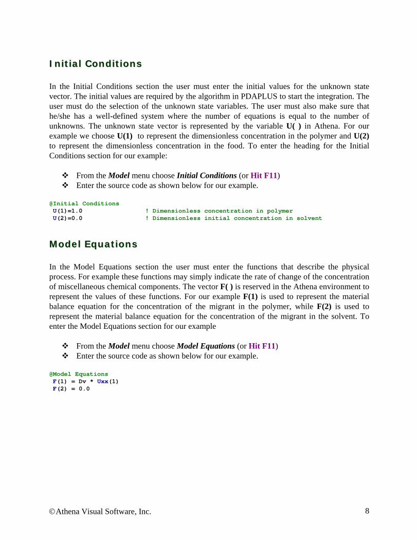
IInniittiiaall CCoonnddiittiioonnss In the Initial Conditions section the user must enter the initial values for the unknown state vector. The initial values are required by the algorithm in PDAPLUS to start the integration. The user must do the selection of the unknown state variables. The user must also make sure that he/she has a well-defined system where the number of equations is equal to the number of unknowns. The unknown state vector is represented by the variable U( ) in Athena. For our example we choose U(1) to represent the dimensionless concentration in the polymer and U(2) to represent the dimensionless concentration in the food. To enter the heading for the Initial Conditions section for our example:
From the Model menu choose Initial Conditions (or Hit F11) Enter the source code as shown below for our example.
@Initial Conditions U(1)=1.0 ! Dimensionless concentration in polymer U(2)=0.0 ! Dimensionless initial concentration in solvent
MMooddeell EEqquuaattiioonnss In the Model Equations section the user must enter the functions that describe the physical process. For example these functions may simply indicate the rate of change of the concentration of miscellaneous chemical components. The vector F( ) is reserved in the Athena environment to represent the values of these functions. For our example F(1) is used to represent the material balance equation for the concentration of the migrant in the polymer, while F(2) is used to represent the material balance equation for the concentration of the migrant in the solvent. To enter the Model Equations section for our example
From the Model menu choose Model Equations (or Hit F11) Enter the source code as shown below for our example.
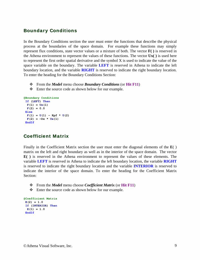
BBoouunnddaarryy CCoonnddiittiioonnss In the Boundary Conditions section the user must enter the functions that describe the physical process at the boundaries of the space domain. For example these functions may simply represent flux conditions, state vector values or a mixture of both. The vector F( ) is reserved in the Athena environment to represent the values of these functions. The vector Ux( ) is used here to represent the first order spatial derivative and the symbol X is used to indicate the value of the space variable on the boundary. The variable LEFT is reserved in Athena to indicate the left boundary location, and the variable RIGHT is reserved to indicate the right boundary location. To enter the heading for the Boundary Conditions Section:
From the Model menu choose Boundary Conditions (or Hit F11) Enter the source code as shown below for our example.
CCooeeffffiicciieenntt MMaattrriixx Finally in the Coefficient Matrix section the user must enter the diagonal elements of the E( ) matrix on the left and right boundary as well as in the interior of the space domain. The vector E( ) is reserved in the Athena environment to represent the values of these elements. The variable LEFT is reserved in Athena to indicate the left boundary location, the variable RIGHT is reserved to indicate the right boundary location and the variable INTERIOR is reserved to indicate the interior of the space domain. To enter the heading for the Coefficient Matrix Section:
From the Model menu choose Coefficient Matrix (or Hit F11) Enter the source code as shown below for our example.
@Coefficient Matrix E(2) = 1.0 If (INTERIOR) Then E(1) = 1.0 EndIf
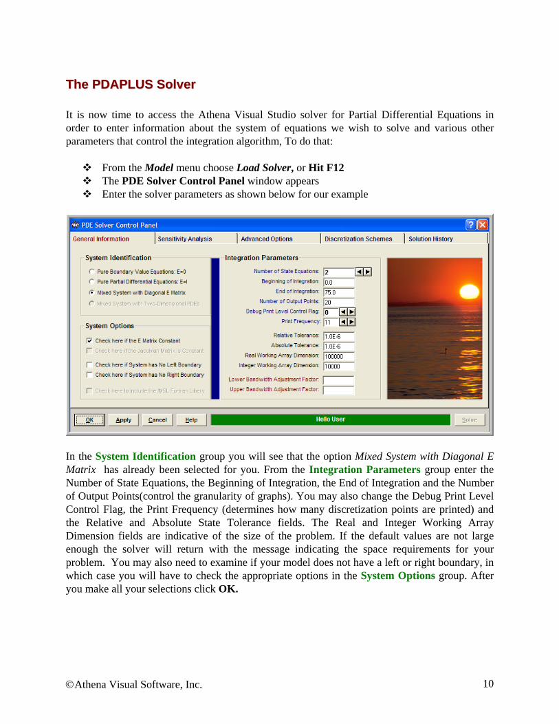
TThhee PPDDAAPPLLUUSS SSoollvveerr It is now time to access the Athena Visual Studio solver for Partial Differential Equations in order to enter information about the system of equations we wish to solve and various other parameters that control the integration algorithm, To do that:
From the Model menu choose Load Solver, or Hit F12 The PDE Solver Control Panel window appears Enter the solver parameters as shown below for our example
In the System Identification group you will see that the option Mixed System with Diagonal E Matrix has already been selected for you. From the Integration Parameters group enter the Number of State Equations, the Beginning of Integration, the End of Integration and the Number of Output Points(control the granularity of graphs). You may also change the Debug Print Level Control Flag, the Print Frequency (determines how many discretization points are printed) and the Relative and Absolute State Tolerance fields. The Real and Integer Working Array Dimension fields are indicative of the size of the problem. If the default values are not large enough the solver will return with the message indicating the space requirements for your problem. You may also need to examine if your model does not have a left or right boundary, in which case you will have to check the appropriate options in the System Options group. After you make all your selections click OK.
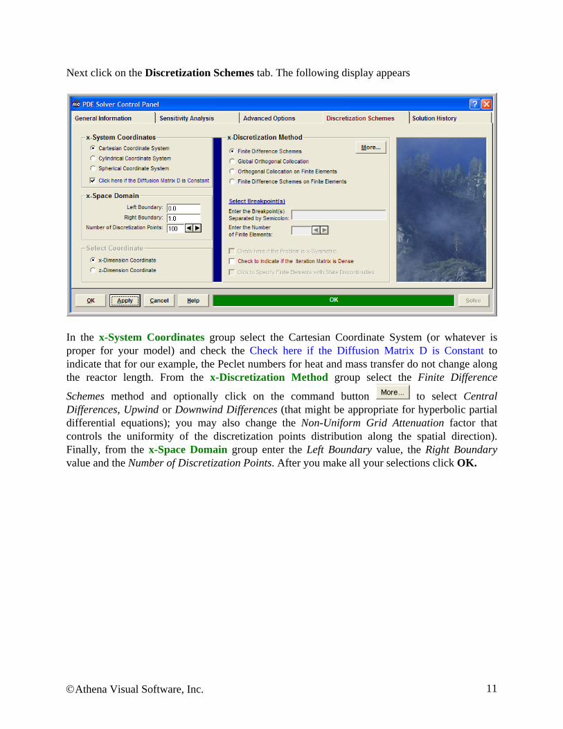
Next click on the Discretization Schemes tab. The following display appears
In the x-System Coordinates group select the Cartesian Coordinate System (or whatever is proper for your model) and check the Check here if the Diffusion Matrix D is Constant to indicate that for our example, the Peclet numbers for heat and mass transfer do not change along the reactor length. From the x-Discretization Method group select the Finite Difference
Schemes method and optionally click on the command button to select Central Differences, Upwind or Downwind Differences (that might be appropriate for hyperbolic partial differential equations); you may also change the Non-Uniform Grid Attenuation factor that controls the uniformity of the discretization points distribution along the spatial direction). Finally, from the x-Space Domain group enter the Left Boundary value, the Right Boundary value and the Number of Discretization Points. After you make all your selections click OK.
SSaavviinngg aanndd RRuunnnniinngg You are now ready to save your model and run it. New files are labeled UNTITLED until they are saved. Keep in mind that the maximum number of characters in a line is 132; the maximum number of lines in a file is infinity. In order to save your project:
From the File menu, choose Save. The Save As dialog box appears. This action saves your model and creates the Fortran code. In the Directories box, double-click a directory where you want to store the source file of
your project. Type a filename (a filename cannot contain the following characters: \ / : * ? “ < > |) in
the File Name box, then choose OK. The default extension is avw To view the Fortran code that you created from the View menu choose Fortran Code.
You may now choose to compile, build and execute your project; to do that:
From the Build menu choose Compile (or Hit F2) From the Build menu choose Build EXE (or Hit F4) From the Build menu choose Execute (or Hit F5)
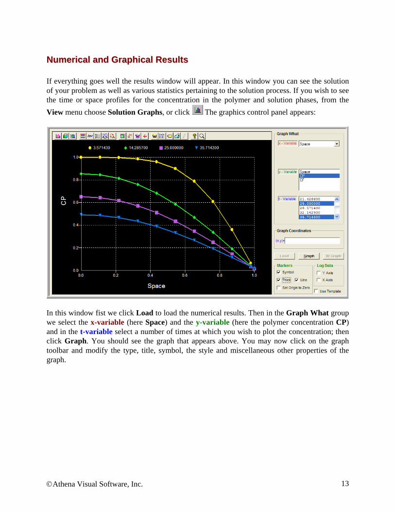
NNuummeerriiccaall aanndd GGrraapphhiiccaall RReessuullttss If everything goes well the results window will appear. In this window you can see the solution of your problem as well as various statistics pertaining to the solution process. If you wish to see the time or space profiles for the concentration in the polymer and solution phases, from the View menu choose Solution Graphs, or click The graphics control panel appears:
In this window fist we click Load to load the numerical results. Then in the Graph What group we select the x-variable (here Space) and the y-variable (here the polymer concentration CP) and in the t-variable select a number of times at which you wish to plot the concentration; then click Graph. You should see the graph that appears above. You may now click on the graph toolbar and modify the type, title, symbol, the style and miscellaneous other properties of the graph.
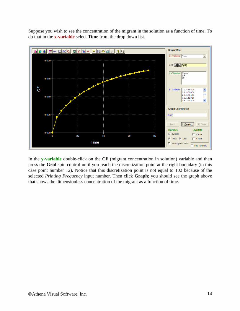
Suppose you wish to see the concentration of the migrant in the solution as a function of time. To do that in the x-variable select Time from the drop down list.
In the y-variable double-click on the CF (migrant concentration in solution) variable and then press the Grid spin control until you reach the discretization point at the right boundary (in this case point number 12). Notice that this discretization point is not equal to 102 because of the selected Printing Frequency input number. Then click Graph; you should see the graph above that shows the dimensionless concentration of the migrant as a function of time.
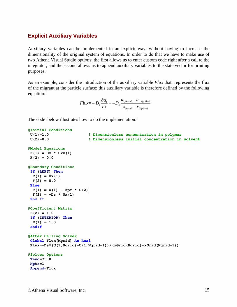
EExxpplliicciitt AAuuxxiilliiaarryy VVaarriiaabblleess Auxiliary variables can be implemented in an explicit way, without having to increase the dimensionality of the original system of equations. In order to do that we have to make use of two Athena Visual Studio options; the first allows us to enter custom code right after a call to the integrator, and the second allows us to append auxiliary variables to the state vector for printing purposes. As an example, consider the introduction of the auxiliary variable Flux that represents the flux of the migrant at the particle surface; this auxiliary variable is therefore defined by the following equation:
1, 1, 11
1
= Ngrid Ngrids s
Ngrid Ngrid
u uuFlux D Dx x x
−
−
−∂− = −
∂ −
The code below illustrates how to do the implementation: @Initial Conditions U(1)=1.0 ! Dimensionless concentration in polymer U(2)=0.0 ! Dimensionless initial concentration in solvent @Model Equations F(1) = Dv * Uxx(1) F(2) = 0.0 @Boundary Conditions If (LEFT) Then F(1) = Ux(1) F(2) = 0.0 Else F(1) = U(1) - Kpf * U(2) F(2) = -Ds * Ux(1) End If @Coefficient Matrix E(2) = 1.0 If (INTERIOR) Then E(1) = 1.0 EndIf @After Calling Solver Global Flux(Mgrid) As Real Flux=-Ds*(U(1,Ngrid)-U(1,Ngrid-1))/(xGrid(Ngrid)-xGrid(Ngrid-1)) @Solver Options Tend=75.0 Npts=1 Append=Flux
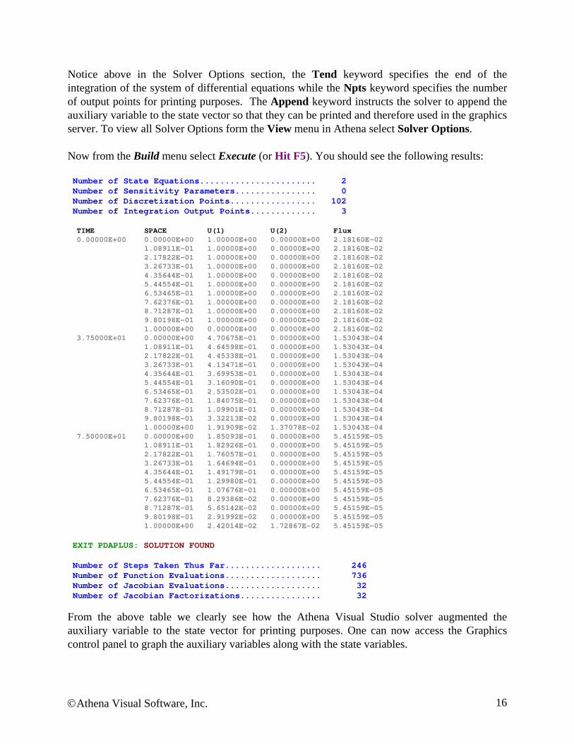
Notice above in the Solver Options section, the Tend keyword specifies the end of the integration of the system of differential equations while the Npts keyword specifies the number of output points for printing purposes. The Append keyword instructs the solver to append the auxiliary variable to the state vector so that they can be printed and therefore used in the graphics server. To view all Solver Options form the View menu in Athena select Solver Options. Now from the Build menu select Execute (or Hit F5). You should see the following results: Number of State Equations....................... 2 Number of Sensitivity Parameters................ 0 Number of Discretization Points................. 102 Number of Integration Output Points............. 3 TIME SPACE U(1) U(2) Flux 0.00000E+00 0.00000E+00 1.00000E+00 0.00000E+00 2.18160E-02 1.08911E-01 1.00000E+00 0.00000E+00 2.18160E-02 2.17822E-01 1.00000E+00 0.00000E+00 2.18160E-02 3.26733E-01 1.00000E+00 0.00000E+00 2.18160E-02 4.35644E-01 1.00000E+00 0.00000E+00 2.18160E-02 5.44554E-01 1.00000E+00 0.00000E+00 2.18160E-02 6.53465E-01 1.00000E+00 0.00000E+00 2.18160E-02 7.62376E-01 1.00000E+00 0.00000E+00 2.18160E-02 8.71287E-01 1.00000E+00 0.00000E+00 2.18160E-02 9.80198E-01 1.00000E+00 0.00000E+00 2.18160E-02 1.00000E+00 0.00000E+00 0.00000E+00 2.18160E-02 3.75000E+01 0.00000E+00 4.70675E-01 0.00000E+00 1.53043E-04 1.08911E-01 4.64598E-01 0.00000E+00 1.53043E-04 2.17822E-01 4.45338E-01 0.00000E+00 1.53043E-04 3.26733E-01 4.13471E-01 0.00000E+00 1.53043E-04 4.35644E-01 3.69953E-01 0.00000E+00 1.53043E-04 5.44554E-01 3.16090E-01 0.00000E+00 1.53043E-04 6.53465E-01 2.53502E-01 0.00000E+00 1.53043E-04 7.62376E-01 1.84075E-01 0.00000E+00 1.53043E-04 8.71287E-01 1.09901E-01 0.00000E+00 1.53043E-04 9.80198E-01 3.32213E-02 0.00000E+00 1.53043E-04 1.00000E+00 1.91909E-02 1.37078E-02 1.53043E-04 7.50000E+01 0.00000E+00 1.85093E-01 0.00000E+00 5.45159E-05 1.08911E-01 1.82926E-01 0.00000E+00 5.45159E-05 2.17822E-01 1.76057E-01 0.00000E+00 5.45159E-05 3.26733E-01 1.64694E-01 0.00000E+00 5.45159E-05 4.35644E-01 1.49179E-01 0.00000E+00 5.45159E-05 5.44554E-01 1.29980E-01 0.00000E+00 5.45159E-05 6.53465E-01 1.07676E-01 0.00000E+00 5.45159E-05 7.62376E-01 8.29386E-02 0.00000E+00 5.45159E-05 8.71287E-01 5.65142E-02 0.00000E+00 5.45159E-05 9.80198E-01 2.91992E-02 0.00000E+00 5.45159E-05 1.00000E+00 2.42014E-02 1.72867E-02 5.45159E-05 EXIT PDAPLUS: SOLUTION FOUND Number of Steps Taken Thus Far................... 246 Number of Function Evaluations................... 736 Number of Jacobian Evaluations................... 32 Number of Jacobian Factorizations................ 32
From the above table we clearly see how the Athena Visual Studio solver augmented the auxiliary variable to the state vector for printing purposes. One can now access the Graphics control panel to graph the auxiliary variables along with the state variables.