NASAReference

Publication1181

August 1987

Simplified Curve Fits

for the Thermodynamic

Properties ofEquilibrium Air

S. Srinivasan,

J. c. Tannehill,and K. J. Weilmuenster

Ig

https://ntrs.nasa.gov/search.jsp?R=19870016876 2018-06-11T16:44:34+00:00Z

ii i_

_ i_ ii_ _

NASAReferencePublication1181

1987

National Aeronautics

and Space Administration

Scientific and Technical

Information Office

Simplified Curve Fits

for the ThermodynamicProperties ofEquilibrium Air

S. Srinivasan

and J. c. Tannehill

Iowa State UniversityAmes, Iowa

K.j. Weilmuenster

Langley Research Center

Hampton, Virginia

Contents• , . • . .

At_st ra<'t ......

|ntrodnction .........

• , .

Behavior of Ah' at [tigh Temperature ......

Som'ces of Equilibrimn Air Properties ......• . .

Constructhm of Curve Fits .........• . , , . . . . . . . . .

Typical Cuw'e Forms ......

Transition Regions ......

Equation._ of the Curve Fits ...........• . , . , .

( ) .....p : p e, p . " "• , , , . , , ,

. -- .(e, I_I ..............• . • , , ,

T = T(_, p) ......... . .......

h = h(p, p) ......... . .....

T : T(I', P) ........... . .....• . . , . .

,_ = ,_(c,/_) ........ - • '• , .

p=p(P,'_) ......... . . .• . , . , .

c = _(p.._) ......... . .....• , . . .

. = _(/" '_) .........• • . . ,

t/esults and Conclusions .........

Appendix A Curve Fit Coefficients ........

p : p(_, P) ......... . ........... : .(_, _) ......... . .....

• . .

T : "I'(_, #) ........... . .....

h : h(p, p) ........... . .....

7"= "r(p,o) ............• . .

( ) .........,_; _ .,_ ¢. , p . , . . . .

p:#(p,.s) ......... . . .• . . . , ,

e = e(p, ,_) ........... . .....• . ° . . .

. = .(p, .) ........

Appendix B Master Program .....• . .

R(,fcrences ......

1

1

1

2

2

3

3

5

8

9

9

9

10

10

10

10

11

ll

11

26

26

26

26

26

26

26

26

26

26

43

44

oo*

LII

Abstract

New, improved curve fits for tile tlmrmodynamic

l)roI)erlies of equilibriunl air have been developed.

"File curve fits are for' pressure, speed of sound, ten>

perature, entropy, enthalpy, density, and internal en-

ergy. These curve fits can be readily incorporated

into new or existing computational fluid dynamics

codes if "real-gas" effects are desired. The curve fits

are constructed from Grabau-type transition func-

tions t.o model the thermodynamic surfaces in a

piecewise manner. The accuracies and continuity of

these curve fits are substantially improved over thoseof previous curve fits. These improvements are due

to the incorporation of a small nmnber of additional

terms in the approximating polynomials and care-

ful choices of the transition functions. The ranges

of validity of the new curve fits are temperatures up

to 25000 K and densities from 10 7 to 10a amagats.

Introduction

Under subsonic flight conditions, air may be

treated as an ideal gas composed of rigid rotating

diatomic molecules. The thermodynamic properties

of such a gas are well known. However, under hyper-

sonic flight conditions, air" may be raised to tempera-

tures at which the molecules can no longer be treated

as rigid rotators. Thus, there is a very real need for

the thernlodynamic and transport properties of equi-

librimn air for the computation of flow fields around

bodies in high-speed fight.. The references discussedbelow are representative of the various approaches

for obtaining t.hermodynamic properties, but the list

is by no means complete.

The thermodynamic properties of equilibrium

air were calculated with good confidence as early

as 1950. The earliest approach to compiling these

properties was to present the information in the form

of tables or charts (refs. 1 to 4).

Subsequently, equilibriunl air thermodynamicproperties became available inthe form of FOR-

TRAN computer programs. These programs can bebroadly divided into two categories. The first cat-

egory consists of programs that compute the equi-librium composition and thermodynamic properties

using a harmonic-oscillator rigid-rotator model for

the various component species of the gaseous mix-

ture. Programs (refs. 5 to 8) were developed for thecalculation of equilibrium properties of specific gas

mixtures or of arbitrary chemical systems.

The second category of computer programs, which

inchldes the present work, consists of programs that

determine the thermodynamic properties of equilib-

rium air in a noniterative fashion using either in-

terpolation or polynomial approximation techniques

(refs. 9 to 16). Typically, the sources of data for these

programs are references 1 to 4. One such program,

NASA RGAS (based on ref. 5), was an improvement

over other sources of t.hermodynamic properties in

terms of accuracy and range of validity. For this rea-

son it is still widely used. The major shortconfing of

the RGAS program is that the table lookup of coef-ficients for the cubic interpolation makes it. too cum-

bersome and time-consuming to be efficiently used

on an advanced computer.

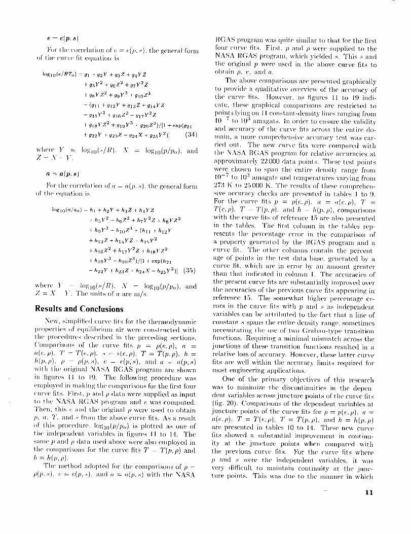
Tannehill and associates (refs. 10, 15, and 16) de-

veloped simplified curve fits for the thermodynamic

and transport properties of equilibrium air with thesame range of validity as the NASA RGAS program.

The curve fits were constructed through the use of

Grabau-type transition functions in a manner sim-

ilar to that of reference 11. In forming these curve

fits, as many as five Grabau-type transition flmctions

were joined with the perfect-gas equation of state.

One of the major shortcomings of the curve fits

of references 10, 15, and 16 is the lack of continuityacross the boundaries between the transition func-

tions. As a consequence, numerical difficulties weresometimes encountered when these curve fits were

employed in iterative flow-field computations. The

primary objective of the present research was to al-

leviate this difficulty. At the same tilne, an attempt

was made to improve the accuracy of the curve fits

through incorporation of a small number of addi-

tional terms which would not significantly increasethe computation time.

Through careful choice of the Grabau-type tran-

sition flmctions and use of complete bicubic polyno-

mials, curve fits for pressure, speed of sound, temper-

ature, entropy, enthalpy, density, and internal energy

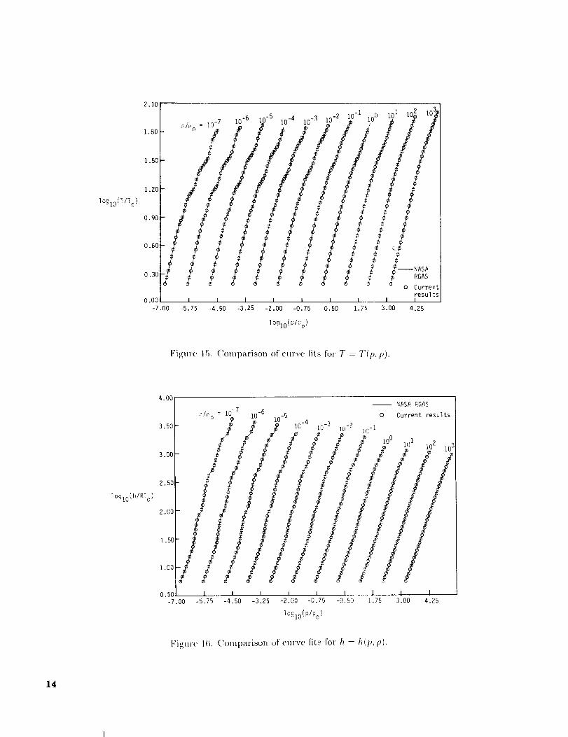
were developed and are presented herein. Thesecurve fits are based on the NASA RGAS data and

have the same ranges of validity, namely, tempera-tures up to 25000 K and densities from 10 -7 to 103

amagats (P/Po).

Symbols

a speed of sound, m/s

e specifc internal energy m2/s :a

h specific enthalpy, m2/s 2

p pressure, N/m 2

R gas constant, 287.06 m2/s2-K

s specific entropy, m2/s2-K

T temperature, K

=

p density, kg/m:"

Subscript:

o reference con(litions at 1 arm and

273.15 K

Behavior of Air at High Temperature

When a gas composed of polyatomic molecules is

healed to high t enlperat.ures, its conlI)osit ion changes

as a result of the chemical reactions which take place.Sucll a situation exists behind the shock wave which

enw'tops a vehicle entering the atmosphere of the

Earth. As a result of the change in chemical com-

position, the thermodynanfic properties of the gas

also change. When the temperature of tile gas is

raised apl)reciably higher than ,the temperature atwhich dissociation reactions begin to occur, the elec-

trons receive energy quanta because of tile collisions

between atoms. If the temperature, and hence the

kinetic energy of the atoms, is high enough so thatelectrons are removed from their orbits, ionization of

the gas takes l)lace. The eft'cots of dissociation andionization of the gas on its thermodynamic properties

are often retk'rred to as "real-gas" efl)cts.

At room temperature, the volumet ric composition

of air is about 78 percent diatomic nitrogen, 21 per-cent diatomic oxygen, an(t about 1 t)ereent argon

and tra('esofcarbondioxitte. When the temperature

of air is raised above room temperature, deviations

from perfect-gas I)ehavior occur; thai is, the vibra-tional mode of the molecules becomes excited, disso-

ciation of both oxygen and nitrogen molecules occurs

(although at different temperatures), nitric oxide isfornw(t, and so forth. The chemical composition of

air for densities lying between l0 2 and 10 times nor-

real air density is approximately divisit)le into the

following regimes:

1. T < 2500 K. The chemical coInt)osition is sub-

stantially that at room temperature.

2. 2500 < T < 4000 K. This is the oxygen (tisso-

elation regime; no significant nitrogen dissoeia-ti(m occurs; some NO is formed.

3. 4000 < T < 8000 K. This is the nitrogen dis-

sociation regime; oxygen fiflly dissociates.4. T > 8000 K. Ionization of the atomic

constituents occurs.

Sources of Equilibrium Air Properties

The following discussion is intended to summarize

the availat)le nmchanisms for determining equilib-rinm air properties. The cited references are not in-

tended as a complete compilation but serve only as a

list lug typical of lhe various methods for determining

tile properties.

Prior to 1.961). methods for determining equilib-

rimn air 1)rOl)erlies were available only in summaryform as tables or charts. The sources for information

were the calculations of Gihnore (ref. 1}, Hilsenrath

and Beckett (re['. 2), Hansen (ref. 3), and Moeckel

and Weston (rcf. ,1). In reference 3, data for com-

pressit)ility factor, ent.halpy, speed of sound, sl)ecificheal, Pran(ltl mlluber, and the coefficients of viscos-

ity and conductivity are presented as functions of

temperature and t)ressure.

Evemually, the calculation of equilibrimn air

properties was possible through the use of FOR-

TRAN computer programs, which can be divided

broadly inlo two categories. The first category

consists of programs that compute the equilibrium

COml)ositi()n an(I lhermo(lynamic properties using a

harmonie-oscilhm)r rigid-rotator model for the vari-

ous comp(ment _l)ecies of the gaseous mixture, llai-

1CV (ref. 5) developed computer t)rograms whichused the teniperature, density, an(t molar co1R:en-

trations of the various constituent species to calcu-

late the pressure, gas constailt, ent.halpy, entrol)y,

specific heats, and coefficient of thermal conductiv-

ity. These prol)erlies were computed for a 9-speciesmodel as well as an 11-species model of equilibrium

air. Zeleznik aH,l Gordon (ref. 6) (teveloped a so-

phisticated computer program, improved later by

Gordon and McBri(te (ref. 7), which computed the

chemical e(luilil_fium composition of complex chemi-

cal systems given the constituent species and one of

five possit)h, pairs of thermodynamic state coml)ina-

tions. Also. a 27-reaction equilil)rium air program

was developed by Miner et al. (ref. 8).

The secured category of computer programs con-

sist.s of programs lhat determine the thermodynanfic

properties of equilibrium air in a noniterative fashion

using either ot' lhe interpolation-of-polynomial ap-

proximatio_ techniques. Lomax and Inouye (ref. 9)

developed F()I{TIIAN t)rograms to determine the

speed of sound, emhalpy, temperature, and entropy

as functions of either pressure and density or pres-

sure and et,tr(_tLv. Tileir programs used a 9-point

spline interpolalion and required a lookup of over

10 000 tabulated values. The programs developed atNASA Ames Research Center in reDrences 5 and 9

eventually evolved into the NASA RGAS program.

The NASA I{(;AS t)rogram employs a cubic inter-

polation technique, with the associated table lookup

of cubic coeflMents, to compute tile enthalpy, ten>t)erature, ent,'op._, and speed of sound of 13 different

gas mixtures, including equilibriun_ air as functions

of either pressure and density, or pressure and en-

tropy. The N.,k%.\ RGAS program was n_o(tifie(l t)y

Zammhill and Mohling (ref. 10) to allow internal en-

ergy and density Io be used as independent variables

for "time-dependent"flowcalculations.Themajorshorlcomingof the I{GASprogramis that tire ta-blelookupof co(,tticientsfor the cubicinterpolationmakesit IooClllll})ersoilleall(t time-consuming to be

efficiently employed on an advanced computer.

AlllOr|g Ill(' tirst to develop programs which

at)proximate(] lhe thermodynamic properties

as self-contained closed-form expressions was

(;ral)au (ref. 11). tie outlined a systematic tech-

ni(tue of mo(leling the thermodynamic properties

with polynomial expressions containing exponential

transitions. Using this technique, tledetermine(ltheOlll hall)y, entropy, speed of sound, and compressibil-

ity of equilil)rhml air as functions of l)ressure an(t

density in the form of closed-form expressions (curvefits). [_sing (;rabau's technique, Lewis and Burgess

(ref. 12) obtained emt)irical equations for the density,

enthalpy, sl)ee(l of sound, and compressibility factor

of air as time(ions of pressure and entropy. How-

ever, these curve fits had a range of vali(lity only up1.o 15000 K and a pressure range of 0.1 to 1.0 atm.

The method of reference l l was also employed by'

P,arnwell (ref. 13) to curve fit _ as a flmct.ion of in-

lernal energy and density and temperature as a func-

tion of pressm'e and density for equilil)rium air. Vie-

gas and Howe (rcf. 14) (levcloped programs for the

density, temperature, viscosity, and Pran(ltl nmnber

of equilibrium air as functions of pressure and en-

thalpy ill the form of curve fits using least squaresan(t Chet)yshev polynomial fitting. Tannehill and

associates (refs. 10, 15, and 16) developed simpli-

fie(t curve fits ['or lhe thermo(lynanlic and transl)ort

pr(iperties of equitil)rimn air with the same range of

wdi(lity as the NASA R(IAS program. These curve

fits included pressure, temperature, speed of sound,

and coelficients of viscosity and thernla] conductivityas funct.ions of internal energy and density; also in-

cluded were temperature an(l enthalpy as fimctions of

pressure an(t density. The curve fits were constructedusing Gral)au-type transition time(ions in a manner

similar to that of reference l l. In forming these cm'vefits, its many its five Grabau-type transition functions

were joined with tilt, perfect-gas equation of state.

Construction of Curve Fits

Typical Curve Forms

In tire flow calculations of air in thermody-

nanlic equilibrium, it. becomes important to knowthe wtrious thermo(tynamic properties as functions

of a l)air of in(lepen(lent state variables. In or-

der to illustrate the spatial behavior of these t.her-

mo(tynamie surfaces, a typical curve is examine(there ill some (telail. Tlle nature of the thermo-

dynamic srlrface, with the plausible reasons for its

undulating behavior, provides a qualitative insight

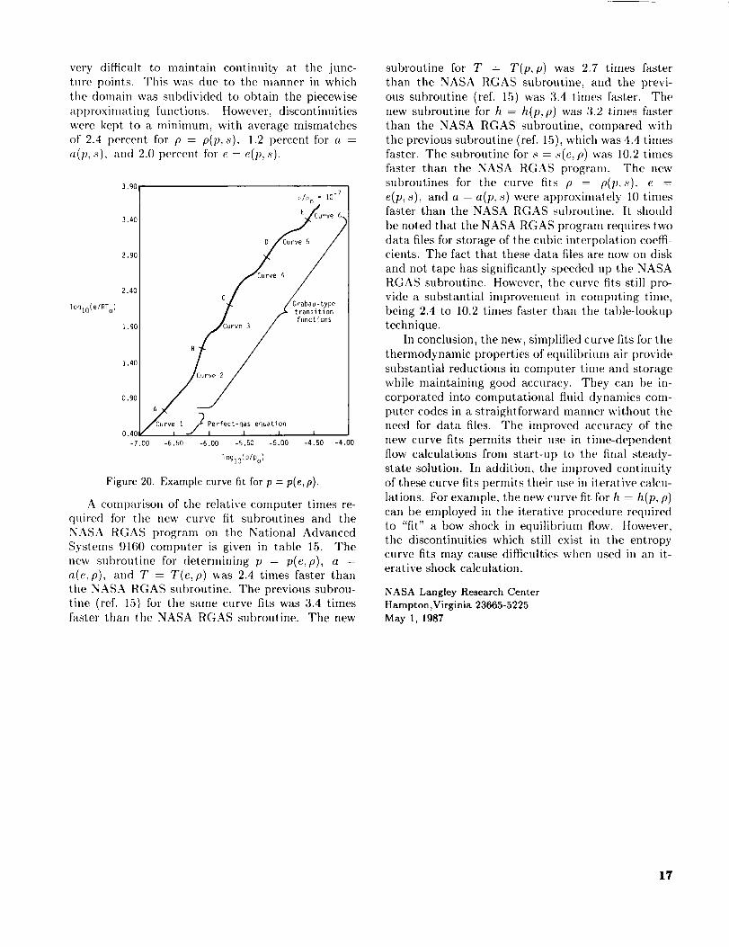
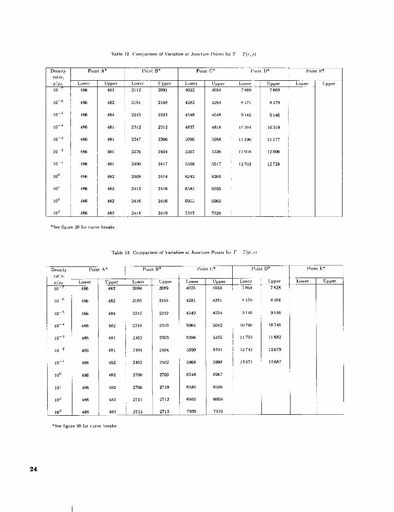
into the choice (if the al)l)roximating flmctions. Fig-ure 1 shows the function "} plotte(t with respect to

loglo(p/po) - logm(p/po) at a density of 10 -7 ama-

gats. Also shown are tile various segments into which

the curve may be divide(t, as indicated by A, AA, B,

C, and D. These segments are basically quadratic or

linear curves which are joined together I)y transition

curves. Two tyl)es of transition curves al)pear in fig-

ure l, and these are illustrated ill figures 2 an(t 3.

Figure 2 shows a transition flmction which passesthrough a point of inflect.ion and is referred to as a

transition wit, h inflection. Figure :3 illustrates the sec-

ond type of transition, which is one without a point

of infleetiom Figure 1 shows that _ goes through

three distinct transitions with inflections. Accordingto reference 3, there is a definite correlation between

these three transitions and the change in chemicalcomposition of the air" as the temperature increases:

the first transition, from AA to B, is due to the oxy-gen dissociation reaction; the second, fl'om B to C,

is due to the nitrogen (lissocialion; and the third,from C to D, is due to the ionizat.ion reactions.

In addition to the three transitions with inflec-

tions in figure l, there appears to be a relatively in-

significant transition without an inflection between

curves A and AA. Also, after" a careflil examination

of segment D, it appears that it may actually I)e part

of an incomplete transition with a point of inflection.

Tile t.erm _, is plotte(t as a function of loglt)(p/po)-

loglo(p/p,, ) for various densities in figure 4, which

includes the cm've fit. of figure 1. As the density

increases, pieces of the curve near C an(t D disap-[)eat" tmtil only a part of the transition into C re-

nlains at 10a amagats. The reason for this is that the

compressibility factor decreases steadily as tile den-sity is increased isothermally. Itence, it also follows

that isothermal points move rapidly along the curve

from D toward C as the density increases. Figure 4

provides an idea of tlle complexity of the problem of

devising a practical method of modelling the collapse

of the lower segments with increasing density. There

appears t.o be a tendency for transitions with inflec-tions to convert to transitions without inflections as

the density increases. Reference 1 suggests that this

conversion might be correlated with the simultane-ous, abrupt increases of the concentrations of ionized

oxygen an(t nitrogen atoms and of ionize(t nitrogenmolecules.

As a consequence of the above (tiseussion, one

is motivated to model the thermodynamic surface,

in a piecewise manner, with biquadratic or bicubic

polynomials joined together by exponential transi-

t.ion functions with or without points of inflection.

This is tile procedure adopted in the l)resent study.

3

i .40

1.35

1.30 -

i .25 -

-7

i .20 -

1.15 -

1.10 -

i .05

0.00

AA

B

P/PO =

I [ I I I i I

0.40 0.80 1.20 1.60 2.00 2.40 2.80

loglO(p/po ) - loglo(C/Oo )

Figure 1. Variation ot_,, with logio(p/po) - logl0(/,/P.) f'o,' t'/Po = 10-7

10-7

3.20

amagats.

fl (x)

Figure 2. Transition curve with inflection.

f2 x)

fl(x)

Figure 3. Transition cm've without inflection.

Transition Regions

The bask: fornls of the variables _ and lOgl0(T/To),

plotted at eonstam, densities as functions of

lOgl0(p/po ) -logl0(p/po), are shown in figures 4and 5. As mentioned previously, these curves ex-

hibit segments of linear or quadratic functions suc-

cessively connected by transition fimctions, which

are asymt)totic at both ends, attd may or may not

include points of inflection. The fact that at least,---;()nleof these transitions can be attrit)uted to dis-

sociation phenomena suggests the use of exponentialdistribution functions.

Following the method outlined by Grabau (ref. 11),one has a choice of two kernel transition flmctions.

The first is the Fermi-Dirac fimction

1 + exp(kx)(1)

which represents a transition between the levels zero

and ,ratty, where the direction and rate of the transi-

tion depend on the sign and tile nmnerical magnitude

of the exponential constant k. The numerator defines

the upper level of the transition and may take on a

variety of forms. In tigure 6 the Ul)t)er level of the

transition is a straight line inclined to tile horizontal,while the lower level is the z-axis. The transitions in

tigure (i have points of inflection and, in the termi-

nology of Gral)au (ref. 11), are referred to as oddtransitions.

The second type of transition fimction is thekernel of the Bose-Einstein distritmtion function

1 - exp(kx)(2)

which provides transitions leading from one function

to another without a point of inflection and is ob-

tained by merely changing the sign before the expo-nential term in the ¢tenominator of the Fermi-Dirae

function. The transition function given by equa-

tion (2) is termed an even transition. Figure 7 illus-trates two transitions of this kind between the x-axis

and the line y = z, where (as before) the directions

and rates of the transitions are governed by tile sign

and magnitude of tile exponential constant k. It is

imt)ortant to note that the expression for an eventransition becomes an indeterminate form when x is

equal to the z-coordinate of the point of intersectionof lhe two lines t)ounding the transition.

In the current study, each of the thermodynamic

curves is approximated with quadratic or incomplete

cubic segments connected by odd and even transi-

tions as described above. Ahnost without exception,

at tow densities all the curves undergo odd transitions

which gradually diminish as the density increases and

then change to even transitions. There are two waysof applying each of these transition fimctions. When

the path of a curve appears t.o move from one straight

line to another, there is an offset, present which canbe calculated in the direction of either of the vari-

ables. For accuracy it appears to be better to viewthe transition in terms of the smaller offset. Both

ways of viewing the offsets involve the choice of a

baseline. Tile use of the offset in tile g-direction sim-

plifies this choice since the x-axis serves as a naturalbaseline.

Consider the problem of determining the equation

of a curve consisting of two linear segments connected

by' an odd transition fimction (fig. 8). Tile lower and

upper line segments are given by

y, = alx + b! (3)

and

Y2 = a2x + b2

The y offset is their difference:

(4)

Y2 - Yl = (a2 - al)x+(b2 - bl) (5)

which becomes the numerator of the transition flmc-

tion. The remaining constants of the transition func-

tion can be found graphically by drawing three lines

t)etween Yl and Y2. The median line is given by

Yl +Y2Y"-- 2 (6)

Let Ya be the median line between Yo and Yl and Yb

be the corresponding median line between Yo and Y2.

The center of the transition, (zo, Yo), is the point at

which the transition crosses tile median line Yo. Thedesired transition function is then of the form

(a2 - al)x + (b2 - bl)

Y = Yl + 1 + exp[k(x - xo)] (7)

The exponential constant k is found from the coor-

dinates za and z b at which the transition intersects

the lines Ya and Yb. Specifically, for the intersection

with the line 9a,

1 1(8)

1 + exp[k(za - Xo)] = 4

so that

exp[k(xa - Xo))= 3

SoMngfor k yields

(9)

k __

In 3

Z a -- Z o

1.401

1.35

O-0.5

1.25\

....ii:i

t ---- -4.5

1.10 F/

1.05 I I I I I I I0.00 0.40 0.80 i .20 i .60 2.00 2.40 2.80 3.20

loglO(p/po) - lOglo(C:/%)

Figure 4. Variation (d"_ with logH)(p/t_, ) loglO(p/p, ) for various densities.

lo910(T/To )

2.10 _/c_ = 103 //

/ /10 -4.5

lo1.80 '.-/

1.50

1.20

0.90

0.60

0.30

O.OC

i0-0"5

1 I I I ! I I

0.00 0.40 0.80 1.20 1.60 2.00 2.40 2.80 3.20

lOglo(p/po) - ]Oglo(P/c o)

Figure 5. Variation of logl0(T/T,, ) with logl0(p/p_, ) logics(/,/p,, ) for various densities.

6

i .00

0.75

0.50

0.25i

0.00

5x=-. + 0.75

_"" y = 0.0

-0.25 i l i i J ! i !

-i.00 -0.80 -0.60 -0.40 -0.20 0.00 0.20 0.40 0.60 0.80

Figure 6. Two odd transition functions.

2.00

1.50

i .00

O. 50

0.00

-0.50

-2.00

y =

x Y x. 1 -

___17/ y : o o

F_ X

I I I I I-1.50 -i.00 -0.50 0.00 0.50 1.00 1.50 2.00

Figure 7. Two even transition functions.

20.00

17.50

15.00

12.50

i0.00

7.50

5.00

2.50

0.00

-2.5C-5.0

Y

Yb

Yo

Y I i a

I I It I

I t IIX IX Ix

Xo xbI ; i II I

0.00 5.00 10.00 15.00

Figure 8. Construction of an odd transition function.

Fronltile intersectionof y with Yb we get

In 3# - (11)

2"o -- 3"b

This procedure obviously yields two numerical values

for the constant k. However, they are substantiallyalike in most instances.

The (letermination of the constants of an even

transition is simpler. In terms of the !i offset, such atransition can be written in the form

.(:_ -..)g = 1 - exp[k(x -.r.)] (12)

where .re is tile x-coordinate of tim point of intersec-tion of the two lines bounding the transition. The

value of the exponential constant /,' follows from the

coordinate .qo at x = Xo. Since the expression for y is

an indeterminate form at this point, its value is givenby the ratio of the derivatives of the nmnerator and

of the denominator at this point:

= (13),qo .r lira ---+ :ro

which gives

/,-= -- (14),qo

This approach for determining the constantsof the Grabau-type transitions is extended in the

present work to approximate transitions in two in-dependent variables. The kernel of an odd transitionfunction in three dimensions is

1 + exp(ao + aim + a2g + a3rg)(15)

which is essentially an alternate form of

1 -+-exp[k(x - xo)(g - y,,)](16)

Equation (15) is more convenient for determining the

values of the constants a0 to a3 as dictated by thebehavior imposed on the transition function. The

general technique of determining t he values of these

constants differs from the approach outlined earlieran(t is as follows. The boundaries of the transition in

the (tirections of the two indepen(ten! variat)les are

x,, < x < ,rb an(t gc <_ y <_ Yd. If fl (x, y) and f2(x, y)

are the two surfaces limiting the transition functionf(x, .q), then

f(x,y) = fl(w,y) + f2(x,y) - fl(x,y) (17)1 + exp(ao + alx + a2g + a3xy)

In order to ensure an accurate and smooth transition

from fl(x,g) to f2(x,9), we require the quadratic

expression (% 4 alZ + a2y + a3xy) to behave as

follows. At the lower left corner point (xa,yc) the

quadratic ext)ressi(m should have a large positive

vahte so that f(,,', y) _ f,(z, g). At the upper right

corner point (.rh, !l,I) the quadratic expression shouldhave a large neg_tlive value in order to ensure that

f(x,g) _ f2(.r,y). At the midpoints of the left

and right boundaries, [xa, (Ye + Yd)/2] and [Xb, (Yc +yd)/2], respect ixely, the quadratic expression shouldbe zero so lhat

f( u] + f2(_,y)f(.r,9) _ ,l,x,o,

2

These conditions yieht tile following four linear equa-tions:

al) + a l.ra + a2gc + a3xagc = +k (18)

(q) + ¢*l.rb + a2Yd + a3xbYd = -k (19)

a0+al,r,+a2(.q,. +-.qd)/2+a3xa(yc+yd)/2 = 0 (20)

a0+olxt,+a2(,q, +-gd)/2+aaxb(Y,.+yd)/2 = 0 (21)

where k is a positive constant (typically 20 < k < 25)

chosen such that exp(k) and exp(-k) do not. yield

overflow and underflow conditions on a computer.The constants a0 to a3 can now be obtained in

a straightforward manner from the system of four

linear equations in four unknowns (eqs. (18) to (21)).

The above met hod of obtaining tile Grabau-type

transition functions proved quite accurate in ensur-

ing a negligible mismatch in the dependent variable

over the boundarie.s of adjoining subregions. It. is amerit of this stepwise method of constructing em-

pirical equations that any part can I)e removed for

corrections without disturbing the surface approxi-mation as a whole.

Equations of the Curve Fits

The curve Iris for the various thermodynanfic

properties are constructed through use of Grabau-

type transition functions, as described previously.The general form of these curve fits can be writtenas

z(x,y) = fl(x,g) + f2(x,y) - f,(z,y) (22)1 ± exp(k 0 + klx + k2y + k3xy)

where, in general,

f_ (x, y) = Pl + P2 :r + PaY + p4xy + p5 x2 + p6y 2

+ p7:r2Y + p8xy 2 + p9 x3 + ploy 3 (23)

alld

f2(x,y) -- fl(x,y) = Pll +Pl2 x + pl3y + Pl4Xy

+P15 x2 +Pl6Y 2 +PlTx2y

+ plsxy 2 + p19 x3 + p20y 3 (24)

The coefficients k0 t(i ka in tile denonlinator of the

lransition function in equation (22) are (tetermined

l)y the technique outlined in tile preceding section.

The coefticients #q t(i P20 in equations (23) and (24)

are determined by the actual curve fitting of the data

froni the NASA R(,AS l)rogram. The exact location

aml mlml)er of these data points over the cm've fit

(I(imain deternlines the accuracy of the curve fits.

The I)oints are clustered near the boundaries of the

domain and the nliddle region of the transition in

order to ensure continuity at the boundaries aimaccuracy within the domain, The data from the

NASA RGAS program are fitted to the equations

of the curve fits t)y the method of least squares. A

multiple linear regression technique (ref. 17) is used

t(/ determine the coetficients P l to P2(}.

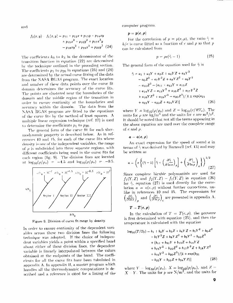
The genera[ form of the curve fit for each ther-

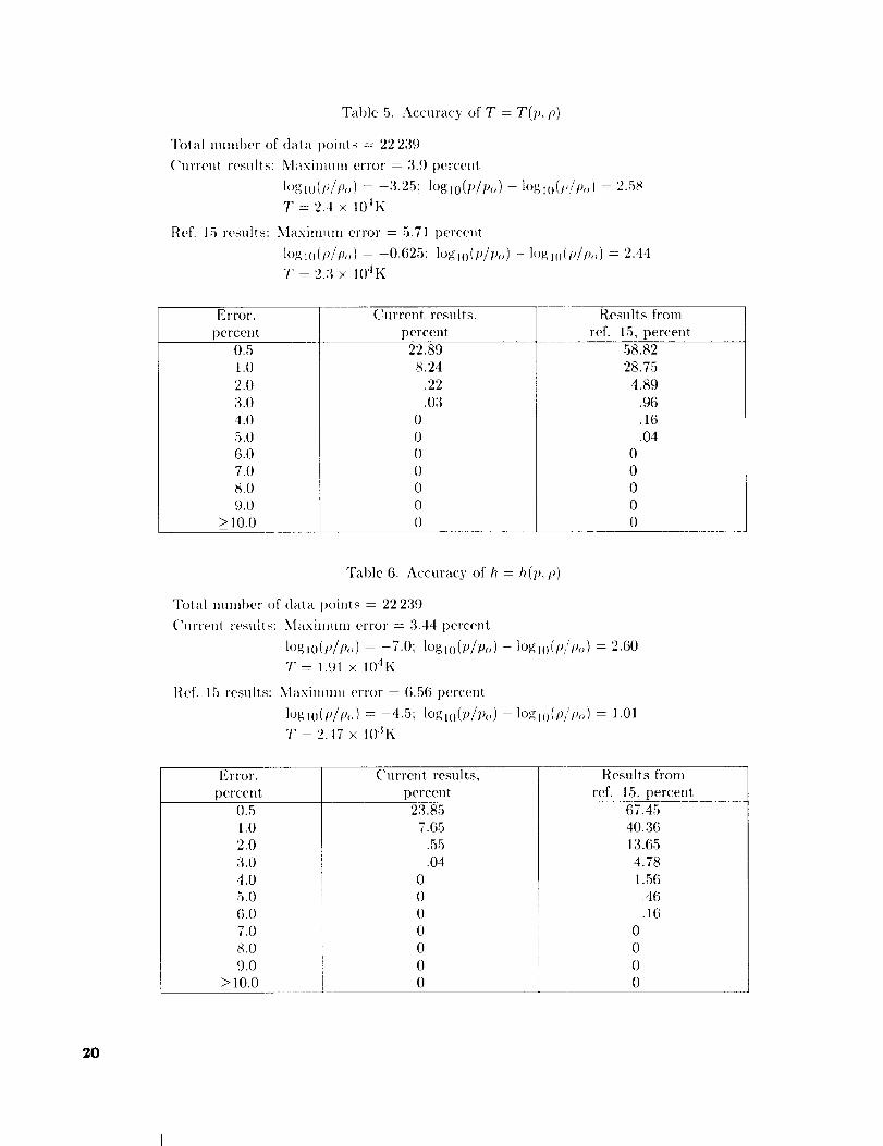
modynamic property is described below. As in ref-eren('es I0 an(1 15, for each of the curve fits where

(tensity is one of the independent variables, the range

(if p is sub(livi(le(l into three separate regions, withdifferent coefficients being used in the curve fits for

each regi(ln (fig. 9). The division lines are located

at I(igl()(p/a<, ) = -4.5 and loglo(p/p<, ) = -0.5.

h/h o

P/Po

Figure 9. Division of curve fit range by density.

In order to ensure continuity of the dependent vari-

allies across these two division lines the following

technique was adopted. If the choice of indepen-

(lent variables yields a point within a specified band

about either of these division lines, the dependent

variable is linearly' interpolated between the vahles

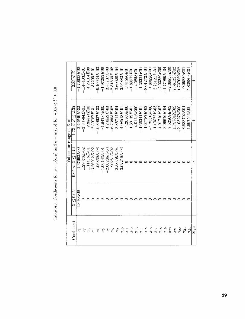
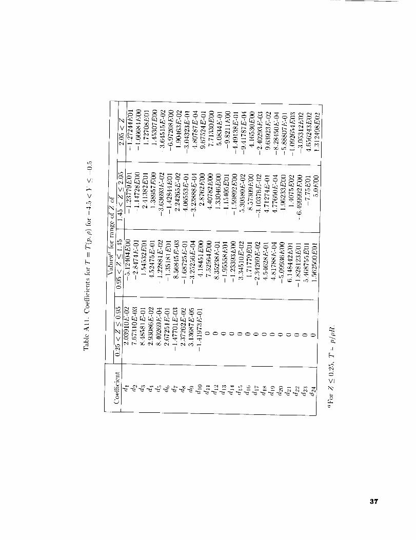
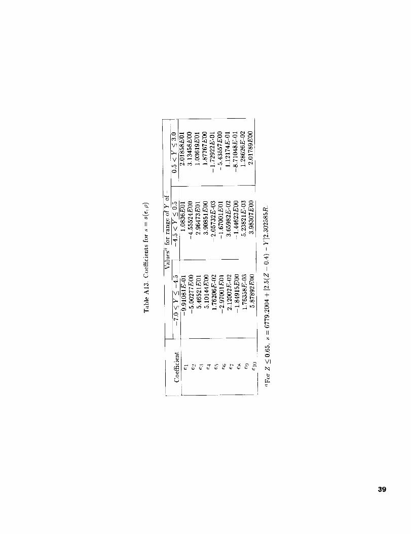
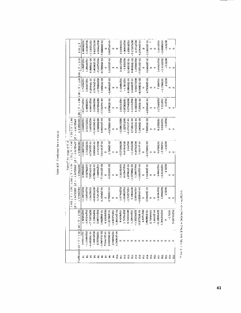
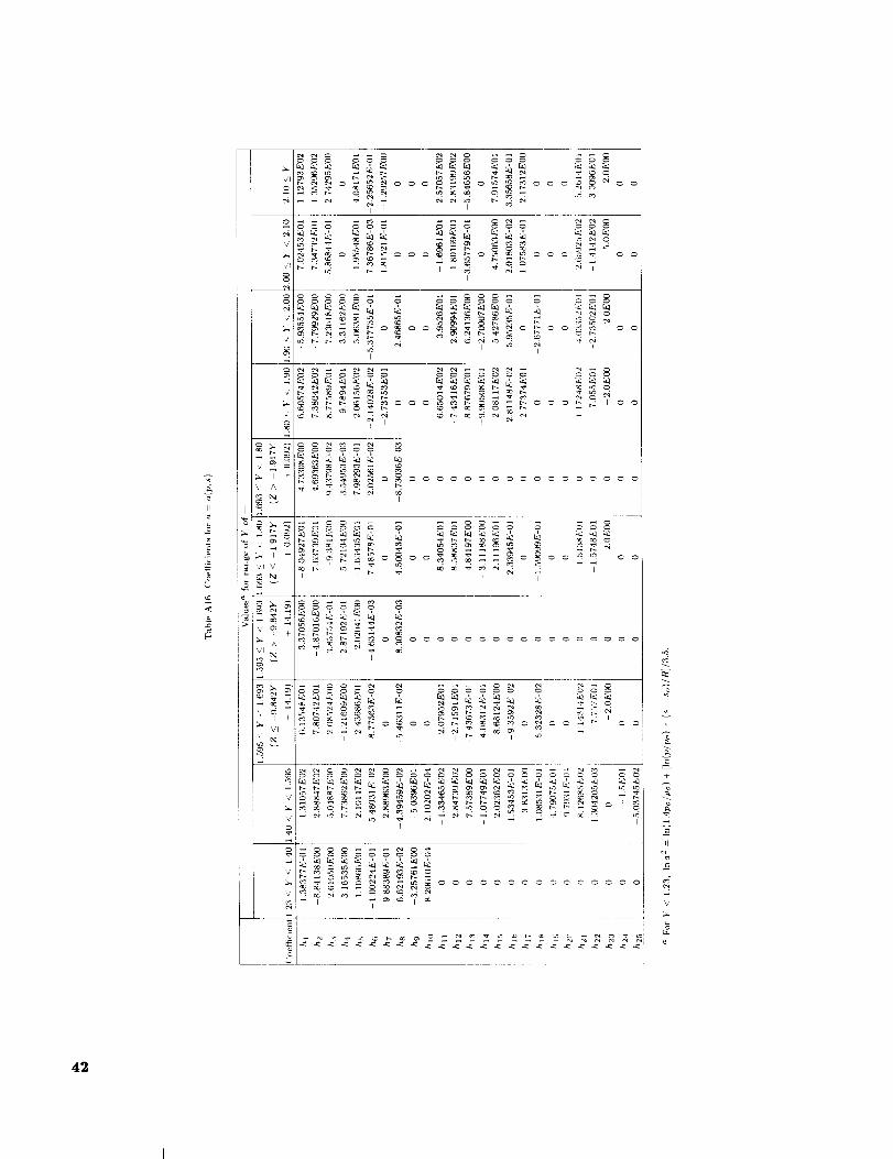
obtained at the endpoints of the band. The coeffi-cients for all tile curve fits have been tabulated in

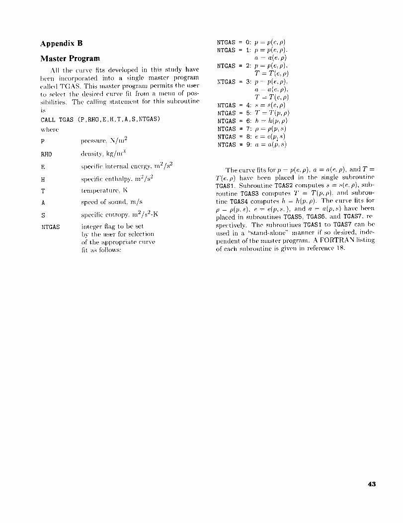
al)pendix A. In appendix B, a master progranl which

handles all the thernlodynamie computatiolls is de-

scribed and a reference is cited for a listing of the

computer progranl.

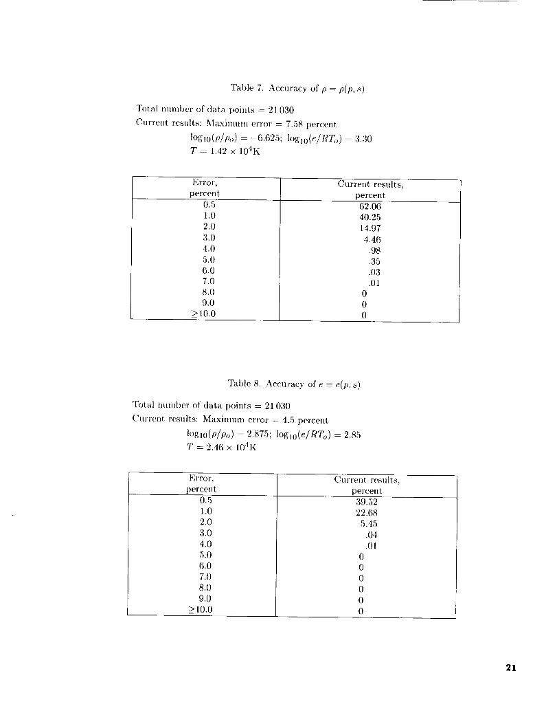
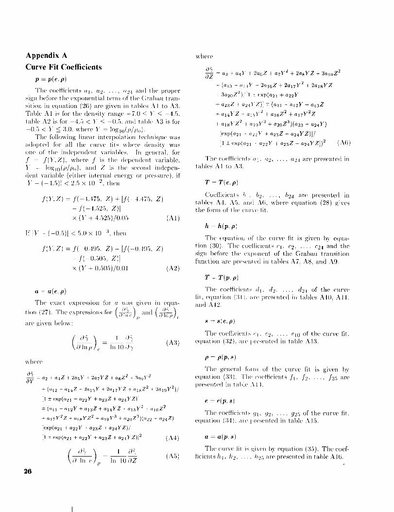
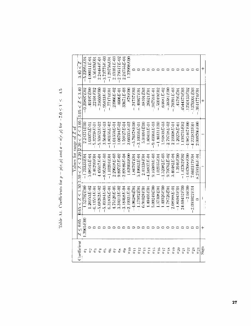
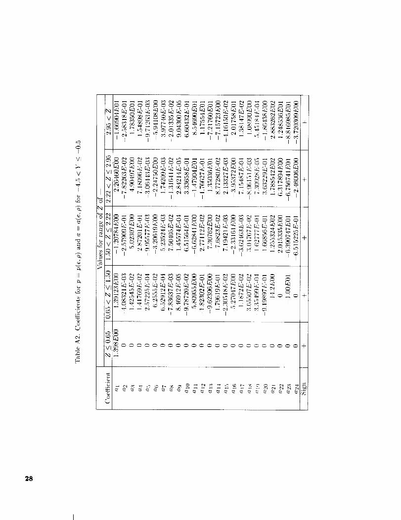
v = p)For the correlation of p = p(< p), the ratio "_ =

h/e is ClU'Ve fitted as a funclion of e and p so that pcan tie calculale(t from

p = pe(_- 1) (25)

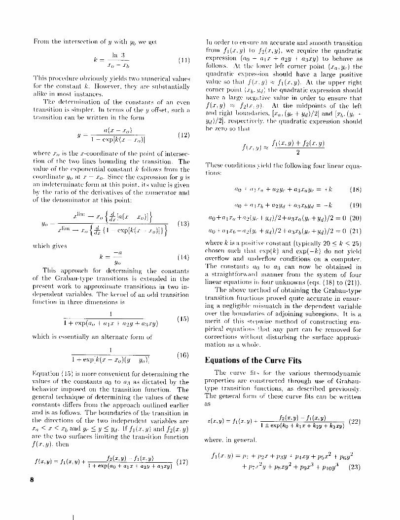
The general fornl of the equation use(t for "_ is

zt = al + a2Y + a3Z + a4YZ + a5Y 2

+ a6 Z2 + a7y2z + asYZ 2 + a9 Y3

+aloZ 3+(all +a12Y+alaZ

+al4YZ+al5 Y2 +al6Z 2 +al7y2z

+ al8YZ 2 + a19 Y3 +a2oZ3)/[1 ±exp(a21

+ a22Y + a23Z + a24Yg)] (26)

where )" = lOglO(p/po ) an(t Z = loglo(e/RTo ). Theunits for p are kg/m 3 and the units for e are nl2/s 2.

It should be noted that not all the terms appearing in

the above equation are used over the conlplete range

of e and p.

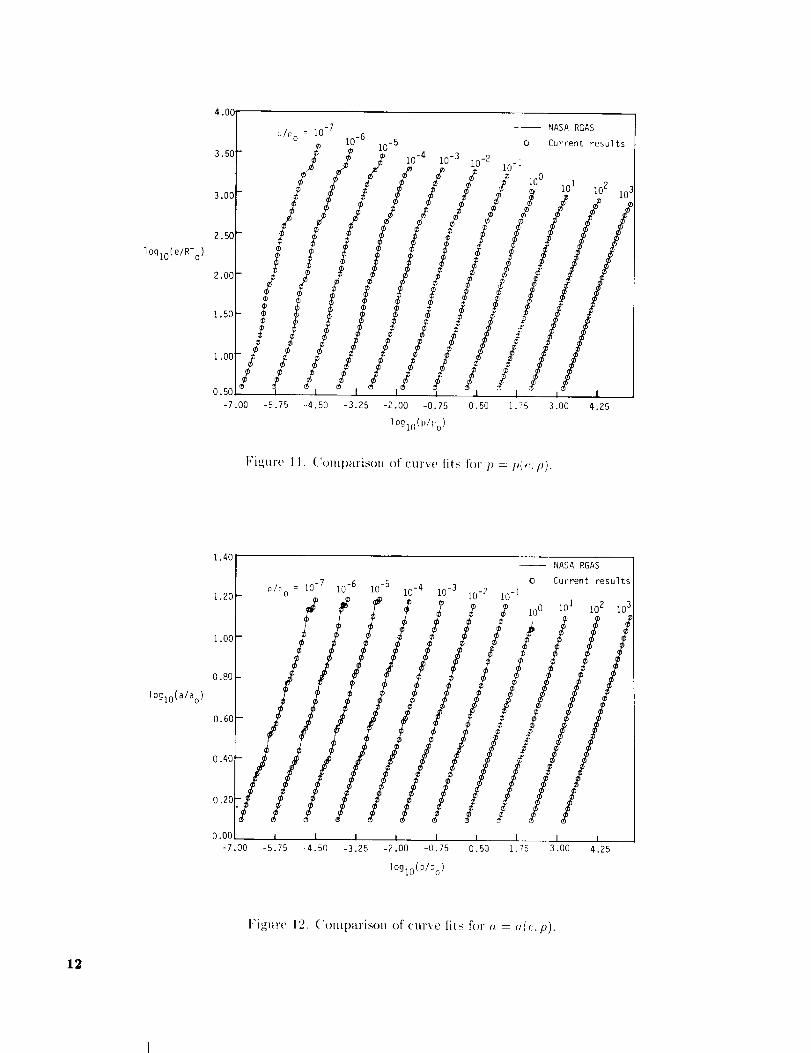
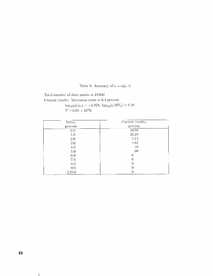
a = a(e, p)

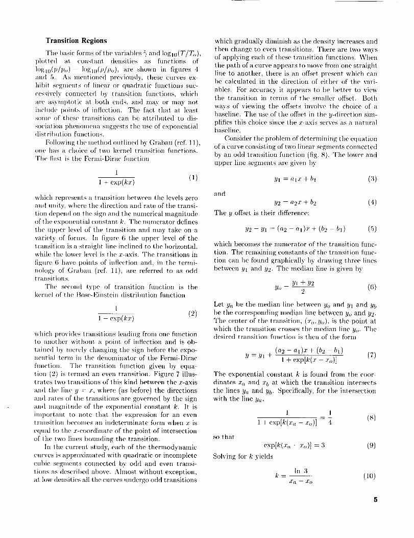
An exact, expression for the speed of sound a interms of zl was derived by Barnwell (ref. 13) and maybe written as

O_/ 05 1/2

(27)Since complete bicubic polynomials are used for

fl(Y,Z) and f2(Y,Z)- fl(I',Z)in equation (26)

for _', equation (27) is used directly for the corre-

lation a = a(e,p) without fimher corrections, un-

like in references 10 and 15. The expressions for[ ii< \ I,,',\0"t,<_ne)p and _,"_np)e are presented it, appendix A.

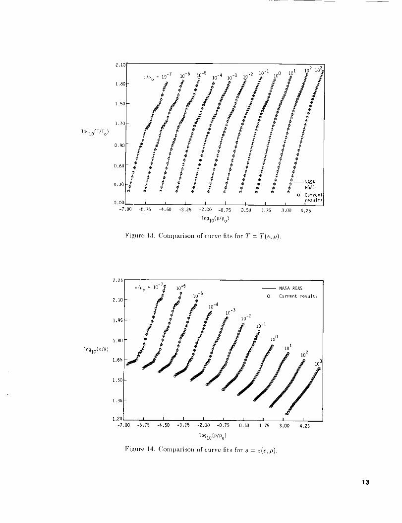
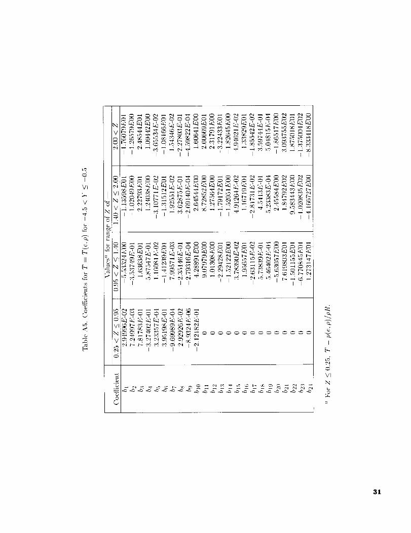
T = T(e,p)In the calculatioli of T = T(e,p), the pressure

is first, determined with equation (25), and then the

temperature is calculated with the equation

logm(T/To) = bl + b2Y + baZ + b4YZ + b5Y2 + b6Z2

+ b7Y2Z + bsYZ 2 + b9Y a + bloZ a

+(bll + bl2Y + b13Z + b14Y Z

+ b15Y _ + 516Z 2 + b17y2z + blsYZ 2

+ blgY 3 + baoZ3)/[1 + exp(b21

+ b22Y + b23Z + bi4YZ)] (28)

where Y = iogm(p/po ), X = logjo(p/po), and Z =X- Y. The units for p are N/m z, and the units for

9

T are K. The coefficients tq to b2 _ are determined iu

such a way as to eompensat(' for the errors incurre<l in

the inhial calculation of |)l'ossiil'(' \villi equation (25).

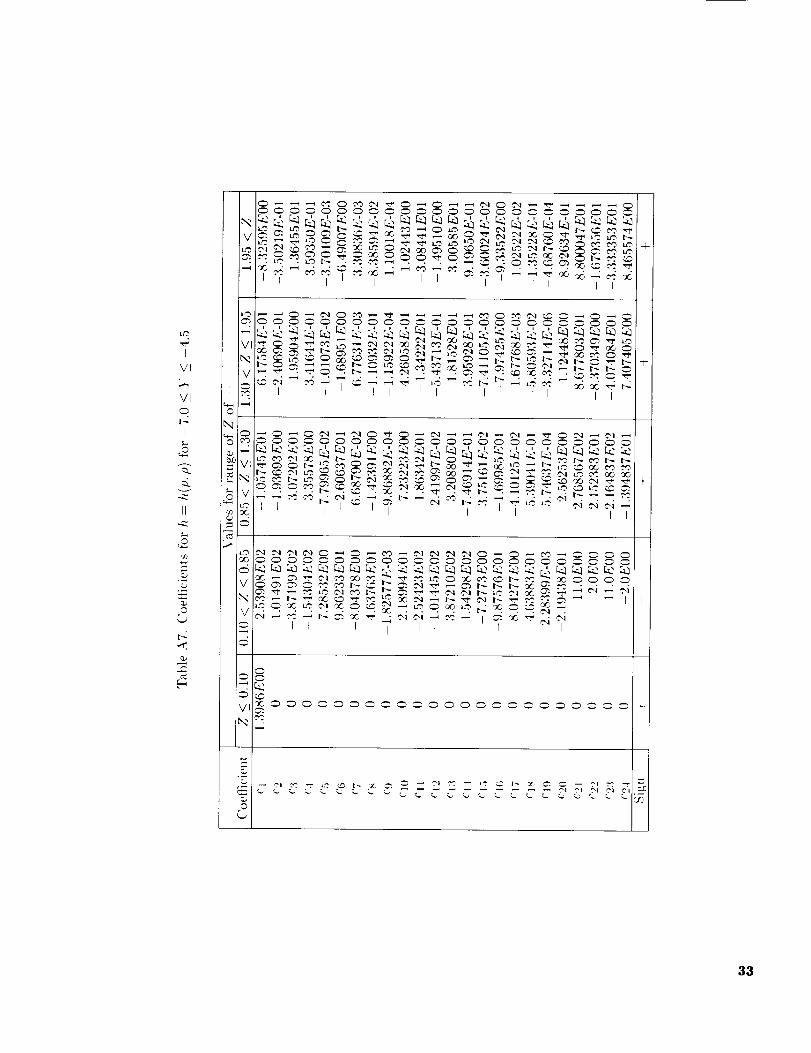
h = h(V,p)

For the correlation of h = h(l_.p), the ralio

= b/c is curve iilted as a fun('ti(m ()f" t) and p so1hat h can be calculated from

t,--(t_/t,)[¢/(_ l)l (2.())

Th(' general form of the equation used for "_,is

Cl 4- c2Y + c3Z + c4YZ _-csY 2

+ cBZ 2 + cTy2Z + csYZ 2

+ c9 Y3 + el0 Z3 + (ell 4 Cl2Y

+ c13Z+ cl4YZ + c15 Y2 _ ClBZ 2

_.c cl7y2z + clsYZ 2 + c19 Y3

+ c20Z3)/[1 ± exp(c2t ÷ c22Y

+ c23 Z + c24YZ) l (a0)

where )" = logm(p/p. ). X : lo_j0(p//_.), and Z :

.\ - _. For the correlations p = p(<,p) and h =k(p. p). where _ is the vm'iat)h, cur\(' fitted, an eventransition [unction is used to model the transition

t)(,tween th(' perfect-gas equation and the remain-

der of the curve ti't in the low(,s! (hqlsity region

(-7.0 < h)gm(p/p. ) <_ 4.50). This yields a more

accurate tit than an ordinary 1)icubi(' curve without

any t ransith)ns.

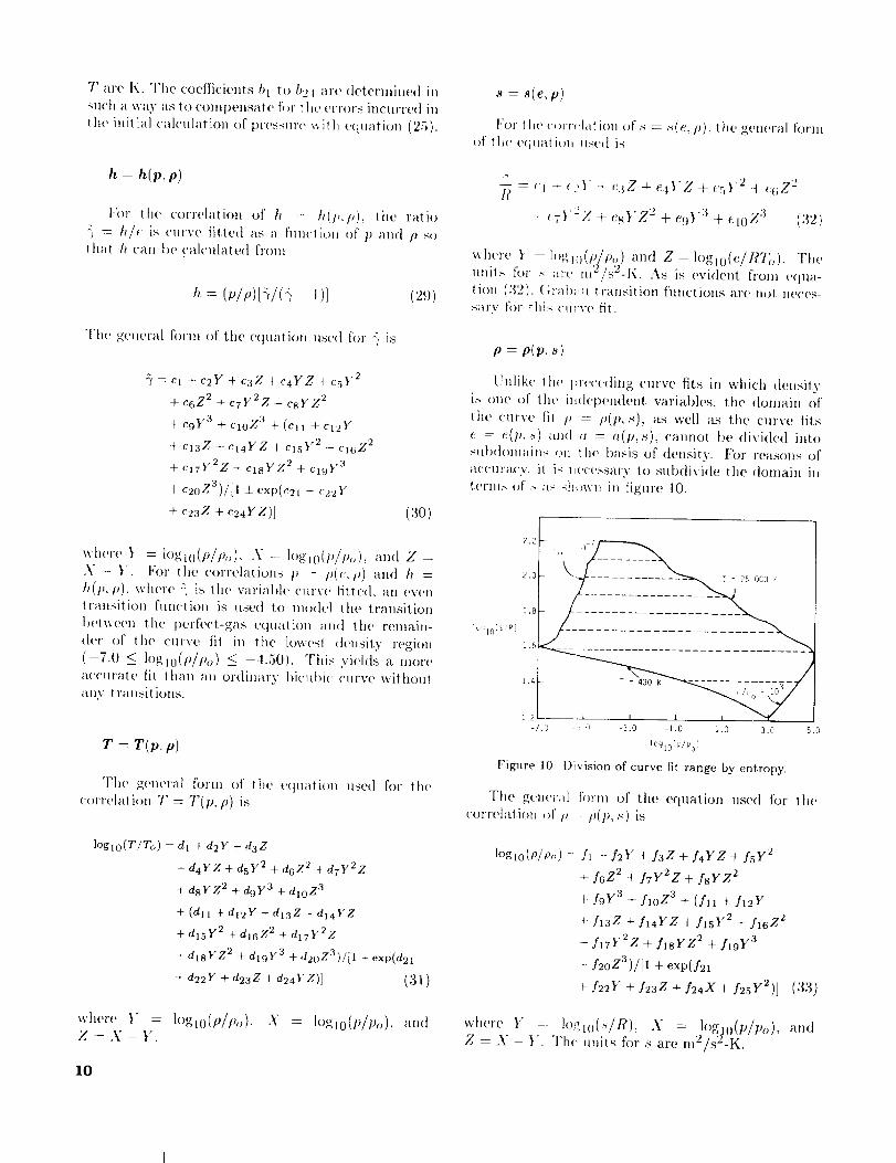
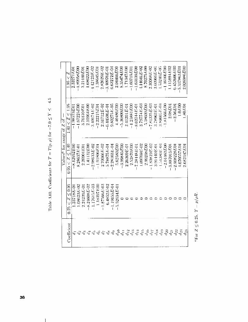
T = T(p, p)

The general fl)rm of the equation used for thr

correlation 7'-- T(p, p) is

loglO(T/To ) = d 1 + d2Y + d3Z

+ d4YZ + d5 Y2 + d6 Z2 + dTy2z

+ dsYZ 2 + d9Y 3 + dlo Z3

+ (dll + dl2Y + dl3Z + dl4YZ

+ d15 Y2 +d16 Z2 + dl7y2z

+ dl8YZ 2 + d19 Y3 +d20Z3)/[1 + exp(d21

+d22Y +d23Z +d24YZ)] (31)

where Y = logm(p/po ), X : logm(p/p,,), andZ = X - _,+.

10

s = s(e, p)

For the c,)vv_'lation of s = ,s(e, p)_ the g('n(,ral formof the equation Itsc(t is

-- -- +1 } <">_' + c?,Z + e.I}'Z + es} "2 + e.(iZ 2R

+ +:7_'2Z + es}'Z 2 + eq} <' + eloZ:" (32)

where _ _ ,/ ,) . . .h>_()(/_ p,,) and Z = log o(e/RTo). Th(,

units tc)r ,', arc ttt-/s--K. As IS evtdettt fl'om equa-tion (32). (_rat).+t transition functions are not n(,('('s-

sary for this cur\(_ til.

p = p(p,s)

Unlike lhe 1)r(,(:e+ting cm've fits in which density

is one of Ih(, independent variables, the domain of

the curve tit p _- p(p,,s), as well as the curve fits

e = e(p,.s) and a - +_(p,,+), cannot be <livi<ted into

sul)(h)mains on the basis of density. For reasons ofac('ttracy, il i_ tw(('ssary to sttbdivi(te the (tontain in

terms t>[' .* ;> _h(>wn in figure 10.

1.6

1.2

-7 .O % .O -3.0 -i .0 _.._3 3 .O 5 .O

1o910(P/%)

Figure 10. Division of curve fit range by entropy.

The gen(,ral t'<wm of the eqttation used for the

correlation of p - t'(P, ") is

lOglo(P/P,,) := ft -r- f2Y + I3Z + f4YZ + fsY 2

f6Z 2 + f7y2z 4- fsYZ 2

+ .fgY a + fmZ a + (fll +.f12Y

._ f13 Z + fl4YZ + f15 Y2 + f16 Z2

f17y2Z + flsYZ 2 +/19 Y3

-'" f2oZ3)/[1 + exp(/21

+ f22Y + f23Z 4- f24X + f25Y2)] (a3)

where 1_ -lo_.)(,ffR), X = lugm(p/p,, ), andZ = X - )'7 Th(' units for ,s are nl2/s2-K.

e - e(p, s)

For th(' correlation of e:= c(p, ,_), the general form

tff tilt' curve lit equation is

loglo(e/RTo) - gl 4- g2Y 4- g3 z 4- g4 Y Z

+ g5 Y2 +g6 Z2 +g7y2z

+ g8YZ 2 + g9 Y3 + gl0 Z3

+(gll +gl2 Y +gl3Z+gl4 YZ

+ g15 Y2 + gl6Z 2 4- glTy2Z

+ glsYZ 2 + gl9Y 3 + g20Z3)/[1 + exp(g21

+ g22 Y + g23 Z 4- g24 X 4- g25Y2)] (34)

_here Y = logu){._/t?), X = logl0(p/po), andZ = X - "_.

For Ill<' correlat ion t)f (z = o(p, .s), the general fornl

of the equatitm is

loglo(a/ao ) = h 1 + h2Y + h3Z 4- h4YZ

4- h5 Y2 + h6 Z2 + h7y2z + hsYZ 2

+ h9 Y3 4- hl0 Z3 4- (All +hl2Y

+ hl3Z + hl4YZ+ h15 Y2

+ h16 Z2 4- hl7y2z + hlsYZ 2

+ h19 Y3 4- h20Z3)/[l + exp(h21

+ h22Y + h23Z 4- h24X 4- h25y2)] (35)

where _" = lo_m(,_/R). X = logm(p/po), and

Z = X Y. The units of a are m/s.

Results and Conclusions

New, siml)lifi(,d curve fits for tile thernlodynamic

])|'operti(,s of eqlfilil)rilml air were constructed withthe pr(wedures descrit)ed in the 1)reee(ling sections.

(k)ml)arisons of the curve fits p = p(e,p), a =o(c,p), T = T(c,p), ._= .s(e,p), T = T(p,p), h =

r,(v,f,), p : /v,s), ,_- ,_(v,.4, a,,d ,, = .(p,,4wilh the original NASA RGAS wogram are shown

in figures 11 to 19. The following procedure was

(,ml)loyed in making Ill(' conq)arisons for the first four

curve fits. First, p and p data were supplied as input

t() th(' NASA R(IAS ])rograIll and e was computed.

Then, this _ and tilt' original p were used to ot)tain

p, u. 7", and ._ from tim above cm've fits. As a result

of this l)roce(lure, loglo(p/po ) is plotted as one of

the in(lepen(h,nt variables in figures 11 to 14, The

same p and p data used above were also employed in

the COUll)arisous for the cllrve fits T = T(p,p) and

h = h (/', P).The met hod adopted fi>r the COulparisons of p =

p(p,._), e = e(p,.Q, and a = a(p,._) with the NASA

RGAS t)rogram was quite sinlilar to that for the firstfour curve fits. First, p and p wet'(' supplied to the

NASA RGAS progranl, which yielded ,s. This s and

the original p were used in the above curve fits to

obtain p, c, and a.

Tile at)eve comparisons are l)resente(l grat)hically

to provide a qualitative overview of the accuracy of

the curve fits. ttowever, as figures l l to 19 indi-

cate, these graphical comparisons are rest.rieted to

points lying on 1 1 constant-density lines ranging from10 7 to 103 amagats. Ill or(let to ensure the validity

and accuracy of tim curve fits across the entire do-main, a more COml)rehensive accuracy test was car-

ried out. Tile new curve fits were compared with

the NASA R(;AS program for relative accuracies at

approximately 22 000 (tara points. These lest points

were chosen to st)an tile entire density range fromI0- 7 to 103 amagats and t emperat ures varying front

273 K to 25000 K. The results of these comprehell-

save aCcllra(:y checks are l)resente(t in tat)los 1 to 9.

For the curve fits p = p(e,p), a = a(e,p), T =

T(e,p), T = T(p,p), an(t h = h(p,p), comparisons

with the curve fits of reference 15 are also presented

in the tables. The first column in the tal)les rep-

resents the percentage error in the comparison of

a i)roI)erty generated [)y the R(;AS program and a

curve fit. The other cohmlllS contain the percent-

age of points in the l(.st tiara base, generated t)y a

curve fit, which are in error by an amount greaterthan lhat indicated in cohmnl I. The accuracies of

the present curve fits are substantially improved over

the accuracies of the previous cm've fits appearing in

reference 15. The somewhat higher t)ercentage er-

rors in the cm've fits with p and s as independentvariables can 1)e attribute(t to the fitct that a line of

constant .s spans the entire density range, sometimes

necessitating tile use of two (_t'at)au-tyt)e transition

functions. Requiring a minimal mismatch across the

junctions of these transition functions resulted in a

relative loss of accuracy. However, these latter curve

fits are well within the accuracy limits required for

most engineering af)plications.

One of the primary objectives of this research

was to minimize the discontinuities in the del)en-

dent variat)les across juncture points of tile curve fits(fig. 20). Comparisons of the (lepen(tent variables at

jllllct, llre points of the Cllrve fits for p = p(e, p), a =

a(e,p), T = T(e,p), T = T(p,p), and h = h(p,/_)

arc presented in tables 10 to 1,1. These new curve

(its showed a substantial improvement in contiml-

ity at the juncture points when COnll)ared with

the previous curve fits. For lhe cm've fits where

p and s were the independent variables, it was

very difficult to maintain continuity at the junc-

ture points. This was due to the mamwr in which

11

log10(e/RT o)

4.00

_] / i:O

3.50

3.00

2.50

2.00

1.50

i .OOt/

0.50 i

-7.00 -5.75

= 10 -7

10_6 10-5

-4.50

o

10-4 10-3 10-2 10-I

/I I I

-3.25 -2.00 -0.75 0.50 1.75 3.00

--- NASA RGAS

Current results

i01 102 103

I4.25

loglO(P/P o)

Figm'e 1I. (!onq)arisoH of curve fits Cot p : p(_. p).

loglo(a/a o)

1"40 I

i .20

i .00

0.80

0.60

0.40

0.2C

0.00

-7.0

p/r, ° = 10 -7 10-6

I I I

-5.75 -4.50

10-5 10-4 10-3 10-2

l

I I I-3.25 -2.00 -0.75 0.50

loglO(P/P o)

.... NASA RGAS

0 Current results

10-1

100 i01 102 103

/I I I

1.75 3.00 4.25

Figure 12. ('onq)arison of curve fits for. = .(e,p).

12

2.10

I. 80

p/% = 10-7 10-6 10-5 10-4 10 -3 10 -2 10 -I i00101 102 10 j

1.50

i .20

IOglo(T/T o)

0.90

0.60

0.30

0.00 I I I I I I I I

-7.00 -5.75 -4.50 -3.25 -2.00 -0.75 0.50 1.75 3.00 4.25

lOglo(P/P o)

Figure 13. Comparison of curve fits for T = T(e, p).

IoglO(S/R)

2.25

2.10

1.95

i .80

i .65

1.50

1.35

_IPo = 10-7m_ 10-6

10 -5

i0_4

10-3

1.20 1 I I I I

-7.00 -5.75 -4.50 -3.25 -2.00 -0.75

-- NASA RGAS

Current results

10 -2

i0 -I

10 0

101

l0 2

I I I I

0.50 1.75 3.00 4.25

IOgIo(P/P o)

Figm'e 14. Comparison of curve fits for _ = 3(e, p).

13

loglO(T/T o)

2.10

1.80

1.50

1.20

0.90

0.60

0.30

_i0 -7 10-6 a- 5 I0-4 10-3 i0_2 !-i

o///

t

o .o0 i I I I I I I-7.00 -5.75 -4.50 -3.25 -2.00 -0.75 0.50

100 101 i0

--NASA

RGAS

o Currentresults

L ..... I I

1.75 3.00 4.25

loglO(P/P o)

Figure t 5. Comparison of cm'vc fits for 7" = 7"(p. p).

loglO(h/RT o)

4°° l 10_7 10-6-- NAS# RGAS

3.50

3.00

2.50

2.00

1.5C

1.00

c/c 0 =

/I I I

10 -5 10_4

I

10-3 10-2 10-i

0.50-7.00 -5.75 -4.50 -3.25 -2.00 -0.75 -0.50

0 Current results

I00 i01

i i I i I1,75 3.00 4.25

IOglo(P/P o)

Figure 16. Comparison of curve fits fol" h = h(p, p).

14

IoglO(P/%)

2.50

i .00

-0.50

-2.00

-3.50

-5.00

-6.50

-8.00-7.00

mme_em_e_em_mm

-- NASA RGAS

o Current results

I I I I I I I I I3.00 4.25-5.75 -4.50 -3.25 -2.00 -0.75 0.50 1.75

IOglo(P/P o)

Figm'e 17. Comparison of curve fits for p = p(p, ,_).

Ioglo(e/RT o)

4.oo I

3.50

3.00

2.50

2.00

I. 50

1.00

O. 50-7,00

log10(P/P o)

Figure 18. Comparison of curve fits for e = e(p, ,s).

-- NASA RGAS

Current results

I01

I- I3.00 4.25

15

loglo(a/a o)

i .40

1.20

i .00

0.80

0.60

0.40

0.20

0.00 I-7.0

-- NASA RGAS

C/_o = 10-7 10-6 10-5 10-4 10-3 10_ 2 10_i 0 Current results

- 10 0 10

/ /I I I I I 1 I I

-5.75 -4.50 -3.25 -2.00 -0.75 0.50 1.75 3.00 4.25

IOglo(P/P o)

Figure 19. Comparison of curve fits for (1 = _(p, ._).

16

very difficult to maintain continuity at the junc-

ture points. This was due t.o the manner in which

the domain was subdivided to obtain the piecewise

approxinlating functions. However, discontinuities

were kept to a minimum, with average mismatches

of 2.4 percent for p = p(p,s), 1.2 percent for a =

(l(p, ,_), a,ld 2.0 percent for e = e(p, ,s).

3.90

_'IPo : 10-7

3.40 _u rye/_

2.40 C #Curve 4 /

lo910(e/RTo ) }( / Grabau.- type

1.40 Cur

o./V/-7.00 -6.50 -6.00 -5.50 -5.00 -4.50 -4.00

log10(P/P o)

Figure 20. Example curve fit for p = p(e, p).

A conlparison of the relative computer times re-

quired for the new curve fit subroutines and the

NASA RGAS program on the National Advanced

Systems 9160 computer is given in table 15. The

new subroutine for determining p = p(e,p), a =

a(e,p), and T = T(e,p) was 2.4 times faster thanthe NASA RGAS subroutine. The previous subrou-

tine (ref. 15) for the same curve fits was 3.4 timesfaster than the NASA RGAS subroutine. The new

subroutine for T = T(p,p) was 2.7 times fasterthan the NASA RGAS subroutine, and the previ-

ous subroutine (ref. 15) was 3.4 times faster. The

new subroutine for h = h(p, p) was 3.2 times faster

than the NASA RGAS subroutine, compared with

the previous subroutine (ref. 15), which was 4.4 times

faster. The subroutine for ,s = ,s(e, p) was 10.2 timesfaster than the NASA RGAS program. The new

subroutines for the curve fits p = p(p,s), e =

e(p, s), and a = a(p,,s) were approximately 10 timesfaster than the NASA RGAS subroutine. It should

be noted that the NASA RGAS program requires two

data files for storage of the cubic interpolation coeffi-cients. The fact that these data files are now on disk

and not tape has significantly speeded up the NASA

RGAS subroutine. However, the curve fits still pro-

vide a substantial improvement in computing time,

being 2.4 to 10.2 times faster than the t.able-lookup

technique.

In conclusion, the new, simplified curve fits for the

thermodynamic properties of equilibrium air provide

substantial reductions in computer time and storage

while maintaining good accuracy. They can be in-

corporated into computational fluid dynamics com-

puter codes in a straightforward manner without theneed for data files. The improved accuracy of the

new curve fits permits their use in time-dependent

flow calculations from start-up to the final steady-

state solution. In addition, the improved continuity

of these curve fits permits their use in iterative calcu-

lations. For example, the new curve fit. for h = h(p, p)

can be employed in the iterative procedure requiredto "fit" a bow shock in equilibrium flow. However,

the discontinuities which still exist in the entropy

curve fits may cause difficulties when used in an it-erative shock calculation.

NASA Langley Research CenterHampton,Virginia 23665-5225

May 1, 1987

17

Table1. Accuracyof p = p(_./,)

Tot al number of data points -- 22 239

('urreut results: Maximum error= 3.93 percent

loglo(p/po) = 4.0; lOglO(e/t?7;, ) = 3.28

7"= 1.47 × 104K

Ref. 15 results: Maximum error = 9.00 percent

loglo(p/po) .... 4.5 loglo(e/RT,, ) = 2.23(5

7" = 4.53 × 103K

Error, Current resulls. Results fl'om

percent percent ref. 15, percent0.5

1.0

2.03.0

,I.0

5.0

6.07.0

8.0

9.0>10.0

28.43

10.63

1.01

.03

00

0

0

0

0

0

68.29

,12.87

17.51

6.691.4!)

.24

.14

.04

.01

0

0

Table 2. Accuracy of _ (1(_. p)

Total tmmt)er of data points = 22 239

('re'rent results: Nla-<imum error = 4.,18 percent

loglo(p/po) =-3.0; loglo(e/t_To) = 3.31_

7' = 2.0 × 104K

Ref. 15 results: Maximum error = 4.94 percent

loglo(p/po) ==-7.0 log,0(e/RTo ) 3.279

T = 1.25 × 104K

Error, Current results, Results fl'om

percent percent ref. 15, percent0.5

1.02.0

3.0

4.0

5.0

6.0

7.0

8.0

9.0

>10.0

20.94

5.75

.70

.09

.020

0

0

0

0

0

60.67

27.215.17

.98

.11

0

0

0

0

00

18

Table3. Accuracyof T = T(e, p)

Total mmlber of data points = 22 239

Current results: Maximum error = 4.36 percent

l,,gm(p/p,) ---4.0; logm(e/_Z,) = 3.2s7'= 1.47 × 104K

]{ef. 15 results: Maximum error = 8.8 percent

loglo(p/p,,) = -0.(32,5; lOgl0(e/RTo) = 3.255

7"= 2.4 × 101K

Error, Current results, Results from

per(:ent, percent ref. 15, percent0.51.0

2.0

3.0

i.O

5.0

6.0

7.0

8.0

9.0

> 10.0

;{4.11

10.87

.58

.10

.01

0

0

0

0

0

0

63.82

34.74

9.51

2.4;{

.59

.19

.09

.04

.02

00

Table 4. Accuracy of s = s(e, p)

Total numt)er of (lata points = 21 975

Current results: Maximum error = 2.51 percent

loglo(p/p¢_) = -0.625; logm(e/RT,, ) = 0.657

T = ,1.89 × 102K

Error, Current results,

percent percent0.5

1.0

2.0

3.O

4.0

5.06.0

7.0

8.0

9.0

10.0

49.77

15.95

.56

0

0

00

0

0

0

0

10

Table,5.Accuracyof T = T(p, p)

Total nuiiit)er of (tala points = 22 239

Current results: Maxinmm error = 3.9 percent

logm(p/p,,) -- -3.25 logm(p/po ) logm(l_/p,, ) = 2.58

T = 2.4 x 104K

Ref. 15 results: Max,reran error = 5.71 t)ercent

log m (/)/P,,) -- -0.625; log m (p/po) - log ill(/'�P(,) = 2.44

7' = 2.3 × 104K

Error, Current results, Results from

percent percent ref. 1.5, percent0.5

1.0

2.0

3.0

4.05.0

6.0

7.0

8.0

9.0

_>10.0

22.89

8.24

.22

.03

0

0

0

0

00

0

58.82

28.75

4.89

.96

.16

.04

0

00

0

0

Table 6. Accuracy of h = h(p, p)

Total number of (tara points = 22239

('UFl'ellt results: Maximum error = 3.44 percent

loglo(p/p<,) := -7.0; logio(p/po ) -lOglo(P/p,, ) = 2.60

T= 1.91 × 10'IK

Ref. 15 resuhs: Maxiimmi error = 6.56 percent

hJgio(p/p,) .... t.5; lOglo(p/po ) -logl0(;,/po ) = 1.01

T = 2.47 × 103K

Error, Current results, Results from

percent percent ref. 15, percent

0.51.0

2.0

3.0

4.0

5.0

(i.O

7.0

8.0

9.0

__10.0

23.85

7.65

.55

.04

0

0

00

0

0

0

67.45

40.36

13.65

4.78

1.56

.46

.16

0

0

0

0

2O

Table7. Accuracyof p = p(p, s)

Total mnnber of data points = 21 030

Current results: Maximtun error = 7.58 percent

logl0(p/po) = -6.625; loglo(e/RT,, ) = 3.30

T = 1.42 x 104K

Error, Current results,

percent percent0.5

1.0

2.0

3.04.0

5.0

6.0

7.0

8.0

9.0

10.0

62.06

40.25

14.97

4.46

.98

.35.03

.01

0

00

Table 8. Accm'acy of e = e(p, s)

Total number of data points = 21 030

Current results: Maximunl error = 4.5 percent

logm(p/po) = 2.875; ]ogm(e/RTo ) = 2.85

T = 2.46 x lO'lK

Error, Current results,

percent percent0.5

1.0

2.0

3.0

4.0

5.0

6.0

7.0

8.0

9.0

10.0

39.52

22.68

5.45

.04

.01

0

0

0

0

0

0

21

Ghble9. Accuracyof a = a(p_,_)

Total umnber of data l>Oint.s = 21 030

Current, results: Maximum error = 6.1 percent

log _o (tUt_-) -- -- 2.375; log_o (c/177<,) = '2.3!)

7' - 6.05 × 103K

Error, Curront results,

porcent t)erccnt0.5

1.0

2.0

3.0

<1.0

5.06.0

7.0

8.0

9.0

> 10.0

5().9S

26.2S

5.71

1 ,(i7

,(iS

_)0

0

0

0

22

Table 10. Comparison of Variables at Juncture Points for p = p(e, p}

Density

ratio,

p/po

10 ,7 1.79 × 10 2

10 6 1.79 × 10 1

10 5 1.79 x 10 °

l0 4 1.80 _ 101

111 3 1.80 × 102

10 -2 1.8/I _ 103

10 1 1.80 _ 104

100 1.80 × 105

101 [.80 × 106

102 1.80 _ 107

103 1.811 x 1118

Point A* Point B* Point C* Point D*

I,ower Upper Lower Upper Lower Upper Lower Upper

1.81 × 10 2

1,80 × 10-1

1.80 × 100

1.81 "_ 101

1.81 × 102

1.81 × 103

1,81 _ 104

1.81 × 105

1.81 × 106

1.81 × 11) 7

1.83 × 108

7.32 × 10 -2

7.81 × 10 I

8.17 × 100

8.67 × 10 I

9.12 × 102

9.51 × 103

9.80 ,_ 104

1.36 × 106

1.41 × 107

1.45 × 108

1.48 × 109

7.,38 × 10 2

7.78 × 10 1

8.19 × 100

8.70 × 101

9.13 × 102

9.,51 × 103

9.81 × 104

1.36 × 106

1.41 × 107

1.43 x 108

1.45 × 109

1.90 × 10 -1

2.01 × 100

2,16 × 10 l

2.40 x 102

2.61 × 103

2.83 × 104

3.08 × 105

4.11 x 106

4.50 × 107

4.91 x 108

5.42 x 109

1.911 × 10-1

2.03 × 100

2.18 × 101

2.43 x 102

2.63 × 103

2.84 x 104

3.08 × 105

4.11 × 106

4.54 × 107

5.00 × 108

5.53 x 109

8.72 :,: 10 1

9.53 × 100

1.05 × 102

9.78 × 102

1.09 x 104

1.23 × 105

1.39 × 106

8.72 × 10-I

9.63 × I00

1.06 × 102

9.79 × 102

1.09 × 104

1.23 × 105

1.39 × 106

*See figure 20 fi)r curve breaks.

Point E*

Lower Upper

2.62 × 100 2.63 × 100

2.86 × 101 2.89 × 101

3.15 × 102 3.16 × 102

1.80 × 102 1.81 × 102

Table 11. Comparison of Variables at Juncture Points for a = a(e, p)

Density

ratio,

p/po

10 -7

10 -6

10 5

10 -4

10 -3

10 2

10 -1

100

101

102

103

Point A* Point B* Point C* Point D* Point E*

Lower U pper Lower U pper Lower UpperLower Upper

440 441

440 439

,t40 438

441 440

441 440

441 440

441 441

442 441

442 440

442 440

442 441

Lower U'pper

769 790

808 814

831 841

869 874

902 904

932 932

957 957

1120 1118

1149 1145

1171 1164

1188 1179

1250

1291

1343

1429

1498

1573

1655

1924

2027

2141

2287

1260

1307

1359

1441

1506

1578

1656

1924

2039

2166

2312

2718

2857

3021

2923

3115

3337

3596

2733

2871

3029

2925

3116

3341

3602

4731

4983

5259

4715

5016

5287

*See figure 20 for curve breaks.

23

Table 12. Comparison of Variables at Juncture Points for T -: T(e,p)

Density Point A*

ratio,

p/po Lower Upper

10 -7 486 481

10 -6 486 482

10 -5 486 484

10 -4 486 481

10 3 486 481

10 2 486 481

10 -1 486 481

10 ° 486 482

101 486 482

102 486 482

103 486 483

Point B*

Lower

2112

2181

2243

2312

2347

2376

2400

2408

2413

2416

2418

Point C*

Upper Lower

2091 4033

2168 4283

2243 4548

2312 4837

2366 5090

2404 5307

2417 5508

2414 6242

2416 6585

2416 6955

2419 7317

Upper

4034

4284

4548

4818

5088

5326

5517

6265

6595

6960

7328

mlt D* Point E*

Low, Upper

78(

84q

914

10 3(

11 1(.

11 9,"

127

Upper Lower

7 869

8 479

9 146

10 319

11 177

12 006

12 738

*See figure 20 for curve breaks.

Table 13. Comparison of Variables at Juncture Points for T := T(p, p)

Density Point A*

ratio,

P/Po Lower Upper

10 -7 486 482

10 6 486 482

10 -5 486 484

10 4 486 482

10 3 486 481

10 -2 486 481

10 1 486 482

10 ° 486 482

101 486 482

102 486 483

103 486 483

Point B*

Lower Upper

2089 2089

2165 2165

2242 2242

2310 2310

! 2363 2363

2404 2404

2402 2402

2706 2700

2706 2710

2711 2712

2713 2713

Point C*

Lower

4025 4033

4281 4281

4549 4554

5064 i 5042

5386 5376

5690 5701

5968 5998

6248 6267

6585 6598

6950 6959

7309 7319

Upper Lower

7864

8470

9,1t6

10 796

1 7921

i 12 742

13671

,int D*

Upper

I 7838

8481

! 9146

10 746

11682

12 679

13 687

Point E*

Lower Upper

*See figure 20 for curve breaks.

24

Density

ratio,

p/Po Lower

10 -7 0.346 × 106

10 6 .346

10 -5 .346

10 4 .346

10 3 .346

10 2 .346

10 -I .346

10 ° .345

101 .345

102 .345

103 .345

Table 14. Comparison of Variables at Juncture Points for h = h(p, p)

Point A* Point B* Point C* Point D*

Upper Lower Upper Lower Upper

0.346 × 106 0.282 × 107 0.285 × 107 0.160× l0 s 0.159 × 108

.346 .253 .254 .138 .138

.346 .233 .235 .120 .122

.346 .345 .345 .247 .247

.346 .314 .315 .214 .214

.346 .296 .296 .186 .186

.346 .288 .288 .164 .164

.345 .386 .387 .201 .202

.345 .377 .380 .180 .181

.345 .374 .376 .166 .166

.345 .374 .374 .156 .156

Lower Upper

0.997 × 108 0.997 × 10 s

.890 ,890

.793 .792

.812 .813

.720 .721

.646 .646

.590 .591

Point E*

Lower Upper

*See figure 20 for curve breaks.

Table 15. Comparison of Computer Times

Curve fit

l, : r,(_, p)a = .(,_, p)T : v(_, p)._= ._(e,p)V = V(p, p)h = h(p, p)p =/p, ,_)e = e(p, ,_). = .(p, ._)

Nunlber of

data points

10661

10661

9921

9921

3 038

3 038

3 038

Colnputer tilne, s, for

Oldsubroutine

(ref. 15)

0.54

.25

.19

Ncw

subroutine

0.77

.20

.31

.26

.lO

.ll

.ll

NASA RGAS

1.86

2.03

.84

.84

1.07

1.06

1.06

25

Appendix A

Curve Fit Coefficients

p p(e,p)

"I'll(, coetticielllS "1, a2 .... , a2. I _lll(t the proper

Si_ll hcf'ore the exponential tel'Ill ()[ thc (;I'.:lt)_tll trail-

sition in equation (26) are given in tal)les A1 to A3.

Table A1 is for the density l';-illge -7.0 <__ }" _ --/t,5,

lable A2is for 4.5 < )" < -0.5, and table A3 is for

-0.5 < }" _< 3.0. where t" = loglo(P/p,, ).

The following linear interpolation technique was

adopted for all fhe curve fits where density was

one o[ flit' ill(tependt,nt varial)h,s. In general, for

f = .f(_,',Z), where f is the dependent variable,

}" = Iogl0(p/po ), and Z is the second indepen-

dent variabl(, (either internal energy or pressure), if

I}" - (-.1.5){ < 2.5 x 10 -2, then

f(}, Z) = f(-.1.475, Z) + [f(-.t.,t75, Z)

- f(-4.525, Z)]

x (_+ 4.s2s)10.0s (A l)

If It-" - (-0.5)l < 5.1) x It) a, then

f(}.Z) = f( 0.,t95, Z)÷[f(--O..195, Z)

- f(-0.505, Z)]

x (_ + 0.s0.S)lo.0J (A2)

a : ate, p)

The exact expression for (_ was given in equa-

lion (27). The expressions for (_ and [_i) In _' ] p /\OInp ,

are given below:

Ohlp/_, lnl()_(Aa)

V,dlel'e

O_ _ ,,-- = a 2 + a4Z + 2a5Y + 2a7YZ + a8 Z2 + : a 9}oY

+ (a12 +a14Z+2alsY +2al7YZ+alsZ 2 ÷°,al9y2)/

[1 ± exp(a21 + a22Y + a23Z + a24}"Z)]

7: (al 1 + al2Y + al3Z + al4YZ + a15 Y2 + a16 Z2

+ al7y2z + a18YZ 2 + al9Y 3 + a20Z3)(a22 + a24Z)

[exp(a21 + a22Y + a23Z + a24YZ)/

[1 ± exp(a21 + a22Y + a23Z + a24YZ)} 2 (A,i)

(0.,) _ 1 ,,% (AS)iJ hi e v hi 100Z

26

whel'("

a_OZ

-- a3 -7 a4}" + 2a6Z + a7 Y2 -- 2asYZ + 3aloZ 2

÷ (a13 + allY" -- 2a16Z+2a17Y 2 +2al8YZ

+ 3a20Z'2)/[1 i: exp(a21 + a22Y

+ a'eaZ + a'._,4YZ)] :7 (all + a12Y + alaZ

+ al4YZ + a15 Y2 + alfZ 2 + alrY2Z

a1811,'/2 ,L al!)y 3 + a20za)(a23 + a24Y)

[exp(a21 " a22 }_ f a23Z + a24YZ)]/

[1 -kexp(a21 + a22Y + a23Z +a24YZ]) 2 (A6 )

The coeflit'ienls "l. w2, ..., o2.1 are presented in

tabh,s A1 to A3,

T= T(e,p)

Coefticiems t_l, b2, ..., b24 are presented in

t al)les A.1, AS, anti A(i, where eqltation (28) gives

the fornl of the (':lrv(' fit.

h = h(p, p)

Th(, (,qlmli()n of the curve fit is give]l by equa-

tion (30). The coelticients el, c2 .... , c24 and the

sign i)efore th(' e-q)(ment of tim Grabau transition

func'lion g.tF(' l)res(,nlt,d in tal)les AT, A8, and A9.

T : T(p, p)

The coefliciems d I . d2, ..., d2.1 of the curve

tit, ('qllat i(.ql (31). ;tr(, presente(t in tables A10. All.

all(l A 12.

s = s(e, p)

Tile ('oeflic'ie_ltS "1, c.2 .... , CI0 of lhc CllrVe tit,

equation (32). are iwc'Selllett ill tal)le A13.

p - p(p, s)

The general I'orui of tile eurve fit, is given t)y

equation (33). The ('()('tficienls fi, f2 .... , f25 are

l)reseill('(I in faille .\ II.

e = e(p, s)

Tim coeflicienls !ll, g2 ..... g25 of tile curve fit,

equation (3.1). a re' l )r('.senle(t ill I al)le A 15.

,, = <p, *)

The curvc tit is ,,_i_('n by equation (35). Tile coef-

fici(mt.s hi, h 2 ..... ]_23 are presented in table A16.

Iv_

v_

q

_0

H

r_

d

II

©

c,

v

o

Vl

V

jL.O

v

v

I E

_ _ _ _ _ _ _ -- _ _ _ _ _ _ _ I_ _

I i'1" ": II i I I I _N_._II

÷

+

I Lo -d _ "_i I

_.._. _.

©

+

2'7

©

÷

÷

-I-

+

+

28

vl

v

I

J

H

J

N

r_

©

.<

L_

VI_N

V

b,-

v,N

V

+

_ _._ _. _ .___

I _ I I II II

+

I II

+

C_

¢,i

O!

39

I

VI

,.....

VIC;

I

E-.11

©

VI

©

V

T_C

V

q ' I I I I I ( q I

L_ _ _ •_ _ b m m .,-,i .--i_'_ z_ _._ _ L_ C'_ '_ _ _ _ _

._ . _ _ .___-:_--: .__ _ '_ _-_.I I I I / I "1" _ "l" I I

_ _-- _ I _ _ _ _ _ _ . _ _ _ _ _ _I 1 II "I" I I Iii

Vi_ _ _ _ _ ¸ _ _ _ _

_ _ _

]l I II

_L

14

VI

3O

L"_.

I

VI

v

,,dI

d

II

©

,2.;,

q,

..,C_,

I0

L_

b_

I I II I I I II

©

II

I."2.

vI_q

31

VI

V

I

II

+--

Q_

#

i

g_

VI

VL'D.

oi

_ _ _ _ _,_ _ _ _

_q_qqqqqq_

_,_ _

L_

VI

32

IVI

VI

I

II

©

_4

r r I I

vI

v

0

V_

V

O(5

_5

VI

b_

V

d

II

i I li I I II

__l _ __..... _ . _ . _

-- _ _ _ _ _ _ _ _ _ _ _ _ _ _ _ _ _ _ _ _ -- -- _I I I _ _ _ _I '

___ ___l_

___ ' "_ • •

II I I II I I I

+

÷

÷

+

©

33

V __ _¢_¢_Sk_e_zq'8_ ..... __ -

• _

I I F I]

4-

I

Vl

VLC

I

H

2

0

V

V

b_

ce-:

_ v_

.2 _v

_. -t, _ .'_. _. ''_" _'_ I_';

?i '_ _4 " _ : " " _-; "_ ,-_ -- ' .9 _'_. " -'; _ -_?

" TT i i' /

O_ O0

II I ]1 I

i)G 1"_ ._. Im-

._, _. _ _ -

I I

V _ • _-: _' " _: • . b- ............. | _ .. _ _ . _ _ 0_., ,_C, r'_l ,-_ .':'C _ --._

I I I i I I I I I -_ " _ "I I

N--:

©

0

4-

4-

4-

)C

34

IVl

v

I

q_

Cc,

.<q.*

©

+

+

+

0

35

L._

vI

Iv+VI +-+-_+

_ V

+-+

v-u

v.,...++

,- VI

-_ V

e+

,__-_ - __

-- _ _ _ _ ,___ _ _ +-_ ___" . _ ._ ._I_ .

tl I I II III _"L +

+ I I I I "l" I i l I _ + _il

--_-- __

II ItII

Vl

36

I

VI

V

I

II

©G,

.,<

L©

_qVl

V

> V

c5

_ .__ ._ __m-___ I _N__ _

I I II I Ill I_-

-_= ___ 8g_

I It I I I

II

©

VI

37

Ivb

v

o

d.

II

3'3

©

E.-

0

_v

>.

O__O___C ____ _

I I I I II

_--_ r_ _ _ ,'_ _ _"3 _ "_ _ _ .--_ _ "_ C".I _ r_ "-_ "_" "-_ _1 '--_ C"I--'_.. ,--.,

_ _ _ _ _ a:___=__

I I I I .

_ ¢_, _-.T ,--.._ ...,_ -_,._ _".q _._ _ L._. _-'_

u__ I I I I

VI

38

II

0

i

o vl

_v

I

%

V__

vem___ ..

I I

0

-___

_ _, _-_ _. _ _- _ _- _.

ao

4-

b,-

II

VI

39

B,_ i t)-__ /_'_

V

_4

V

'VI

t

I _ I_ I

I VJ AI

V _

VI

AI I

t

i

I

F Ii _'I

I !1 _

I I

_ . _ - _ ,_ ,

1

g.

v

&o

£

tl

o

VI

e_

Vi _' +0A

I _

V_ ,_ +

t_

£A,.4 N

v _

Vb _

_ I ar

_ N

m.4

V

V

Vl

Vb

n

8

/ I

_ _ _ __ _ _ _ I

4 _7I I

I

_ °_oo. __ _ _1

I

I I I

..... _ _o_o=_ °oI

I

i

• m

_7_ I _'_'1

I

+

II

#

_=

v

41

H

L_

+

t

H

%

V

_q

42

Appendix B

Master Program

All the curve fits developed in this study have

been incorporated into a single master program

called TGAS. This master l)rogram permits the userto select tile desired curve fit from a menu of pos-

sibilities. Tile calling statement for this subroutine

is

CALL TGAS (P,RHO,E,H,T,A,S,NTGAS)

where

P

RHO

E

H

T

A

S

NTGAS

pressure, N/m 2

density, kg/m a

specific internal energy, Ill2/S 2

specific enthalpy, ln2/s 2

t,emperat ure, K

speed of sound, m/s

specific entropy, m2/s2-K

integer flag to be set,

by the user for selectionof the appropriate curvefit as follows:

NTGAS = 0: p = p(e,p)

NTGAS = 1: p=p(e,p),

a = a(e, p)NTGAS = 2: p = p(e,p),

T = T(e, p)

NTGAS = 3: p = p(e,p),

_ = o(e, p),T : T(e, p)

NTGAS = 4: .q = s(e,p)NTGAS = 5: T = T(p,p)

NTGAS = 6: h = h(p,p)

NTGAS = 7: p=p(p,s)

NTGAS = 8: e= e(p:s)NTGAS = 9: a = a(p,s)

The curve fits for p = p(e, p), a = a(e, p), aim T =

T(e,p) have been placed in the single subroutineTGASI. Subroutine TGAS2 computes ,s = s(e, p), sub-

routine TGAS3 computes T = T(p,p), and subrou-

tine TGAS4 computes h = h(p,p). The curve fits for

p : p(p,s), e = e(v,,s,), and a : a(p,s) have been

placed in subroutines TGAS5, TGAS6, and TGAS7, re-spectively. The subroutines TGAS1 to TGAS7 can beused in a "stand-alone" manner if so desired, inde-

pendent of the master program. A FORTRAN listing

of each subroutine is given in reference 18.

43

References

1. Gilmore, F. R.: Equilibrium Composition and Thermody-

namic Properties of Air to 2J,O00 ° K. U.S. Air Force Proj.

Rand Res. Memo. RM-1543, Rand Corp., Aug. 24, 1955.

(Available from DTIC as AD 840 52.)

2. Hilsenrath, Joseph; and Beckett, Charles W.: Ta-

bles of Thermodynamic Properties of Argon-Free Air to

15,000°K. AEDC-TN-56-12, Arnold Engineering Devel-

opment Center, Sept. 1956. (Available from DTIC as

AD 989 74.)

3. Hansen, C. Frederick: Approximations for the Thermody-

namic and Transport Properties of High- Temperature Air.

NASA TR R-50, 1959. (Supersedes NACA TN 4150.)

4. Moeckel, W. E.; and Weston, Kenneth C.: Composition

and Thermodynamic Properties of Air in Chemical Equi-

librium. NACA TN 4265, 1958.

5. Bailey, Harry E.: Programs for Computing Equilibrium

Thermodynamic Properties of Gases. NASA TN D-3921,

1967.

6. Zeleznik, Frank J.; and Gordon, Sanford: A Gen-

eral IBM 70,_ or 7090 Computer Program for Computa-

tion of Chemical Equilibrium Compositions, Rocket Per-

formance, and Chapman-Jouguet Detonations. NASA

TN D-1454, 1962.

7. Gordon, Sanford; and McBride, Bonnie J.: Computer

Program for Calculation of Complex Chemical Equilib-

rium Compositions, Rocket Performance, Incident and

Reflected Shocks, and Chapman-Jouguet Detonations.

NASA SP-273, 1971.

8. Miner, E. W.; Anderson, E. C.; and Lewis, Clark H.:

A Computer Program for Two-Dimensional and Axisym-

metric Nonreactin9 Perfect Gas and Equilibrium Chem-

ically Reacting Laminar, Transitional and-or Turbulent

Boundary Layer Flows. VPI-E-71-8 (Contract NAS1-

9337), Dep. Aerospace Engineering, Virginia Polytech-

nic Inst., Jan. 1975. (Available as NASA CR-132601.)

9. Lomax, Harvard; and Inouye, Mamoru: Numerical Anal-

ysis of Flow Properties About Blunt Bodies Moving at

Supersonic Speeds in an Equdibrium Gas. NASA TR

R-204, 1964.

10. Tannehill, J. C.; and Mohling, R. A.: Development

of Equilibrium Air Computer Programs Suitable for Nu-

merical Computation Using Time-Dependent or Shock-

Capturing Methods. NASA CR-2134, 1972.

11. Grabau, Martin: A Method of Forming Continuous Em-

pirical Equations for the Thermodynamic Properties of

Air From Ambient Temperatures to 15,0000K, With Ap-

plications. AEDC-TN-59-102 (Contract No. AF 40

(600)-800), Arnold Engineering Development Center,

Aug. 1959.

12. Lewis, Clark H.; and Burgess, Ernest G., Ill: Empir-

ical Equations for the Thermodynamic Properties of Air

and Nitrogen to 15,000° K. AEDC-TDR-63-138, U.S. Air

Force, July 1(363

13. Barnwell, Richard W.: Inviscid Radiating Shock Lay-

ers About Spheres Traveling at Hyperbolic Speeds in Air.

NASA TR R-311, 1969.

14. Viegas, John R.; and Howe, John T.: Thermodynamic

and Transport Property Correlation Formulas for Equilib-

rium Air From 1,000° K to 15,000°K. NASA TN D-1429,

1962.

15. Tannehilt, J. C.; and Mugge, P. H.: Improved Curve

Fits for the Thermodynamic Properties of Equilibrium

Air Suitable for Numerical Computation Using Time-

Dependent or Shock-Capturing Methods. NASA CR-

2470, 1974.

16. Vigneron, Yvon Clovis: Hypersonic Viscous Flow of

Equilibrium Air Around a Blunt Body. M.S. Thesis, Iowa

State Univ., 1976.

17. llemmerle, William J.: Statistical Computations on a

Digital Computer. Blaisdell Publ. Co., c.1967.

18. Srinivasan_ S.; Tannehill, J. C.; and Weilmuenster, K. J.:

Simplified Curve F2ts for the Thermodynamic Properties

of Equilibrium Air. ISU-ERI-Ames-86401 (Grant NAG-

1-313), Engineering Research Inst., Iowa State Univ.,

June 1986.

44

Report D()cmnentation Pa£e

5aa_ ¢, Ad,l_,n,srr at,o,1

1.._i,"qiRep°rt No.]{[)_[ |_| I 2. Government Accession No. 3. Recipient's Catalog No.

.1. Title and Subtitle

_iml)liliett ('tuve I,'ils for lh(' Therm()(lynamic l)rol)erties

t)f Equilibrium Air

7. Author(s)

_. _rinivasan, ,l. C. Tam_ehill, and K. ,1. Weihmtenster

9. Performing Organization Name and A(ldress

I,;m£h'yI_(,s(,arc'hCenter

[lampttm, Virgitda 2;_i6(i5-5225

12. Sponsoring Agency Name and Address

Nat it)ual ..\cr(mattti('s anti Spat'(, Adtttiuistratiott

\Vasl_itlgt (m, I)(' 2054(i-000 t

5. Report Date

August 1987

6. Performing Organization Code

8. Performing Organization Report No.

I,- 16276

10, Work Unit No.

50(i-51- 13-03

1 1. Contract or Grant No.

13. Type of Report and Period Covered

lhff(wenc'e Publication

14. Sponsoring Agency Code

15. Supplementary Notes

_q. ,";rinivasml and .f. ('. Tannehill: h)wa State I!niversity. Am("_. l(_;t.

K..l. \Veihmwuster: Langley l{esear('h (_entcr t{aml)lOn, Vir_iui;i.

"l'hi_ work was SUl)l)orl('tt I)y NASA Langley Ilesear('h C('nt('r im(h'v (if'am NAt;-1-313.

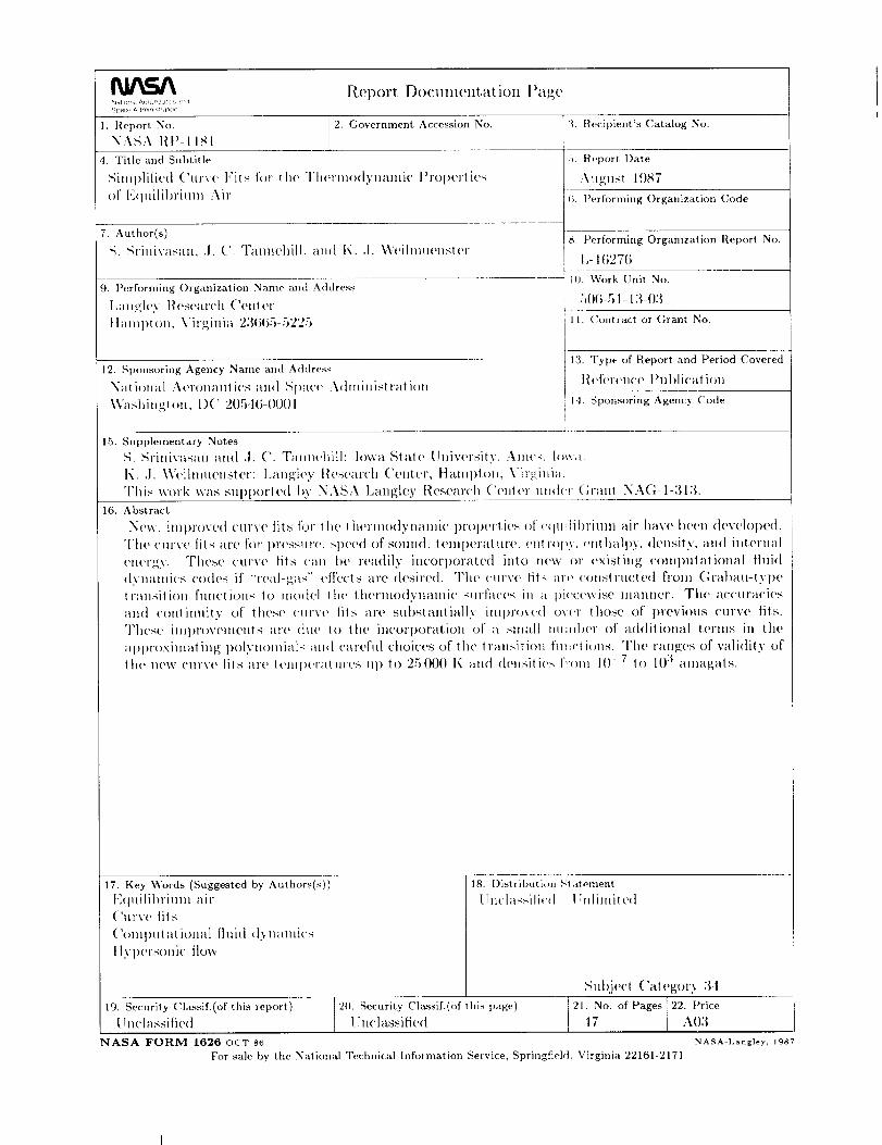
16. Abstract,

New, imt)rt)vetI curve tit_ for ilw therulo(tynamic l)roperlies t)I' (,quilit)rium air have Been (levclol)cd.

The ('mve ills are for l)rt'ssm'e. _,l)ec(I of sotm(t, t eml)erature, ('ntV()l)V, cut hall)y, tlensity, and iutcrnal

ener£y. These curve fits can t)(, rea(tily incorporated into n('_v or existing ('Oml)ulalional fluid

([3mmfi('s cotles if' "'r(,al-_as'" effects arc desire(I. The curve fits :tl[' (ou_tructc(l from Grat)au-typetr:msition fim('tious to model lh(' thcrmodynantic _url'a('es in a pi('c('wisc mamwr. The accm'acics

and ('()ulimtity of these ('urvc tils are substantially iml)rovutt ov('r those of previous CIlI'V( _ fitS.

These improvemeul._ are due It) the incori)oration of a small uuml)('r of a(hlitiomd terms in the

al)l)r()ximating polynomials and careful choices of the transition tmwt it)us. The ranges of validity ofthe new cttrvt, fits arc l(qnt)eratuvcs u l) to 25000 l( and (tt,nsitie- I'r,ml 10 -7 It) 10 ?' amagats.

17. Key Words (Suggested by Authors(s))Ettldlibrium air(htrve fits

('(mqmtatit)nal fluid (lymmlics

Ityl)t'r._tmic ttow

18. Distribution ,'_tatement

[in('la_itit'_t I ;nlimited

%ul)je('t Category 34

19. Security Classif.(of this report) 1 2(1. Security Cla.ssif.(of this page) 21. No. of Pages 22. Price

I!nclassiiiett 1 lrn('lassified _ 17 A0?,NASA FORM 1626 OCT 86 NASA-Langley, 1987

For sale by the National Technical hfformation Service, Springfield, Virginia 22161-2171