This article appeared in a journal published by Elsevier. The attached copy is furnished to the author for internal non-commercial research and education use, including for instruction at the authors institution and sharing with colleagues. Other uses, including reproduction and distribution, or selling or licensing copies, or posting to personal, institutional or third party websites are prohibited. In most cases authors are permitted to post their version of the article (e.g. in Word or Tex form) to their personal website or institutional repository. Authors requiring further information regarding Elsevier’s archiving and manuscript policies are encouraged to visit: http://www.elsevier.com/copyright
Transcript
This article appeared in a journal published by Elsevier. The attachedcopy is furnished to the author for internal non-commercial researchand education use, including for instruction at the authors institution
and sharing with colleagues.
Other uses, including reproduction and distribution, or selling orlicensing copies, or posting to personal, institutional or third party
websites are prohibited.
In most cases authors are permitted to post their version of thearticle (e.g. in Word or Tex form) to their personal website orinstitutional repository. Authors requiring further information
regarding Elsevier’s archiving and manuscript policies areencouraged to visit:
Theory of indentation on multiferroic composite materials
Weiqiu Chen a, Ernian Pan b,n, Huiming Wang a, Chuanzeng Zhang c
a Department of Engineering Mechanics, Zhejiang University, Yuquan Campus, Hangzhou 310027, PR Chinab Department of Civil Engineering and Department of Applied Mathematics, University of Akron, Akron, OH 44326-3905, USAc Department of Civil Engineering, University of Siegen, D-57068 Siegen, Germany
a r t i c l e i n f o
Article history:
Received 22 March 2010
Received in revised form
7 June 2010
Accepted 14 July 2010
Keywords:
Indentation
Half-space Green’s functions
Transverse isotropy
Magneto-electro-elastic
Multiferroic composite
a b s t r a c t
This article presents a general theory on indentation over a multiferroic composite half-
space. The material is transversely isotropic and magneto-electro-elastic with its axis of
symmetry normal to the surface of the half-space. Based on the corresponding half-space
Green’s functions to point sources applied on the surface, explicit expressions for the
generalized pressure vs. indentation depth are derived for the first time for the three
common indenters (flat-ended, conical, and spherical punches). The important multiphase
coupling issue is discussed in detail, with the weak and strong coupling being correctly
revisited. The derived analytical solutions of indentation will not only serve as benchmarks
for future numerical studies of multiphase composites, but also have important applications
to experimental test and characterization of multiphase materials, in particular, of
multiferroic properties.
& 2010 Elsevier Ltd. All rights reserved.
1. Introduction
Study on magneto-electro-elastic (MEE) and/or multiferroic materials/composites has recently emerged as animportant topic in various research communities because of the great potential applications of these materials andrelated devices to edge-cutting technologies (Spaldin and Fiebig, 2005; Nan et al., 2008). The multi-couplings amongelastic, electric and magnetic fields in multiferroic materials also present a challenge on the theoretical analysis associatedwith the magnetoelectric (ME) effect (Nan, 1994; Benveniste, 1995; Wu and Huang, 2000), effective properties ofcomposites (Li and Dunn, 1998), static and dynamic structural behaviors (Pan, 2001; Chen and Lee, 2003), fractures (Liuet al., 2001; Sih and Chen, 2003; Feng et al., 2007), Green’s functions and other mathematical aspects of the coupled theory(Pan, 2002; Wang and Shen, 2002; Li, 2003; Hou et al., 2005; X. Wang et al., 2008).
Indentation technique has been widely employed to characterize mechanical and/or electric properties of advanced andlayered materials (Lawn and Wilshaw, 1975; Gao et al., 1992; Kalinin and Bonnell, 2002; Vlassak et al., 2003; Kalinin et al.,2007b). This technique obviously relies on the solutions of the corresponding contact mechanics (Sneddon, 1965). Forearlier developments, readers are referred to Gladwell (1980), Johnson (1985) and Sackfield et al. (1993), to name a few. Asimple and conceptually straightforward method was also proposed by Yu (2001) for the study of various boundary-valueproblems (e.g. the frictionless normal indentation, prescribed surface tractions, sliding contact, and the adhesive punch) ina transversely isotropic half-space.
With the broad use of piezoelectric ceramics in various engineering applications, it is important to characterize theirmaterial properties. Giannakopoulos and Suresh (1999) presented a general theory of indentation of piezoelectricmaterials: they derived the relations between the generalized pressure and indentation depth by using the Hankel
Contents lists available at ScienceDirect
journal homepage: www.elsevier.com/locate/jmps
Journal of the Mechanics and Physics of Solids
0022-5096/$ - see front matter & 2010 Elsevier Ltd. All rights reserved.
Journal of the Mechanics and Physics of Solids 58 (2010) 1524–1551
Author's personal copy
transform for the three typical indenters as shown in Fig. 1. Giannakopoulos (2000) also used the indentation technique fordetermining the strength of piezoelectric materials. Concurrently, Chen and Ding (1999), Chen et al. (1999) and Chen(2000) conducted a series of investigations on the contact problems of spherical, conical and flat-ended punches on atransversely isotropic piezoelectric half-space by using Fabrikant’s method in potential theory (Fabrikant, 1989, 1991),which was further successfully used for the elastic solutions of several very important indentation problems by Hanson(1992a,b). They obtained the complete and exact three-dimensional (3D) expressions for the electroelastic field in thehalf-space in terms of elementary functions, and further found that, for conical and spherical indenters, although themechanical penetration does not induce a singular stress at the edge of contact, an additional application of a non-zeroconstant potential to the indenter would lead to a usual square-root singularity in the induced stress field at the edge ofcontact (Chen and Ding, 1999; Chen et al., 1999; Chen, 2000). This was later confirmed by Kalinin et al. (2004) andKarapetian et al. (2005), who employed the correspondence principle developed in Karapetian et al. (2002). However, sucha stress singularity phenomenon was not observed in Giannakopoulos and Suresh (1999) and Yang (2008), both employedthe Hankel transform. The difference between the results obtained by different methods is still unclear up to now.
Recently, J.H. Wang et al. (2008) presented an interesting study on the indentation of piezoelectric thin films by usingthe Hankel transform. They derived some useful empirical formulae based on comprehensive numerical simulations.Exciting works led by Kalinin (Kalinin et al., 2004; Karapetian et al., 2005; Kalinin et al., 2007b) have further shown theimportance of exact 3D contact solutions in interpreting quantitatively the responses of various scanning probemicroscopies (SPM). They recently considered the indentation of piezoelectric materials by flat and non-flat punches ofarbitrary planform (Karapetian et al., 2009).
Giannakopoulos and Parmaklis (2007) conducted a parallel study on piezomagnetic materials by employing the Hankeltransform. They showed that the coupling between the elastic and magnetic fields would lead to a significant effect on theindentation force. They also conducted an experimental study by using Terfenol-D material and compared both theirtesting results and theoretical predictions.
There are only a few works on contact mechanics of MEE or multiferroic materials. Hou et al. (2003) presented exactsolutions of elliptical Hertzian contact of MEE bodies for both smooth and frictional contact cases. Their work is an extension
P
undeformed surface
h2a
R
P
undeformed surface
h2a
P
undeformed surface
h2a
�
Fig. 1. Three common indenters: (a) a flat-ended circular punch, (b) a circular cone, and (c) a sphere. P denotes the total mechanical force, a the contact
radius, and h the indentation depth.
W. Chen et al. / J. Mech. Phys. Solids 58 (2010) 1524–1551 1525
Author's personal copy
of Hanson and Puja (1997) for the corresponding transversely isotropic elastic materials based on the method in potentialtheory developed by Fabrikant (1989). However, the results obtained in Hou et al. (2003), although mathematically beautiful,are somehow complicated because of the elliptical geometry considered. As such, some important issues related to themagnetoelectric properties of the indenter could not be addressed. For most applications, indenters are axisymmetric andusually have a much simpler shape than the elliptical one. Shown in Fig. 1 are the three common indenters, i.e. the flat-endedcylindrical punch, the conical punch and the spherical punch. With the rapid developments of multiferroic materials,structures and devices, it is hence very important to develop a theory on the contact mechanics between the indenters andmultiferroic materials, not to mention that the corresponding work on piezoelectric materials has already stimulated verybroad interests in research and applications (see, for example, Kalinin et al., 2007b).
Motivated by the potential broad and important applications of multiferroic materials and composites, we present inthis paper, the basic theory of indentation on these materials/composites. We first present the governing equations and thecorresponding half-space Green’s function of surface sources in transversely isotropic MEE materials in Section 2. InSection 3, we present the exact solutions for the three common indenters (flat-ended, conical, and spherical punches,see Fig. 1). The important multiphase coupling issue is analyzed through numerical examples and the reduced uncoupledresults are discussed in Section 4, contributing further on clarifying the controversial stress singularity issue at the contactedge. Finally in Section 5, we summarize our results and discuss also their potential future applications.
2. Governing equations and half-space Green’s function in transversely isotropic MEE materials
We introduce the cylindrical coordinates (r, y, z) with the r�y plane parallel to the plane of isotropy of the transverselyisotropic MEE material. The origin of the z-coordinate is on the surface and the z-axis points into the half-space. In thissystem, the generalized constitutive relations are (Chen et al., 2004)
where sij, Di, and Bi are the stresses, electric displacements, and magnetic inductions (i.e., magnetic fluxes), respectively;sij, Ei, and Hi are the strains, electric fields and magnetic fields, respectively; cij, eij, and mij are the elastic, dielectric, andmagnetic permeability coefficients, respectively; eij, qij, and dij are the piezoelectric, piezomagnetic, and magnetoelectriccoefficients, respectively. For the transversely isotropic material, we also have c66=(c11–c12)/2. It is obvious that variousdecoupled cases can be reduced from Eq. (1) by setting the appropriate coupling coefficients to zero. This, as well as theweakly and strongly coupled cases, will be addressed later.
The strain–elastic displacement, electric field-potential, and magnetic field-potential relations are
srr ¼@ur
@r, syy ¼
1
r
@uy
@yþ
ur
r, szz ¼
@uz
@z, syz ¼
1
2
@uy
@zþ
1
r
@uz
@y
� �,
srz ¼1
2
@uz
@rþ@ur
@z
� �, sry ¼
1
2
1
r
@ur
@yþ@uy
@r�
uy
r
� �, ð2aÞ
Er ¼�@f@r
, Ey ¼�1
r
@f@y
, Ez ¼�@f@z
, ð2bÞ
Hr ¼�@c@r
, Hy ¼�1
r
@c@y
, Hz ¼�@c@z
, ð2cÞ
where ui, f, and c are the elastic displacement, electric potential, and magnetic potential, respectively.In the cylindrical coordinate system, the generalized equilibrium equations for the system free of any body sources are
@srr
@rþ
1
r
@sry
@yþ@srz
@zþsrr�syy
r¼ 0,
@sry
@rþ
1
r
@syy
@yþ@syz
@zþ
2sry
r¼ 0,
W. Chen et al. / J. Mech. Phys. Solids 58 (2010) 1524–15511526
Author's personal copy
@srz
@rþ
1
r
@syz
@yþ@szz
@zþsrz
r¼ 0, ð3aÞ
@Dr
@rþ
1
r
@Dy
@yþ@Dz
@zþ
Dr
r¼ 0, ð3bÞ
@Br
@rþ
1
r
@By
@yþ@Bz
@zþ
Br
r¼ 0: ð3cÞ
If we assume that there is a vertical force P, point electric charge Q, and magnetic ‘‘charge’’ M (electric current) appliedat the origin on the surface, then the problem is axisymmetric with uy=0 and q/qy=0. Denoting P1=P, P2=�Q and P3=�M,we then find the point-source Green’s functions as (Hou et al., 2003, 2005)
urðr,zÞ ¼�X4
i ¼ 1
Air
RiR*i
, wkðr,zÞ ¼X4
i ¼ 1
aikAi1
Ri, szlðr,zÞ ¼�
X4
i ¼ 1
gilAizi
R3i
,
tzkðr,zÞ ¼�X4
i ¼ 1
giksiAir
R3i
, s2ðr,zÞ ¼ 2c66
X4
i ¼ 1
Air2
R2i R*
i
1
Riþ
1
R*i
!, ð4Þ
where k=1, 2, 3 and l=1, 2, 3, 4, Ri ¼
ffiffiffiffiffiffiffiffiffiffiffiffiffiffir2þz2
i
q, R*
i ¼ Riþzi, zj=sjz, and si (i=1, 2, 3, 4) are the four roots (eigenvalues) with
positive real parts, which are assumed distinct in this paper, of the characteristic equation given in Appendix A. For thecase of equal eigenvalues, its analysis is similar to Chen (2000) for piezoelectric materials. Furthermore, in writing thecompact solution (4), we have introduced the following notations:
where aij are defined in Appendix A, and the coefficients Ai in Eq. (4) are determined from the boundary conditions at z=0
as well as the generalized force equilibrium condition (Hou et al., 2003); they can be expressed as Ai ¼P3
j ¼ 1 IijPj, where
I1j
I2j
I3j
I4j
8>>>><>>>>:
9>>>>=>>>>;¼
1
2p
g11s1 g21s2 g31s3 g41s4
g11 g21 g31 g41
g12 g22 g32 g42
g13 g23 g33 g43
266664
377775
�1 0
d1j
d2j
d3j
8>>>><>>>>:
9>>>>=>>>>;
, ð7Þ
where dij is the Kronecker delta. It can be seen from Eq. (4) that the Green’s functions for point sources applied on theboundary of a half-space are expressed exactly and explicitly in terms of elementary functions. This will be greatlybeneficial to the succeeding analysis of contact problems.
Denoting xkj ¼P4
i ¼ 1 aikIij, we have the following important relation:
xkj ¼ xjk, ð8Þ
which can be verified by direct substitution. This result follows from the reciprocity theorem as presented in Appendix B.
3. Boundary value problems and fundamental results of indentation on a MEE half-space
3.1. Boundary conditions and integral expression
It is obvious that, for a given indentation problem, the field quantities should vanish at infinity. This has beenautomatically satisfied by the Green’s functions given in Eq. (4). Thus, only the conditions on the boundary surface z=0should be considered. As for the boundary value problems for the three common indenters shown in Fig. 1(a)–(c), wediscuss them separately in terms of their mechanical, electric, and magnetic conditions.
For the mechanical boundary conditions, we have
0rrra :
uzðr,0Þ ¼ h, for flat,
uzðr,0Þ ¼ h�r cotb, for cone,
uzðr,0Þ ¼ h�r2=ð2RÞ, for sphere,
8><>: ð9aÞ
W. Chen et al. / J. Mech. Phys. Solids 58 (2010) 1524–1551 1527
Author's personal copy
rZ0 : srzðr,0Þ ¼ 0, ð9bÞ
r4a : szzðr,0Þ ¼ 0, ð9cÞ
where h is the indentation depth, a the radius of the circular contact area, b the half apex angle of the conical indenter, andR the radius of the spherical indenter.
For the electric boundary conditions, we have for the three indenters:
(a) For a perfect electric conducting indenter with constant electric potential f0:
0rroa : fðr,0Þ ¼f0, r4a : Dzðr,0Þ ¼ 0: ð10Þ
(b) For an indenter as a perfect electric insulator with zero electric charge:
rZ0 : Dzðr,0Þ ¼ 0: ð11Þ
For the magnetic boundary conditions, we have, for the three indenters, similarly:
(a) For a perfect magnetic conducting indenter with constant magnetic potential c0:
0rroa : cðr,0Þ ¼c0, r4a : Bzðr,0Þ ¼ 0: ð12Þ
(b) For an indenter as a perfect magnetic insulator with zero magnetic flux:
rZ0 : Bzðr,0Þ ¼ 0: ð13Þ
By the method of superposition, the indentation (generalized) displacements (vertical elastic displacement, and electricand magnetic potentials) can be expressed in terms of integrals over the indenter area S (0rrra) of the unknownpressure distribution and the unknown or known electric charge or magnetic flux, which depends on the indenter’selectromagnetic properties, as discussed above. This leads to
wkðr,y,0Þ ¼X3
j ¼ 1
xkj
Z 2p
0
Z a
0
pjðr,y0Þ
R0rdrdy0 ðk¼ 1,2,3Þ, ð14Þ
where R0 is the distance between the two surface points (r, y, 0) and (r, y0, 0) defined as R0 ¼ffiffiffiffiffiffiffiffiffiffiffiffiffiffiffiffiffiffiffiffiffiffiffiffiffiffiffiffiffiffiffiffiffiffiffiffiffiffiffiffiffiffiffiffiffiffiffiffiffir2þr2�2rrcosðy�y0Þ
p, and
pkðr,yÞ ¼ �szkðr,y,0Þ ðk¼ 1,2,3Þ: ð15Þ
For axisymmetric problems, both wk and pk (k=1, 2, 3) are independent of the angle y. However, we still keep thisvariable in Eq. (14) so that the governing equations have the same structure as that in Fabrikant (1989, 1991), whoseresults then will be employed here. Also, occasionally we may write pk(r, y)=pk(r) or simply pk for brevity.
3.2. Solution for electrically and magnetically conducting indenters
First, we assume that all the three ‘‘pressures’’ pk (k=1, 2, 3) are unknowns, i.e. the indenter is electrically andmagnetically conducting. From Eq. (14), we obtainZ 2p
0
Z a
0
pjðr,y0Þ
R0rdrdy0 ¼
1
ZX3
k ¼ 1
Zkjwkðr,y,0Þ ð j¼ 1,2,3Þ ð16Þ
where Z=9xkj9 is the determinant, and Zkj are the corresponding cofactors. In view of Eq. (8), we have
Zkj ¼ Zjk: ð17Þ
The integral equations, Eq. (16), then can be solved using either the well-known property of Abel operator or theexisting results in the potential theory. Here we use the results of Fabrikant (1989) and Hanson (1992a,b). While we omitthe detailed derivation, some key steps are listed in Appendix C for easy reference. We remark that although a very similarderivation for piezoelectric materials can be found in Chen and Ding (1999), Chen et al. (1999), and Chen (2000), here inthis paper a different condition (i.e., total stress field vanishes at the contact edge) for the determination of the contactradius of the conical or spherical indenter is used, leading to a quite different result than that in Chen and Ding (1999) andChen et al. (1999) even for a piezoelectric material. This alternative condition was also employed by Giannakopoulos andSuresh (1999), Yang (2008), and J.H. Wang et al. (2008) for piezoelectric materials. After solving the integral equations (16),we can obtain the following important results for the three common indenters.
3.2.1. Flat indenter
The pressure, normal electric displacement, and normal magnetic flux distributions under the flat indenter are
pjðr,yÞ ¼Z1jhþZ2jf0þZ3jc0
p2Z1ffiffiffiffiffiffiffiffiffiffiffiffiffi
a2�r2p ð j¼ 1,2,3Þ: ð18Þ
W. Chen et al. / J. Mech. Phys. Solids 58 (2010) 1524–15511528
Author's personal copy
Note that szz(r, y, 0)=�p1(r), Dz(r, y, 0)=�p2(r) and Bz(r, y, 0)=�p3(r). As expected, for a flat indenter, the constantdisplacement, electric potential, and magnetic potential play a similar role. Just like the purely elastic case (Fabrikant,1989), the normal stress is infinite at the edge of the contact area (i.e. r=a), exhibiting a square-root singularity. The electricdisplacement and magnetic flux also have the same singularity at r=a.
The resultant indentation force, total electric charge, and total magnetic flux are
Pj ¼ 2pZ a
0pjðrÞr dr ¼
2aðZ1jhþZ2jf0þZ3jc0Þ
pZ ð j¼ 1,2,3Þ: ð19Þ
Note that the resultant indentation force P=P1, the total electric charge Q=�P2 and the total magnetic charge M=�P3 asintroduced in Section 2, Eq. (19) may be rewritten as
P
Q
M
8><>:
9>=>;¼
2a
p
Z11
ZZ21
ZZ31
Z
�Z12
Z�Z22
Z�Z32
Z
�Z13
Z�Z23
Z�Z33
Z
266666664
377777775
h
f0
c0
8><>:
9>=>;�
2a
pC
h
f0
c0
8><>:
9>=>;�G
h
f0
c0
8><>:
9>=>;: ð20Þ
Normally one can define the indentation stiffness as a variation ratio dP/dh at constant electric and magnetic potentials,and hence the element G11 represents just the indentation stiffness coefficient. Similarly, G12 corresponds to theindentation piezoelectric coefficient, G13 the indentation piezomagnetic coefficient, G22 the indentation dielectriccoefficient, G23 the indentation magnetoelectric coefficient, and G33 the indentation magnetic permeability coefficient.Thus, Eq. (20) provides various stiffness relations (or the global constitutive relations) of the indenter, and the matrixG¼ ½Gij� ¼ ð2a=pÞ½Cij� may be termed as the generalized indentation stiffness matrix. Note that such a definition ofgeneralized stiffness coefficients exactly follows Yang (2008), but is clearly different from that in Kalinin et al. (2004) andKarapetian et al. (2005) by the factor of 2a/p, which represents the geometric effect of the indenter. In fact, in thepiezoelectric case, the corresponding elements in C were used by Kalinin et al. (2004) and Karapetian et al. (2005) asvarious indentation constants. For the flat-ended indenter, either G or C can be seen as the indentation stiffness matrixsince the contact radius a is prescribed and does not change during indentation. From Eq. (17), we obtain the followingthree interesting relations:
C12 ¼�C21, C13 ¼�C31, C23 ¼ C32, ð21Þ
with the first one being observed by Kalinin et al. (2004) for a piezoelectric half-space, and proved later through a rathercomplicated derivation (Kalinin et al., 2007a). As mentioned earlier and detailed in Appendix B, these relations stem fromthe reciprocity pertinent to the linear theory of magneto-electro-elasticity. It is further interesting to note that, the factor2a/p also appears in the stiffness relations for any axisymmetric indenter. While this factor is fixed for a flat indenter, itvaries with the total force exerted on the conical or spherical indenter to be considered below and depends further on thematerial properties of the half-space.
The indentation depth is found as
h¼1
Z11
pZP
2a�ðZ21f0þZ31c0Þ
� �, ð22Þ
which is expressed in terms of the resultant force, and the prescribed electric and magnetic potentials. It is obtaineddirectly from the first equation in Eq. (19). From this relation, it is clear that the indentation depth can be convenientlyadjusted by imposing a proper electric or magnetic potential on the conducting indenter, a feature could be very useful inindentation test of multiferroic materials.
The complete and exact 3D expressions for the MEE field in the half-space are presented in Appendix D. These areparticularly useful in evaluating the material failure strength by the indentation technology, estimating the resolution ofelectromagnetic microscopy, or interpreting the polarization switching behavior in multiferroic materials (Kalinin et al.,2004), which is especially important in developing new devices of high-density and high-performance memories.
3.2.2. Conical indenter
The pressure, normal electric displacement, and normal magnetic flux distributions under the conical indenter are:
pjðrÞ ¼Z1j cotb
2pZcosh�1 a
r
� �þZ1jðh�pacotb=2ÞþZ2jf0þZ3jc0
p2Z1ffiffiffiffiffiffiffiffiffiffiffiffiffi
a2�r2p ð j¼ 1,2,3Þ, ð23Þ
Compared to the flat indenter (18), the conical indenter causes very different distributions of the pressure, normalelectric displacement and magnetic flux under the indenter since the conical shape induces a non-uniform mechanicalindentation. It is interesting to note, however, that the normal stress is no longer singular at r=a, as required in obtainingthe solution, see Appendix C. In fact, by utilizing the relation in Eq. (26) below, we obtain from Eq. (23) that
p1ðrÞ ¼Z11 cotb
2pZ cosh�1 a
r
� �,
W. Chen et al. / J. Mech. Phys. Solids 58 (2010) 1524–1551 1529
Author's personal copy
which gives p1(a)=0. On the other hand, a logarithmic singularity in the stress field appears at r=0 due to the sharpness ofthe conical apex (Hanson, 1992a; Chen et al., 1999). As for the electric and magnetic fields, they still exhibit the commonsquare-root singularity at r=a due to the discontinuity in the surface electric/magnetic potentials across the edge ofthe contact.
The resultant indentation force, total electric charge, and total magnetic flux are:
Pj ¼a
pZ Z1jhþ 2Z2j�Z1jZ21
Z11
� �f0þ 2Z3j�
Z1jZ31
Z11
� �c0
� �ð j¼ 1,2,3Þ, ð24Þ
which can also be rewritten in the form of Eq. (20), but with a different C matrix
C¼1
Z
1
2Z11
1
2Z21
1
2Z31
�1
2Z12
1
2
Z212
Z11
�Z22
1
2
Z12Z31
Z11
�Z32
�1
2Z13
1
2
Z21Z13
Z11
�Z23
1
2
Z231
Z11
�Z33
2666666664
3777777775: ð25Þ
The symmetry relations (21) still hold. In deriving Eq. (24), we have utilized the relation in Eq. (26) below. In spite of theadditional magnetic field, relation (24) looks just like that derived by Karapetian et al. (2005) for a piezoelectric half-space.However, even with proper degeneration procedures as outlined in Appendix E, our relation will not be identical to that inKarapetian et al. (2005) for the piezoelectric half-space since a different condition on vanishing stress singularity at thecontact edge is used here. It is also noted that, for the conical indenter, the contact radius a depends not only on the totalpressure, but also on the material properties of the half-space (see Eq. (27) below). From Eqs. (24) and (26), we cancalculate
dP
dh f0 ,c0
¼2aZ11
pZ,
dP
df0 h,c0
¼2aZ21
pZ,
dP
dc0 h,f0
¼2aZ31
pZ,
which show that the elements G11, G12 and G13 in matrix G coincide with the indentation coefficients defined above exceptfor a factor 2. However, further calculation shows that the other elements in G no longer bear the same physical essences asthose defined before. For example, we have
dQ
dh f0 ,c0
¼�2aZ12
pZ�
2
pZZ22�
Z212
Z11
� �f0þ Z32�
Z12Z31
Z11
� �c0
� �2
pcotb:
Thus, strictly speaking, the matrix G is not a generalized indentation stiffness matrix, neither the matrix C for a conical
indenter, according to the definition by Yang (2008). Nevertheless, we can still obtain the particular physical meanings ofother elements in matrix G. For example, we can find ðdQ=dhÞ9f0 ¼ 0,c0 ¼ 0 ¼ 2G21. Thus, under the condition of f0=c0=0, theelement G21 still corresponds to the commonly defined indentation coefficient except for a factor 2. In the following, forsimplicity, we therefore will treat the matrix G as a measure of related indentation coefficients as well. On the other hand,it may be inappropriate to simply treat the matrix C as the indentation stiffness matrix since the contact radius a alsodepends on the material properties of the half-space.
which indicates that the contact radius is solely determined by the total mechanical force, independent of the electric andmagnetic potentials. As shown in Appendix C, the relation (26) comes from the requirement that there is no singularity inthe total stress field at r=a, as is also the case in the elastic contact mechanics (Sneddon, 1965; Fabrikant, 1989). Whenf0=c0=0, we obtain h¼ pacotb=2, the same as that in Chen et al. (1999) and Karapetian et al. (2005) for the correspondingpiezoelectric material and in Hanson (1992a) for the elastic material.
The complete and exact 3D expressions for the MEE field in the half-space due to a conical indenter are also presentedin Appendix D.
1 For stable materials, we usually have Z11/Z40. This can be readily understood from the physical consideration that a pressure P will lead to contact
since no exclusive force is accounted in the present analysis. This is confirmed by the numerical calculation as presented in Section 4.
W. Chen et al. / J. Mech. Phys. Solids 58 (2010) 1524–15511530
Author's personal copy
3.2.3. Spherical indenter
The pressure, normal electric displacement, and normal magnetic flux distributions under the spherical indenter are
pjðrÞ ¼2Z1j
p2ZR
ffiffiffiffiffiffiffiffiffiffiffiffiffia2�r2
pþZ1jðh�a2=RÞþZ2jf0þZ3jc0
p2Z1ffiffiffiffiffiffiffiffiffiffiffiffiffi
a2�r2p ð j¼ 1,2,3Þ: ð28Þ
Unlike the flat or conical indenter, there is no singularity in the total stress field either at the edge r=a or the center r=0of the contact area.
The resultant indentation force, total electric charge, and total magnetic flux are
Pj ¼2a
pZ2
3Z1jhþ Z2j�
Z1jZ21
3Z11
� �f0þ Z3j�
Z1jZ31
3Z11
� �c0
� �ð j¼ 1,2,3Þ, ð29Þ
or in the form of Eq. (20), the matrix C now reads as
C¼1
Z
2
3Z11
2
3Z12
2
3Z13
�2
3Z12
Z212
3Z11
�Z22
Z12Z13
3Z11
�Z23
�2
3Z13
Z12Z13
3Z11
�Z23
Z213
3Z11
�Z33
2666666664
3777777775: ð30Þ
Again, the relation (29) is similar to that in Karapetian et al. (2005) for a piezoelectric half-space, but it cannot bereduced to that due to the different assumptions employed.
The indentation depth is
h¼a2
R�Z21f0þZ31c0
Z11
, ð31Þ
where a is determined from Eq. (29) for j=1 as follows:
It is noted that relation (31) also comes from the requirement of no singularity in the total stress field at r=a, as shownin Appendix C.
The complete and exact 3D expressions for the MEE field in the half-space due to a spherical indenter are given inAppendix D.
3.3. Solution for electrically conducting and magnetically insulating indenters
Second, we assume that the indenter is electrically conducting but magnetically insulating. From Eq. (14), we can obtain
wkðr,y, 0Þ ¼X2
j ¼ 1
xkj
Z 2p
0
Z a
0
pjðr,y0Þ
R0rdrdy0 ðk¼ 1,2,3Þ: ð33Þ
Then from the first two equations of (33), we obtainZ 2p
0
Z a
0
p1ðr,y0Þ
R0rdrdy0 ¼
1
Z33
x22w1ðr,y,0Þ�x12w2ðr,y,0Þ �
, ð34aÞ
Z 2p
0
Z a
0
p2ðr,y0Þ
R0rdrdy0 ¼
1
Z33
�x21w1ðr,y,0Þþx11w2ðr,y,0Þ �
: ð34bÞ
Obviously, the above two integral equations have the same structure as those in Eq. (16), and hence exact solutions forthe three common types of indenters can be derived following a similar procedure. On the other hand, the magneticpotential can be obtained from the third in Eq. (33) without solving any integral equation as
w3ðr,y, 0Þ ¼ �1
Z33
Z13w1ðr,y, 0ÞþZ23w2ðr,y, 0Þ �
ð0rrraÞ: ð35Þ
This solution can also be obtained directly from Eq. (16) for j=3 and p3=0.
3.3.1. Flat indenter
The pressure and normal electric displacement distributions under the flat indenter are
The magnetic potential distribution under the spherical indenter is
w3ðr,y, 0Þ ¼ �1
Z33
Z13 h�r2
2R
� �þZ23f0
� �ð0rrraÞ: ð52Þ
3.4. Magnetically conducting and electrically insulating indenters
If the indenter is magnetically conducting but electrically insulating, then the analysis is very similar to that justdescribed above and hence is omitted here. More specifically, to find the solutions for this case, one needs only simply tointerchange the electric (magnetic) and magnetic (electric) quantities in the solutions given in Section 3.3.
3.5. Electrically and magnetically insulating indenters
We now assume that the indenter is both electrically and magnetically insulating. From Eq. (14), we obtain
wkðr,y, 0Þ ¼ xk1
Z 2p
0
Z a
0
p1ðr,y0Þ
R0rdrdy0 ðk¼ 1,2,3Þ: ð53Þ
When k=1, the above equation givesZ 2p
0
Z a
0
p1ðr,y0Þ
R0rdrdy0 ¼
1
x11w1ðr,y,0Þ: ð54Þ
The exact solutions for the three common types of indenters then can be readily obtained by using the results ofFabrikant (1989, 1991) and Hanson (1992a,b). The electric and magnetic potentials can be obtained from Eq. (53) as
The electric and magnetic potentials under the indenter are
wkðr,y,0Þ ¼xk1
x11h�
r2
2R
� �ðk¼ 2,3; 0rrraÞ: ð72Þ
W. Chen et al. / J. Mech. Phys. Solids 58 (2010) 1524–15511534
Author's personal copy
4. Numerical results and discussion
A complete set of material properties of single-phase multiferroic materials (such as Cr2O3, BiFeO3, YMnO3, LuFe2O3,etc.) cannot be found in literature. Hence, we confine ourselves to the MEE composite materials made of piezoelectric andmagnetostrictive phases. The material properties of piezoelectric ceramic BaTiO3 and those of piezomagnetic crystallineCoFe2O4 are chosen for the following numerical illustrations, and they are given in Tables 1 and 2, where all the absentmaterial constants equal zero. It then becomes obvious that, there is no direct ME effect in either phase, but the compositedoes exhibit the ME coupling due to the so-called product property of the composite through the mechanical straininteraction.
The material properties of the composite are estimated using the simple rule of mixture according to the volumefractions (Sih and Chen, 2003). Denoting for the composite the volume fraction of CoFe2O4 as x, and that of BaTiO3 as 1�x,we then have
MC ¼MEð1�xÞþMMx, ð73Þ
where M represents an arbitrary material constant, and the subscripts C, E, and M indicate the composite, piezoelectricphase and piezomagnetic phase, respectively.
In the following, we consider five different cases of material combinations, by taking the volume fraction of CoFe2O4 asx=0, 0.25, 0.5, 0.75, and 1, respectively. Obviously, when x=0, the composite is purely piezoelectric, whilst x=1 correspondsto a purely piezomagnetic material. Various degeneration cases are discussed in Appendix E. Among many differentcombinations of material constants appearing in matrices C and G, which vary with the geometry and magnetoelectricproperty of the indenter, xij (i, j=1, 2, 3) are the most fundamental. These and the associated parameters Zij, the cofactors of[xij] are listed in Table 3 for the five values of the volume fraction x.
Table 3 shows that the parameter x23, which is associated with the ME effect or coupling during indentation, is not zerowhen xa0. This clearly attributes to the product property of the composite which in turn is caused by the mechanicalstrain interaction. Thus, the indentation technique can be used to characterize the ME effect in composites or crystals.From this table, it is also seen that the two parameters x22 and x33, which in certain sense correspond to the dielectric andmagnetic properties respectively, vary with the volume fraction more significantly than the other parameters. Theirvariations with the volume fraction x are shown in Fig. 2. When the electric (or magnetic) field tends to decouple from themagneto-elastic (or electro-elastic) coupled field, x22 (or x33) increases rapidly, and finally arrives at the value ofx22 ¼�1=ð2p ffiffiffiffiffiffiffiffiffiffiffiffiffie11e33
We first assume that the flat-ended circular indenter is electrically and magnetically conducting (Case A). As discussedin Section 3, when the indenter is flat-ended, either the matrix G or C can be a direct measure of various stiffnesscoefficients related to the indentation process. For instance, we choose matrix C which can be expressed as
C¼
1 0 0
0 �1 0
0 0 �1
264
3751
ZZij
h i¼
1 0 0
0 �1 0
0 0 �1
264
375½xij�
�1
Table 1Material coefficients of the piezoelectric BaTiO3 (Pan, 2001). (cij in 109 N/m2, eij in C/m2, eij in 10�9 C2/(N m2), mij in 10�6 N s2/C2).
c11 c12 c13 c33 c44 c66
166 77 78 162 43 44.5
e31 e33 e15
�4.4 18.6 11.6
e11 e33 m11 m33
11.2 12.6 5 10
Table 2Material coefficients of the magnetostrictive CoFe2O4 (Pan, 2001). (cij in 109 N/m2, qij in N/(A m), eij in 10�9 C2/(N m2), mij in 10�6 N s2/C2).
c11 c12 c13 c33 c44 c66
286 173 170.5 269.5 45.3 56.5
q31 q33 q15
580.3 699.7 550
e11 e33 m11 m33
0.08 0.093 590 157
W. Chen et al. / J. Mech. Phys. Solids 58 (2010) 1524–1551 1535
Author's personal copy
Hence, one can easily compute matrix C once matrix [xij] is calculated. Table 4 lists the algebraic values of matrix C forthe five different material combinations.
It is observed from Table 4, the indentation elastic stiffness C11 increases with the volume fraction x. This is consistentwith the fact that the piezomagnetic phase CoFe2O4 is stiffer than the piezoelectric phase BaTiO3. Also as expected, withincreasing x, the indentation piezoelectric coefficient C12 decreases but the indentation piezomagnetic coefficients C13
increases. However, no monotonic variation of the indentation ME coefficient C23 can be observed. The complete spectrumof its variation with the volume fraction is shown in Fig. 3, which indicates that the indentation ME coefficient C23 arrivesat its maximum around x=0.5. This is physically reasonable as both phases play a somewhat equal role at such a volumefraction and the mechanical strain interaction between the two phases is optimized (Petrov and Srinivasan, 2008; Pan andWang, 2009).
For comparison, the values of the matrix C for other three cases, (i.e. Case B: electrically conducting and magneticallyinsulating, Case C: electrically insulating and magnetically conducting, and Case D: electrically and magneticallyinsulating), are summarized in Table 5. It should be noted that for Case D, although the only non-zero element in matrix Cis C11, it is not identical to the elastic case. To make such a comparison, we denote Case E as the purely elastic case wherethe elastic field is fully decoupled from the electric and magnetic fields. Then, we can calculate according to Fabrikant(1989)
Case E : C11 ¼ 3:96226, 4:25823, 4:52352, 4:76784, 4:99705ð1011 N=m2Þ
Table 3Basic indentation parameters for different material combinations.a
volume fraction x [xij] Z=9xij9b [Zij]
0.00 2:16825 1:76207 0
�1:04710 0
sym: �22:5079
264
375
�2.58086 –
0.25 2:08613 1:76439 1:95380
�1:48486 2:71289
sym: �1:88746
264
375
6.44020 2:80188 3:33553 3:37978
�3:94131 �2:21216
sym: �0:340891
264
375
0.50 2:03552 1:77480 1:93900
�2:35928 2:85507
sym: �1:00418
264
375
5.14794 2:36834 1:78776 5:08136
�2:04779 �2:37022
sym: �0:511736
264
375
0.75 2:00607 1:77755 1:89271
�4:94527 2:89808
sym: �0:683397
264
375
7.01360 3:37875 1:22026 9:87511
�1:37452 �2:44936
sym: �1:02365
264
375
1.00 1:98978 0 1:85696
�184:516 0
sym: �0:517441
264
375
�1.03304 –
a Units: x11 in 10�12 m2/N, x12 in 10�3 m2/C, x13 in 10�6 mA/N, x22 in 107 N m2/C2, x23 in 103 V A/N, x33 in 103 A2/N; Z in 10�2 m4 A2/(N C2); Z11 in
1010 m2 A2/C2, Z12 in m2 A2/(C N), Z13 in 101 m3 A/C2, Z22 in 10�9 m2 A2/N2, Z23 in 10�9 m3 A/(N C), Z33 in 10�4 m4/C2.b For volume fraction x=0 of CoFe2O4, Z=9xij9 (i,=1,2), the unit is 10�5 m4/C2; and for x=1, Z=9xij9 (i, j=1, 3), the unit is 10�9 m2 A2/N2.
-200
-160
-120
-80
-40
00
-250
-200
-150
-100
-50
0
Dielectric
Magnetic
ξ 22
(107 N
m2 /C
2 )
Volume fraction x
0.1 0.2 0.3 0.4 0.5 0.6 0.7 0.8 0.9 1
ξ 33
(102 A
2 /N)
Fig. 2. Variation of x22 and x33 with volume fraction x of CoFe2O4.
W. Chen et al. / J. Mech. Phys. Solids 58 (2010) 1524–15511536
Author's personal copy
for x=0, 0.25, 0.50, 0.75 and 1.00, respectively. Therefore, we observe that the indentation stiffness C11 varies with theelectromagnetic properties of the indenter, and in general for xa0, we have
Case D4Case C4Case B4Case A4Case E
In other words, among the five cases, the purely elastic case has the smallest C11! When the elastic field in the materialcouples with the electric or magnetic field, the well-known piezoelectric (or piezomagnetic) stiffening effect plays animportant role. The stiffening effect is more obvious when the indenter is electrically (or magnetically) insulating thanwhen it is electrically (or magnetically) conducting.
When x=0, the magnetic field in the material decouples from the coupled electro-elastic field. In this case, themagnetically insulating indenter will lead to a null magnetic field in the half-space, and exerts no effect on the electro-elastic field. Similarly, when x=1, for which the electric field becomes independent of the coupled magneto-elastic field inthe half-space, a change in the electric property of the indenter does not affect the magneto-elastic field.
The relative difference of the indentation stiffness coefficient C11 between Case D and Case E, defined as RD=(CaseD�Case E)/Case E, can be calculated as
RD¼ 16:40%, 12:57%, 8:60%, 4:55% and 2:86%
for x=0, 0.25, 0.50, 0.75 and 1.00, respectively. It is seen that for the pure piezoelectric material BaTiO3 (x=0), the differencebetween the (piezoelectric) coupled theory and the elastic theory is significant, and the coupled theory should be utilizedto interpret the indentation results. For the pure piezomagnetic material CoFe2O4 (x=1), the difference by using the elastictheory is around 3%. Thus, the feasibility of using the relatively simple elasticity theory to characterize the materialproperties of piezoelectric, piezomagnetic or multiferroic materials depends significantly on the coupling among variousfields in the materials. Simulations based on the completely coupled theory should be performed to evaluate the accuracyof various simplified models.
Table 4Matrix C for an electrically and magnetically conducting flat-ended indenter.a
Volume fraction x C Volume fraction x C
0.00 4:05716 6:82744 0
�6:82744 8:40128 0
0 0 0:444288
264
375
0.75 4:81742 1:73985 14:0799
�1:73985 1:95980 3:49230
�14:0799 3:49230 14:5953
264
375
0.25 4:35061 5:17923 5:24794
�5:17923 6:11985 3:43493
�5:24794 3:43493 5:29318
264
375
1.00 5:00890 0 17:9756
0 0:0541958 0
�17:9756 0 19:2614
264
375
0.50 4:60055 3:47276 9:87067
�3:47276 3:97789 4:60422
�9:87067 4:60422 9:94060
264
375
a Units: C11 in 1011 N/m2, C12, C21 in 101 C/m2, C13, C31 in 102 N/(mA), C22 in 10�8 C2/(N m2), C23, C32 in10�8 N/(V A), C33 in 10�4 N/A2.
0
1
2
3
4
5
0
C23
(10
-8 N
/ (V
A))
0.1 0.2 0.3 0.4 0.5 0.6 0.7 0.8 0.9 1
Volume fraction x
Fig. 3. Variation of the indentation ME coefficient with volume fraction x.
W. Chen et al. / J. Mech. Phys. Solids 58 (2010) 1524–1551 1537
Author's personal copy
Fig. 4 shows the pressure distribution under the flat-ended indenter for the five different cases discussed. The volumefraction is fixed at x=0.5. The dimensionless mechanical penetration h/a, electric potential f0
p=a are taken to be 0.1, 1 and 0.5, respectively. For all the five cases, the pressure tends to infinity at
the contact edge (r=a), exhibiting a usual square-root singularity as shown by Eq. (18), (36), or (56). It is clear that, inaddition to the mechanical penetration, different electric and magnetic potentials may be applied so that the magnitude ofthe pressure under the indenter can be adjusted. Similar observation can also be made with regard to the electricdisplacement and normal magnetic flux distributions under the indenter. In fact, the magnitude of any physical fieldvariable at a point in the multiferroic half-space can also be controlled by the mechanical, electric or magnetic means dueto the coupling among the three fields. This feature will be further discussed for a spherical indenter to be considered later.
4.2. Conical indenter
With the basic material parameters of the indentation given in Table 3, one can easily obtain the matrix C for a conicalor spherical indenter. The discussions will be similar to those for the flat-ended indenter, and hence are omitted here.Below, however, we pay our attention to other two important issues.
0
0.5
1
1.5
2
0
Case A
Case B
Case CCase DCase E
p 1 /c
44B
0.1 0.2 0.3 0.4 0.5 0.6 0.7 0.8 0.9 1
r/a
Fig. 4. Distribution of dimensionless pressure (p1/c44B) under the flat-ended indenter where h/a=0.1, f0
subscript B indicates the material constant of BaTiO3. The volume fraction of CoFe2O4 phase in the composite is x=0.5.
Table 5Matrix C for a flat-ended indenter under different electric and magnetic boundary conditions over the MEE half-space composite with different volume
fraction x.a
Volume
fraction x
C
Case B: Electrically conducting, magnetically
insulating
Case C: Electrically insulating, magnetically
conducting
Case D: Electrically and magnetically
insulating
0.00 4:05716 6:82744 0
�6:82744 8:40128 0
0 0 0
264
375
4:61201 0 0
0 0 0
0 0 0:444288
264
375
4:61201 0 0
0 0 0
0 0 0
264
375
0.25 4:35581 5:17583 0
�5:17583 6:11963 0
0 0 0
264
375
4:78892 0 4:95724
0 0 0
�4:95724 0 5:29298
264
375
4:79357 0 0
0 0 0
0 0 0
264
375
0.50 4:61035 3:46819 0
�3:46819 3:97768 0
0 0 0
264
375
4:90373 0 9:46872
0 0 0
�9:46872 0 9:94007
264
375
4:91275 0 0
0 0 0
0 0 0
264
375
0.75 4:83100 1:73648 0
�1:73648 1:95972 0
0 0 0
264
375
4:97188 0 13:7699
0 0 0
�13:7699 0 14:5946
264
375
4:98487 0 0
0 0 0
0 0 0
264
375
1.00 5:02568 0 0
0 0:0541958 0
0 0 0
264
375
5:00890 0 17:9756
0 0 0
�17:9756 0 19:2614
264
375
5:02568 0 0
0 0 0
0 0 0
264
375
a Units: C11 in 1011 N/m2, C12, C21 in 101 C/m2, C13, C31 in 102 N/(mA), C22 in 10�8 C2/(N m2), C23, C32 in 10�8 N/(V A), C33 in 10�4 N/A2.
W. Chen et al. / J. Mech. Phys. Solids 58 (2010) 1524–15511538
Author's personal copy
First, let us examine the element G11=aZ11/Z of the matrix G, which equals half of the indentation stiffness coefficient ofan electrically and magnetically conducting conical indenter as shown in Section 3. The contact radius a varies with thetotal pressure according to Eq. (27). Thus, the indentation stiffness coefficient varies with the total pressure, as shown inFig. 5. This is somewhat different from Kalinin et al. (2004) due to the fact that a different definition of the stiffnesscoefficient (Yang, 2008) has been employed here. In particular, if we take C11 as the indentation stiffness coefficient byfollowing Kalinin et al. (2004), we will then obtain a constant stiffness coefficient, which could not be obtained directlyfrom the experimental P–h curves. Comprehensive discussion also can be made on other elements of the matrix G, orvarious indentation coefficients strictly defined according to Yang (2008) and on the other conditions such as various MEproperties of the indenter.
Second, let us look at the difference of the pressure distribution under the indenter caused by different conditionsconcerning with the vanishing stress singularity at the contact edge (r=a), see further discussions presented in Appendix C.For convenience, Condition 1 is referred to the requirement that only the mechanically induced stress is non-singular atr=a, while Condition 2 corresponds to the case where there should be no singularity in the total stress at r=a. For anelectrically and magnetically conducting conical indenter, the distributions of the dimensionless pressure p1/c44B (withsubscript B for the material constant of BaTiO3) are shown in Fig. 6 for the two conditions when the volume fraction ofCoFe2O4 phase in the multiferroic half-space equals x=0.5. When Condition 1 is used, the pressure distribution apparentlydepends on the applied electric and magnetic potentials, and three combinations of them are considered. As indicated inthe figure, the first and second numbers in parentheses for Condition 1 are the dimensionless electric and magneticpotentials, defined by f0
p=a, respectively. The dimensionless radial coordinate r/a is used in
the figure, and it should be remembered that, unlike the flat-ended indenter, here a is not a constant, and will be differentfrom each other for the four curves in the figure (three curves for Conditions 1 and one curve for Condition 2). Also, thepenetration depth h is not specified in the figure; it actually relates to the total mechanical force as well as the electric andmagnetic potentials through Eqs. (26) and (27). As can be seen from the figure, the pressure does not tend to infinity at r=a
when Condition 2 is employed. Use of Condition 1, however, will induce a pressure having a square-root singularity at thecontact edge, unless f0=c0=0, for which the result becomes identical to that for Condition 2. Although it seems thatCondition 2 is physically more reasonable than Condition 1, delicate experiments are especially desired to justify it.
4.3. Spherical indenter
For a spherical indenter, here we confine ourselves to the induced MEE field in the half-space. The exact 3D expressions arepresented in Appendix D. It can be observed from there that the solutions are expressed in terms of elementary functions, thusgreatly facilitating our computation as well as future applications. The calculations are performed for an electrically andmagnetically conducting spherical indenter on a multiferroic half-space with the volume fraction of the piezomagnetic phasebeing fixed at x=0.5. Shown in Fig. 7 are the distributions of some dimensionless physical quantities along the axisymmetric
0
100
200
300
400
500
600
700
800
0
x = 0.0x = 0.25
x = 0.50
x = 0.75
x = 1.00G
11 (
N/m
)
P (μN)
0.05 0.1 0.15 0.2
Fig. 5. G11 for an electrically and magnetically conducting conical indenter with b=151.
W. Chen et al. / J. Mech. Phys. Solids 58 (2010) 1524–1551 1539
Author's personal copy
axis z (or r=0). The total dimensionless mechanical force is specified as P=ðc44BR2Þ ¼ 10�5, while three combinations of theelectric and magnetic potentials, (0,0), (1.0,0.5), and (0.5,1.0), are considered, both being in dimensionless form defined byf0
p=R, respectively. All the results are obtained by using Condition 2, as noticed above. Thus,
the contact radius is solely determined by the total mechanical force once the material of the half-space is specified, as seenfrom Eq. (32), and the mechanical penetration depth h is then determined from Eq. (31).
As shown in Fig. 7, when both the electric and magnetic potentials vanish, all the physical field variables also seem todisappear. However, this is not the case; in fact, their magnitudes are very small when compared to those for the othercases. To make it clear, we display in Figs. 8(a) and (b), respectively, the distribution of the axial displacement uz(0, z)/R andthat of the normal stress szz(0, z)/c44B for f0=c0=0 only. As mentioned earlier, the results for Condition 1 and Condition 2are the same in this particular case. Therefore, Fig. 7 illustrates that the difference of the MEE fields in the half-spacebetween the two different conditions could be substantial, which of course depends on the magnitudes of electric andmagnetic potentials applied on the indenter. For example, by comparing Fig. 7(a) with Fig. 8(a), it is seen that the verticaldisplacement induced by the mechanical force only is positive as expected, while when the electric and magneticpotentials are applied on the indenter and Condition 2 is used, the vertical displacement could be negative, which can alsobe seen from Eq. (31). Such characters may be utilized to experimentally determine what kind of condition (Condition 1,Condition 2, or other possible alternatives) should be employed in the analysis.
A common feature that can be observed from Figs. 7 and 8 is that all physical variables diminish rapidly with depth. Thisis identical to the physical nature of the problem, and also can be explicitly seen from the analytical solutions given inAppendix D. Of particular interest is the distribution of the normal stress component szz in Fig. 7(d). For the two potentialcombinations (1.0,0.5) and (0.5,1.0), the stress first changes from a small negative value to a maximum negative value,then increases until the maximum tensile value is reached, and eventually diminishes with increasing depth. Thus, themaximum tensile stress occurs at a certain depth under the indenter. The results shown in Fig. 7(d) also indicate thatthe stress field in the half-space can be conveniently controlled through the electric or magnetic means or both. It is notedthat, since Condition 1 is employed, szz is the same for all the three different cases of potential combinations. This can beeasily seen from Eqs. (28) and (31) that the pressure under the indenter is independent of the electric and magneticpotentials.
With regard to the distribution of the radial stress component srr or the circumferential stress component syy, asimilar but relatively simpler variation can be seen from Fig. 7(g). Note that these two stress components are equal at r=0which means physically there is no preferential direction and all normal stress components should be identical sincethe r�y plane is a plane of isotropy for the transversely isotropic multiferroic materials considered in this paper.Their equivalence could also be verified mathematically based on the exact expressions given in Eqs. (D5) and (D8)of Appendix D, from which we obtain sI
2 ¼ sII2 ¼ 0 by carrying out the limit r-0. The maximum tensile radial
(or circumferential) stress also occurs at a certain depth under the indenter, but it is closer to the surface than that forthe stress component szz. These tensile stress locations could potentially initiate a crack (it is of course also relatedto the fracture criterion, and actually, the maximum stress may occur at a place deviating from the axisymmetric axis, e.g.Ding et al., 2006).
From Figs. 7(b) and 7(c), we can see that the calculated electric and magnetic potentials coincide with the prescribedvalues at the surface. This, in certain sense, verifies our analytical solutions.
p=a, respectively. The subscript B indicates the material constant of BaTiO3. The volume fraction of CoFe2O4 phase in the
multiferroic half-space equals 0.5.
W. Chen et al. / J. Mech. Phys. Solids 58 (2010) 1524–15511540
Author's personal copy
0
0.02
0.04
0.06
0.08
0.1
-0.25
(0,0)(1.0,0.5)(0.5,1.0)
0
0.02
0.04
0.06
0.08
0.1
0
(0,0)(1.0,0.5)(0.5,1.0)
0
0.02
0.04
0.06
0.08
0.1
(0,0)(1.0,0.5)(0.5,1.0)
0
0.02
0.04
0.06
0.08
0.1
-1
(0,0)(1.0,0.5)(0.5,1.0)
0
0.02
0.04
0.06
0.08
0.1
0
(0,0)(1.0,0.5)(0.5,1.0)
0
0.02
0.04
0.06
0.08
0.1
0
(0,0)(1.0,0.5)(0.5,1.0)
uz (0, z)/R
-0.2 -0.15 -0.1 -0.05 0
z/R
z/R
� (0, z) �33B / c44B / R
� (0, z) �33B / c44B / R
0.2 0.4 0.6 0.8 1 1.2
0 0.2 0.4 0.6 0.8 1 1.2 0 1 2 3 4 5
�zz (0, z) / c44B
Dz (0, z) / e33B
5 10 15 20 25 30 35 40
Bz (0, z) / q33C
100 200 300 400 500 600 700 800
z/Rz/R
z/R
z/R
0
0.02
0.04
0.06
0.08
0.1
0
(0,0)
(1.0,0.5)
(0.5,1.0)
z/R
0.5 1 1.5 2 2.5 3 3.5 4 4.5 5
�rr, �� (0, z) / c33B
Fig. 7. Distributions of some dimensionless physical quantities along the axisymmetric axis in the multiferroic half-space (x=0.5) when it is pressed by an
electrically and magnetically conducting spherical indenter with a prescribed total force P=ðc44BR2Þ ¼ 10�5: (a) uz(0, z)/R, (b) fð0,zÞffiffiffiffiffiffiffiffiffiffiffiffiffiffiffiffiffiffiffiffie33B=c44B
C indicate the material constant of BaTiO3 and CoFe2O4, respectively.
W. Chen et al. / J. Mech. Phys. Solids 58 (2010) 1524–1551 1541
Author's personal copy
5. Conclusions
In this paper, we have presented a unified fundamental theory to deal with the contact problem between a rigid punch(or indenter) and a multiferroic half-space. The indenter may have a flat-ended, conical or spherical shape, and may beelectrically and magnetically conducting, electrically conducting and magnetically insulating, electrically insulating andmagnetically conducting, or electrically and magnetically insulating. Complete results are obtained by making use of theGreen’s function solution of the multiferroic half-space and the most recently extended method in potential theory(Fabrikant, 1989, 1991; Hanson, 1992a,b). In particular, exact 3D expressions for the coupled MEE fields in the half-spaceare presented in terms of elementary functions. The physical quantities on the surface of the multiferroic half-space inexact closed forms are also given as special cases.
Discussion is made on the particular condition for vanishing stress singularity at the edge of the spherical or conicalindenter. As opposed to the previous one where the mechanically induced part is assumed to be non-singular at thecontact edge, this paper assumes that the total stress field has no singularity there. We show that the results for the twodifferent conditions become identical when the electric potential and/or magnetic potential are zero (here ‘and/or’ dependson the magnetoelectric properties of the indenter). A detailed discussion is given for the piezoelectric materials, whichclearly identifies the differences in existing literature.
Apart from the piezoelectric materials, various other decoupled cases are also discussed (see Appendix E). For example,the solution for the piezomagnetic materials can be easily derived from that for the piezoelectric materials since the
0
0.02
0.04
0.06
0.08
0.1
0
0
0.02
0.04
0.06
0.08
0.1
-0.03
z/R
uz (0, z)/R×104
0.2 0.4 0.6 0.8 1 1.2 1.4 1.6 1.8
-0.025 -0.02 -0.015 -0.01 -0.005 0
�zz (0, z) / c44B
z/R
Fig. 8. Distributions of uz(0, z)/R and szz(0, z)/c44B for f0=c0=0 with all other parameters being the same as those in Fig. 7.
W. Chen et al. / J. Mech. Phys. Solids 58 (2010) 1524–15511542
Author's personal copy
magnetic field plays almost the same role as the electric field. Thus, various important discussions related to piezoelectricmaterials, e.g. on the piezoresponse force microscopy (Kalinin et al., 2004) can be directly borrowed and applied to thepiezomagnetic materials.
Some numerical examples are also presented for illustrations. Our results indicate that a complete coupling theoryshould be used for an accurate prediction of the indentation response, which can be used to characterize the materialproperties. Our results also show that the coupling among the magnetic, electric and elastic fields provide more feasibleways in controlling the magnitude as well as the distribution of various physical fields in the half-space. This interestingfeature could stimulate important applications of advanced technologies such as magnetically writing and electricallyreading memory, atomic force microscopy based micro-painting, and ferroelectric/ferromagnetic domain switch.
Acknowledgements
This work was supported by NSFC (Nos. 10725210 and 10832009). It was also partially supported by Air Force Office ofScientific Research under grant AFOSR FA9550-06-1-0317. Financial support from the German Research Foundation (DFG,Project-Nos.: ZH15/14-1 and ZH 15/15-1) is also acknowledged.
Appendix A. The related material coefficients
The four characteristic roots si (with real parts) are the solutions of the following eigenequation (Chen et al., 2004):
and P and G being the determinants of, Pij and Gij being the cominors of, the corresponding matrices P and C defined by
P¼
c33 e33 q33
�e33 e33 d33
�q33 d33 m33
264
375, C¼
c44 e15 q15
�e15 e11 d11
�q15 d11 m11
264
375:
The eigenequation (A1) includes the decoupled piezoelectric, piezomagnetic, and elastic materials as its special cases.For example, by setting qij=dij=0, along m33=0 and m11=1 (to remove the eigenvalues associated with the decoupledmagnetic field so that the size of the eigenequation is properly reduced) we obtain from Eq. (A2),
n0 ¼ 0, n1 ¼ c44ðc33e33þe233Þ,
n2 ¼ c44ðc33e11þe33e15Þþ½c11c33þc244�ðc13þc44Þ
2�e33þðe15þe31Þ
2c33þ½c11e33þc44e15�2ðc13þc44Þðe15þe31Þ�e33,
n3 ¼ c44ðc44e11þe215Þþ½c11c33�ðc13þc44Þ
2�e11þ½c11e33þðe15þe31Þ
2�c44þ2½c11e33�ðc13þc44Þðe15þe31Þ�e15,
n4 ¼ c11ðc44e11þe215Þ: ðA3Þ
Thus, Eq. (A1) becomes
n1s6�n2s4þn3s2�n4 ¼ 0, ðA4Þ
W. Chen et al. / J. Mech. Phys. Solids 58 (2010) 1524–1551 1543
Author's personal copy
which is identical to Eq. (5) in Chen (2000) for piezoelectric materials. Similarly, for piezomagnetic materials, we can seteij=dij=0, along with e33=0 and e11=1 (for removing the decoupled electric field from the eigenequation). We point out thatthe reduced expressions are actually the same as those for piezoelectric materials if one replaces eij and eij by mij and qij,respectively. The decoupled eigenequation for the purely elastic case can be reduced from Eqs. (A3) and (A4) by furtherassuming eij=0, along with e33=0 and e11=1 (for removing the decoupled electric field from the eigenequation). For thiscase, we obtain
Eq. (A5) is identical to Eq. (2.2.43) in Ding et al. (2006).The material constants aij and kij can be still expressed the same as those given in Chen et al. (2004):
Appendix B. The reciprocity theorem for magneto-electro-elasticity
Here we present within the framework of linear magneto-electro-elasticity a simple derivation of the reciprocitytheorem, which will then be used to derive the important relation as shown in Eq. (8). In accordance with the problemstudied in the paper, we focus on the static problem only. The derivation for piezoelectric media can be found in Ding andChen (2001). Li (2003) presented a dynamic reciprocity theorem for a thermo-magneto-electro-elastic medium in whichmore advanced mathematics are involved.
For a domain V with a surface S in an Euclidean space, we have from the divergence theoremZZZVsjiui,j dV ¼
ZZSnjsjiui dS�
ZZZVsji,jui dV , ðB1Þ
ZZZV
Dif,i dV ¼
ZZSniDifdS�
ZZZV
Di,ifdV , ðB2Þ
ZZZV
Bic,i dV ¼
ZZSniBicdS�
ZZZV
Bi,icdV : ðB3Þ
These are mathematical identities, and the second-order tensor sij, the vectors ui, Di and Bi, and the scalars f and c canbe arbitrary (but at least once differentiable in V). In the above equations, the convention of summation over repeatedindices (running from 1 to 3) is employed, a comma followed by a subscript, say j, indicates differentiation with respect tothe coordinate xj in a Cartesian coordinate system, and ni is the directional cosine of an outward normal.
Since sij is symmetric, we can obtain by adding Eqs. (B1)–(B3) together the following relation:ZZZVðsijsij�DiEi�BiHiÞdV ¼
ZZSðtiui�oef�omcÞdSþ
ZZZVðfiui�ref�rmcÞdV , ðB4Þ
W. Chen et al. / J. Mech. Phys. Solids 58 (2010) 1524–15511544
Author's personal copy
where
sij ¼ ðui,jþuj,iÞ=2, Ei ¼�f,i, Hi ¼�c,i,
fi ¼�sji,j, re ¼Di,i, rm ¼ Bi,i,
ti ¼ njsji, oe ¼�niDi, om ¼�niBi: ðB5Þ
If sij, sij, ui, Di, Ei, Bi, Hi, f and c are the physical field variables for an MEE body as indicated in the text, fi, re, and rm willbe the body force vector, the electric charge density and current density, respectively, and ti, oe and om are the surfaceforce vector, surface electric charge and magnetic charge, respectively. We also have the following constitutive relations fora general anisotropic MEE medium:
sij ¼ cijklskl�ekijEk�qkijHk,
Di ¼ eiklsklþeikEkþdikHk,
Bi ¼ qiklsklþdikEkþmikHk, ðB6Þ
where the material constants bear the same physical meanings as those in Eq. (1), but without using the compact Voigtnotation.
We now consider two states of the MEE body, which correspond to two different groups of external stimuli, respectively.The first will be indicated by superscript (1), while the second by superscript (2). Then, we obtain from Eq. (B4)ZZZ
Thus, we have from Eqs. (B7) and (B8)ZZSðtð1Þi uð2Þi �o
ð1Þe fð2Þ�oð1Þm cð2ÞÞdSþ
ZZZVðf ð1Þi uð2Þi �r
ð1Þe fð2Þ�rð1Þm cð2ÞÞdV
¼
ZZSðtð2Þi uð1Þi �o
ð2Þe fð1Þ�oð2Þm cð1ÞÞdSþ
ZZZVðf ð2Þi uð1Þi �r
ð2Þe fð1Þ�rð2Þm cð1ÞÞdV : ðB10Þ
This is the mathematical formulation of the reciprocity theorem for an MEE medium. It states that the ‘‘work’’ done bythe first group of external stimuli on the second-state ‘‘displacements’’ is equal to the ‘‘work’’ done by the second group ofstimuli on the first-state ‘‘displacements’’.
Let us now consider the problem of a transversely isotropic MEE half-space as studied in the text. In the first state, thehalf-space is subjected to a concentrated vertical force P only at the origin, so that we have tð1Þ3 ¼ Pdðx1Þdðx2Þ, where thex1- and x2-axes of the Cartesian coordinates are located on the surface while the x3-axis pointing into the half-space. Inthe second state, the half-space is subjected to a positive point free charge Q only at the origin, so that we haveoð2Þe ¼Qdðx1Þdðx2Þ. Then, Eq. (B10) gives
Puð2Þz ð0,0,0Þ ¼�Qfð1Þð0,0,0Þ: ðB11Þ
On the other hand, from Eq. (4) we have
fð1Þð0,0,0Þ ¼ x21P, uð2Þz ð0,0,0Þ ¼�x12Q : ðB12Þ
Thus we obtain x21=x12. Other relations can be obtained similarly, and hence we have Eq. (8) in the text.
Appendix C. The solution to integral equation (16)
We first rewrite Eq. (16) asZ 2p
0
Z a
0
pjðr,y0Þ
R0rdrdy0 ¼
1
ZX3
k ¼ 1
Zkjwkðr,y,0Þ ð j¼ 1,2,3Þ:
According to Fabrikant (1989), this equation can be transformed into
4
Z r
0
dx
ðr2�x2Þ1=2
Z a
x
rdrðr2�x2Þ
1=2L
x2
rr
� �pjðr,yÞ ¼ qjðr,yÞ ð j¼ 1,2,3Þ, ðC1Þ
where qj ¼ ð1=ZÞP3
k ¼ 1 Zkjwkðr,y,0Þ, and
LðkÞf ðyÞ ¼1
2p
Z 2p
0lðk,y�y0Þf ðy0Þdy0 ðC2Þ
W. Chen et al. / J. Mech. Phys. Solids 58 (2010) 1524–1551 1545
Author's personal copy
is the Poisson operator, with
lðk,yÞ ¼1�k2
1þk2�2kcosy: ðC3Þ
Then the solution to Eq. (C1) can be obtained by inverting two Abel operators and one Poisson operator as (Fabrikant,1989)
It can be seen that the first term on the right-hand side of Eq. (C4) will be singular at r=a if wj(a, a, y) does not vanishthere. For the three indenters considered in the text, we can obtain
wjðt,r,yÞ ¼
q0j, for flat
q0j�pt
2
Z1j
Zcotb, for cone,
q0j�Z1j
Zt2
R, for sphere,
8>>>>>><>>>>>>:
ðC6Þ
where
q0j ¼1
Z ðZ1jhþZ2jf0þZ3jc0Þ:
For a conical or spherical indenter, a usual requirement is that there is no stress singularity at r=a. This leads to thefollowing relation:
q01�pa
2
Z11
Zcotb¼ 0 ðC7Þ
for the conical indenter, and
q01�Z11
Za2
R¼ 0 ðC8Þ
for the spherical indenter. These relations determine the contact radii for the two indenters. It should be noted that, in ourprevious works for piezoelectric materials (Chen and Ding, 1999; Chen et al., 1999), it was assumed that the stresssingularity disappears when the electric potential is zero (i.e. f0=0). Under such a condition (for the MEE material, alsoc0=0), we can obtain from Eq. (C7) h¼ pacotb=2 for the conical indenter and from Eq. (C8) h=a2/R for the sphericalindenter. These relations are identical to those for pure elasticity (Hanson, 1992a,b). Using the correspondence principle(Karapetian et al., 2002), Kalinin et al. (2004) and Karapetian et al. (2005) also obtained these classical results as in Chenand Ding (1999) and Chen et al. (1999). In this paper, however, we use Eqs. (C7) or (C8) to determine the contact radius forthe electrically and magnetically conducting conical or spherical indenter, see Eqs. (26) and (31) in the text. This meansthat there is entirely no stress singularity at r=a under a combination of mechanical, electrical, and magnetic actions.Although it sounds theoretically more reasonable, experiment-based verification is still desired.
Substituting wj(t, r, y) in Eq. (C6) into Eq. (C4) leads to Eqs. (18), (23), and (28) for the flat, conical and sphericalindenters, respectively. To obtain the exact expressions for the 3D coupled field in the half-space as presented in Appendix D,the results of Fabrikant (1989) and Hanson (1992a,b) should be further employed.
Solutions to Eqs. (34) and (54) can be obtained similarly, and they are omitted here for brevity.
Appendix D. Exact 3D MEE field in the half-space due to different indenters
D.1. Flat-ended indenter
The complete 3D solutions of the MEE half-space under a flat-ended indenter are
ur ¼�2pa
r
X4
i ¼ 1
Ai 1�ða2�l21iÞ
1=2
a
" #,
wk ¼ 2pX4
i ¼ 1
aikAisin�1 a
l2i
� �,
W. Chen et al. / J. Mech. Phys. Solids 58 (2010) 1524–15511546
Author's personal copy
szm ¼�2pX4
i ¼ 1
gimAi
ða2�l21iÞ1=2
l22i�l21i
,
tzk ¼�2pX4
i ¼ 1
giksiAi
l1iðl22i�a2Þ
1=2
l2iðl22i�l21iÞ
,
s2 ¼�4pc66
X4
i ¼ 1
Ai
ða2�l21iÞ1=2
l22i�l21i
�2a
r21�ða2�l21iÞ
1=2
a
" #( ), ðD1Þ
where k=1, 2, 3, m=1, 2, 3, 4, and
l1i ¼1
2½ðrþaÞ2þz2
i �1=2�½ðr�aÞ2þz2
i �1=2
n o,
l2i ¼1
2½ðrþaÞ2þz2
i �1=2þ½ðr�aÞ2þz2
i �1=2
n o: ðD2Þ
Since at z=0,
l1i-minða,rÞ, l2i-maxða,rÞ, ðD3Þ
and we have from Eq. (7) the relationP4
i ¼ 1 gikIij ¼ dkj=ð2pÞ, further by noticing Eq. (18), Eq. (15) can be recovered exactly.Such and other inspections can be easily performed to verify the correctness of the above expressions. The coefficients Ai inEq. (D1) are determined by the given electric and magnetic conditions, as given below.
D.1.1. For the flat indenter under the electrically and magnetically conducting condition, we have
Ai ¼X3
j ¼ 1
CijðZ1jhþZ2jf0þZ3jc0Þ
p2Zði¼ 1,2,3,4Þ: ðD4Þ
D.1.2. For the flat indenter under the electrically conducting and magnetically insulating condition, there will be nomagnetic source contribution to the MEE field in the half-space, and for this case, we obtain
Ai ¼ Ii1x22h�x12f0
p2Z33
þ Ii2�x21hþx11f0
p2Z33
ði¼ 1,2,3,4Þ: ðD5Þ
D.1.3. For the flat indenter under the electrically insulating and magnetically conducting condition, there will be noelectric source contribution to the MEE field in the half-space, and for this case, we have
Ai ¼ Ii1x33h�x13c0
p2Z22
þ Ii2�x31hþx11c0
p2Z22
ði¼ 1,2,3,4Þ: ðD6Þ
D.1.4. For the flat indenter under the electrically and magnetically insulating condition, only the pressure under theindenter contributes to the MEE field in the half-space, and for this case, we have
Ai ¼Ii1h
p2x11ði¼ 1,2,3,4Þ: ðD7Þ
D.2. Conical indenter
In accordance with Eq. (23), we divide the complete 3D solution into two parts: the first part is due to the first term(i.e. mechanical part) and indicated by superscript I, and the second part corresponds to the second term (i.e. indentationby the electromagnetic means) and indicated by superscript II. The results are
uIr ¼�cotb
X4
i ¼ 1
AIi
ðrl2i�2al1iÞðl22i�r2Þ
1=2
2r2þ
r
2ln l2iþðl
22i�r2Þ
1=2h i
�ziðr
2þz2i Þ
1=2
2r�
r
2ln ziþðz
2i þr2Þ
1=2h i
þa2
2r
( ),
wIk ¼ cotb
X4
i ¼ 1
aikAIi asin�1 a
l2i
� �þðl22i�a2Þ
1=2�ðr2þz2
i Þ1=2�ziln l2iþðl
22i�r2Þ
1=2h i
þzi ln ziþðr2þz2
i Þ1=2
h i� �,
sIzm ¼�cotb
X4
i ¼ 1
gimAIifln½l2iþðl
22i�r2Þ
1=2��ln ziþðz
2i þr2Þ
1=2h i)
,
tIzk ¼ cotb
X4
i ¼ 1
giksiAIi
ðl22i�a2Þ1=2�ðr2þz2
i Þ1=2
r,
sI2 ¼�2c66 cotb
X4
i ¼ 1
AIi
ð2a2�l22iÞða2�l21iÞ
1=2
ar2þ
ziðr2þz2
i Þ1=2�a2
r2
" #, ðD8Þ
uIIr ¼�
2pa
r
X4
i ¼ 1
AIIi 1�
ða2�l21iÞ1=2
a
" #,
W. Chen et al. / J. Mech. Phys. Solids 58 (2010) 1524–1551 1547
Author's personal copy
wIIk ¼ 2p
X4
i ¼ 1
aikAIIi sin�1 a
l2i
� �,
sIIzm ¼�2p
X4
i ¼ 1
gimAIIi
ða2�l21iÞ1=2
l22i�l21i
,
tIIzk ¼�2p
X4
i ¼ 1
giksiAIIi
l1iðl22i�a2Þ
1=2
l2iðl22i�l21iÞ
,
sII2 ¼�4pc66
X4
i ¼ 1
AIIi
ða2�l21iÞ1=2
l22i�l21i
�2a
r21�ða2�l21iÞ
1=2
a
" #( ): ðD9Þ
The coefficients Ai in Eqs. (D8) and (D9) are determined by the given electric and magnetic conditions, as given below.D.2.1. For the conical indenter under the electrically and magnetically conducting condition, we have
AIi ¼
X3
j ¼ 1
Iij
Z1j
Z, AII
i ¼X3
j ¼ 1
Iij
Z1jðh�apcotb=2ÞþZ2jf0þZ3jc0
p2Z, ði¼ 1,2,3,4Þ: ðD10Þ
D.2.2. For the conical indenter under the electrically conducting and magnetically insulating condition, there will be nomagnetic source contribution to the MEE field in the half-space, and for this case, we have
AIi ¼ Ii1
x22
Z33
�Ii2x21
Z33
, AIIi ¼ Ii2
f0
p2x22ði¼ 1,2,3,4Þ: ðD11Þ
where the relation Z33 ¼ x11x22�x212 has been used.
D.2.3. For the conical indenter under the electrically insulating and magnetically conducting condition, there will be noelectric source contribution to the MEE field in the half-space, and for this case, we have
AIi ¼ Ii1
x33
Z22
�Ii3x31
Z22
, AIIi ¼ Ii3
c0
p2x33ði¼ 1,2,3,4Þ: ðD12Þ
D.2.4 For the conical indenter under the electrically and magnetically insulating condition, only the pressure under theindenter contributes to the MEE field in the half-space, and for this case, we have
AIi ¼
Ii1
x11, AII
i ¼ 0 ði¼ 1,2,3,4Þ: ðD13Þ
D.3. Spherical indenter
In accordance with Eq. (28), and similar to the conical indenter case, we also divide the complete 3D solution into twoparts (I and II) as given below:
uIr ¼�
2r
pR
X4
i ¼ 1
AIi �zi sin�1 a
l2i
� �þða2�l21iÞ
1=2 1�l21iþ2a2
3r2
!þ
2a3
3r2
" #,
wIk ¼
1
pR
X4
i ¼ 1
aikAIi ð2a2þ2z2
i �r2Þsin�1 a
l2i
� �þ
3l21i�2a2
aðl22i�a2Þ
1=2
" #,
sIzm ¼
4
pR
X4
i ¼ 1
gimAIi zisin�1 a
l2i
� ��ða2�l21iÞ
1=2
� �,
tIzk ¼
2r
pR
X4
i ¼ 1
giksiAIi �sin�1 a
l2i
� �þ
aðl22i�a2Þ1=2
l22i
" #,
sI2 ¼�
8c66
3pARr2
X4
i ¼ 1
AIi ½�2a3þðl21iþ2a2Þða2�l21iÞ
1=2�, ðD14Þ
uIIr ¼�
2pa
r
X4
i ¼ 1
AIIi 1�
ða2�l21iÞ1=2
a
" #,
wIIk ¼ 2p
X4
i ¼ 1
aikAIIi sin�1 a
l2i
� �,
sIIzm ¼�2p
X4
i ¼ 1
gimAIIi
ða2�l21iÞ1=2
l22i�l21i
,
tIIzk ¼�2p
X4
i ¼ 1
giksiAIIi
l1iðl22i�a2Þ
1=2
l2iðl22i�l21iÞ
,
W. Chen et al. / J. Mech. Phys. Solids 58 (2010) 1524–15511548
Author's personal copy
sII2 ¼�4pc66
X4
i ¼ 1
AIIi
ða2�l21iÞ1=2
l22i�l21i
�2a
r21�ða2�l21iÞ
1=2
a
" #( ): ðD15Þ
D.3.1. For the spherical indenter under the electrically and magnetically conducting condition, we have
AIi ¼
X3
j ¼ 1
Iij
Z1j
Z , AIIi ¼
X3
j ¼ 1
Iij
Z1jðh�a2=RÞþZ2jf0þZ3jc0
p2Zði¼ 1,2,3,4Þ: ðD16Þ
D.3.2. For the spherical indenter under the electrically conducting and magnetically insulating condition, there will beno magnetic source contribution to the MEE field in the half-space, and for this case, we have
AIi ¼ Ii1
x22
Z33
�Ii2x21
Z33
, AIIi ¼ Ii2
f0
p2x22ði¼ 1,2,3,4Þ, ðD17Þ
where the relation Z33 ¼ x11x22�x212 has also been used.
D.3.3. For the spherical indenter under the electrically insulating and magnetically conducting condition, there will beno electric source contribution to the MEE field in the half-space, and for this case, we have
AIi ¼ Ii1
x33
Z22
�Ii3x31
Z22
, AIIi ¼ Ii3
c0
p2x33ði¼ 1,2,3,4Þ: ðD18Þ
D.3.4. For the spherical indenter under the electrically and magnetically insulating condition, only the pressure underthe indenter contributes to the MEE field in the half-space, and for this case, we have
AIi ¼
Ii1
x11, AII
i ¼ 0 ði¼ 1,2,3,4Þ: ðD19Þ
Appendix E. Various decoupled and degenerated cases
E.1. qij=dij=0
In this case, a magnetic field (for a magnetic half-space) will completely decouple from the coupled electroelastic field(for the piezoelectric half-space). With regard to the electroelastic field, the form of the Green’s functions in Eq. (4) keepsunaltered except that the summation is from 1 to 3. The associated three characteristic roots (s1, s2 and s3) are governed byEq. (A4) in Appendix A. The other equations could be derived using appropriate degeneration procedures from those givenin the text. It is noted that the results for a spherical or conical indenter will be different from those obtained in theprevious works (Chen and Ding, 1999; Chen et al., 1999) and those obtained by the correspondence principle (Kalinin et al.,2004; Karapetian et al., 2005), but the main difference seems to be only in the relation between the indentation depth andthe contact radius of the spherical or conical indenter.
On the other hand, the separated magnetic field in the magnetic half-space is governed by
Dþ@2
@z24
!c¼ 0, ðE1Þ
where s4 ¼ffiffiffiffiffiffiffiffiffiffiffiffiffiffiffiffiffiffim11=m33
p. For a magnetic charge M applied at the origin on the surface, we have
c¼ A41
R4, Bz ¼ m33s4A4
z4
R34
, Br ¼ m33s24A4
r
R34
, ðE2Þ
where A4=M/(2pm33s4). Since no mechanical deformation is involved in this sub-problem, the radius of the contactarea should be identical to that in the sub-problem of the piezoelectric half-space, and hence a can be regarded as knowna priori.
For a magnetically conducting indenter, the governing equation is
cðr,y,0Þ ¼ x33
Z 2p
0
Z a
0
p3ðr,y0Þ
R0rdrdy0, ðE3Þ
where x33=�1/(2pm33s4) with the minus sign corresponding to p3=�Bz as in the text. The solution then can be obtained,similar to that for a flat indenter, as
which shows that a singularity exists in the magnetic field at the contact edge. Thus, we have in the half-space
c¼2c0
psin�1 a
l24
� �, Bz ¼
2m33s4c0
pða2�l214Þ
1=2
l224�l214
, Br ¼2m11c0
pl14ðl
224�a2Þ
1=2
l24ðl224�l214Þ: ðE5Þ
W. Chen et al. / J. Mech. Phys. Solids 58 (2010) 1524–1551 1549
Author's personal copy
Note that all these equations also could be derived using an appropriate degeneration procedures from those presentedin the text as well as in Appendix D. For example, if we keep in Eq. (D1) only those corresponding to s4, and remember thata43=1, g43=�m33s4, Z13=Z23=0, and Z33/Z=x33=�1/(2pm33s4), then we have I43=1/(2pg43) and A4=c0/p2, and in turnobtain Eq. (E5) from Eq. (D1).
For a magnetically insulating indenter, the magnetic field in the half-space is null.
E.2. eij=dij=0
Similarly, an electric field in the half-space is completely separated from the coupled magneto-elastic field. The root ofs4 ¼
pthen characterizes the separated electric field of the rigid dielectric half-space. Solutions for this case can be
easily obtained from Eqs. (E1)–(E4) by changing the involved parameters and field variables from magnetic to electric ones.Other discussions are also similar to those for qij=dij=0. Note that Giannakopoulos and Parmaklis (2007) presented thesolution for a flat-ended and cylindrical punch on a transversely isotropic piezomagnetic half-space by using the Hankeltransform method; but explicit expressions were only derived for some physical variables at the surface of the half-space.
E.3. qij=eij=dij=0
In this case, both the electric and magnetic fields in the half-space are separated from the elastic field, and they are alsoseparated from each other. The two roots s3 ¼
electric fields of the magnetic and dielectric half-space, respectively. The results for the separated electric and magneticfields are the same as those discussed above. The elastic results will be identical to those of Fabrikant (1989) for the flatindenter, and those of Hanson (1992a,b) for the conical and spherical indenters.
References
Benveniste, Y., 1995. Magnetoelectric effect in fibrous composites with piezoelectric and piezomagnetic phases. Phys. Rev. B. 51, 16424–16427.Chen, W.Q., 2000. On piezoelectric contact problem for a smooth punch. Int. J. Solids Struct. 37, 2331–2340.Chen, W.Q., Ding, H.J., 1999. Indentation of a transversely isotropic piezoelectric half-space by a rigid sphere. Acta Mech. Solida Sin. 12, 114–120.Chen, W.Q., Lee, K.Y., 2003. Alternative state space formulations for magnetoelectric thermoelasticity with transverse isotropy and the application to
bending analysis of nonhomogeneous plates. Int. J. Solids Struct. 40, 5689–5705.Chen, W.Q., Lee, K.Y., Ding, H.J., 2004. General solution for transversely isotropic magneto-electro-thermo-elasticity and the potential theory method. Int.
J. Eng. Sci. 42, 1361–1379.Chen, W.Q., Shioya, T., Ding, H.J., 1999. The elasto-electric field for a rigid conical punch on a transversely isotropic piezoelectric half-space. J. Appl. Mech.
66, 764–771.Ding, H.J., Chen, W.Q., 2001. Three Dimensional Problems of Piezoelasticity. Nova Science Publishers, New York.Ding, H.J., Chen, W.Q., Zhang, L.C., 2006. Elasticity of Transversely Isotropic Materials. Springer, Dordrecht, The Netherlands.Fabrikant, V.I., 1989. Applications of Potential Theory in Mechanics: a Selection of New Results. Kluwer Academic Publishers, The Netherlands.Fabrikant, V.I., 1991. Mixed Boundary Value Problems of Potential Theory and their Applications in Engineering. Kluwer Academic Publishers, The
Netherlands.Feng, W.J., Pan, E., Wang, X., 2007. Dynamic fracture analysis of a penny-shaped crack in a magnetoelectroelastic layer. Int. J. Solids Struct. 44, 7955–7974.Gao, H., Chiu, C.H., Lee, J., 1992. Elastic contact versus indentation modeling of multi-layered materials. Int. J. Solids Struct. 29, 2471–2492.Giannakopoulos, A.E., 2000. Strength analysis of spherical indentation of piezoelectric materials. J. Appl. Mech. 67, 409–416.Giannakopoulos, A.E., Parmaklis, A.Z., 2007. The contact problem of a circular rigid punch on piezomagnetic materials. Int. J. Solids Struct. 44, 4593–4612.Giannakopoulos, A.E., Suresh, S., 1999. Theory of indentation of piezoelectric materials. Acta Mater. 47, 2153–2164.Gladwell, G.M.L., 1980. Contact Problems in the Classical Theory of Elasticity. Sijthoff and Noordhoff, The Netherland.Hanson, M.T., 1992a. The elastic field for conical indentation including sliding friction for transverse isotropy. J. Appl. Mech. 59, S123–S130.Hanson, M.T., 1992b. The elastic field for spherical Hertzian contact including sliding friction for transverse isotropy. J. Tribol. 114, 604–610.Hanson, M.T., Puja, I.W., 1997. The elastic field resulting from elliptical Hertzian contact of transversely isotropic bodies: closed-form solutions for normal
and shear loading. J. Appl. Mech. 64, 457–465.Hou, P.F., Leung, A.Y.T., Ding, H.J., 2003. The elliptical Hertzian contact of transversely isotropic magnetoelectroelastic bodies. Int. J. Solids Struct. 40,
2833–2850.Hou, P.F., Ding, H.J., Chen, J.Y., 2005. Green’s functions for transversely isotropic magnetoelectroelastic media. Int. J. Eng. Sci. 43, 826–858.Johnson, K.L., 1985. Contact Mechanics. Cambridge University Press, Cambridge.Kalinin, S.V., Bonnell, D.A., 2002. Imaging mechanism of piezoresponse force microscopy of ferroelectric surfaces. Phys. Rev. B 65, 125408.Kalinin, S.V., Karapetian, E., Kachanov, M., 2004. Nanoelectromechanics of piezoresponse force microscopy. Phys. Rev. B 70, 184101.Kalinin, S.V., Mirman, B., Karapetian, E., 2007a. Relationship between direct and converse piezoelectric effect in a nanoscaled electromechanical contact.
Phys. Rev. B 76, 212102.Kalinin, S.V., Rodriguez, B.J., Jesse, S., Karapetian, E., Mirman, B., Eliseev, E.A., Morozovska, A.N., 2007b. Nanoscale electromechanics of ferroelectric and
biological systems: a new dimension in scanning probe microscopy. Annu. Rev. Mater. Res. 37, 189–238.Karapetian, E., Kachanov, M., Kalinin, S.V., 2005. Nanoelectromechanics of piezoelectric indentation and applications to scanning probe microscopies of
ferroelectric materials. Phil. Mag. 85, 1017–1051.Karapetian, E., Kachanov, M., Kalinin, S.V., 2009. Stiffness relations for piezoelectric indentation of flat and non-flat punches of arbitrary planform:
applications to probing nanoelectromechanical properties of materials. J. Mech. Phys. Solids 57, 673–688.Karapetian, E., Kachanov, M., Sevostianov, I., 2002. The principle of correspondence between elastic and piezoelectric problems. Arch. Appl. Mech. 72,
564–587.Lawn, B.R., Wilshaw, T.R., 1975. Review, indentation fracture: principles and applications. J. Mater. Sci. 10, 1049–1081.Li, J.Y., 2003. Uniqueness and reciprocity theorems for linear thermo-electro-magneto-elasticity. Q. J. Mech. Appl. Math. 56, 35–43.Li, J.Y., Dunn, M.L., 1998. Micromechanics of magnetoelectroelastic composite materials: average fields and effective behavior. J. Intell. Mater. Syst. Struct.
7, 404–415.Liu, J.X., Liu, X.L., Zhao, Y.B., 2001. Green’s functions for anisotropic magneto-electro-elastic solids with an elliptical cavity or a crack. Int. J. Eng. Sci. 39,
1405–1418.
W. Chen et al. / J. Mech. Phys. Solids 58 (2010) 1524–15511550
Author's personal copy
Nan, C.W., 1994. Magnetoelectric effect in composites of piezoelectric and piezomagnetic phases. Phys. Rev. B B50, 6082–6088.Nan, C.W., Bichurin, M.I., Dong, S.X., Viehland, D., Srinivasan, G., 2008. Multiferroic magnetoelectric composites: historical perspective, status, and future
directions. J. Appl. Phys. 103, 031101.Pan, E., 2001. Exact solution for simply supported and multilayered magneto-electro-elastic plates. J. Appl. Mech. 68, 608–618.Pan, E., 2002. Three-dimensional Green’s functions in anisotropic magneto-electro-elastic bimaterials. Z. Angew. Math. Phys. 53, 815–838.Pan, E., Wang, R., 2009. Effects of geometric size and mechanical boundary conditions on magnetoelectric coupling in multiferroic composites. J. Phys. D:
Appl. Phys. 42, 245503.Petrov, V.M., Srinivasan, G., 2008. Enhancement of magnetoelectric coupling in functionally graded ferroelectric and ferromagnetic bilayers. Phys. Rev.
B78, 184421.Sackfield, A., Hills, D.A., Nowell, D., 1993. Mechanics of Elastic Contacts. Butterworth-Heinemann, London.Sih, G.C., Chen, E.P., 2003. Dilatational and distortional behavior of cracks in magnetoelectroelastic materials. Theor. Appl. Fract. Mech. 40, 1–21.Sneddon, I.N., 1965. The relation between load and penetration in the axisymmetric Boussinesq problem for a punch of arbitrary profile. Int. J. Eng. Sci. 3,
47–57.Spaldin, N.A., Fiebig, M., 2005. The renaissance of magnetoelectric multiferroics. Science 309, 391–392.Vlassak, J.J., Ciavarella, M., Barber, J.R., Wang, X., 2003. The indentation modulus of elastically anisotropic materials for indenters of arbitrary shape.
J. Mech. Phys. Solids 51, 1701–1721.Wang, J.H., Chen, C.Q., Lu, T.J., 2008. Indentation responses of piezoelectric films. J. Mech. Phys. Solids 56, 3331–3351.Wang, X., Shen, Y.P., 2002. The general solution of three-dimensional problems in magnetoelectroelastic media. Int. J. Eng. Sci. 40, 1069–1080.Wang, X., Pan, E., Albrecht, J.D., 2008. Two-dimensional Green’s functions in anisotropic multiferroic bimaterials with a viscous interface. J. Mech. Phys.
Solids 56, 2863–2875.Wu, T.L., Huang, J.H., 2000. Closed-form solutions for the magnetoelectric coupling coefficients in fibrous composites with piezoelectric and
piezomagnetic phase. Int. J. Solids Struct. 37, 2981–3009.Yang, F.Q., 2008. Analysis of the axisymmetric indentation of a semi-infinite piezoelectric material: the evaluation of the contact stiffness and the
effective piezoelectric constant. J. Appl. Phys. 103, 074115.Yu, H.Y., 2001. A concise treatment of indentation problems in transversely isotropic half-spaces. Int. J. Solids Struct. 38, 2213–2232.
W. Chen et al. / J. Mech. Phys. Solids 58 (2010) 1524–1551 1551


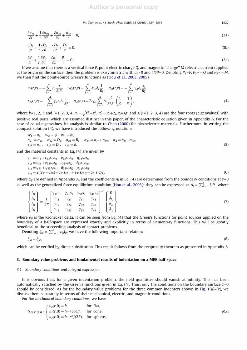
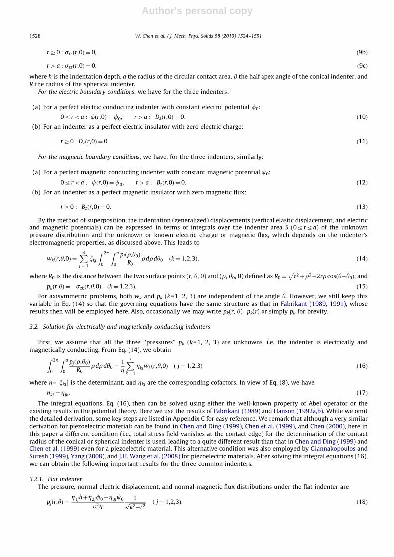
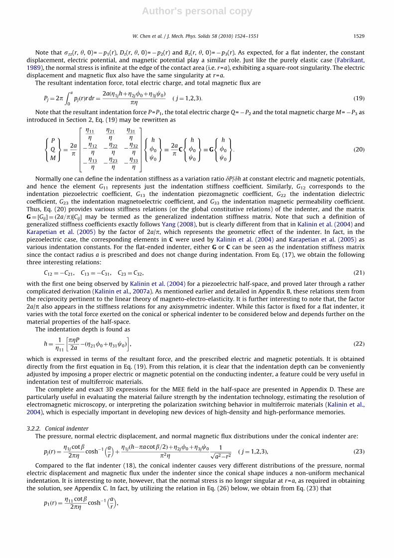


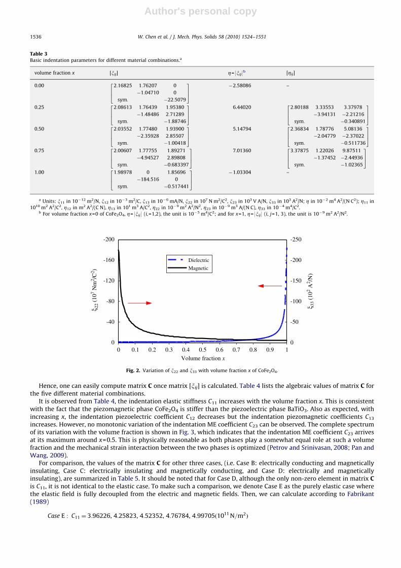


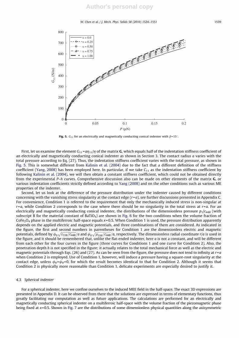


![Annual Report 2009-2010 rev[1] - University of Akronblogs.uakron.edu/otc/files/2014/02/Annual-Report-2009-2010_rev.pdf · Dr. Subramania Sritharan Professor, Water Resources Management](https://static.documents.pub/doc/80x56/5b7bef1d7f8b9a70138b9bfb/annual-report-2009-2010-rev1-university-of-dr-subramania-sritharan-professor.jpg)


