Author(s) Vladimir Novotny, Elias Manolakos, Timothy Ehlinger, Alena Bartošová, Neal O'Reilly, David Bedoya, Kevin McGarvey, Jessica Brooks, David Nathan Beach, Joseph Farah, and Richard Shaker is report is available at IRis: hp://iris.lib.neu.edu/ceus_pubs/2
Transcript
Author(s)Vladimir Novotny, Elias Manolakos, Timothy Ehlinger, Alena Bartošová, Neal O'Reilly, David Bedoya, KevinMcGarvey, Jessica Brooks, David Nathan Beach, Joseph Farah, and Richard Shaker
This report is available at IRis: http://iris.lib.neu.edu/ceus_pubs/2
MMooddiiffiiccaattiioonnss STAR Grant Agreement Number R83-0885-010
Vladimir Novotny (Primary Investigator) Elias Manolakos Timothy Ehlinger Alena Bartošová
Neal O’Reilly David Bedoya
Kevin McGarvey Jessica Brooks
David Beach Joseph Farah
Richard Shaker Submitted to the US Environmental Protection Agency
National Center for Environmental Research, Washington, DC
Iris Goodman, US EPA Project Director
Boston August 31, 2007
i
Acknowledgment and Disclaimer The research contained in this report was sponsored by the U.S. Environmental Protection Agency STAR Watershed Program by a Grant No. R83-0885-010 to Northeastern University. The authors greatly appreciate this support. The findings and conclusions contained in this report are those of the authors and not of the funding agency.
ii
Table of Contents
TABLE OF CONTENTS………………………………………………………………….ii EXECUTIVE SUMMARY………………………………………………………………..iv Objectives of the Research Projects………………………………………………………...iv Summary of Findings………………………………………………………………………. iv I. INTRODUCTION……………………………………………………………………… 1 Objectives………………………………………………………………………………….. 2 Project Activities…………………………………………………………………………… 3 The Team…………………………………………………………………………………... 6 II. DATABASE ACQUISITION AND DATA MANAGEMENT SYSTEM DEVELOPMENT………………………………………………………………………… 7 Database Structure…………………………………………………………………………. 7 Relational Databases………………………………………………………………………. 7 STAR Environmental Database……………………………………………………………. 7 Database Management and Implementation………………………………………………. 11 Data Sources and Availability……………………………………………………………... 12 Spatial Data – GIS…………………………………………………………………………. 13 III. DEVELOPMENT OF A MODEL FOR ESTIMATING NITROGEN FROM LAND USE AND OTHER MORPHOLOGICAL WATERSHED INFORMATION 15 Study Watershed Description……………………………………………………………… 15 Data Description………………………………………………………………………….... 16 Total Nitrogen Monitoring Data…………………………………………………………… 16 Watershed Characteristics and Nutrient Source Data ……………………………………... 17 Methodology / Principal Component Analysis……………………………………………. 17 Methodology / Components Regression…………………………………………………… 18 Results and Discussion / Principal Component Analysis………………………………….. 18 Results and Discussion / Components Regression Models………………………………... 19 Summary of Results and Conclusions……………………………………………………... 20 IV. FRAGMENTATION OF AGRICULTURAL LANDS AND IMPACT OF LAND USE TRANSFORMATION ON STREAM IBI IN SOUTH-EASTERN WISCONSIN……………………………………………………………………………… 23 Introduction………………………………………………………………………………… 23 Background………………………………………………………………………………… 24 Land Use, Watersheds and Biological Integrity…………………………………………… 24 Coupling Agricultural Landscape Metrics and Biotic Integrity…………………………… 25 Study Watershed Description……………………………………………………………… 26 Data………………………………………………………………………………………… 26 Fish Biological Data……………………………………………………………………….. 28 Methods / Calculation of Land Metrics……………………………………………………. 28
iii
Results……………………………………………………………………………………… 29 Stream Environmental Quality Model……………………………………………………... 29 Discussion………………………………………………………………………………….. 31 V. SSEELLFF –– OORRGGAANNIIZZIINNGG MMAAPPPPIINNGG OOFF DDAATTAA –– KKNNOOWWLLEEDDGGEE RREETTRRIIEEVVAALL FFRROOMM LLAARRGGEE DDAATTAABBAASSEESS…………………………………………………………………………………………………………………….... 3333 Introduction………………………………………………………………………………… 33 Self-Organizing Maps ……………………………………………………………………... 33 Ohio Datasets and IBI Fish Metrics………………………………………………………... 35 SOM Analysis for Maryland………………………………………………………………. 42 SOM Analysis for Wisconsin……………………………………………………………… 46 SOM Analysis for Minnesota……………………………………………………………… 49 Canonical Correspondence Analysis and Cluster Dominating Parameters………………... 49 Ohio Canonical Correspondence Analysis………………………………………………… 51 Maryland Canonical Correspondence Analysis……………………………………………. 53 Wisconsin………………………………………………………………………………….. 55 Impact of Variables on IBI Using k-means………………………………………………... 57 VI. DEVELOPMENT OF PREDICTIVE MODELS – HIERARCHICAL RISK PROPAGATION MODEL FOR INVERTEBRATES………………………………… 59 Study Area…………………………………………………………………………………. 59 Indirect Determination of Exposure Response Curve……………………………………... 59 Direct Effect of Environmental Variables…………………………………………………. 60 VII. PREDICTIVE MODELS DEVELOPMENT……………………………………… 63 Supervised ANN…………………………………………………………………………… 63 Methodology………………………………………………………………………………. 63 Developing Network Structure……………………………………………………………. 64 Selection of Environmental Input Parameters……………………………………………... 69 Predictive Models for Biotic Integrity Based on Variable Selection with Self-Organizing Maps (SOM), Polynomial Canonical Correspondence Analysis (PCCA) and Quadratic Regressions………………………………………………………………………………… 71 VIII. SYNTHESIS AND CONCLUSIONS……………………………………………... 77 General Findings…………………………………………………………………………… 77 SOM Findings ……………………………………………………………………………... 77 REFERENCES……………………………………………………………………………. 83 APPENDIX A – List of Technical Reports………………………………………………91 APPENDICES B-D Computer Models…………………………………………………..93
iv
v
EXECUTIVE SUMMARY Date of Report: August 20, 2007 EPA Agreement Number: R83-0885-010 Title: Developing of Risk Propagation Model for Estimating
Ecological Responses of Streams to Anthropogenic Watershed Stresses and Stream Modifications
Investigators: Vladimir Novotny, Timothy Ehlinger, Elias Manolakos, Alena Bartošová
Institutions: Northeastern University, Boston, MA (lead institution) University of Wisconsin, Milwaukee, WI, Illinois State Water Survey (University of Illinois), Champaign, IL
EPA Project Officer: Iris Goodman, Bernice Smith Research Category: Developing Regional-Scale Stressor-Response Models for
Use in Environmental Decision-Making, Water and Watersheds
Project Period: May 1, 2003 – May 31, 2007 Total Funds for the Project: $747,759
Objectives of the Research Project The goal of this research is the development of regionalized watershed-scale models to determine aquatic ecosystem vulnerability to anthropogenic watershed changes, pollutant loads and stream modifications (such as impoundments and riverine navigation). The models will assist watershed managers in their decisions on methods to mitigate stream degradation and biological impairment, assess potential watershed impacts, and identify watershed restoration opportunities. The layered hierarchical model system, developed by Artificial Neural Net (ANN) modeling and analysis, will be based on probabilistic risk propagation and linking the stresses with ecologic endpoints, from physical attributes of the watershed and water body and pollutant loadings at the lowest level to measures of biotic integrity, such as the Index of Biotic Integrity (IBI), at the highest level. The main objectives and outcomes of the research are: (1) Developing a model that would consider pollutant effects of impoundments for navigation and other purposes, channelization, watershed modification, and riparian corridor and land use changes as the key root stressors, using primarily data obtained from midwest streams; (2) Developing layered hierarchical progression of risks from basic root stressors to biotic endpoints (fish and macroinvertebrate IBIs); (3) Using the model to study the possibility of mitigating the stressors in a way that would have the most beneficial impact on biotic endpoints; (4) Developing a manual for watershed managers and other users; and (5) Investigating adaptability and transferability of the model to a stressed New England stream.
Summary of Findings Brief Description of the Project Tasks and Findings The first and very important step of the research was to acquire databases from several states and develop a data management system, which is described in Technical Report #5. Upon
vi
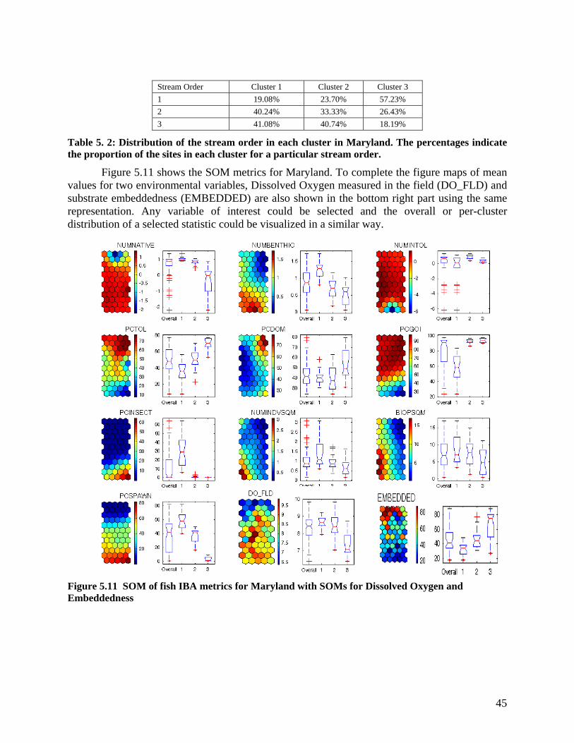
receiving the databases from Ohio and Maryland, we realized the biotic data were not taken in the same spot (section) as the chemical data. Therefore, in one of our studies, described in Technical Report #2, we focused on development of a nonlinear Principal Component Analysis model from the data obtained in Ohio, Illinois and Wisconsin that would estimate mean, 99% percentile of the log normal distribution of the data at a station, standard deviation and coefficient of variation. The model accurately predicted these variability parameters derived from total nitrogen concentrations at numerous sites. It was found the statistical variables are also a function of the mean, therefore the prediction of the coefficient of variation (standard deviation/mean) was the most accurate. Also in the first phase of our research (first two years) we established and demonstrated that a particular ANN structure, the Self Organizing Map (SOM), can be used to pattern and profile the distribution of stressors in large stream ecosystems, and discriminate sampling sites according to multi-stressor impacts. SOM were used to analyze the biological integrity of streams in Ohio and Maryland. This type of ANN analysis is called unsupervised learning. Each database contained between 1500 and 2000 sites and each site had measurements of fish and macroinvertebrate counts that were then converted into metrics of the fish and macro- invertebrate indices of biotic integrity. In addition, habitat metrics and water quality parameter values were also included in the databases. Consequently, the number of parameters analyzed at each site was 50 and more. The SOM analysis first organized the sites into 40 to 60 ANN neurons. Each neuron contains sites that are similar to each other. The neurons can be further organized based on their similarity into clusters. Typically, three to five clusters have been identified. The clusters can be ranked from bad to fair to good or excellent. In the SOM, by k-mean analysis, we identified the means of each parameter, including Macroinvertebrate index metrics, and identified those parameters that exhibited similar distribution of neurons as the SOM for the fish metrics and those that did not. Then using Canonical Correspondence Analysis (CCA) and Principal Component Analysis (PCA), the research teams identified ranking of stressors as to their impact on IBI and Cluster Dominating Parameters (CDP). It was found the habitat parameters such as embeddedness, gradient, substrate, and riparian zone characteristics are the most important CDPs that impact the biotic integrity of streams. The SOM model and its application to Ohio and Maryland databases is described in Technical Report #4. In the second phase of the research (2004 –2007), SOM analysis was expanded to Minnesota (Technical Reports #12 and 13). Figure 1 shows the visual representation of the clusters for Ohio. The cluster dominating parameters identified by the Canonical Correspondence Analysis and their impact on IBI are shown on Figure 2. The SOM modeling software and manual is a public domain product of our research. It was found that in Ohio’s Cluster III contained mostly impounded (channelized) stream reaches. The analysis of data showed a relatively higher correlation between habitat parameters (channel, embeddedness, pool, substrate, riffle and cover) and the fish IBI, which was better than that between the other environmental variables (chemical and land uses) and IBI. In Maryland, from the full set of variables, after removing the qualitative variables and subgrouped variables (such as high urban and low urban), 38 environmental variables were correlated with IBI. Three clusters based on geographical grouping provided distinctive correla- tion matrices and principal components. The first two principal components for Cluster 1 (coastal plains) showed high forest land use and urban loadings as most dominant. Similarly, Cluster 2 (Appalachian Plateau) showed high forest and agricultural loadings, and Cluster 3 (Piedomont) showed high urban and agricultural loadings and correlations with IBI (R2~0.5).
vii
Figure 1 Results of the SOM analysis for Ohio data showing organizing of metrics in neurons. Three clusters were identified and the ranges of IBIs in the clusters are shown.
Figure 2 Canonical Correspondence Analysis identified the Cluster Dominating Parameters, their degree of cross-correlation and magnitude of the impact.
In the second phase of the research (third and fourth year), we capitalized on the very promising results of the first phase. We added supervised ANN based prediction capabilities as a step following the hierarchical unsupervised nonlinear clustering of sampling sites according to fish IBI metrics distribution. In the supervised ANN modeling (Technical Report #3) we linked fish IBI as an dependent variable by back propagation ANN with all the inputs. Extensive effort was made not to overtrain the ANN model.
One of the most important outcomes of our research is the finding that IBI can be better predicted with actual measured habitat parameters than using their scores. Typically scores are assigned as integer values e.g., 1, 3, 5 where 1 is the low score and 5 is the high score. This is a very coarse quantification of a variable. The effect on prediction is shown on Figure 3 ab.
This finding led to a recommendation for development of better IBI predicting models. It should also be pointed out that not all habitat metrics and other measured environmental variables (land use, habitat, and water quality) are relevant for predicting IBIs, which is described in the reports. Also not all fish metrics show SOM distribution over the clusters.
viii
Figure 3 Comparison of predictive capability of IBI models. Left using habitat scores of the metrics
and right using measured values of the metrics.
The University of Wisconsin (Milwaukee) team, using an extensive fish, habitat and land cover database for the State of Wisconsin, has developed a GIS based system to be used for analyzing impacts of stream habitat and fragmentation, hydrological and hydraulic parameters, and watershed land use on the stream biological integrity (Technical Report # 11).
Risk Propagation model for IBI of benthic invertebrates (Tech. Report # 9). This analysis and model development was conducted by the Illinois State Water Survey.
Two biotic indexes using information on macroinvertebrate communities were calculated: Macroinvertebrate Biotic Index (MBI) used in Illinois and Invertebrate Community Index (ICI) developed in Ohio. MBI represents a tolerance index and ICI represents a multi-metric index. The variability in biotic indexes due to environmental variables was quantified using multiple regression analysis with backward selection. The impacts of both the direct effect variables (e.g., concentrations of contaminants) and indirect effect variables on these indices were investigated. In northeastern Illinois, the direct effect of environmental variables results in stronger multiple regression equations, explaining the higher percentage of variability in data than when using risk variables. In all cases, up to 55% variability was explained by the model. Although a large portion of variability remains unexplained, all relationships are statistically significant and stronger than typically reported in the literature.
Conclusions SOM analysis and knowledge data mining is a powerful tool that can identify similarities between multiple dimensional vectors of IBI metrics as dependent variables and habitat metrics, invertebrate indices, serving in this project also as surrogates for sediment contamination, land use and riparian zone characteristics, and water quality parameters. Clustering of the sites and determination of the Cluster Dominating Parameters by the SOM and follow up Canonical Correspondence Analysis (linear or nonlinear) provides then useful predictive models. However, these models typically can explain 50 or slightly more of the variability of the total IBI and its metrics. Several types of predictive models have been and can be developed: (1) SOM only
ix
models where the unmonitored sites are matched with the neuron in the SOM that contains the sites of the closest similarity with the unmonitored site. Then the mean IBI in the neuron would represent the prediction; (2) supervised back propagation – feed forward ANN models; and (3) nonlinear Canonical Correspondence (PCCA), Multiple Range Test (MRT) or Principal Component Analysis (PCA) advanced statistical models. The last category of models enables identification of the qualitative impact of the Cluster Dominating Parameters. Presentations/Publications
Over the four year period the research project produced 12 technical reports derived from work of the primary investigator and from the theses and other work by the MSc and PhD level research associates. These technical reports will be made available from the Northeastern University Library and published on the web site of the Center for Urban Environmental Studies of the Northeastern University in Boston (http://www.coe.neu.edu/environment). The following is a list of professional publications and presentations as of August 2007. After the conclusion of the project, the team will prepare and submit several other publications to peer review journals. Selected publications derived from the research: V. Novotny, A. Bartošová, N. O’Reilly, and T. Ehlinger (2005) Unlocking the Relationships of
Biotic Integrity to Anthropogenic Stresses, Water Research 39(1):184-198 V. Novotny (2003) Key Note Lecture - The next step - incorporating diffuse pollution abatement
into watershed management, Proceedings of the 7th International Specialized Conference on Diffuse Pollution and Basin Management - DipCon, International Water Association, Dublin, Ireland, August 17-22, 2003, Water Science & Technology
V. Novotny (2004) Watershed Vulnerability Assessment - a Tool of Watershed Management, Milan Straskraba Memorial Lecture, Czech Academy of Science and University of Southern Bohemia in Ceske Budejovice, June 24, 2004
D.N. Beach and V. Novotny (2005) Modeling In-Stream Nitrogen Concentrations Based on Drainage Area Characteristics and Principal Components Analysis, Proc. AWRA National Conference, Seattle, WA, November, submitted to Journal AWRA, revised and resubmitted (2007)
V. Novotny (2006) Agricultural diffuse pollution: Are we on the right track to successful abatement? Invited Key Note Presentation, Proc. SEPA/SAC Biennial Conference – Agriculture and the Environment – Managing Rural Diffuse Pollution, April 5-6 2006, Edinburgh, Scotland
V. Novotny and E. Manolakos (2006) Ecological clustering of integrity and nonlinear impact of environmental variables, Invited Keynote presentation, Proc. RESLIM 2006 International Conference, August 27 – September 1, Brno, Czech Republic
E. Manolakos, H. Virani, and V. Novotny, Extracting Knowledge on the Links between the Water Body Stressors and Biotic Integrity, Water Research, accepted for publication 2007
K. McGarvey and V. Novotny (2007) Evaluation of Impact of Land Use, Habitat, and Water Quality Parameters on Macroinvertebrate Index Metrics by Redundancy Polynomial Regression Analysis, Proc. Massachusetts Water Resources Conference, Amherst, Ma, April
D. Bedoya and V. Novotny (2007) Quadratic Multivariate Regression and Self-Organizing Maps (SOM) for Fish Metrics Prediction in Ohio, Proc. EWRI´s World Environmental & Water Resources Congress, Tampa, FL (2007)
1
I. INTRODUCTION11 Among the list of global environmental problems, no single item holds greater
consequence for the human condition than the problems associated with the distribution, abundance, and quality of fresh water. The creation of legislation and the implementation of policies directed toward stopping and reversing the degradation of water resources are critically important and significant progress has been made in developing technologies and strategies for managing anthropogenic stressors originating from identifiable point sources of pollution. However, analysis of data collected from monitoring studies conducted by state pollution control agencies over the past decade show the control of point source pollution alone is seldom sufficient to restore ecological structure and function to degraded rivers and streams (Allan, 2004). This resulted in an increased focus on understanding larger scale watershed processes and land use patterns, and led to a greater emphasis on controlling the accumulated impact of diffuse, non-point source pollution on aquatic ecosystems (Allan, 2004).
Although it is both attractive and necessary to adopt a watershed perspective in order to address water resource degradation and recovery, the larger spatial and temporal scale present a complex suite of problems for monitoring, identification of stressors, and the implementation of management strategies. The United States Clean Water Act set forth the national goal of “restoring and maintaining the chemical, physical and biological integrity of the Nation’s waters”. Integrity was defined as a condition of a water body to support a balanced aquatic life resembling as close as possible the natural state. The concept of an “Index of Biological Integrity” (IBI) was developed and published by Karr et al (1986) and follow up publications, for example, Karr (1991), as a method to quantify the ecological impact of human-induced alterations in stream ecosystems using fish and macroinvertebrate organisms as indicators. An IBI is constructed from field-measured component metrics that include parameters related to species richness and composition, trophic composition, and organism abundance and condition, and is based upon the premise that fish respond to environmental stressors in a species- or guild-specific manner. The IBI metrics and guidelines were published by Karr and co-workers and finally incorporated into the US EPA guidance document (Barbour et al., 1999). However, many states use their own modifications of the metrics. IBI is then a summation of the values ascertained for each metric. Metrics are scaled relative to covariation with natural factors (e.g. stream size or geographical distinctions), and when properly calibrated, allow for the calculation of a “rating” that describes the streams ecological health relative to best case, or non-impacted ecoregional reference. Thus IBIs can provide a “biological response signature” for monitoring compliance with antipollution regulations (Yoder and Rankin, 1999; 1998).
Watershed managers need to be able to make an assessment of multiple stressor effects on ecological vulnerability of the water bodies, point out those stresses that have the largest impact and, subsequently, propose and develop a cost-effective remediation strategy. Biotic monitoring programs have increased steadily, and researchers are asking whether IBI-related data can be used within a watershed-based restoration/management context to help identify the relative severity of individual stressors that are responsible for causing degradation and/or preventing recovery (Yuan and Norton, 2003). The benefits of being able to do this are far
1 See Technical Report # 1 for details.
2
reaching, not the least of which include being able to direct limited financial resources more efficiently to monitoring and remediation activities.
The traditional, single number IBI is not well-suited for this type of analysis because its premises and construction mask the nonlinearities, covariation, and spatial scale variation that are inherent in the stressor-response relationships (Niemi et al., 2004). The general idea is that by studying the responses of individual metrics from which IBIs are derived, there is greater power to be able to detect and characterize the functional linkages between stressors and responses. In order to do this, methodologies for analysis and interpretation are required that can examine the responses of individual guilds, traits, and species, and then connect the mechanistic “chain of influence” from anthropogenic activities (e.g. land use) to biological responses in streams. The progression of the effects of stressors from landscape to instream impacts (chemical and habitat risks) to the biotic endpoints (fish and macroinvertebrate IBIs and their metrics) is hierarchical and layered (Novotny et al., 2005) and shown on Figure 1.1.
Objectives The goal of the research was the development of a regionalized watershed-scale model to determine aquatic ecosystem vulnerability to anthropogenic watershed changes, pollutant loads and stream modifications (such as impoundments and riverine navigation). The main objectives and outcomes of the research were:
(1) Developing a model that would consider effects of impoundments for navigation and other purposes, channelization, watershed modification, and riparian corridor and land use changes as the key root stressors, using primarily data obtained from the midwest
Landscape morpho-logical/ riparianfactors and stresses
ECOREGION
Land use changefactors and stresses,imperviousness
Pollutant loads fromland, point sourcesand atmosphere
Hydrologic/hydraulicstresses
LAYER 4
Periphyton and its metrics
BIOTICENDPOINTS
RISKS
IN-STREAM STRESSES
LANDSCAPE/ATMOSPHERIC STRESSES Figure 2 Hierarchical layered links of watershed and in-stream stressors to the multimetric biotic indices (from Novotny et al., 2005)
3
streams; (2) Developing layered hierarchical progression of risks from the basic root stressors to the biotic endpoints (fish and macroinvertebrate IBIs); (3) Using the model to study the possibility of mitigating the stressors in a way that would have the most beneficial impact on the biotic endpoints; (4) Investigating adaptability and transferability of the model to a stressed New England stream; and (5) Advise managers on the use of the model in their assessment of integrity, identification of causes of degradation and developing remedial measures.
Project activities • Forming the team
Teams have been established at Northeastern University (lead institution) and University of Wisconsin – Milwaukee (subcontractor). In addition, services of Dr. Alena Bartošová from the Illinois State Water Survey were also subcontracted.
• Conducting literature review An extensive literature review has been prepared by the Primary Investigator (Technical Report # 1) that was subsequently published in a peer reviewed journal article.
• Acquiring the data Large databases were obtained from
o State of Ohio (from Ed Rankin of the Midwest Biodiversity institute at Ohio University)
o State of Maryland o State of Massachusetts o State of Minnesota o State of Wisconsin
Smaller data sets were retrieved for selected rivers in Ohio (Maumee River) and Illinois (Fox River). The data were organized and entered into the databases.
• Developing Database Management software. STAR Environmental Database (STARED) was developed by the Illinois State Water Survey and put on a dedicated computer server located at and operated by the Northeastern University (see Technical Report # 5).
• Development of a Principal Component Analysis (PCA) model for estimating nitrogen (and also other water quality parameters) from land use and other morphological watershed information. Often, the location of collected biotic information does not coincide with the location of the water quality monitoring stations. To estimate key the mean and extremes (variability) of key water quality parameters, a PCA models were developed for streams in Ohio and also tested on the Fox River in Illinois. The model estimate means, standard deviations, 99 percentile (non exceedance) concentrations, and coefficient of variation for nitrogen. The best correlation was received for the coefficient of variation (Technical Report # 4 plus a publication).
• Fragmentation of agricultural lands and impact of land use transformation on streams in southeastern Wisconsin. This research at the University of Wisconsin – Milwaukee examined the effect of transition of the landscape of exurbia and its effect on integrity of streams. 31 watersheds were used to separate southeastern Wisconsin into analyzable landscapes. The overall objectives were: (1) to identify a subset of metrics
4
that capture the majority of variation in agriculture land fragmentation in southeastern Wisconsin, and (2) to identify a subset of metrics that capture the relationship between agricultural land fragmentation and a measure of biotic integrity (IBI: an index score based on fish population variables). Seventy-two landscape metrics were calculated and statistically analyzed. In the end, six landscape metrics were identified that explained 84% of the variation in the aquatic environmental integrity for southeastern Wisconsin. The strength of these relationships indicates that the spatial design of human development in watersheds has a significant impact on aquatic ecological integrity and principles of landscape design may have direct relevance to efforts of river and stream restoration and protection.
• Development and application of Self Organizing Mapping to sort and analyze the large data matrices Kohonen’s Self Organizing Mapping (SOM) software model based on unsupervised Artificial Neural Networks (ANN) was developed using MATLAB modeling package. The SOM is one of the most popular neural network structures based on competitive learning. It consists of the input (data) layer and the output (map) layer. Each neuron of the input layer represents an input variable and has a weighted connection to each node of the output layer. The connection weights are adaptively changing at each iteration of an unsupervised training algorithm. The algorithm implements a nonlinear projection from the high-dimensional input space onto a low-dimensional network of neurons (usually a 2-dimensional grid) in an orderly manner. This is achieved by unsupervised training, which means that no “teaching output” is needed during the learning process. SOMs have a great utility when dealing with large multimetrics databases. SM nalyses were performed using databases obtained from the Ohio EPA, Maryland Biological Stream Survey (MBSS), Wisconsin DNR, and Minnesota Pollution Control Agency (MNPCA). The details and the results have been described in the Technical Report # 4 and in an abbreviated form in Chapter 5 of this final report.
• Supervised Artificial Neural Network and Linear and Nonlinear Canonical Correspondence Analysis modeling. These efforts were looking for the nonlinear relationships between the stressors at various levels of hierarchy and endpoints that were the overall IBIs or their individual metrics. The models were developed for the entire state or, after preprocessing by SOM, separately for the clusters. Both ANN and CCA regressions performed well and could account for 50% or more of the variability. Efforts have been made to make the model parsimonious by eliminating parameters that were cross-correlated (as determined by the SOM analysis). It was possible to reduce the number of input parameters from about 35 to 15 or less without reducing significantly the predictive capability of the models.
• Development and testing predictive model based on risk propagation concept for benthic macroinvertebrates in Illinois and Wisconsin. The risk propagation model is a probabilistic progression of stresses as outlined on Figure 1.1. The macroinvertebrate IBI was then correlated to the calculated risks imposed by various stressors.
• Development and testing predictive models based on Principal Component Analysis for benthic macroinvertebrates for Massachusetts. The Massachusetts database was small and incomplete and did not allow a full SOM and ANN analyses. Therefore, logarithmically transformed values of the measured macroinvertebrate indices were
5
correlated by Principal Component Analysis to the measured stressors available from the database. This effort described in Technical Report # 15.
• Synthesis and development of methodologies based on the results of the research. The research has found that approximately one half of measured parameters do not contribute to the variability of the indices. Furthermore, some metrics also have less relevance in some states and, also, stresses expressed by ranking of habitat metrics were less explanatory than the actual measured parameters. This gives an impetus for reevaluation of the structure of the IBIs, including the clustering concepts (that to some degree correlate well with geographical ecoregions in some states) and suggesting reformulating the inputs of the models.
Figure 1.2 shows the states and watersheds included and analyzed this research for which the models were developed. The technical reports developed in this research are listed in the reference section of this final report.
IL
MN
WI
OH
MD
MA
States With Data in this Project±
0 240 480 720 960120Kilometers
Fox River Watershed
Great and Little Miami Rivers Watershed
Figure 1.2 States and watersheds in the study
6
The Team The team was headed by the Primary Investigator, Dr. Vladimir Novotny, CDM Chair at Northeastern University, and included investigators from three universities. The following researchers and graduate students participated on the project: Northeastern University
Professor Vladimir Novotny (Primary Investigator), Department of Civil and Environmental Engineering Professor Elias Manolakos, Department of Electrical and Computer Engineering (2003-2005)
Dr. Ramanitharan Kandiah (postdoctoral fellow), Department of Civil and Environmental Engineering and Center for the Urban Environmental Studies (2004-2006)
Dr. Laurel Schaider (postdoctoral fellow), Department of Civil and Environmental Engineering and Center for Urban Environmental Studies (2004)
Graduate Students: David Nathan Beach (CEE), Jessica Brooks (CEE), and Hardik
Virani (ECE) (2003 to 2005). All three completed MSc thesis that were converted to technical Reports (see list below).
Kevin McGarvey (MSc) and David Bedoya (PhD) (2005-2007). Kevin Mc Garvey completed MSc thesis converted into a technical report. David Bedoya authored two technical reports. His thesis developed from this research will be completed in 2008. Joseph Farah (MSc student) joined the team in 2006 and participated on several technical reports.
University of Wisconsin – Milwaukee Professor Timothy Ehlinger, Department of Biological Science, Director, Conservation
and Environmental Sciences Program Graduate Students: Neal O’Reilly (2004-2007), Dwight Osmon (2003-2004), Kathleen
Hoverman (2005), and Richard Shaker. Kathleen Hoverman and Kevin Shaker prepared technical reports, Neal O’Reilly (2005-2007) of Hey and Associates was a graduate student at Marquette University who worked on his PhD research with the UWM team. He submitted a technical report derived from his PhD thesis and will graduate in 2007.
Illinois State Water Survey (University of Illinois) Champaign-Urbana Dr. Alena Bartošová developed the database management system and the risk propagation model for invertebrates in the Illinois Fox River.
7
II. DATABASE ACQUISITION AND DATA MANAGEMENT SYSTEM DEVELOPMENT2
Database Structure
Environmental data needed for the study are acquired from different sources and consequently in different formats. Illinois State Water Survey (ISWS) faced a similar problem when compiling data for the Fox River Watershed Investigation (McConkey et al. 2004). The Fox River (tributary to Illinois River) is one of the watersheds selected for this study. The relational database FoxDB created by the ISWS served as an excellent starting point when developing a database structure for this project and populating it with data.
Relational Databases A database was constructed with the data structures such as data objects, the governing
rules, and associations related to the data objects based on a concept, a data model. A data model is specific to the horganization of the data instead of the type of operations to be executed or hardware and software used. In this way, a data model correlates the concepts that make up real-world events and processes, with the physical representation of those concepts, in a database. In addition to being relatively easy to create and access, a relational database has the important advantage of being easy to extend. After the original database creation, a new data category can be added without requiring that all existing applications be modified.
A relational database is a set of tables containing data in predefined categories. Each table contains one or more data categories in columns. Each row contains a unique instance of data for the categories defined by the columns. The tables are then related back to each other by the database engine when requested. A database user can obtain a view of the database that fits the user's needs. While creating a relational database, one can define a domain of possible values in a data column and further constraints that may apply to that data value. The standard user and application program interface to a relational database is the structured query language (SQL). SQL statements are used both for interactive queries to retrieve data and for displaying data in reports.
Tables include a unique identifier for each instance. This unique identifier can be used in other tables to refer to the particular instance without repeating all the information about that instance again, thus providing necessary links among related tables. The process of removing redundant data from a relational database by separating information into smaller tables is called normalization. A normalized database is a database with relations that follow a series of rigorous standards. It generally improves performance, lowers storage requirements, and makes it easier to change the application or to add new features. STAR Environmental Database (STARED) A comprehensive database, STAR Environmental Database (STARED) was developed to store various environmental data, including water quality, sediment chemistry, biological indices, stream hydrology, and habitat. The structure is based on a structure of the FoxDB, the relational 2 See technical Report # 5 for details
8
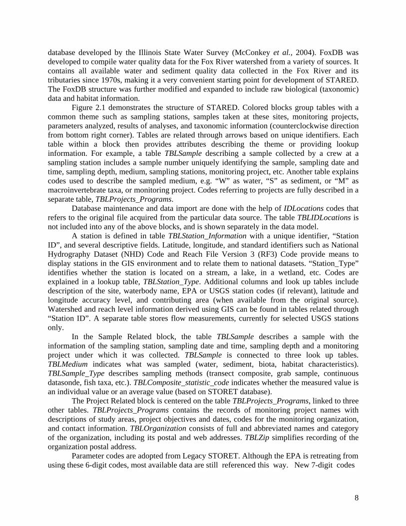
database developed by the Illinois State Water Survey (McConkey et al., 2004). FoxDB was developed to compile water quality data for the Fox River watershed from a variety of sources. It contains all available water and sediment quality data collected in the Fox River and its tributaries since 1970s, making it a very convenient starting point for development of STARED. The FoxDB structure was further modified and expanded to include raw biological (taxonomic) data and habitat information. Figure 2.1 demonstrates the structure of STARED. Colored blocks group tables with a common theme such as sampling stations, samples taken at these sites, monitoring projects, parameters analyzed, results of analyses, and taxonomic information (counterclockwise direction from bottom right corner). Tables are related through arrows based on unique identifiers. Each table within a block then provides attributes describing the theme or providing lookup information. For example, a table TBLSample describing a sample collected by a crew at a sampling station includes a sample number uniquely identifying the sample, sampling date and time, sampling depth, medium, sampling stations, monitoring project, etc. Another table explains codes used to describe the sampled medium, e.g. “W” as water, “S” as sediment, or “M” as macroinvertebrate taxa, or monitoring project. Codes referring to projects are fully described in a separate table, TBLProjects_Programs.
Database maintenance and data import are done with the help of IDLocations codes that refers to the original file acquired from the particular data source. The table TBLIDLocations is not included into any of the above blocks, and is shown separately in the data model.
A station is defined in table TBLStation_Information with a unique identifier, “Station ID”, and several descriptive fields. Latitude, longitude, and standard identifiers such as National Hydrography Dataset (NHD) Code and Reach File Version 3 (RF3) Code provide means to display stations in the GIS environment and to relate them to national datasets. “Station_Type” identifies whether the station is located on a stream, a lake, in a wetland, etc. Codes are explained in a lookup table, TBLStation_Type. Additional columns and look up tables include description of the site, waterbody name, EPA or USGS station codes (if relevant), latitude and longitude accuracy level, and contributing area (when available from the original source). Watershed and reach level information derived using GIS can be found in tables related through “Station ID”. A separate table stores flow measurements, currently for selected USGS stations only.
In the Sample Related block, the table TBLSample describes a sample with the information of the sampling station, sampling date and time, sampling depth and a monitoring project under which it was collected. TBLSample is connected to three look up tables. TBLMedium indicates what was sampled (water, sediment, biota, habitat characteristics). TBLSample_Type describes sampling methods (transect composite, grab sample, continuous datasonde, fish taxa, etc.). TBLComposite_statistic_code indicates whether the measured value is an individual value or an average value (based on STORET database). The Project Related block is centered on the table TBLProjects_Programs, linked to three other tables. TBLProjects_Programs contains the records of monitoring project names with descriptions of study areas, project objectives and dates, codes for the monitoring organization, and contact information. TBLOrganization consists of full and abbreviated names and category of the organization, including its postal and web addresses. TBLZip simplifies recording of the organization postal address.
Parameter codes are adopted from Legacy STORET. Although the EPA is retreating from using these 6-digit codes, most available data are still referenced this way. New 7-digit codes
were created specifically in this project for habitat parameters or biological indices not included in the original STORET codes but needed for the analyses. The table TBLParameter_Codes in the block Parameter Related closely follows the parameter table from Legacy STORET with full and abbreviated description of parameters, reporting unit, and accuracy. Look up information is provided in the following tables: TBLReporting_Units, TBLGroup_Code, TBLMedia_Group, TBLParameter_Group, TBLGroup_Codes, and TBLQAPP_Groups.
For grouping parameters, two schemes, Legacy STORET scheme and QAPP scheme are used in this database. The QAPP scheme was developed by the ISWS (McConkey et al. 2004) together with the QAPP grading system to allow evaluation of data quality. The QAPP scheme groups parameters on two levels, by sampled medium, and by constituent analyzed. The three-digit coding scheme of QAPP enables to identify the medium, the main parameter group and the constituent subgroup. The main parameter group includes basic inorganic, nutrients, metals and organics; and the constituent subgroup comprises of a number of groups such as nitrogen in the nutrients group or pesticides in the organics group.
The Taxa Related block provides taxonomic information on aquatic biota, presently fish and macroinvertebrates although the structure enables incorporating other taxonomic groups such as algae or macrophytes. The USDA houses the Integrated Taxonomic Information System (IT IS) database developed to provide accurate, scientifically credible, and current taxonomic data and to serve as a standard to enable the comparison of biodiversity datasets (USDA, 2004). The IT IS taxonomic classification and codes were adopted into the STARED. The IT IS code is similar to the STORET parameter codes -- it basically describes what can be found or analyzed in a sample. The taxonomic part of the table TBLITIS_Code mimics the IT IS structure defining taxonomic hierarchy with Latin and common names, parent taxa, and taxonomic rank. Other information relating specifically to this project includes the assessment group (fish or macroinvertebrates), and a code specifying whether the species is native. The table TBLIndices_Group assigns species or taxa to the most common groups used in deriving the index of biotic integrity, such as Amphipods or Chironomids for macroinvertebrate indexes and darters or simple lithophilic spawners for fish indexes. Indices also include feeding preferences of the taxa, e.g., collectors, gatherers, herbivores, or insectivores.
Results described in the Results Block define actual values of parameters analyzed in a sample. Numerical and non-numerical results are stored in separate tables, TBLResults and TBLResults_Vol_NonNumeric, respectively. The third table, TBLReplicates is used to store all replicate results. Biological ‘catch’ data are stored in the table TBLBio_Taxa. The structure of these tables is very similar. For each sample identified by a unique ID, the result is the concentration value for a parameter specified by the Parameter Code, or number of individuals for a species defined by the IT IS Code, respectively. A remark code may accompany a result with additional information about the quality issues such as “below the detection limits” or “calculated value”. Unreliable or questionable data may be indicated with an optional grade and comment.
The complete data dictionary with description of the tables and fields is given in Appendix of the Technical Report # 5.
. Database Management and Implementation
The master database was stored in Microsoft SQL Server 2000 format on a server connected to a network. This setup allows multiple users to access the data either directly using
11
SQL Server or the Open Database Connectivity (ODBC) interface. The database is managed by Northeastern University. The ODBC interface allows data accessing among various software applications regardless of vendor. For example, the user can link Microsoft Access to tables stored in Microsoft SQL Server and access the data in real time. Tables and queries created in Access or SQL Server can also be easily imported to Excel, ArcGIS or other software for display and analysis.
A Two-level access database architecture is recommended. All users can access the database through a client connection and query the database to extract desired information. Individual users do not need their personal copy of the database as they are connected via the network to the master copy. Considering the data security, only the database manager has full access to the database, can add and delete data, and modify the database structure. All other users can forward any relevant and preformatted data to the database manager for import. Their privileges are specified as read-only.
DatabaseServer
Database Manager
Data Source
Data Source
Data Source
User User
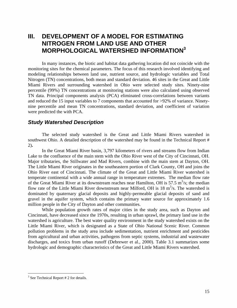
Figure 2.2 Database architecture, showing multiple users connected to a single database server. The master copy of the database, STARED is currently stored on SQL Server, SPRUCE18 at Northeastern University, Boston. The data manager operates from the Center for Urban and Environmental Studies at Northeastern University to update the database structure, to coordinate data import, to provide necessary quality control, and to ensure database integrity. The personnel in the Information System/System Administration Department of the Northeastern University are responsible for the maintenance of the server. Users from both within and outside the NEU network can access the database. Data acquired and preformatted by the project team are forwarded to the data manager for final quality check and import. Any documentation aiding in interpreting the data beyond the information stored in STARED is saved on SPRUCE18 in a separate folder.
Data Sources and Availability
The developed database is targeted to contain data from a variety of sources. Data acquired by the ISWS in the FoxDB (McConkey et al. 2004) represent an integral part of STARED. Additional data were acquired from major federal and state agencies collecting data in the study area.
12
These agencies include the US Environmental Protection Agency (USEPA), Ohio Environmental Protection Agency (OEPA), Illinois Department of Natural Resources (Illinois DNR), Illinois Environmental Protection Agency (IEPA), Maryland Department of Natural Resources (Maryland DNR), US Geological Survey (USGS), Minnesota Pollution Control Agency (MPCA) and the Massachusetts Department of Environmental Protection (MADEP). Additional data were retrieved from federal sources from the USEPA STOrage and RETrieval (STORET) System, the USGS National Water-Quality Assessment (NAWQA) Program, and the USGS National Water Information System (NWIS) which are major federal databases of environmental data available on the internet. The Fox River Watershed Water Quality Database (FoxDB)
The FoxDB is a prototype for the database as well as a source of data for the development of the Risk Propagation Model (see Chapter 6). The database was developed by the Illinois State Water Survey. All available data on water quality (water and sediment chemistry data) and other related parameters that define the nature of the stream and river environment were compiled into one database. Stream flow data are included as an integral part to interpret reported concentrations of chemical water constituents. This database has been designed so that it can be expanded in the future to include other types of data and data from other watersheds (McConkey et al., 2004). Maryland Biological Stream Survey (MBSS) Data
The Maryland Biological Stream Survey data included 955 first, second and third-order stream segments, encompassing all 17 major drainage basins in the state of Maryland over the three-year sampling period (1995-1997). Statewide and basinwide results and an assessment of the condition of the streams were reported in the MBSS three-year report (Roth et al., 1999). Water chemistry and benthic macroinvertebrates were analyzed in spring (March-April) while fish, physical habitat, and in-situ water chemistry were analyzed in summer (June-September). All sampling sites are classified into three geographic regions: west, central, and east. Biological measurements include abundance and health of fish, composition of benthic macroinvertebrate communities, and presence of amphibians and reptiles, aquatic plants, and mussels. Chemical measurements include pH, sulfate, nitrate-nitrogen, conductivity, and dissolved oxygen. Physical habitat measurements took into account parameters such as flow, stream gradient, maximum depth, embeddedness, instream habitat, epifaunal substrate, pool and riffle quality, bank stability, channel flow status, shading, and riparian buffer type (Mercurio et al., 1999). Ohio EPA Data
The Ohio dataset was assembled from the chemical, habitat and biological data collected by the Ohio EPA since 1967. However, the data available for the period before 1990 are few in numbers. The chemical data are available for water, sediment, and fish tissue. The original data set is available in the FoxPro format. The fish tissue database currently holds 5,058 samples collected from 1967 through 1996. The fish tissue was analyzed for pesticides and PCBs (3,978 samples), metals (2,865 samples), VOCs (57 samples), BNAs (166 samples) and herbicides (44 samples). The database was provided by Ed Rankin of the Institute for Local Government Administration and Rural Development (ILGARD) of the Ohio University and Midwest Biodiversity Institute in Athens, OH.
13
Minnesota Pollution Control Agency Data The Minnesota Pollution Control Agency (MPCA) biological data were acquired, and
reformatted to fit STARED structure (MPCA, 2005; Genet and Chirhart, 2004). This data set consists of data spread sheet for the whole state, and covers twenty year period data. Illinois EPA Data The Illinois EPA conducts a wide variety of water quality monitoring programs. Stations are sampled for biological, chemical and/or in-stream habitat data, as well as streamflow. A fixed network of stations is sampled on a 6-week sampling frequency with the samples analyzed for a minimum of 55 universal parameters, including field pH, temperature, specific conductance, dissolved oxygen (DO), suspended solids, nutrients, fecal coliform bacteria, and total and dissolved heavy metals (IEPA, 2005). The monitoring program also includes intensive stream surveys (incl. biological and habitat data) with all watersheds being sampled once in a 5-year rotation.
Water chemistry data for the Fox River watershed were already a part of the FoxDB. Biological and habitat data were acquired from the Illinois EPA and imported into STARED.
Massachusetts Data A database was obtained from the Massachusetts Department of Environmental Protection (MA-DEP), Division of Watershed Management that contained macroinvertebrate metrics of biological integrity and associated quantitative physical habitat for each location. Massachusetts does not have a macroinvertebrate index of biological integrity but uses other metrics described in the Rapid Bioassessment Protocol (Barbour et al., 1999). One of the metrics Massachusetts uses is a modification of the Hilsenhoff Biotic Index.
Spatial Data – GIS Spatial data is formatted to be displayed and analyzed in Geographic Information System
software. Examples of spatial data formats include: digital elevation models (DEM) stored as raster data, ArcGIS layer files (or ArcView shapefiles) representing monitoring point locations, land use, ecoregions, and soil type, and hydrography files describing the shape and spatial properties of streams. Many federal and state agencies operate and maintain databases of spatial information, including downloadable data for use in GIS software.
The National Hydrography Dataset (NHD) is developed on Digital Line Graph (DLG) of USGS integrating the Reach File Version 3 (RF3) of USEPA to provide information on waterbodies such as rivers, ponds, streams and lakes. The NHD supersedes RF3 and DLG datasets. The NHD can be downloaded in three different resolutions, high, medium and local. Medium resolution (1:100000) is available for the conterminous states area. High (1:24000) or local (varies) resolution hydrography is being developed and its availability varies among the states and watersheds. The full description of the NHD data as well as a download tool can be found at http://nhd.usgs.gov/.
The NRCS provides 1:250,000 scale digital soil information from the State Soil Geographic Database (STATSGO). This digital geographic data is available in several formats including: digital line graph files and ARC/INFO coverages. The STATSGO includes information about the location of soil types and are linked to the Soil Interpretations Record (SIR) attribute database. The SIR includes information about soils’ respective properties,
14
including 25 physical and chemical properties. Higher resolution data (SSURGO) may be available on a county level.
The most current information on land use can be found on a state level. Statewide GIS coverages on Illinois state land use information can be obtained from the Illinois Department of Agriculture. The Illinois Interagency Landscape Classification Project (IILCP) produced coverage detailing land use in 1999–2000. The primary source for this digital information was LANDSAT satellite imagery from three different seasons and is classified by 23 different land use categories. Wisconsin state land use information can be obtained from the Wisconsin Department of Natural Resources (Wisconsin DNR) and the Wisconsin Initiative for Statewide Cooperation on Landscape Analysis and Data (WISCLAND). The source for these data was LANDSAT Thematic Mapper satellite imagery. The land use data is organized by 38 hierarchical classifications. The data are available for download in ArcInfo Grid and TIF formats (WDNR, 1999). Land use data for the states of Maryland, Ohio and Minnesota can also be obtained from the DNR of each state. (For Maryland, at http://dnrweb.dnr.state.md.us/gis/data/, for Ohio, at http://www.dnr.state.oh.us/water/gismain/ and http://deli.dnr.state.mn.us/ for Minnesota
Ecoregion GIS coverages for the interested regions in United States of America were downloaded from EPA at http://www.epa.gov/wed/pages/ecoregions/level_iii.htm. National Inventory of Dams (NID) data compiled by the US Army Corps of Engineers are downloaded from http://crunch.tec.army.mil/nid/webpages/nid.cfm. Technical Report # 5 contains the manual on setting up the database, entries, queries, description of the screens and examples.
15
III. DEVELOPMENT OF A MODEL FOR ESTIMATING NITROGEN FROM LAND USE AND OTHER MORPHOLOGICAL WATERSHED INFORMATION3
In many instances, the biotic and habitat data gathering location did not coincide with the
monitoring sites for the chemical parameters. The focus of this research involved identifying and modeling relationships between land use, nutrient source, and hydrologic variables and Total Nitrogen (TN) concentrations, both mean and standard deviation. 46 sites in the Great and Little Miami Rivers and surrounding watershed in Ohio were selected study sites. Ninety-nine percentile (99%) TN concentrations at monitoring stations were also calculated using observed TN data. Principal components analysis (PCA) eliminated cross-correlations between variants and reduced the 15 input variables to 7 components that accounted for >92% of variance. Ninety-nine percentile and mean TN concentrations, standard deviation, and coefficient of variation were predicted the with PCA.
Study Watershed Description
The selected study watershed is the Great and Little Miami Rivers watershed in southwest Ohio. A detailed description of the watershed may be found in the Technical Report # 2).
In the Great Miami River basin, 3,797 kilometers of rivers and streams flow from Indian Lake to the confluence of the main stem with the Ohio River west of the City of Cincinnati, OH. Major tributaries, the Stillwater and Mad Rivers, combine with the main stem at Dayton, OH. The Little Miami River originates in the southeastern portion of Clark County, OH and joins the Ohio River east of Cincinnati. The climate of the Great and Little Miami River watershed is temperate continental with a wide annual range in temperature extremes. The median flow rate of the Great Miami River at its downstream reaches near Hamilton, OH is 57.5 m3/s; the median flow rate of the Little Miami River downstream near Milford, OH is 18 m3/s. The watershed is dominated by quaternary glacial deposits and highly-permeable glacial deposits of sand and gravel in the aquifer system, which contains the primary water source for approximately 1.6 million people in the City of Dayton and other communities.
While population growth rates of major cities in the study area, such as Dayton and Cincinnati, have decreased since the 1970s, resulting in urban sprawl, the primary land use in the watershed is agriculture. The best water quality environment in the study watershed exists on the Little Miami River, which is designated as a State of Ohio National Scenic River. Common pollution problems in the study area include sedimentation, nutrient enrichment and pesticides from agricultural and urban activities, pathogens from septic systems, industrial and wastewater discharges, and toxics from urban runoff (Debrewer et al., 2000). Table 3.1 summarizes some hydrologic and demographic characteristics of the Great and Little Miami Rivers watershed.
3 See Technical Report # 2 for details.
16
Ross
Pike
Scioto
Darke
Adams
Allen
Butler
Brown
Logan
Clark
Union
Seneca
Preble
Mercer
Hardin
Miami
Shelby
Putnam
Franklin
Hancock
Highland
Greene
Fayette
ClintonWarren
Marion
Madison
Pickaway
Morrow
Clermont
Delaware
Wyandot
Fairfield
Auglaize
Van Wert
Jackson
Hamilton
Crawford
LickingChampaign
Huron
Montgomery
Paulding
Richland
Knox
Vinton
Hocking
Lawrence
WoodHenry
Gallia
Defiance
±
0 22,000 44,000 66,000 88,00011,000Meters
Data Description
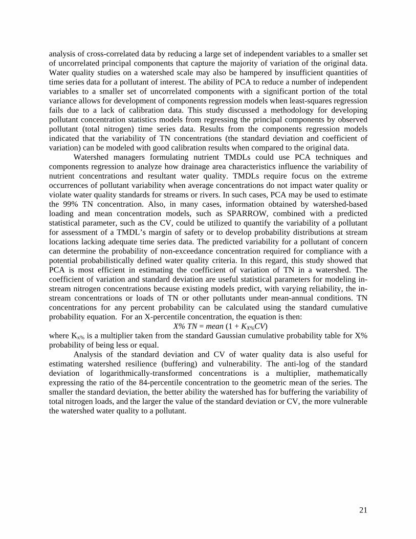
Total Nitrogen Monitoring Data The Great and Little Miami Rivers Basin is one of fifty study units selected by USGS NAWQA for water quality and ecology monitoring and analysis of surface and groundwater resources. The watershed contains numerous USGS stations with multiple hydrologic and water quality measurements. Such data can be retrieved from the USGS data warehouse4. The parameter of concern is Total Nitrogen, the sum of ammonium, organic nitrogen, nitrite and nitrate as nitrogen. The extreme 99% probability of non-exceedance of TN concentrations for the monitoring stations was calculated using available time series data from the monitoring stations. Figure 3.1 displays the Great and Little Miami Rivers Watershed in southwest Ohio and the locations of the monitoring stations inside the watershed.
Figure 2.1 Map of the watershed with the monitoring sites
4 water.usgs.gov
17
Watershed Characteristic And Nutrient Source Data The Enhanced River Reach File (ERF) version 1.2 from 1999 was used as a digital source
of rivers and streams in the study watersheds (USGS, 1999). The ArcHydro hydrologic extension for ESRI ArcGIS software was used to condition the US Geologic Survey National Elevation Dataset (NED) elevation data (USGS, 2003) and delineate drainage areas for each monitoring station in the study watersheds (Maidment, 2002). The Natural Resources Conservation Service (NRCS) State Soil Geographic (STATSGO) database was used as a source of soil permeability data (NRCS, 2005). Land cover statistics were generated for the delineated drainage areas using USGS National Land Cover Dataset (NLCD) land cover raster datasets based primarily on 1992 Landsat data (USGS, 1992). Land use classes for this study were based on groupings of the 21 land cover modified Anderson Land Cover classifications: cultivated, forested, urban, and wetlands. Also, land use statistics were calculated for the total contributing 300-meter riparian buffer areas around streams draining to the monitoring station locations. USGS Spatially Referenced Regressions on Watershed Attributes (SPARROW) National Nutrient Models results were used as a source of percent contribution data for various TN sources and stream flow data in the study watersheds. SPARROW is a nonlinear regression model with stochastic and deterministic properties (Smith et al., 1997).
The predominant land cover type in the delineated drainage areas was cultivated land use. While the overall trends in land use were similar in the total and buffer drainage areas, the percentage of cultivated land in the buffer drainage areas was typically less in magnitude. Forest and wetland areas were more prevalent in the riparian buffer areas for both study watersheds. Agricultural fertilizer had the largest contribution to TN loads at all monitoring points. Point source TN contributions were larger in drainage areas with higher percentages of urban land.
The watershed data was generated for total drainage area to each monitoring station. The basic overall land cover trends in the study watersheds (predominately agriculture with minimal wetlands) have been consistent during subsequent monitoring periods (Debrewer et al., 2000). Methodology
Principal Components Analysis In hydrologic or water quality modeling, least-squares regression fails to produce
accurate results when independent variables are cross-correlated. In such cases, multivariate modeling may be required. McCuen and Snyder (1986) and Kendall (1957) demonstrated that principal components analysis (PCA) can reduce the effects of cross-correlated variables by creating statistically independent variables, or components, by rotating original data vectors to orthonormal axes. Eigenvalue-eigenvector analysis of a correlation matrix for original water quality variates results in a set of coefficients, or loadings, relating the original variates to the components. The amount of variance in the original data contained by the components is represented by their corresponding eigenvalues; components and their respective variances may be summed. In effect, PCA reduces a number of water quality or hydrologic variates to a smaller set of uncorrelated principal components, representing a significant portion of the variation of the original data.
This study used PCA to analyze significant correlations among the independent variables. PCA reduced the 15 selected watershed variables to principal components that accounted for
18
92% of the total variance of the original data. The variation of the original variable data set was examined by analyzing the significant variable loadings to the principal components.
Components Regression Components regression includes the ability to sum regression coefficients and the square
of the correlation coefficient for sets of components. This feature allows the structure of models to be analyzed as components and additional variance are added to the correlation with the TN data. Regression equations were developed from the principal components to create components regression models capturing at least 90% of the total variation in the original data. Components regression models were generated to predict an extreme (99% probability of non-exceedance) TN concentration, mean TN concentration, the standard deviation of TN data, and the coefficient of variation (CV) of TN data.
Results and Discussion
Principal Components Analysis For this study, PCA was performed using MATLAB to calculate correlation coefficient
matrices and eigenvalues (variance) and eigenvectors (variable loadings) for the principal components. The matrices were analyzed for any strong correlations between variables. The land use statistics for total drainage areas had very high correlation coefficients in relation to the same riparian buffer land use statistics, indicating that land use patterns were consistent at both spatial scales. Strong negative correlations existed between the cultivated land use statistic variables and other land use types, which may be attributed to the prevalence of agricultural land uses. Wetlands exhibited positive correlations to forest land cover and negative correlations to cultivated land cover. Overall, PCA of the study watershed data resulted in moderate correlations between numerous variables, indicating some degree of cross-correlation in the dataset.
PCA reduced the 15 independent variables to seven principal components that accounted for 92% of the variation in the original data. The PCA components with their share of the variance of the data are described in Technical Report #2. For the Great and Little Miami Rivers data, the first principal component accounted for 30.75% of the total variation of the independent variables and was characterized by significant loading values from the land use variables, especially the cultivated and forested land covers. The second component contributed to 21.25% of the variation and had significant loadings from the urban land cover, as well as significant effects from point source and fertilizer TN inputs. Another 13.4% of the variation was captured by the third component, which was dominated by loadings from the atmospheric deposition TN input and the urban land cover. The fourth principal component contributed to 10.2% of the variance and it was set apart by strong loading from animal manure TN input, as well as being the only component with any significant effect from the wetlands land cover. Further, 6.8%, 6.23%, and 3.37% of the variance in the data were captured by the fifth, sixth and seventh principal components, respectively. These components were characterized by strong loadings from soil permeability, forested land cover, and cultivated land cover respectively.
In general, there weren’t much strong loadings from wetlands in the seven principal components, as wetlands are scarce in the study watershed with an average of 0.3% wetland land cover in the drainage areas of the monitoring stations and 0.63% in the riparian buffers. Figure 3.2 shows how the observed 99% TN varies with the wetlands land cover. From this figure, it
19
can be inferred that there is no specific trend for this variation. The percentage of wetland land cover in this study watershed may be below the threshold necessary to cause reductions in TN loads from high percentages of agricultural land use and associated TN sources such as fertilizers and animal wastes. However, the other land cover classes had a noteworthy effect at one point or another in one of the principal components with significant contribution to the total variance. Generally, the variables with the highest loadings were the land cover variables and the point source TN inputs. The variables with the weakest effects on the variance were the mean flow rate in the river and the watershed area, the pure hydrologic variables. This suggests that land use and agricultural practices are the factors affecting instream TN concentrations in the Great and Little Miami Rivers watershed, and not the hydrology of the watershed. The lack of correlation and the erratic behavior can be easily noted in Figure 3 which shows a plot of the observed 99% TN with the drainage area at the 46 monitoring stations.
Figure 2 – Observed 99%TN versus the wetlands land cover
Components Regression Models The components regression models were created by fitting the principal components to
the TN monitoring data statistics. Analysis of these equations revealed that the structure of the mean TN concentration model for the Great and Little Miami Rivers differed significantly from the extreme TN model, indicating that some watershed factors may influence the mean-annual loadings of TN differently than the extreme TN loadings in the watershed.
Analysis of the calibration results (R2-values) for comparison of the original TN data versus modeled statistics indicated that the models for CV and 99%TN were the best calibrated models with R2 of 0.71 and 0.6 respectively. Figure 3.4 displays the results for CV. The fact that the far best correlation was obtained for CV = standard deviation/mean indicates that the magnitude of the variability parameters is proportional to the sample mean which depends on different parameters than those that predict variability.
20
The entire calibration results of models are in Technical Report #2. The analysis reveals the second component is the one with the largest contribution to the R2 values. The importance of the second principal component suggests that urban land covers and point source TN inputs exerted the highest influence on TN predictions from component regression for this study watershed. However the urban land cover in the watershed was relatively scattered and sparse, averaging 7% in the drainage areas, which suggests that instream TN is sensitive to urbanization.
Figure 4 – Calibration Plot for Components Regression Model of CV of TN Data
Summary of Results and Conclusions
In the PCA of the Great and Little Miami Rivers Watershed, the first and second principal components accounted for 52% of the variability in TN concentrations. The variables with strong loadings into these two components are the cultivated, forested and urban land covers (at both the watershed and the 300 m buffer scales) and the point source and fertilizer TN inputs. Wetlands land cover and hydrologic variables such as the stream mean flow rate and the drainage area had no significant impact on the variability. The first principal component accounted for higher variability than the second but the latter had the largest R2 value in the components regression. Thereby it can be concluded that the cultivated and forested land covers have more influence on the variability of TN concentration but the value of the concentration itself depends more on the urban land cover in the watershed, despite the prevalence of cultivated land cover and lack of urban centers in the study watersheds. Calibration of components regression equations was most accurate with the coefficient of variation (CV) and the 99% TN.
Studies addressing water quality problems impacted by multiple watershed factors may be affected by cross-correlated independent variables. Multivariate statistical methods, such as principal components analysis, can recognize correlations that exist between numerous watershed characteristics, land use, and pollutant source variables. The use of PCA aids the
21
analysis of cross-correlated data by reducing a large set of independent variables to a smaller set of uncorrelated principal components that capture the majority of variation of the original data. Water quality studies on a watershed scale may also be hampered by insufficient quantities of time series data for a pollutant of interest. The ability of PCA to reduce a number of independent variables to a smaller set of uncorrelated components with a significant portion of the total variance allows for development of components regression models when least-squares regression fails due to a lack of calibration data. This study discussed a methodology for developing pollutant concentration statistics models from regressing the principal components by observed pollutant (total nitrogen) time series data. Results from the components regression models indicated that the variability of TN concentrations (the standard deviation and coefficient of variation) can be modeled with good calibration results when compared to the original data.
Watershed managers formulating nutrient TMDLs could use PCA techniques and components regression to analyze how drainage area characteristics influence the variability of nutrient concentrations and resultant water quality. TMDLs require focus on the extreme occurrences of pollutant variability when average concentrations do not impact water quality or violate water quality standards for streams or rivers. In such cases, PCA may be used to estimate the 99% TN concentration. Also, in many cases, information obtained by watershed-based loading and mean concentration models, such as SPARROW, combined with a predicted statistical parameter, such as the CV, could be utilized to quantify the variability of a pollutant for assessment of a TMDL’s margin of safety or to develop probability distributions at stream locations lacking adequate time series data. The predicted variability for a pollutant of concern can determine the probability of non-exceedance concentration required for compliance with a potential probabilistically defined water quality criteria. In this regard, this study showed that PCA is most efficient in estimating the coefficient of variation of TN in a watershed. The coefficient of variation and standard deviation are useful statistical parameters for modeling in-stream nitrogen concentrations because existing models predict, with varying reliability, the in-stream concentrations or loads of TN or other pollutants under mean-annual conditions. TN concentrations for any percent probability can be calculated using the standard cumulative probability equation. For an X-percentile concentration, the equation is then:
X% TN = mean (1 + KX%CV) where Kx% is a multiplier taken from the standard Gaussian cumulative probability table for X% probability of being less or equal.
Analysis of the standard deviation and CV of water quality data is also useful for estimating watershed resilience (buffering) and vulnerability. The anti-log of the standard deviation of logarithmically-transformed concentrations is a multiplier, mathematically expressing the ratio of the 84-percentile concentration to the geometric mean of the series. The smaller the standard deviation, the better ability the watershed has for buffering the variability of total nitrogen loads, and the larger the value of the standard deviation or CV, the more vulnerable the watershed water quality to a pollutant.
22
23
IV FRAGMENTATION OF AGRICULTURAL LANDS AND IMPACT OF LAND USE TRANSFORMATION ON STREAM IBI IN SOUTHEASTERN WISCONSIN5
Introduction The research by the University of Wisconsin team developed a method for examining the
impact of transitioning landscape of exurbia utilizing the theory and practices established within the field of landscape ecology. The overall objectives were: (1) to identify a subset of metrics that capture the majority of variation in agriculture land fragmentation in southeastern Wisconsin, and (2) to identify a subset of metrics that capture the relationship between agricultural land fragmentation and a measure of biotic integrity (IBI: an index score based on fish population variables). In order to accomplish the goals, landscape metrics were calculated and statistically analyzed to identify the most important landscape metrics that explained most of the variation in aquatic environmental integrity. Dynamic conversion of agricultural lands to low-density residential land use beyond the urban fringe (exurban) is a less studied aspect that affects the integrity of suburban streams. Exurbanization is considered the fastest transitioning form of landscape development in the United States (Crump, 2003; Theobald, 2002; Daniels, 1999). The change in landscape configuration resulting from appropriation of agricultural lands for exurban development can have a variety of ecological effects. Conversion of agricultural lands to residential lands may alter environmental integrity through a range of processes including: fragmenting landscapes, isolating habitat patches, simplifying biodiversity, degrading natural habitats, modifying landforms and drainage networks, introducing exotic species, controlling and modifying disturbances (e.g., floods, forest fires), and disrupting energy flow and nutrient cycling (Alberti, 2005; Alberti et al., 2003; Pickett et al., 2000).
Today more than 70% of the US population lives in urbanized areas; however, the rapid growth of exurbs indicates that many US citizens find rural environments appealing (Crump, 2003; Morrill, 1992; Nelson, 1992). Studies suggest a substantial preference for exurban locations among much of the US population. For example, Blackwood and Carpenter (1978) surveyed 1,400 residents of urban Arizona to find out where they would prefer to live and what factors they liked best. More than 66% of the respondents favored rural counties with populations less than 50,000. Additionally, 41% stated they would prefer to live in a town with less than 10,000 people. When asked to rate which factors were most influential for choosing rural or small town locations, the participants chose population size and environmental quality (Blackwood and Carpenter, 1978).
This study investigated the spatial configuration of agricultural lands in relation to exurban development and ecological integrity in southeastern Wisconsin. Specifically, 31 watershed delineated landscapes were used to investigate the environmental effects of fragmented agricultural lands associated with exurban growth.
Development affects the natural ecosystems by: fragmenting landscapes, isolating habitat patches, simplifying biodiversity, degrading natural habitats, modifying landforms and drainage networks, introducing exotic species, controlling and modifying disturbances, and disrupting energy flow and nutrient cycling (Alberti, 2005; Alberti et al., 2003; and Pickett et al., 2000). In
5 See Technical Report # 11 for details
24
response to analyzing and understanding the transitioning landscapes of exurbia, theory and practices established within landscape ecology were used.
Background Landscape ecology, as defined by Richard T. T. Forman, (1983) incorporates: (1) the
spatial relationship among landscape elements, or ecosystems, (2) the flow of energy, minerals, nutrients, and species among the elements, and (3) the ecological dynamics of the landscape mosaic through time. Today, landscape ecology is considered to be an interdisciplinary science drawing from a variety of different disciplines (i.e., anthropology, architecture, biology, ecology, economics, geography, and forestry). A key component of landscape ecology addresses anthropogenic effects on both natural and built landscapes; furthermore, understanding that human activity is a central factor for shaping the environment (Bissonette and Storch, 2003; Dramstad et al., 1996; Forman, 1995; Turner et al., 2001). Landscape ecologists have started to document the impacts that various arrangements of patch structure have on ecosystem function (Godron and Forman, 1982; Turner, 1989; Forman, 1995; Collinge, 1996).
A patch, as defined by Richard Forman (1995), is an area of specific type (e.g., agricultural field, woodlot, lake) that is different than its surrounding types in a landscape. The size and shape of the patch, its proximity to other patches, and its edges are particularly important patch characteristics that have significant ecological and environmental impacts (Forman, 1995; Turner et al., 2001; Alberti 2005). The patch is the primary component in landscape ecology used for developing the analytical metrics in a land cover or land use analysis. Exurbia provides ecologists with an opportunity to examine the urbanization process as a transformation of landscape patterns and functions (Bessey, 2002; Huang, 1998). One approach is to characterize the relationships between various arrangements of patch structure and ecosystem functions (Godron and Forman 1982; Turner 1989; Forman 1995; Collinge 1996).
With literally hundreds of landscape ecology metrics available, it is imperative to address several questions when using landscape metrics in assessment efforts: (1) What are the objectives of the study; (2) What is the behavior of the metrics over a range of landscape configurations; (3) What are the effects of scale on the metrics; and (4) are the metrics correlated or redundant (Turner et al. 2001)? In some instances, efforts to study landscape fragmentation have used artificial landscapes in their analysis (Gustafson and Parker, 1992; Hargis et al., 1998). In this analysis, a set of real landscapes are used to synthesize independent metrics into an overall measure of agriculture fragmentation, an explanatory model of exurban development, and a predictive model of environmental quality.
Land Use, Watersheds, and Biological Integrity The catchment or watershed paradigm started in the mid 1970s changed the way stream
ecologists look at the landscape. “In every respect, the valley rules the stream” (Hynes, 1975). “Rivers and streams serve as a continent’s circulatory system, and the study of those rivers, like the study of blood, can diagnose the health not only of the rivers themselves but of their landscapes” (Sioli, 1975). Since then, rivers have been studied from a landscape perspective, both as individual landscapes (Robinson et al., 2002, Ward, 1998, Wiens, 1989), and as ecosystems that are strongly influenced by their surroundings at multiple scales (Townsend et al.,
25
2003; Fausch et al., 2002; Allan et al., 1997; Schlosser, 1991). Increased attention to the landscape perspective of rivers continues to evolve with the growth of landscape ecology as a field of study (Turner et al., 2001; Wiens, 1989) and because of an increased focus on catchment-scale studies by freshwater ecologists (Allan, 2004).
Researchers have investigated the effects of land use or land cover on biological processes, leading to significant work exploring ecological regions (Heilman et al., 2002), buffer areas (Wang et al., 2001), Landsat image boundaries (Tinker et al., 1998), hexagonal units (Griffith et al., 2000), and watersheds boundaries (Potter et al., 2005; Cain et al., 1997) for dividing the landscape. In all cases, the physical characteristics of streams that shape biotic communities are influenced by a variety of landscape features, including geology, catchment area, and land use (Richards et al., 1996). Based on the demonstrated ability of watersheds explaining a greater amount of variability in aquatic ecosystems (Potter et al., 2005; Sliva and Williams, 2001; Wang et al., 2000; Weigel, 2000; Roth et al., 1996; Allan, 1995); this study uses watersheds to separate the study area of southeastern Wisconsin into 31 individual landscapes. There have been many terms used to describe or capture the status of river system, such as ecological integrity, stream condition, and river health. Typically, the ideas behind these terms were motivated by a desire to characterize a stream’s response to human influences (Allan, 2004). When assessing river health, several indicators, such as the number of intolerant species and taxa richness [Index of Biologic Integrity (IBI), see Karr, 1991have been used. The number of observed taxa related to the expected can be used [Rivpacs, see Wright 1995; Ausrivas, see Norris & Hawkins, 2000). Additional measures include: taxa richness of sensitive species; body size and shape, life history, and behavioral traits (Usseglio-Polatera et al., 2000; Corkum, 1999; Pan et al., 1999; Townsend & Hildrew, 1994); pollution tolerance (Hilsenhoff, 1988); and ecosystem processes, such as photosynthesis and respiration (Bunn et al., 1999). Habitat and water quality measures using individual variables or combined metrics are also available (Barbour et al., 1999). Thus, a plethora of methods are available for assessing the response of stream condition to land use or land cover.
Investigating agricultural fragmentation as an indication of development and linking agricultural fragmentation to an Index of Biotic Integrity (IBI) will be very valuable to the science community and planners alike. A primary objective of this analysis is to examine the relationship between agricultural fragmentation metrics and fish IBI, and to evaluate fragmentation as an indicator of environmental quality in warm water streams for southeastern Wisconsin.
Coupling Agricultural Landscape Metrics and Biotic Integrity
With the advancement of numerous methods for evaluating ecosystems, combined with technological increase in geographic information systems and spatial analysis, a plethora of works linking land use/land cover to river condition has developed. Specifically, when investigating agricultural effects, a decline in water quality, habitat, and biological assemblages occurred as the extent of agricultural lands increase within the catchments (Richards et al., 1996; Roth et al., 1996; Wang et al., 1997; Skinner et al., 1997; Sponseller et al., 2001). Further, researchers commonly report that streams draining agricultural lands support fewer species of sensitive insect and fish taxa than other forms of land cover (Cooper, 1993; Lenat and Crawford, 1994; Wang et al., 1997; Genito et al. 2002). With the advancement of this type of research, the ability to improve science-based conservation and management of rivers also improves. It has
26
been stated by Allen (2004) that the catchment approach to the management of river ecosystems can be conceived of in four steps: (1) identify the land-water unit, (2) asses the status or “health” of the river, (3) identify the stressors that influence the river status, and (4) develop management and restoration plans, grounded in good ecological science, to reverse or mitigate impacts.
Even with the availability of calculating landscape metrics through available software such as FRAGSTATS (McGarigal and Marks, 1995) linkages to ecological process and function remains largely untested (Allen, 2004; Alberti et al., 2003; Pickett et al., 2001; Grimm et al., 2000). Additionally, studies associated to the urban – rural gradient are often simple transects and miss the complexities of landscape patterns emerging by the distribution of land use and land cover (Alberti, 2005). In order to combat the paradox of limited landscape ecology research on ecological function and process, the fragmentation of agricultural lands in southeastern Wisconsin will be compared to the Wisconsin Index of Biotic Integrity (IBI). By studying agricultural land fragmentation in Southeastern Wisconsin, the interactions between human processes and biological complexities in exurbia are investigated. Specifically, this research links agricultural land fragmentation to the fastest transitioning landscape of exurbia, with a measure of environmental quality, that can be used for watershed management and planning.
Study Area Description Upon settlement, most of southeastern Wisconsin’s native prairies were transformed into
agricultural lands. Those agricultural lands remained the hallmark of southeastern Wisconsin until shortly after WWII. Soon after WWII population growth outside of urban centers began to increase rapidly. From post WWII to the present, agricultural lands have continued to decline as residential development boomed and populations increased beyond the metropolitan fringe. Today, southeastern Wisconsin is vital to Wisconsin due to its large population, urban centers, and remaining agricultural lands. This analysis of agricultural land fragmentation examined 31 watersheds crossing 15 counties of southeastern Wisconsin (Figure 4.1). Those counties (Green Lake, Fond du Lac, Sheboygan, Columbia, Dodge, Washington, Ozaukee, Dane, Jefferson, Waukesha, Milwaukee, Rock, Walworth, Racine, and Kenosha) had a population of 2,547,635 in 1970 which grew to 2,953,174 by 2000; an increase of 14 % (405,539 people) over a span of 30 years (United States Census 2000). Much of this growth has occurred in counties primarily dominated by agricultural lands surrounding Madison and Milwaukee. The 15 counties used for this analysis had 4,250,000 acres of farmland in 1970 which decreased to 3,261,000 acres of farmland by 2000, a loss of 23 % (989,000 acres) over a span of 30 years (NASS 2000). Population increase and agricultural land decrease between 1970 and 2000 are listed in Table 1 and Table 2, respectively, for the counties in the study area. The State of Wisconsin has made efforts (e.g., smart growth initiatives) to control rural population growth related to urban sprawl, but it is likely that further fragmentation of the state’s agricultural lands will occur. Mapping the fragmentation of southeastern Wisconsin’s agriculture lands is critical to protecting terrestrial and aquatic ecosystems and controlling the environmental affects of human population growth.
Data The land cover data set used in this analysis is titled: WISCLAND Land Cover
(WLCGW930). It was developed for the Wisconsin Department of Natural Resources (WIDNR) as part of a larger project for the Upper Midwest Gap Analysis Program (UMGAP) Image Processing Protocol (1998). The dataset was published for use in Wisconsin in 1998, and is available online in Geographic Information System (GIS) compatible format from the WIDNR
27
at: http://dnr.wi.gov/maps/gis/datalandcover.html. The WISCLAND Land Cover data set is a raster representation of vegetation and land cover for the entire state of Wisconsin that was acquired from the larger national Multi-Resolution Land Characteristics Consortium (MRLC) data set.
Figure 4.1 Location of watersheds within southeastern Wisconsin
The MRCC created the data set for UMGAP using dual-date Landsat Thematic Mapper (TM) imagery data primarily from 1992. The original pixel size of the TM source data is 30 meters; however, excluding urban areas, data was generalized to an area no smaller than four contiguous pixels (approximately one acre). The results of the smoothing process will allow any feature five acres or larger to be resolved in the data, giving a Minimum Mapping Unit (MMU) of five acres. During the generalization process the data set was transformed from its original raster format into a more user-friendly vector format. With this MMU the data set is designed to be used between scales of 1:40,000 to 1:500,000 for a wide variety of resource management and planning applications.
The land cover classification scheme was designed to be compatible with the UNESCO and Anderson’s classifications and included six land cover classes associated with it: (1) agricultural land, (2) barren land, (3) forest land, (4) urban/built-up land, (5) water, and (6) wetland. Both the agricultural land fragmentation data derived from the WISCLAND Land
28
Cover (WLCGW930) and the 10-digit Hydrological Unit Hierarchy (HUC) were utilized in investigation of the relationship between agricultural land fragmentation and measure of environmental quality.
Fish Biological Data The Wisconsin version of fish IBI is a modification of the original Index of Biotic
Integrity developed by Karr et al. (1986). Wisconsin IBI consists of 12 metrics that can be simplified into three categories (see Technical Report # 11 Shaker and Ehlinger, 2007)). The index was created to capture variation of species in a community in relation to variation in the environmental quality in the watershed (Lyons, 1992). The IBI data used in this analysis were collected by and obtained from the Wisconsin Department of Natural Resources. The samples were collected over a span of four years (2001-2005) and were used to provide an average score per sample site. In the study area, 152 fish IBI sites were used to investigate the effects agricultural fragmentation is having on a measure of environmental quality for southeastern Wisconsin (Figure 4.2).
Figure 4.2 Location of the 162 fish sampling sites and the ranges of measured IBIs in the 31 watershed located in sSoutheastern Wisconsin
Methods
Calculation of Landscape Metrics Geographic Information System (ESRI ArcGIS 9.1) separated the 31 watersheds into their individual shapefiles from the original 334 subwatersheds. The raster format was used for the analysis in the landscape ecology software FRAGSTATS 3.3 (McGarigal and Marks, 1995, available at http://www.umass.edu/landeco/research/fragstats/fragstats.html). Because the
29
original land cover data were collected at 30-meter resolution, the pixel size for the conversion process was kept at 30 meters by 30 meters.
In order to determine the metrics that best characterize the arrangement of agricultural lands for southeastern Wisconsin, 72 FRAGSTAT metrics were calculated using a sample of 31 individual watershed landscapes of roughly 3,525 ha. Class metrics in FRAGSTATS are computed for every patch type or land cover class in the landscape. There are two basic types of metrics at the class level: (1) indices of the amount and spatial configuration of the class, which can be referred to as primary metrics, and (2) distributional statistics that provide central tendency (e.g., mean and area weighted mean) and variance (e.g., standard deviation and coefficient of variation) statistical summaries of the patch metrics for the focal class (McGarigal and Marks, 1995). Metrics were normalized by either log10 or arcsine transformation. Pearson correlation coefficients test to determine and eliminate highly correlated (|r| > 0.90) metrics using SPSS 13 (SPSS, 2003). Results representing primary metrics or central tendency metrics were selected first, because they are considered to represent high or low agricultural land fragmentation. Fifty of the original 72 landscape ecology metrics remained after running the Pearson correlation coefficients test. A summary of the class level metrics and methodology is found in the Technical Report 11 (Shaker and Ehlinger, 2007).
The database of normalized agricultural metrics per watershed was joined with the database of the 152 fish sites and an average IBI score was calculated for each watershed (Figure 4.3). Forward-stepping stepwise multiple regression (SYSTAT 12.0) was used to select the best set of the 50 normalized agricultural land fragmentation metrics that predicted the average Fish IBI score per watershed. This resulted in the selection of 6 agricultural fragmentation metrics. Finally, for each of the landscape regions (i.e. watersheds), the 6 remaining metrics were weighted by their respective contribution to the change in R-square change and summed to generate an index of agriculture fragmentation that predicted average fish IBI in a watershed.
Results
Stream Environmental Quality Model Using the matrix of Pearson correlation coefficients (|r| > .90) 22 of the original 72
metrics were eliminated (see Technical Report # 11 for listing of metric). Of the 22 metrics eliminated 5 (23%) were primary metrics, 8 (36%) were central tendency metrics and 9 (41%) were variance metrics. Of the 50 retained metrics, 20 (40%) were primary metrics, 16 (32%) were central tendency metrics (i.e., mean or area weighted mean), and 14 (28%) were variance metrics (i.e., standard deviation or coefficient of variation).
Stepwise multiple regression eliminated 44 of the remaining 50 agricultural metrics. Of the remaining agricultural land fragmentation metrics three were primary metrics, two were central tendency metrics, and one was a variance metric (Table 4.1). The three primary metrics of Area/Edge Density were included: Largest Patch Index (LPI), Total Class Area (CA), and Normalize Landscape Shape Index (NSLI). One central tendency metric for Shape, Area Weighted Mean Shape Index (SHAPE_AM) and one variance metric for shape, Standard Deviation of Mean Fractal Dimension Index (FRAC_SD), were included. One primary metric for Proximity/Isolation, Mean Euclidian Nearest Neighbor Index (ENN_MN) was included. Largest Patch Index (LPI) is equal the area of the largest patch of agricultural land divided by the total landscape area, multiplied by 100 to create a percentage (McGarigal and Marks 1995).
30
LPI at the class level quantifies the percentage of total landscape area comprised by the largest patch; LPI can be considered as a simple measure of dominance. Class Area (CA) equals the sum of the areas of all the agricultural land patches, divided by 10,000 to create hectares (McGarigal and Marks, 1995). CA is a measure of landscape composition; specifically, how much of the landscape is comprised of the agricultural land type. Area Weighted Mean Shape Index (SHAPE_AM) equals agricultural patch perimeter divided by the minimum patch perimeter in the landscape; further the shape scores are divided by the sum of all shape scores in the landscape (McGarigal and Marks, 1995). CORE equals the area within the patch that is further than the specified depth-of-edge distance from the patch perimeter, divided by 10,000 (to convert to hectares). Euclidean nearest-neighbor distance is perhaps the simplest measure of patch context and has been used extensively to quantify patch isolation. Here, nearest neighbor distance is calcuated using simple Euclidean geometry as the shortest straight-line distance between the focal patch and its nearest neighbor of the same class. Fractal dimension index indicates a departure from Euclidean geometry (i.e., an increase in shape complexity). FRAC approaches 1 for shapes with very simple perimeters such as squares, and approaches 2 for shapes with highly convoluted, plane-filling perimeters.
Table 4.1. Results of stepwise multiple regression average stream biological integrity in a watershed (AVBG_FISHIBI) as a function of agricultural fragmentation landscape metrics. (A) Final regression model showing standardized coefficients, (B) Analysis of variance for overall significance of final model.
The relationship between IBI Score and the six metrics: LPI, CA, ENN_MN, FRAC_SD,
NLSI and SHAPE_AM explained 84 % of the variation in IBI among the watersheds. Positive effects on IBI included measures of fragment size and isolation. The strongest positive influence of an individual agricultural land fragmentation metric in predicting the IBI score was Largest Patch Index (LPI, std. coeff. = 0.74, p < .001, Figure 4.3). Other positive influences on IBI included Total Core Area (CA, Figure 4.4) and Mean Euclidean Nearest Neighbor (ENN_MN). The combined effect of these three factors indicates that larger patches of contiguous landscape further apart contribute more to environmental quality than smaller patches closer together. The
EffectStandard
Coefficientt p-value
CONSTANT 0.00 -5.03 0.00
LPI 0.74 4.89 0.00
CA 0.57 5.11 0.00
ENN_MN 0.24 2.18 0.05
FRAC_SD -0.27 -2.59 0.02
NLSI -0.34 -2.18 0.05
SHAPE_AM -0.55 -4.68 0.00
B. Analysis of Variance
Source SS dfMean
SquaresF-ratio p-value
Regression 652.01 6.00 108.67 13.34 0.00
Residual 122.24 15.00 8.15
Dependent VariableAVG_FISHI
B
N 22
Multiple R 0.92
Squared Multiple R 0.84
Standard Error of Estimate
2.86
A. Standardized regression model
31
three metrics that had a negative contribution to IBI were measures of variability in landscape patch shape and size. The strongest negative contribution was from Weighted Mean Shape Index (SHAPE_AM, std. coeff. = 0. 55, p < 0.001, Figure 4.4), followed closely by Normalized Landscape Shape Index (NLSI) (Figure 4.5) and Standard Deviation of Mean Fractal Dimension Index (FRAC_SD). This combination of negative effects indicates that increased complexity and variability in patch shape within watersheds contributes lower aquatic biological integrity.
A plot of empirically measured IBI versus that predicted from the landscape metrics is presented in Figure 4.6. The landscape fragmentation model is significantly better at predicting aquatic biological integrity in exurban environments compared to the more often-used metric of urbanization.
Discussion Few articles in the literature have established strong predictive models that go beyond
simplistic relationships of the IBIs to one or a few parameters. Percent of imperviousness is a surrogate for many adverse stresses caused by urbanization and development (Wang et al, 2000). The results of this study indicate that a strong relationship exists between biotic integrity and the spatial arrangement and shapes of development in exurban watersheds that goes beyond simply the amount of a particular type of development. This research selected a suite of four metrics from an initial 72 metrics that best represent patterns of agricultural land fragmentation and produced a viable method for determining agricultural land fragmentation patterns and creating an overall index for southeastern Wisconsin. The findings in this research were consistent with the literature. Measures of core area (LPI and CA) represent the first two factors in the model. These two measures, representing patch size and dominance, accounted for the largest coefficients for positive effects on IBI. Measures of patch shape and complexity (SHAPE_AM and FRAC_SD) represented greatest negative impacts on biological integrity. Finally, a measure of proximity/isolation (ENN_MN) suggested that the distance between landscape patches is a significant factor impacting aquatic ecosytems.
In summary, this approach of creating an agricultural land fragmentation index and exurban development model is a practical method that can be replicated in other regions. The results of doing such research can be useful to ecologists, natural resource managers, and planners alike. Agricultural land fragmentation information has been typically underestimated because ground-based measurements of land-use change are difficult (Riebsame, Gosnell, and Theobald, 1996; Theobald, Gosnell, and Riebsame, 1996). The fragmentation of agricultural lands has many negative and often irreversible effects such as the change in water chemistry, biodiversity, and increased flooding (Alberti, 2005; Theobald, 2002; Daniels, 1999). The relationships identified in this study provide an effective and efficiently tool for measuring and monitoring agricultural land fragmentation and may lead to informed recommendations for future planning and conservation efforts.
Studies such as this, coupled with remote sensing and GIS techniques, make it possible to monitor current conditions and predict changes. Measurement of agricultural fragmentation within landscape regions is a key step to understanding impacts of differences and change, and ultimately making wise planning decisions. By calibrating landscape metrics to a measure of environmental quality, in this case fish IBI, a surrogate or proxy method of measuring environmental quality can be further developed, refined and replicated in other region
32
Figure 4.3 Map of largest patch index (LPI) Figure 4.4 Map of total class area (CA)
Figure 4.5 Map of area weighted mean shape index (SHAPE_AM) metric
Figure 4.6 Plot of observed Fish IBI in the study watersheds predicted from multiple regression of landscape fragmentation metric
Introduction The team acquired and worked with large databases from several states. The larger databases contained measurements from up to 2000 sites that contained raw fish and macroinver-tebrate data, fish and macroinvertebrate IBI metrics (up to 12 each), and up to forty environmental variables such as habitat, chemistry, and land use. New advanced knowledge retrieval methods have become available in the last fifteen years for retrieval of knowledge and models from large multiparameter databases.
The hierarchical layered effect of progression of allochthonous and autochthonous stresses to risks to the integrity, and to the effects of internal habitat and chemical water and sediment risks on the integrity endpoints was advanced in Novotny et al. (2005). Risk progression begins with the landscape and pollution discharge allochthonous stresses divided into four categories: (1) landscape (e.g., imperviousness); (2) land use (e.g., agricultural, population density); (3) hydrologic/hydraulic (e.g., navigation, impoundments, change of hydrology by urbanization); and (4) pollutant loads. These allochthonous stresses at the bottom of the risk propagation pyramid; however, do not directly impact the biota, the main expression of integrity. Aquatic biota is impacted by in-stream (water body) stresses, such as habitat impairment (e.g., embeddedness, lack stream bank refuge, pool and riffle structure), and pollutant concentrations (risks) in water and sediments. Novotny et al. (2005) cautioned against using simplistic relationships and models relating indices of biotic integrity to a single stressor or even to multiple landscape stressors, of which the most popular one is percent imperviousness.
We developed an efficient data mining and visualization methodology for assessing the simultaneous effects of multiple anthropogenic stressors on the fish population through the fish metrics and habitat metrics. The methodology first uses Kohonen’s Self Organizing Maps (SOM) (Kohonen, 2001) and the k-means clustering algorithm (Duda et al., 2001) to partition sampling sites for the state of Ohio into groups based on similarity of their fish metrics characteristics. Canonical Correspondence Analysis (Ter Braak, 1986), a community ordination method popular in ecology, is then applied to assess how environmental variables are associated with the formed patterns. Different visualizations superimposed on the SOM are realized to explore the complex interrelationships in the aquatic system.
Self-organizing Maps The Self-Organizing Maps (Kohonen, 1990) is a popular neural network structure used
for data dimensionality reduction and clustering. In essence it performs a structure preserving, nonlinear projection of high-dimensional input data vectors onto the low-dimensional (usually 2D) space of neurons (see Figure 5.1). The data input vectors are presented multiple times one by one to the SOM network (multiple epochs). At presentation t, the input vector x(t) is compared with all the SOM neuron weights using some appropriate distance metric (e.g. the Euclidean distance, see Figure 5.1). The neuron with the shortest distance to the input vector is declared as the winning neuron, also called the Best Matching Unit (BMU). The weights of the BMU and its 6 See Technical Reports # 4 and 12 for details
34
neighboring neurons are then updated to further reduce the distance between them and the presented input vector. This has the effect of increasing the similarity of the presented data vector and the weights of the neighboring neurons. The same steps are repeated till convergence or for a fixed number of epochs. Using competitive learning, the SOM network encodes in its weights a low dimensional representation of the unknown input data distribution. Weights adaptation is achieved in an unsupervised manner, meaning that no “teacher output” is required. Several practical SOM applications are listed in Kohonen et al. (1996). However, SOMs have been sparsely used in ecology, although some successful cases have been reported recently (Gevrey et al., 2004; Park et al., 2004).
Figure 5.1 Principle of Kohonen’s Self Organizing Maps (Kohonen, 1990).
The size of the SOM map (number of output neuron units) has a strong influence on the
quality of the clustering. If the selected map size is too small, it might miss some important differences present in the data. Conversely, if the selected map size is too large, the differences may become too small to detect. Typically two quality criteria are used: resolution and topology preservation, assessed via the quantization and topographic errorsError! Reference source not found..The optimum map size was decided after considering both errors. A very high map size is undesirable and its size is determined from minimizes the topographic error while also resulting into a very small quantization error.
An initial impression of the number of neuron clusters present on the SOM and their spatial relationships can be acquired by visual inspection of the map. The U-matrix is a representation of the trained SOM that helps visualizing inter-neuron distances while also revealing potential neuron clusters present on the map. For the MBSS fish data, the calculated U-matrix gives the visual impression that there exist three neuron clusters (Figure 5.2A). One covering the bottom-right region, another covering the top-right region and a third one concentrated on the middle-left region of the map. Using the k-means clustering algorithm and the Davies-Bouldin index, which is a function of the ratio of the sum of within-cluster scatter to the in-between-cluster separation, it was confirmed that three is indeed the optimal number of
35
neuron clusters present in the map (Figure 5.2B). The steps of the k-means clustering algorithm are summarized in Technical Report # 4.
Figure 5.2. (A) Representation of the SOM U-matrix. The inter-unit values are the
Euclidean distances between adjacent map units. The levels of gray shown inside a specific unit are found by taking the median of the surrounding gray level values. A dark (light) shade between the neurons corresponds to a large (small) Euclidean distance and thus a large (small) gap between the codebook values in the input space. Therefore, light areas can be thought as neuron clusters and dark areas as cluster separators. The U-matrix visually suggests the presence of three groups of neurons (neuron clusters). (B) The three clusters extracted after applying the k-means algorithm (100 iterations) that largely agree with the clusters visible on the U-matrix (Fig. 5.2A).
Ohio Dataset and IBI fish metrics Ohio pioneered the integration of biosurvey data, physical habitat data, and bioassays
with water chemistry data to measure the overall integrity of water resources. The Ohio dataset analyzed in this research includes the chemical, habitat and biological data collected by the Ohio EPA between 1995 and 2000 (July to September). It consists of 1848 stations distributed over the entire state. Also, the time window for synchronising the dates for the chemical and the biological samples at a particular station was selected to be a week before or after, to capture the effects of the chemicals on the biota. We hypothesised that, in absence of toxic spills generating
36
fish kills (none reported) the water quality changes were relatively slow and a time span up to one week difference between the two types of information (biological and chemical) would still provide representative correlation between chemistry and fish composition. Other parameters such as habitat or land use change very slowly. Since the physical habitat was sampled once per year for a sampling station, the habitat data were duplicated to be accommodated in the dataset. The complete information regarding this dataset has been included in Technical Report # 4 (Virani et al. (2005) and in the Ohio EPA (1999) report. In the report, various exploratory tools such as box-and-whisker plots, scatter plots and multivariate techniques, such as Principal Component Analysis, were used to visualize regional patterns in nutrient concentration and relationships with biological performance parameters.
The Ohio EPA has formulated a list of 12 fish metrics (see Tech. Rep. # 4), modified from the ones proposed by Karr (1981), and based on the type of sites: Headwaters, Wading and Boat sites. Each type has a set of metrics to calculate the fish IBI (Ohio EPA, 1987). Karr (1991) eloquently described what the reasoning behind the selection of the metrics and selection of the type and fish genera were.. The IBI was not intended to be a quantitative measure of any specific pollution but of the overall impact of stressors and the “human disruption” and “degradation” were defined in generic terms. However, Karr’s (1991) article lists cases where other authors found correlations of IBIs to some specific disturbances, such as land use, and found them worth to be pursued in further research. Karr himself documented the effect of residual chlorine in the streams after effluent disinfection as one of the stressors significantly affecting IBI.
The original IBI defined by Karr at al (1986) and Karr (1991) uses three groups of metrics. The first group of six metrics evaluates the species richness and composition. The suckers, darters, and sunfish species feed on intervertebrates and are in the higher food web groups. Their numbers, normalized by the stream order, show the presence or absence of food (benthic or drifting organisms) which would reflect the degree of disturbance. The number of tolerant and intolerant species is expected to represent the degree of disruption with tolerant ones increasing and intolerant decreasing with the degree of pollution.
The next three metrics evaluate the trophic composition of the fish community and is used for assessment of the energy base and the trophic dynamics of the biota. The proportion of omnivores increases as the insectivorous and top carnivorous fish decrease in the degraded systems.
The last three metrics represent the fish abundance and condition. The number of fish is expected to decrease with the disturbance. The integrity can also be disrupted by invasive and hybrid species that are not indigenous to the area (e.g., the serious problem with exotic carp proliferation in the Mississippi and Illinois River watersheds widely reported by the media). The DELT (deformities, eroded fins, lesions, tumors) fish anomalies reflect the highest degree of disturbance typically related to severe disruption of integrity by high turbidity, temperature, and chronic effects of priority pollutants.
The IBIs are also related and compared to the reference streams or stream reaches which are the water bodies of the same character as the test site but least impacted by human stresses and disruption.
In the Ohio modification of the IBI the metric related to darters (DADSRNSCORE) combined a number (Number of Darter species at Headwater and Wading sites) and a percentage (Percent Round-bodied suckers at boat sites). The same is also true for SPWNSCORE, where the metric was composed of a number of simple lithophils species for headwaters and percentage of simple Lithophils for wading and boat sites. Since it would seem illogical to combine a number
37
and a percentage to represent the same metric, the metrics scores (ranked as 1, 3, and 5 from low to high) were used instead as the input to the SOM.
All data processing software was developed in MATLAB Version 6.5 (Matlab 2007). We have also utilized a public domain Matlab SOM toolbox developed at Helsinki University of Technology (Vesanto et al., 2000), which provides functions for data preprocessing, SOM training, and visualization of results.
The fish metrics were normalized using log transformation and linearly scaled in the range [0, 1]. The 12-dimensional normalized fish metric vectors (one per sampling site) were used as input data vectors to train an SOM. To find the optimal map size we considered a compromise between the topographic and the quantization errors (Kohonen, 2001). The quantization error is defined as the mean of the Euclidean distance of each data vector to its BMU’s weight vector and measures map resolution. The topographic error (Kiviluoto, 1996) is calculated as the proportion of all data vectors for which first and second BMUs are not adjacent units in the grid of neurons. Since a very large map size is undesirable (given the size of the data set), we decided to use 9 X 5 = 45 neurons, which minimizes the topographic error (0.02) while also resulting into a very small quantization error (0.85). Based on the 1848 sites analyzed this also implies that each neuron contained on an average information for about 40 similar sites. The SOM rough training phase lasted for 20 epochs, followed by the fine-tuning phase for another 100 epochs. Sites representing similar conditions, as judged by their similar fish metrics information, are mapped to the same SOM neuron after the training (site patterning).
The well known k-means algorithm (Duda et al., 2001) was then used to partition the SOM neurons into k groups (clusters) and assign a cluster label to each neuron. The algorithm initially places the k class centroids in randomly selected positions. Each point (neuron weight) gets associated with the closest cluster centroid. Then the centroid moves to the mean of the points it represents. Each time the class centroids move all data points are reclassified, and the same procedure is repeated until convergence. The Davies–Bouldin index (Davies et al., 1979), which is proportional to the ratio of the sum of within-cluster scatter to the in-between-cluster separation, was used to find the best value for k.
Figure 5.3 shows the SOM of the neuron clusters and ranges and whisker plots of IBIs in each cluster for Ohio. Visually, these clusters can be interpreted as Cluster I being very good, Cluster II as good and Cluster III as marginal. In reality, the clusters express the similarities of the IBI metrics and community structure rather than “goodness” of water quality or biota. It should be noted that the Ohio EPA has used simple ranges without SOM clustering to define the state biotic criteria. For example, in the Ohio biotic integrity classification, stream sections with IBI > 48 were ranked as exceptional warmwater habitats, 34 to 44 as typical warmwater habitat waters, and less than 30 as modified (poor) water bodies. More specific stream classification is related to the Ohio’s ecoregions. SOM cluster analysis can improve the logic of the criteria definition. Environmental variables related to water chemistry, physical habitat and land use, which were not used to train the SOM, were also mapped on the same SOM in order to shed light on the dependence of the fish metrics on these variables by comparing their maps. The gradient distribution of all the variables over 60 SOM neurons was used to calculate the correlation matrix. It is worth noting that these clusters approximately coincide with the Ohio biotic ranking of streams (Ohio EPA, 1987).
Figure 5.4 shows the spatial distribution of the sampling sites patterned in each cluster. Regions with poor fish IBI (in Cluster 3) are concentrated in the western part of Ohio, particularly around Toledo and along the Wabash River at the western state border. Almost all
38
small streams in the Toledo area have been channel modified to some degree (Yoder et al., 2000). The Wabash river watershed was designated as Ohio’s worst watershed by the Ohio EPA in 1999. Lack of buffer zones, excessive nutrient and high bacteria levels were attributed as some of the reasons for the poor conditions (Ohio EPA, 1999). The basins around Lake Erie, especially around Cleveland in the Cuyahoga County are also degraded.
Figure 5.3 Arrangements of ANN neurons in three clusters in for Ohio. The whisker plot indicates ranges of IBIs in the clusters.
Figure 5.4 Spatial distribution of monitoring sites throughout Ohio and their association with SOM clusters.
39
Each input data vector element has a weighted connection to each and every one of the SOM neurons (Figure 1). The value of this weight models the influence of an input element (fish metric) to the sites represented by an SOM neuron. The distribution of each fish metric on the SOM (Figure 5.5) can be visualized by the 2D map (called a component plane) of the corresponding weights. Visualization of the SOM through component plane representation provides us information about the correlations between individual components, division of data in the input space and relative distributions of the components. This figure shows that, for example, DELT score has low impact on the magnitude of the overall IBI. A weak effect can be also seen for the intolerant fish score metric. All other metrics exhibit similar pattern as the SOM for the total IBI.
Figure 5.5. Component planes for the metric scores visualized on the SOM (left) and corresponding whisker box plots (right) for the individual cluster distributions. There is a clear gradient distribution in most of the metric components. The ranges of the metric scores are shown in the corresponding color bar.
40
Figure 5.6 SOM visualization of habitat in the fish metric clusters. The impact of habitats is strong for SUBTRATE, EMBEDDEDNESS, COVER, CHANELization, RIPARIAN quality, GRADIENT, RIFFLE. Weak impact can be seen for PERcent Agriculture, PERcentURBan DEVelopment, PERcent FORested WETlands.
The habitat data have shown strong impact on and correlation with the fish IBI values and its metrics. Surprisingly, the effect of land use was not as strong as that of the channel and riparian zone quality.
The impact of chemistry was not as strong as that for some morphological channel and habitat quality. It was stronger for total suspended solids, iron and chlorides, medium for BOD, conductivity, DO, nitrate, TKN, sulfate, zinc and arsenic. The significant effect of iron could be explained by the impact of mining and former iron works in eastern Ohio that may be correlated to other stressors that have not been included in the database, for example, contaminated sediments. Elevated levels of arsenic impacted only Cluster (worst) III but showed no distinction between Clusters I and II. All other chemistry parameters had little impact on clustering of the IBIs and their metrics. Parameters with no impact included temperature, hardness (calcium and magnesium), and metals cadmium, copper, and lead. Very low phosphate was associated with Cluster I but there was little distinction in the effects of phosphate between clusters II and III.
41
Figure 5.7 Visualization of some chemistry data over fish SOM metrics. The ranges of the measured values are shown on the colored bar. The effect on fish IBI metrics is strong for TSS, TKN, and BOD but generally weak for the rest of the parameters. It is interesting and proper, using the values of the Invertebrate Community Index in the neuron and the clusters, to find similarities between the fish IBI and ICI. Figure 5.8 shows the k-value averaged ICIs in the three clusters. The ICI not only reflects the composition of the macroinvertenvate benthic community, it also serves as a surrogate for the sediment contamination. Figure 5.8 shows that that there is a similarity (correlation) between the two indices.
42
Figure 5.8 Distribution of the ICI on the SOM (left) and the corresponding boxplots (right) for the individual clusters. The different sizes of the neurons indicate the associated cluster for the neuron, whereby the largest (smallest) size indicates Cluster I (ClusterIII). Overall indicates that the data represents all the SOM neurons which cover data from the entire state. The color of each neuron corresponds to the mean value of the ICI of the sites contained in the neuron.
SOM Analysis for Maryland
The Maryland Biological Stream Survey (MBSS) was used as the second largest database to validate the applicability of the SOM/Canonical Correspondence Analysis methodology developed in this research This database has a large size and covers all three domains of variables of interest i.e. biological, chemical, and physical habitat. Furthermore, both raw fish and macroinvertebrate counts are available along with the values of the metrics scores. The complete list of all the variables used in MBSS is provided for quick reference in http://www.dnr.state.md.us/streams/mbss/ 12/2004). Extensive details can be found in Mercurio et al., (1999). Statewide and basinwide results and an assessment of the condition of the streams have been reported in the MBSS three-year report by Roth et al. (1999). It should be pointed out that the metrics used in calculating the fish IBI are not identical to the Ohio IBI; almost every state has been developing its own metrics.
A central goal for biological monitoring is to be able to distinguish between variation in biological integrity resulting from natural ecogeophysical differences (e.g. elevation and soils) and variation caused by human-induced factors (e.g. land cover changes and pollution inputs)Error! Reference source not found.. Again, three SOM clusters of the Maryland fish IBI were recognized by the analysis. Figure 5.9 presents the spatial distribution of the sampling sites falling within each cluster of neurons. Although sites from each of the three clusters occur throughout Maryland, they are not uniformly distributed (Figure 5.10). The sampling sites in Cluster 1 tend to occur more frequently either in the Youghiogheny basin in the west or in the Middle Potomac Basin in central Maryland. Sites belonging to Cluster 2 are predominant in the Piedmont Province. The coastal and southeastern plains are mostly populated with sites that
43
belong to Cluster 3. Comparison of SOM clusters (which were created “blind” to ecoregion location) overlaid by the calculated total IBI values shows that SOM captures variation among ecoregions (Table 5.11). Generally speaking, sites in Cluster 3 have lower scores for fish metrics and total IBI compared to Cluster 1, with sites in Cluster 2 exhibiting intermediate scores. Because of the lower gradient and naturally limited capacity to deoxygenate (decompose) the dissolved organic matter (BOD) and lower reaearation capacity, streams in the Coastal Plain more often tend to become more overenriched with less dissolved oxygen (DO) than elsewhere in the state .
Figure 5.9. (A) Representation of the SOM U-matrix. The inter-unit values are the Euclidean distances between adjacent map units. The levels of gray shown inside a specific unit are found by taking the median of the surrounding gray level values. A dark (light) shade between the neurons corresponds to a large (small) Euclidean distance and thus a large (small) gap between the codebook values in the input space. Therefore, light areas can be thought as neuron clusters and dark areas as cluster separators. The U-matrix visually suggests the presence of three groups of neurons (neuron clusters). (B) The three clusters of neurons extracted after applying the k-means algorithm (100 iterations) that largely agree with the clusters visible on the U-matrix (Fig. 5.9A). Again Cluster 3 is in the upper (red) part of the map, Claster 2 is in the middle and Cluster 1 (best) is in the lower part of the map.
The three clusters based on fish metrics in Maryland are not as distinct as the three in Ohio. This will be further elaborated by comparing the cluster identification based on habitat qualities which depicted more variability in the habitat conditions within this relatively small state.
44
Figure 5.10 (A) Spatial distribution of Maryland sampling sites belonging to each SOM neurons cluster extracted by using the k-means algorithm. Sampling sites in Cluster 1 are concentrated either in the western or in the central part of the State. The coastal area sites are mostly in Cluster 3. (B) Distribution of the fish IBI on the SOM (left) and the corresponding boxplots (right) for the individual clusters and the state overall. Three different patterns are used to visually separate the 3 clusters. The low values of the Fish IBI are concentrated in the top right area of the SOM (mostly including sites belonging to neurons of Cluster 3).
Table 5.1 Distribution of ecoregions in each cluster in Maryland. The percentages indicate the proportion of the sites in each ecoregion for each cluster.
The clustering also depicted the impact of stream order on the IBIs. Table 5.2 shows the worst IBIs (Cluster 3) were more associated with first order streams and least with 3rd order streams.
Table 5. 2: Distribution of the stream order in each cluster in Maryland. The percentages indicate the proportion of the sites in each cluster for a particular stream order.
Figure 5.11 shows the SOM metrics for Maryland. To complete the figure maps of mean values for two environmental variables, Dissolved Oxygen measured in the field (DO_FLD) and substrate embeddedness (EMBEDDED) are also shown in the bottom right part using the same representation. Any variable of interest could be selected and the overall or per-cluster distribution of a selected statistic could be visualized in a similar way. Figure 5.11 SOM of fish IBA metrics for Maryland with SOMs for Dissolved Oxygen and Embeddedness
46
Using weight component planes it can be seen that the metrics related to the percentage of Insectivores (PCINSECT) and the percentage of the group of Generalists, Omnivores and Invertivores (PCGOI) exhibit gradients in opposite directions. The metrics for the number of Native species (NUMNATIVE) and intolerant species (NUMINTOL) are mirror images of each other. Going from Cluster 1 to Cluster 3 in the boxplots, we see a gradual increase in the values for the metrics linked with tolerant species (PCTOL), while there is a gradual decline in the values for the metrics related to the Benthic species (NUMBENTHIC) and fish density (NUMINDVSQM). Metrics NUMNATIVE and NUMBENTHIC, which are associated with species richness, are expected to decrease in value in response to anthropogenic stress. Because many benthic fishes have relatively limited home ranges, they are potentially valuable indicators of local conditions. The density of individual fish count (NUMINDVSQM) and the biomass (BIOPSQM) are an indication of the overall fish abundance and these metrics decrease with increase in stress. The percentage of individuals belonging to the dominant taxa (PCDOM) in the fish community is likely to increase as the amount and extent of degradation increases. The relative abundance of tolerant habitat generalists (PCTOL) also follows a similar trend. Based on the above observations, it can be inferred, just by visualizing Figure 5.11 that the map units in the top right portion of the SOM include sampling sites (belonging to neurons in Cluster 3) with relatively high levels of degradation. Thus, the clusters are nonlinear congregations of sites with similar metrics and with distinguishable ranges.
SOM Analysis for Wisconsin The Wisconsin Department of Natural Resources has adopted the Karr IBI system
(Lyons, 1992) and calibrated it to local ecological conditions. The Wisconsin IBI consists of 10 basic metrics, plus two additional metrics (termed “correction factors”) that are only used when they have extreme values. The scoring criteria for the Wisconsin version of the fish IBI varies for three ecological regions of the state (Lyons, 1992). The regions include the Lake Superior Basin, northern Wisconsin and central/southern Wisconsin. Details of the IBI scoring and the results for Wisconsin are contained in the Technical Report #14 (O’Reilly et al., 2007) prepared by the University of Wisconsin-Milwaukee team.
Two sets of SOM results were developed, one set of three neural net clusters (NNC-3), and one set with six neural net clusters (NNC-3). Based on a review of the distribution of fish metric data between the two set of NNC clusters, it was decided to use the NNC-6 clusters for this analysis (Figure 5.12). The distribution of the clusters throughout the state is then presented on Figure 5.13.
Figure 5.14 illustrates the comparison of the six NNC clusters to Wisconsin fish IBI scores. The figure illustrates that each NNC cluster represents a wide range of total IBI scores. While NNC-1 tends to have lower mean IBI scores, indicating this cluster may potentially represent more degraded streams, cluster NNC-2 through NNC-6 have similar mean IBI scores in the “fair” classification. NNC-2 for example has IBI scores that range from “good” to “poor” classification, and NNC-3 through NNC-6 have scores that range from “fair” to “good” classification. This apparent “uniformity” of the total IBIS in five clusters may lead to a conclusion that SOM did not depict the variability of the IBIs in Wisconsin.
47
Very Poor
Poor
Fair
Good
Very Poor
Poor
Fair
Good
Figure 5.12 SOM clustering for Wisconsin
Figure 5.13 Ranges of the overall IBI for in the six clusters
Figure 5.14 Location of monitoring sites and cluster identification
48
Figure 5.15 SOM of metrics showing differences between the clusters
49
However, an IBI score is the summary of the scores of 12 fish metrics (Lyons, 1992). This analysis has actually revealed an interesting and important fact that the watershed and fish managers must consider. The same total IBI score can be reached by a wide range of different metric combinations. If we plot the six NNC clusters versus individual fish metric scores we begin to see greater discrimination between the clusters (Figure 5.15). At the metric level we see that the SOM’s are discerning community structure differences while at the total IBI level the differences cancel each other. This is important because SOM reveals the problem in greater detail than the overall IBI could and, in this sense, an overall summed IBI, may lead to uninformed conclusions. What the SOM’s are showing is that the clusters are each defining unique classes of fish communities that may each have their own set of stressors or combination of stressors. This may help us rethink the standard concept of degraded versus non-degraded on a large geographic level. We hypnotize that each of these communities may have their own set of impairments and each responds to stress in different ways. What will be done next in this analysis is to define the relationships that are unique to each SOM group with regards to watershed and habitat characteristics. The SOM’s may help us redefine the traditional concept of the IBI that preconceives what stresses are under all situations. The effort will allow us to, in an unbiased way, let the clustering of the fish metrics tell us the story of the stresses.
Minnesota SOM Analysis
SOM analysis of Minnesota revealed three clusters both for fish IBI and macroinvertebrate ICI (Figures 5.16 and 5.17).
Geographically, the available coverage by the monitoring sites was very limited, but there is a distinction between the agricultural areas of the south of the state where the lowest IBIs were mostly measured and they area around Minneapolis (mostly cluster 2) and the tributaries to the St. Croix River. The St. Croix River has been declared as the outstanding natural resource water body. Generally, the available Minnesota database was not complete and the SOM analysis did not yield a comprehensive picture about the causative factors and parameters determining the integrity of the state waters. Canonical Correspondence Analysis and Cluster Dominating Parameters Following the path of the knowledge mining from the databases, the research team added the Canonical Correspondence Analysis to better and quantitatively identify the dominating parameters with the clusters. This will help towards understanding of the nonlinearity of the steeper changes between the cluster. A cluster represents sites that are more similar to each other than to other sites outside of the cluster. In most cases there is no single parameter that could cause a change from one cluster to another.
50
Figure 5.16 SOM clustering for the streams in Minnesota for fish IBI metrics.
Figure 5.17 SOM for macrionvertebrate ICI metrics in Minnesota Figure 5.18
Location of test sites and their cluster identification.
51
Canonical Correspondence Analysis (Ter Braak, 1986) is an ordination technique widely
used in ecological modeling (Ter Braak, 1994) to characterize the relationships between species abundance (e.g. fish), environmental variables affecting the species, and sampling sites. CCA is a direct gradient analysis method combining Correspondence Analysis (CA) with multiple regression, whereby species composition is related to measured environmental variables. Canonical Correspondence Analysis (CCA) can be linear (including also variables transformed to their logarithms) or nonlinear such as polynomial. (Ter Braak, 1986; 1987). CCA and CA are weighted average ordination techniques that provide simultaneous ordering of sites and species, rapid and simple computation and very good performance when species have nonlinear and unimodal relationships to environmental gradients (Palmer, 1993). CCA results can be summarized in a plot of sampling site scores, species scores, and environmental variable arrows (Ter Braak, 1994; Ter Braak and Verdonshot, 1995).
The results of CCA can be expressed in a triplot, i.e. a plot of sample scores, species scores, and environmental variable arrows (Ter Braak 1994;Ter Braak and Verdonschot, 1995). Sites and species are represented by points. Arrows for the environmental variables point in the direction of maximal variation in the value of the corresponding variable. Environmental variables deemed important are represented by longer arrows than less important ones. The projection of the site scores on the environment variable arrow indicates the preference of the site to either higher than average values, if the score is on the same side of the origin as the environmental variable arrow, or lower than average values, if the origin is between the score and the environment variable arrow. Lines may be extended in both directions from the origin of the plot to get the projections of the site and species scores on the environmental variables.
Since the magnitude of the projection indicates the deviation of the environmental variable value from its overall mean, the cluster median projection indicates how strongly an environmental variable influences the sampling sites belonging to a cluster of neurons. For each variable, prevailing cluster is considered the cluster with the largest cluster median projection to this variable’s arrow. Among all variables with the same prevailing cluster label those with the longest arrows are called Cluster Dominating Parameters. Using this method, each environmental variable’s influence can be assessed at three different levels of resolution: individual SOM neuron, cluster of SOM neurons and overall SOM map.
Ohio Canonical Correspondence Analysis The CCA triplot for Ohio is presented on Figure 5.19 which shows the plot of the first
two axes of the CCA (accounting for about 50% of the variability of the fish IBIs). It can be clearly seen that Cluster 1 (best) is dominated by the high quality habitat parameters and one land use parameter. Embeddedness works in the opposite direction. High embeddedness shifts the site into the degraded Cluster 3, which, otherwise, is dominated by chemical pollution expressing parameters and weak impact of watershed degrading land uses (urbanization and agriculture).
The weak response of urbanization somehow repudiates the earliest attempts to link the IBI decrease to urbanization. Percent urbanization or agriculture are surrogates for many stresses and when these stresses are identified and included in the analysis the “true” picture emerges. For example, both land uses degrade habitat of streams but the recovery will not happen by reducing percentage of land uses (an impossible task anyway) but it may happen by restoring the stream habitat and reducing pollutant impost. The plot also may lead to a conclusion that if both
52
habitat and pollution cause degradation (Cluster 3) reducing pollutant inputs may not be sufficient to shift the stream from Cluster 3 to a higher integrity cluster.
Figure 5.19 Projections of the two most important axes of the CCA with the cluster dominating parameters.
Figure 5.20 shows the ranking of 20 most important Cluster Dominating Parameters for
Ohio. Because the length of the arrow on Figure 5.20 is proportional to the magnitude of impact, the impact of the parameter can be normalized by the highest impact parameter on the plot. It can be seen that % urbanized land use did not make the top twenty. Six habitat parameters are the most important. Some of them are cross correlated, which was also revealed on Figure 5.19 (for example, embeddedness and substrate are very closely negatively correlated, meaning that only one may be needed).
53
Figure 5.20 Ranking of the top cluster dominating parameters for Ohio.
Maryland CCA CCA was applied to a partial MBSS data set. How the data reduction was performed
before applying CCA is explained in Technical Report #4. Figure 5.21 is a visualization of the first two CCA axes with clusters and dominating parameters. Figure 5.22 is then ranking of the top cluster dominating parameters derived from the length of the impact arrows in Figure 5.21.
The results suggest again that, similarly to Ohio, EMBEDDED is one of the top parameters in explaining the variation in fish species distribution. It is most strongly impacting the sites (neurons) in Cluster 3, i.e., we can conclude that increasing embeddedness is driving neurons into Cluster 3. Other parameters that have strong impact are dissolved oxygen (DO_FLD), epifaunal substrate (EPI_SUB), which is strongly negatively correlated with EMBEDDED, channel alteration (CHAN_ALT), stream gradient (ST_GRAD), woody debris (WOODDEB), instream habitat structure (INSTRHAB) and several other habitat parameters. From pollutants, only pH, dissolved organic carbon (DOC_LAB), dissolved oxygen, and acid neutralization capacity (ANC_LAB) were identified in the top 20 parameters of positive or negative impact. Percent of woody wetlands use (WOODYWET) and row crop land use (ROWCROP) were the top land use parameters in the list.
The negative role of woody wetlands justifies an explanation because often wetlands are associated with good water quality. However, these wetlands can be mostly found in the flat lowland regions of the state and typically stagnant water with very low dissolved oxygen concentrations. The arrows for WOODYWET and DO_FLD (field measured DO) confirmed this
54
Figure 5.21 CCA association of top 20 impact parameters with the three clusters in Maryland
Figure 5.22 Ranking of the top 20 impact parameters as obtained by the CCA analysis
55
fact inasmuch as the arrows are on almost on the same line (high degree of correlation) and in opposite directions (as the woody wetland area increases the DO concentrations decrease).
Wisconsin The team used PCA analyses to reduce the number of independent but partially cross-
correlated variables and analysis of variance (ANOVA) to test hypotheses about differences in the average values of some outcome between groups of variables. An ANOVA is an analysis of the variation present in an experiment. It is a test of the hypothesis that the variation is no greater than that due to normal variation of individuals' characteristics and error in their measurement. ANOVA can be used to examine differences among the means of several different groups at once. More generally, ANOVA is a statistical technique for assessing how nominal independent variables influence a continuous dependent variable.
Watershed features of land use, hydrology, and channel fragmentation were identified for each watershed in the State of Wisconsin. Channel habitat characteristics for a series of 1,768 sites where fish and habitat were measured were also summarized into a combined database. Using principal component analysis (PCA) and analysis of variance (ANOVA) for the differences among the SOM clusters (NNC) the axes summarized in Table 5.3 were identified that described the variance for the Wisconsin data.
Table 5.3 Primary Environmental Axes Identified by PCA/ANOVA Analysis for the State of Wisconsin
Parameter Category Axes Agricultural ↔ Forest Land Use
Urban ↔ Forest/Agricultural Hydrology High peak flow ↔ High base flow Channel Fragmentation Natural stream ↔ Channelized streams
Large mean stream width ↔ Small mean stream width Channel Characteristics Complex habitats ↔ Simple habitats
Channel Bank Eroded banks ↔ Stable banks Gravel/cobble substrate ↔ Fine sediment substrate Channel Bed
Silt bottom ↔ Sand bottom
56
To confirm the results of the PCA/ANOVA analysis above and see if we could better discern the watershed and habitat factors that most influenced each NNC clusters, a stepwise discriminate analysis was performed on all of the watershed and habitat parameters. The discriminate analysis results are summarized in Tables 5.4 and 5.5.
Table 5.4 Canonical discriminant functions for land use description no-1 and all other watershed and habitat parameters against NNC 1-6
Standardized coefficients for the discriminant functions (Table 5.4) when considered together with the group means for each neural cluster (Table 5.5) suggest relationships between abiotic factors in the watersheds and biotic responses in the fish community. Discriminant Function 1 shows that sites in cluster NNC-2 are characterized by wider streams (and higher stream order) compared to sites in cluster NNC-5 that have more silty substrates in addition to being narrower and of a lower order. The fish community in NNC-2 is dominated by lithotrophs, high numbers of native species, sucker species, darter species, sunfish species, and intolerant species with high total fish abundance; and low percent top carnivores. This is in contrast to NNC-5 where the fish community is dominated by insectivores, with low numbers of darters, sunfish, and suckers, and a low percent of omnivores, lithotrophs, and top carnivores. This supports the hypothesis that siltation is a critical impairment for streams in NNC-5. Function 2 further characterizes sites in NNC-4 and NNC-6, which in turn have higher mean flows compared to NNC-2 that are wider with more agriculture Sites in NNC-4 possess a balanced fish community with some signs of impairment as indicated by low numbers of darters and sunfish, whereas sites in NNC-6 are dominated by top carnivores, with a low percentage of
57
insectivores, omnivores, and tolerant individuals. As such, this function identifies two fish communities that are characteristic of narrow streams with low agriculture and high mean flow. Function 3 identifies sites in NNC-1 as having more bank erosion and more silt relative to sites in NNC-5, which have more agricultural landcover. NNC-1 represents an impaired fish community with a high percent of tolerant individuals and omnivores, and a low number of intolerant species, adjusted fish abundance, percentage of top carnivores and percentage insectivores. Function 4 further characterizes NNC-3 as having more riparian woodlands and wetlands. NNC-3 has a fish community that is showing some signs of impairment based on a low percent of top carnivores and a low number of sunfish species. This suggests that the relationship between riparian vegetation cover and bank erosion is influencing NNC-3 resulting in lower sunfish and top predators. Finally, Function 5 discriminates NNC-4 as by its higher flows and bank erosion together with lower stream order and woodlands. NNC-4 has a balanced fish community with some signs of impairment as indicated by low numbers of darters and sunfish.
Impact of variables on IBI using k-means7 Each neuron on the SOM layer contains information from several (many) sites that are
closely similar to each other. Hence, the neuron represents the first similarity selection of the sites and the cluster is then the second similarity arrangement of the sites. Consequently, the organization of the sites is hierarchical in two layers.
The environmental vectors available in the databases were used to find sets with similar characteristics. The clustering procedure was performed using all chemical and physical environmental variables. Subsequently, the biotic integrity indices and the environmental variables distribution within the clusters were plotted. A comparison between the distributions of the metrics and the biotic indices was performed in order to distinguish the most important metrics affecting biotic integrity. Multiple range tests were used to identify statistically significant differences within the cluster means for the biotic and habitat indices and each one of the environmental variables and metrics. Those that followed the same or very similar distribution than the biotic indices were considered as the variables having the greatest impact in the biotic community.
The average value of each one of the SOM neurons was taken and each habitat parameter plotted versus the fish IBI. As identified by the SOM+Multiple Range Analyses, both substrate and morphologic parameters were the ones the most closely correlated with the IBI. Figures 5.23 to 5.25 show the relations of neuron averages (k-means) to the IBI for the three most important habitat variables for Ohio. These relations are statewide. It can be seen that the relation is very close and is linear. On the other hand, relation of IBI to chemical variables is poor and is mostly nonlinear (Figure 5.26). However, this nonlinearity reveals a Maximum Species Richness (MPS) threshold of about 25 µg /L of As.
7 See Technical Report # 12
58
R2 = 0.6603
0
2
4
6
8
10
12
14
16
18
20 25 30 35 40 45 50
IBI
SU
BST
RA
TE
R2 = 0.74
0
0.5
1
1.5
2
2.5
3
3.5
4
4.5
20 25 30 35 40 45 50
IBI
EM
BED
DED
NES
S
R2 = 0.6445
0
2
4
6
8
10
12
14
16
18
20 25 30 35 40 45 50
IBI
CH
ANNE
L
Figure5.23 IBI vs. substrate score Figure5.24. IBI versus embeddedness
R2 = 0.4919
0
1
2
3
4
5
6
7
8
20 25 30 35 40 45 50
IBI
As
Figure5.25 IBI vs. channel Figure 5.26 IBI vs. arsenic in µg/L
Similar relationships were developed for Maryland and Minnesota and are included in the
Report #12.
59
VI DEVELOPMENT OF PREDICTIVE MODELS – HIERARCHICAL RISK PROPAGATION MODEL FOR INVERTEBRATES8
Study Area
The study area was focused on northern Illinois. The STARED queries extracted habitat, water quality and sediment quality data for stations in the study area. These stations are displayed in Technical Report #9. The Upper Fox River and Lower Fox River basins contain significantly higher number of stations than any other basins displayed. This reflects the extent of original FoxDB (McConkey et al., 2004) with all available water and sediment quality data imported to the database while only state datasets were imported to STARED for other basins.
The risk propagation model estimates the progression of risks according to the hierarchical model shown on Figure 1.1. The model building begins with the lowest layer of stressors that are converted to in-stream impact, risks and finally the risk effects on the biotic endpoints, which in this study were metrics of two biotic indices: The Macro-invertebrate Biotic Index (MBI) used by the Illinois EPA (1994) represents tolerance indexes. The Invertebrate Community Index (ICI) developed by the Ohio Environmental Protection Agency (OEPA, 1989 ab) represents multi-metric indexes. The ICI is comprised of ten metrics: number of taxa, number of mayfly taxa, number of caddisfly taxa, number of dipteran taxa, percent mayflies, percent caddisflies, percent tanytarsini midges, percent dipterans (other than midges) and noninsects, percent tolerant organisms, and number of mayfly-stonefly-caddisfly (EPT) taxa. The metrics are scored as 0, 2, 4, or 6 depending on the value and the watershed size (OEPA, 1989a, b). The MBI can range from 0 to 10 with lower values signifying healthier communities. The ICI can range from 0 to 60 with healthier communities having larger values. Most metrics are positive, i.e., the higher values receive a higher score. Only percent tolerant organisms and percent other diptera and non-insects have reversed scale, i.e., higher values receive lower score.
STARED was searched to extract the habitat, water quality and sediment quality data for the 79 identified stations. The stressor data for the analysis included toxic metals, physical habitat parameters, detailed substrate parameters, and in-stream habitat parameters. Strong cross-correlations between several habitat parameters were found.
Indirect Determination of Exposure Response Curve
The effects of individual stream habitat characteristics on aquatic organisms are not routinely tested in laboratories, partly due to logistics and inter-dependencies involved but also due to different mechanisms involved. Habitat is a more permanent feature of a stream and population of aquatic organisms can establish themselves only at locations with suitable habitat conditions as opposed to populations that may be threatened by temporal increases in toxicity due to spills. Thus, exposure response curve for selected habitat characteristics was determined by Bartosova (2002) by the indirect method from field data. Number of species (species
richness) plotted against a single habitat characteristic was used to determine Maximum Species Richness (MSR). Figure 6.26.2 shows two examples of the MSR plots constructed.
Figure 6.1 Sites in Illinois used for the development of predictive risk propagation model for invertebrates
Direct Effect of Environmental Variables
First, the direct effect of Layer 3 parameters on Layer 1 was tested using multiple regression analysis with backward selection of all variables. Only variables with high intercorrelations were removed. Percentages of fine and coarse sand are both highly correlated with percentage of medium sand in the substrate. Also, percentage of submerged tree roots perfectly correlates with percentage of rock ledge in instream substrate. Only one variable of each correlated group was used in the multiple regression analysis.
0 1 2 3 4 5 6 7
0 20 40 60 80 100
clay in substrate [%]
num
ber o
f may
fly ta
xa
0
5
10
15
20
25
30
35
40
45
0 20 40 60 80 100
aquatic vegetation [%]
tota
l num
ber o
f tax
a
Figure 6.2 . Examples of the MSR plots for macroinvertebrates (from Bartosova, 2002).
Table 6.1 shows results of this analysis, including the regression coefficients. Three of the Layer 3 variables appear in both regression equations: concentration of Cu in sediment,
61
Predicted MBI
Obs
erve
d M
BI
3 4 5 6 7 83
4
5
6
7
8
Predicted ICI
Obs
erve
d IC
I
20 30 40 50 6020
30
40
50
60
stream width (on a logarithmic scale), and percentage of medium gravel in substrate. The opposite signs for corresponding coefficients are expected as an aquatic community with good health would receive high ICI score but low MBI compares the observed and predicted values. 6.3a and b show overestimation of ICI by the model for low values (below 35). More than 50% of variability in the data can be explained by environmental variables selected by the models. This is a very good fit considering the complexity of the processes and data. Table 6.1 . Direct effect of environment on biotic indexes: results of multiple regression analysis. Statistics MBI ICI F limit 4 3 R2
adj 53.0% 52.8% Standard Error 0.41 5.43 Maximum p-value 0.03 0.06 Regression equation 5.30
+ 0.0420 (Cu in sediment) + 0.00991 (Zn)
- 0.846 x log10(stream width)
- 0.0163 (% medium gravel) + 0.00581 (% silt mud)
+ 0.0166 (% clay) - 0.00997 (% canopy cover)
24.9 - 0.278 (Cu in sediment)
+ 22.5 x log10(stream width) - 8.74 x log10(watershed size)
Figure 6.3 Comparison of observed and predicted values of (a) MBI and (b) ICI using directly observed values of stressors
The same method was applied to indirect Layer 2 variables, replacing the actual site characteristics for risk values. Since habitat risks are strongly correlated, only a risk to one biotic indicator was used for each habitat characteristic. The following components were selected for their high variability: risk to scrapers due to aquatic vegetation, risk to filterers due to clay in substrate, and risk to caddisflies due to cobble in substrate. The results were not as good as those obtained with the directly measured site parameters. In addition, risk based models were also
62
developed for the individual metrics. A detailed description of methodologies and results are in Technical Report # 9.
63
VII PREDICTIVE MODELS DEVELOPEMENT
Supervised ANN Chapter V described a specific case of the unsupervised ANN modeling in which large
assemblies of data are presented to the model, which is then used to retrieve knowledge about the data structure, cross - correlations between the parameters and, above all, clustering of the data. Followed by the CCA, the cluster dominating parameters can then be quantitatively identified. SOM can also be used for predicting (see subsequent chapters) because each neuron on the plane contains sites which very closely resemble each other based on the multimetrics identification of measured data. Once a model is developed that can identify the site with a particular neuron then the means and ranges of metrics in the neuron can provide the answer.
Supervised modeling is more traditional which works on the same principle as standard multiregresssion analyses, except the relation between the input and output variables in ANN can be nonlinear and the model can have multiple outputs.
Artificial Neural Networks (ANN) have been applied to many areas of prediction and pattern recognition (Demuth and Beale, 1992). Current watershed applications usually apply unsupervised learning, which can be used to identify relationships between watershed and stream stressors and stream quality measures or endpoints. This study used supervised learning to develop a prediction of biotic integrity based on measurements of stressor conditions. The model considers inputs from multiple stressors and predicts IBI values. ANN models are trained on past data and learn patterns, which give them the ability to predict future values. The output of the model may be specific to the stream on which it was trained; however, once the network structure that provides good predictions is identified, additional networks can easily be built and trained with data from other streams and be used to predict risk in those locations. Additionally, a trained network can be tested on data with a known output so the confidence of the model can be statistically defined.
The primary advantage of using ANN over previously developed risk models is that it can account for nonlinearities in the system.
When using ANN, it is not necessary to assume that the effects of multiple stressors are additive. A predictive neural network provides the modeling environment needed to develop an ecological risk assessment that is probabilistic and reliable. It reduces the amount of professional judgment needed during analysis which makes its results more defensible. The output of a network can be easily described in well-understood statistic terms.
Methodology The variables involved in structuring a supervised ANN include the number of layers, the
number of neurons in each layer, the transfer functions used in the layers, and the training function. Backpropagation networks are preferable for this application because of their ability to generalize. Generalization is the ability of a well trained network to produce a reasonable output for a set of inputs it has never encountered. It can be trained with a representative set of inputs and targets, but does not have to be exposed to every possible situation. Backpropagation networks with biases, a sigmoid layer, and linear output layer are capable of approximating any function, linear or nonlinear, with a finite number of discontinuities (Demuth and Beale 1992).
64
Figure 7.1 A model neuron (Demuth and Beale 1992)
The basic elements of a network structure are shown in Figure 7.1. Each input is weighted with w. The weighted inputs and biases, b, are summed and sent through a transfer function. The transfer function can be any differentiable function. After initialization, the weights and biases are determined by training which makes changes based on the error measured between the network output and the target outputs. The network can have multiple neurons in a layer as well as multiple layers. In a multi-layer network, the output of one layer is the input for the next, which has another set of weights and biases associated with it. This continues until the final layer where the output should approximate the target. The layers between the input and the output layer are referred to as hidden layers. Figure 7.2 illustrates a multi-layered network.
Figure 7.2 A model of a layered network (Demuth and Beale 1992)
Developing Network Structure Choosing the best structure for a particular problem is largely a trial and error process
(Demuth and Beale 1992). The neural network was built using the Matlab Neural Network Toolbox. The toolbox contains many predefined training functions that can be used to train a network. In general, training functions change the weights and biases to minimize the difference between the outputs and the targets, which is usually defined by the mean squared error. Basic backpropagation training functions move weights in the direction of the negative gradient. In more complex training functions variables can be changed to increase the speed of convergence. The two most common variables used to increase convergence are the learning rate and momentum. The learning rate is multiplied by the negative gradient to determine the change in the weights. The larger the learning rate, the bigger the step taken in each pass. Care must be taken when working with learning rates as too large a step may cause the network training to become unstable while too small a step takes too long to converge. Momentum allows the training to respond to both the local gradient and the recent trends in the error surface. This protects the network from getting hung up in local minimums of error surface. It accomplishes this by making the weight change equal to the sum of the change suggested by local gradient and
65
a fraction of the pervious weight change. Several different predefined Matlab training functions were tested with varied learning rates and momentum.
Training is considered complete when the network reaches its target error or the error ceases to decrease with continued training. If training continues beyond the point where performance is not improved, the error may increase because of a loss in the ability to generalize. This condition is refereed to as over-training and is usually avoided by performing cross-validation at the same time as training. Cross-validation uses a small set of the input and output data separate from the training data to evaluate the performance of the network and determine the appropriate stop time.
With large databases, data preprocessing is necessary. A schematic of the methodology is given below (Figure 7.3).
Figure 7.3 Schematic of the methodology for developing supervised input output models Phase 1 - Pretreatment
Both in Maryland and Ohio, optimal use of the data is given priority. It was found with the experience of the previous modeling approach of Ohio FIBI prediction, that selection of a parameter (e.g., Conductivity or TKN) with a large amount of missing values led to the sacrifice of a number of valuable data locations and biotic information. While missing data in the SOM analysis did not cause major problems because each parameter was analyzed into SOM separately and cross-correlations were made between the means of neurons, the missing data in the supervised ANN is a major problem because the analysis requires corresponding pairs of vectors of inputs and outputs. The corresponding input output vectors that contain missing data normally would have to be thrown out which would drastically reduce the amount of suitable
Supervised ANNs for each cluster
Selection of Input Variables
Scatter Plot Matrix CCA
PCA
Supervised ANNs with data of all clusters
Multivariate Regression Models
SOM based Predictions
Best Model
Data
66
data (e.g., from 2000 sites to 400 sites) with ensuing loss of information on the relationships. Hence, in our methodology two alternative approaches were used. In the second procedural step of ‘Selection of Input Variables,” if any of the variables with missing values was found in the top ten variables, it was
1. either substituted with a surrogate cross correlated variable (e.g.. conductivity was calculated from measured chloride data) based on the established scientific understanding,
2. or substituted with a surrogate variable that is correlated with this variable according to the CCA and/or Scatterplot matrix. If the possible surrogate variable is already present in the top ten variables, the variable with a high number of missing values can be removed from the top ten variable list.
If multiple (sampling) values for a variable at a location were available, only one value is
allowed to represent the variable at that particular location. This value may be the averaged value or any value that is the most reasonable point value for the variable at that location.
If a scientifically unreasonable value or missing values was available with few numbers (say, less than 1% of the total data points) for a variable, the data location was removed from the dataset for the modeling purpose (e.g., three or four negative pool and riffle data location). Phase 2 - Selection of Input Variables
Two different approaches were considered for selecting the data. The first one is to develop fish IBI prediction models directly from raw input data. The second approach was to develop IBI models indirectly from principle components that are constructed with the transformed variables. While the first approach is helpful to pick the important WS variables that can express FIBI, second approach targets to combine the most explaining portions of the WS variables into principle components –thus- for better prediction. Selecting the original variables as model inputs The ANN models were developed for the fish IBI using:
(a) All 35 environmental input parameters (EIP) that contained habitat, chemistry, and land use;
(b) Reducing the number of EIPs to a smaller number of the parameters with the strongest impact on the fish IBI.
To identify the most important environmental input parameters (EIP) for fish IBI prediction, a combined statistical analysis was carried out. Recall that top 25 cluster dominating parameters were already identified in the SOM analysis of Chapter 5. Instead of taking all 25 top rank input CDPs from the CCA plot (as it was done in the previous methodology), the following steps were used:
1. Scatterplot matrix (or Correlation Coefficient Cell Map) was plotted with all data and fish IBI. From this plot the top ten EIPs correlated with the fish IBI based on the magnitude correlation coefficient, R, were selected. If any of these ten input environmental variables are strongly cross-correlated, only the WS variable that is correlated the most with the fish IBI is selected. New WS are selected from the FIBI vs. WS Scatterplot matrix according to their correlation rank (Figure 7.4).
67
2. From the CCA plot (see Chapter IV, Figures 5.19 to 5.22), top ten variables with large
lengths of arrows were selected. If one EIP arrow is almost the same length of another EIP arrow and the arrows are close to one another on a line (in the same or opposite directions), only one of the EIP (the one with the larger length) is selected.
Environmental variables
TEM
PER
ATU
RE
CO
ND
UC
TIVI
TY
DO
BOD PH TSS
AMM
ON
IA
NIT
RIT
E
TKN
NIT
RAT
E
PHO
SPH
OR
US
HAR
DN
ESS
CAL
CIU
M
MAG
NES
IUM
CH
LOR
IDE
SULP
HAT
E
ARSE
NIC CD
CU
IRO
N
PB ZN
SUBS
TRAT
E
EMBE
DD
ED
CO
VER
CH
ANN
EL
RIP
ARIA
N
POO
L
RIF
FLE
GR
ADIE
NT_
S
PER
_AG
PER
_FO
RW
ET
PER
_UR
BDEV
QH
EI IBI
Env
ironm
enta
l var
iabl
es
Correlation Matrix
---
-
------
---
-
----
-
------
-
--
------
-
-
---
--
-
--
-
-
------
----
-----
-
-
---
----
--
--
-
-
-----
-
--
---
---
-
-
-
-
-
--------
--
-
-
-
-
-------
--
-
-
-
------
----
-----
-
-
-
-
-
-
-
-
--------
--
-
-
----
-
------
-
--
-
-
----
-
------
-
--
-
-
-
-
------
------
----
-
-
-
--
-
------
-
--
-
--
-
--
-
------
-
--
-
-
--
------
----
--
-
-----
---
------
--
-
-
---
-
-
-
--
-
--
-
-
-----
-
--
---
---
--
-
-----
--
-
-
-
-
-
-
-
-
-
----
---
--
--
-
----
--------
---
-
-
-
-
-
-
-
--
-
-
------
-
--
---------
--------
-
-
-
-
-
--
------
-------
---
-
-
-
-----
---
--------
-
-
-
-
-
-
----
----------
-
-
-
-
-
-
----
--------
-
-
-
-
-
----
--------
-
-
-
-
-
--
--
-
---
------
----
-----
-
-
---------
-
-
-
-
-
----
-
-
-
--
-
----
---
--
--
-
----
--------
-
-
-
-
-
-
-
-----------------
-
-
-
+++++++++++
+
+++++
++++
+
+++++
+++++++++++
+
+
+
+
+++++
+++
++
+
+
+
++++
++
+++++++++
++++++++++++
+
+
+++++
+++++
+
+
+
++++
++
+
+
++++
+
++++++
+
+
++
++
+
++++
++++++++
+++
+
+
++
+
++++++++
++++++++
+
++
++
+
+++++++++++++++++
+
+
++
++++++
++
++
+++
++++++
+++
++
+++++++++++++++++++
+
+
++++
+++++++++++
+
+
+
+
++++
+++++++++++
+
+
+
+
++++
+
+
+++++++
+
+
++
++
+++++++++++
+
+
+
+
+
+++
+++++++++++
+
+
+
+
+
+++++++++
++++++++
++
+
+
+
+
++++++
++++++
+
+
+
++++
++++
++
++++++
+++
+++
+
+
+
++++
+
++++++
+
+
++
+
+
++++++
++++++
+
++++
+++
+
+
++++++++
++
+++++
+
+
+
+
+
+
+
+
++++++
+
++
+
+
++++
+++++++
+
+
+
+
+
+
+
+
+
++++++
+
++
+
+
++
+
++++++
+
++
+
+
+++
+
++++++
+
++
+
+
+
+
+
+
++++++
+
++
+
+
+
+
+
+++
++++++
++++
+
+
+
+
+
+
+
++++++
+
++
++++++
+
++++++
++
+
+
+
+
+
++
+
++++++
+
++
+
++
++++
++
+
++
+
+
+
+
+
+
+
+
+
++++++
+
++
+
+
+
+
++++++
+
++
TEMPERATURECONDUCTIVITY
DOBOD
PHTSS
AMMONIANITRITE
TKNNITRATE
PHOSPHORUSHARDNESS
CALCIUMMAGNESIUM
CHLORIDESULPHATE
ARSENICCDCU
IRONPBZN
SUBSTRATEEMBEDDED
COVERCHANNELRIPARIAN
POOLRIFFLE
GRADIENT_SPER_AG
PER_FORWETPER_URBDEV
QHEIIBI
0
0.1
0.2
0.3
0.4
0.5
0.6
0.7
0.8
0.9
1
Figure 7.4 Cross correlation matrix of the environmental variables, fish IBI, and habitat index QHEI derived from SOM analysis of Ohio data (See Technical Report # 4). The colors and color bar represents the degree of correlation based on the magnitude of the absolute value of the correlation coefficient R.
There is no valid reason for considering ten variables as a magic number other than the
concern of not having prediction models based on the excessively large number of parameters, many of them including incomplete sets of data. If it is found that some of the EIP variables at the low-end of this top ten list do not correlate significantly with fish IBI, they can be removed from the list for the sake of having a smaller but adequate prediction model.
Phase 2 Data Pretreatment also includes normalizing the original EIP data.
Selecting the Principle Components (PC) as model inputs
68
Principle components need all WS variables at a location available for their calculation. Hence when one or few WS variables present with number of missing values, the steps explained in Phase 1 followed to check the importance of those variables with missing values. Using the CCA plot, these variables can be substituted with other variables or can be discarded. Then, all WS variables, but the substituted/removed variables are used to create the principle components. This is followed with visualization of two principle component plots;
1. To show how the variance can be explained with the adding of the principle components one by one from the highest variance yielding PC toward lowest variance yielding PC. This helps to decide how many PC components to be used in the prediction models as inputs.
2. To analyze how each PC component is composed of the fractions of original WS
variables. This helps to identify the dominating original WS variables and the WS variables that can be discarded for the prediction model purpose.
If it takes more than ten PCs to explain 90% of the variance, only the top ten principle
components were taken for the modeling purpose for the same reason we took top ten WS variables in the previous approach, to keep the model parsimonious for the available data size. Note that Phase 2 Data Pretreatment is done for the original EIPs before any Principle Component transformation.
Phase 3 – Model development
Fish IBIs prediction models were developed and comparatively tested for 1. Traditional Multivariate Regression model, 2. Supervised ANN models with whole dataset, 3. Supervised ANN models for clusters,
For the modeling purpose, 60% of the data is used for fitting (training and validation) purpose and 40% is used for the testing purpose. In the case of neural network models, 70% of this fitting data is used for training, and the rest 30% is used for validation and testing. Root Mean Square Error (RMSE), correlation (r) and parsimony are used as the evaluation tools to compare the models.
Traditional Multivariate Regression model
1. S-Plus+Environmental Statistics module is used for fitting the multivariate regression models.
2. Supervised ANN models with whole dataset MATLAB is used for ANN modeling. Cross validation was used as the training stopping criterion. Also, another rule of thumb suggests starting the first hidden layer with the number of neurons equal to the number of input variables or half of that number. This was followed by increasing the neurons, first in the first hidden layer and then in the second hidden layer and the error statistics were recorded. When there is a flat error change (i.e., virtually no significant change), the modeling was stopped and the first model with the same unchanged error is selected.
69
Supervised ANN models for clusters Similar step was followed in the case of Supervised ANN models with whole dataset is followed for each cluster, but at the end, error statistics is recalculated from the results of all cluster models for the purpose of comparing with the other models
Selection of the Environmental Input Parameters The FINAL TOP TEN VARIBALES were selected from the top ten CCA List (Figure
5.20) and the top ten Cross-Correlation list. Note that the list was made irrespective whether or not the parameters were cross-correlated. A more balanced list is as follows:
1. Embeddedness (Habitat) - Embeddedness 2. Riffle (Habitat) - Riffle Metric Score For QHEI 3. Pool (Habitat) - Pool Metric Score For QHEI 4. Hardness (Water Chemistry) - Hardness 5. Gradient_S (Habitat) - Gradient Metric Score For QHEI 6. BOD (Water Chemistry) - Biochemical Oxygen Demand, 5-Day, (Mg/L) 7. Sulphate (Water Chemistry) - Sulfate (Mg/L) 8. PER_FORWET (Land Use) - Percent Of Forest/Wetlands 9. PER_AG (Land Use) - Percent Of Agricultural Land Use 10. AMMONIA (Water Chemistry) - Total Ammonia (Mg/L)
More than one hundred ANN model training sessions were run to identify the best structure of the models. Table 7.1 shows the best results. In the second column, the first number denotes the number of EIP variables. The full set had 33 variables. The second number is the number of neurons in the input layer, the third number is that for the hidden layer and the last number is the number of output (fish IBI). The third to fifth columns in Table 7.1 present the magnitudes of the correlation coefficient. A “clipped model” used input vectors for which the output IBIs were between 15 and 57, respectively, instead of the full IBI range of 12 to 60.
The ANN modeling results shows the peculiarity of supervised modeling. ANN methods, in training, are capable of developing very accurate models as exemplified by the third column. If the training was allowed to continue, the closeness of the fit would have been even better. However, it is not the closeness of the fit during training that determines the goodness of the model is the testing performance with another set of the data from the same sample. This comparison indicates that ANN models outperform multiple regression (with transformed outputs) and the cluster models are better than the full set models. Figure 7.5 shows a comparison of the performance of the multiple regression model with the full set model.
In general, this analysis yielded mixed results, considering that the models attempted to predict a composition of assemblage of fish. A correlation coefficient, r, ranging from 0.58 to 0.66 for test data proves that there is a relationship between the Environmental Impact Parameters, considering both full and reduced sets of data, and fish IBI and the reduced set of EIPs provides models that are almost as good as the full EIP set. ANN with small size EIP sets did predict well the extreme values. This, in retrospect, seems logical because ANN try to find the best relationship where the majority of the data is located, which is in the middle. Reduced datasets can cover the middle but not the extremes.
70
Table 7.1. The best supervised ANN models for predicting IBIs in Ohio
Model
No of Variables and neurons
r-training
r-validation
r-testing
Full_6 ANN
33v, 35, 50, 1
0.76
0.666
0.559
Full _8 ANN EIPs reduced to 24 Principal
Components
33v, 24pc, 35, 50, 1
0.704
0.652
0.58
Clipped Full ANN
33v, 35, 50, 1
0.703
0.635
0.615
Cluster 22 ANN
Full set, 35 hidden neurons
33v, 35, 35, 1
0.756
0.715
0.691
Cluster C_6 ANN
10 EIPs
10v, 10, 20, 1
0.658
0.65
0.643
Cluster C_14 ANN Full set, 50 hidden neurons
33v, 35, 50, 1
0.857
0.707
0.662
Full _ MV Full Multiple variate regression
33
0.861
0.556
0.523
71
6
Models Full_8 Vs. Full_MV_1: Training & Test
R = 0.619
10
15
20
25
30
35
40
45
50
55
60
10 15 20 25 30 35 40 45 50 55 60
Target IBI
Pred
icte
d IB
I
Predicted IBI (Training)Predicted=TargetLower5P=TUpper5P=TLower10P=TUpper10P=TLinear (Predicted IBI (Training))R = 0.76
10
15
20
25
30
35
40
45
50
55
60
10 15 20 25 30 35 40 45 50 55 60
Target IBI
Pred
icte
d IB
I
Predicted IBI (Training)Predicted=TargetLower5P=TUpper5P=TLower10P=TUpper10P=TLinear (Predicted IBI (Training))
R = 0.59
10
15
20
25
30
35
40
45
50
55
60
10 15 20 25 30 35 40 45 50 55 60
Target IBI
Pred
icte
d IB
I
Predicted IBI (Testing)Predicted=TargetLower5P=TUpper5P=TLower10P=TUpper10P=TLinear (Predicted IBI (Testing))
R = 0.591
10
15
20
25
30
35
40
45
50
55
60
10 15 20 25 30 35 40 45 50 55 60
Target IBI
Pred
icte
d IB
I
Predicted IBI (Testing)Predicted=TargetLower5P=TUpper5P=TLower10P=TUpper10P=TLinear (Predicted IBI (Testing))
Figure 7.5 Comparison of some ANN models for Ohio. Training performance is on the top, testing is on the bottom of the figure.
Predictive Models for Biotic Integrity Based on Variable Selection with Self-Organizing Maps (SOM), Polynomial Canonical Correspondence Analysis (PCCA) and Quadratic Regressions9
The models to predict biotic integrity in Minnesota, Ohio and Maryland were developed in three steps. Similarly to the previous supervised ANN models methodology, the first step consisted of selecting the most relevant environmental variables. The selection was performed in two different ways: (1) SOM clustering followed by analysis of the most discriminant metrics among the clusters found with multiple range tests and (2) polynomial canonical correspondence analysis, which selects those metrics that have greater effect on the biotic community based on regression, eigenvalue decomposition and projection of the sites over the explanatory variables in the canonical axes. Once the most selective variables were identified, a polynomial regression was performed trying to approximate the index of biotic integrity (fish or benthic) in that site in the second step.
9 See Technical Report # 12
72
In the previous research described in Chapter 5 which used the traditional CCA developed by Ter Braak (1986) the problem might have been that, even though a chi-square transformation of the transformed variables is done, the relationship between the transformed response data and the explanatory variables is still assumed to be linear. Polynomial Canonical Correspondence Analysis (PCCA) is based on the same principles as CCA but with the key difference that the regressions are performed with highly non-linear equations. There’s no reason why nature should linearly relate changes in species assemblages to changes in environmental variables. Makarenkov and Legendre (2002) provided a freeware on the Internet that was then used for the analysis and also developed regression methodology that was used to fit the most important input variables to IBI (see Technical Report #12).
In order to identify the variables with biggest effect over biotic community, the distance between the origin and the projected site points over each one of the environmental gradients was measured. This operation was performed for each point considering positive the points that fell on the same side as the environmental gradient and negative otherwise. Subsequently, all the points’ projections over each environmental variable were obtained, averaged and then ranked based on the absolute value of the average distance between the points and the origin. The variables with largest absolute values were considered to be the ones with the deepest impact on the biotic community. The projection methodology is shown in 7.6. This procedure is based on the CCA interpretation guidelines given by Jongman et al. (1995). The PCCA analysis was run for the entire dataset in each state, not on a cluster basis.
Both methods, MRT and PCCA yielded about the same results as shown on Figures 7.7 and 7.8 for Ohio. Only sites that had the compete set of data were used in the analysis. There were 428 compete data sites in Ohio.
The following table is a summary of the predictions of Ohio data
Table7.2 Summary of the model performance in Ohio
METHOD # OF SITES r RMSE p MRT 428 0.73 6.69 0.0099 PCCA 428 0.71 6.82 0.0099
73
Figure 7.6. Interpretation of the plots obtained with the PCCA for the ranking of environmental variables. In this case one point is being projected over the substrate score and the distance from the origin is measured
We have observed, almost universally, that the models do not predict well the high extremes of the IBIs, i.e. IBIs between 50 and 60. This was shown on Figure 7.7 where out of more than 400 points only five were in this range. The reason is that there are only few observed values in this range that in the overall models formulation by ANNs, PCCA, or MRT do not have much weight. We were unable to remedy this problem without force fitting, which we avoided.
Maryland predictive models were disappointing as they were also for the ANN models. It appears that either there is something inherently incorrect with the IBI metrics enumeration in Maryland (different from Ohio) or the terrain or variability of the sites are complex and the fish composition does not respond to habitat and other environmental variables. The second reason is probably not valid because the SOM distribution is logical and did recognize the ecoregional and morphological configuration of the state. Table 7.3 reports the results and reliability of the Maryland predictive models.
METHOD # OF SITES R RMSE p MRT 244 0.50 0.86 0.14* PCCA 244 0.52 0.84 0.04
*Not statistically significant (p>0.05) Table 7.3. Regression parameters for the fish IBI predictions in coastal sites in Maryland
74
Figure 7.7 Fish IBI prediction in Ohio based on metrics selected from the MRT analysis
Figure 7.8 Fish IBI prediction in Ohio based on metrics selected from the PCCA analysis. The input values included habitat QHEI scores and not measured values.
75
Better results but less data, were obtained for Minnesota. This smaller database provided both metrics and the row data (counts) of the output (fish and benthic IBI) and input parameters. This enabled us to quantify the error one can make with using input metric scores instead raw counts. As stated before, metric scores are rough integer values (e.g., 1, 3 and 5) which inherently bring a large error. This is shown on Figure 7.9 a and b. Only MRT models were developed. The PCCA analysis could not be performed because the fish counts were not available.
Figure 7.9 ab Comparison of predictive capability of IBI models. Left (a) using habitat scores of the metrics and right (b) using measured values of the habitat metrics.
On Figure 7.9b, it can be seen that in Minnesota we were able to predict extreme values
between 80 and 100 IBI scores. This again underlines the importance of using accurately measured values of parameters in the metrics rather than their scores. Minnesota’s database had records for the five QHEI metrics scores as well as the actual measurements that comprise these scores (i.e. percent of boulders in substrate).
Table 7.4 shows the results of the model building for Minnesota. The best model is obviously the one that that was developed from all data. However, the models developed by correlating the IBI values to substrate (several other habitat variables are cross-correlated with substrate) were also good.
Table 7.4 Regression parameters for the fish IBI predictions in Minnesota The variables that were used for the development of the models listed in Table 7.4 were:
76
First model (QHII scores) : land use score, riparian score, cover score, channel score, conductance, nitrogen, pH, phosphorus and TSS
Second model (actual measurements) percent disturbed land use in 30-meter buffer, bank erosion, percent embeddedness, percent rock, percent boulder, percent run, percent riffle, percent pool, percent cover vegetation, percent woody elements, width-depth ratio, mean depth, gradient, conductance, pH, and TSS
Third model (Substrate, morphology and land use) percent disturbed land use in 30-meter buffer, percent embeddedness, percent rock, percent boulder, percent pool-run, percent riffle, width-depth ratio, mean depth, and gradient
Fourth model (substrate, morphology, land use and water quality) percent disturbed land use in 30-meter buffer, percent embeddedness, percent rock, percent boulder, percent pool-run, percent riffle, width-depth ratio, mean depth, and gradient, pH and conductivity.
77
VIII SYNTHESIS AND CONCLUSIONS General Findings
The knowledge mining from the large databases in several states was revealing. For the first time we used multivariate analyses dealing with twelve dependent variables (fish and macroinvertebrate metrics) and up to 35 “independent” variables. The term independent may be misleading because many input parameters are cross-correlated as indicated, for example, on Figure 7.4. Cross-correlation analysis was a part of the overall SOM analysis and is included in the software.
The team used the most modern techniques of analyzing large multiparameter databases in several states. The analyses encompassed states of Massachusetts, Maryland, Ohio, Illinois, Wisconsin, and Minnesota; hence, the research focused on the north central and northeastern United States. The techniques and methodologies included supervised and unsupervised Artificial Neural Network (ANN) modeling, Principal Component Analysis, Canonical Component Analysis, Multiple Regression Analyses, and analyses of variance by ANOVA. The data were collected mostly by state agencies. Each state had its own list of parameters and its own ranking of metrics which formed a barrier to the development of a unified model or models. Nevertheless the similarities and generalities were found and identified.
SOM Findings
o The form of the unsupervised Artificial Neural Networks called the Self Organizing Maps (SOM) is an extremely powerful method of organizing the multiparameter data. The method has revealed clusters of the sites which had similar metrics of fish data included in the Indices of Biotic Integrity. Three (Ohio, Maryland, Minnesota) or more (Wisconsin) clusters were identified based on two parameters of the optimum cluster selection. In general, however, it may be difficult to identify more than three clusters. Even in Wisconsin (Figure 5.13), clusters 3 and 4 and clusters 2 and 5 have the same IBI ranges but differ in the impacts of the individual metrics that balance each other. Most of the sites in Wisconsin were classified as “fair” by the state stream classification scale.
o SOM were an extremely useful tool in identifying sites with similar environmental stressors and were successful in revealing some of the very convoluted relationships among physical and chemical stressors and biotic integrity or among the physical and chemical stressors themselves. The clustering performed by the SOM followed by an analysis of the significant differences among clusters using Multiple Range Tests, and the subsequent comparison between biological and stressors’ distributions, proved to be highly effective and successfully identified the variables that play a key role in biotic integrity, as proved in the SOM-neuron analysis.
o Each cluster contained sites that, based on their metrics, could be ranked from poor (e.g., in Ohio and Maryland cluster 3) to fair (cluster 2) and good (cluster 1). Such general ranking typically corresponds to the ranking of the quality of the water bodies used by same states in their CWA 305(b) ranking of water bodies. However,
78
if IBIs are used for ranking the water bodies, only three categories would be justified based on the SOM clustering of the state.
o The neurons of the SOM map contained the fish metrics values of the fish IBI that were statistically analyzed and plotted also on the map to find out which metrics are distributed over the map in the same fashion as the overall IBI and which are not. For example, in Ohio most metrics exhibited the same behavior but in Wisconsin, due to the larger number of identified metrics based clusters, they did not. The reason was that the same IBI can be achieved by a large combination of ranking of the metrics and in some cases the metrics values cancel each other.
o The subsequent statistical analyses by the Canonical Correspondence Analysis (CCA) then revealed the Cluster Dominating Parameters that could also be ranked as to the magnitude of their impact. Several habitat parameters expressed by the metrics of the quality habitat indices were the major cluster dominating parameters in the best fish quality clusters while the chemical parameters, disturbed land use, and embeddedness were then dominating parameters in the worst fish quality cluster.
o Because the neurons of the Self Organizing Maps contained information that fully identified the sites, a follow up k-means analysis could then find distribution of the values of each fish metric. Typically, the score for the Number of Intolerant Fish was distinctive only for the best (#1) cluster in Ohio and Maryland and the best (#2) cluster in Wisconsin. For other clusters the score for intolerant fish was low and unremarkable. On the other hand, the scores for tolerant fish, spawning fish, insectivores and benthic fish species had a strong impact on the IBI and cluster identification of the site.
o Habitat parameters have the strongest impact on the fish IBI and all states we analyzed. However, several habitat parameters included in the states’ habitat indices that are strongly cross-correlated which leads us to suggesting simplification of the habitat metrics. For example, “substrate” and “embeddedness” metrics represent the same phenomenon, i.e., the content of fine particles (clay, muck) in the benthos. Both are inversely correlated. Also metrics “pool”, “riffle” and “channelization” are interrelated.
o In Ohio, the SOM showed this is a habitat-driven state. This means that the greatest cause for biotic integrity impairment comes from habitat degradation more than water quality issues. This doesn’t mean that Ohio’s waters are not facing water quality problems, but these problems usually originate from non-point sources which are associated with land use and management practices that ultimately affect in-stream habitat as well. In fact, Ohio’s Cluster 3 shows the poorest water quality values in the state and is clearly associated with the poorest habitat scores and, therefore, biotic integrity. It is important to highlight that Ohio’s land use is highly dominated by agriculture. In this state, the QHEI seemed to be highly effective in identifying sites with different habitat quality and the association between habitat and biotic integrity was very clear.
o The Wisconsin IBI fish metric data, used in this study, resulted in a very different pattern than the Maryland and Ohio data analyzed by Virani et al. (2005) (See Chapter V and Techniocal Report # 4). The Wisconsin fish metric data using SOM analysis grouped into six neural network clusters (NNC) with one cluster representing IBI scores of an impaired fish community (NNC-1) and five that
79
represented fair to good IBI scores (NNC-2 through NNC-6) (5.13). Each NNC represents a uniquely different community structure. However, three clusters worked also well and would separate distinctly the IBIs but in two clusters, similar IBIs would be reached by different values of the metrics.
o The macroinvertebrate indices, such as Invertebrate Community Index (ICI), were closely correlated to the fish IBI. This reflects the well known fact that food web model holds true. However, we have also suggested that, in the absence of the data on sediment contamination, ICI is a surrogate of the local sediment contamination which impacts macroinvertebrate population first and it affects the fish community. However, bioaccumulation phenomenon would be also indicate DELT fish metric impairment at the sites which generally was not observed.
o Channelization (impoundments) which is also reflected in cross-correlated parameters such as substrate, gradient and embeddedness, had a profound effect. Almost all channelized sites in Ohio and Maryland were in Cluster 3 (impaired).
Model evaluation
ANN, MRT, and PCCA models performed equally in Ohio and Minnesota with the correlations coefficients between 0.7 to one model with Minnesota data that had its correlation coefficient >0.9. This Minnesota model is remarkable because we are modeling fish multimetric composition and not a physical parameter. The PCA model developed by the Wisconsin team for the southeastern region of the state, using few variables, was also good. In this way, we can claim that our effort to model complex multimetric multiparameter phenomenon of fish (and macroinvertebrate) communities measured by the Indices of Biotic Integrity was successful. Masachusetts does not have representative fish data for the state, therefore we could not confirm transferability of the methodology to the state nor could we perform an SOM analysis for the lack of measured sites. In the follow up research a New England regional model could be developed.
In Maryland, the models only seem to work well in Piedmont sites. In coastal and highland sites the predictive model performance was not satisfactory. However, SOM did recognize the differences between the coastal, mountain and Piedmont sites. Most of the sites in the coastal region were in Cluster 3 (poor) which has large urban sites and lowland wetlands that do not provide conditions for quality fish development. For example, lowland wetlands waters have low dissolved oxygen concentrations which were revealed by SOM and follow up CCA analyses (see Chapter 5). It may just be the all coastal land uses (urban, and rural agricultural or lowland forested wetlands) will result in fish communities that will exhibit low overall IBIs and the variability between the sites cannot be revealed by the model. Essentially, sites with poor habitat in the Maryland coastal region will have low IBI.
There are other reasons that could explain the poor performance of models for Maryland. First, the SOM were run using all the habitat and water quality values that were available. In each of the three strata (coastal, Piedmont and highland) the habitat index is calculated differently using different metrics (see Paul et al., 2003). This means that when the clustering was performed, some physical habitat metrics were part of the new PHI, while some others corresponded to the old PHI. The metrics from the old PHI were based on reference sites that were found looking at their biotic integrity. Since Maryland’s old fish IBI (the one we had in our
80
database) is known to be biased with stream size, the old habitat metrics are also biased (Southerland et al., 2005). Second, the predictions were done for benthic IBI instead of fish IBI because the benthic IBI doesn’t have this problem. Since the old habitat metrics are based on biotic integrity based on fish IBI, the correlation between habitat characteristics and benthic community is not necessarily clear. Also, in Maryland, the new PHI metrics might not be very discriminant since only one was selected for the coastal sites’ predictions with the MRT methodology, and only one in Piedmont sites (whose biotic integrity seems to be more linked to water quality and land use patterns than habitat according to the MRT).
The use of actual measurements instead of scores seemed to work very well in Minnesota. The most important parameters identification with the SOM+MRT technique and elimination of highly correlated data (r>0.8) proved to be a good tool for data selection. In the case of Minnesota, the differences between Cluster 2 and 3 were mainly due to substrate and morphologic habitat parameters. The differences between Cluster 1 and the rest were due to habitat and water quality. The selection of actual substrate and morphologic measurements along with only two discriminant water quality parameters resulted in a good prediction of biotic integrity. This proves that for prediction purposes, actual measurements instead of habitat scores might work better. By identifying those features that truly affect biotic community, we can accurately predict it.
A simpler risk propagation model based on hierarchical risk propagation concept worked well for estimating macroinvertebrate indices using data from Illinois. This is a promising development that should be pursued in the future research.
In the future research, in order to fine-tune the model, a data selection for each state should be performed. The datasets should contain an equal number of sites in each ranking category of IBIs (poor, fair, good, and possibly excellent) in order to avoid the problems just described. Also, removal of outliers is important. Even though it is possible to find poor biotic integrity with excellent habitat and water quality, it may happen because of, for example, invasion of foreign unmeasured parasites, previous short duration spills, etc. Sites with unusual characteristics should be removed. The presence of outliers may substantially change the regression equations and jeopardize the overall model performance. In the case of Maryland, the SOM should be run again using only the new habitat metrics and water quality parameters to avoid the problems cited previously.
Recommendation for improvement of biotic monitoring and modeling
o We found the indices of biotic integrity (fish) based on IBI metrics concept by Karr et al. (1986) sound and adequately and logically representing the biota composition in the states of Illinois, Minnesota, Ohio, and Wisconsin. The metrics of the Maryland system are somewhat different and, although the SOM analysis in Maryland revealed correctly morphological clusters, the variability within the clusters covering the coastal sites had a great degree of randomness or was impacted by stressors that were not included in the data base. We recommend that states conducting or planning to conduct biotic monitoring used either the original system or its successful modest modification such as those developed in Ohio and Wisconsin.
o The same conclusion has been made for the macroinvertebrate indices. We found close correlation between the fish and macroinvertebrate indices and similarity in SOMs of the two indices (e.g., IBI and ICI in Ohio).
81
o Self Organizing Mapping with a follow up linear or nonlinear Canonical Correspondence Analysis (CCA) are powerful methods of organizing the state biotic, habitat and water quality data. It should be used by all states conducting extensive monitoring. Sediment quality, as it is becoming available, should be included. This methodology quantitatively reveals relationships between the indices of biotic integrity and environmental external and internal stresses.
o There is a lot of cross-correlation (overlapping) and ambiguities in the definition of metrics of habitat evaluation indices. Some parameters (substrate, gradient, embeddedness, pool/riffle, channel velocity, etc.) are closely correlated and some agencies provide only scores and not measured values. This is impeding development of meaningful models. We recommend that agencies follow the practice of Illinois, Minnesota and Wisconsin and report measured values of percent fines (both clay and organic particulates) in the substrate. In addition riparian percent land use and stream bank quality (including channelization) are also important values to be measured and reported.
o The parameter of channelization (channel alteration) is poorly defined. It includes both impounded and free flowing channels and in the additive physical habitat index this attribute may not be adequately reflected. For example, in a channelized river with heavy navigation, such as the Illinois or the Lower Des Plaines Rivers connecting Chicago with the Mississippi River, fine substrate fractions in the sediment in the impoundments are frequently stirred by barge boat traffic and moved downstream, giving a false “good” reading on substrate composition and embeddedness. A heavily channelized river cannot attain a “good” water quality status (AquaNova/Hey Associates, 2003).
o The number of meaningful independent habitat metrics could be reduced. o We found in most cases that there is no single stressor nor a simple relationship of IBIs to
surrogate simple stressor such as urbanization. We strongly urge that agencies refrain from using these simple relationships in their decisions. Further more, parameters such as urbanization or agricultural land use are generally irreversible. However, we found that land fragmentation in watersheds that are undergoing change is an important parameter that should be included that should be included in the future studies relating Indices of Biotic Integrity to watershed stresses.
o The clusters appears to apparently coincide with the ranking of stream reaches in the CWA Section 305(b) listing, i.e., sites can be categorized from “good” (Cluster 1) to “poor” (Cluster 3). But, we can not recommend with this state of knowledge to use IBIs as numeric standards. The models that we have developed and tested account for about 50 to 60% of the variability, which may not be enough. However, IBIs can now be definitely used as goals of TMDL abatement of those reaches that are impaired. By associating sites with clusters and defining the cluster dominating parameters the plans can focus on rectifying the attributes of impaired reaches that cause the impairment.
To summarize:
o The concept of the multimetric IBI has passed this most comprehensive test by our extensive research discovering clustering and the relationships between IBIs and watershed and in-stream stresses. A strong multiparameter relationship between the indices and their metrics and several environmental stressors is real and consistent.
82
Good models can be developed with measured (real numbers not integer scores) habitat and water quality values.
o We recommend that workshops should be organized by the US EPA to convey the results of this research and also other similar projects funded by the STAR ecology program to the specialists in state and federal agencies, such as US EPA, state pollution control agencies, fish and wild life agencies, consultants/TMDL preparers, and academia. These methods of organizing the monitoring data and developing relationships between the IBIs and stressors should become standard otherwise enormous amount of knowledge will be lost and IBIs and biotic monitoring concept will remain at the fringe of the TMDL process and other watershed/water quality abatement studies.
o Last but not the least, we recommend that the STAR continues funding further research unlocking the quantitative, hierarchical relationships between the biotic integrity and the stressors.
83
References Alberti, M. (2005). “The effects of urban patterns on ecosystem function.” International Regional Science Review 28 (2): 168-192 Alberti, M., J. Marzluff, E. Shulenberger, G. Bradley, C. Ryan, and C. Sumbrunnen.
(2003). “Integrating humans into ecology: opportunities and challenges for studying urban ecosystems.” Bioscience 53 (12): 1169-1179
Allan, J. D. (1997). “The influence of catchment land use on stream integrity across multiple spatial scales.” Freshwater Biology 37: 149-161 Allan, J. D., L. B. Johnson. (1997). “Catchment scale analysis of aquatic ecosystems.” Freshwater Biology 37: 107-111 Allan, J. D. (2004). “Landscape and riverscapes: the influence of land use on stream ecosystems.” Annu. Rev. Ecol. Syst. 35: 257-284 AquaNova/Hey Asociates (2003) Lower Des plaies River Use Attainability Analysis, A report
submitted to and available from the Illinois Environmental Protection Agency, Springfieold, IL
Barbour, M.T., J. Gerritsen, B. D. Snyder, J.B. Stribling. (1999). “Rapid Bioassessment Protocols for use in Stream and Wadeable Rivers: Periphyton, Bentic Macroinvertebrates, and Fish,” 2nd ed., EPA-841-B-99/002, U.S. Environmental Protection Agency, Washington, DC
Beach, D.N., J. Farah, and V. Novotny. (2007). “Modeling Variability of In-stream Nitrogen Concentrations based on Watershed Characteristics using Principal Component Analysis,” Tech. Rep. #2, Center for Urban Environmental Studies, Northeastern University, Boston, MA. Available at: http://www.coe.neu.edu/environment
Bessey, K. M. (2002). “Structure and dynamics in an urban landscape: toward a multi- scaled view.” Ecosystems 5: 360-375 Bissonette, J. A. (1997). “Wildlife and landscape ecology: effects of pattern and scale.” Springer-Verlag, New York Bissonette, J. A. and I. Storch. (2003). “Landscape ecology and resource management:
linking theory with practice.” Island Press, Washington, D.C., USA Blackwood, L. G., & E. H. Carpenter .(1978). “The importance of anti-urbanism in Determining residential preferences and migration patterns.” Rural Sociology: 43: 31-47 Bunn, S. E., P. M. Davies, T. D. Mosisch. (1999.) “Ecosystem measures of river health and their response to riparian and catchment degradation.” Freshwater Biology 41: 333-346 Cain, D. H., K. Riiters, K. Orvis. (1997). “A multi-scale analysis of landscape statistics.” Landscape Ecology 12: 199-212 Carle, M.V., P.N. Halpin, and C.A. Stow. (2005). “Patterns of watershed urbanization and
impacts on water quality.” Journal of the American Water Resources Association (JAWRA). 41(3): 693-708
Collinge, S. (1996). “Ecological consequences of habitat fragmentation: implications for landscape architecture and planning.” Landscape and Urban Planning 36: 50-77 Cooper, C. M. (1993). “Biological effects of agriculturally derived surface pollutants on aquatic systems- a review.” Journal of Environmental Quality 22: 402-408
84
Corkum, L. D. (1999). “Conservation of running waters: beyond riparian vegetation and species richness.” Aquatic Conservation 9: 559-564 Crump, J. (2003). “Finding a place in the country: exurban and suburban development in Sonoma County, California.” Environment and Behavior 35 (2) 187-202 Cumming, S. G., P. Vernier. (2002). “Statistical models of landscape pattern metrics, with applications to regional scale dynamic forest simulations.” Landscape Ecology 17: (5): 433-444 Debrewer, L., G. Rowe, D. Reutter, R. Moore, J. Hambrook, and N. Baker. (2000).
“Environmental Setting and Effects on Water Quality in the Great and Little Miami River Basins, Ohio and Indiana.” National Water-Quality Assessment Program Water Resources Investigations Report 99-4201. U.S. Geological Survey, Columbus, OH. Available at: http://oh.water.usgs.gov/miam/. Accessed in July 2006
Daniels, T. (1999). “When city and country collide.” Island Press, Washington, D.C., USA
Davies, D.L, Bouldin, D. W. (1979). “A cluster separation measure.” IEEE Transactions on Pattern Recognition and Machine Intelligence, 1(2), 224-227
Demuth, H. and M. Beale. (1992). “Neural Network Toolbox User's Guide.” The MathWorks Inc. Natick, MA
Dramstad, W., J. Olson, and R. Forman. (1996.) “Landscape ecology principles in landscape architecture and land-use planning.” Island Press, Washington, D. C., USA
Duda, R.O., Hart, P.E., and Stork, D.G .(2001). “Pattern Classification.” Wiley. New York Fausch K. D., C. E. Torgersen, C. V. Baxter, H. W. Li. (2002). “Landscapes to riverscapes: bridging the gap between research and conservation of stream fishes.” BioScience 52: 483-498 Forman, R. T. T. (1983). “An ecology of the landscape.” BioScience 33:535 Forman, R. T. T., M. Godron. (1986.) “Landscape ecology”. New York: John Wiley Forman, R. T. T. (1995). “Land Mosaics: the ecology of landscapes and regions.” Cambridge, University Press, New York, NY, USA Genet, J. and Chirhart, J. (2004). “Development of a Macroinvertebrate Index of Biological
Integrity (MIBI) for Rivers and Streams of the Upper Mississippi River Basin.” Minnesota Pollution Control Agency, Biological Monitoring Program. St Paul, Minnesota. 20p.
Genito, D., W. J. Gburek, A. N. Sharpley. (2002). “Response of stream macro Invertebrates to agricultural land cover in small watersheds.” Journal of Freshwater Ecology 17: 109-119 Godron, M., and R. T. T. Forman. (1982). “Landscape modification and changing ecological characteristics.” Disturbance and ecosystems: Components of response, ed. H. Mooney and M. Godron. New York: Springer-Verlag Griffith, J., E. Martinko, K. Price. (2000). “Landscape structure analysis of Kansas at Three scales.” Landscape and Urban Planning 52 (1): 45-61 Grimm, N. B., J. M. Grove, S. T. A. Pickett, C. L. Redman. (2000). “Integrated approaches to long-term studies of urban ecological systems.” BioScience 50: 571-584 Gustafson, E. (1998). “Quantifying landscape spatial patterns: What is the state of the art?” Ecosystems 1: 143-156 Gustafson, E. J., and G. R. Parker. (1992). “Relationships between landcover proportion
85
and indices of landscape spatial patterns.” Landscape Ecology 7: 101-110 Hargis, C. D., J. A. Bissonette, J. L. David. (1998). “Understanding measures of landscape pattern.” J. A. Bissonette (ed.). Wildlife and landscape ecology: effects of pattern and scale. Springer-Verlag, New York, USA: 231-261 Heilman, G. E., J. R. Strittholt, N. C. Slosser, D. A. DellaSala. (2002). “Forest fragmentation of the conterminous United States: assessing forest intactness through road density and spatial characteristics.” BioScience 52: 411-422 Hilsenhoff, W. L. (1988). “Rapid field assessment of organic pollution with a family-level biotic index.” Journal of North American Benthol. Soc. 7:65-68 Huang, S. L. (1998). “Ecological energetics, hierarchy, and urban form: A system modeling approach to the evolution of urban zonation.” Environment and Planning B: Planning and Design 25: 391-410 Hynes, H. B. N. (1975). “The stream and its valley.” Verh. Int. Ver. Theor. Ang. Limnol. 19: 1-15 Illinois Environmental Protection Agency (IEPA). (2005). River and Stream Monitoring
Programs. (http://www.epa.state.il.us/water/surface-water/river-stream-mon.html) Accessed on 12 July, 2005
Illinois Environmental Protection Agency (IEPA). (1994). “Illinois Water Quality Report, 1992-93, Volume II.” Illinois Environmental Protection Agency, IEPA/WPC/94-160, Springfield, IL
Jenerette, G. Darrel, Jianguo Wu. (2001). “Analysis and simulation of land-use change in the central Arizona-Phoenix region, USA.” Landscape Ecology. 16: 611-626 Karr, J.R. (1991). “Biological integrity: A long neglected aspect of water resources
Biological Integrity in Running Waters: a Method and its Rationale.” Special Publication 5. Illinois Natural History Survey, Champaigne, IL
Karr, J.R. (1981). “Assessment of biotic integrity using fish communities.” Fisheries. 6, 21-27. Kendall, M. (1957). “A Course in Multivariate Analysis.” Wiley, New York Kiviluoto, K. (1996). “Topology preservation in self-organizing maps.” Proceedings of IEEE
Kohonen, T. (1990). “The self-organizing map.” Proceedings of the IEEE 78, 1464-1480
Lenat D. R., J. K. Crawford. (1994). “Effects of land-use on water-quality and aquatic Biota of three North Carolina Piedmont streams.” Hydrobiologia 294: 185-199 Lent, R., M. Waldron, and J. Rader. (1998). “Multivariate Classification of Small Order
Watersheds in the Quabbin Reservoir Basin, Massachusetts.” Journal of the American Water Resources Association (JAWRA). 34(2): 439-450
Lins, H., 1997. “Regional Streamflow Regimes and Hydroclimatology of the United States.” Water Resources Research. 33: 1655-1667
Lyons, J. (1992). “Using The Index of Biotic Integrity (IBI) to Measure Environmental Quality in Warmwater Streams of Wisconsin.” General Technical Report NC_149, U.S. Department of Agriculture, Forest Service, North Central Forest Experiment Station, St. Paul, MN
Maidment, D. (2002). “Arc Hydro - GIS for Water Resources”. ESRI Press, Redlands, CA
86
Makarenkov and Legendre. (2002). “Nonlinear redundancy analysis and canonical correspondence analysis based on polynomial regression.” Ecology 83(4): 1146-1161
Maurer, E., D. Lettenmaier, and N. Mantua. (2004). “Variability and Potential Sources of Predictability of North American Runoff.” Water Resources Research. 40 (W09306)
McConkey, S., Bartošová, A., Lin, L-S., Andrew, K., Machesky, M. and Jennings, C. (2004).
“Fox River Watershed Investigation – Stratton Dam to the Illinois River: Water Quality Issues and Data Report to the Fox River Study Group, Inc.” Illinois State Water Survey. Contract Report 2004-06. March 2004 (http://ilrdss.sws.uiuc.edu/fox/fox_report_phase1.asp?ws=3) Accessed on 12 July, 2005
McCuen, R. and W. Snyder. (1986). “Hydrologic Modeling: Statistical Methods and Applications.” Prentice-Hall, Englewood Cliffs, NJ
McGarigal, K., B. J. Marks. (1995). “FRAGSTATS: spatial pattern analysis program for quantifying landscape structure.” General Technical Report PNW-GTR-351, USDA Forest Service, Pacific Northwest Research Station, Portland, OR Mercurio, G., Chaillou, J.C., and Roth, N.E. (1999). “Guide to Using 1995-1997 Maryland
Biological Stream Survey Data.” Prepared by Versar, Inc., Columbia, MD, for Maryland Department of Natural Resources, Monitoring and Non-Tidal Assessment Division. CWBP-MANTA-EA-99-5
Minnesota Pollution Control Agency (MPCA). (2005). The Minnesota Pollution Control Agency. (http://www.pca.state.mn.us/water/index.html) Accessed on 12 July, 2005
Morrill, R. (1992). “Population redistribution within metropolitan regions in the 1980s: core, satellite, and exurban growth.” Growth and Change 23: 277-302. Myers, R. R., and J. A. Beegle. (1947). “Delineation and analysis of the rural-urban fringe.” Applied Anthropology 6: 14-22 Nathan, R. and T. McMahon. (1990). “Identification of Homogeneous Regions for the Purposes
of Regionalisation.” Journal of Hydrology. 121(1-4): 217 – 238 National Resources Conservation Service, United States Department of Agriculture. (2005). U.S.
General Soil Map. Available at: http://soildatamart.nrcs.usda.gov. Accessed on January 2005
Nelson, A. C. (1992). “Characterizing exurbia.” Journal of Planning Literature 6 (4): 350-368 Niemi, G, J., and M.E. McDonald. (2004). Annu. Rev. Ecol.Evol. Syst., 35, 89 (2004) Norris, R. H., C. P. Hawkins. (2000). “Monitoring river health”. Hydrobiologia 435: 5-17. Novotny, V., Bartošová, O’Reilly, N. and Ehlinger, T. (2005). “Unlocking the Relationship of
Biotic Integrity of Impaired Waters to Anthropogenic Stresses.” Water Research. 34: 189-198
Novotny, V. (2004). “Linking Diffuse Pollution to Water Body Integrity.” Tech. Rep. #1, Center for Urban Environmental Studies, Northeastern Univ., MA
Novotny, V. (2003). “Water Quality: Diffuse Pollution and Watershed Management.” J. Wiley, Hoboken, NJ
Novotny, V. (2004). “Simplified Databased Total Maximum Daily Loads, or the World is Log-Normal.” Journal of Env. Eng., ASCE 130(6): 674-684
Ohio Environmental Protection Agency. (1989a). “Biological criteria for the protection of aquatic life: Volume III. Standardized biological field sampling and laboratory methods for assessing fish and macroinvertebrate communities.” Division of Water Quality Monitoring and Assessment, Columbus, Ohio
87
Ohio Environmental Protection Agency. (1989b). “Addendum to biological criteria for the protection of aquatic life: Volume II. Users manual for biological field assessment of Ohio surface waters.” Division of Water Quality Monitoring and Assessment, Columbus, Ohio
Ohio EPA. (1987). “Biological Criteria for the Protection of Aquatic Life: Volumes I – III.” Ohio EPA, Columbus, Ohio
Ohio EPA. (1999). “Association between Nutrients, Habitat, and the Aquatic Biota in Ohio Rivers and Streams.” Technical Bulletin MAS/1999-1-1, Ohio EPA, Columbus, Ohio
Palmer, M.W. (1993). "Putting things in even better order: the advantages of canonical correspondence analysis", Ecology, 74: 2215-2230
Pan, Y. D., R. J. Stevenson, B. H. Hill, P. R. Kaufmann, A. T. Herlihy. (1999.) “Spatial patterns and ecological determinants of benthic algal assemblages in Mid-Atlantic streams USA” J. Phycol. 35:460-468 Paul, M.J., Stribling, J.B., Klauda, R.J., Kazyak, P.F., Southerland, M.T., Roth, N.E. (2003). “A
Physical Habitat Index for Freshwater Wadeable Streams in Maryland.” Final Report. Maryland Department of Natural Resources. Monitoring and non-tidal assessment. Available at: http://www.dnr.state.md.us/streams/mbss/mbss_pubs.html
Pickett, S. T. A., M. L. Cadenasso, J. M. Grove, C. H. Nilon, R. V. Pouyat, W. C. Zipperer, and R. Costanza. (2001). “Urban ecological systems: linking terrestrial
ecology, physical, and socioeconomic components of metropolitan areas.” Annual Review of Ecology and Systematics 32: 127-157. Pickett, S. T. A., M. L. Cadenasso, and C. G. Jones. (2000). “Generation of heterogeneity by organism: creation, maintenance, and transformation.” Ecological consequences of habitat heterogeneity, ed. M. Hutchings, L. John, and A. Stewart,
33-52. New York: Blackwell Potter, K. M., F. W. Cubbage, R. H. Schaaberg. (2005). “Multiple-scale landscape Predictors of benthic macroinvertebrate community structure in North Carolina.” Landscape and Urban Planning 71: 77-90 Richards, C., L. B. Johnson, G. E. Host. (1996). “Landscape-scale influences on stream
habitats And biota.” Canada Journal of Fish and Aquatic Sciences: 53 (Suppl. 1) 295-311
Riebsame, W. E., H. Gosnell, and D. M. Theobald. (1996). “Land use and landscape change in the Colorado mountains, I: theory, scale, and pattern.” Mountain Research and Development 16 (4): 395-405 Roth, N. E., J. D. Allan, D. L. Erickson. (1996). “Landscape influences on stream biotic Integrity assessed at multiple scales.” Landscape ecology 11 (3) 141-156 Roth, N.E., Southerland, M.T., Mercurio, G., Chaillou, J.C., Heimbuch, D.G., and Seibel, J.C.
(1999). “State of the Streams: 1995-1997 Maryland Biological Stream Survey results.” CBWP-MANTA- EA-99-6., Versar, Inc., Columbia, MD, and Post, Buckley, Schuh, and Jernigan, Inc., Bowie, MD, for Maryland Department of Natural Resources, Monitoring and Non-Tidal Assessment Division
Schlosser, I. J. (1991). “Stream fish ecology: a landscape perspective.” BioScience 41: 704-712. Silva, L., and D. D. Williams. (2001). “Buffer zone versus whole catchment approaches To studying land use impact on river water quality.” Water Resources 35 (16) 3462-3472.
88
Sioli, H. (1975). “Tropical rivers as an expression of their terrestrial environment.” Tropical Ecological Systems: 275-288 Skinner, J. A., K. A. Lewis, K. S. Bardon, P. Tucker, J. A. Catt, and B. J. Chambers.
(1997). “An overview of the environmental impact of agriculture in the U. K.” Journal of Environmental Management 50: 111-128
Smith, R., G. Schwarz, and R. Alexander. (1997). “Regional Interpretation of Water-Quality Monitoring Data.” Water Resources Research. 33(12): 2781-2798
Southerland, M.T., Rogers,G.M., Kline,M.J., Morgan, R.P., Boward, D.M., Kazyak,P.F., Klauda, R.J., Stranko, S.A. (2005). “New biological indicators to better assess the condition of Maryland streams.” Maryland Department of Natural Resources. Chesapeake Bay and watershed programs monitoring and non-tidal assessment. Available at: http://www.dnr.state.md.us/streams/pubs/ea00-2_fibi.pdf
Sponseller, R. A., E. F. Benfield, H. M. Valett. (2001). “Relationships between land use, spatial scale and stream macroinvertebrate communities.” Freshwater Biology 46: 1409-1424 The Federal Water Pollution Control Act (P.L. 92-500) as amended by the Clean Water Act of
1977 (P.L. 95-217) Ter Braak, C.J.F. (1986). “Canonical Correspondence Analysis: a new eigenvector method for
multivariate direct gradient analysis.” Ecology 67, 1167-1179 Ter Braak, C. J. F. (1987). "The analysis of vegetation-environment relationships by canonical
correspondence analysis", Vegetatio, 69: 69-77, 1987 Ter Braak, C.J.F. (1994). “Canonical Community Ordination Part I: Basic theory and linear
methods.” Écoscience 1, 127-140 Theobald, D. M. (2002). “Land-use dynamics beyond the American urban fringe.” The Geographical Review 91 (3): 544-564 Theobald, D. M., H. Gosnell, and W. E. Riebsame. (1996). “Land use and landscape change in the Colorado mountains, II: a case study of the east river valley.” Mountain Research and Development 16 (4): 407-418 Tinker, D. B., C. A. C. Resor, G. P. Beauvais, K. F. Kipfmueller, C. I. Fernandes, W. L. Baker. (1998). “Watershed analysis of forest fragmentation by clearcuts and Roads in Wyoming forest.” Landscape Ecology 13: 149-165 Townsend C. R., S. Doledec, R. Norris, K. Peacock, and C. Arbuckle. (2003). “The influence of scale and geography on relationships between stream community composition and landscape variables: description and prediction.” Freshwater Biology 48: 768-785 Townsend, C. R., and A. G. Hildrew. (1994). “Species traits in relation to a habitat templet for river systems.” Freshwater Biology 31: 265-276 Troll, C. (1939). “Luftbildplan und okologische bodenforschung.” Zeitschrift der Gesellschaft fur Erdkund, Berlin, Germany. 241-298 Tukey J. (1977). “Exploratory Data Analysis”. Addison-Wesley, Reading, MA Turner, M. G. (1989). “Landscape ecology: the effect of pattern on process.” Annual Review of Ecology and Systematics 20: 171-197 Turner, M. G. (1987). “Spatial simulation of landscape changes in Georgia: a comparison of 3 transition models.” Landscape Ecology 1:29-36 Turner, M., R. Gardner, and R. O’Neill. (2001). “Landscape ecology in theory and practice: pattern and process.” Springer-Verlag, New York, USA
89
U.S. Environmental Protection Agency. (1983). “Results of the Nationwide Urban Runoff Program, Vol. 1, Final Report.” Water Planning Division, U.S. EPA, Washington, DC
US Environmental Protection Agency. (1994). “Water Quality Standards Handbook: Second
Edition.” Office of Water, Washington, DC. Available at: http://nepis.epa.gov/. Accessed in July 2006
US Environmental Protection Agency. (2004). BASINS: Better Assessment Science Integrating Point & Nonpoint Sources (Basins 3.1). Available at: http://www.epa.gov/OST/BASINS/. Accessed in July 2006
US Geologic Survey. (1992). “National Land Cover Dataset 1992.” Available at: http://edc.usgs.gov. Accessed in: January 2005
US Geologic Survey. (1999). “ERF1-Enhanced River Reach File 1.2.” Available at: http://water.usgs.gov/GIS. Accessed in: July 2006
US Geological Survey. (2001). “National Water-Quality Assessment Program (NAWQA) Great and Little Miami River Basins.” Available at: http://oh.water.usgs.gov/miam/. Accessed in July 2006
US Geologic Survey. (2003). “National Elevation Dataset” Available at: http://ned.usgs.gov. Accessed in: January 2005
Usseglio-Polatera P, M. Bournaud, P. Richoux, H. Tachet. (2000). “Biomonitoring through biological traits of benthic macroinvertebrates: how to use species trait databases?” Hydrobiologia 422: 153-162 Vesanto, J., Himberg, J., Alhoniemi, E. and Parhankangas, J. (2000). “SOM Toolbox for Matlab
5.0.” Technical report A57, Helsinki University of Technology Wang, L., J. Lyons, P. Kanehl, R. Gatti. (1997). “Influences of watershed land use on habitat quality and biotic integrity in Wisconsin streams.” Fisheries 22 (6): 6-12 Wang, L., J. Lyons, P. Kanehl, R. Bannerman, E. Emmons. (2000). “Watershed urbanization and changes in fish communities in southeastern Wisconsin streams.” Journal of the American Water Resources Association 36 (5): 1173-1189 Wang, L., J. Lyons, P. Kanehl. (2001). “Impacts of urbanization on stream habitat and Fish across multiple spatial scales.” Environmental Manag. 28: 255-266 Ward, J. V. (1998). “Riverine landscapes: biodiversity patterns, disturbance regimes, and aquatic conservation.” Biol. Conservation 83: 269-278 Weigel, B.M., J. Lyons, L. K. Paine, S. I. Dodson, D. J. Undersander. (2000). “Using stream macroinvertebrates to compare riparian land use practices on cattle farms in southwestern Wisconsin.” Journal of Freshwater Ecology 15 (1) 93-106 Wiens, J. A. (1989). “Spatial scaling in ecology.” Functional Ecology 3:385-397 Wisconsin Department of Natural Resources (WDNR). (1999). “Land Cover of Wisconsin -
User's Guide to WISCLAND Land Cover Data.” (http://www.dnr.state.wi.us/maps/gis/datalandcover.html#data). Accessed on 13 July,
2005 White, D., A. J. Kimerling, W. S. Overton. (1992). “Cartographic and geometric components of a global sampling design for environmental monitoring.” Cartography and Geographic Information Systems 19 (1) 5-22 Wright, J. F. (1995). “Development and use of a system for predicting macroinvertebrates in flowing waters.” Aust. J. Ecology 20: 181-197
90
Yoder, C.O., E. T. Rankin. (1995). “The Role of Biological Criteria in Water Quality Monitoring, Assessment, and Regulation.” Tech. Rep. MAS/1995-1-3, Ohio EPA, Columbus, OH
Yoder, C.O., and E.T. Rankin .(1998). J. Env. Mon. Assess. 51(1-2), 61
Yoder, C.O., Miltner, R.J. and White, D. (2000). “Using biological criteria to assess and classify urban streams and develop improved landscape indicators.” National Conference on Tools for Urban Water Resources Management and Protection. U. S. EPA, Cincinnati, Ohio. EPA/625/R-00/001.
Yuan, L.L., and S.B. Norton. (2003). J. Env. Mon. Asses. 98, 323
91
Appendix A – List of Technical Reports Technical Report Description
1 Linking Diffuse Pollution to Water Body Integrity (By Vladimir Novotny) 2 Modeling Variability of In-Stream Nitrogen Concentrations Based
on Watershed Characteristics Using Principal Components Analysis
(By Vladimir Novotny, David Nathan Beach and Joe Farah) 3 Evaluating Single and Multiple Stressors in Watershed Risk
Assessment (By Vladimir Novotny and Jessica Brooks) 4 Self Organizing Feature Maps Combined With Ecological
Ordination Techniques for Effective Watershed Management (By Vladimir Novotny, Hardik Virani and Elias Manolakos) 5 Development of a Relational Database for Studying Ecological
Response of Streams to Anthropogenic Watershed Stresses and Stream Modifications
(By Vladimir Novotny, Alena Bartošová, and Ramanitharan Kandiah) 6 Using Simulation Models for Predicting the Quality and Quantity
of Fish Habitat in Relationship to Flow Variation in Urban Streams (By Kathleen L. Hoverman and Timothy J. Ehlinger) 9 Development of a Hierarchical Risk Based Model for Studying
Ecological Response of Streams to Anthropogenic Watershed Stresses and Stream Modifications
(By Vladimir Novotny and Alena Bartošová) 10 Evaluation of Land Use, Habitat and Water Quality Parameters on
Macroinvertebrate Index Metrics by Polynomial Regression Analysis
(By Vladimir Novotny and Kevin McGarvey) 11 Agricultural land fragmentation and biological integrity: the
impacts of rapidly changing landscape on streams in Southeastern Wisconsin
(By Richard Shaker and Timothy J. Ehlinger) 12 Development of a predicting model for biotic integrity based on
variable selection with Self-Organizing Maps(SOM), polynomial
92
canonical correspondence analysis (PCCA) and quadratic regressions
(By Vladimir Novotny and David Bedoya) 13 Identification of the main biotic integrity stressors and their
relationships using cluster and neuron analysis with Self-Organizing Maps in Ohio, Maryland and Minnesota
(By Vladimir Novotny and David Bedoya) 14 The development and evaluation of methods for quantifying risk to
fish in warm-water streams of Wisconsin using Self-Organizing Maps: influences of watershed and habitat stressors
(By Neal O'Reilly, Timothy Ehlinger and Richard Shaker)
Note: Technical Reports 7 and 8 are not a part of the STAR research compendium of reports. To obtain these reports go the www.coe.neu.edu/environment/research
93
Appendix B – Principal Component Analysis – a MATLAB Routine (by David Nathan Beach) 'VAR = Number of Independent Variates 'EI = Number of Significant Components 'B = Matrix of Correlation Coefficients for Records of Dependent & Independent Variates 'V = Matrix of Significant Eigenvectors 'Lambda = Matrix of Significant Eigenvalues 'ALPHA = Matrix of Regression Coefficients 'Regression = Matrix of Coefficients for Principal Components Regression Equations 'R = Coefficient of Determination Squared (R2) b=0 VAR = 15 VAR2 = VAR + 1 EI = 15 for p = 1:VAR for a = 1:EI SUM = 0 for n = 1:VAR D = B(n,VAR2) * V(n,a) SUM = SUM + D end alpha = SUM / Lambda(a,a) ALPHA(a,1) = alpha for q = 1:VAR b = alpha * V(q,a) Regression(a,q) = b end end end EI = 15 for a = 1:EI R(a,1) = Lambda(a,a) * ALPHA(a,1)^2 End R2 = sum(R) Equation = sum(regression)
94
Appendix C – SOM Identification and Analysis Program (David Bedoya)
Brief summary of the program capabilities The program is designed to group environmental vectors into clusters that are as homogeneous as possible. The basic level of homogeneity is comprised by the so called map neurons or cells. One cell will contain a number of observations that are very similar or as similar as possible to each other. The neuron distribution in the map is optimized so that the differences among surrounding cells are minimized. The second level of homogeneity are the clusters. These are a group of cells that are similar to each other but somewhat different to a different group or cluster. The number of clusters can be chosen in the software. The optimum number of clusters is given and calculated by the software with the Davis-Bolduin index. However, the desired number of clusters used in the SOM is ultimately chosen by the user. The program also performs a CCA analysis. A ranking of the environmental variables based on the longitude of their arrows in the CCA plot is also obtained.
Steps to follow to run the program
Preparing the database The environmental vectors need to be in a Microsoft EXCEL sheet. The observations or records have to be organized in rows, with all the different variables organized in columns. The first row will have the variables’ names (i.e. IBI SCORE). One of the columns should be a unique identifier the (i.e. a number) for each one of the available observations. The name of this unique identifier field has to be ‘IDX’. If the latitude and longitude of the observations are available, their field names need to be entered as ‘LAT’ and ‘LONG’ respectively. The spreadsheet needs to be saved in a comma delimited (.csv) format.
Reading the database with MATLAB The routine that reads the database is the following: Database = readtexttocells ('File path\Name of the file.csv'); The software user will need to enter the directory of the file in the computer in ‘File path’ and enter the file’s name in ‘Name of the file’, followed by ‘.csv’ (format in which the database was saved).
Selecting the variables that are going to be used for clustering purposes The routine that reads the database is the following:
95
MTC =Database(:,[find(strcmp(fields,'VARIABLE1')):find(strcmp(fields,'VARIABLE2'))]); The user will select the variables by entering the names of the first (‘VARIABLE1’) and the last (‘VARIABLE2’) variables. All the variables between ‘VARIABLE1’ and ‘VARIABLE2’ will also be selected. If the variables that we want to select are not adjacent to each other (i.e we want variables 1, 3 and 7), we can select them by naming them and separating the statements by commas instead of colon. The routine that reads the variables 1,3 and 7 would look as follows: MTC =Database(:,[find(strcmp(fields,'VARIABLE1')),find(strcmp(fields,'VARIABLE3')), find(strcmp(fields,'VARIABLE7'))]);
Entering the desired number of SOM neurons The number of map units is chosen by the software user and entered manually when requested in the MATLAB’s command window. Prior to entering the number of desired cells, the user will see a figure in which the quantization and topographic errors are shown. Even though there’s not a strict rule to determine the number of neurons, it should be a number that has a combination of low quantization and topographic errors. High number of neurons are not advised if the number of observations is not large (i.e. 80 or more neurons for only 150 observations will leave most of the neurons with either zero, one or just two observations).
Entering the desired number of clusters The number of clusters is, again, entered manually by the user when requested in the MATLAB’s command window. Prior to entering the desired number of clusters, the user will see a figure with the Davies-Bolduin index, which gives an idea of the number of clusters that should be used. However, the number of clusters is also customary.
Forming the matrices for cluster distribution analysis Habitat index matrix: the name of the habitat index (i.e. QHEI for Ohio and Minnesota or PHI for Maryland), needs to be entered in the ‘HABINDEX’ field in the next routine: QHEI_data = str2double(Database(2:end,[find(strcmp(fields,'IDX')),find(strcmp(fields,'HABINDEX'))])); Environmental variable matrix: the first and last environmental variables’ names in the database need to be written in the ‘FIRSTVAR’ and ‘LASTVAR’ fields in the next routine : index = [find(strcmp(fields,'FIRSTVAR')): find(strcmp(fields,'LASTVAR'))];
96
Note that all the variables inbetween ‘FIRSTVAR’ and ‘LASTVAR’ will be included. If the variables are scattered, separate the commands by commas instead of colon as done in step 3. Fish metrics matrix: if available, the fish metrics are entered in the same way as the environmental variables in the following routine index = [find(strcmp(fields,'FIRSTFISHMET')):find(strcmp(fields,'LASTFISHMET'))]; Biotic indices matrix: the names of the indices of biotic integrity are entered in this step index = [find(strcmp(fields,'BIOINDEX1')) find(strcmp(fields,'BIOINDEX2'))]; Fsih counts matrix: if available, the matrix with the fish counts can also be performed index = [find(strcmp(fields,'FIRSTFISHCOUNT')):find(strcmp(fields,'LASTFISHCOUNT'))];
Outputs from the software The program automatically saves all the images and the MATLAB structures to the selected current directory in the MATLAB platform. All the images are saved in MATLAB format (.fig) and in image format (.jpg). The MATLAB structures are saved in .mat format. Also an EXCEL(.xls format) is saved with the cluster number for each one of the sites.
Tips and warnings before running the software The software has been divided in cells or sections so that the user can run the program one
step at a time. We recommend the user to follow this step-wise procedure.
The program plots the cluster distribution of environmental variables, fish counts and fish metrics. The default number of environmental variables, fish counts and fish metrics is set to 34, 8 and 11 respectively. The user might want to modify these numbers in the MATLAB code in order to adjust to his number of fields in each one of these groups. If the user does not have some of the fields (i.e. does not have fish counts), the program will return an error when trying to plot them because the matrix could not be created previously. In that case, ignore the error and continue running the program.
The titles and the axis ranges of the figures can be changed by the user by either modifying
the code or with using the figure editing tool in the MATLAB platform.
97
MATLAB CODE clear all close all clc fig_handle = []; % Read the datasets Database = readtexttocells('File Path\Name of the file.csv'); fields = Database(1,:); warning off MATLAB:divideByZero %% % %%%%%%%%%%%%%%%%%%%%%%%%%%%%%%%%%%%%%%%%%%%%%%%%%%%%%%%%%%%%%%%%%%%%%%%%%%% % % Forming the fish metrics matric - input to the SOM MTC =Database(:,[find(strcmp(fields,'VARIABLE1')):find(strcmp(fields,'VARIABLE2'))]); %% % %%%%%%%%%%%%%%%%%%%%%%%%%%%%%%%%%%%%%%%%%%%%%%%%%%%%%%%%%%%%%%%%%%%%%%%%%%% % % Creating the struct for SOM after normalizing the input metric data % clear sD1 sD1 = som_data_struct(str2double(MTC(2:end,:)),'comp_names',MTC(1,:),'labels',... Database(2:end,find(strcmp(fields,'IDX')))); sD2 = som_normalize(sD1,'log'); sD2 = som_normalize(sD2,'range'); clc clc % finding the optimal no.of SOM map units based on the quantization and % topographic errors qea = []; tea = []; for m = 10:5:100 clear sM sM = som_make(sD2,'munits',m,'algorithm','seq'); [qe,te] = som_quality(sM, sD2); qea = [qea qe]; tea = [tea te]; end m = 10:5:100; fig_handle(end+1) = figure; gca; [AX,H1,H2] = plotyy(m,qea,m,tea); set(AX(1),'Ycolor','k') set(AX(2),'Ycolor','k') set(get(AX(1),'Ylabel'),'String','Quantization error') set(get(AX(2),'Ylabel'),'String','Topographic error')
98
set(H1,'LineStyle','-.') set(H2,'LineStyle','-') xlabel('No of map units') title('Finding optimal no of map units') legend([H1 H2],'Quantization error','Topographic error') grid set(gca,'xtick',[0:10:100]) saveas(gcf,'No_neurons.fig') saveas(gcf,'No_neurons.jpg') clear AX H1 H2 clc %% %%%%%%%%%%%%%%%%%%%%%%%%%%%%%%%%%%%%%%%%%%%%%%%%%%%%%%%%%%%%%%%%%%%%%%%%%%% % SOM training after selecting the number of map units %%%%%%%%%%%%%%%%%%%%%%%%%%%%%%%%%%%%%%%%%%%%%%%%%%%%%%%%%%%%%%%%%%%%%%%%%%% mu = input('Enter optimal no of map units : '); close(gcf); sM = som_make(sD2,'munits',mu,'algorithm','seq','name','','training',[20 100]); [qe,te] = som_quality(sM, sD2); SOM_cells = prod(sM.topol.msize); [tempX, tempY] = meshgrid(1:sM.topol.msize(2),1:sM.topol.msize(1)); L1 = (flipud(tempY)-1)*sM.topol.msize(2)+tempX; L1 = L1(:); clear tempX tempY clc %%%%%%%%%%%%%%%%%%%%%%%%%%%%%%%%%%%%%%%%%%%%%%%%%%%%%%%%%%%%%%%%%%%%%%%%%%% % U matrix %%%%%%%%%%%%%%%%%%%%%%%%%%%%%%%%%%%%%%%%%%%%%%%%%%%%%%%%%%%%%%%%%%%%%%%%%%% fig_handle(end+1) = figure; som_show(sM,'umat',[]) hold on som_cplane('hexa',sM.topol.msize,'none'); som_show_add('label',cellstr(int2str(L1)),'Textsize',8); colormap(1-gray);som_recolorbar saveas(gcf,'U_matrix.fig') saveas(gcf,'U_matrix.jpg') close(gcf); %%%%%%%%%%%%%%%%%%%%%%%%%%%%%%%%%%%%%%%%%%%%%%%%%%%%%%%%%%%%%%%%%%%%%%%%%%% % k means clustering of the SOM neurons %%%%%%%%%%%%%%%%%%%%%%%%%%%%%%%%%%%%%%%%%%%%%%%%%%%%%%%%%%%%%%%%%%%%%%%%%%% [c, p, err, ind] = kmeans_clusters(sM,[],100); % find clusterings fig_handle(end+1) = figure; set(gcf,'Color',[1 1 1]); set(gca,'XColor',[0 0 0],'YColor',[0 0 0]) hold on plot(ind,'k') xlabel('No of clusters'); ylabel('Davies - Bouldin index'); title('Optimal no of clusters','Color',[0 0 0]); grid; saveas(gcf,'No_clusters.fig') saveas(gcf,'No_clusters.jpg') %% %%%%%%%%%%%%%%%%%%%%%%%%%%%%%%%%%%%%%%%%%%%%%%%%%%%%%%%%%%%%%%%%%%%%%%%%%%% % sorting the cluster labels starting from the lowest at the bottom of the % SOM map
99
no_clusters = input('Enter no. of clusters : '); close(gcf); temp = sortrows([L1 p{no_clusters}],[2 1]); lookup = sort(temp([0; find(diff(temp(:,2))==1)]+1,:),1); clear c1 for id = 1:no_clusters c1(temp(temp(:,2)==temp(find(temp(:,1)==lookup(id,1)),2)),:) = lookup(id,2); end Cluster_label = c1(L1); clear c1 Color_map = jet(64); Color_map = Color_map(ceil(linspace(1,55,no_clusters))',:); SOMcolors = (repmat(Cluster_label,[1, no_clusters]) == repmat([1:no_clusters],[length(Cluster_label),1])); SOMcolors = (linspace(0,1,no_clusters) * SOMcolors')'; fig_handle(end+1) = figure; som_show(sM,'empty',sprintf('%d clusters',no_clusters)) hold on som_cplane('hexa',sM.topol.msize,SOMcolors); som_show_add('label',cellstr(int2str(L1)),'Textsize',8); colormap(Color_map); h = colorbar; set(h,'YTick',linspace(min(get(h,'YTick')),max(get(h,'YTick')),no_clusters),... 'YTickLabel',[1:no_clusters]) sM = som_label(sM,'clear','all'); sM = som_autolabel(sM,sD2); saveas(gcf,'SOM_neurons.fig') saveas(gcf,'SOM_neurons.jpg') close(gcf); %% %%%%%%%%%%%%%%%%%%%%%%%%%%%%%%%%%%%%%%%%%%%%%%%%%%%%%%%%%%%%%%%%%%%%%%%%%%% % Forming the matrices based on neuron site distribution % 1) Habitat index % 2) Environmental variables % 3) Fish metrics % 4) Indices of integrity i.e. IBI/ICI % 5) Fish counts %%%%%%%%%%%%%%%%%%%%%%%%%%%%%%%%%%%%%%%%%%%%%%%%%%%%%%%%%%%%%%%%%%%%%%%%%%% [tf loc]= ismember(sM.labels,Database(2:end,find(strcmp(fields,'IDX')))); Ne1 = som_unit_neighs(sM); % HABITAT INDEX MATRIX QHEI_data = str2double(Database(:,find(strcmp(fields,'HABINDEX')))); var_cluster = nan(size(sM.labels)); var_cluster(loc~=0) = (QHEI_data(loc(loc~=0))); QHEI_SOM = nanmean(var_cluster')'; if length(find(isnan(QHEI_SOM)))>0 Coord = find(isnan(QHEI_SOM))'; Ne2 = Ne1(Coord,:); b=repmat(nan,size(Ne2,1),6); ix=find(Ne2);
100
[dum,iy]=find(Ne2); ix=rem(ix-1,numel(b))+1; b(ix)=iy; b=sort(b,2); c = repmat(nan,size(b)); c(~isnan(b)) = QHEI_SOM(b(~isnan(b))); QHEI_SOM(isnan(QHEI_SOM)) = nanmean(c')'; clear b c end % ENVIRONMENTAL VARIABLES MATRIX index = [find(strcmp(fields,'FIRSTVAR')):find(strcmp(fields,'LASTVAR'))]; Env_var = fields(index); No_env = length(index); ENV_MTX = []; for var_no = 1:No_env index = find(strcmp(fields,Env_var(var_no))); var_data = str2double(Database(2:end,index)); var_cluster = repmat(nan,size(sM.labels)); var_cluster(loc~=0) = var_data(loc(loc~=0)); Env_SOM = nanmean(var_cluster')'; if length(find(isnan(Env_SOM)))>0 Coord = find(isnan(Env_SOM))'; Ne2 = Ne1(Coord,:); b=repmat(nan,size(Ne2,1),6); ix=find(Ne2); [dum,iy]=find(Ne2); ix=rem(ix-1,numel(b))+1; b(ix)=iy; b=sort(b,2); c = repmat(nan,size(b)); c(~isnan(b)) = Env_SOM(b(~isnan(b))); Env_SOM(isnan(Env_SOM)) = nanmean(c')'; clear c b end ENV_MTX = [ENV_MTX Env_SOM]; end % FISH METRICS MATRIX index = [find(strcmp(fields,'FIRSTFISHMET')):find(strcmp(fields,'LASTFISHMET'))]; Fish_var = fields(index); No_fish = length(index); FISH_MTX = []; for var_no = 1:No_fish index = find(strcmp(fields,Fish_var(var_no))); var_data = str2double(Database(2:end,index)); var_data = log(var_data+1); % log normalizing the species before patterning var_cluster = repmat(nan,size(sM.labels)); var_cluster(loc~=0) = var_data(loc(loc~=0)); Fish_SOM = nanmean(var_cluster')'; if length(find(isnan(Fish_SOM)))>0 Coord = find(isnan(Fish_SOM))'; Ne2 = Ne1(Coord,:);
101
b=repmat(nan,size(Ne2,1),6); ix=find(Ne2); [dum,iy]=find(Ne2); ix=rem(ix-1,numel(b))+1; b(ix)=iy; b=sort(b,2); c = repmat(nan,size(b)); c(~isnan(b)) = Fish_SOM(b(~isnan(b))); Fish_SOM(isnan(Fish_SOM)) = nanmean(c')'; clear c b end FISH_MTX = [FISH_MTX Fish_SOM]; end FISH_MTX = round(exp(FISH_MTX)-1); fish_removed = find(sum(FISH_MTX)==0); Fish_var(find(sum(FISH_MTX)==0))=[]; FISH_MTX(:,find(sum(FISH_MTX)==0))=[]; FISH_MTX(find(sum(FISH_MTX,2)==0),:) = eps; % BIOTIC INDICES MATRIX index = [find(strcmp(fields,'BIOINDEX1')) find(strcmp(fields,'BIOINDEX2'))]; Indices_var = fields(index); No_indices = length(index); INDICES_MTX = []; for var_no = 1:No_indices index = find(strcmp(fields,Indices_var(var_no))); var_data = str2double(Database(2:end,index)); var_cluster = repmat(nan,size(sM.labels)); var_cluster(loc~=0) = var_data(loc(loc~=0)); Indices_SOM = nanmean(var_cluster')'; if length(find(isnan(Indices_SOM)))>0 Coord = find(isnan(Indices_SOM))'; Ne2 = Ne1(Coord,:); b=repmat(nan,size(Ne2,1),6); ix=find(Ne2); [dum,iy]=find(Ne2); ix=rem(ix-1,numel(b))+1; b(ix)=iy; b=sort(b,2); c = repmat(nan,size(b)); c(~isnan(b)) = Indices_SOM(b(~isnan(b))); Indices_SOM(isnan(Indices_SOM)) = nanmean(c')'; clear c b end INDICES_MTX = [INDICES_MTX Indices_SOM]; end %FISH COUNTS MATRIX index = [find(strcmp(fields,'FIRSTFISHCOUNT')):find(strcmp(fields,'LASTFISHCOUNT'))]; Count_var = fields(index); No_counts = length(index); FISHCOUNTS_MTX = []; for var_no = 1:No_counts index = find(strcmp(fields,Count_var(var_no))); var_data = str2double(Database(2:end,index));
102
var_cluster = repmat(nan,size(sM.labels)); var_cluster(loc~=0) = var_data(loc(loc~=0)); Counts_SOM = nanmean(var_cluster')'; if length(find(isnan(Counts_SOM)))>0 Coord = find(isnan(Counts_SOM))'; Ne2 = Ne1(Coord,:); b=repmat(nan,size(Ne2,1),6); ix=find(Ne2); [dum,iy]=find(Ne2); ix=rem(ix-1,numel(b))+1; b(ix)=iy; b=sort(b,2); c = repmat(nan,size(b)); c(~isnan(b)) = Counts_SOM(b(~isnan(b))); Counts_SOM(isnan(Counts_SOM)) = nanmean(c')'; clear c b end FISHCOUNTS_MTX = [FISHCOUNTS_MTX Counts_SOM]; end %% %%%%%%%%%%%%%%%%%%%%%%%%%%%%%%%%%%%%%%%%%%%%%%%%%%%%%%%%%%%%%%%%%%%%%%%%%%% % Spatial distribution of the clusters %%%%%%%%%%%%%%%%%%%%%%%%%%%%%%%%%%%%%%%%%%%%%%%%%%%%%%%%%%%%%%%%%%%%%%%%%%% Cluster_symbol = 'x^o+*.+'; sM = som_label(sM,'clear','all'); sM = som_autolabel(sM,sD2); L = sM.labels'; L = L(:); L(cellfun('isempty',L))=[]; [tf loc]= ismember(L,Database(2:end,find(strcmp(fields,'IDX')))); % Reading the latitude and longitudes from the dataset lat = str2double(Database(2:end,find(strcmp(fields,'LAT')))); lat_site = lat(loc); long = str2double(Database(2:end,find(strcmp(fields,'LONG')))); long_site = long(loc); % Calculate the no. of sampling sites in each SOM neuron hits = som_hits(sM,sD2); hits_idx=hits>0; temp_hits=hits(hits_idx); SOM_color_map = []; SOM_label = []; Cluster_id = 1:length(unique(Cluster_label)); temp_cluster_label=Cluster_label(hits_idx); Site_label=zeros(sum(temp_hits),1); Site_label([1; 1+cumsum(temp_hits(1:end-1))])=[temp_cluster_label(1); diff(temp_cluster_label)]; Site_label = cumsum(Site_label); clear temp_hits temp_cluster_label
103
Site_selected = find(ismember(Site_label,Cluster_id)); fig_handle(end+1) = figure; gscatter(long_site(Site_selected),lat_site(Site_selected),Site_label(Site_selected),... Color_map(Cluster_id,:),Cluster_symbol(Cluster_id),[],0) hold on xlabel('Longitude');ylabel('Latitude'); legend(cellstr([repmat('Cluster ',length(Cluster_id),1) num2str(Cluster_id')])','Location','Best') title('Clustered Spatial representation of sites'); box on; saveas(gcf,'Lat_longdist.fig') saveas(gcf,'Lat_longdist.jpg') close(gcf); %% %%%%%%%%%%%%%%%%%%%%%%%%%%%%%%%%%%%%%%%%%%%%%%%%%%%%%%%%%%%%%%%%%%%%%%%%%%% %Export the Clustered site data to EXCEL %%%%%%%%%%%%%%%%%%%%%%%%%%%%%%%%%%%%%%%%%%%%%%%%%%%%%%%%%%%%%%%%%%%%%%%%%%% site_cluster=[lat_site(Site_selected),long_site(Site_selected),Site_label(Site_selected)]; xlswrite('Site_cluster.xls',site_cluster,'Site_cluster'); %% %%%%%%%%%%%%%%%%%%%%%%%%%%%%%%%%%%%%%%%%%%%%%%%%%%%%%%%%%%%%%%%%%%%%%%%%%% % CREATING THE CLUSTER DISTRIBUTION FIGURES %%%%%%%%%%%%%%%%%%%%%%%%%%%%%%%%%%%%%%%%%%%%%%%%%%%%%%%%%%%%%%%%%%%%%%%%%%% Cluster_ids = ones(prod(sM.topol.msize),1); for idx = 1:no_clusters Cluster_ids = [Cluster_ids ~cellfun('isempty',regexp(cellstr(num2str(Cluster_label)),cellstr(num2str(idx))))]; end Cluster_ids(Cluster_ids==0) = nan; QHEIVar_label = []; QHEI_diff = []; MSE = []; notch = 1; scale = ~isnan(Cluster_ids(:,2:end))*flipud(linspace(0.5,1,no_clusters)'); % SOM visualization and Clustered Boxplots for Habitat Index f = figure; som_show(sM,'empty','','subplots',[1 2]) hold on som_cplane('hexa',sM.topol.msize,QHEI_SOM,scale); som_show_add('label',cellstr(int2str(L1)),'Textsize',6); set(gca,'Position',[0.05 0.1 0.35 0.9]) colormap(flipud(jet)) h = colorbar; set(h,'Position', [0.43 0.23 0.025 0.64],'Fontsize',8) subplot(122) boxplot(repmat(QHEI_SOM,1,size(Cluster_ids,2)).* Cluster_ids,notch) set(gca,'XTicklabel',[cellstr('Overall') cellstr([repmat('Cluster ',no_clusters,1) num2str((1:no_clusters)')])']) set(gca,'FontSize',8,'Position', [0.6 0.1 0.35 0.8])
104
xticklabel_rotate([],90,[cellstr('Overall') cellstr([repmat('Cluster ',no_clusters,1) num2str((1:no_clusters)')])']) set(gca,'YGrid','on'); ylabel(''); xlabel(''); h = title('SOM visualization and Clustered Boxplots for QHEI'); set(h,'Position',get(h,'Position')-[0.75 0 0],'FontSize',12) saveas(gcf,'Habitat_index_dist.fig') saveas(gcf,'Habitat_index_dist.jpg') close(gcf); %% %%%%%%%%%%%%%%%%%%%%%%%%%%%%%%%%%%%%%%%%%%%%%%%%%%%%%%%%%%%%%%%%%%%%%%%%%%% % Environmental variables cluster distribution %%%%%%%%%%%%%%%%%%%%%%%%%%%%%%%%%%%%%%%%%%%%%%%%%%%%%%%%%%%%%%%%%%%%%%%%%%% sM1 = som_denormalize(sM); notch = 1; Metric_names = 1:size(ENV_MTX,2); y = 4; x = 4; fig_handle(end+1) = figure; %FIRST EIGHT METRICS for var_no = 1:8 h1 = subplot(x,y,((var_no-1)*2)+1); temp_pos = get(h1,'Position'); set(h1,'Position',[temp_pos(1:2) 0.09 0.1]); h = som_cplane('hexa',sM.topol.msize,ENV_MTX(:,var_no)); set(h,'EdgeColor','none') h = colorbar; set(h,'Position',get(h,'Position')+[0.005 -0.01 0.005 0.0325], 'Fontsize',6) title(Env_var(var_no),'Interpreter','none','Fontsize',7,'Position',[4 0]) end set(findobj(gcf,'Tag','Colorbar'),'FontSize',6) suptitle_withpatch('SOM visualization and clustered boxplots for Environmental variables') for var_no = 1:8 subplot(x,y,((var_no-1)*2)+2) boxplot(repmat(ENV_MTX(:,var_no),1,size(Cluster_ids,2)).* Cluster_ids,notch) set(gca,'XTicklabel',[cellstr('Overall') cellstr([num2str((1:no_clusters)')])']) set(gca,'FontSize',6) ylabel(''); xlabel(''); end saveas(gcf,'Metrics 1 to 8.jpg') saveas(gcf,'Metrics 1 to 8.fig') close(gcf); %% %METRICS FROM 9 TO 16 fig_handle(end+1) = figure; for var_no = 9:16 h1 = subplot(x,y,((var_no-9)*2)+1);
105
temp_pos = get(h1,'Position'); set(h1,'Position',[temp_pos(1:2) 0.09 0.1]); h = som_cplane('hexa',sM.topol.msize,ENV_MTX(:,var_no)); set(h,'EdgeColor','none') h = colorbar; set(h,'Position',get(h,'Position')+[0.005 -0.01 0.005 0.0325], 'Fontsize',6) title(Env_var(var_no),'Interpreter','none','Fontsize',7,'Position',[4 0]) end set(findobj(gcf,'Tag','Colorbar'),'FontSize',6) suptitle_withpatch('SOM visualization and clustered boxplots for Environmental variables') for var_no = 9:16 subplot(x,y,((var_no-9)*2)+2) boxplot(repmat(ENV_MTX(:,var_no),1,size(Cluster_ids,2)).* Cluster_ids,notch) set(gca,'XTicklabel',[cellstr('Overall') cellstr([num2str((1:no_clusters)')])']) set(gca,'FontSize',6) ylabel(''); xlabel(''); end saveas(gcf,'Metrics 9 to 16.jpg') saveas(gcf,'Metrics 9 to 16.fig') close(gcf); %% %METRICS 17 TO 24 fig_handle(end+1) = figure; for var_no = 17:24 h1 = subplot(x,y,((var_no-17)*2)+1); temp_pos = get(h1,'Position'); set(h1,'Position',[temp_pos(1:2) 0.09 0.1]); h = som_cplane('hexa',sM.topol.msize,ENV_MTX(:,var_no)); set(h,'EdgeColor','none') h = colorbar; set(h,'Position',get(h,'Position')+[0.005 -0.01 0.005 0.0325], 'Fontsize',6) title(Env_var(var_no),'Interpreter','none','Fontsize',7,'Position',[4 0]) end set(findobj(gcf,'Tag','Colorbar'),'FontSize',6) suptitle_withpatch('SOM visualization and clustered boxplots for Environmental variables') for var_no = 17:24 subplot(x,y,((var_no-17)*2)+2) boxplot(repmat(ENV_MTX(:,var_no),1,size(Cluster_ids,2)).* Cluster_ids,notch) set(gca,'XTicklabel',[cellstr('Overall') cellstr([num2str((1:no_clusters)')])']) set(gca,'FontSize',6) ylabel(''); xlabel(''); end saveas(gcf,'Metrics 17 to 24 .jpg') saveas(gcf,'Metrics 17 to 24.fig') close(gcf);
106
%% %METRICS 25 TO 32 fig_handle(end+1) = figure; for var_no = 25:32 h1 = subplot(x,y,((var_no-25)*2)+1); temp_pos = get(h1,'Position'); set(h1,'Position',[temp_pos(1:2) 0.09 0.1]); h = som_cplane('hexa',sM.topol.msize,ENV_MTX(:,var_no)); set(h,'EdgeColor','none') h = colorbar; set(h,'Position',get(h,'Position')+[0.005 -0.01 0.005 0.0325], 'Fontsize',6) title(Env_var(var_no),'Interpreter','none','Fontsize',7,'Position',[4 0]) end set(findobj(gcf,'Tag','Colorbar'),'FontSize',6) suptitle_withpatch('SOM visualization and clustered boxplots for Environmental variables') for var_no = 25:32 subplot(x,y,((var_no-25)*2)+2) boxplot(repmat(ENV_MTX(:,var_no),1,size(Cluster_ids,2)).* Cluster_ids,notch) set(gca,'XTicklabel',[cellstr('Overall') cellstr([num2str((1:no_clusters)')])']) set(gca,'FontSize',6) ylabel(''); xlabel(''); end saveas(gcf,'Metrics 25 to 32 .jpg') saveas(gcf,'Metrics 25 to 32.fig') close(gcf); %% %METRICS 33 AND 34 fig_handle(end+1) = figure; for var_no = 33:34 h1 = subplot(x,y,((var_no-33)*2)+1); temp_pos = get(h1,'Position'); set(h1,'Position',[temp_pos(1:2) 0.09 0.1]); h = som_cplane('hexa',sM.topol.msize,ENV_MTX(:,var_no)); set(h,'EdgeColor','none') h = colorbar; set(h,'Position',get(h,'Position')+[0.005 -0.01 0.005 0.0325], 'Fontsize',6) title(Env_var(var_no),'Interpreter','none','Fontsize',7,'Position',[4 0]) end set(findobj(gcf,'Tag','Colorbar'),'FontSize',6) suptitle_withpatch('SOM visualization and clustered boxplots for Environmental variables') for var_no = 33:34 subplot(x,y,((var_no-33)*2)+2) boxplot(repmat(ENV_MTX(:,var_no),1,size(Cluster_ids,2)).* Cluster_ids,notch) set(gca,'XTicklabel',[cellstr('Overall') cellstr([num2str((1:no_clusters)')])'])
107
set(gca,'FontSize',6) ylabel(''); xlabel(''); end saveas(gcf,'Metrics 33 to 34 .jpg') saveas(gcf,'Metrics 33 to 34.fig') close(gcf); %% %%%%%%%%%%%%%%%%%%%%%%%%%%%%%%%%%%%%%%%%%%%%%%%%%%%%%%%%%%%%%%%%%%%%%%%%%%% %CLUSTER DISTRIBUTION OF THE FISH COUNTS %%%%%%%%%%%%%%%%%%%%%%%%%%%%%%%%%%%%%%%%%%%%%%%%%%%%%%%%%%%%%%%%%%%%%%%%%%% Metric_names = 1:size(FISHCOUNTS_MTX,2); y = 2; x = 4; fig_handle(end+1) = figure; %FIRST FOUR FISH METRICS COUNTS for var_no = 1:4 h1 = subplot(x,y,((var_no-1)*2)+1); temp_pos = get(h1,'Position'); set(h1,'Position',[temp_pos(1:2) 0.09 0.1]); h = som_cplane('hexa',sM.topol.msize,FISHCOUNTS_MTX(:,var_no)); set(h,'EdgeColor','none') h = colorbar; set(h,'Position',get(h,'Position')+[0.005 -0.01 0.005 0.0325], 'Fontsize',6) title(fields(204+var_no),'Interpreter','none','Fontsize',7,'Position',[4 0]) end set(findobj(gcf,'Tag','Colorbar'),'FontSize',6) suptitle_withpatch('SOM visualization and clustered boxplots for Fish Counts') for var_no = 1:4 subplot(x,y,((var_no-1)*2)+2) boxplot(repmat(FISHCOUNTS_MTX(:,var_no),1,size(Cluster_ids,2)).* Cluster_ids,notch) set(gca,'XTicklabel',[cellstr('Overall') cellstr([num2str((1:no_clusters)')])']) set(gca,'FontSize',6) ylabel(''); xlabel(''); end saveas(gcf,'Fishcounts 1 to 4.jpg') saveas(gcf,'Fishcounts 1 to 4.fig') close(gcf); %% % FISH METRICS COUNTS FIVE TO EIGHT for var_no = 5:8 h1 = subplot(x,y,((var_no-5)*2)+1); temp_pos = get(h1,'Position'); set(h1,'Position',[temp_pos(1:2) 0.09 0.1]); h = som_cplane('hexa',sM.topol.msize,FISHCOUNTS_MTX(:,var_no)); set(h,'EdgeColor','none') h = colorbar;
108
set(h,'Position',get(h,'Position')+[0.005 -0.01 0.005 0.0325], 'Fontsize',6) title(fields(204+var_no),'Interpreter','none','Fontsize',7,'Position',[4 0]) end set(findobj(gcf,'Tag','Colorbar'),'FontSize',6) suptitle_withpatch('SOM visualization and clustered boxplots for Fish Counts') for var_no = 5:8 subplot(x,y,((var_no-5)*2)+2) boxplot(repmat(FISHCOUNTS_MTX(:,var_no),1,size(Cluster_ids,2)).* Cluster_ids,notch) set(gca,'XTicklabel',[cellstr('Overall') cellstr([num2str((1:no_clusters)')])']) set(gca,'FontSize',6) ylabel(''); xlabel(''); end saveas(gcf,'Fishcounts 5 to 8.jpg') saveas(gcf,'Fishcounts 5 to 8.fig') close(gcf); %% % FISH METRICS COUNTS NINE TO ELEVEN for var_no = 9:11 h1 = subplot(x,y,((var_no-9)*2)+1); temp_pos = get(h1,'Position'); set(h1,'Position',[temp_pos(1:2) 0.09 0.1]); h = som_cplane('hexa',sM.topol.msize,FISHCOUNTS_MTX(:,var_no)); set(h,'EdgeColor','none') h = colorbar; set(h,'Position',get(h,'Position')+[0.005 -0.01 0.005 0.0325], 'Fontsize',6) title(fields(204+var_no),'Interpreter','none','Fontsize',7,'Position',[4 0]) end set(findobj(gcf,'Tag','Colorbar'),'FontSize',6) suptitle_withpatch('SOM visualization and clustered boxplots for Fish Counts') for var_no = 9:11 subplot(x,y,((var_no-9)*2)+2) boxplot(repmat(FISHCOUNTS_MTX(:,var_no),1,size(Cluster_ids,2)).* Cluster_ids,notch) set(gca,'XTicklabel',[cellstr('Overall') cellstr([num2str((1:no_clusters)')])']) set(gca,'FontSize',6) ylabel(''); xlabel(''); end saveas(gcf,'Fishcounts 9 to 11.jpg') saveas(gcf,'Fishcounts 9 to 11.fig') close(gcf); %% %%%%%%%%%%%%%%%%%%%%%%%%%%%%%%%%%%%%%%%%%%%%%%%%%%%%%%%%%%%%%%%%%%%%%%%%%%% % FISH METRICS CLUSTER DISTRIBUTION %%%%%%%%%%%%%%%%%%%%%%%%%%%%%%%%%%%%%%%%%%%%%%%%%%%%%%%%%%%%%%%%%%%%%%%%%%%
109
sM1 = som_denormalize(sM); notch = 1; % SOM visualization of the Environmental variables Fish_metrics = 1:size(FISH_MTX,2); y = ceil(sqrt(length(Fish_metrics))); x = ceil(length(Fish_metrics)/y); fig_handle(end+1) = figure; for var_no = Fish_metrics h1 = subplot(x,y,find(Fish_metrics==var_no)); temp_pos = get(h1,'Position'); set(h1,'Position',[temp_pos(1:2) 0.09 0.1]) h = som_cplane('hexa',sM.topol.msize,FISH_MTX(:,var_no)); set(h,'EdgeColor','none') h = colorbar; set(h,'Position',get(h,'Position')+[0.012 -0.008 0.003 0.015]) title(Fish_var(var_no),'Interpreter','none','Fontsize',7,'Position',[4 0]) end set(findobj(gcf,'Tag','Colorbar'),'FontSize',6) suptitle_withpatch('SOM visualization for Fish metrics') saveas(gcf,'SOM_fishmetrics1.fig') saveas(gcf,'SOM_fishmetrics1.jpg') close(gcf); %% % Boxplots of the fish metrics y = ceil(sqrt(length(Fish_metrics))); x = ceil(length(Fish_metrics)/y); fig_handle(end+1) = figure; for var_no = Fish_metrics subplot(x,y,find(Fish_metrics==var_no)) boxplot(repmat(FISH_MTX(:,var_no),1,size(Cluster_ids,2)).* Cluster_ids,notch) title(Fish_var(var_no),'Interpreter','none','Fontsize',7) set(gca,'XTicklabel',[cellstr('Overall') cellstr([num2str((1:no_clusters)')])']) set(gca,'FontSize',6) ylabel(''); xlabel(''); end suptitle_withpatch('Clustered Boxplots for Fish Metrics') saveas(gcf,'SOM_fishmetrics1.jpg') saveas(gcf,'SOM_fishmetrics1.fig') close(gcf); %% %%%%%%%%%%%%%%%%%%%%%%%%%%%%%%%%%%%%%%%%%%%%%%%%%%%%%%%%%%%%%%%%%%%%%%%%%%% % CLUSTER DISTRIBUTION OF INDICES OF BIOTIC INTEGRITY %%%%%%%%%%%%%%%%%%%%%%%%%%%%%%%%%%%%%%%%%%%%%%%%%%%%%%%%%%%%%%%%%%%%%%%%%%% %%%%%%%%%%%%%%%%%%%%%%%%%%%%%%%%%%%%%%%%%%%%%%%%%%%%%%%%%%%%%%%%%%%%%%%%%%% % BIOTIC INDEX #1 %%%%%%%%%%%%%%%%%%%%%%%%%%%%%%%%%%%%%%%%%%%%%%%%%%%%%%%%%%%%%%%%%%%%%%%%%%% fig_handle(end+1) = figure; som_show(sM,'empty','','subplots',[1 2]) hold on som_cplane('hexa',sM.topol.msize,INDICES_MTX(:,1),scale); som_show_add('label',cellstr(int2str(L1)),'Textsize',6);
110
set(gca,'Position',[0.05 0.1 0.35 0.9]) colormap(flipud(jet)); h = colorbar; set(h,'Position', [0.43 0.23 0.025 0.64],'Fontsize',8) subplot(122) boxplot(repmat(INDICES_MTX(:,1),1,size(Cluster_ids,2)).* Cluster_ids,notch) set(gca,'XTicklabel',[cellstr('Overall') cellstr([repmat('Cluster ',no_clusters,1) num2str((1:no_clusters)')])']) set(gca,'FontSize',8,'Position', [0.6 0.1 0.35 0.8]) set(gca,'YGrid','on'); ylabel(''); xlabel(''); h = title('SOM visualization and Clustered Boxplots for Bioic index 1'); set(h,'Position',get(h,'Position')-[0.75 0 0],'FontSize',12) xticklabel_rotate([],90,[cellstr('Overall') cellstr([repmat('Cluster ',no_clusters,1) num2str((1:no_clusters)')])']) saveas(gcf,'BIOINDEX1_dist.fig') saveas(gcf,'BIOINDEX1_dist.jpg') close(gcf); %% %%%%%%%%%%%%%%%%%%%%%%%%%%%%%%%%%%%%%%%%%%%%%%%%%%%%%%%%%%%%%%%%%%%%%%%%%%% % BIOTIC INDEX #2 %%%%%%%%%%%%%%%%%%%%%%%%%%%%%%%%%%%%%%%%%%%%%%%%%%%%%%%%%%%%%%%%%%%%%%%%%%% fig_handle(end+1) = figure; som_show(sM,'empty','','subplots',[1 2]) hold on som_cplane('hexa',sM.topol.msize,INDICES_MTX(:,2),scale); som_show_add('label',cellstr(int2str(L1)),'Textsize',6); set(gca,'Position',[0.05 0.1 0.35 0.9]) colormap(flipud(jet)); h = colorbar; set(h,'Position', [0.43 0.23 0.025 0.64],'Fontsize',8) subplot(122) boxplot(repmat(INDICES_MTX(:,2),1,size(Cluster_ids,2)).* Cluster_ids,notch) set(gca,'XTicklabel',[cellstr('Overall') cellstr([repmat('Cluster ',no_clusters,1) num2str((1:no_clusters)')])']) set(gca,'FontSize',8,'Position', [0.6 0.1 0.35 0.8]) set(gca,'YGrid','on'); ylabel(''); xlabel(''); h = title('SOM visualization and Clustered Boxplots for Biotic index 2'); set(h,'Position',get(h,'Position')-[0.75 0 0],'FontSize',12) xticklabel_rotate([],90,[cellstr('Overall') cellstr([repmat('Cluster ',no_clusters,1) num2str((1:no_clusters)')])']) saveas(gcf,'BIOINDEX2_dist.fig') saveas(gcf,'BIOINDEX2_dist.jpg') close(gcf); %% %%%%%%%%%%%%%%%%%%%%%%%%%%%%%%%%%%%%%%%%%%%%%%%%%%%%%%%%%%%%%%%%%%%%%%%%%%% % Analysis based on the SOM (MAX-MIN METRICS AND ENVIRONMENTAL VARIABLES) %%%%%%%%%%%%%%%%%%%%%%%%%%%%%%%%%%%%%%%%%%%%%%%%%%%%%%%%%%%%%%%%%%%%%%%%%%% colors = (repmat(Cluster_label,[1, no_clusters]) == repmat([1:no_clusters],[length(Cluster_label),1])); colors = (linspace(0.4,1,no_clusters) * colors')'; % Forming the per-cluster median for the Environmental variables t1 = repmat(ENV_MTX,[1 1 no_clusters]);
111
t2 = repmat(reshape(Cluster_ids(:,2:end),[prod(sM.topol.msize) 1 no_clusters]),[1 No_env 1]); Env_median = reshape(nanmedian(t1 .* t2,1),[No_env no_clusters]); clear t1 t2 %Maximal and minimal median values of the Environmental variables [Env_max Envmaxidx] = max(Env_median'); [Env_max Envmaxidx] = max(ENV_MTX.*... (repmat(Cluster_label,[1,length(Envmaxidx)]) == repmat(Envmaxidx,[length(Cluster_label),1]))); [Env_min Envminidx] = min(Env_median'); H2 = double(repmat(Cluster_label,[1,length(Envminidx)]) == repmat(Envminidx,[length(Cluster_label),1])); H2(H2==0) = nan; [Env_min Envminidx] = nanmin(ENV_MTX.*H2); clear H2 sM = som_label(sM,'clear','all'); sM = som_label(sM,'add',[1:prod(sM.topol.msize)],cellstr(int2str(L1))); sM = som_label(sM,'add',Envmaxidx,Env_var'); fig_handle(end+1) = figure; som_show(sM,'empty','Maximal Environmental variables','empty','Minimal Environmental variables','subplots',[1 2]) subplot(121) hold on som_cplane('hexa',sM.topol.msize,colors); colormap((1-0.3*gray(no_clusters))); hold on h = som_show_add('label',sM,'Textsize',6,'subplot',1); set(h,'Interpreter','none') sM = som_label(sM,'clear','all'); sM = som_label(sM,'add',[1:prod(sM.topol.msize)],cellstr(int2str(L1))); sM = som_label(sM,'add',Envminidx,Env_var'); subplot(122) hold on som_cplane('hexa',sM.topol.msize,colors); colormap((1-0.3*gray(no_clusters))); hold on h = som_show_add('label',sM,'Textsize',6,'subplot',2); set(h,'Interpreter','none') saveas(gcf,'Maxmin_envvar.fig') saveas(gcf,'Maxmin_envvar.jpg') close(gcf); clc; sM = som_label(sM,'clear','all'); %% %%%%%%%%%%%%%%%%%%%%%%%%%%%%%%%%%%%%%%%%%%%%%%%%%%%%%%%%%%%%%%%%%%%%%%%%%%% % Correlation Matrix %%%%%%%%%%%%%%%%%%%%%%%%%%%%%%%%%%%%%%%%%%%%%%%%%%%%%%%%%%%%%%%%%%%%%%%%%%% X1 = corrcoef([ENV_MTX QHEI_SOM INDICES_MTX]); X2 = [Env_var, 'QHEI','IBI','ICI'] figure;imagesc(abs(X1)) set(gca,'XTick',1:size(X2,2),'XTickLabel',X2,'FontSize',6) set(gca,'YTick',1:size(X2,2),'YTickLabel', X2','FontSize',6)
112
title('Correlation Matrix','FontSize',10) X3 = sign(X1); [ir,ic] = find(X3==-1); th=text(ic,ir,'-'); set(th,'horizontalalignment','center'); hold on; [ir,ic] = find(X3==1); th=text(ic,ir,'+'); set(th,'horizontalalignment','center'); caxis([0 1]);colorbar colormap(jet) xticklabel_rotate([],90,X2) saveas(gcf,'Corrmatrix.fig') saveas(gcf,'Corrmatrix.jpg') close(gcf); %% %%%%%%%%%%%%%%%%%%%%%%%%%%%%%%%%%%%%%%%%%%%%%%%%%%%%%%%%%%%%%%%%%%%%%%%%%%% % Canonical Correspondence Analysis %%%%%%%%%%%%%%%%%%%%%%%%%%%%%%%%%%%%%%%%%%%%%%%%%%%%%%%%%%%%%%%%%%%%%%%%%%% % Finding the correlation matrix to remove variables with high correlation Env_corr = corrcoef(ENV_MTX,'rows','complete'); [i j] = find(abs(Env_corr) > 0.95); sr = sortrows([i(i~=j) j(i~=j)]); x = unique(sortrows([min(sr,[],2) max(sr,[],2)]),'rows'); if ~isempty(x) High_corr = [[cellstr('Var 1') cellstr('Var 2') cellstr('Correlation')];... [Env_var(x)'; cellstr(num2str(Env_corr((x(:,2)-1) * size(Env_corr,1) + x(:,1))))']']; end Red_ENV_MTX = ENV_MTX(:,setdiff([1:size(ENV_MTX,2)],x(:,2))); Red_Env_var = Env_var(:,setdiff([1:size(Env_var,2)],x(:,2))); % Canonical Correspondence Analysis Out_CCA = CCA(Red_ENV_MTX,FISH_MTX); % Forming the projections of the SOM neurons on the environmental variables CCASOMc(:,:,1) = repmat(Out_CCA.Vhat(:,1),[1 length(Red_Env_var)]); CCASOMc(:,:,2) = repmat((Out_CCA.Vhat(:,2)),[1 length(Red_Env_var)]); Env(:,:,1) = repmat(Out_CCA.R(:,1)',[prod(sM.topol.msize) 1]); Env(:,:,2) = repmat((Out_CCA.R(:,2))',[prod(sM.topol.msize) 1]); Pj = sum(Env .* CCASOMc,3)./sqrt(sum(Env.^2,3)); mean_Pj = grpstats(Pj,Cluster_label)'; [dummy, maxid] = max(mean_Pj,[],2); x1 = floor(min([min(Out_CCA.Fhat(:,1)) min(Out_CCA.Vhat(:,1)) 4*min(Out_CCA.R(:,1))])); y1 = floor(min([min(Out_CCA.Fhat(:,2)) min(Out_CCA.Vhat(:,2)) 4*min(Out_CCA.R(:,2))]));
113
x2 = ceil(max([max(Out_CCA.Fhat(:,1)) max(Out_CCA.Vhat(:,1)) 4*max(Out_CCA.R(:,1))])); y2 = ceil(max([max(Out_CCA.Fhat(:,2)) max(Out_CCA.Vhat(:,2)) 4*max(Out_CCA.R(:,2))])); fig_handle(end+1) = figure; for idx = 1:no_clusters text(Out_CCA.Vhat(find(Cluster_label==idx),1),Out_CCA.Vhat(find(Cluster_label==idx),2),num2cell(L1(find(Cluster_label==idx))),... 'HorizontalAlignment','center','Interpreter','none','FontSize',7,'Color',Color_map(idx,:)); % label vectors hold on text(4*Out_CCA.R(find(maxid==idx),1),4*Out_CCA.R(find(maxid==idx),2),cellstr(Red_Env_var(find(maxid==idx))),... 'HorizontalAlignment','center','Interpreter','none','FontSize',7,'Color',Color_map(idx,:)); % label vectors hold on end for j = 1:length(Red_Env_var) Env_vector = [0,0;Out_CCA.R(j,1)*4,Out_CCA.R(j,2)*4]; plot(Env_vector(:,1),Env_vector(:,2),':k'); hold on end axis([x1 x2 y1 y2]) f_origin('hv') axis square title('Canonical Correspondence Analysis') xlabel('CCA Axis I') ylabel('CCA Axis II') colormap(Color_map); h = colorbar; set(h,'YTick',[1:no_clusters]+0.5,'YTickLabel',[1:no_clusters]) set(get(h,'Title'),'String','Clusters') box on saveas(gcf,'CCA.fig') saveas(gcf,'CCA.jpg') close(gcf); %% %%%%%%%%%%%%%%%%%%%%%%%%%%%%%%%%%%%%%%%%%%%%%%%%%%%%%%%%%%%%%%%%%%%%%%%%%%%%% % Environmental Variables explaning the maximum variation in fish % distribution %%%%%%%%%%%%%%%%%%%%%%%%%%%%%%%%%%%%%%%%%%%%%%%%%%%%%%%%%%%%%%%%%%%%%%%%%%%%% Clst_data = flipud(sortrows([(1:length(Red_Env_var)); maxid' ; sum(Out_CCA.R(:,1:2).^2,2)']',[2 3])); [means,sem,counts,name] = grpstats(Clst_data(:,2),Clst_data(:,2)); Overall = flipud(sortrows([(1:length(Red_Env_var)); sum(Out_CCA.R(:,1:2).^2,2)']',2)); Env_id = unique(maxid); clear Results_CCA Results_CCA = [cellstr('Overall') cellstr([repmat('Cluster ',no_clusters,1) num2str((1:no_clusters)')])']; Results_CCA(2:length(Red_Env_var)+1,1) = Red_Env_var(Overall(:,1));
114
for idx = 1:no_clusters if ismember(idx,Env_id) Results_CCA(2:counts(find(Env_id==idx))+1,idx+1) = Red_Env_var(Clst_data(find(Clst_data(:,2)==Env_id(find(Env_id==idx))),1)); end end Results_CCA(cellfun('isempty',Results_CCA))=cellstr(''); fig_handle(end+1) = figure; h = barh(flipud(Overall(1:length(Red_Env_var),2)./max(Overall(:,2)))); set(gca,'YTickLabel',fliplr(Red_Env_var(Overall(1:length(Red_Env_var),1)))) set(gca,'FontSize',6) axis([0 1.1 0.2 35]) set(gca,'YTick',[1:length(Red_Env_var)]) xlabel('Normalized Length of the arrow from the CCA plot') title('Stream Variables explaning the maximum variation','FontSize',10) saveas(gcf,'Env_varorder.jpg') saveas(gcf,'Env_varorder.fig') close(gcf); save('MATLABstruct')
115
Appendix D – Polynomial Canonical Correspondence Analysis Program (David Bedoya)
Running the PCCA analyisis The PCCA analysis is run using the program Linear-Polynomial RDACCA by Makarenkov and Legendre (2002). The software as well as its User’s Manual with detailed information about how to use it is available at: http://www.bio.umontreal.ca/casgrain/en/labo/plrdacca.html
Plotting the results obtained from the CCA analysis The output from Linear-Polynomial RDACCA software is a text file (.txt format) that needs to be transformed into a Microsoft Excel file (.xls format) in order to be read by the MATLAB plotting routine.
Creation of the Microsoft Excel file from the text file
First of all the text file will be opened using Microsoft Excel. You’ll be prompted by Excel to determine what type of data you’re importing (set to delimited) and which are the delimiters (tab and space should be checked). Set the data format to general when asked.
Three new worksheets will be added with these names: Env_var, Fmetrics_scores, Site_scores
The data that each one of the worksheets will contain will be the following. The data will be obtained from the default worksheet created when the text file was imported (just copy and paste).
i. Env_var worksheet:
Copy the first three columns in the ‘First way of representing variables in biplot’ in the default worksheet. Notice that the environmental variables are represented by an X in the front in the default worksheet. Copy only the first three columns with an X in the front. Paste the three columns with the environmental variables in columns B,C and D, starting at row 2 in the Env_var worksheet. Add the environmental variables names in column A (they should be in the same order in which they were placed before running the Linear-Polynomial RDACCA software). Add columns B, C, and D headings in row 1.
ii. Fmetrics_scores:
Copy the first three columns in the Species Scores matrix (V) in the default worksheet. Notice that if more than eight metrics were evaluated, some of the rows need to be discarded. Copy only the number of rows equal to the number of fish metrics being
116
evaluated. Again, copy them in columns B,C and D and insert the metrics’ names in column A and headings for columns B,C, and D in row 1.
iii. Site_scores:
The same operation is performed here but in this case we copy the first three columns of the Site scores (matrix Z) in the default worksheet. Again, some rows should be discarded if more than eight fish metrics are being assessed. Paste them in columns B,C, and D and insert the labels in column A and headings in row 1. If the SOM software has been run previously and we know to which cluster every site belongs to, we’ll insert the cluster number in column 6(row 1 will be a heading named ‘Cluster’). If the cluster number is not known just insert ones for the entire column.
Reading the database with MATLAB The routine that reads the database with the different worksheets is the following: [Site_scores, fields_sites_sc] = xlsread ('File path\File name.xls','Site_scores','a:f') [Env_var,fields_env_var] = xlsread (''File path\File name.xls','Env_var','a:d') [Fmetrics, fields_fmetrics] = xlsread ('File path\File name.xls','Fmetrics_scores','a:d') The directory of the database will be entered in ‘File Path’. The name of the database file will be entered in ‘File name’. Once the program has read the database, the software is ready to be run.
Outputs from the MATLAB routine The program automatically saves the images (in .fig and .jpg formats) to the selected local directory in the MATLAB platform. It also saves the MATLAB structures (.mat file). The images that are saved are the following: 3D CCA plot for the different sites, 2D CCA plot for the different sites, column plot with the environmental variables sorted by absolute distance to the origin, 2D CCA plot for the fish counts, color matrix with effect of each environmental variable over each fish metric, column plots for each fish metric with a ranking of environmental variables sorted with the absolute distance of their projections over the fish metric and the origin, and column plots for each cluster with a ranking of environmental variables sorted with the average absolute distance of the cluster site projections over the environmental variable and the origin.
Tips and warnings The titles of the plots can be modified by the user.
117
The legend of some of the plots (i.e. 3D CCA and 2D CCA plot) needs to be adjusted depending on the number of clusters used. The default program is set to work with a maximum of 5 clusters. Working with less clusters is not a problem (although the legends need to be modified) but if more clusters are used the code needs to include the extra clusters. The user might want to change the axis limits in some of the plots for better visualization. The code can be easily modified by the user in order to do so. If you have less than 5 clusters, make sure you run the last sentence of the program once you’re done getting the plots for the variables ranking in each cluster. The very last routine of the program saves the MATLAB structures. The program was written in MATLAB version 7.1. Use of other versions might be a handicap if some of the functions used are different or don’t exist.
118
MATLAB CODE clear all close all clc %Read results for sites, species and environmental variables [Site_scores, fields_sites_sc] = xlsread ('File path\File name.xls','Site_scores','a:f') [Env_var,fields_env_var] = xlsread ('File path\File name.xls','Env_var','a:d') [Fmetrics, fields_fmetrics] = xlsread ('File path\File name.xls','Fmetrics_scores','a:d') %% %Finding sites and fish metrics coordinates X =Site_scores(:,2); Y =Site_scores(:,3); Z=Site_scores(:,4); Xfish = Fmetrics (:,1); Yfish = Fmetrics (:,2); Zfish = Fmetrics (:,3); Env_varcol1= Env_var (:,1); Env_varcol2=Env_var(:,2); Env_varcol3=Env_var(:,3); %% %Find clusters CLqhei1 = find (Site_scores(:,6)==1); CLqhei2 = find (Site_scores(:,6)==2); CLqhei3 = find (Site_scores(:,6)==3); CLqhei4 = find (Site_scores(:,6)==4); CLqhei5 = find (Site_scores(:,6)==5); %% %3D CCA PLOT h = figure; CQHEI1 = plot3(X(CLqhei1),Y(CLqhei1),Z(CLqhei1),'gd'); hold on CQHEI2 = plot3(X(CLqhei2),Y(CLqhei2),Z(CLqhei2),'r+'); hold on CQHEI3 = plot3(X(CLqhei3),Y(CLqhei3),Z(CLqhei3),'bv'); hold on CQHEI4 = plot3(X(CLqhei4),Y(CLqhei4),Z(CLqhei4),'m*'); hold on CQHEI5 = plot3(X(CLqhei5),Y(CLqhei5),Z(CLqhei5),'y*'); box on hold on xlabel ('PCCA axis I');
119
ylabel ('PCCA axis II'); zlabel ('PCCA axis III'); title ('PCCA site distribution along environmental gradients','Fontsize',12); %Add zeros and NaNs to the data % the original data Env_varcol1= Env_var (:,1)*3.5; Env_varcol2=Env_var(:,2)*3.5; Env_varcol3=Env_var(:,3)*3.5; % create line data N = numel(Env_varcol1) ; xx0 = [Env_varcol1(:) zeros(N,1) repmat(nan,N,1)].' ; yy0 = [Env_varcol2(:) zeros(N,1) repmat(nan,N,1)].'; zz0 = [Env_varcol3(:) zeros(N,1) repmat(nan,N,1)].'; % plot it, note that NaNs are not shown ... ; hold on plot3(xx0(:),yy0(:),zz0(:),'k:') ; %plot lines in axis y=0 and x=0 text (Env_varcol1,Env_varcol2,Env_varcol3,fields_env_var (2:end,1)','Fontsize',8,'HorizontalAlignment','right','FontWeight','Bold'); axis ([min(Env_varcol1)-0.1 max(Env_varcol1)+0.1 min(Env_varcol2)-0.1 max(Env_varcol2)+0.1 min(Env_varcol3)-0.1 max(Env_varcol3)+0.1]); xyrefline(0,0,'Linestyle','-','Color','r') ; legend ('','CLUSTER 1','CLUSTER 2','CLUSTER 3','CLUSTER 4','CLUSTER 5','location','northeast'); grid on; saveas(h,'CCA_3D.fig'); saveas(h,'CCA_3D.jpeg'); close gcf; %% %2D CCA PLOT h=figure CQHEI1 = plot(X(CLqhei1),Y(CLqhei1),'gd'); hold on CQHEI2 = plot(X(CLqhei2),Y(CLqhei2),'r+'); CQHEI3 = plot(X(CLqhei3),Y(CLqhei3),'bv'); CQHEI4 = plot(X(CLqhei4),Y(CLqhei4),'m*'); CQHEI5 = plot(X(CLqhei5),Y(CLqhei5),'y*'); hold on plot(xx0(:),yy0(:),'k:') ; %plot lines in axis y=0 and x=0 text (Env_varcol1,Env_varcol2,fields_env_var (2:end,1)','Fontsize',8,'HorizontalAlignment','right','FontWeight','Bold'); legend ('CLUSTER 1','CLUSTER 2','CLUSTER 3','CLUSTER 4','CLUSTER 5','location','northeast'); grid on; xyrefline(0,0,'Linestyle','-','Color','r') ; box on; hold on; xlabel ('PCCA axis I'); ylabel ('PCCA axis II'); title ('PCCA site distribution along environmental gradients','Fontsize',12); saveas(h,'CCA_2D.fig');
120
saveas(h,'CCA_2D.jpeg'); close(gcf); %% %%%%%%%%%%%%%%%%%%%%%%%%%%%%%%%%%%%%%%%%%%%%%%%%%%%%%%%%%%%%%%%%%%%% %Column plot %%%%%%%%%%%%%%%%%%%%%%%%%%%%%%%%%%%%%%%%%%%%%%%%%%%%%%%%%%%%%%%%%%%% %Find distances of the arrows Dist = sqrt ((Env_varcol1).^2+ (Env_varcol2).^2); Dist =sqrt((Dist).^2+ (Env_varcol3).^2); [Sortdist,index] = sort(Dist); fieldsenvvar = fields_env_var (2:end,1); figure h=barh(Sortdist,'stacked'); set (gca, 'Ytick', 1:1:length(Sortdist),'Xtick',0:0.5:2.5, 'Yticklabel', (fieldsenvvar(index)),'Fontsize',7); xlabel('Length of the arrow in the PCCA plot','Fontsize',9); axis ([0 (max(Sortdist)+0.1) 0 length(Sortdist)+1]); title ('Hierarchical ordination of environmental variables', 'Fontsize',12) ; saveas(h,'CCA_ENVVAR_ORDER.fig'); saveas(h,'CCA_ENVVAR_ORDER.jpeg'); close(gcf); %% %%%%%%%%%%%%%%%%%%%%%%%%%%%%%%%%%%%%%%%%%%%%%%%%%%%%%%%%%%%%%%%%%%%%%%%%%%%% %PLOT FISH METRICS %%%%%%%%%%%%%%%%%%%%%%%%%%%%%%%%%%%%%%%%%%%%%%%%%%%%%%%%%%%%%%%%%%%%%%%%%%%% % the original data Env_varcol1= Env_var (:,1)*30; Env_varcol2=Env_var(:,2)*30; Env_varcol3=Env_var(:,3)*30; % create line data N = numel(Env_varcol1) ; xx0 = [Env_varcol1(:) zeros(N,1) repmat(nan,N,1)].' ; yy0 = [Env_varcol2(:) zeros(N,1) repmat(nan,N,1)].'; zz0 = [Env_varcol3(:) zeros(N,1) repmat(nan,N,1)].'; h=figure FMETRICS = plot(Xfish,Yfish,'bd'); text (Xfish,Yfish, fields_fmetrics (2:end,1),'Fontsize',8,'HorizontalAlignment','right','FontWeight','Bold'); axis ([min(Env_varcol1)-1 max(Env_varcol1)+1 min(Env_varcol2)-1 max(Env_varcol2)+1]); hold on; plot(xx0(:),yy0(:),'r:') ; text (Env_varcol1,Env_varcol2,fields_env_var (2:end,1)','Fontsize',8,'HorizontalAlignment','right','FontWeight','Bold','Color','r'); legend ('Fish metrics','location','northeast'); grid on; xyrefline(0,0,'Linestyle','-','Color','r') ; box on; hold on; xlabel ('PCCA axis I'); ylabel ('PCCA axis II'); title ('Fish metrics distribution in CCA plot','Fontsize',12); saveas(h,'Fish_metrics.fig');
121
saveas(h,'Fish_metrics.jpeg'); close(gcf); %% %%%%%%%%%%%%%%%%%%%%%%%%%%%%%%%%%%%%%%%%%%%%%%%%%%%%%%%%%%%%%%%%%%%%%%%%%%%% %PROJECTING FISH METRICS OVER ENV VARIABLES %%%%%%%%%%%%%%%%%%%%%%%%%%%%%%%%%%%%%%%%%%%%%%%%%%%%%%%%%%%%%%%%%%%%%%%%%%%% Env_varcol1= Env_var (:,1)*10000; Env_varcol2=Env_var(:,2)*10000; Env_varcol3=Env_var(:,3)*10000; Points_envvar = [Env_varcol1 Env_varcol2 Env_varcol3]; %SLOPE ENV VAR for i = 1:size(Env_var,1); for n = 1:1:size(Fmetrics,1); SLENV(i,1) = Points_envvar(i,2)/Points_envvar(i,1); b(i,n) = ((1/SLENV(i,1))*Xfish(n))+Yfish(n); XCOMMON(i,n) = b(i,n)/(SLENV(i,1)+(1/SLENV(i,1))); YCOMMON(i,n) = SLENV(i,1)*XCOMMON(i,n); DISTfmetrics (i,n) =sqrt(((Points_envvar(i,1)-(XCOMMON(i,n)))^2 + (Points_envvar(i,2)-(YCOMMON(i,n)))^2)); end end %%%%%%%%%%%%%%%%%%%%%%%%%%%%%%%%%%%%%%%%%%%%%%%%%%%%%%%%%%%%%%%%%%%%%%%%%%% %CREATE THE MATRIX WITH SORTED DISTANCES AND CORRESPONDING SORTED FISH %METRICS %%%%%%%%%%%%%%%%%%%%%%%%%%%%%%%%%%%%%%%%%%%%%%%%%%%%%%%%%%%%%%%%%%%%%%%%%% FMETR_NAMES = fields_fmetrics(2:end,1)'; for i = 1:size(Env_var,1); [SORTEDDISTMAT(i,:),index] = sort(DISTfmetrics(i,:)); FMETRICS_SORT(i,:) = FMETR_NAMES(index); end %%%%%%%%%%%%%%%%%%%%%%%%%%%%%%%%%%%%%%%%%%%%%%%%%%%%%%%%%%%%%%%%%%%%%%%%%%% %SORTING ENVIRONMENTAL VARIABLES FOR EACH FISH METRIC %%%%%%%%%%%%%%%%%%%%%%%%%%%%%%%%%%%%%%%%%%%%%%%%%%%%%%%%%%%%%%%%%%%%%%%%%%% %Calculate distances to the origin (point 0,0) for i = 1:size(Env_var,1); for n =1:size(Fmetrics,1); DISTto00(i,n)= sqrt(XCOMMON(i,n)^2+YCOMMON(i,n)^2); end end %SIGN MATRIX X_ENVVAR_SIGN = sign(Env_varcol1); Xcom_SIGN = sign(XCOMMON); %CREATE THE SIGNS MATRIX for i = 1:size(Env_var,1); for n = 1:size(Fmetrics,1); if (X_ENVVAR_SIGN(i,1)==Xcom_SIGN(i,n)); SIGN_MAT(i,n) = 1; else SIGN_MAT(i,n) = -1; end end end
122
SIGN_DIST_00 =(SIGN_MAT).*(DISTto00); %CREATE MATRIX OF INFLUENCE OF EACH ENVIR VARIABLE NAMES_ENVVAR = fields_env_var(2:end,1); Norm_DISTto_00= zscore(SIGN_DIST_00); figure;imagesc(Norm_DISTto_00); set(gca,'XTick',1:size(Fmetrics,1),'XTicklabel',FMETR_NAMES,'Fontsize',7); set(gca,'YTick',1:size(Env_var,1),'YTicklabel',NAMES_ENVVAR,'Fontsize',7); title('Effect of each environmental variables over fish metrics ','FontSize',10); X1 = sign (Norm_DISTto_00); [ir,ic]= find (X1 == -1); B = [ir ic]; for i = 1: length(B); POSr = B (i,2); POSc = B (i,1); th = text (POSr,POSc,'-'); end set(th,'horizontalalignment','center'); hold on; [ir,ic]= find (X1 == 1); B = [ir ic]; for i = 1: length(B); POSr = B (i,2); POSc = B (i,1); th = text (POSr,POSc,'+'); end set(th,'horizontalalignment','center'); caxis([min(min(Norm_DISTto_00)) max(max(Norm_DISTto_00))]); colorbar; xticklabel_rotate([],90,FMETR_NAMES); saveas(gcf,'Env_var effect matrix.fig'); saveas(gcf,'Env_var effect matrix.jpeg'); close(gcf); %% %SORTING THE ABSOLUTE DISTANCES TO THE ORIGIN NAMES_ENVVAR = fields_env_var(2:end,1); for i = 1:size(Fmetrics,1); [SORTED_ENVVAR(:,i),index] =sort(DISTto00(:,i)); SORT_ENVVAR_MAT(:,i) = NAMES_ENVVAR(index); COLUMN = SIGN_DIST_00(:,i); SORTED_SIGN_DIST_00(:,i) = COLUMN(index); clear index COLUMN; end SORT_ENVVAR_MAT = [FMETR_NAMES;SORT_ENVVAR_MAT]; %%%%%%%%%%%%%%%%%%%%%%%%%%%%%%%%%%%%%%%%%%%%%%%%%%%%%%%%%%%%%%%%%%%%%%%%%%% %PLOT SORTED FISH METRICS FOR EACH ENVIRONMENTAL VARIABLE %%%%%%%%%%%%%%%%%%%%%%%%%%%%%%%%%%%%%%%%%%%%%%%%%%%%%%%%%%%%%%%%%%%%%%%%%%%% for i = 1:size(Fmetrics,1) figure h = barh(SORTED_SIGN_DIST_00(:,i),'stacked');
123
set(gca,'Ytick', 1:1:size(Env_var,1), 'Yticklabel', SORT_ENVVAR_MAT(2:end,i),'Fontsize',8); axis ([-max(max(abs(SORTED_SIGN_DIST_00(:,i))))-0.1 max(max(abs(SORTED_SIGN_DIST_00(:,i))))+0.1 0 (size(Env_var,1)+1)]); title (FMETR_NAMES (1,i),'Fontsize',10); saveas(gcf,sprintf('COLUMN PLOT FOR FISHMETRIC%d.fig',i)); saveas(gcf,sprintf('COLUMN PLOT FOR FISHMETRIC%d.jpg',i)); close(gcf); end %% %%%%%%%%%%%%%%%%%%%%%%%%%%%%%%%%%%%%%%%%%%%%%%%%%%%%%%%%%%%%%%%%%%%%%%%%%%%%%%%% %ENVIRONMENTAL VARIABLES AFFECTING EACH QHEI CLUSTER %%%%%%%%%%%%%%%%%%%%%%%%%%%%%%%%%%%%%%%%%%%%%%%%%%%%%%%%%%%%%%%%%%%%%%%%%%%%%%%% %CLUSTER 1 %SLOPE ENV VAR XCL1 = X(CLqhei1); YCL1 = Y(CLqhei1); for i = 1:size(Env_var,1); for n = 1:size(CLqhei1,1); SLENV(i,1) = Points_envvar(i,2)/Points_envvar(i,1); b(i,n) = ((1/SLENV(i,1))*XCL1(n))+YCL1(n); XCOMMON(i,n) = b(i,n)/(SLENV(i,1)+(1/SLENV(i,1))); YCOMMON(i,n) = SLENV(i,1)*XCOMMON(i,n); DISTclst1 (i,n) =sqrt((XCOMMON(i,n))^2 +(YCOMMON(i,n))^2); end end %SIGN MATRIX X_ENVVAR_SIGN = sign(Env_varcol1); Xcom_SIGN = sign(XCOMMON); %CREATE THE SIGNS MATRIX for i = 1:size(Env_var,1); for n = 1:size(CLqhei1,1); if (X_ENVVAR_SIGN(i,1)==Xcom_SIGN(i,n)); SIGN_MATcl1(i,n) = 1; else SIGN_MATcl1(i,n) = -1; end end end CL1DIST =(SIGN_MATcl1).*(DISTclst1); %average the values for each environmental variable CL1MEAN = mean(CL1DIST'); [SORT_ENVVAR_cl1,ind3]= sort(abs(CL1MEAN)); SORT_EVAR_NAMEScl1 = NAMES_ENVVAR(ind3); SORT_CL1DIST_SIGN = CL1MEAN(ind3); %PLOT THE FIGURES
124
figure h = barh(SORT_CL1DIST_SIGN,'stacked'); set(gca,'Ytick', 1:1:size(Env_var,1), 'Yticklabel', SORT_EVAR_NAMEScl1,'Fontsize',8); axis ([-max(max(abs(SORT_ENVVAR_cl1)))-0.02 max(max(abs(SORT_ENVVAR_cl1)))+0.02 0 (size(Env_var,1)+1)]); title ('Effect of Habitat Variables on sites Located in Cluster 1','Fontsize',10); saveas(h,'Envvar column plot for cluster1.fig'); saveas(h,'Envvar column plot for cluster1.jpg'); close(gcf); %% %CLUSTER 2 %SLOPE ENV VAR XCL2 = X(CLqhei2) YCL2 = Y(CLqhei2) for i = 1:size(Env_var,1) for n = 1:size(CLqhei2,1); SLENV(i,1) = Points_envvar(i,2)/Points_envvar(i,1); b(i,n) = ((1/SLENV(i,1))*XCL2(n))+YCL2(n); XCOMMON(i,n) = b(i,n)/(SLENV(i,1)+(1/SLENV(i,1))); YCOMMON(i,n) = SLENV(i,1)*XCOMMON(i,n); DISTclst2 (i,n) =sqrt((XCOMMON(i,n))^2 +(YCOMMON(i,n))^2); end end %SIGN MATRIX X_ENVVAR_SIGN = sign(Env_varcol1) Xcom_SIGN = sign(XCOMMON) %CREATE THE SIGNS MATRIX for i = 1:size(Env_var,1); for n = 1:size(CLqhei2,1); if (X_ENVVAR_SIGN(i,1)==Xcom_SIGN(i,n)); SIGN_MATcl2(i,n) = 1; else SIGN_MATcl2(i,n) = -1; end end end CL2DIST =(SIGN_MATcl2).*(DISTclst2); %average the values for each environmental variable CL2MEAN = mean(CL2DIST'); [SORT_ENVVAR_cl2,ind4]= sort(abs(CL2MEAN)); SORT_EVAR_NAMEScl2 = NAMES_ENVVAR(ind4); SORT_CL2DIST_SIGN = CL2MEAN(ind4); %PLOT THE FIGURES figure h = barh(SORT_CL2DIST_SIGN,'stacked') set(gca,'Ytick', 1:1:size(Env_var,1), 'Yticklabel', SORT_EVAR_NAMEScl2,'Fontsize',8); axis ([-max(max(abs(SORT_ENVVAR_cl2)))-0.02 max(max(abs(SORT_ENVVAR_cl2)))+0.02 0 (size(Env_var,1)+1)]);
125
title ('Effect Habitat Variables on sites Located in Cluster 2','Fontsize',10); saveas(h,'Envvar column plot for cluster2.fig') saveas(h,'Envvar column plot for cluster2.jpg') close(gcf); %% %CLUSTER 3 %SLOPE ENV VAR XCL3 = X(CLqhei3) YCL3 = Y(CLqhei3) for i = 1:size(Env_var,1) for n = 1:size(CLqhei3,1); SLENV(i,1) = Points_envvar(i,2)/Points_envvar(i,1); b(i,n) = ((1/SLENV(i,1))*XCL3(n))+YCL3(n); XCOMMON(i,n) = b(i,n)/(SLENV(i,1)+(1/SLENV(i,1))); YCOMMON(i,n) = SLENV(i,1)*XCOMMON(i,n); DISTclst3 (i,n) =sqrt((XCOMMON(i,n))^2 +(YCOMMON(i,n))^2); end end %SIGN MATRIX X_ENVVAR_SIGN = sign(Env_varcol1) Xcom_SIGN = sign(XCOMMON) %CREATE THE SIGNS MATRIX for i = 1:size(Env_var,1); for n = 1:size(CLqhei3,1); if (X_ENVVAR_SIGN(i,1)==Xcom_SIGN(i,n)); SIGN_MATcl3(i,n) = 1; else SIGN_MATcl3(i,n) = -1; end end end CL3DIST =(SIGN_MATcl3).*(DISTclst3); %average the values for each environmental variable CL3MEAN = mean(CL3DIST'); [SORT_ENVVAR_cl3,ind5]= sort(abs(CL3MEAN)); SORT_EVAR_NAMEScl3 = NAMES_ENVVAR(ind5); SORT_CL3DIST_SIGN = CL3MEAN(ind5); %PLOT THE FIGURES figure h = barh(SORT_CL3DIST_SIGN,'stacked') set(gca,'Ytick', 1:1:size(Env_var,1), 'Yticklabel', SORT_EVAR_NAMEScl3,'Fontsize',8); axis ([-max(max(abs(SORT_ENVVAR_cl3)))-0.02 max(max(abs(SORT_ENVVAR_cl3)))+0.02 0 (size(Env_var,1)+1)]); title ('Effect of Habitat Variables on sites Located in Cluster 3','Fontsize',10); saveas(h,'Envvar column plot for cluster3.fig') saveas(h,'Envvar column plot for cluster3.jpg') %% %CLUSTER 4
126
%SLOPE ENV VAR XCL4 = X(CLqhei4) YCL4 = Y(CLqhei4) for i = 1:size(Env_var,1) for n = 1:size(CLqhei4,1); SLENV(i,1) = Points_envvar(i,2)/Points_envvar(i,1); b(i,n) = ((1/SLENV(i,1))*XCL4(n))+YCL4(n); XCOMMON(i,n) = b(i,n)/(SLENV(i,1)+(1/SLENV(i,1))); YCOMMON(i,n) = SLENV(i,1)*XCOMMON(i,n); DISTclst4 (i,n) =sqrt((XCOMMON(i,n))^2 +(YCOMMON(i,n))^2); end end %SIGN MATRIX X_ENVVAR_SIGN = sign(Env_varcol1) Xcom_SIGN = sign(XCOMMON) %CREATE THE SIGNS MATRIX for i = 1:size(Env_var,1); for n = 1:size(CLqhei4,1); if (X_ENVVAR_SIGN(i,1)==Xcom_SIGN(i,n)); SIGN_MATcl4(i,n) = 1; else SIGN_MATcl4(i,n) = -1; end end end CL4DIST =(SIGN_MATcl4).*(DISTclst4); %average the values for each environmental variable CL4MEAN = mean(CL4DIST'); [SORT_ENVVAR_cl4,ind6]= sort(abs(CL4MEAN)); SORT_EVAR_NAMEScl4 = NAMES_ENVVAR(ind6); SORT_CL4DIST_SIGN = CL4MEAN(ind6); %PLOT THE FIGURES figure h = barh(SORT_CL4DIST_SIGN,'stacked') set(gca,'Ytick', 1:1:size(Env_var,1), 'Yticklabel', SORT_EVAR_NAMEScl4,'Fontsize',8); axis ([-max(max(abs(SORT_ENVVAR_cl4)))-0.02 max(max(abs(SORT_ENVVAR_cl4)))+0.02 0 (size(Env_var,1)+1)]); title ('Effect of Habitat Variables on sites Located in Cluster 4','Fontsize',10); saveas(h,'Envvar column plot for cluster4.fig') saveas(h,'Envvar column plot for cluster4.jpg') close(gcf); %% %CLUSTER 5 %SLOPE ENV VAR XCL5 = X(CLqhei5) YCL5 = Y(CLqhei5) for i = 1:size(Env_var,1) for n = 1:size(CLqhei5,1); SLENV(i,1) = Points_envvar(i,2)/Points_envvar(i,1);
127
b(i,n) = ((1/SLENV(i,1))*XCL5(n))+YCL5(n); XCOMMON(i,n) = b(i,n)/(SLENV(i,1)+(1/SLENV(i,1))); YCOMMON(i,n) = SLENV(i,1)*XCOMMON(i,n); DISTclst5 (i,n) =sqrt((XCOMMON(i,n))^2 +(YCOMMON(i,n))^2); end end %SIGN MATRIX X_ENVVAR_SIGN = sign(Env_varcol1) Xcom_SIGN = sign(XCOMMON) %CREATE THE SIGNS MATRIX for i = 1:size(Env_var,1); for n = 1:size(CLqhei5,1); if (X_ENVVAR_SIGN(i,1)==Xcom_SIGN(i,n)); SIGN_MATcl5(i,n) = 1; else SIGN_MATcl5(i,n) = -1; end end end CL5DIST =(SIGN_MATcl5).*(DISTclst5); %average the values for each environmental variable CL5MEAN = mean(CL5DIST'); [SORT_ENVVAR_cl5,ind6]= sort(abs(CL5MEAN)); SORT_EVAR_NAMEScl5 = NAMES_ENVVAR(ind6); SORT_CL5DIST_SIGN = CL5MEAN(ind6); %PLOT THE FIGURES figure h = barh(SORT_CL5DIST_SIGN,'stacked') set(gca,'Ytick', 1:1:size(Env_var,1), 'Yticklabel', SORT_EVAR_NAMEScl5,'Fontsize',8); axis ([-max(max(abs(SORT_ENVVAR_cl5)))-0.02 max(max(abs(SORT_ENVVAR_cl5)))+0.02 0 (size(Env_var,1)+1)]); title ('Effect of Habitat Variables on sites Located in Cluster 5','Fontsize',10); saveas(h,'Envvar column plot for cluster5.fig') saveas(h,'Envvar column plot for cluster5.jpg') close(gcf); %% %SAVE MATLAB STRUCTURES save ('MATLABstruct.mat')
128
QUADRATIC REGRESSIONS
Running the regressions analysis The regression technique used in our predictions was adopted from Makarenkov and Legendre (2002). The polynomial regressions used to perform the Polynomial Redundancy Analyisis (RDA) in the program Linear-Polynomial RDACCA were used to predict the targeted response variables (matrix Y). Detailed information about how to perform a Polynomial RDA is available at the program’s User Manual and available at: http://www.bio.umontreal.ca/casgrain/en/labo/plrdacca.html The explanatory variables matrix (X) needs to be centered in its means before running the program. A transformation before centering (log+1) of matrix X is also advised. Transformation of matrix Y is customary. The regression parameters are obtained after running the Linear-Polynomial RDACCA software using the RDA option. Select the permutation test option in order to perform an analysis of the level of significance of the regressions.
Plotting the results after running the regression analysis The output from Linear-Polynomial RDACCA software is a text file (.txt format) that needs to be transformed into a Microsoft Excel file (.xls format) in order to be read by the MATLAB plotting routine.
1. Creation of the Microsoft Excel file from the text file
First of all the text file obtained from the Linear-Polynomial RDACCA software will be opened using Microsoft Excel. You’ll be prompted by Excel to determine what type of data you’re importing (set to delimited) and which are the delimiters (tab and space should be checked). Set the data format to general when asked.
Three new worksheets will be added with the following names: ‘ENV VAR’, ‘REGR COEF’
and ‘RESP VAR’
The data that each one of the worksheets will contain will be the following.
ENV VAR: in this worksheet, the matrix of explanatory variables (X) used in the regression analysis will be copied. The matrix has to be exactly the same that was used in the regression analysis with the variables in the exact same order. The first row of the worksheet will be used to number the variables (i.e. if we have 10 explanatory variables, the first 10 columns in row 1 will contain the numbers from 1 to 10).
REGR COEF: this worksheet contains the regression coefficients obtained from the regression analysis. This worksheet will contain nine different columns.
129
The first column will have a number indicating which response variable is being predicted (in the Linear-Polynomial RDACCA program, regressions for more than one response variable at a time can be performed with the same explanatory variables matrix [X] ). The second and third columns will contain the number of the environmental variables that are being used in each step of the regression for each response variable. The number for the non-combined variables will be obtained from the ENV VAR worksheet. Every time a new variable is created from single or combined environmental variables, a new number will be assigned, which will be a continuation of the numbering started in the ENV VAR worksheet. The order of the environmental variables will be obtained from the original worksheet.
Columns 4 through 9 will contain the regression coefficients, which are also obtained from the original worksheet. The following is an example of how the REGR COEF worksheet should look with one response variable and 16 explanatory variables.
The figures in VAR 1 and VAR 2 columns are obtained in the following manner:
130
Variable 1
(from original worksheet)
Variable 2
(from original worksheet)
Number entered in
REGR COEF
worksheet (VAR 1)
Number entered in
REGR COEF
worksheet (VAR 2)
Number of the new
combined variable
3 1 3 1 17
5 9 5 9 18
11 14 11 14 19
5, 9 6 18 6 20
2 4 2 4 21
2,4 5,9,6 21 20 22
3,1 7 17 7 23
2,4,5,9,6 13 22 13 24
15 8 15 8 25
15,8 11,14 25 19 26
12 15,8,11,14 12 26 27
3,1,7 10 23 10 28
3,1,7,10 12,15,8,11,14 28 27 29
2,4,5,9,6,13 3,1,7,10, 12,15,8,11,14 24 29 30
2,4,5,9,6,13,3,1,7,10,12,15,8,11,14 16 30 16
RESP VAR: this worksheet will contain the exact response variables matrix (Y) used in the regression analysis. The first row will be used for field names (i.e. name of the variable being predicted).
2. Reading the database with MATLAB The routine that reads the database with the different worksheets is the following: [Database, fields] = xlsread ('File Path\File name.xls', 'ENV VAR')
131
[Reg_coef, rcfields]=xlsread (' Path\File name.xls', 'REGR COEF') [FISH_COUNTS, FM_fields]=xlsread (' Path\File name.xls', 'RESP VAR') The directory of the database will be entered in ‘File Path’. The name of the database file will be entered in ‘File name’. Once the program has read the database, the software is ready to be run.
3. Outputs from the MATLAB routine The program automatically saves the images in .jpg and .fig formats in the selected local directory in the MATLAB environment. The images saved are the regression between the final combined environmental variable and the response variables, the predictions of the response variables, and the number of observations for each range of values (binning system) in the predictions. The MATLAB structures are also saved in a .mat format file.
Tips and warnings The titles of the plots can be modified by the user. The user might want to change the axis limits in some of the plots for better visualization. The code can be easily modified by the user in order to do so. The program was written in MATLAB version 7.1. Use of other versions might be a handicap if some of the functions used are different.
132
MATLAB CODE clear all [Database, fields] = xlsread ('C:\WINNT\Profiles\d.bedoya\My Documents\IBI PREDICTIONS\out_ohalldata_regularbins.xls',... 'ENV VAR') fields = Database(1,1:size(Database,2)) Database=Database(2:end,1:end) [Reg_coef, rcfields]=xlsread ('C:\WINNT\Profiles\d.bedoya\My Documents\IBI PREDICTIONS\out_ohalldata_regularbins.xls',... 'REGR COEF') [FISH_COUNTS, FM_fields]=xlsread ('C:\WINNT\Profiles\d.bedoya\My Documents\IBI PREDICTIONS\out_ohalldata_regularbins.xls',... 'RESP VAR') %% for n = 1:size(FISH_COUNTS,2) clear fields2 fields2 = fields Database2 = Database for i=1:(size(fields,2)-1) V1 = Reg_coef(i+(n-1)*(size(fields,2)-1),2); V2 = Reg_coef(i+(n-1)*(size(fields,2)-1),3); NEWENVAR(:,n)=Reg_coef(i+(n-1)*(size(fields,2)-1),4).* Database2(1:end,V1)+Reg_coef(i+(n-1)*(size(fields,2)-1),5).* Database2(:,V2)+Reg_coef(i+(n-1)*(size(fields,2)-1),6).*Database2(:,V1).*Database2(:,V2)+Reg_coef(i+(n-1)*(size(fields,2)-1),7).*(Database2(:,V1).^2)+Reg_coef(i+(n-1)*(size(fields,2)-1),8).*(Database2(:,V2).^2)+Reg_coef(i+(n-1)*(size(fields,2)-1),9); Database2 = cat(2,Database2,NEWENVAR(:,n)); fields2 = cat(2,fields2,(size(fields2,2)+1)) ; end end %% %%%%%%%%%%%%%%%%%%%%%%%%%%%%%%%%%%%%%%%%%%%%%%%%%%%%%%%%%%%%%%%%%%%%%%%%%%%%%%%%%%%%%%%%%%%%%%%%%%%%%%% % REGRESSIONS BETWEEN COMBINED VARIABLE AND RESPONSE VARIABLE AND % PREDICTION PLOTS %%%%%%%%%%%%%%%%%%%%%%%%%%%%%%%%%%%%%%%%%%%%%%%%%%%%%%%%%%%%%%%%%%%%%%%%%%%%%%%%%%%%%%%%%%%%%%%%%%%%%% TRANSF_TYPE = input('If the response matrix (Y) was transformed (nat. log +1)press 1, if not transformed press 2') if TRANSF_TYPE ==1 %Transforming to Ln(fishcunts +1) if it was transformed in the RDA program LOG_FISHCOUNTS = log(FISH_COUNTS+1) Index = (1:1:size(FISH_COUNTS,2)) for n =1:size(FISH_COUNTS,2) %Plotting combined variable vs. response variables figure box on scatter(NEWENVAR(:,n),LOG_FISHCOUNTS(:,n),3,'MarkerEdgeColor','r');
133
title (sprintf('Regression between combined environmental variable and fish counts for metric %d',n)); p = polyfit(NEWENVAR(:,n),LOG_FISHCOUNTS(:,n),1); [regline,gof] = fit(NEWENVAR(:,n),LOG_FISHCOUNTS(:,n),'poly1'); hold on plot (regline,'k'); R=corrcoef(NEWENVAR(:,n),LOG_FISHCOUNTS(:,n)); r2=(R(1,2))^2; text(min(NEWENVAR(:,n)+1),max(max(LOG_FISHCOUNTS(:,n)-1)),['R2 = ' num2str(r2)]); legend off xlabel('Combined environmental variable'); ylabel ('LN (fish_count +1)'); saveas(gcf,sprintf('NEWENVVAR vs. FISHMETRIC%d.fig',n)); saveas(gcf,sprintf('NEWENVVAR vs. FISHMETRIC%d.jpg',n)); close(gcf); %Plotting calculated fish counts vs. observed fish counts CALC_FISHCOUNTS(:,n) = p(1,1).*NEWENVAR(:,n)+p(1,2); figure scatter(CALC_FISHCOUNTS(:,n),LOG_FISHCOUNTS(:,n),5,'MarkerEdgeColor','b'); title (sprintf('Calculated versus observed fish counts for metric%d',n)); [regline2] = fit(CALC_FISHCOUNTS(:,n) ,LOG_FISHCOUNTS(:,n),'poly1'); hold on plot (regline2,'k'); text(min(CALC_FISHCOUNTS(:,n)+1),max(max(LOG_FISHCOUNTS(:,n)-1)),['R2 = ' num2str(r2)]); %Confidence intervals (95%) conf_int95 = confint(regline2,0.95) CALC_FISHC_up_boundary = conf_int95(1,1).*CALC_FISHCOUNTS(:,n)+conf_int95(1,2); CALC_FISHC_low_boundary = conf_int95(2,1).*CALC_FISHCOUNTS(:,n)+conf_int95(2,2); fit_upboundary = fit(CALC_FISHC_up_boundary,LOG_FISHCOUNTS(:,n),'poly1'); fit_lowboundary = fit(CALC_FISHC_low_boundary,LOG_FISHCOUNTS(:,n),'poly1'); hold on plot (fit_upboundary); plot (fit_lowboundary); legend off xlabel('Calculated LN(Fish count +1)'); ylabel ('Observed LN (Fish count +1)'); saveas(gcf,sprintf('PREDICTION OF FISHMETRIC%d.fig',n)); saveas(gcf,sprintf('PREDICTION OF FISHMETRIC%d.jpg',n)); save(sprintf('MATFILES_FISHMETRIC%d',n)) close(gcf); end elseif TRANSF_TYPE ==2 Index = (1:1:size(FISH_COUNTS,2)) for n =1:size(FISH_COUNTS,2) %Plotting combined variable vs. response variables figure
134
box on scatter(NEWENVAR(:,n),FISH_COUNTS(:,n),3,'MarkerEdgeColor','r'); title (sprintf('Regression between combined environmental variable and fish counts for metric %d',n)); p = polyfit(NEWENVAR(:,n),FISH_COUNTS(:,n),1); [regline,gof] = fit(NEWENVAR(:,n),FISH_COUNTS(:,n),'poly1'); hold on plot (regline,'k'); r2 = gof.rsquare text(min(NEWENVAR(:,n)+1),max(max(FISH_COUNTS(:,n)-1)),['R2 = ' num2str(r2)]); legend off xlabel('Combined environmental variable'); ylabel ('fish counts'); saveas(gcf,sprintf('NEWENVVAR vs. FISHMETRIC%d.fig',n)); saveas(gcf,sprintf('NEWENVVAR vs. FISHMETRIC%d.jpg',n)); close(gcf); %Plotting calculated response variables vs. observed response variables CALC_FISHCOUNTS(:,n) = p(1,1).*NEWENVAR(:,n)+p(1,2); figure scatter(CALC_FISHCOUNTS(:,n),FISH_COUNTS(:,n),5,'MarkerEdgeColor','b'); [regline2] = fit(CALC_FISHCOUNTS(:,n) ,FISH_COUNTS(:,n),'poly1'); hold on plot (regline2,'k'); RMSE =gof.rmse hold on text(min(CALC_FISHCOUNTS(:,n)+0.2),max(max(FISH_COUNTS(:,n)-0.2)),['RMSE = ' num2str(RMSE)]); %Confidence intervals (95%) conf_int95 = confint(regline2,0.95) CALC_FISHC_up_boundary = conf_int95(1,1).*CALC_FISHCOUNTS(:,n)+conf_int95(1,2); CALC_FISHC_low_boundary = conf_int95(2,1).*CALC_FISHCOUNTS(:,n)+conf_int95(2,2); fit_upboundary = fit(CALC_FISHC_up_boundary,FISH_COUNTS(:,n),'poly1'); fit_lowboundary = fit(CALC_FISHC_low_boundary,FISH_COUNTS(:,n),'poly1'); hold on plot (fit_upboundary); plot (fit_lowboundary); legend off xlabel('Calculated IBI'); ylabel ('Observed IBI'); axis ([0 100 0 100]) saveas(gcf,sprintf('PREDICTION OF FISHMETRIC%d.fig',n)); saveas(gcf,sprintf('PREDICTION OF FISHMETRIC%d.jpg',n)); close(gcf); save(sprintf('MATFILES_FISHMETRIC%d',n)) end else 'Please enter a valid number' end %%
135
%%%%%%%%%%%%%%%%%%%%%%%%%%%%%%%%%%%%%%%%%%%%%%%%%%%%%%%%%%%%%%%%%%%%%%%%%%%%% %BINNING PROCESS %%%%%%%%%%%%%%%%%%%%%%%%%%%%%%%%%%%%%%%%%%%%%%%%%%%%%%%%%%%%%%%%%%%%%%%%%%%%%% STATE = input('If working with Ohio press 1, if working with Maryland press 2,if working with MN press 3') No_IBIbins = 4 if STATE ==1 %Binning the observed IBI data for Ohio IBI= FISH_COUNTS(:,1); for i=1:No_IBIbins for n= 1:size(IBI,1); if (IBI(n,1)>=12+(48/No_IBIbins)*(i-1))&(IBI(n,1)<12+(48/No_IBIbins)*(i)); BINIBI(n,1)= i; else if (IBI(n,1)<12); BINIBI(n,1)=1 else if (IBI(n,1)>60); BINIBI(n,1)= No_IBIbins; end end end end end %Binning data from the state of MD else if STATE ==2 IBI= FISH_COUNTS(:,1); for i=1:No_IBIbins for n= 1:size(IBI,1); if (IBI(n,1)>=1+(4/No_IBIbins)*(i-1))&(IBI(n,1)<1+(4/No_IBIbins)*(i)); BINIBI(n,1)= i; else if (IBI(n,1)<1); BINIBI(n,1)=1 else if (IBI(n,1)>=5); BINIBI(n,1)= No_IBIbins; end end end end end %Binning data from the state of MN elseif STATE ==3 IBI= FISH_COUNTS(:,1); for i=1:No_IBIbins for n= 1:size(IBI,1); if (IBI(n,1)>=0+(100/No_IBIbins)*(i-1))&(IBI(n,1)<0+(100/No_IBIbins)*(i)); BINIBI(n,1)= i; else if (IBI(n,1)<0); BINIBI(n,1)=1 else if (IBI(n,1)>100);
136
BINIBI(n,1)= No_IBIbins; end end end end end else 'Please enter a valid number' end end %Binning the calculated response variable if STATE ==1 CALC_IBI=CALC_FISHCOUNTS for i=1:No_IBIbins for n= 1:size(CALC_IBI,1); if (CALC_IBI(n,1)>=12+(48/No_IBIbins)*(i-1))&(CALC_IBI(n,1)<12+(48/No_IBIbins)*(i)); BINCALC_IBI(n,1)= i; else if (CALC_IBI(n,1)<12); BINCALC_IBI(n,1)= 1; else if (CALC_IBI(n,1)>60); BINCALC_IBI(n,1)= No_IBIbins; end end end end end else if STATE ==2 CALC_IBI=CALC_FISHCOUNTS for i=1:No_IBIbins for n= 1:size(CALC_IBI,1); if (CALC_IBI(n,1)>=1+(4/No_IBIbins)*(i-1))&(CALC_IBI(n,1)<1+(4/No_IBIbins)*(i)); BINCALC_IBI(n,1)= i; else if (CALC_IBI(n,1)<1); BINCALC_IBI(n,1)= 1; else if (CALC_IBI(n,1)>=5); BINCALC_IBI(n,1)= No_IBIbins; end end end end end elseif STATE ==3 CALC_IBI=CALC_FISHCOUNTS for i=1:No_IBIbins for n= 1:size(CALC_IBI,1); if (CALC_IBI(n,1)>=0+(100/No_IBIbins)*(i-1))&(CALC_IBI(n,1)<0+(100/No_IBIbins)*(i)); BINCALC_IBI(n,1)= i; else if (CALC_IBI(n,1)<0); BINCALC_IBI(n,1)= 1;
137
else if (CALC_IBI(n,1)>100); BINCALC_IBI(n,1)= No_IBIbins; end end end end end end end %Plotting the calculated IBI bins vs. the observed ones for i=1:No_IBIbins A= find (BINIBI==i) B = BINCALC_IBI(A) C = [size(find(B==1),1) size(find(B==2),1) size(find(B==3),1) size(find(B==4),1)] bar(C); xlabel('Predicted bin') ylabel('Frequency') set(gca,'Ytick',1:1:max(C),'Xtick',1:1:No_IBIbins); axis ([0.5 No_IBIbins+0.5 0 max(C)+0.5]); title(sprintf('PREDICTIONS FOR SITES WITH IBI BIN%d',i)); saveas(gcf,sprintf('PREDICTION OF IBI BIN%d.fig',i)); saveas(gcf,sprintf('PREDICTION OF IBI BIN%d.jpg',i)); close(gcf); end