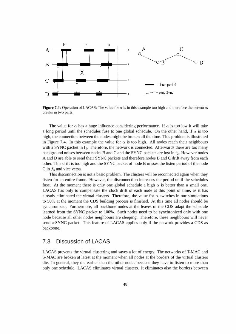
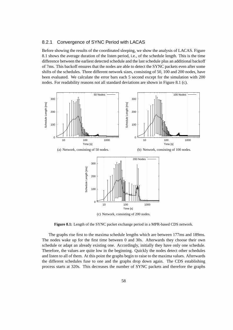
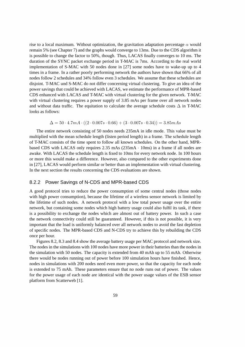
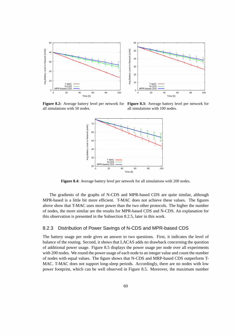
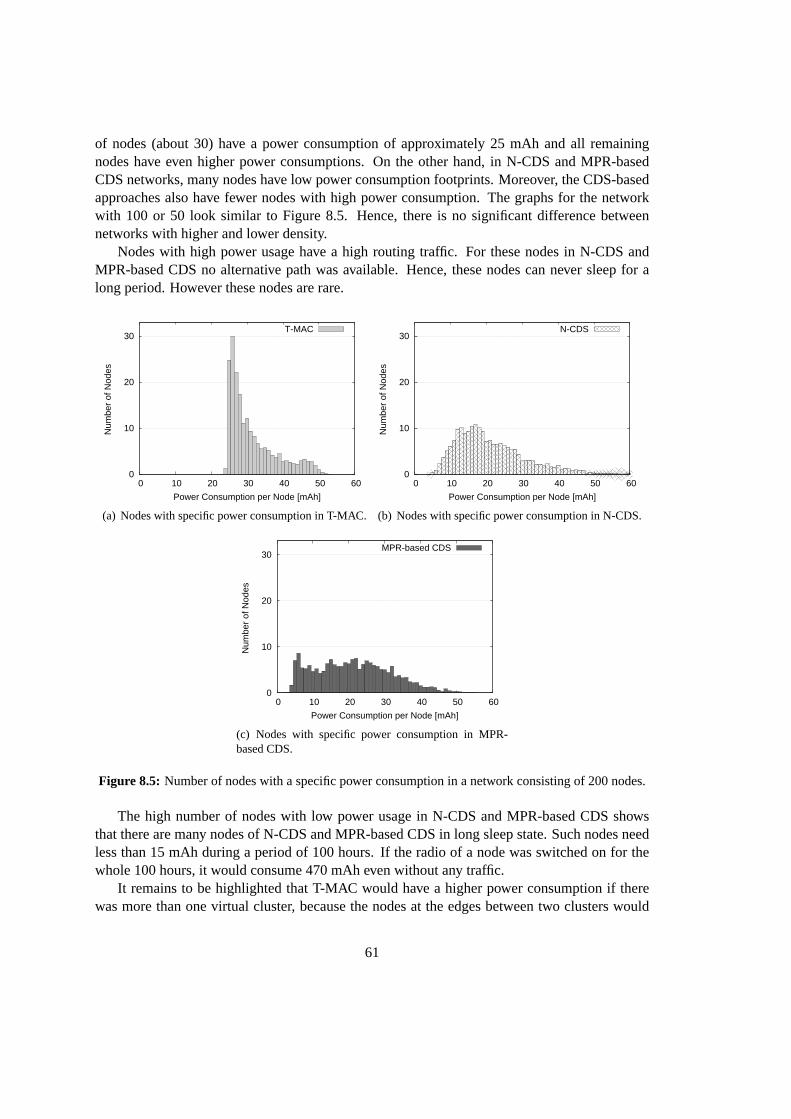
B ACKBONE CONSTRUCTION BASED ON SYNC-M ESSAGES AND ENERGY SAVINGS IN W IRELESS S ENSOR N ETWORKS Master Thesis der Philosophisch-naturwissenschaftlichen Fakult¨ at der Universit ¨ at Bern vorgelegt von Reto Zurbuchen 2009 Leiter der Arbeit: Professor Dr. Torsten Braun Institut f ¨ ur Informatik und angewandte Mathematik
In the past few years sensor networks came increasingly into scope of interest. One of themain fields of research of these kinds of networks is to save energy while running to extendthe lifetime of the battery-operated sensors. Several approaches to increase the lifetime of thebatteries of each mobile host (also called node) have been proposed. One way to save energyis to turn off the radio periodically. This can be done on theMedium Access Control (MAC)layer. Currently well known MAC protocols such asIEEE 802.11, GMS, UMTS are not energy-efficient but optimised to achieve maximum throughput. That means that there isneed for newenergy-optimised protocols in the MAC- and network layer. In this master thesis two versions ofa SYNC-message-based backbone construction mechanism for efficient MAC are presented forstatic networks. Both approaches establish a virtual backbone tree with aConnected DominatingSet (CDS). This CDS is realised without any additional packet exchange. It only adds someinformation to existing packets of a well-known sensor network protocol called T-MAC. Besidesthat, a new approach of a global synchronisation of all nodes of the network is described andevaluated. The focus is on static networks.
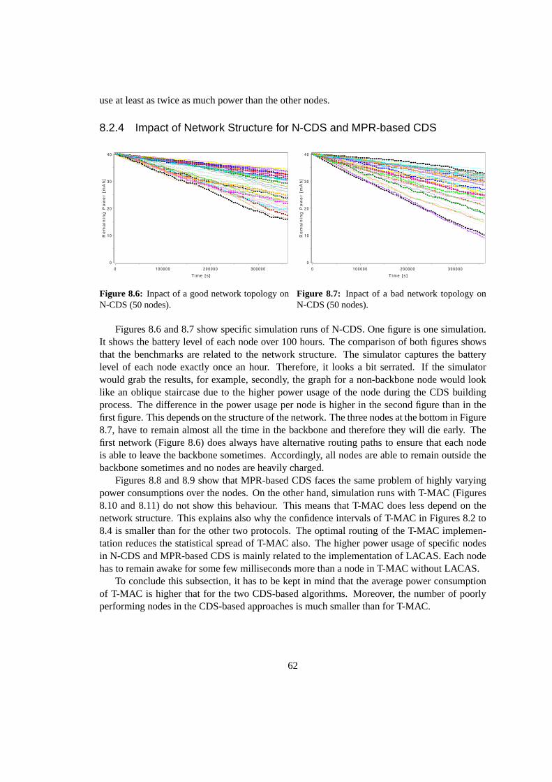
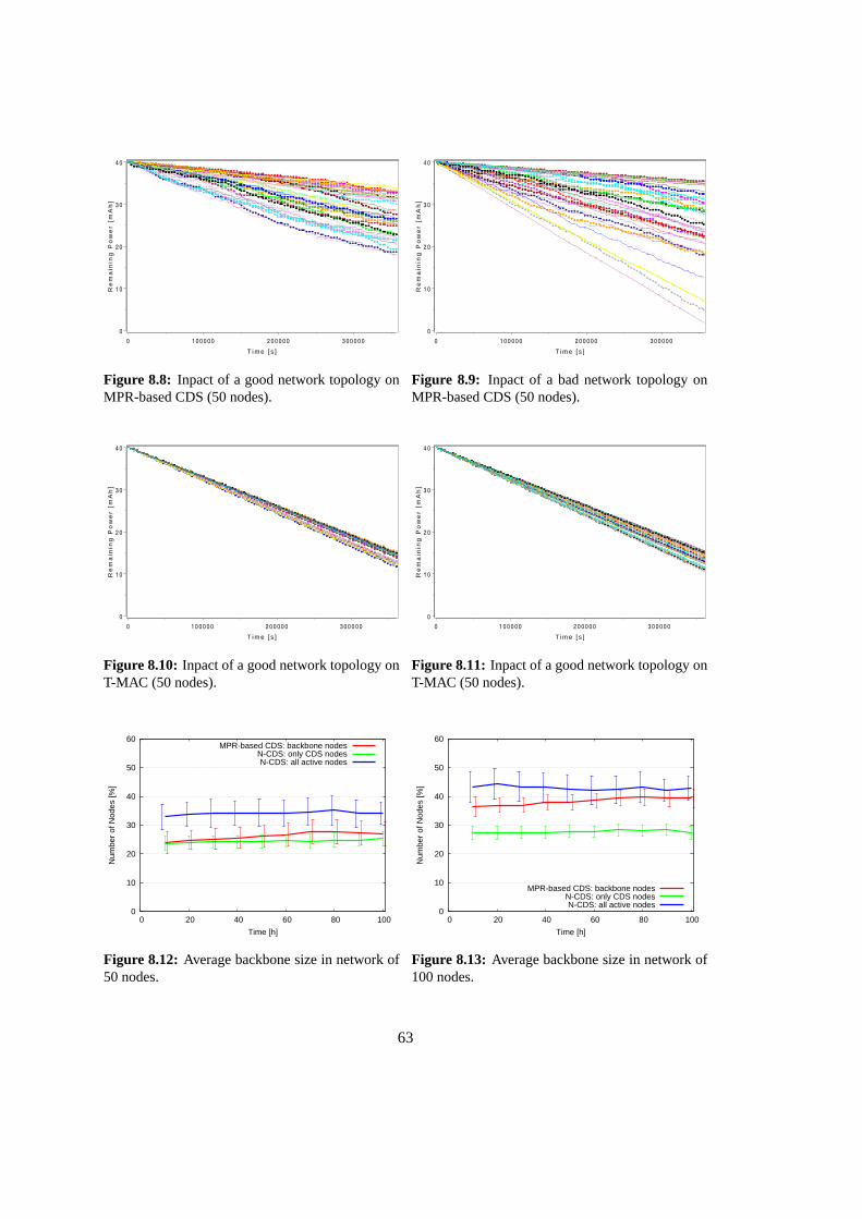
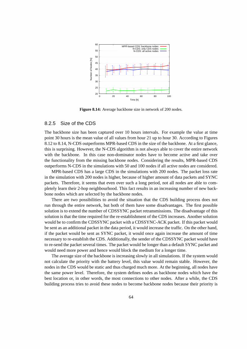
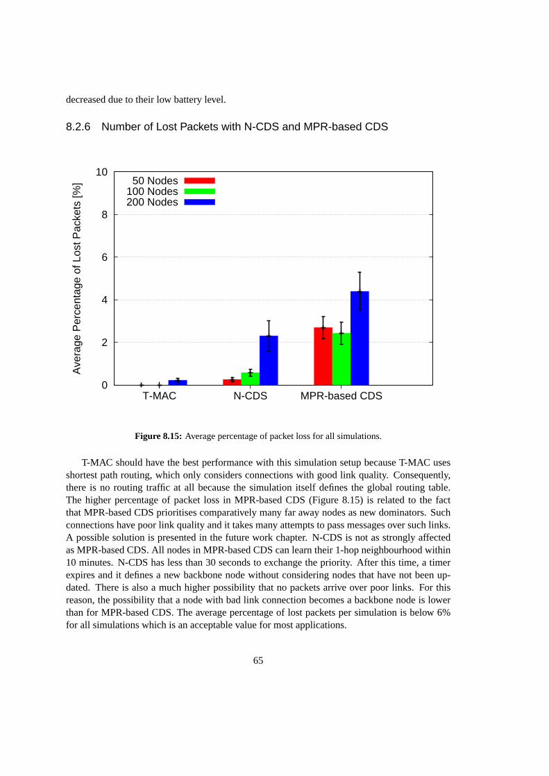
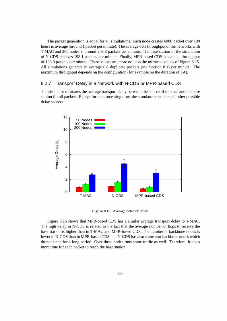
8.2 Simulation Results . . . . . . . . . . . . . . . . . . . . . . . . . . . . . . . . 578.2.1 Convergence of SYNC Period with LACAS . . . . . . . . . . . . . . . 588.2.2 Power Savings of N-CDS and MPR-based CDS . . . . . . . . . . . . . 598.2.3 Distribution of Power Savings of N-CDS and MPR-based CDS . . . . 608.2.4 Impact of Network Structure for N-CDS and MPR-based CDS . . . . .628.2.5 Size of the CDS . . . . . . . . . . . . . . . . . . . . . . . . . . . . . . 648.2.6 Number of Lost Packets with N-CDS and MPR-based CDS . . . . . . 658.2.7 Transport Delay in a Network with N-CDS or MPR-based CDS . . . . 66
9 Conclusions 67
10 Future Work 69
iv
Bibliography 70
v
Chapter 1
Introduction
A sensor network is a special kind of a wireless network. Sensor nodesimplement a radio,several sensors and a small processing unit. The entire node is battery operated. A high error-rate and malfunctions of some nodes are expected. Therefore, a sensor network requires highredundancy. To achieve high redundancy a high density of the networkis required. Anothereffect of a large number of deployed nodes is the need for dynamic topology control and routing.At the moment a node is deployed it should start sensing and try to establish routing tables ateach node. Otherwise, it could take too much time until a node is able to route a packet the firsttime. The lifetime of a network is limited by the battery lifetime of its nodes. Therefore,energy-saving approaches such as the ones proposed in this thesis are required. The main application ofsuch networks is environmental monitoring of a specific area.
1.1 Problem Statement
One of the main energy consumers of a sensor node is its radio. At the momentthe radio is off,the total energy usage of the node is decreasing by a factor of around 100 [1]. This factor variesdepending on the type of hardware of the node. The challenge is to find a way to temporallyturn off the radio of some nodes while keeping the entire network running. Agood techniquewill keep the maximum bandwidth high and the latency low as long as there are manydatapackets waiting for transmission. At the moment there are only a few data packets waiting fortransmission, the maximum bandwidth can be lowered. All these improvements have to be doneat the MAC and network layers of the communication protocol stack.
In this thesis the focus is on flat, unstructured and unsupervised networks. There are severalchallenges for a new communication protocol for such a wireless sensor network:
• The hardware of the node has to be cheap. Thus, the hardware is oftenof lower qualityand the accuracy of the clock is accordingly less exact, which leads to someclock drifts.To detect that a sender node and its particular receiver node are awake at the same time,they need bo be synchronized.
• Like in any other wireless network, the well-known hidden node problem has its impacton the protocol [2].
1
• The entire network needs to organise the routing and an optional time synchronizationitself. There is no master node (apart from the base station) and there is nohierarchyexcept of a possible MAC address for each node. Setting up static routingtables for allnodes is not feasible because of the large number of deployed nodes. Additionally, thedeployment of the nodes might be unsupervised.
• Like for other wireless protocols there are some variable background noises on the radio.There is no guarantee that a packet arrives at the destination even if there is no concurrentcommunication.
1.2 Contributions
The main contributions of our work are:
• Medium access has been optimized by exploiting the information distributed throughSYNC messages. The information has been used to achieve local synchronization andto implement routing on the MAC layer.
• A simple synchronization method for SYNC-based MAC protocols has been developed.The method prevents the existence of multiple schedules without introducing additionalcontrol traffic.
• The common schedule is realized by a gravitation-like principle, where temporary presentclusters attract each other until they fuse. Due to the usage of SYNC messages, the fusionprocess is very robust. No temporary storage of multiple schedules is necessary.
• Virtual routing backbones have been established on the MAC layer. This enables therouting over this virtual backbone without additional routing control traffic and memoryallocation.
• The backbones support routing and allow the temporary shut-down of theradios of non-backbone nodes to preserve additional energy.
1.3 Thesis Outline
This thesis is organized as follows: Chapter 2 describes existing protocolsfor wireless sensornetworks. After that Chapter 3 explains the idea of aConnecting Dominating Set (CDS), whichis an approach to setup a virtual backbone of a network. A virtual backbone is helpful to optimiserouting and to save energy. Chapter 4 introduces existing techniques to synchronize the clocksof sensor nodes. The simulations of the presented protocols and a reference protocol use thesimulation environment called OMNeT++ [3]. A brief overview of this tool is given in Chapter5. Based on the ideas of two existing MAC protocols and the theory of CDS, two new versionsof a SYNC-based MAC protocol are described in Chapter 6. For synchronization purpose,both protocols apply a new synchronisation concept calledLocal Adaptive Clock AssimilationScheme (LACAS) which is presented in Chapter 7. The functionality, implementation details
2
and the results of the simulations in comparison to an existing MAC protocol are described inChapter 8. Finally, Chapter 9 contains the conclusions and Chapter 10 contains a list of possiblefuture work.
3
Chapter 2
Medium Access Control Protocols (MAC)for Wireless Sensor Networks
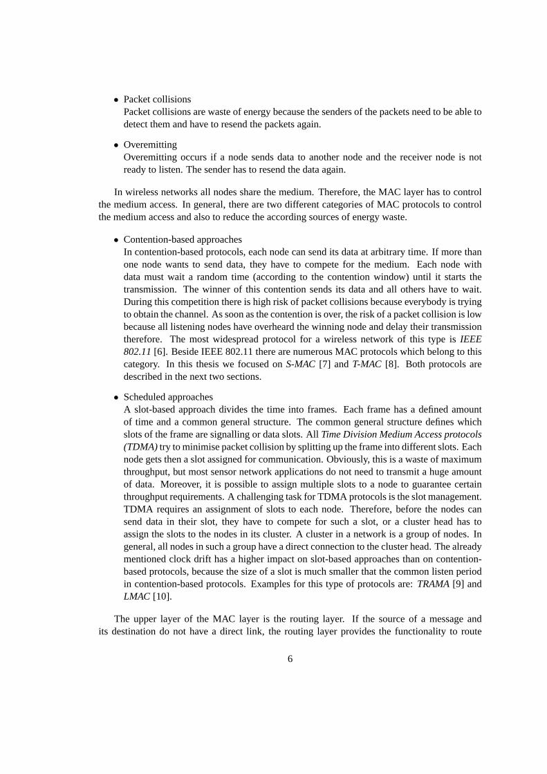
Transmitting information over a network of any kind is a challenging task. Therefore, there isa de facto standard to handle this task with several layers. Each layer is responsible for specificoperations. The lowest layer is called the physical layer. It is responsible to translate the streamof bits, which has to be transmitted, into a sequence of signals which are transmitted over thephysical connection to the destined destination. At the destination the receiver retranslates thesequence of signals back into a stream of bits and finally sends it to the upper layer called MAClayer.
The MAC layer coordinates the access to the communication medium. The main goalofclassic MAC layer protocols is to maximise the data throughput and minimise the latency. Inaddition, the MAC layer of a wireless sensor network needs to minimise the energy usage of allnodes. As mentioned in the introduction, one of the most efficient ways to save energy is to turnoff the radio periodically. On the other hand, if the radio of a specific nodeis off, there is noway to communicate with this node. Therefore, it has to be ensured that sender and receiver areawake at the same time, i.e., they need to be synchronized.
There are five major sources of energy waste in wireless sensor networks [4]. These are idlelistening, overhearing, control packet overhead, collisions and overemitting.
• Idle listeningIdle listening is the situation when a node is listening to the radio but there is no commu-nication running. Typical nodes such as the Berkeley motes [5] or the ESB(EmbeddedSensor Board) from Scatterweb [1] use in idle mode 50 - 100% of the amount of energythat is used in the receiving mode. All idle listening is huge waste of energy.
• OverhearingA node is listening to the communication on the channel but the node is not involved inthis communication. There is no need to listen to this communication.
• Control packet overheadEach transmission of data consumes energy. On the other hand, all MAC protocols needcontrol packets. Usually, an energy and maximum-bandwidth optimised MAC protocoltries to reduce the number of control packets as much as possible.
5
• Packet collisionsPacket collisions are waste of energy because the senders of the packets need to be able todetect them and have to resend the packets again.
• OveremittingOveremitting occurs if a node sends data to another node and the receivernode is notready to listen. The sender has to resend the data again.
In wireless networks all nodes share the medium. Therefore, the MAC layer has to controlthe medium access. In general, there are two different categories of MAC protocols to controlthe medium access and also to reduce the according sources of energy waste.
• Contention-based approachesIn contention-based protocols, each node can send its data at arbitrarytime. If more thanone node wants to send data, they have to compete for the medium. Each node withdata must wait a random time (according to the contention window) until it starts thetransmission. The winner of this contention sends its data and all others haveto wait.During this competition there is high risk of packet collisions because everybody is tryingto obtain the channel. As soon as the contention is over, the risk of a packetcollision is lowbecause all listening nodes have overheard the winning node and delay their transmissiontherefore. The most widespread protocol for a wireless network of thistype is IEEE802.11 [6]. Beside IEEE 802.11 there are numerous MAC protocols which belongto thiscategory. In this thesis we focused onS-MAC [7] and T-MAC [8]. Both protocols aredescribed in the next two sections.
• Scheduled approachesA slot-based approach divides the time into frames. Each frame has a defined amountof time and a common general structure. The common general structure defines whichslots of the frame are signalling or data slots. AllTime Division Medium Access protocols(TDMA) try to minimise packet collision by splitting up the frame into different slots. Eachnode gets then a slot assigned for communication. Obviously, this is a waste ofmaximumthroughput, but most sensor network applications do not need to transmit ahuge amountof data. Moreover, it is possible to assign multiple slots to a node to guarantee certainthroughput requirements. A challenging task for TDMA protocols is the slotmanagement.TDMA requires an assignment of slots to each node. Therefore, before the nodes cansend data in their slot, they have to compete for such a slot, or a cluster head has toassign the slots to the nodes in its cluster. A cluster in a network is a group of nodes. Ingeneral, all nodes in such a group have a direct connection to the clusterhead. The alreadymentioned clock drift has a higher impact on slot-based approaches than on contention-based protocols, because the size of a slot is much smaller that the common listenperiodin contention-based protocols. Examples for this type of protocols are:TRAMA [9] andLMAC [10].
The upper layer of the MAC layer is the routing layer. If the source of a message andits destination do not have a direct link, the routing layer provides the functionality to route
6
messages over intermediate nodes. The routing layer also takes care that the MAC layer knowsto which node it has to send a message.
2.1 S-MAC
2.1.1 Overview
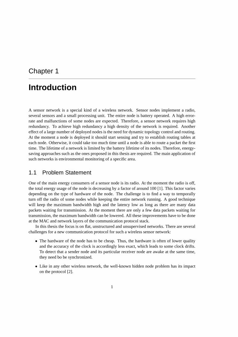
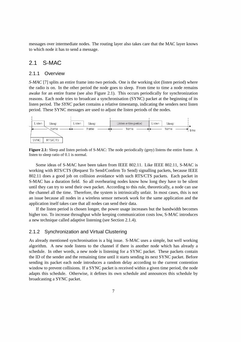
S-MAC [7] splits an entire frame into two periods. One is the working slot (listen period) wherethe radio is on. In the other period the node goes to sleep. From time to time a noderemainsawake for an entire frame (see also Figure 2.1). This occurs periodicallyfor synchronizationreasons. Each node tries to broadcast a synchronisation (SYNC) packet at the beginning of itslisten period. TheSYNC packet contains a relative timestamp, indicating the senders next listenperiod. These SYNC messages are used to adjust the listen periods of the nodes.
Figure 2.1: Sleep and listen periods of S-MAC: The node periodically (grey) listens the entire frame. Alisten to sleep ratio of 0.1 is normal.
Some ideas of S-MAC have been taken from IEEE 802.11. Like IEEE 802.11, S-MAC isworking with RTS/CTS (Request To Send/Confirm To Send) signalling packets, because IEEE802.11 does a good job on collision avoidance with such RTS/CTS packets. Each packet inS-MAC has a duration field. So all overhearing nodes know how long theyhave to be silentuntil they can try to send their own packet. According to this rule, theoretically, a node can usethe channel all the time. Therefore, the system is intrinsically unfair. In mostcases, this is notan issue because all nodes in a wireless sensor network work for the same application and theapplication itself takes care that all nodes can send their data.
If the listen period is chosen longer, the power usage increases but the bandwidth becomeshigher too. To increase throughput while keeping communication costs low, S-MAC introducesa new technique called adaptive listening (see Section 2.1.4).
2.1.2 Synchronization and Virtual Clustering
As already mentioned synchronisation is a big issue. S-MAC uses a simple, but well workingalgorithm. A new node listens to the channel if there is another node which hasalready aschedule. In other words, a new node is listening for a SYNC packet. These packets containthe ID of the sender and the remaining time until it starts sending its next SYNC packet. Beforesending its packet each node introduces a random delay according to thecurrent contentionwindow to prevent collisions. If a SYNC packet is received within a giventime period, the nodeadapts this schedule. Otherwise, it defines its own schedule and announces this schedule bybroadcasting a SYNC packet.
7
All nodes sharing the same schedule build a virtual cluster. All nodes regularly stay awakefor an entire frame. Thus they have the possibility to detect other virtual clusters. If there aretwo or more schedules from two or more nodes, the overhearing node adapts all schedules, butsends its SYNC packet only in one listen period. It still belongs to its original virtual cluster butit awakes also in the other listen periods. This means that the node has a significantly higherpower usage. Otherwise it would not be possible to send data from one virtual cluster to another.
The clock drift of each node does not affect S-MAC much, because the listen period is sig-nificantly longer than the clock drift rates. Moreover, each SYNC packet updates and adjuststhe schedules of all receivers. Therefore, nodes overhear the SYNC packets from their neigh-bourhood nodes. No SYNC packet are received in case of packet collision, if background noisesare too high, or if a node sends its SYNC packet outside the listen period duea high clock driftcaused by a high packet loss rate.
2.1.3 Overhearing Avoidance
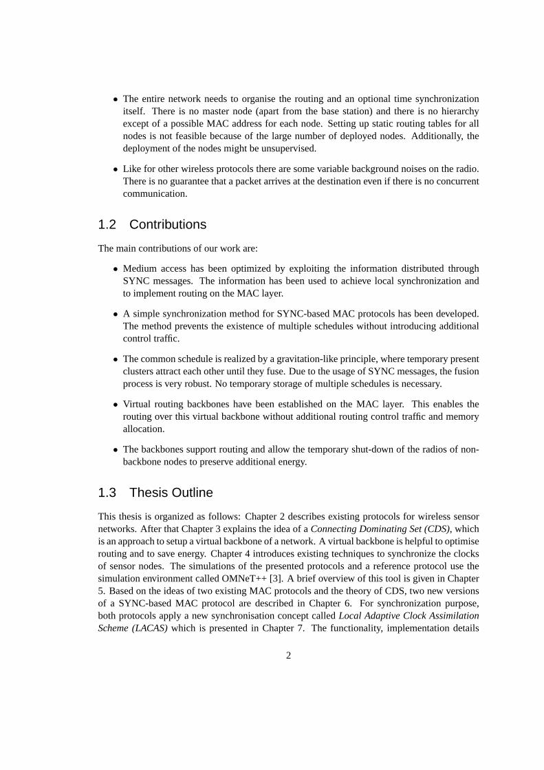
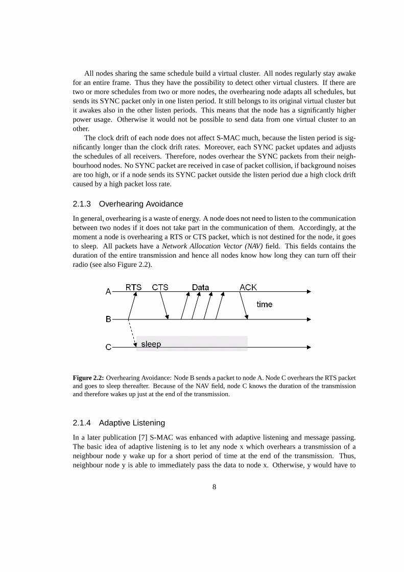
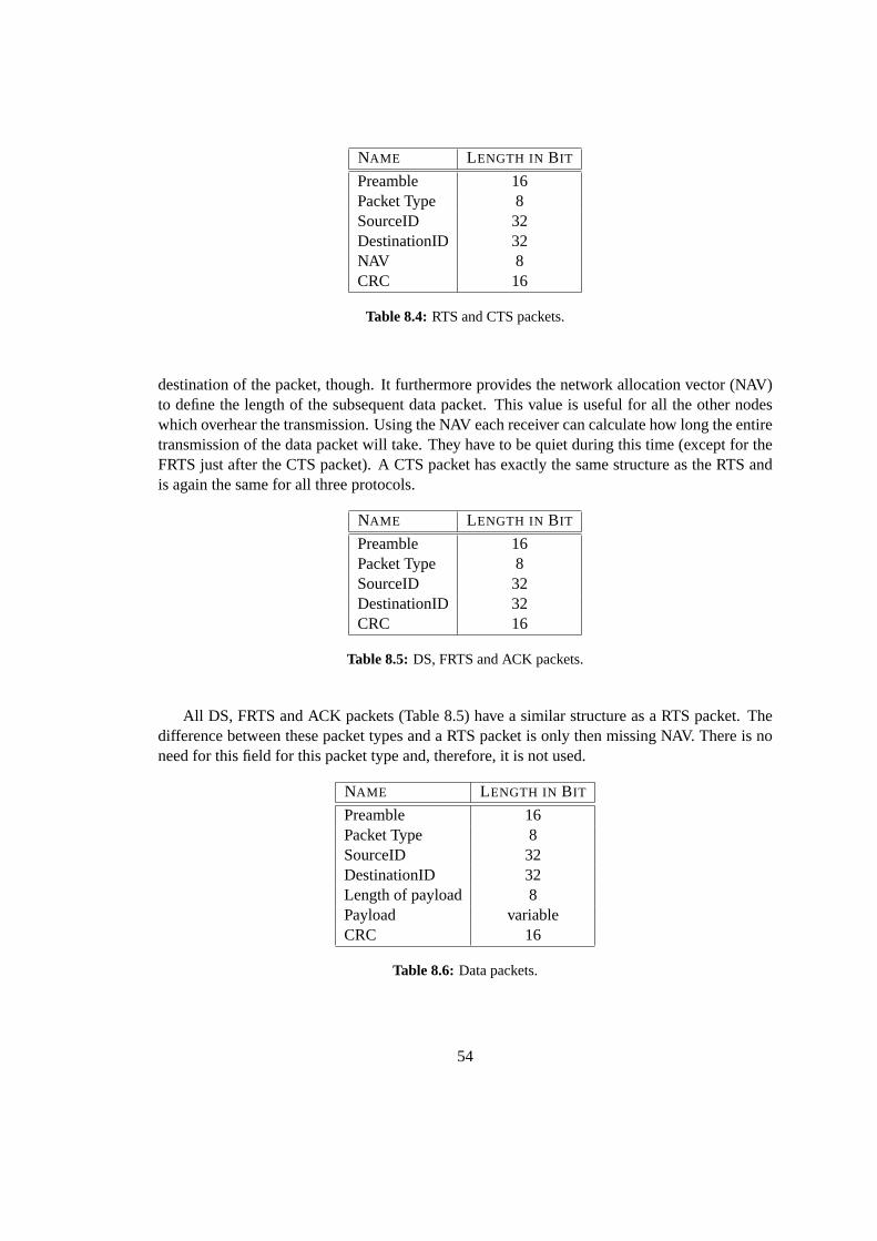
In general, overhearing is a waste of energy. A node does not need tolisten to the communicationbetween two nodes if it does not take part in the communication of them. Accordingly, at themoment a node is overhearing a RTS or CTS packet, which is not destined for the node, it goesto sleep. All packets have aNetwork Allocation Vector (NAV) field. This fields contains theduration of the entire transmission and hence all nodes know how long they can turn off theirradio (see also Figure 2.2).
Figure 2.2: Overhearing Avoidance: Node B sends a packet to node A. Node Coverhears the RTS packetand goes to sleep thereafter. Because of the NAV field, node C knows the duration of the transmissionand therefore wakes up just at the end of the transmission.
2.1.4 Adaptive Listening
In a later publication [7] S-MAC was enhanced with adaptive listening and message passing.The basic idea of adaptive listening is to let any node x which overhears a transmission of aneighbour node y wake up for a short period of time at the end of the transmission. Thus,neighbour node y is able to immediately pass the data to node x. Otherwise, y would have to
8
wait for the next scheduled listen time. If node x does not receive anything during adaptivelistening, it goes back to sleep until its next scheduled listen time.
2.1.5 Message Passing
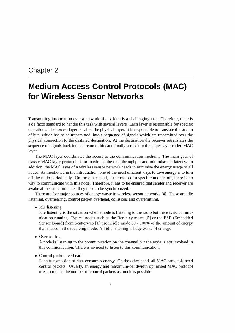
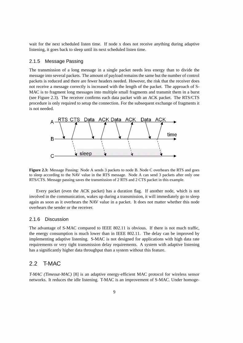
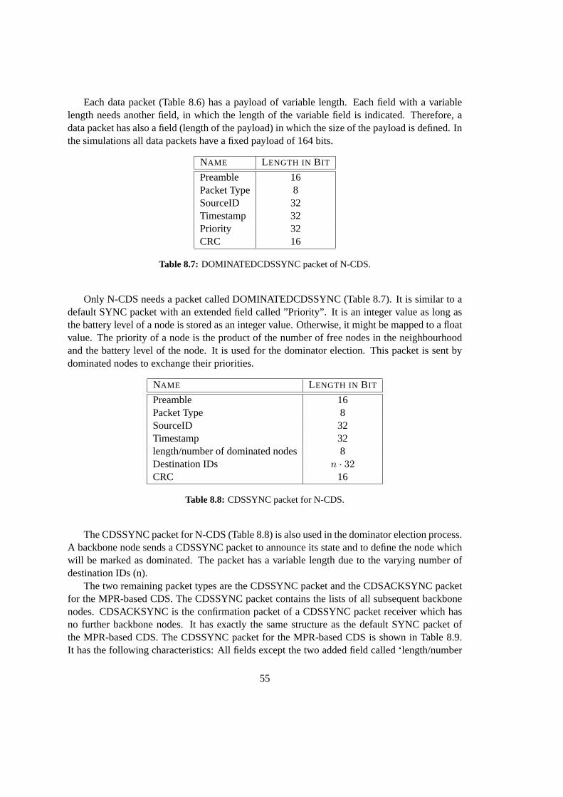
The transmission of a long message in a single packet needs less energy than to divide themessage into several packets. The amount of payload remains the same butthe number of controlpackets is reduced and there are fewer headers needed. However,the risk that the receiver doesnot receive a message correctly is increased with the length of the packet.The approach of S-MAC is to fragment long messages into multiple small fragments and transmit them in a burst(see Figure 2.3). The receiver confirms each data packet with an ACK packet. The RTS/CTSprocedure is only required to setup the connection. For the subsequentexchange of fragments itis not needed.
Figure 2.3: Message Passing: Node A sends 3 packets to node B. Node C overhears the RTS and goesto sleep according to the NAV value in the RTS message. Node A can send 3 packets after only oneRTS/CTS. Message passing saves the transmission of 2 RTS and2 CTS packet in this example.
Every packet (even the ACK packet) has a duration flag. If another node, which is notinvolved in the communication, wakes up during a transmission, it will immediately go tosleepagain as soon as it overhears the NAV value in a packet. It does not matterwhether this nodeoverhears the sender or the receiver.
2.1.6 Discussion
The advantage of S-MAC compared to IEEE 802.11 is obvious. If there is not much traffic,the energy consumption is much lower than in IEEE 802.11. The delay can be improved byimplementing adaptive listening. S-MAC is not designed for applications with highdata raterequirements or very tight transmission delay requirements. A system with adaptive listeninghas a significantly higher data throughput than a system without this feature.
2.2 T-MAC
T-MAC (Timeout-MAC) [8] is an adaptive energy-efficient MAC protocol for wireless sensornetworks. It reduces the idle listening. T-MAC is an improvement of S-MAC.Under homoge-
9
neous load both protocols achieve similar results. In a scenario with variableload, such as anevent detection application, T-MAC outperforms S-MAC, according to the authors, by a factorof up to 5. T-MAC uses the same clustering and synchronization algorithm asS-MAC (virtualclustering) [7][8]. The main difference between T-MAC and S-MAC is theidea of a variablelength of the listen period. If there is no data to be sent, the listen period can beshortened. Eachnode can switch to sleep mode at the moment it determines that there is currently no traffic forit. On the other hand, a node in T-MAC never goes to sleep as long as any communication isoverheard. It always remains awake until the end of the transmission. There is consequently nooverhearing avoidance like in S-MAC.
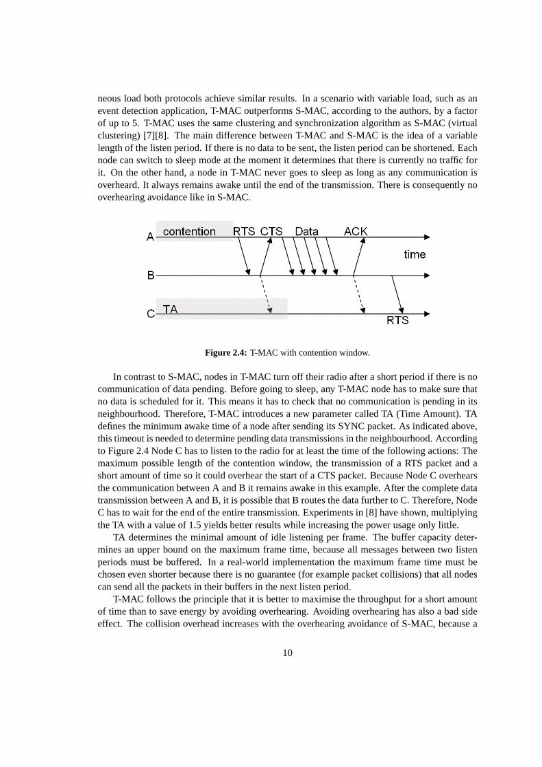
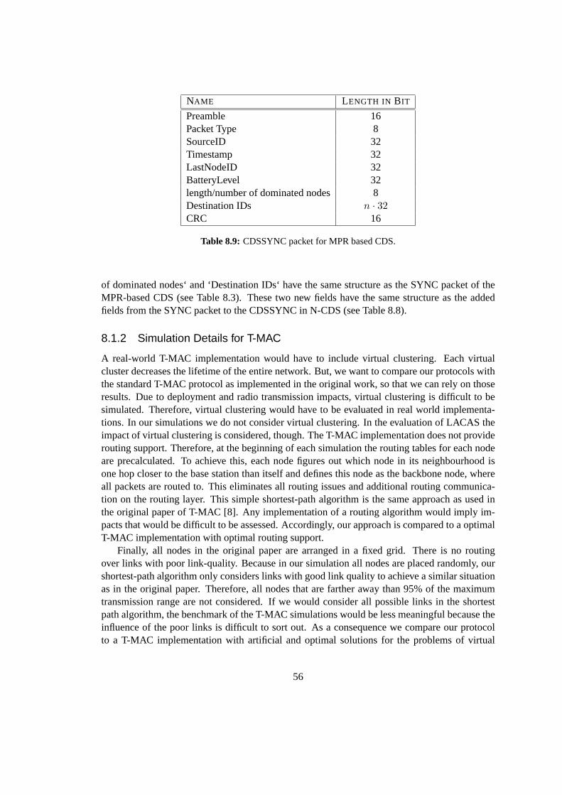
Figure 2.4: T-MAC with contention window.
In contrast to S-MAC, nodes in T-MAC turn off their radio after a short period if there is nocommunication of data pending. Before going to sleep, any T-MAC node hasto make sure thatno data is scheduled for it. This means it has to check that no communication is pending in itsneighbourhood. Therefore, T-MAC introduces a new parameter calledTA (Time Amount). TAdefines the minimum awake time of a node after sending its SYNC packet. As indicated above,this timeout is needed to determine pending data transmissions in the neighbourhood. Accordingto Figure 2.4 Node C has to listen to the radio for at least the time of the following actions: Themaximum possible length of the contention window, the transmission of a RTS packet and ashort amount of time so it could overhear the start of a CTS packet. Because Node C overhearsthe communication between A and B it remains awake in this example. After the complete datatransmission between A and B, it is possible that B routes the data further to C.Therefore, NodeC has to wait for the end of the entire transmission. Experiments in [8] have shown, multiplyingthe TA with a value of 1.5 yields better results while increasing the power usageonly little.
TA determines the minimal amount of idle listening per frame. The buffer capacitydeter-mines an upper bound on the maximum frame time, because all messages betweentwo listenperiods must be buffered. In a real-world implementation the maximum frame time must bechosen even shorter because there is no guarantee (for example packet collisions) that all nodescan send all the packets in their buffers in the next listen period.
T-MAC follows the principle that it is better to maximise the throughput for a short amountof time than to save energy by avoiding overhearing. Avoiding overhearing has also a bad sideeffect. The collision overhead increases with the overhearing avoidance of S-MAC, because a
10
node which is not involved in a communication could disturb some communication by sendinga RTS packet after awaking. This cannot be prevented because of thecommunication model ofS-MAC.
2.2.1 Early Sleeping Problem
A node can go to sleep at the moment there are no more packets to be transmitted toit. However,it is difficult for a node to determine whether there is a transmission waiting for itor not. A nodedoes not always know if another node wants to send data to it and therefore it might turn off itsradio too early. This early sleeping problem forces T-MAC to have a different data exchangemechanism than S-MAC. The problem is discussed in the following.
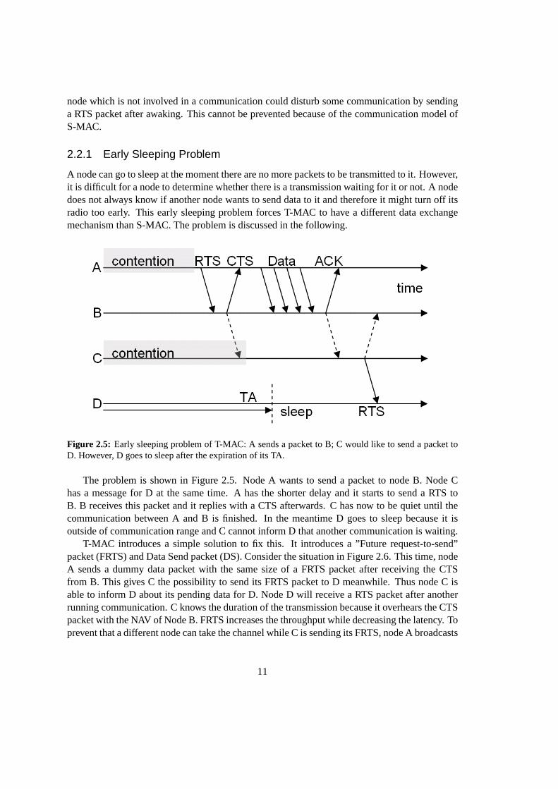
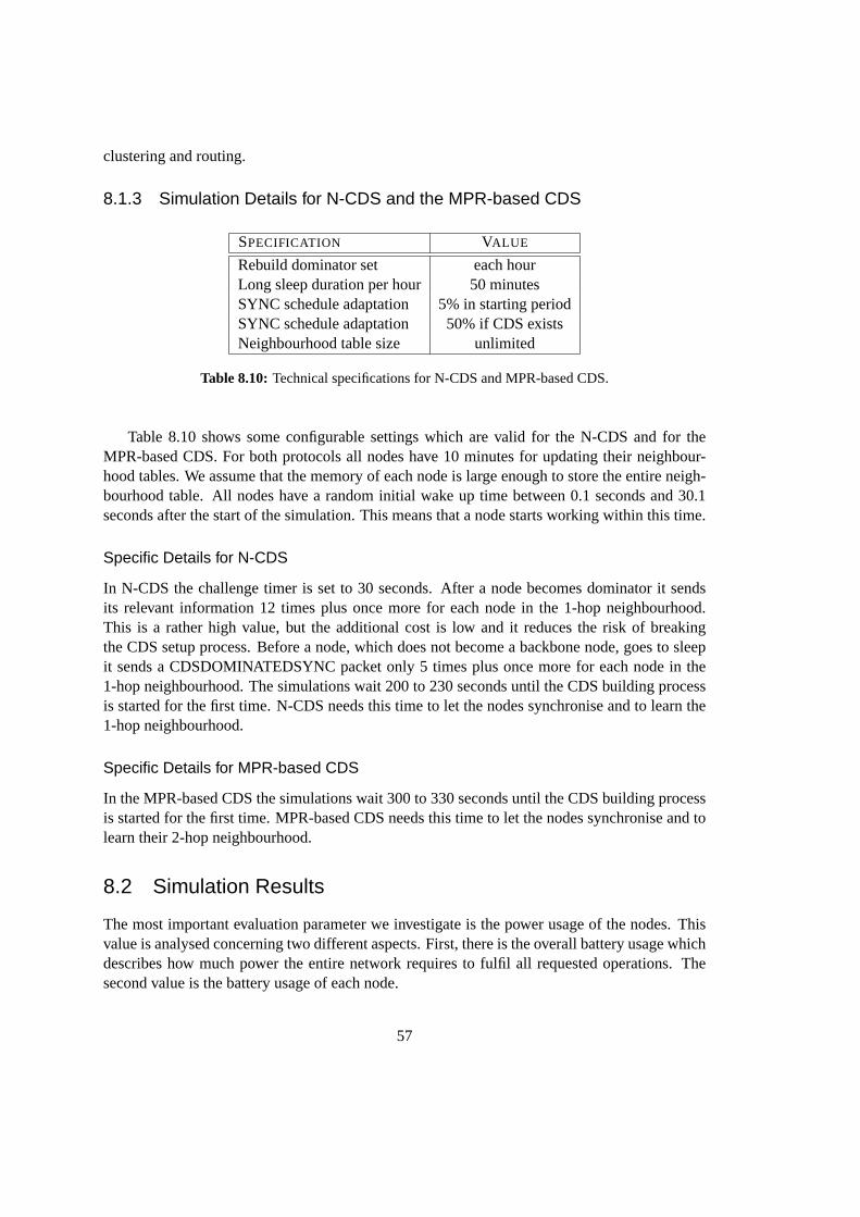
Figure 2.5: Early sleeping problem of T-MAC: A sends a packet to B; C wouldlike to send a packet toD. However, D goes to sleep after the expiration of its TA.
The problem is shown in Figure 2.5. Node A wants to send a packet to node B. Node Chas a message for D at the same time. A has the shorter delay and it starts to send a RTS toB. B receives this packet and it replies with a CTS afterwards. C has nowto be quiet until thecommunication between A and B is finished. In the meantime D goes to sleep because it isoutside of communication range and C cannot inform D that another communication is waiting.
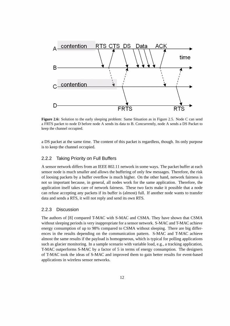
T-MAC introduces a simple solution to fix this. It introduces a ”Future request-to-send”packet (FRTS) and Data Send packet (DS). Consider the situation in Figure 2.6. This time, nodeA sends a dummy data packet with the same size of a FRTS packet after receiving the CTSfrom B. This gives C the possibility to send its FRTS packet to D meanwhile. Thus node C isable to inform D about its pending data for D. Node D will receive a RTS packet after anotherrunning communication. C knows the duration of the transmission because it overhears the CTSpacket with the NAV of Node B. FRTS increases the throughput while decreasing the latency. Toprevent that a different node can take the channel while C is sending its FRTS, node A broadcasts
11
Figure 2.6: Solution to the early sleeping problem: Same Situation as inFigure 2.5. Node C can senda FRTS packet to node D before node A sends its data to B. Concurrently, node A sends a DS Packet tokeep the channel occupied.
a DS packet at the same time. The content of this packet is regardless, though. Its only purposeis to keep the channel occupied.
2.2.2 Taking Priority on Full Buffers
A sensor network differs from an IEEE 802.11 network in some ways. The packet buffer at eachsensor node is much smaller and allows the buffering of only few messages.Therefore, the riskof loosing packets by a buffer overflow is much higher. On the other hand, network fairness isnot so important because, in general, all nodes work for the same application. Therefore, theapplication itself takes care of network fairness. These two facts make it possible that a nodecan refuse accepting any packets if its buffer is (almost) full. If another node wants to transferdata and sends a RTS, it will not reply and send its own RTS.
2.2.3 Discussion
The authors of [8] compared T-MAC with S-MAC and CSMA. They have shown that CSMAwithout sleeping periods is very inappropriate for a sensor network. S-MAC and T-MAC achieveenergy consumption of up to 98% compared to CSMA without sleeping. Thereare big differ-ences in the results depending on the communication pattern. S-MAC and T-MAC achievealmost the same results if the payload is homogeneous, which is typical for polling applicationssuch as glacier monitoring. In a sample scenario with variable load, e.g., a tracking application,T-MAC outperforms S-MAC by a factor of 5 in terms of energy consumption.The designersof T-MAC took the ideas of S-MAC and improved them to gain better results forevent-basedapplications in wireless sensor networks.
12
Chapter 3
Connected Dominating Sets (CDS)
3.1 Introduction
There are already some papers and works about establishing and running a Connected Dominat-ing Set (CDS), but only few of them focus on wireless sensor networks[11]. Moreover, mostof the published papers use the CDS for routing purpose [11],[12],[13]. Only few introduce theCDS to save energy. One could say that a CDS is a kind of a virtual backbone in a wirelessnetwork. A CDS is defined as follows (taken from [12]): ”In general, adominating set (DS) ofa graph G = (V,E) is a subset V’⊂ V such that each node in V - V’ is adjacent to some node inV’, and a connected dominating set (CDS) is a dominating set which also induces a connectedsubgraph of G. A (connected) dominating set of a wireless ad hoc network is a (connected) dom-inating set of the corresponding unit-disk graph. To simplify the connectivity management, it isdesirable to find a minimum connected dominating set (MCDS) of a given set ofnodes.”
Finding a MCDS is NP-complete, though. Therefore, heuristics are used toapproximatea MCDS. In this chapter three relevant approaches are introduced. Our own approach is thenpresented in Chapter 6.
Figure 3.1: CDS and MCDS
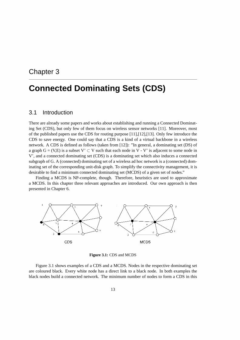
Figure 3.1 shows examples of a CDS and a MCDS. Nodes in the respective dominating setare coloured black. Every white node has a direct link to a black node. Inboth examples theblack nodes build a connected network. The minimum number of nodes to forma CDS in this
13
example is two. Therefore, the CDS on the right is a MCDS.
3.2 CDS with Pruning Rules
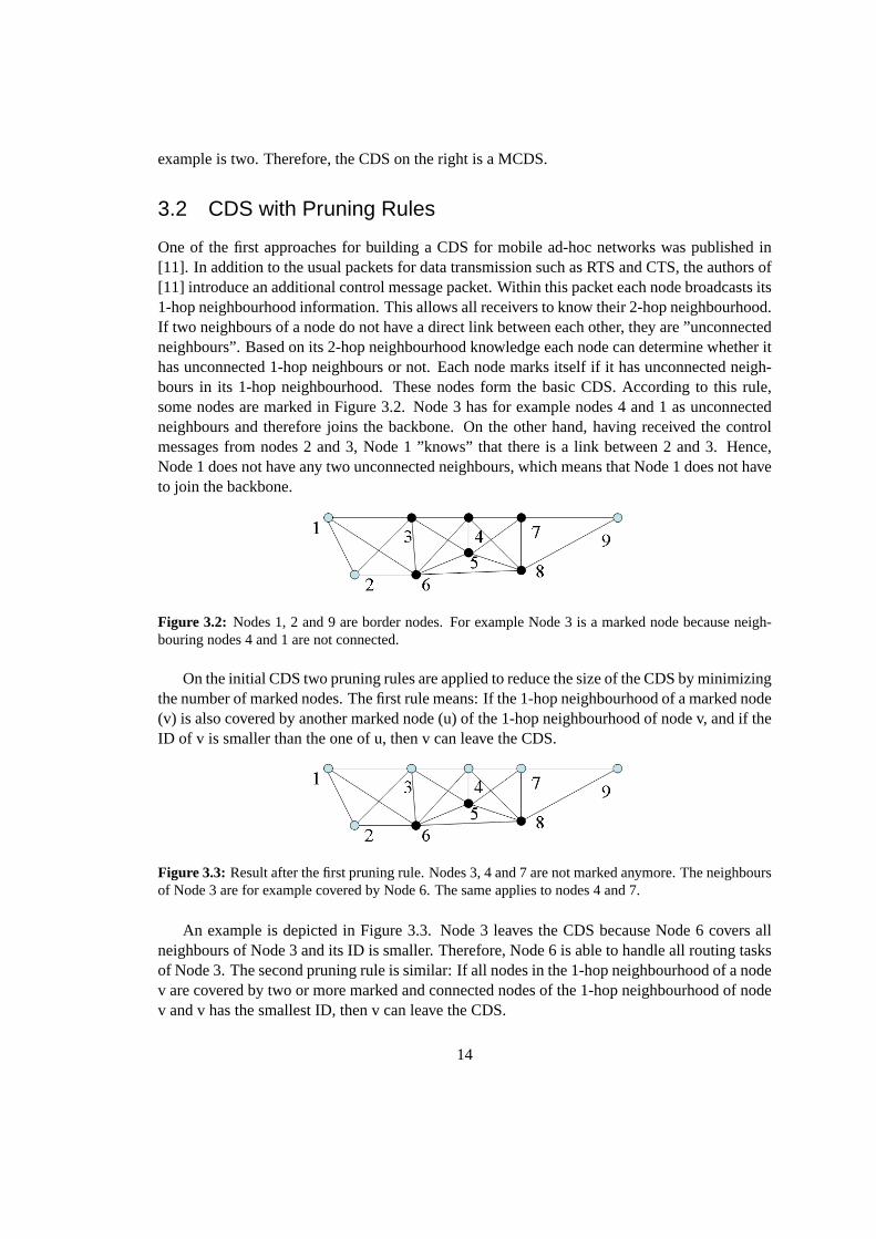
One of the first approaches for building a CDS for mobile ad-hoc networks was published in[11]. In addition to the usual packets for data transmission such as RTS and CTS, the authors of[11] introduce an additional control message packet. Within this packet each node broadcasts its1-hop neighbourhood information. This allows all receivers to know their2-hop neighbourhood.If two neighbours of a node do not have a direct link between each other, they are ”unconnectedneighbours”. Based on its 2-hop neighbourhood knowledge each node can determine whether ithas unconnected 1-hop neighbours or not. Each node marks itself if it has unconnected neigh-bours in its 1-hop neighbourhood. These nodes form the basic CDS. According to this rule,some nodes are marked in Figure 3.2. Node 3 has for example nodes 4 and 1as unconnectedneighbours and therefore joins the backbone. On the other hand, having received the controlmessages from nodes 2 and 3, Node 1 ”knows” that there is a link between2 and 3. Hence,Node 1 does not have any two unconnected neighbours, which means that Node 1 does not haveto join the backbone.
Figure 3.2: Nodes 1, 2 and 9 are border nodes. For example Node 3 is a markednode because neigh-bouring nodes 4 and 1 are not connected.
On the initial CDS two pruning rules are applied to reduce the size of the CDS byminimizingthe number of marked nodes. The first rule means: If the 1-hop neighbourhood of a marked node(v) is also covered by another marked node (u) of the 1-hop neighbourhood of node v, and if theID of v is smaller than the one of u, then v can leave the CDS.
Figure 3.3: Result after the first pruning rule. Nodes 3, 4 and 7 are not marked anymore. The neighboursof Node 3 are for example covered by Node 6. The same applies tonodes 4 and 7.
An example is depicted in Figure 3.3. Node 3 leaves the CDS because Node 6 covers allneighbours of Node 3 and its ID is smaller. Therefore, Node 6 is able to handle all routing tasksof Node 3. The second pruning rule is similar: If all nodes in the 1-hop neighbourhood of a nodev are covered by two or more marked and connected nodes of the 1-hop neighbourhood of nodev and v has the smallest ID, then v can leave the CDS.
14
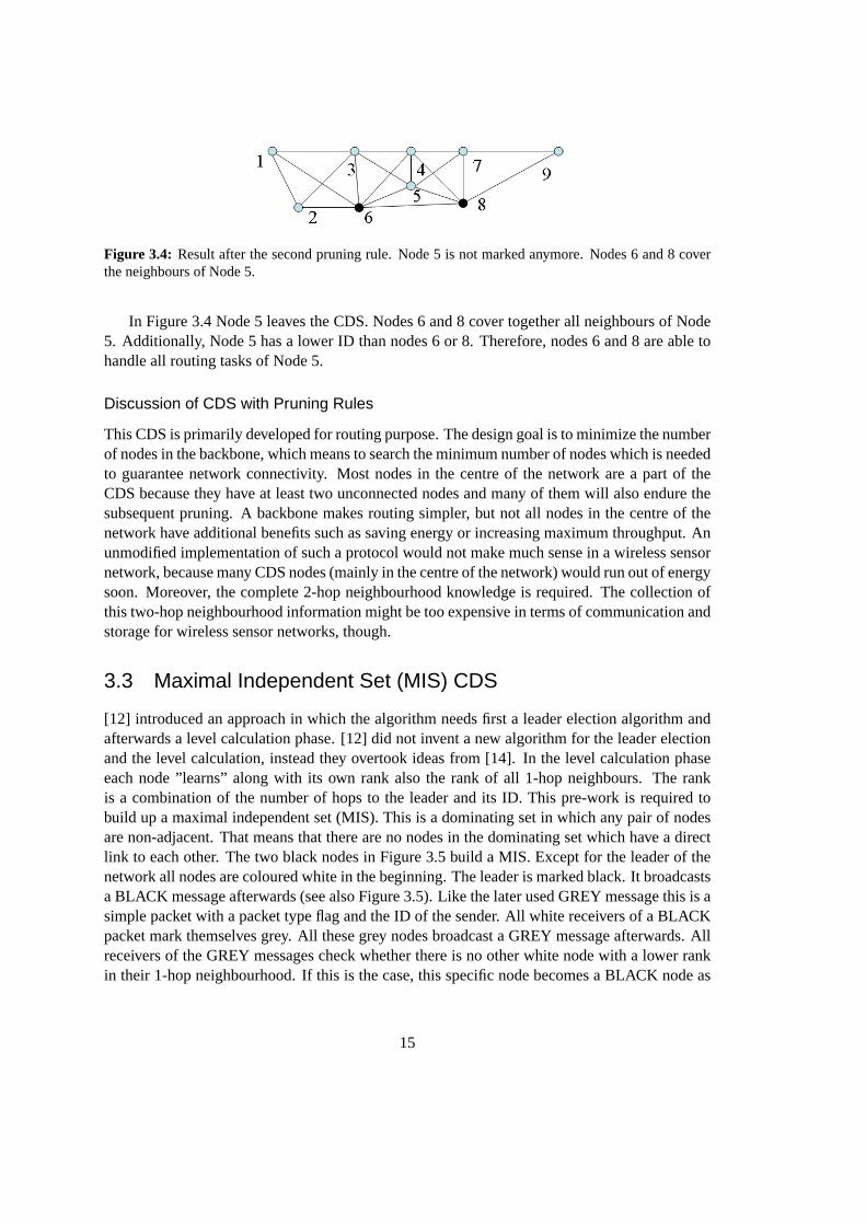
Figure 3.4: Result after the second pruning rule. Node 5 is not marked anymore. Nodes 6 and 8 coverthe neighbours of Node 5.
In Figure 3.4 Node 5 leaves the CDS. Nodes 6 and 8 cover together all neighbours of Node5. Additionally, Node 5 has a lower ID than nodes 6 or 8. Therefore, nodes 6 and 8 are able tohandle all routing tasks of Node 5.
Discussion of CDS with Pruning Rules
This CDS is primarily developed for routing purpose. The design goal is to minimize the numberof nodes in the backbone, which means to search the minimum number of nodeswhich is neededto guarantee network connectivity. Most nodes in the centre of the network are a part of theCDS because they have at least two unconnected nodes and many of themwill also endure thesubsequent pruning. A backbone makes routing simpler, but not all nodes in the centre of thenetwork have additional benefits such as saving energy or increasing maximum throughput. Anunmodified implementation of such a protocol would not make much sense in a wireless sensornetwork, because many CDS nodes (mainly in the centre of the network) would run out of energysoon. Moreover, the complete 2-hop neighbourhood knowledge is required. The collection ofthis two-hop neighbourhood information might be too expensive in terms of communication andstorage for wireless sensor networks, though.
3.3 Maximal Independent Set (MIS) CDS
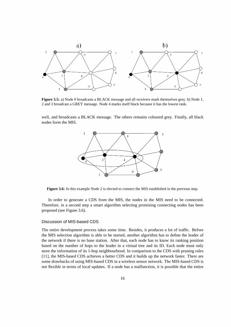
[12] introduced an approach in which the algorithm needs first a leader election algorithm andafterwards a level calculation phase. [12] did not invent a new algorithmfor the leader electionand the level calculation, instead they overtook ideas from [14]. In the level calculation phaseeach node ”learns” along with its own rank also the rank of all 1-hop neighbours. The rankis a combination of the number of hops to the leader and its ID. This pre-work isrequired tobuild up a maximal independent set (MIS). This is a dominating set in which anypair of nodesare non-adjacent. That means that there are no nodes in the dominating setwhich have a directlink to each other. The two black nodes in Figure 3.5 build a MIS. Except forthe leader of thenetwork all nodes are coloured white in the beginning. The leader is markedblack. It broadcastsa BLACK message afterwards (see also Figure 3.5). Like the later used GREY message this is asimple packet with a packet type flag and the ID of the sender. All white receivers of a BLACKpacket mark themselves grey. All these grey nodes broadcast a GREY message afterwards. Allreceivers of the GREY messages check whether there is no other white node with a lower rankin their 1-hop neighbourhood. If this is the case, this specific node becomes a BLACK node as
15
Figure 3.5: a) Node 0 broadcasts a BLACK message and all receivers mark themselves grey. b) Node 1,2 and 3 broadcast a GREY message. Node 4 marks itself black because it has the lowest rank.
well, and broadcasts a BLACK message. The others remains coloured grey. Finally, all blacknodes form the MIS.
Figure 3.6: In this example Node 2 is elected to connect the MIS established in the previous step.
In order to generate a CDS from the MIS, the nodes in the MIS need to be connected.Therefore, in a second step a smart algorithm selecting promising connecting nodes has beenproposed (see Figure 3.6).
Discussion of MIS-based CDS
The entire development process takes some time. Besides, it produces a lotof traffic. Beforethe MIS selection algorithm is able to be started, another algorithm has to definethe leader ofthe network if there is no base station. After that, each node has to know its ranking positionbased on the number of hops to the leader in a virtual tree and its ID. Each node must onlystore the information of its 1-hop neighbourhood. In comparison to the CDS with pruning rules[11], the MIS-based CDS achieves a better CDS and it builds up the network faster. There aresome drawbacks of using MIS-based CDS in a wireless sensor network.The MIS-based CDS isnot flexible in terms of local updates. If a node has a malfunction, it is possible that the entire
16
process needs to be restarted. Last but not least, the algorithm with its different algorithmic stepsmight be too time consuming to be implemented on a wireless sensor node.
3.4 Timer-based CDS
The MAC-Layer Timer-based Connected Dominating Set Construction Protocol (MTCDS) hasbeen introduced in [15]. This protocol aims at saving energy and enabling routing in general.The protocol is divided into two parts. The first one is called the initiator election. Duringthis phase, it defines the initiating node or initiator of the second phase. If a base station isthe initiator, this phase can be skipped. MTCDS uses the node ID and determines the nodewith the smallest ID as initiator. In the second phase, the initiator starts to construct the CDS.For this, the initiator becomes a member of the CDS (inDS) and announces this in the beaconframe extension of a normal IEEE 802.11 beacon message. A node periodically broadcasts thesebeacons, which are similar to the SYNC packets in S-MAC or T-MAC. The beacon contains theID of the sender. From beacon messages, each node is able to learn its 1-hop neighbourhood. Itsextension has a size of 58 bits. This is only about 10% of the default beacon packet size of IEEE802.11, which is about 550 bits. The beacon extension contains the status of the node, which iseither uncovered, covered or in DS. The initial state is uncovered. All receivers of the beaconsent by the initiator become covered nodes, which means that they have a 1-hop connection tothe CDS. All receivers start a timer immediately. The value of this timer is defined for all nodeswith one or more uncovered neighbours by the following function:
∆T = Tmax ·1
(number of uncovered neighbours)α(3.1)
When the timer expires, the node becomes a member of the CDS and announcesthis in thenext beacon frame extension. If the number of uncovered neighboursis 0, the specific node isnot part of the CDS.
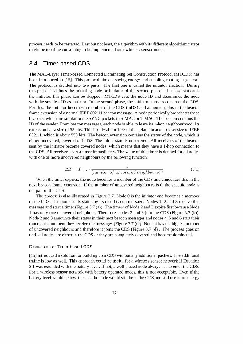
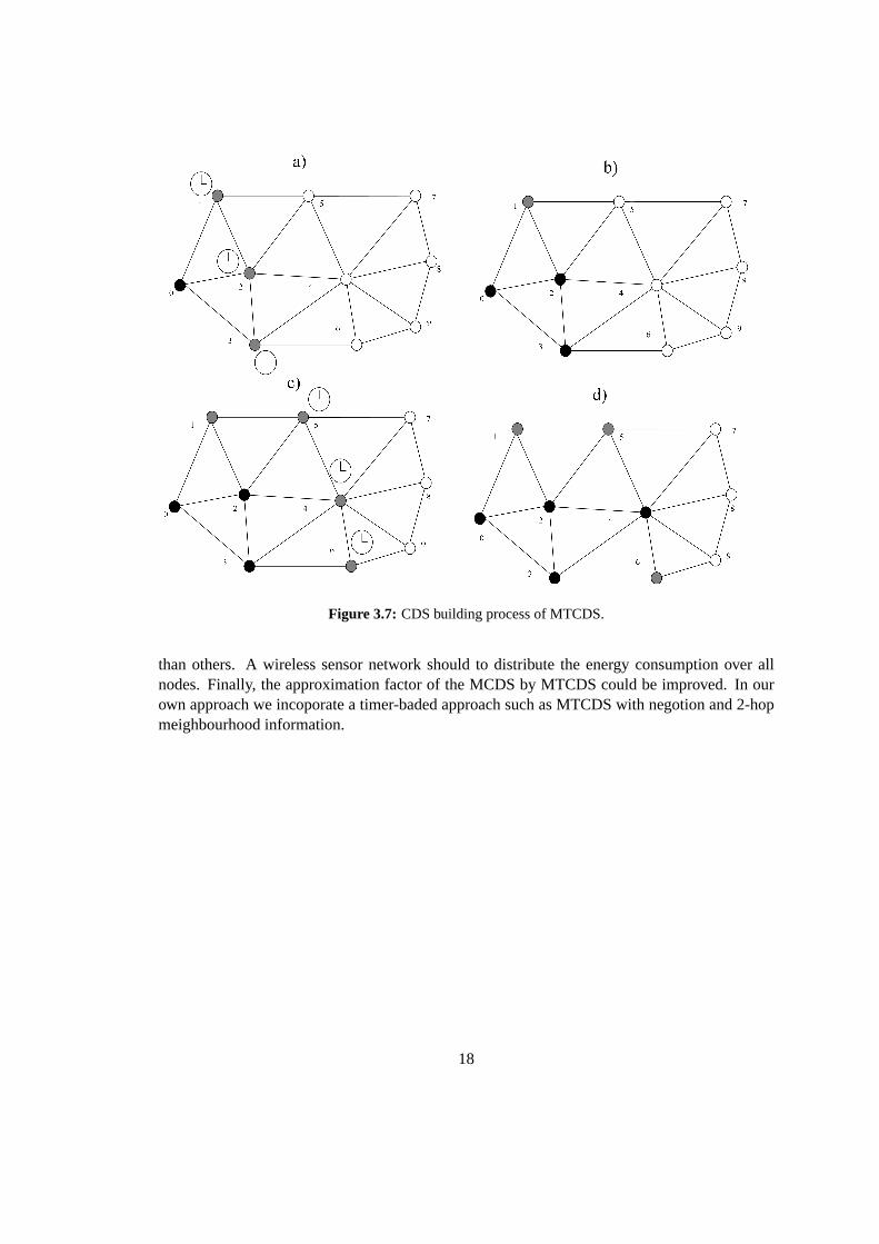
The process is also illustrated in Figure 3.7. Node 0 is the initiator and becomes amemberof the CDS. It announces its status by its next beacon message. Nodes 1,2 and 3 receive thismessage and start a timer (Figure 3.7 (a)). The timers of Node 2 and 3 expirefirst because Node1 has only one uncovered neighbour. Therefore, nodes 2 and 3 join the CDS (Figure 3.7 (b)).Node 2 and 3 announce their status in their next beacon messages and nodes 4, 5 and 6 start theirtimer at the moment they receive the messages (Figure 3.7 (c)). Node 4 has the highest numberof uncovered neighbours and therefore it joins the CDS (Figure 3.7 (d)). The process goes onuntil all nodes are either in the CDS or they are completely covered and become dominated.
Discussion of Timer-based CDS
[15] introduced a solution for building up a CDS without any additional packets. The additionaltraffic is low as well. This approach could be useful for a wireless sensor network if Equation3.1 was extended with the battery level. If not, a well placed node always has to enter the CDS.For a wireless sensor network with battery operated nodes, this is not acceptable. Even if thebattery level would be low, the specific node would still be in the CDS and still use more energy
17
Figure 3.7: CDS building process of MTCDS.
than others. A wireless sensor network should to distribute the energy consumption over allnodes. Finally, the approximation factor of the MCDS by MTCDS could be improved. In ourown approach we incoporate a timer-baded approach such as MTCDS withnegotion and 2-hopmeighbourhood information.
18
Chapter 4
Clock Synchronization
4.1 Introduction
Each node has an internal clock. The nodes use this clock mainly for internal alerts but theapplication itself could need the clock as well. For example, an application that detects sensorevents and sends them to the base station needs a clock. Otherwise, the base station will notknow how old this information is. On the other hand, nodes for wireless sensor networks haveto be cheap. Cheap devices are normally not as exact as expensive ones. Consequently, due tofabrication reasons each node has an individual clock drift which is not negligible. For manyMAC protocols there is the requirement that nodes are synchronized, atleast with the nodes intheir neighbourhood. In other words, many MAC protocols need a solutionto synchronize thenodes. In this chapter an overview over relevant related work is given. Our own solution is thenproposed in Chapter 7.
4.2 Network Time Protocol NTP
NTP [16] is a well-known protocol used mainly in the Internet. The first definition was madein 1992. NTP works with reference clocks. These are atomic (caesium, rubidium) clocks, GPSclocks or other radio clocks. These reference clocks are the roots ofa hierarchical system of”clock strata”. All reference clocks have, therefore, the stratum level 0. All hosts which are ableto get the time from a stratum n device will become stratum n + 1. Accordingly, a client of aNTP server acts as a server to down-link devices.
If a NTP client wants to update its clock, it sends a request packet to a NTPserver. Thispacket contains the timestamp of the client. The server adds its own timestamp and atransmittimestamp to this packet before it sends the packet back. The second timestamphelps the clientto determine the travelling time of the packet. Thus, the client can estimate the actualtime ofthe server. It is only an approximation because there are several delays. There are some variableprocessing times at the client and at the server and there is a variable transmission delay over thenetwork. The shorter and more symmetric the round-trip time is, the more accurate the estimateof the server time will be. This procedure is performed several times before it passes some sanitychecks.
19
Discussion of NTP and Wireless Sensor Networks
NTP works well but it is not optimised for energy and does not exploit a broadcast medium.Additionally, there is a lot of preconfiguration required until it works in a new, independentnetwork.
4.3 Time Synchronisation with GPS
GPS (Global Positioning System)[17] computes the position of a GPS device allover the world.Exact clock synchronization with the GPS satellites is required to achieve an accurate positionestimate. More than 24 satellites are currently placed in the orbit. Each of them knows its exactposition and the current time. Each satellite has more than one atomic clock on board.
The basic principle of GPS is simple. All satellites periodically broadcast their positionand the time of sending this information. With the time difference between sending the dataand receiving it at a receiver it is possible to estimate the distance between sender and receiver.Moreover, because the propagation speed of the signal approximates light speed, the clocks atthe receiver are adjusted very exact. In general there are 3 unknown variables. This are x andy for the position and t for time. At the moment there are at least four satellites visible, it ispossible to solve the according system of equations. With five visible satellites itis possible todetermine also the altitude.
Discussion of Time Synchronisation with GPS
GPS is an exact approach to compute the current time. There are severaldisadvantages for usingit in a wireless sensor network, though. First, the GPS module takes a lot of energy. ModernGPS receiver chips like the SIRF Star III [18] still need about 50 mW. GPSdevice needs lineof sight to contact the satellites. Without a relay GPS is not available indoors.And last but notleast, a GPS chip still costs several dollars.
4.4 IEEE 802.11 Synchronization
IEEE 802.11 defines a Timing Synchronization Function (TSF) for the ad-hoc mode in the MAClayer of a wireless network. Basically it uses a similar concept as S-MAC and T-MAC, i.e., asynchronization packet is periodically broadcast by each node. IEEE802.11 defines a frame-length. The length of this frame depends on the various IEEE 802.11 standards and bit-rates.At the beginning of each frame there is a beacon generation window. Eachnode defines at thebeginning of the first window a random number which is uniformly distributed between 0 and wwhere w is 15 or 31. This value represents the delay until it tries to send its beacon. Each beaconcontains a timestamp among other parameters. At the moment a node overhears abeacon fromanother node it will cancel its own pending beacon transmission and adjustits own clock to thetimestamp of the received beacon. TSF will never adjust a clock backwards. If the receivedtimestamp is older than the current of the receiving node, it is discarded. Thus, TSF adjusts theclocks to the fastest one in the entire network.
20
Discussion of IEEE 802.11 Synchronization
TSF is easy to implement. It never achieves such good accuracy as NTP orGPS. On the otherhand, there is no additional hardware required and the additional trafficis low. If the nodes arelistening to the radio only during the beacon generation window, it is possible that a node getsdisconnected from the network. Huang and Lai [19] show that this can happen if the number ofnodes is large.
4.5 Reference Broadcast Synchronization (RBS)
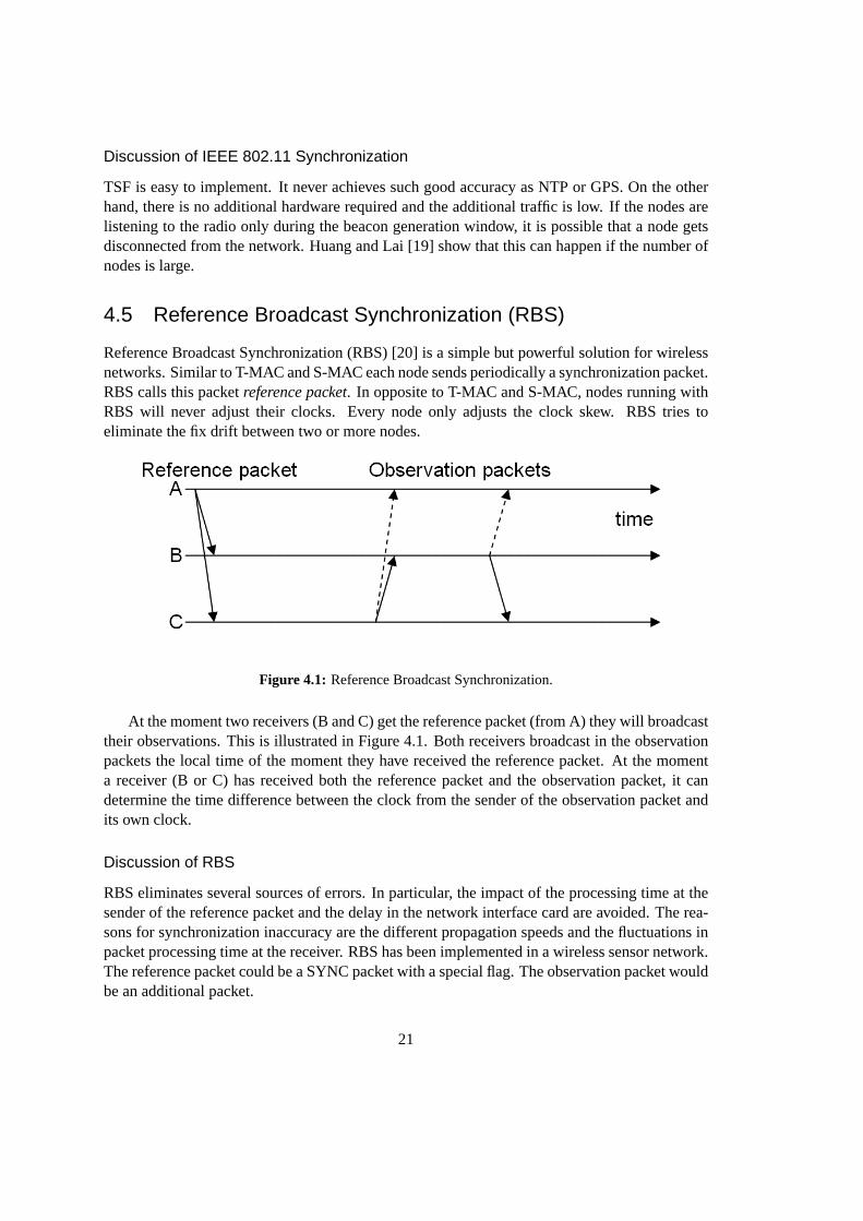
Reference Broadcast Synchronization (RBS) [20] is a simple but powerful solution for wirelessnetworks. Similar to T-MAC and S-MAC each node sends periodically a synchronization packet.RBS calls this packetreference packet. In opposite to T-MAC and S-MAC, nodes running withRBS will never adjust their clocks. Every node only adjusts the clock skew. RBS tries toeliminate the fix drift between two or more nodes.
Figure 4.1: Reference Broadcast Synchronization.
At the moment two receivers (B and C) get the reference packet (fromA) they will broadcasttheir observations. This is illustrated in Figure 4.1. Both receivers broadcast in the observationpackets the local time of the moment they have received the reference packet. At the momenta receiver (B or C) has received both the reference packet and theobservation packet, it candetermine the time difference between the clock from the sender of the observation packet andits own clock.
Discussion of RBS
RBS eliminates several sources of errors. In particular, the impact of theprocessing time at thesender of the reference packet and the delay in the network interface card are avoided. The rea-sons for synchronization inaccuracy are the different propagation speeds and the fluctuations inpacket processing time at the receiver. RBS has been implemented in a wireless sensor network.The reference packet could be a SYNC packet with a special flag. Theobservation packet wouldbe an additional packet.
21
4.6 Timing-sync Protocol for Sensor Networks (TPSN)
The Timing-sync Protocol for Sensor Networks (TPSN) [21] was designed for wireless sensornetworks. TPSN has two phases: The first is the level discovery phaseand the second is thesynchronization phase. The algorithm defines a root node before the first phase starts. A possibleelection algorithm is [22]. This root node is the top of a hierarchical structure and therefore getslevel 0 assigned. It broadcasts a leveldiscovery packet. The leveldiscovery packet contains theidentity and the level of the sender, i.e., 0 if the sender is the root node. All receivers of thesepackets become level i+1 and rebroadcast their leveldiscovery packet. If there are no packetslost due to collision, all nodes get a level assigned. The second phase isthen quite similar toNTP. The root node is stratum 0 and all nodes with level 1 synchronize their clock with the rootnode. In general all nodes from level i synchronize their clock with a node from level i-1.
In a wireless sensor network there might be many nodes in the 1-hop neighbourhood.Thus collisions might occur quite often. It is possible that a node will never receive alevel discovery packet. Therefore, TPSN introduces a local level discovery phase with anadditional levelrequest packet. All receivers have to answer this request by rebroadcast-ing their leveldiscovery packet. The requesting node collects all level information fromthelevel discovery packets and chooses the smallest level. Finally, it assigns itself ahierarchicallevel of this value plus one.
The lifetime of a sensor node is limited. Hence, a node will stop working at the momentit runs out of energy. TPSN does not need to care about that if this happens during the leveldiscovery phase, and before the node got a level assigned. However, the virtual tree could bebroken if this happens after that time. The disconnected nodes in the 1-hopneighbourhood stilltry to get synchronized, but their requests will never be answered if there is no other node in thevicinity with the same level as the dead one. In this case all disconnected nodes send again alevel request packet following the procedure of the local level discovery phase. After some timethe virtual tree will be repaired.
Discussion of TPSN
Simulation results show that TPSN achieves two times better results than RBS. Even over a5-hop distance the average error is only about 22.66 microseconds. [21] implements the RBSprotocol and TPSN in an IEEE 802.11 network. The hierarchical structure of TPSN can also beused for routing purpose if there is only node-to-sink communication required and the sink isthe top of the tree. A drawback of TPSN is that it requires a lot of control packets and that ittakes a rather long time until the nodes are synchronized.
22
Chapter 5
Simulation Environment
All protocols have been implemented in Omnet++ 3.1 [3]. The simulation model called mobilityframework version 1.0a5 has been used. All tests were executed on various PCs with WindowsXP or Windows 2003.
5.1 OMNeT++ 3.1 Overview
OMNeT++ is an open-source, component-based, modular and open-architecture simulation en-vironment. The short description of OMNeT++, according to the developer, is [3]: ”Its primaryapplication area is the simulation of communication networks and because of its generic andflexible architecture, it has been successfully used in other areas like thesimulation of IT sys-tems, queuing networks, hardware architectures and business processes as well. OMNeT++ israpidly becoming a popular simulation platform in the scientific community as well as inindus-trial settings. Several open source simulation models have been published,in the field of internetsimulations (IP, IPv6, MPLS, etc), mobility and ad-hoc simulations and other areas.” There isalso a commercial version of OMNeT++. It is called Omnest [23].
OMNeT++ is a discrete event simulator written in C++. An event can be everything. It canbe the start of a packet transmission, the detection of a movement of a sensor, a timeout and so on.All events are stored in a global event scheduler in strict time order. The simulation terminates assoon as there are no more events scheduled or the simulation reaches the user defined time limit.The component-based character of OMNeT++ provides the user with various features. Eachlayer of the network stack is a component. Therefore, it is simple to exchange individual layersto alter scenarios. In this work only the MAC layer was altered in the different experiments.Because it is an open-source application, it is possible to change the coreof the application, too.By changing a single value in the makefile, OMNeT++ creates, instead of an application with agraphical user interface (GUI), a simple program without any GUI.
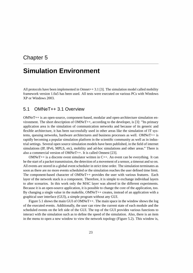
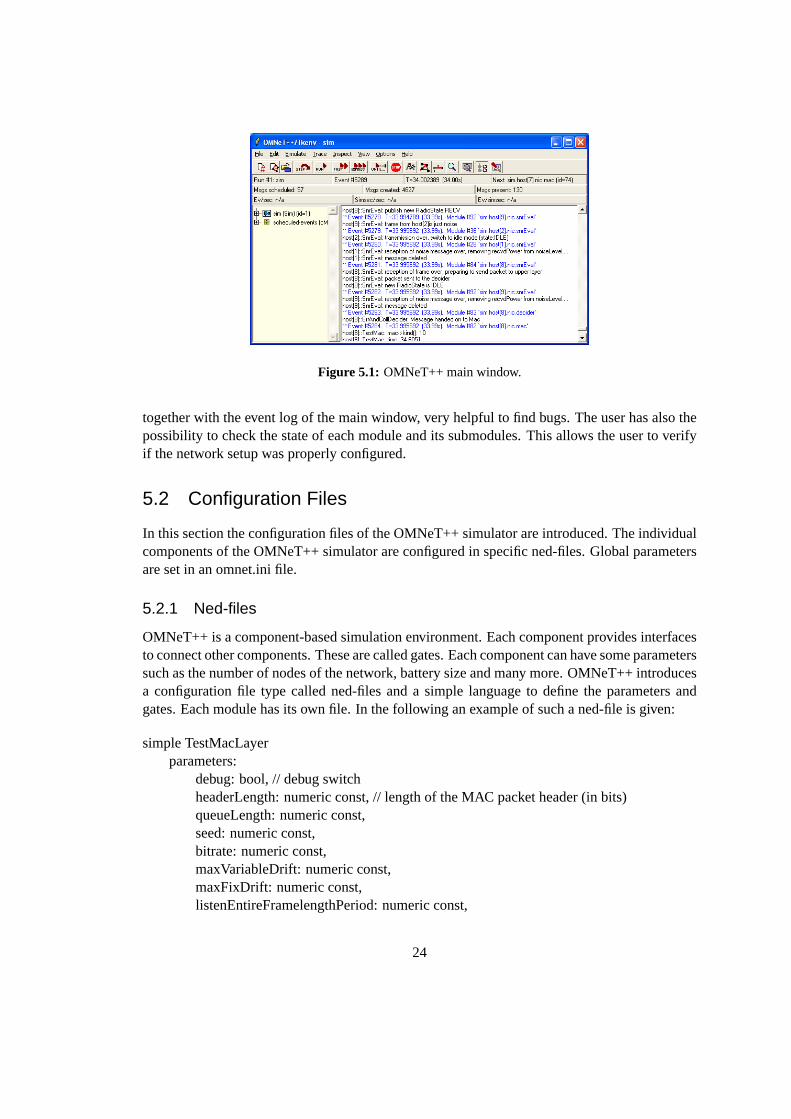
Figure 5.1 shows the main GUI of OMNeT++. The main space in the window showsthe logof the executed events. Additionally, the user can view the current state ofeach module and thescheduled events on the left side of the GUI. The top of the GUI provides various functions tointeract with the simulation such as to define the speed of the simulation. Also, there is an itemin the menu to open a new window to view the network topology (Figure 5.2). Thiswindow is,
23
Figure 5.1: OMNeT++ main window.
together with the event log of the main window, very helpful to find bugs. Theuser has also thepossibility to check the state of each module and its submodules. This allows the user to verifyif the network setup was properly configured.
5.2 Configuration Files
In this section the configuration files of the OMNeT++ simulator are introduced. The individualcomponents of the OMNeT++ simulator are configured in specific ned-files.Global parametersare set in an omnet.ini file.
5.2.1 Ned-files
OMNeT++ is a component-based simulation environment. Each component provides interfacesto connect other components. These are called gates. Each component can have some parameterssuch as the number of nodes of the network, battery size and many more. OMNeT++ introducesa configuration file type called ned-files and a simple language to define the parameters andgates. Each module has its own file. In the following an example of such a ned-file is given:
simple TestMacLayerparameters:
debug: bool, // debug switchheaderLength: numeric const, // length of the MAC packet header (in bits)queueLength: numeric const,seed: numeric const,bitrate: numeric const,maxVariableDrift: numeric const,maxFixDrift: numeric const,listenEntireFramelengthPeriod: numeric const,
The ned-file contains several sections. The first section describes theparameters of the mod-ule. In the example the simple module called ”TestMacLayer” has several parameters such asdebug, headerLength, queueLength. Each parameter needs a type declaration such as bool ornumeric const. The values for these parameters are defined in the omnetpp.ini file which ispresented in the next subsection. The second section contains the gates.Here, the possible con-nections to others modules are listed. The example provides four gates. A module can also havesome submodules. This helps to split up the code into multiple files. OMNeT++ furthermoresupports the exchange of submodules to achieve different scenarios.The submodules wouldalso be defined in the ned-file. OMNeT++ translates the ned-files into C++ code before it startscompiling the entire project. The syntax of the ned-files is much simpler than the syntax of thetranslated C++ code.
25
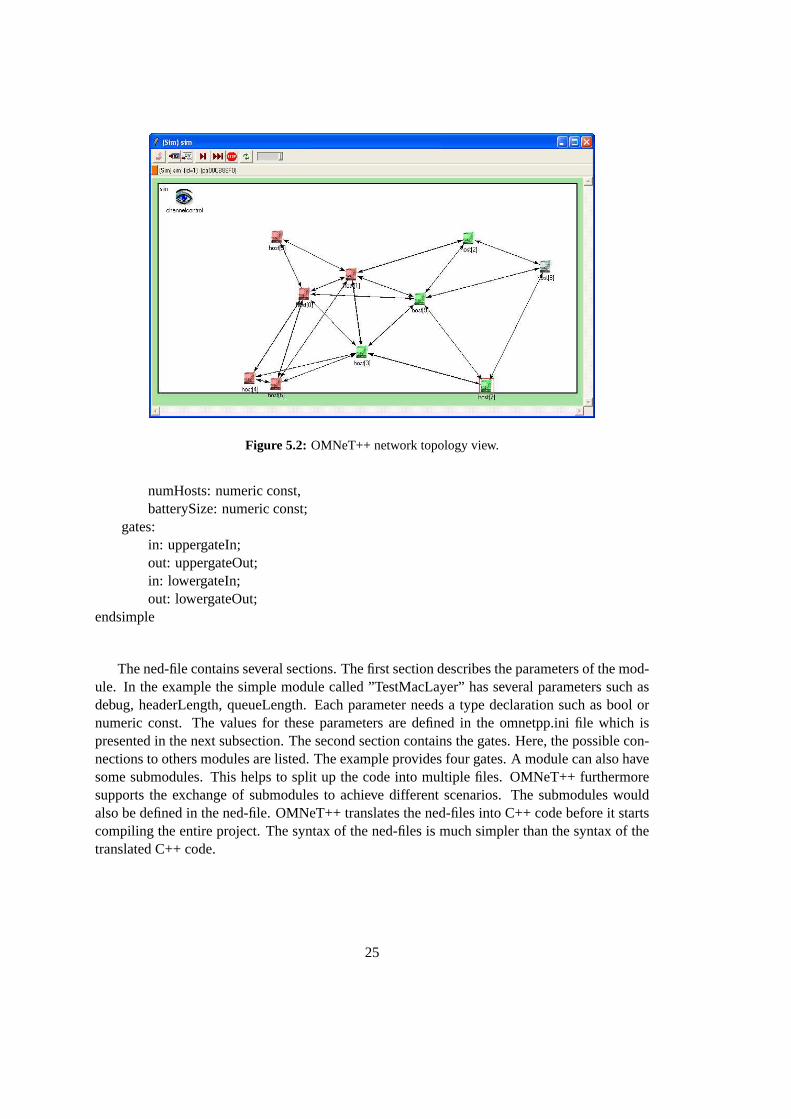
5.2.2 Omnetpp.ini
Instead of setting the parameters directly in the source code, OMNeT++ stores the parametersto configure the simulation in a file called omnetpp.ini. This file stores all parameterswhich arevalid for all modules. In the following a part of an example of such a file is shown:
The first parameter called ”debug” indicates whether debug statements areexecuted in theMAC layer or not. Debug information is provided if the value is 1. The debug parameter isdefined in the according ned-file (see Section 5.2.1). Another interesting value is ‘sim-time-limit‘. It defines the maximum duration of the simulation. The last three lines define the totalnumber of nodes and the dimension of the network. As there can be more thanone host it ispossible to define different parameters for each host. In this example sim.host[9].mobility.x andsim.host[9].mobility.y have different values than for all other hosts. This means that host 9 is seton position (100/100) in the simulation area, but all other nodes will be set randomly (indicatedby -1). All parameters defined in the ned-file must be set in omnet.ini. Otherwise the simulatorasks the user to provide these values during simulations start via a GUI.
26
5.3 Mobility Framework Overview
A cable connection between two devices is a one-to-one connection. There is always exactly onesender and one receiver of messages. OMNeT++ provides only suchone-to-one interfaces. Agate of a module can connect to only one gate of another module. There is nowireless networkconnection type with one sender and many receivers. This is however required in a wirelessmedium. Accordingly, such broadcast communications need to be developed. With the mobil-ity framework each host establishes connections to every other node inside its radio coverage.Moreover, the mobility framework provides functionality to model mutual interferences. Thisis required as in a shared wireless medium transmissions can disturb each other. Finally, theconnections are not fix. At the moment the nodes move around connectionschange accordingly.This is again handled by the mobility framework. The radio coverage of the nodes is modelledby two path-loss models called Free Space [24] and Two Ray [25]. In oursimulations we usethe Two Ray model. The calculation of the interference distanceDi and the maximum receivingdistanceDR of the Two Ray model is based on the transmission powerPT , the signal attenua-tion thresholdα, the minimal receiving powerPR to decode data and the antenna heightht. Theformulas for the interference and the maximum receiving distance look as follows:
Di =(
PT
10α10
· h4t
)1
4
(5.1)
DR =
(
PT
10
PR10
· h4t
)1
4
(5.2)
An important parameter in both equitations is the antenna height. A long antenna increasesthe interference distance and the receiving distance because of the power of 4.
5.4 Collecting Simulation Results in OMNeT++
OMNeT++ collects two kinds of simulation results. These are the ‘vectors‘, which contain allvalues of a specific parameter measured over time, and the ‘scalar‘ values, which are singleglobal values without a specific simulation time. A typical example of a ‘vector‘ isthe transportdelay of packets over time. An example of a ‘scalar‘ is the average transport delay of all datapackets. Both results are stored in according files called omnet.sca and omnet.vec respectively.Both are simple text files and contain the value descriptions and the values. For each of thesefiles there is an analysis tool provided by OMNeT++.
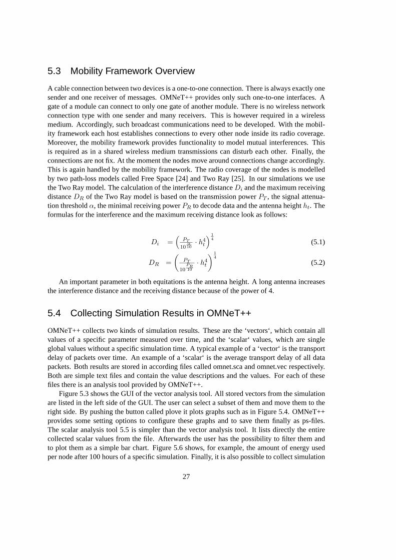
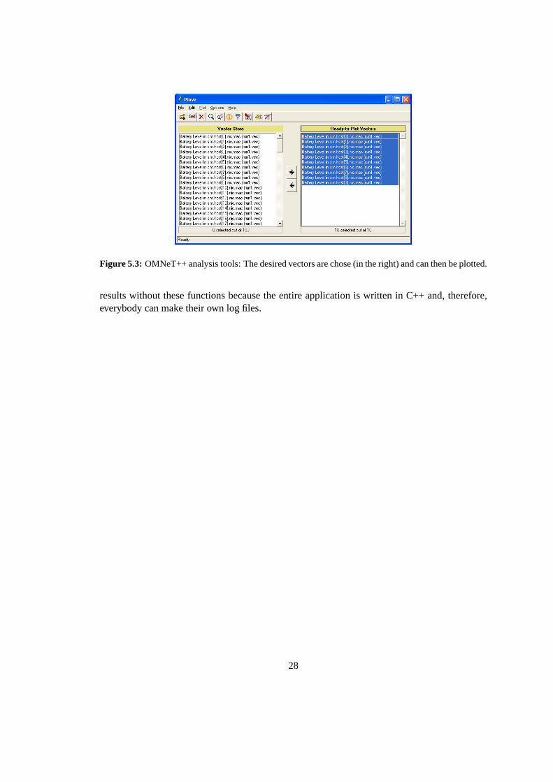
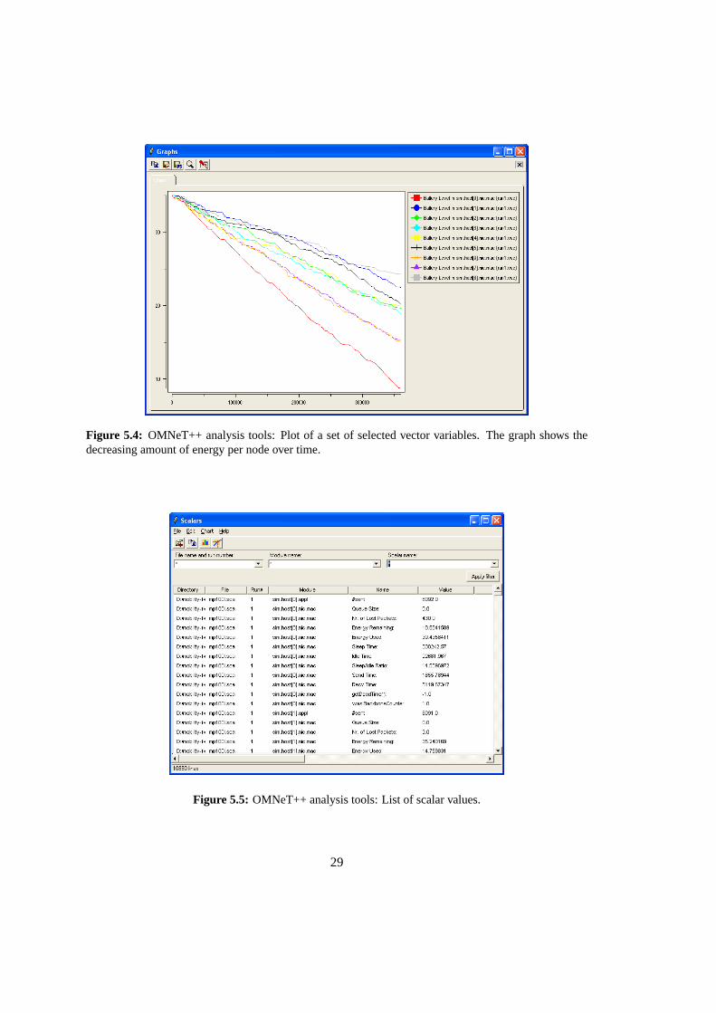
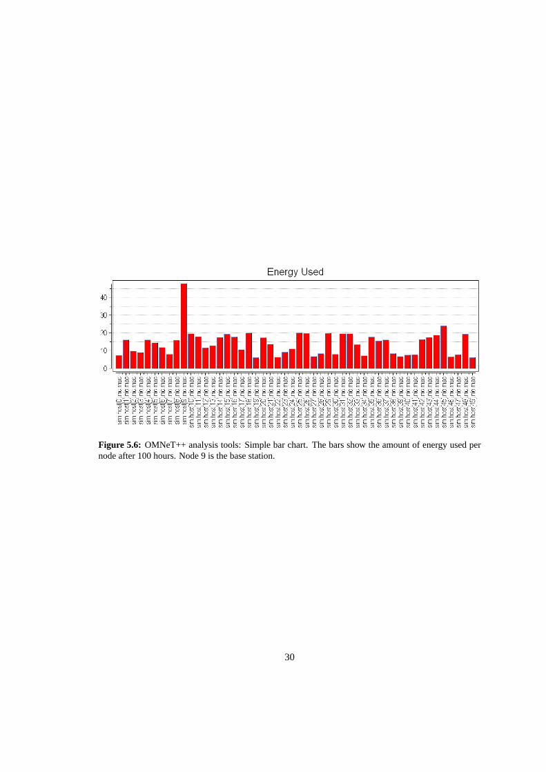
Figure 5.3 shows the GUI of the vector analysis tool. All stored vectors from the simulationare listed in the left side of the GUI. The user can select a subset of them and move them to theright side. By pushing the button called plove it plots graphs such as in Figure 5.4. OMNeT++provides some setting options to configure these graphs and to save them finally as ps-files.The scalar analysis tool 5.5 is simpler than the vector analysis tool. It lists directly the entirecollected scalar values from the file. Afterwards the user has the possibilityto filter them andto plot them as a simple bar chart. Figure 5.6 shows, for example, the amount of energy usedper node after 100 hours of a specific simulation. Finally, it is also possible tocollect simulation
27
Figure 5.3: OMNeT++ analysis tools: The desired vectors are chose (in the right) and can then be plotted.
results without these functions because the entire application is written in C++ and, therefore,everybody can make their own log files.
28
Figure 5.4: OMNeT++ analysis tools: Plot of a set of selected vector variables. The graph shows thedecreasing amount of energy per node over time.
Figure 5.5: OMNeT++ analysis tools: List of scalar values.
29
Figure 5.6: OMNeT++ analysis tools: Simple bar chart. The bars show the amount of energy used pernode after 100 hours. Node 9 is the base station.
30
Chapter 6
Synchronization-based CDS for WirelessSensor Networks
T-MAC and S-MAC allow communication between all nodes. Each node can create and sendpackets to all other nodes. Many possible applications for wireless sensor networks do not needto transmit data between sensor nodes, but rather have to report their data to a base station. Inother words: Many applications need only node-to-sink communication, whereby the sink isthe base station. In this work this property is used to extend the ideas of T-MAC and S-MACto achieve better results for such kind of applications. In detail an algorithmthat establishes arouting tree by using the SYNC messages of these contention-based protocols is provided.
6.1 Introduction
In T-MAC and S-MAC all nodes wake up periodically even if they have nothing to be sent. Thereare two reasons for that: First, they have to synchronise and second, they have to check whetherthere is another node waiting to send data to them. Under the assumption that there is mainlynode-to-sink communication required, there is no need that all nodes wakeup periodically aslong as routing is guaranteed. In this work we guarantee routing by establishing a connecteddominated set (CDS) which operates as backbone of the network. The entire traffic runs overthis backbone. A node outside the backbone sends its data directly to a backbone node. Forsuch non-backbone nodes there is no need to remain awake as long as there is no data from itssensors to be sent to the base station. Accordingly, these nodes can enter a long sleep period.Concerning the CDS setup, the following issues are considered:
• The base station is the sink of the CDS. The destination of all data is the base station.
• The number of nodes in the CDS should be as small as possible. Each node must have thepossibility to periodically disconnect from the backbone, as long as the algorithm is ableto maintain the connectivity of all nodes.
• Packets are routed over the backbone.
• The number of control traffic should be as small as possible.
31
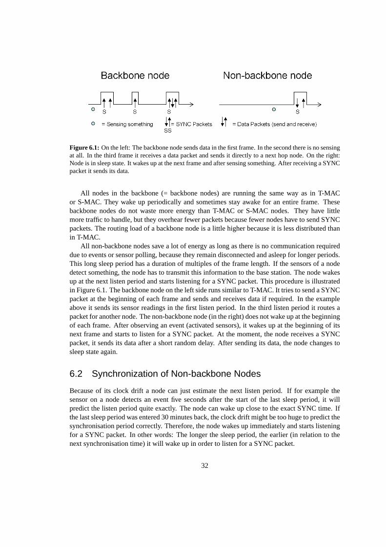
Figure 6.1: On the left: The backbone node sends data in the first frame. Inthe second there is no sensingat all. In the third frame it receives a data packet and sends it directly to a next hop node. On the right:Node is in sleep state. It wakes up at the next frame and after sensing something. After receiving a SYNCpacket it sends its data.
All nodes in the backbone (= backbone nodes) are running the same wayas in T-MACor S-MAC. They wake up periodically and sometimes stay awake for an entireframe. Thesebackbone nodes do not waste more energy than T-MAC or S-MAC nodes. They have littlemore traffic to handle, but they overhear fewer packets because fewer nodes have to send SYNCpackets. The routing load of a backbone node is a little higher because it is less distributed thanin T-MAC.
All non-backbone nodes save a lot of energy as long as there is no communication requireddue to events or sensor polling, because they remain disconnected and asleep for longer periods.This long sleep period has a duration of multiples of the frame length. If the sensors of a nodedetect something, the node has to transmit this information to the base station. Thenode wakesup at the next listen period and starts listening for a SYNC packet. This procedure is illustratedin Figure 6.1. The backbone node on the left side runs similar to T-MAC. It tries to send a SYNCpacket at the beginning of each frame and sends and receives data if required. In the exampleabove it sends its sensor readings in the first listen period. In the third listenperiod it routes apacket for another node. The non-backbone node (in the right) doesnot wake up at the beginningof each frame. After observing an event (activated sensors), it wakes up at the beginning of itsnext frame and starts to listen for a SYNC packet. At the moment, the node receives a SYNCpacket, it sends its data after a short random delay. After sending its data, the node changes tosleep state again.
6.2 Synchronization of Non-backbone Nodes
Because of its clock drift a node can just estimate the next listen period. If for example thesensor on a node detects an event five seconds after the start of the last sleep period, it willpredict the listen period quite exactly. The node can wake up close to the exact SYNC time. Ifthe last sleep period was entered 30 minutes back, the clock drift might be toohuge to predict thesynchronisation period correctly. Therefore, the node wakes up immediately and starts listeningfor a SYNC packet. In other words: The longer the sleep period, the earlier (in relation to thenext synchronisation time) it will wake up in order to listen for a SYNC packet.
32
If a non-backbone node, with some data pending for transmission, cannot send its data,because another node is sending its data, the node has to wait until this transmission is finished.Like in S-MAC and T-MAC the node tries to send its data with RTS/CTS after a random backoff.It is also possible that the first packet a node overhears is not a SYNC packet. In this case thenode treats the overheard data message as a SYNC packet. The sender of this data packet mightalso be a non-backbone node. Therefore, it is possible that a non-backbone node accepts requestsfrom another non-backbone node. This might occur if a non-backbone node looses connection tothe backbone, e.g, because the according backbone node fails or its SYNC packet was disturbedby another packet. In this scenario the non-backbone node remains awake and scans for othernodes. If a non-backbone node appears, it connects to that node, forwards its data to it and goesto sleep again. The neighbourhood node must have a connection to the backbone, otherwise itwould never send any packets. The benefit of this behaviour of the nodes in such a situation isobvious. Only one node needs to remain awake instead of both nodes and the risk of lost packetsare minimised. This behaviour produces more traffic but the sender of the data can go to sleepearlier and therefore it will save energy regarding both nodes.
6.3 Periodic Backbone Reconstruction
It would be possible, in a static network, to maintain a CDS unaltered once it hasbeen built.However, this would eliminate all the advantages over a system without CDS because a backbonenode needs more energy than a non-backbone node. As soon as one of the backbone nodes wouldrun out of energy, the entire branch of this network would be disconnected if there was no otherbackbone node which could overtake the work of the dead node. A partof the network would notbe able to send their data to the base station anymore. Moreover, there wouldbe no advantageof putting the non-backbone nodes into long sleep state if the CDS would never change, becausethis would not extend the lifetime of the entire network. Therefore, a solution that fuses theconcepts of CDS and T-MAC for wireless sensor networks needs to rebuild the CDS from timeto time. Furthermore, the solution should consider the current battery level of each node whileestablishing a new CDS to prevent that specific nodes are always selected into the backbone.
We propose two possible solutions to define a CDS in the next two sections. Both do notrequire additional packets. All data for building a CDS are attached to the standard SYNCpackets. Both solutions focus on static networks. There are additional mechanisms required tohandle mobility.
In contrast to pure T-MAC, it is important that all backbone nodes are able to send theirSYNC packets periodically. Otherwise, if there was no other traffic overheard, a non-backbonenode might have to wait too long until it detects a SYNC packet which enables itto connect tothe backbone.
6.4 Negotiation-based CDS (N-CDS)
In pure T-MAC and also in pure S-MAC all nodes are able to learn their 1-hop neighbourhoodfrom the SYNC packets. Every SYNC packet contains the ID of the sender and, therefore,
33
each node learns the IDs of its neighbourhood over time. This collection of node IDs and thetimestamp of the last receiving packet of specific node is the base informationrequired by theCDS building process of N-CDS. Adding this timestamp has the additional benefit that a nodeis able to detect nodes which are unavailable for a longer period (for example by running out ofenergy). If a node does not receive a SYNC packet from another node for a certain amount oftime, it assumes that the respective node is no longer available. A node has never a guaranteethat another node is no longer available because the SYNC packets are broadcast packets andthe transmission can always be disturbed, thus.
The base station is the root of a tree. The nodes of the tree are the backbone nodes. The basestation initialises the building of the tree. The establishment of the backbone occurs ringlikeaway from the base station. Therefore, each node in the backbone knows its parent node and allpackets for the base station are passed to these parent nodes.
6.4.1 CDS Building Process
In general the process consists of 4 steps. Each step is discussed in thefollowing:
1. The CDS nodes broadcast a packet called CDSSYNC containing its neighourhood infor-mation.
2. Each receiver becomes dominated and calculates its priority.
3. The dominated nodes locally exchange their calculated priorities.
4. The node with the highest priority is elected into the backbone.
Step 1
The CDSSYNC packet is an extension of a normal SYNC packet. In additionto the normalparameters for synchronization, it also contains the ID of each non-backbone node in the 1-hopneighbourhood of the sender.
Step 2
All receivers are called dominated if their ID is listed in the CDSSYNC packet. Adominatednode is a node that has a 1-hop connection to a backbone node and whichhas already receiveda CDSSYNC packet. The task of each dominated node is to figure out whether there is need tobecome a backbone node as well. There is only need if a node has not yetcovered nodes in itsneighbourhood. All receivers of a CDSSYNC packet will send all theirsubsequent data packetsto the sender of the first CDSSYNC they have received in the current CDS building process,i.e., of the first dominator they have learned. Each receiver marks its neighbours that are alsolisted in the CDSSYNC packet as dominated. Each dominated node calculates a priority afterthe reception of a CDSSYNC. This priority is the product of its own battery level and the numberof remaining nodes in its neighbourhood list that are not already backbone nodes or dominated.
34
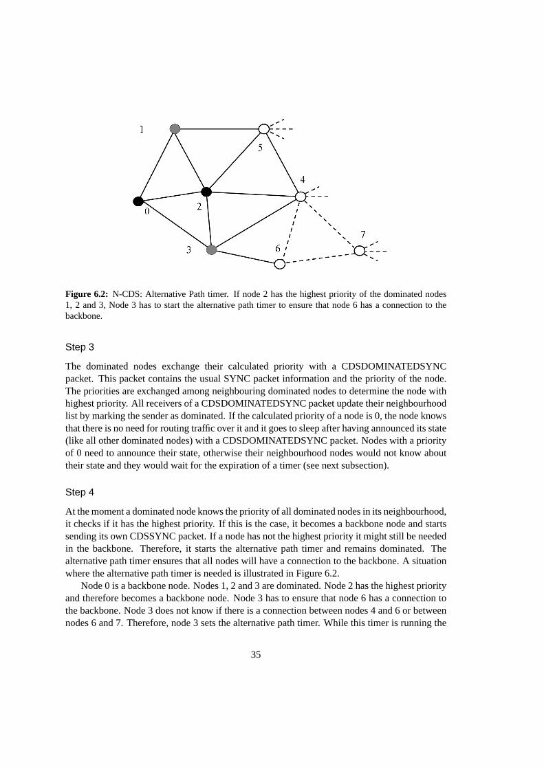
Figure 6.2: N-CDS: Alternative Path timer. If node 2 has the highest priority of the dominated nodes1, 2 and 3, Node 3 has to start the alternative path timer to ensure that node 6 has a connection to thebackbone.
Step 3
The dominated nodes exchange their calculated priority with a CDSDOMINATEDSYNCpacket. This packet contains the usual SYNC packet information and the priority of the node.The priorities are exchanged among neighbouring dominated nodes to determine the node withhighest priority. All receivers of a CDSDOMINATEDSYNC packet update their neighbourhoodlist by marking the sender as dominated. If the calculated priority of a node is 0, the node knowsthat there is no need for routing traffic over it and it goes to sleep after having announced its state(like all other dominated nodes) with a CDSDOMINATEDSYNC packet. Nodeswith a priorityof 0 need to announce their state, otherwise their neighbourhood nodes would not know abouttheir state and they would wait for the expiration of a timer (see next subsection).
Step 4
At the moment a dominated node knows the priority of all dominated nodes in its neighbourhood,it checks if it has the highest priority. If this is the case, it becomes a backbone node and startssending its own CDSSYNC packet. If a node has not the highest priority it might still be neededin the backbone. Therefore, it starts the alternative path timer and remains dominated. Thealternative path timer ensures that all nodes will have a connection to the backbone. A situationwhere the alternative path timer is needed is illustrated in Figure 6.2.
Node 0 is a backbone node. Nodes 1, 2 and 3 are dominated. Node 2 has the highest priorityand therefore becomes a backbone node. Node 3 has to ensure that node 6 has a connection tothe backbone. Node 3 does not know if there is a connection between nodes 4 and 6 or betweennodes 6 and 7. Therefore, node 3 sets the alternative path timer. While this timer is running the
35
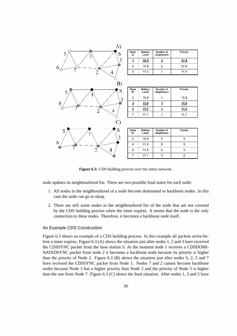
Figure 6.3: CDS building process over the entire network.
node updates its neighbourhood list. There are two possible final states for each node:
1. All nodes in the neighbourhood of a node become dominated or backbone nodes. In thiscase the node can go to sleep.
2. There are still some nodes in the neighbourhood list of the node that arenot coveredby the CDS building process when the timer expires. It seems that the node is the onlyconnection to these nodes. Therefore, it becomes a backbone node itself.
An Example CDS Construction
Figure 6.3 shows an example of a CDS building process. In this example all packets arrive be-fore a timer expires. Figure 6.3 (A) shows the situation just after nodes 1, 2and 3 have receivedthe CDSSYNC packet from the base station S. At the moment node 1 receives a CDSDOMI-NATEDSYNC packet from node 2 it becomes a backbone node becauseits priority is higherthan the priority of Node 2. Figure 6.3 (B) shows the situation just after nodes S, 2, 5 and 7have received the CDSSYNC packet from Node 1. Nodes 7 and 2 cannot become backbonenodes because Node 3 has a higher priority than Node 2 and the priority ofNode 5 is higherthan the one from Node 7. Figure 6.3 (C) shows the final situation. After nodes 1, 3 and 5 have
36
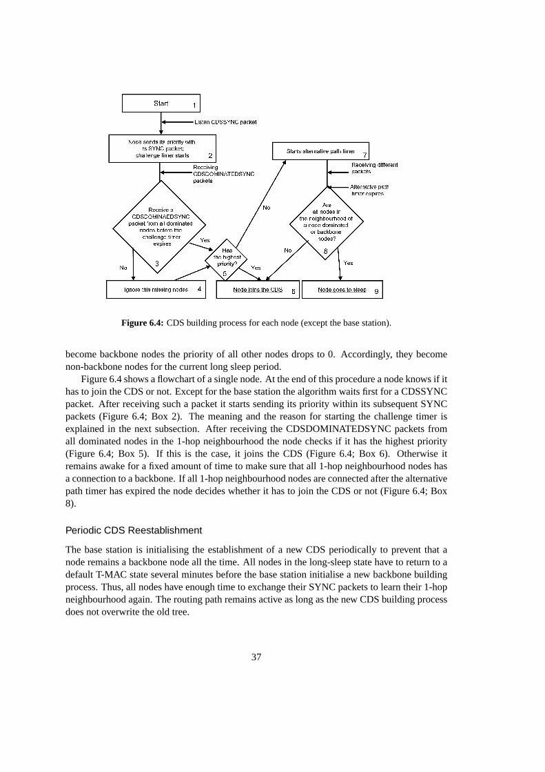
Figure 6.4: CDS building process for each node (except the base station).
become backbone nodes the priority of all other nodes drops to 0. Accordingly, they becomenon-backbone nodes for the current long sleep period.
Figure 6.4 shows a flowchart of a single node. At the end of this procedure a node knows if ithas to join the CDS or not. Except for the base station the algorithm waits first for a CDSSYNCpacket. After receiving such a packet it starts sending its priority within its subsequent SYNCpackets (Figure 6.4; Box 2). The meaning and the reason for starting the challenge timer isexplained in the next subsection. After receiving the CDSDOMINATEDSYNC packets fromall dominated nodes in the 1-hop neighbourhood the node checks if it has the highest priority(Figure 6.4; Box 5). If this is the case, it joins the CDS (Figure 6.4; Box 6).Otherwise itremains awake for a fixed amount of time to make sure that all 1-hop neighbourhood nodes hasa connection to a backbone. If all 1-hop neighbourhood nodes are connected after the alternativepath timer has expired the node decides whether it has to join the CDS or not (Figure 6.4; Box8).
Periodic CDS Reestablishment
The base station is initialising the establishment of a new CDS periodically to prevent that anode remains a backbone node all the time. All nodes in the long-sleep state have to return to adefault T-MAC state several minutes before the base station initialise a new backbone buildingprocess. Thus, all nodes have enough time to exchange their SYNC packets to learn their 1-hopneighbourhood again. The routing path remains active as long as the new CDS building processdoes not overwrite the old tree.
37
6.4.2 Packet Loss Problem
Broadcast packets can get lost. Therefore, each node has to retransmit packets which are in-volved in the CDS building process to guarantee a proper CDS setup. A fixed number of re-transmissions is not a good approach. In a network with low node density there is, in general, noneed to retransmit the packets as often as in a network with high density. Our first simulationshave shown that the sum of a small fixed value and the size of the neighbourhood list providesbetter results. If the number of retransmissions is too low, the CDS building process might bebroken. In such a case the CDSSYNC packets never arrive at the designated receivers. Of coursethis is not a disaster, if there was a complete CDS built once before. However, if a node has neverbeen affected by the building process, it will not know to which node it hasto send its packets.All downlink nodes of this node which are not connectable over alternative links will remainin the default sleep and listen states of T-MAC which is a waste of energy. Ifthe number ofretransmissions is too high, the time for establishing the tree becomes too long.
Another possible approach is to confirm a CDSSYNC packet with an ACK packet, but thiswould increase the amount of control messages. Each receiver of a CDSSYNC would have toreply the packet with an ACK packet. This would require in average at least 14 ACK packets toconfirm the CDSSYNC of a specific node in a network with an average node density of 15.
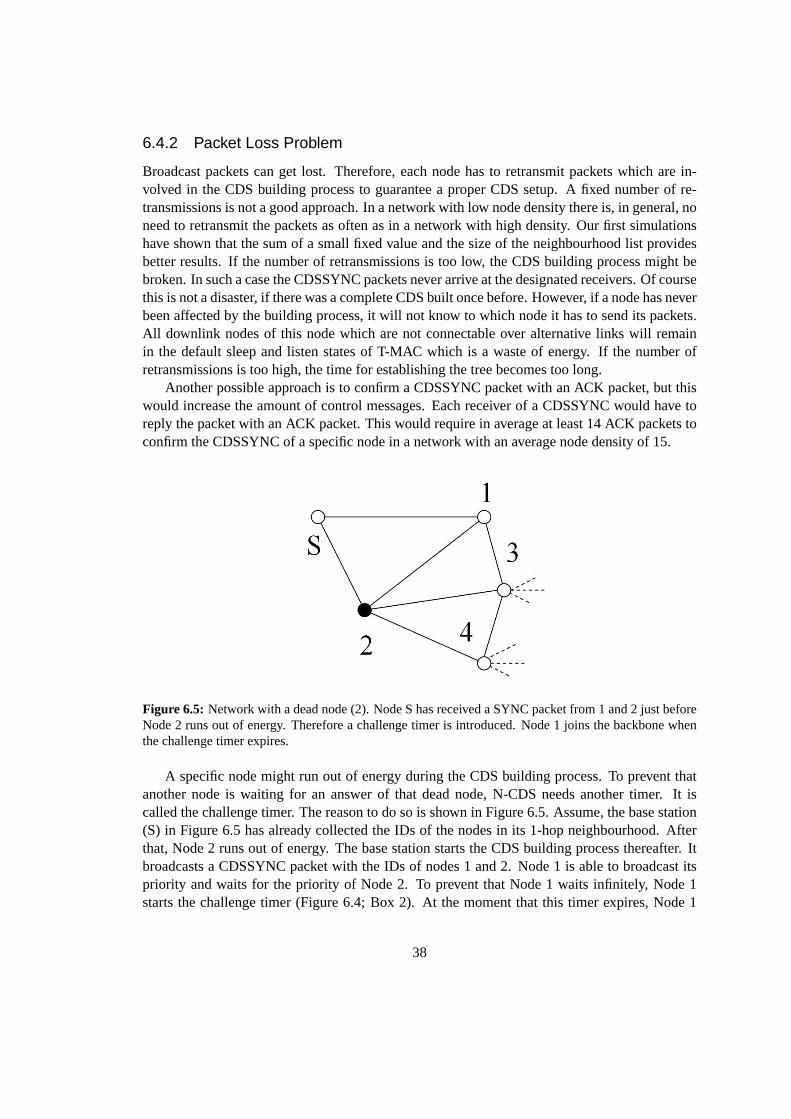
Figure 6.5: Network with a dead node (2). Node S has received a SYNC packetfrom 1 and 2 just beforeNode 2 runs out of energy. Therefore a challenge timer is introduced. Node 1 joins the backbone whenthe challenge timer expires.
A specific node might run out of energy during the CDS building process.To prevent thatanother node is waiting for an answer of that dead node, N-CDS needs another timer. It iscalled the challenge timer. The reason to do so is shown in Figure 6.5. Assume,the base station(S) in Figure 6.5 has already collected the IDs of the nodes in its 1-hop neighbourhood. Afterthat, Node 2 runs out of energy. The base station starts the CDS building process thereafter. Itbroadcasts a CDSSYNC packet with the IDs of nodes 1 and 2. Node 1 is able to broadcast itspriority and waits for the priority of Node 2. To prevent that Node 1 waits infinitely, Node 1starts the challenge timer (Figure 6.4; Box 2). At the moment that this timer expires, Node 1
38
deletes all dominated nodes from its neighbourhood from which it did not receive any priorityinformation (Figure 6.4; Box 4). In this example Node 1 becomes a backbonenode when thetimer expires (Figure 6.4; Box 6).
6.4.3 Discussion of N-CDS
The setup of the CDS is rather slow. Especially, if the network density is high,there are manynodes that are concurrently involved in the process. This causes problems because all nodes needthe priority of all nodes in their neighbourhood. The delay is affected by adjusting the numberof retransmissions of the CDSSYNC packets and by changing the duration of the timers. The N-CDS concept is a heuristic approach for establishing a CDS and, therefore, it rarely establishesa MCDS. However, the simulations have shown that N-CDS establish an adequate CDS whichis quite close to the MCDS.
6.5 Multi-Point Relay based CDS (MPR-based CDS)
A backbone node in N-CDS knows only its 1-hop neighbourhood. On the other hand, the moreinformation a backbone node has about its neighbourhood, the more advantage can be takenfrom the local connectivity. Accordingly, better results might be achieved, if a backbone nodeknows its 2-hop neighbourhood. Learning the 2-hop neighbourhood with all its connectionsimplies more costs than learning only the 1-hop neighbourhood, though. On the other hand, theCDS building process becomes simpler in particular the timer handling is noticeablesimpler.
6.5.1 Distribute Neighbourhood Information
At the moment a node becomes a backbone node, it should know its entire 2-hop neighbourhoodor at lest a good approximation of it. Additionally, the node should know the battery level ofall 1-hop neighbourhood nodes to avoid that a node would be selected asbackbone node all thetime. The simplest way to capture this information is to extend the SYNC packet with two fields.One contains the battery level of the sender and the other stores the ID of the sender of the lastSYNC packet. This implies, that each node must receive from each 1-hopneighbour at least asmany packets as there are nodes in the 1-hop neighbourhood of the neighbour. Thus, each nodelearns the 2-hop neighbourhood over time. As the focus of our work is onstatic networks, thelearning over time is acceptable.
6.5.2 CDS Building Process
In difference to N-CDS, the backbone node in the MPR-based algorithm defines the next nodeswhich join the backbone. That means that any backbone node defines in an internal routinethe further backbone nodes, at the beginning of its CDS building process. To implement thedecision process on a single node, rather than distribute it over neighbouring nodes as in N-CDS, is the reason why the building process of MPR-based CDS becomes simpler. The maintask of a dominator is to elect a subset of neighbour nodes as down-link dominators, so that theconnectivity to all 2-hop neighbours of the dominator is guaranteed. Therefore the backbone
39
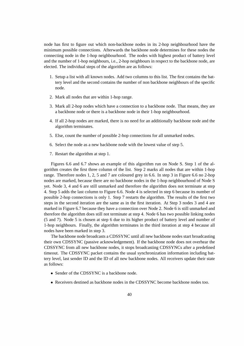
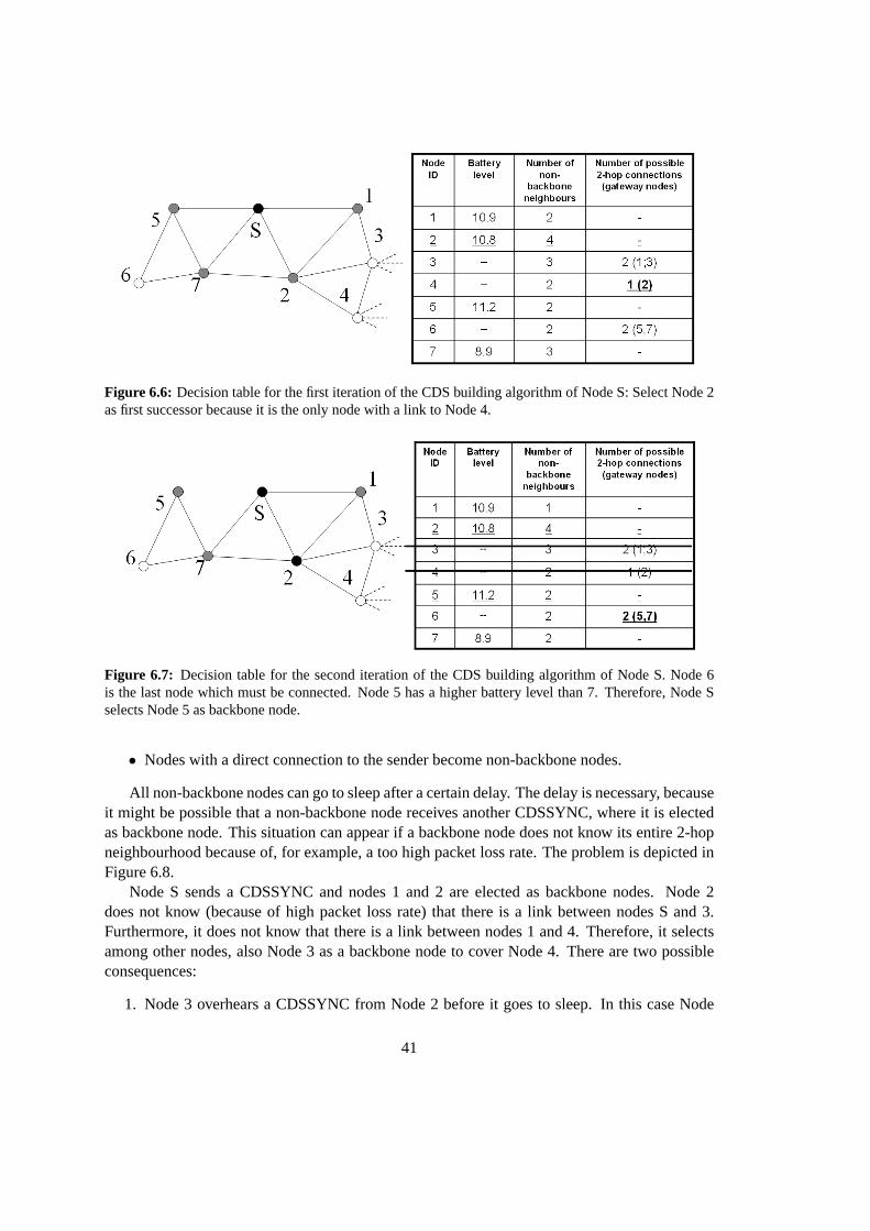
node has first to figure out which non-backbone nodes in its 2-hop neighbourhood have theminimum possible connections. Afterwards the backbone node determines for these nodes theconnecting node in the 1-hop neighbourhood. The nodes with highest product of battery leveland the number of 1-hop neighbours, i.e., 2-hop neighbours in respectto the backbone node, areelected. The individual steps of the algorithm are as follows:
1. Setup a list with all known nodes. Add two columns to this list. The first contains the bat-tery level and the second contains the number of non backbone neighbours of the specificnode.
2. Mark all nodes that are within 1-hop range.
3. Mark all 2-hop nodes which have a connection to a backbone node. That means, they area backbone node or there is a backbone node in their 1-hop neighbourhood.
4. If all 2-hop nodes are marked, there is no need for an additionally backbone node and thealgorithm terminates.
5. Else, count the number of possible 2-hop connections for all unmarked nodes.
6. Select the node as a new backbone node with the lowest value of step 5.
7. Restart the algorithm at step 1.
Figures 6.6 and 6.7 shows an example of this algorithm run on Node S. Step 1 of the al-gorithm creates the first three column of the list. Step 2 marks all nodes that are within 1-hoprange. Therefore nodes 1, 2, 5 and 7 are coloured grey in 6.6. In step 3 in Figure 6.6 no 2-hopnodes are marked, because there are no backbone nodes in the 1-hopneighbourhood of Node Syet. Node 3, 4 and 6 are still unmarked and therefore the algorithm does not terminate at step4. Step 5 adds the last column to Figure 6.6. Node 4 is selected in step 6 because its number ofpossible 2-hop connections is only 1. Step 7 restarts the algorithm. The results of the first twosteps in the second iteration are the same as in the first iteration. At Step 3 nodes 3 and 4 aremarked in Figure 6.7 because they have a connection over Node 2. Node 6is still unmarked andtherefore the algorithm does still not terminate at step 4. Node 6 has two possible linking nodes(5 and 7). Node 5 is chosen at step 6 due to its higher product of battery level and number of1-hop neighbours. Finally, the algorithm terminates in the third iteration at step 4because allnodes have been marked in step 3.
The backbone node broadcasts a CDSSYNC until all new backbone nodes start broadcastingtheir own CDSSYNC (passive acknowledgement). If the backbone nodedoes not overhear theCDSSYNC from all new backbone nodes, it stops broadcasting CDSSYNCs after a predefinedtimeout. The CDSSYNC packet contains the usual synchronization information including bat-tery level, last sender ID and the ID of all new backbone nodes. All receivers update their stateas follows:
• Sender of the CDSSYNC is a backbone node.
• Receivers destined as backbone nodes in the CDSSYNC become backbone nodes too.
40
Figure 6.6: Decision table for the first iteration of the CDS building algorithm of Node S: Select Node 2as first successor because it is the only node with a link to Node 4.
Figure 6.7: Decision table for the second iteration of the CDS building algorithm of Node S. Node 6is the last node which must be connected. Node 5 has a higher battery level than 7. Therefore, Node Sselects Node 5 as backbone node.
• Nodes with a direct connection to the sender become non-backbone nodes.
All non-backbone nodes can go to sleep after a certain delay. The delayis necessary, becauseit might be possible that a non-backbone node receives another CDSSYNC, where it is electedas backbone node. This situation can appear if a backbone node does not know its entire 2-hopneighbourhood because of, for example, a too high packet loss rate. The problem is depicted inFigure 6.8.
Node S sends a CDSSYNC and nodes 1 and 2 are elected as backbone nodes. Node 2does not know (because of high packet loss rate) that there is a link between nodes S and 3.Furthermore, it does not know that there is a link between nodes 1 and 4. Therefore, it selectsamong other nodes, also Node 3 as a backbone node to cover Node 4. There are two possibleconsequences:
1. Node 3 overhears a CDSSYNC from Node 2 before it goes to sleep. In this case Node
41
Figure 6.8: Node 2 does not know the link between nodes S and 3 due to packetloss. Node 3 eitherenters the backbone or not, depending on a timeout.
3 becomes a backbone node as well. This is a waste of energy, but else, there was analgorithm required which would allow a node to decline from becoming a backbone node.This would raise further complexity, though.
2. Node 3 does not overhear a CDSSYNC from Node 2 and enters the sleep state. In thiscase Node 2 continues to send CDSSYNC packets instead of switching backto shorterSYNC packets. This is some waste of energy at the backbone node, but not critical.
The duration of the long sleep period is the same as for N-CDS. Like in N-CDS, the MPR-based CDS has a period to learn the neighbourhood.
The MPR-based CDS has again been designed for static wireless sensornetworks. There-fore, deleting the entire neighbourhood nodes list after a long sleep period is a waste of infor-mation. It also takes some time to recollect the entire 2-hop neighbourhood information withthe SYNC packets. The MPR-based CDS mainly needs up-to-date informationabout the 1-hopneighbourhood. Therefore, MPR-based CDS deletes only the information of all 1-hop nodesand all 2-hop nodes where the last notification is older than a given threshold. The best choice ofthis threshold depends on the network structure. Even if the 2-hop neighbourhood is no longercorrect because of mobility or of the dead of one or more nodes, the algorithm still works well.The algorithm makes sure that all 2-hop neighbourhood nodes have a direct link to a backbonenode. If such a 2-hop neighbourhood node is no longer active the algorithm still works properly.If a 1-hop neighbourhood node x is no longer available, the CDS setup algorithm could raiseproblems. It would be possible that a backbone node selects exactly the dead node x as a newbackbone node to cover some 2-hop neighbourhood nodes.
42
6.5.3 Consequences of Packet Loss
As with N-CDS there are some packet loss impacts to be handled. A backbonenode broadcastsits CDSSYNC message without an automatic acknowledgement of the receivers. Therefore, thesender has to retransmit its CDSSYNC until it overhears a passive acknowledgement from itssubsequent backbone nodes. There are two ways to confirm the transmission. The first one is byoverhearing a CDSSYNC from a successor backbone node. If the initial dominator overhearssuch a packet, it is ensured that this successor has received the CDSSYNC packet. The other wayis to confirm the CDSSYNC packet by a CDSACKSYNC packet. If the receiver does not needto send a CDSSYNC packet, because all its 2-hop neighbourhood nodesare already covered, itconfirms the CDSSYNC with a CDSACKSYNC. This is a common SYNC packet with aspecialpacket type ID that signalises that this is a CDSACKSYNC packet.
At the moment a CDSSYNC sender overhears a reply from a new backbone node it willmark it in its neighbourhood node list. It removes this node from its subsequent backbone nodelist as well. Because the CDSSYNC packets contain the IDs of the remaining down-streambackbone nodes, the next CDSSYNC packets become shorter.
6.5.4 Advantage and Disadvantage of MPR-based CDS
The MPR-based CDS needs some memory on each node. The average number of items∆ in the2-hop neighbourhood list is related to the average number of 1-hop neighbourhood nodes d. Tocalculate these values following parameters must be given.
• n: Total number of sensor nodes in the entire network.
• r: Transmission range of the nodes.
• s: The side length of the network area.
The average node density d and the neighbour table size∆ are computed as follows:
d =n · r2
· π
s2
∆ = d + d2
Each node has to store the link informations about all 1-hop neighbourhoodnodes (d) andthe information about all 1-hop neighbourhood nodes of the 1-hop neighbourhood nodes (d·d).The equitation for d is taken from [26].
The memory allocation without hashing the data is 96 bits per item if the size of the nodeIDs is 32 bits. An item contains the ID of the node, the ID of the gateway node and a timestampof 32 bits in each case. So in total n·96 bits are required for the neighbour table without hashing.There is another table required for the CDS building process. This second table is quite small.It contains the ID and the CDS building status (backbone, non-backboneand not affected) ofa node. By hashing the data the size of each item becomes smaller. A hash code of 10 bitsis sufficient for most applications. 10 bits allow up to 1024 nodes in the 2-hopneighbourhood.
43
This provides enough IDs for a network with maximum network density of about 32 neighbours,which is a high density.
A real-world implementation should take care of the variable signal quality. If abackbonenode has to select a new backbone node, it normally prefers the ones closest to the border ofits maximum transmission range. Such nodes have normally a higher number of uncoveredneighbour nodes during the CDS building process. On the other hand, these connections haveoften poor link quality. Therefore, a real-world implementation should store the link-quality ofeach 1-hop node. During the CDS building process the backbone node should handle all 1-hopnodes with a poor link-quality as 2-hop nodes if there is a connection over another 1-hop nodeto these nodes.
MPR-based CDS is assumed to achieve better results than N-CDS because aMPR-basedCDS should create a smaller CDS, due to having more information. Therefore more nodescould go to sleep for a long period.
44
Chapter 7
Global Clock Synchronisation Gravitation
7.1 Problem of Virtual Clustering
T-MAC and S-MAC do not provide global time synchronisation. Only nodesinside the samevirtual cluster have their listen periods synchronised. All nodes regularly stay awake for anentire frame. Thus they have the possibility to detect other virtual clusters. If there are two ormore schedules from two or more nodes, the overhearing node adapts allschedules, but sends itsSYNC packet only in one listen period. With this mechanism the disjoint virtual clusters can beinterconnected. However, this means that the interconnecting nodes havea significantly higherpower usage. With our proposed algorithm we try to avoid interconnecting nodes with higherpower usage by maintaining a global schedule among all nodes.
Figure 7.1: Problem of Clustering.
Figure 7.1 shows an example of a network. In this simple case the node in the middle has
45
to take part in three virtual clusters and, accordingly, has to wake up 3 timesin a frame. Thepower usage for synchronization of this node will increase by a factor of 3 without data traffic.The authors of [27] have shown that even in a network with consisting of only 50 nodes, somenodes have to wake-up up to 4 times in a frame. If a node with more than one schedule runs outof energy, there might be no other node which can take over its job. If the nodes with two orthree slots in Figure 7.1 run out of energy, the network is divided into multiple parts. Therefore,it is desirable to avoid multiple schedules.
7.2 Local Adaptive Clock Assimilation Scheme (LACAS)
We try to achieve global synchronisation without a master node and without additional networktraffic. The proposed solution is called Local Adaptive Clock Assimilation Scheme (LACAS).LACAS avoids the drawback of virtual clusters. It is simple and it performswell in all simulatedscenarios. The basic principle bears resemblance to the physical gravitation of material. A hugebulk of material attracts a smaller one more than vice versa. Consequently, bothbulks of materialfuse after some time. In LACAS the cluster nodes represent the material andthe number of sentSYNC messages the gravitation force. Huge virtual clusters, which consist of more nodes, inaverage send SYNC packets more frequently and thus pull the small ones more than vice versa.Finally, both virtual clusters fuse to one.
Figure 7.2: Virtual Clustering in T-MAC: Node A belongs to an different cluster than nodes B and C.Node B, periodically stays awake for an entire frame in f2. It detects a SYNC packet from Node A, duringthis time. Afterwards, Node B wakes up two times per frame.
After deploying all nodes, each node runs initially a standard T-MAC protocol. Accordingly,a node starts to listen for already running nodes. If it hears another node, it adapts the schedulefrom the other node. Otherwise, it defines its own schedule and starts sending its SYNC packetat the beginning of its listen period. This implies the creation of a new virtual cluster. Sooneror later a node of a specific virtual cluster overhears a SYNC packet from a node of a differentvirtual cluster if the node shares the space of both clusters. Normally, this occurs during theperiod when a node is awake for an entire frame. T-MAC and LACAS react in a different way atthe moment a node detects a SYNC packet from a different cluster. This is illustrated in Figure
46
7.2. In T-MAC, Node B listens to both schedules until death by awaking twice ineach frame assoon a s both schedules are known, i.e., after frame f3 in Figure 7.2.
A node with LACAS never has two schedules. It shifts its own schedule to a given gravitationadaptation percentageα (e.g.α = 5%) towards the schedule of the node it has received a SYNCmessage from. Additionally, it extends its listen period over both schedules. The length of thislisten period is the time span over the own schedule and the schedule learned from the overheardSYNC from the other virtual cluster. Having spanned both clusters, the according node starts tocontract its schedule again. Due to the schedule expansion, the power consumption temporarilygoes up, but this effort is insignificant compared to the fact that the clusters can be eliminated inthis way.
Figure 7.3: Operation of LACAS: Node B stays awake for an entire frame in f2. During this time itdetects a SYNC packet from Node A. It adapts this schedule byα. The next awake period of Node B isextended such that it spans the schedule of nodes A and C.
Figure 7.3 is an example of such a cluster fuse. Node A belongs to a different cluster thannodes B and C in f1. In f2 Node B stays awake for an entire frame and detects a SYNC packetfrom Node A. Therefore it extends its regular listen period over both schedules inf3. Addition-ally, its own schedule shiftsα towards Node A. Node A stays awake for an entire frame in thesecond half of f4 and for the first half of f5 and detects the SYNC packet from Node B. LikeNode B, Node A extends its listen period over both schedules and shifts its schedule towardsNode B in f6. This means, that this small network is connected from now. Betweenf6 andfn
both clusters mutually exchange SYNC packets and thus attract each other.Additionally thenodes contract their schedule again. The fusion process finishes infn, because all three nodeshave the same schedule. Simulations have shown that in general it takes lessthan 3 minutes toachieve a common schedule in a network consisting of 200 nodes. On the other hand, a sensornetwork is in general designed for a long network lifetime, e.g., to work for ayear or more.Moreover, the physical deployment of the nodes takes some time. Therefore, it is acceptablethat it takes some minutes until the clocks are synchronized.
47
Figure 7.4: Operation of LACAS: The value forα is in this example too high and therefore the networksbreaks in two parts.
The value forα has a huge influence considering performance. Ifα is too low it will takea long period until the schedules fuse to one global schedule. On the otherhand, ifα is toohigh, the connection between the nodes might be broken all the time. This problem is illustratedin Figure 7.4. In this example the value forα is too high. All nodes reach their neighbourswith a SYNC packet in f1. Therefore, the network is connected. Afterwards there are too manybackground noises between nodes B and C and the SYNC packets are lost in f2. However nodesA and D are able to send their SYNC packets and therefore nodes B and C drift away from eachother. This drift is too high and the SYNC packet of node B misses the listen period of the nodeC in f3 and vice versa.
This disconnection is not a basic problem. The clusters will be reconnectedagain when theylisten for an entire frame. However, the disconnection increases the period until the schedulesfuse. At the moment there is only one global schedule a highα is better than a small one.LACAS has only to compensate the clock drift of each node at this point of time, as it hasalready eliminated the virtual clusters. Therefore, the value forα switches in our simulationsto 50% at the moment the CDS building process is finished. At this time all nodes should besynchronized. Furthermore, all backbone nodes at the leaves of the CDS adapt the schedulelearned from the SYNC packet to 100%. Such nodes need to be synchronized only with onenode because all other nodes neighbours are sleeping. Therefore,these neighbours will neversend a SYNC packet. This feature of LACAS applies only if the network provides a CDS asbackbone.
7.3 Discussion of LACAS
LACAS prevents the virtual clustering and saves a lot of energy. The networks of T-MAC andS-MAC are broken at latest at the moment when all nodes at the borders of the virtual clustersdie. In general, they die earlier than the other nodes because they have tolisten to more thanonly one schedule. LACAS eliminates virtual clusters. It eliminates also the borders between
48
the clusters. This increases the lifetime of a wireless sensor network.
49
Chapter 8
Implementation and Evaluation
To evaluate our approach we implemented the algorithms in the Omnet++ network simulatorwith the Mobility Framework version 1.0a5 (see Chapter 5).
8.1 Simulation Setup and Parameters
We implemented three different MAC protocols.
• T-MAC according to its authors [8]
• N-CDS with LACAS
• MPR-based CDS with LACAS
Nodes in sensor networks are unsynchronised in the beginning. To synchronize the nodes, N-CDS and MPR-based CDS implement LACAS. In all simulations LACAS added nosignificantoverhead to the CDS-based protocols. Therefore, we decided to compare the protocols to theoriginal T-MAC implementation, which provided fully synchronised nodes atsimulation start. IfT-MAC would be run with LACAS too, it might slightly loose performance, though this wouldhardly be measurable.
The payload generator and the network structure is the same for all three protocols. Thepayload generator creates approximately 1 packet per node per minute. There is no data trafficduring the first 400 seconds. LACAS and the CDS-based approachesare designed for staticnetworks. Therefore, there is no mobility in the network. The network consists of 50, 100or 200 nodes. The average number of 1-hop neighbourhood nodes per node ,i.e., the networkdensity, is 10 or 15. The network structure is random. We have chosen for each network sizeand network density 10 random networks, in which all nodes have a connection (some overseveral hops) to the base station. Totally, 60 different networks are simulated for the 3 differentMAC protocols. Each simulation stops after 100 simulated hours. So, in total 18’000 hours aresimulated. Each node has an individual clock drift. The maximum clock drift between any 2nodes is 2µs per second. This is still more than the maximum clock drift of the ESB sensorplatform from [1]. The total drift is a sum of two parameters. One is the fixed drift of the node.Each node defines its fixed drift at the beginning of each simulation. This fixed drift simulates
51
the incorrectness of each oscillator compared to the correct time. The othervalue is the variabledrift that changes all the time. This is the jittering of the oscillator.
There is no check on the network layer, whether a specific packet has already been sent tothe next node or not. This means the generation of duplicates is not prevented. For example,assume node A sends a packet to node B. B receives the data and starts sending its ACK packet.This ACK packet does not arrive at node A because of too much noise.Thus, A has to resend thepacket. However B already received the packet and sends the message to the next node. Afterthe retransmission of this packet from A to B, B does not realise that it has already received thisdata packet. Therefore it will send it twice. This happens rarely. Moreover, all three protocolshave the same network layer and are therefore faced with the same problem.
The specification of the simulated hardware is according to experienced values from the ESBsensor platform developed at FU Berlin [1]. All important parameters arelisted in Table 8.1.
SPECIFICATION VALUE
Frame length 610 msPower consumption in sleep mode 0.005 mAPower consumption in idle mode 4.7 mAPower consumption in send mode 5.2 mAPower consumption in receive mode 4.7 mABuffer size 25 packetsBattery level at start 45 mAhPath loss model TwoRayAntenna height 0.17mBit rate 115.2E+3 bits/secondSNR threshold 5 dBTransmitter power 0.75 mWCarrier frequency 8.68E+8 HzThermal noise -98 dBSensitivity -95 dBListen entire frame length all 21.35 secondsMaximum contention window 2.56msTA 6.444ms
Table 8.1: Sensor platform dependent parameters.
The radio consumes most power on a wireless sensor node. A node in sleep state (the radiois off), only uses 5µA. A node in idle state (the radio is on) consumes 940 times more power(4.7 mA) than in the sleep state. The transmitter power is 0.75 mW. The two-ray model is chosenas path-loss model in our simulations.
With an antenna height of 17cm and a carrier frequency of 8.68E+8 Hz anode has an ex-pected transmission range of about 37m. The interference range is about 52m. The ESB of [1]use, per default, a bitrate of 19200 kbits per second, but the hardwareis ready for higher band-widths of up to 115200 bits. The bandwidth in our simulations is, accordingly, set to 115200
52
bits per second. The base station is placed always in the centre of the playground.
8.1.1 Packet Definitions
The following tables define the specific packets for all 3 MAC protocols.
NAME LENGTH IN BIT
Preamble 16Packet Type 8Source ID 32Timestamp 32CRC 16
Table 8.2: SYNC packet for T-MAC and N-CDS.
Table 8.2 describes the structure of a SYNC packet used in T-MAC and N-CDS. Like allother packets it contains a preamble, a packet type and a CRC part. The preamble makes surethat the receiver interprets the start of the data of this packet correctly.The CRC part checkswhether the data of this packet has been transmitted correctly. The packettype informs thereceiver that this packet is a SYNC packet. The source ID is the system-wide unique ID of thesender node. The timestamp contains the relative time to send the next SYNC packet. This is afloat value between 0 and the maximum length of the frame.
NAME LENGTH IN BIT
Preamble 16Packet Type 8Source ID 32Timestamp 32Last Node ID 32Battery Level 32CRC 16
Table 8.3: SYNC packet for MPR based CDS.
To setup the MPR-based CDS two additional values are required to learn the2-hop neigh-bourhood as well as the battery level of all 1-hop neighbourhood nodes. The according SYNCmessage to setup the MPR-based CDS is shown in Table 8.3. The two additionalparametersare the ID of the last node and the battery level. The ID of the last node has, like the ID of thesource, a size of 32 bits. The battery level is a float value and describesthe battery level of thesender. This could alternatively be an integer value if the hardware of thenodes provides thebattery level as an integer value.
The RTS packet (Table 8.4) has the same structure for all three MAC protocols. RTS isa broadcast packet similar to a SYNC packet. Additionally, it has a field for the ID of the
53
NAME LENGTH IN BIT
Preamble 16Packet Type 8SourceID 32DestinationID 32NAV 8CRC 16
Table 8.4: RTS and CTS packets.
destination of the packet, though. It furthermore provides the network allocation vector (NAV)to define the length of the subsequent data packet. This value is useful for all the other nodeswhich overhear the transmission. Using the NAV each receiver can calculate how long the entiretransmission of the data packet will take. They have to be quiet during this time (except for theFRTS just after the CTS packet). A CTS packet has exactly the same structure as the RTS andis again the same for all three protocols.
NAME LENGTH IN BIT
Preamble 16Packet Type 8SourceID 32DestinationID 32CRC 16
Table 8.5: DS, FRTS and ACK packets.
All DS, FRTS and ACK packets (Table 8.5) have a similar structure as a RTS packet. Thedifference between these packet types and a RTS packet is only then missing NAV. There is noneed for this field for this packet type and, therefore, it is not used.
NAME LENGTH IN BIT
Preamble 16Packet Type 8SourceID 32DestinationID 32Length of payload 8Payload variableCRC 16
Table 8.6: Data packets.
54
Each data packet (Table 8.6) has a payload of variable length. Each fieldwith a variablelength needs another field, in which the length of the variable field is indicated.Therefore, adata packet has also a field (length of the payload) in which the size of the payload is defined. Inthe simulations all data packets have a fixed payload of 164 bits.
NAME LENGTH IN BIT
Preamble 16Packet Type 8SourceID 32Timestamp 32Priority 32CRC 16
Table 8.7: DOMINATEDCDSSYNC packet of N-CDS.
Only N-CDS needs a packet called DOMINATEDCDSSYNC (Table 8.7). Itis similar to adefault SYNC packet with an extended field called ”Priority”. It is an integer value as long asthe battery level of a node is stored as an integer value. Otherwise, it might be mapped to a floatvalue. The priority of a node is the product of the number of free nodes inthe neighbourhoodand the battery level of the node. It is used for the dominator election. This packet is sent bydominated nodes to exchange their priorities.
NAME LENGTH IN BIT
Preamble 16Packet Type 8SourceID 32Timestamp 32length/number of dominated nodes 8Destination IDs n · 32CRC 16
Table 8.8: CDSSYNC packet for N-CDS.
The CDSSYNC packet for N-CDS (Table 8.8) is also used in the dominator election process.A backbone node sends a CDSSYNC packet to announce its state and to define the node whichwill be marked as dominated. The packet has a variable length due to the varying number ofdestination IDs (n).
The two remaining packet types are the CDSSYNC packet and the CDSACKSYNC packetfor the MPR-based CDS. The CDSSYNC packet contains the lists of all subsequent backbonenodes. CDSACKSYNC is the confirmation packet of a CDSSYNC packet receiver which hasno further backbone nodes. It has exactly the same structure as the default SYNC packet ofthe MPR-based CDS. The CDSSYNC packet for the MPR-based CDS is shown in Table 8.9.It has the following characteristics: All fields except the two added field called ‘length/number
55
NAME LENGTH IN BIT
Preamble 16Packet Type 8SourceID 32Timestamp 32LastNodeID 32BatteryLevel 32length/number of dominated nodes 8Destination IDs n · 32CRC 16
Table 8.9: CDSSYNC packet for MPR based CDS.
of dominated nodes‘ and ‘Destination IDs‘ have the same structure as the SYNC packet of theMPR-based CDS (see Table 8.3). These two new fields have the same structure as the addedfields from the SYNC packet to the CDSSYNC in N-CDS (see Table 8.8).
8.1.2 Simulation Details for T-MAC
A real-world T-MAC implementation would have to include virtual clustering. Each virtualcluster decreases the lifetime of the entire network. But, we want to compare our protocols withthe standard T-MAC protocol as implemented in the original work, so that we can rely on thoseresults. Due to deployment and radio transmission impacts, virtual clustering isdifficult to besimulated. Therefore, virtual clustering would have to be evaluated in realworld implementa-tions. In our simulations we do not consider virtual clustering. In the evaluation of LACAS theimpact of virtual clustering is considered, though. The T-MAC implementation does not providerouting support. Therefore, at the beginning of each simulation the routingtables for each nodeare precalculated. To achieve this, each node figures out which node inits neighbourhood isone hop closer to the base station than itself and defines this node as the backbone node, whereall packets are routed to. This eliminates all routing issues and additional routing communica-tion on the routing layer. This simple shortest-path algorithm is the same approach as used inthe original paper of T-MAC [8]. Any implementation of a routing algorithm would imply im-pacts that would be difficult to be assessed. Accordingly, our approach is compared to a optimalT-MAC implementation with optimal routing support.
Finally, all nodes in the original paper are arranged in a fixed grid. There is no routingover links with poor link-quality. Because in our simulation all nodes are placed randomly, ourshortest-path algorithm only considers links with good link quality to achieve a similar situationas in the original paper. Therefore, all nodes that are farther away than 95% of the maximumtransmission range are not considered. If we would consider all possible links in the shortestpath algorithm, the benchmark of the T-MAC simulations would be less meaningfulbecause theinfluence of the poor links is difficult to sort out. As a consequence we compare our protocolto a T-MAC implementation with artificial and optimal solutions for the problems of virtual
56
clustering and routing.
8.1.3 Simulation Details for N-CDS and the MPR-based CDS
SPECIFICATION VALUE
Rebuild dominator set each hourLong sleep duration per hour 50 minutesSYNC schedule adaptation 5% in starting periodSYNC schedule adaptation 50% if CDS existsNeighbourhood table size unlimited
Table 8.10: Technical specifications for N-CDS and MPR-based CDS.
Table 8.10 shows some configurable settings which are valid for the N-CDS and for theMPR-based CDS. For both protocols all nodes have 10 minutes for updating their neighbour-hood tables. We assume that the memory of each node is large enough to storethe entire neigh-bourhood table. All nodes have a random initial wake up time between 0.1 seconds and 30.1seconds after the start of the simulation. This means that a node starts working within this time.
Specific Details for N-CDS
In N-CDS the challenge timer is set to 30 seconds. After a node becomes dominator it sendsits relevant information 12 times plus once more for each node in the 1-hop neighbourhood.This is a rather high value, but the additional cost is low and it reduces the risk of breakingthe CDS setup process. Before a node, which does not become a backbone node, goes to sleepit sends a CDSDOMINATEDSYNC packet only 5 times plus once more for each node in the1-hop neighbourhood. The simulations wait 200 to 230 seconds until the CDS building processis started for the first time. N-CDS needs this time to let the nodes synchronise and to learn the1-hop neighbourhood.
Specific Details for MPR-based CDS
In the MPR-based CDS the simulations wait 300 to 330 seconds until the CDS building processis started for the first time. MPR-based CDS needs this time to let the nodes synchronise and tolearn their 2-hop neighbourhood.
8.2 Simulation Results
The most important evaluation parameter we investigate is the power usage of the nodes. Thisvalue is analysed concerning two different aspects. First, there is the overall battery usage whichdescribes how much power the entire network requires to fulfil all requested operations. Thesecond value is the battery usage of each node.
57
8.2.1 Convergence of SYNC Period with LACAS
Before showing the results of the coordinated sleeping, we show the analysis of LACAS. Figure8.1 shows the average duration of the listen period, i.e., of the schedule length. This is the timedifference between the earliest detected schedule and the last scheduleplus an additional backoffof 7ms. This backoff ensures that the nodes are able to detect the SYNC packets even after someshifts of the schedules. Three different network sizes, consisting of 50, 100 and 200 nodes, havebeen evaluated. We calculate the error bars each 5 second except forthe simulation with 200nodes. For readability reasons not all standard deviations are shown inFigure 8.1 (c).
0
100
200
300
10 100 1000
Sch
edul
e Le
ngth
[ms]
Time [s]
50 Nodes
(a) Network, consisting of 50 nodes.
0
100
200
300
10 100 1000
Sch
edul
e Le
ngth
[ms]
Time [s]
100 Nodes
(b) Network, consisting of 100 nodes.
0
100
200
300
10 100 1000
Sch
edul
e Le
ngth
[ms]
Time [s]
200 Nodes
(c) Network, consisting of 200 nodes.
Figure 8.1: Length of the SYNC packet exchange period in a MPR-based CDS network.
The graphs rise first to the maxima schedule lengths which are between 177msand 189ms.The nodes wake up for the first time between 0 and 30s. Afterwards they choose their ownschedule or adapt an already existing one. Accordingly, initially they haveonly one schedule.Therefore, the values are quite low in the beginning. Quickly the nodes detect other schedulesand listen to all of them. At this point the graphs begin to raise to the maxima values.Afterwardsthe different schedules fuse to one and the graphs drop down again. The CDS establishingprocess starts at 320s. This decreases the number of SYNC packets and therefore the graphs
58
rise to a local maximum. Without optimization, the gravitation adaptation percentageα wouldremain 5% (see Chapter 7) and the graphs would converge to 13ms. Due to the CDS algorithm itis possible to change the factor to 50%, though. Thus, LACAS finally converges to 10 ms. Theduration of the SYNC packet exchange period in T-MAC is 7ms. Accordingto the real worldimplementation of S-MAC with 50 nodes done in [27] some nodes have to wake-up up to 4times in a frame. In a rather poorly performing network the authors have shown that 66% of allnodes follow 2 schedules and 34% follow even 3 schedules. We assume that these schedules aredisjoint. T-MAC und S-MAC do not differ concerning virtual clustering. To give an idea of thepower savings that could be achieved with LACAS, we estimate the performance of MPR-basedCDS enhanced with LACAS and T-MAC with virtual clustering for the given network. T-MACwith virtual clustering requires a power supply of 3.85 mAs per frame over all network nodesand without data traffic. The equitation to calculate the average schedule costs∆ in T-MAClooks as follows:
The entire network consisting of 50 nodes needs 235mA in idle mode. This value must bemultiplied with the mean schedule length (listen period length) in a frame. The schedule lengthof T-MAC consists of the time spent to follow all known schedules. On the other hand, MPR-based CDS with LACAS only requires 2.35 mAs (235mA· 10ms) in a frame if all nodes areawake. With LACAS the schedule length is fixed to 10ms for every network node. In 100 hoursor more this would make a difference. However, also compared to the other experiments donein [27], LACAS would perform similar or better than an implementation with virtual clustering.In the next section the results concerning the CDS evaluations are shown.
8.2.2 Power Savings of N-CDS and MPR-based CDS
A good protocol tries to reduce the power consumption of some central nodes (those nodeswith high power consumption), because the lifetime of a wireless sensor network is limited bythe lifetime of such nodes. A network protocol with a low total power usage over the entirenetwork, but containing some nodes which high battery usage could also fulfil its task, if thereis a possibility to exchange the nodes which are almost out of battery power.In such a casethe network connectivity could still be guaranteed. However, if this is not possible, it is veryimportant that the load is uniformly balanced over all network nodes to avoid the fast depletionof specific nodes. The MPR-based CDS and N-CDS try to achieve this by rebuilding the CDSonce per hour.
Figures 8.2, 8.3 and 8.4 show the average battery usage per MAC protocol and network size.The nodes in the simulations with 100 nodes have more power in their batteries than the nodes inthe simulation with 50 nodes. The capacity is extended from 40 mAh up to 55 mAh. Otherwisethere would be nodes running out of power before 100 simulation hours have finished. Hence,nodes in simulations with 200 nodes need even more power, so that the capacity for each nodeis extended to 75 mAh. These parameters ensure that no node runs out ofpower. The valuesfor the power usage of each node are identical with the power usage values of the ESB sensorplatform from Scatterweb [1].
59
0
10
20
30
40
50
0 20 40 60 80 100
Avg
Bat
tery
Lev
el in
Net
wor
k [m
Ah]
Time [h]
T-MACN-CDS
MPR-based CDS
Figure 8.2: Average battery level per network forall simulations with 50 nodes.
0
10
20
30
40
50
60
0 20 40 60 80 100
Avg
Bat
tery
Lev
el in
Net
wor
k [m
Ah]
Time [h]
T-MACN-CDS
MPR-based CDS
Figure 8.3: Average battery level per network forall simulations with 100 nodes.
20
30
40
50
60
70
0 20 40 60 80 100
Avg
Bat
tery
Lev
el in
Net
wor
k [m
Ah]
Time [h]
T-MACN-CDS
MPR-based CDS
Figure 8.4: Average battery level per network for all simulations with 200 nodes.
The gradients of the graphs of N-CDS and MPR-based CDS are quite similar, althoughMPR-based is a little bit more efficient. T-MAC does not achieve these values. The figuresabove show that T-MAC uses more power than the two other protocols. Thehigher the numberof nodes, the more similar are the results for MPR-based CDS and N-CDS. An explanation forthis observation is presented in the Subsection 8.2.5, later in this work.
8.2.3 Distribution of Power Savings of N-CDS and MPR-based CDS
The battery usage per node gives an answer to two questions. First, it indicates the level ofbalance of the routing. Second, it shows that LACAS adds no drawbackconcerning the questionof additional power usage. Figure 8.5 displays the power usage per node over all experimentswith 200 nodes. We round the power usage of each node to an integer value and count the numberof nodes with equal values. The figure shows that N-CDS and MRP-based CDS outperform T-MAC. T-MAC does not support long-sleep periods. Accordingly, there are no nodes with lowpower footprint, which can be well observed in Figure 8.5. Moreover, the maximum number
60
of nodes (about 30) have a power consumption of approximately 25 mAh and all remainingnodes have even higher power consumptions. On the other hand, in N-CDS and MPR-basedCDS networks, many nodes have low power consumption footprints. Moreover, the CDS-basedapproaches also have fewer nodes with high power consumption. The graphs for the networkwith 100 or 50 look similar to Figure 8.5. Hence, there is no significant difference betweennetworks with higher and lower density.
Nodes with high power usage have a high routing traffic. For these nodesin N-CDS andMPR-based CDS no alternative path was available. Hence, these nodes can never sleep for along period. However these nodes are rare.
0
10
20
30
0 10 20 30 40 50 60
Num
ber
of N
odes
Power Consumption per Node [mAh]
T-MAC
(a) Nodes with specific power consumption in T-MAC.
0
10
20
30
0 10 20 30 40 50 60
Num
ber
of N
odes
Power Consumption per Node [mAh]
N-CDS
(b) Nodes with specific power consumption in N-CDS.
0
10
20
30
0 10 20 30 40 50 60
Num
ber
of N
odes
Power Consumption per Node [mAh]
MPR-based CDS
(c) Nodes with specific power consumption in MPR-based CDS.
Figure 8.5: Number of nodes with a specific power consumption in a networkconsisting of 200 nodes.
The high number of nodes with low power usage in N-CDS and MPR-based CDS showsthat there are many nodes of N-CDS and MPR-based CDS in long sleep state. Such nodes needless than 15 mAh during a period of 100 hours. If the radio of a node was switched on for thewhole 100 hours, it would consume 470 mAh even without any traffic.
It remains to be highlighted that T-MAC would have a higher power consumption if therewas more than one virtual cluster, because the nodes at the edges between two clusters would
61
use at least as twice as much power than the other nodes.
8.2.4 Impact of Network Structure for N-CDS and MPR-based CDS
T ime [ s ]
0 1 0 0 0 0 0 2 0 0 0 0 0 3 0 0 0 0 0
Re
ma
inin
g P
ow
er
[mA
h]
0
1 0
2 0
3 0
4 0
Figure 8.6: Inpact of a good network topology onN-CDS (50 nodes).
T ime [ s ]
0 1 0 0 0 0 0 2 0 0 0 0 0 3 0 0 0 0 0
Re
ma
inin
g P
ow
er
[mA
h]
0
1 0
2 0
3 0
4 0
Figure 8.7: Inpact of a bad network topology onN-CDS (50 nodes).
Figures 8.6 and 8.7 show specific simulation runs of N-CDS. One figure is one simulation.It shows the battery level of each node over 100 hours. The comparison of both figures showsthat the benchmarks are related to the network structure. The simulator captures the batterylevel of each node exactly once an hour. Therefore, it looks a bit serrated. If the simulatorwould grab the results, for example, secondly, the graph for a non-backbone node would looklike an oblique staircase due to the higher power usage of the node during the CDS buildingprocess. The difference in the power usage per node is higher in the second figure than in thefirst figure. This depends on the structure of the network. The three nodes at the bottom in Figure8.7, have to remain almost all the time in the backbone and therefore they will die early. Thefirst network (Figure 8.6) does always have alternative routing paths toensure that each nodeis able to leave the backbone sometimes. Accordingly, all nodes are able to remain outside thebackbone sometimes and no nodes are heavily charged.
Figures 8.8 and 8.9 show that MPR-based CDS faces the same problem of highly varyingpower consumptions over the nodes. On the other hand, simulation runs with T-MAC (Figures8.10 and 8.11) do not show this behaviour. This means that T-MAC does less depend on thenetwork structure. This explains also why the confidence intervals of T-MAC in Figures 8.2 to8.4 is smaller than for the other two protocols. The optimal routing of the T-MAC implemen-tation reduces the statistical spread of T-MAC also. The higher power usage of specific nodesin N-CDS and MPR-based CDS is mainly related to the implementation of LACAS. Each nodehas to remain awake for some few milliseconds more than a node in T-MAC withoutLACAS.
To conclude this subsection, it has to be kept in mind that the average powerconsumptionof T-MAC is higher that for the two CDS-based algorithms. Moreover, the number of poorlyperforming nodes in the CDS-based approaches is much smaller than for T-MAC.
62
T ime [ s ]
0 1 0 0 0 0 0 2 0 0 0 0 0 3 0 0 0 0 0
Re
ma
inin
g P
ow
er
[mA
h]
0
1 0
2 0
3 0
4 0
Figure 8.8: Inpact of a good network topology onMPR-based CDS (50 nodes).
T ime [ s ]
0 1 0 0 0 0 0 2 0 0 0 0 0 3 0 0 0 0 0
Re
ma
inin
g P
ow
er
[mA
h]
0
1 0
2 0
3 0
4 0
Figure 8.9: Inpact of a bad network topology onMPR-based CDS (50 nodes).
T ime [ s ]
0 1 0 0 0 0 0 2 0 0 0 0 0 3 0 0 0 0 0
Re
ma
inin
g P
ow
er
[mA
h]
0
1 0
2 0
3 0
4 0
Figure 8.10: Inpact of a good network topology onT-MAC (50 nodes).
T ime [ s ]
0 1 0 0 0 0 0 2 0 0 0 0 0 3 0 0 0 0 0
Re
ma
inin
g P
ow
er
[mA
h]
0
1 0
2 0
3 0
4 0
Figure 8.11: Inpact of a good network topology onT-MAC (50 nodes).
0
10
20
30
40
50
60
0 20 40 60 80 100
Num
ber
of N
odes
[%]
Time [h]
MPR-based CDS: backbone nodesN-CDS: only CDS nodesN-CDS: all active nodes
Figure 8.12: Average backbone size in network of50 nodes.
0
10
20
30
40
50
60
0 20 40 60 80 100
Num
ber
of N
odes
[%]
Time [h]
MPR-based CDS: backbone nodesN-CDS: only CDS nodesN-CDS: all active nodes
Figure 8.13: Average backbone size in network of100 nodes.
63
20
25
30
35
40
45
50
55
60
0 20 40 60 80 100
Num
ber
of N
odes
[%]
Time [h]
MPR-based CDS: backbone nodesN-CDS: only CDS nodesN-CDS: all active nodes
Figure 8.14: Average backbone size in network of 200 nodes.
8.2.5 Size of the CDS
The backbone size has been captured over 10 hours intervals. For example the value at timepoint 30 hours is the mean value of all values from hour 21 up to hour 30. According to Figures8.12 to 8.14, N-CDS outperforms MPR-based CDS in the size of the backbone. At a first glance,this is surprising. However, the N-CDS algorithm is not always able to cover the entire networkwith the backbone. In this case non-dominator nodes have to become activeand take overthe functionality from the missing backbone nodes. Considering the results,MPR-based CDSoutperforms N-CDS in the simulations with 50 and 100 nodes if all active nodesare considered.
MPR-based CDS has a large CDS in the simulations with 200 nodes. The packet loss ratein the simulation with 200 nodes is higher, because of higher amount of data packets and SYNCpackets. Therefore, it seems that even over such a long period, not all nodes are able to com-pletely learn their 2-hop neighbourhood. This fact results in an increasing number of new back-bone nodes which are selected by the backbone nodes.
There are two possibilities to avoid the situation that the CDS building process does notrun through the entire network, but both of them have some disadvantages. The first possiblesolution is to extend the number of CDSSYNC packet retransmissions. The disadvantage of thissolution is that the time required for the re-establishment of the CDS increases. Another solutionwould be to confirm the CDSSYNC packet with a CDSSYNC-ACK packet. If this packet wouldbe sent as an additional packet in the data period, it would increase the traffic. On the other hand,if the packet would be sent as SYNC packet, it would once again increasethe amount of timenecessary to re-establish the CDS. Additionally, the sender of the CDSSYNC packet would haveto re-send the packet several times. The packet would be longer than a default SYNC packet andwould need more power and hence would block the medium for a longer time.
The average size of the backbone is increasing slowly in all simulations. If the system wouldnot calculate the priority with the battery level, this value would remain stable. However, thenodes in the CDS would be static and thus charged much more. At the beginning, all nodes havethe same power level. Therefore, the system defines nodes as backbone nodes which have thebest location or, in other words, the most connections to other nodes. After a while, the CDSbuilding process tries to avoid these nodes to become backbone nodes because their priority is
64
decreased due to their low battery level.
8.2.6 Number of Lost Packets with N-CDS and MPR-based CDS
0
2
4
6
8
10
T-MAC N-CDS MPR-based CDS
Ave
rage
Per
cent
age
of L
ost P
acke
ts [%
] 50 Nodes100 Nodes200 Nodes
Figure 8.15: Average percentage of packet loss for all simulations.
T-MAC should have the best performance with this simulation setup because T-MAC usesshortest path routing, which only considers connections with good link quality. Consequently,there is no routing traffic at all because the simulation itself defines the globalrouting table.The higher percentage of packet loss in MPR-based CDS (Figure 8.15)is related to the factthat MPR-based CDS prioritises comparatively many far away nodes as new dominators. Suchconnections have poor link quality and it takes many attempts to pass messages over such links.A possible solution is presented in the future work chapter. N-CDS is not asstrongly affectedas MPR-based CDS. All nodes in MPR-based CDS can learn their 1-hop neighbourhood within10 minutes. N-CDS has less than 30 seconds to exchange the priority. Afterthis time, a timerexpires and it defines a new backbone node without considering nodesthat have not been up-dated. There is also a much higher possibility that no packets arrive over poor links. For thisreason, the possibility that a node with bad link connection becomes a backbone node is lowerthan for MPR-based CDS. The average percentage of lost packets per simulation is below 6%for all simulations which is an acceptable value for most applications.
65
The packet generation is equal for all simulations. Each node creates 6080 packet over 100hours in average (around 1 packet per minute). The average data throughput of the networks withT-MAC and 200 nodes is around 203.3 packets per minute. The base stationof the simulationof N-CDS receives 198.1 packets per minute. Finally, MPR-based CDS has a data throughputof 193.9 packets per minute. These values are more ore less the mirrored values of Figure 8.15.All simulations generate in average 0.8 duplicate packets (see Section 8.1) per minute. Themaximum throughput depends on the configuration (for example on the duration of TA).
8.2.7 Transport Delay in a Network with N-CDS or MPR-based CDS
The simulator measures the average transport delay between the source of the data and the basestation for all packets. Except for the processing time, the simulator considers all other possibledelay sources.
0
2
4
6
8
10
12
T-MAC N-CDS MPR-based CDS
Ave
rage
Del
ay [s
]
50 Nodes100 Nodes200 Nodes
Figure 8.16: Average network delay.
Figure 8.16 shows that MPR-based CDS has a similar average transport delay to T-MAC.The high delay in N-CDS is related to the fact that the average number of hops to receive thebase station is higher than in T-MAC and MPR-based CDS. The number of backbone nodes islower in N-CDS than in MPR-based CDS, but N-CDS has also some non-backbone nodes whichdo not sleep for a long period. Over these nodes runs some traffic as well. Therefore, it takesmore time for each packet to reach the base station.
66
Chapter 9
Conclusions
In this master thesis a clock synchronization protocol (LACAS) has been provided. LACASeliminates the drawback of virtual clustering for T-MAC. Another advantage of LACAS is thefact that it is a flat system. There is neither a leader node nor a base stationthat will leadthe synchronization process. The simulations show that the nodes get synchronized within 200seconds. This is a short time in comparison to the entire lifetime of a wireless sensor network.It will be interesting to verify the functionality of LACAS in a real world implementation. Thesimulator creates a clock drift which is higher than clock drifts on real sensor nodes such as theESB sensor boards from Scatterweb [1]. Therefore, LACAS could even be better in a real worldimplementation.
This master thesis provides two solutions on the MAC layer which increase the lifetime ofa wireless sensor network. A perfect solution would eliminate all idle periodsof each nodewithout decreasing the maximum bandwidth and transportation delay. N-CDS and MPR-basedCDS approximate this. The simulations show that the additional energy consumption of theextended SYNC packets for establishing a CDS is lower than the energy each node can save bysleeping for a long period. Nodes running N-CDS or MPR-based CDS only need about 60% ofthe energy required by nodes running an optimal T-MAC.
The MPR-based CDS achieves good power consumption results comparedto N-CDS andT-MAC. But each node has to store the entire 2-hop neighbourhood. N-CDS achieves similarresults as MPR-based CDS without allocating much memory. Finally, T-MAC even enhancedwith LACAS would not achieve the performance of N-CDS or MPR-based CDS. But, T-MACis still a good option if there is more than node-to-sink communication required. Generally, theMAC protocol should be chosen according to the application requirements.Considering staticnetworks, with some redundancy and node-to-sink communication, N-CDS and MPR-basedCDS are promising approaches.
N-CDS, MPR-based CDS and T-MAC achieve similar results for the worst-case scenario forN-CDS and MPR-based CDS. This is the case if some nodes never enter a long sleep period,because thus, the network would split up in two or more parts. In this case theadditional traf-fic to establish the backbone for N-CDS and MPR-based CDS does not have more advantagethan finding a route to the base station. In normal topologies, i.e., topologies withsufficientredundancy to alter routes from time to time, N-CDS and MPR-based CDS outperform T-MAC.In those scenarios, redundant nodes will take over the task for transmitting data from active
67
nodes and vice versa. Generally, N-CDS and MPR-based CDS will outperform T-MAC as soonas there are many possible routing paths available, and all nodes have the possibility to sleepsometimes for a long sleep period.
The performance of N-CDS and MPR-Based CDS in questions of energyusage of each nodeis highly related to the structure of the network. It is important that all nodes have the possibilityto sleep for a long period. This means that there must exist an alternative routing path replacingspecific nodes. A simple solution for this problem is to deploy more nodes around the basestation. This increases the redundancy and ensures that nodes with higher routing traffic are ableto sleep from time to time.
One of the biggest drawbacks of MPR-based CDS is the fact that the algorithm often selectsnodes with poor link quality into the backbone. This means a real implementation of this proto-col would contain also a list with the link quality to each 1-hop neighbour node.If the quality isbelow a limit the algorithm ignores the according node in the backbone selectionprocess.
68
Chapter 10
Future Work
This master thesis has been introducing new concepts in energy-efficientmedium access controland routing support. During the work a number of questions and additionalissues appeared.They are listed below and could be investigated in more detail in the future.
• There might be better results if the MAC protocol would not use RTS and CTSpackets.In this case the nodes would directly send their data packet and waits for a ACK packetsafterwards. In sensor networks the size of a RTS or CTS packet is often not much smallerthan a default data packet.
• The simulations results of N-CDS and MPR-based CDS are promising but real worldimplementation needs to be provided to verify the simulation results. Such an imple-mentation is a must before both concepts could be used in a commercial wirelesssensornetwork.
• It seems possible to extend the MPR-based CDS for wireless sensor network with staticand mobile sensors. In this case only the fix sensors would be able to becomebackbonenodes. This ensures that the backbone would not be broken.
• Parameters such as size of the contention windows, framelength, duration of the TA anddrift correction might be optimized both, in general and for specific topologies. By tailor-ing the parameters to specific networks setups, performance would increase.
• Only links with satisfactory signal strength at the receiver should be considered in theCDS building process. In MPR-based CDS the receiver of a SYNC packet could checkthe signal strength before it adds the sender of the SYNC to the 1-hop neighbourhoodlist. That means, if the signal strength is below a threshold, the received packet could behandled as a default SYNC packet from T-MAC. This would eliminate backbone connec-tions with poor link quality. This would need some modifications in the building processalgorithm itself.
• When all nodes are synchronized, it could be possible to adjust the clockskew with thesynchronization differences. This could increase the results of LACASonce again. Theapproach could be similar to RBS.
69
Bibliography
[1] Scatterweb - the self-configurating wireless communication platform. ScatterWeb GmbH.[Online]. Available: http://www.scatterweb.com (*)
[2] V. Bharghavan, A. Demers, S. Shenker, and L. Zhang, “MACAW: A media access protocolfor wireless lans,” inProceedings of the Conference on Communications Architectures,Protocols and Applications (ACM SIGCOMM), September 1994, pp. 212–225.
[4] I. Demirkol, C. Ersoy, and F. Alagoz, “Mac protocols for wireless sensor networks: asurvey,”IEEE Communications Magazine, vol. 44, no. 4, pp. 115–121, April 2006.
[5] J. Hill and D. Culler, “A wireless embedded sensor architecture for system-level optimization. Technical report, U.C. berkeley,” 2001. [Online]. Available:citeseer.ist.psu.edu/hill01wireless.html (*)
[6] IEEE 802.11 Working Group, “IEEE 802.11 wireless local area networks - the workinggroup for WLAN standards.” [Online]. Available: http://grouper.ieee.org/groups/802/11/(*)
[7] W. Ye, J. Heidemann and D. Estrin, “Medium access control with coordinated adaptivesleeping for wireless sensor networks,”IEEE/ACM Transactions on networking, vol. 12,no. 3, pp. 493–506, June 2004.
[8] T. van Dam and K. Langendoen, “An adaptive energy-efficientmac protocol for wirelesssensor networks,” inProceedings of the 3rd ACM Conference on Embedded NetworkedSensor Systems (SenSys ’03), Los Angeles, Nov. 2003, pp. 171–180.
[9] V. Rajendran, K. Obraczka and J.J. Garcia-Luna-Aceves, “Energy-efficient, collision-freemedium access control for wireless sensor networks,” inProceedings of the 3rd ACM Con-ference on Embedded Networked Sensor Systems (SenSys ’03), Los Angeles, Nov. 2003,pp. 181–192.
[10] L. van Hoesel and P. Havinga, “A lightweight medium access protocol (LMAC) for wire-less sensor networks,” inProceedings of the International Conference on Networked Sens-ing Systems (INSS), Tokyo, Japan, June 2004.
71
[11] J. Wu and H. Li, “On calculating connected dominating set for efficient routing in wire-less ad hoc networks,” inProceedings of the 3rd International Workshop on Discrete Al-gorithms and Methods for Mobile Computing and Communications (DIAL-M), Seattle,Washington, United States, August 1999, pp. 7–14.
[12] P.J. Wan, K. Alzoubi and O. Frieder, “Distributed construction of connected dominatingset in wireless ad hoc networks,” inProceedings of 21st Annual Joint Conference of theIEEE Computer and Communications Societies, vol. 3, 2002, pp. 1597–1604.
[13] A. Cerpa and D. Estrin, “Ascent: Adaptive self-configuring sensor networks topologies,”IEEE Transaction on Mobile Computing, vol. 3, no. 3, pp. 272–285, 2004.
[14] I. Cidon and O. Mokryn, “Propagation and leader election in multihop broadcast envi-ronment,” inProceedings of the 12th International Symposium on DIStributed Computing(DISC98), Andros, Greece, September 1998, pp. 104–119.
[15] D. Zhou, M.T. Sun and T.H. Lai, “A timer-based protocol for connected dominating setconstruction in IEEE 802.11 multihop mobile ad hoc networks,” inProceedings of the2005 Symposium on Applications an the Internet (Saint 05), Trento, Italy, 2005, pp. 2–8.
[16] RFC-Group 1305. (1992, March) Network time protocol ntp version 3. InternetEngineering Task Force. [Online]. Available: http://www.faqs.org/ftp/rfc/rfc1305.pdf (*)
[18] S. Technology. (2007, February) Technical documentation of SiRFstarIII. SiRF Technol-ogy, Inc. [Online]. Available: http://www.sirf.com/products/GSC3LTifProductInsert.pdf(*)
[19] L. Huang T.H. Lai, “On the scalability of ieee 802.2.11 ad hoc networks,” in Proceedingsof the 3rd ACM Interational Symposium on Mobile Ad Hoc Networking and Computing(MobiHoc ’02), Lausanne, June 2002, pp. 173–182.
[20] J. Elson, L. Girod and D. Estrin, “Fine-grained network time synchronization using refer-ence broadcasts,” inProceedings of the 5th symposium on Operating systems design andimplementation (OSDI 02), Boston, Massachusetts, USA. UCLA, December 2002, pp.147 – 163.
[21] S. Ganeriwal, R. Kumar and M. Scrivastava, “Timing-sync protocol for sensor networks,”in Proceedings of the 3rd ACM Conference on Embedded Networked Sensor Systems (Sen-Sys ’03), Los Angeles, November 2003, pp. 138–149.
[22] N. Maloani, J. L. Welch and N. Vaidya, “Leader election algorithm for mobile ad-hocnetworks,” in Proceedings of the 4th International Workshop on Discrete Algorithmsand Methods for Mobile Computing and Communication (DIALM 2000), Boston, Mas-sachusetts, August 2000, pp. 96–103.
72
[23] Omnest. Simulcraft Inc. [Online]. Available: http://www.omnest.com (*)
[24] B. McLarnon. (1997, December) VHF/UHF/Microwave Radio Propagation: A primer fordigital experimenters. TAPR. [Online]. Available: http://www.tapr.org/ve3jf.dcc97.html(*)
[25] S. Loyka and A. Kouky, “Using two ray mutlipath model for microwave link budget anal-ysis,” Antennas and Propagation Magazine, vol. 43, no. 5, pp. 31–36, Oct. 2001.
[26] H. Takagi and L. Kleinrock, “Optimal transmission ranges for randomly distributed packetradio terminals,”IEEE Transaction Communication, vol. 32, no. 3, pp. 246–257, March1984.
[27] Y. Li, W. Ye and J. Heidemann, “Energy and latency control in low duty cycle MAC proto-cols,” in Proceedings of the IEEE Wireless Communications and Networking Conference(WCNC), New Orleans, LA, USA, vol. 2, March 2005, pp. 676 – 682.
(*) The last date of visit of all listed URLs was in October 2008.