Basin Temperature Modeling using large Bottom Hole ...

Ian Deighton

Basin Temperature Modeling using large

Bottom Hole Temperature Datasets

Principal Geoscientist

SMU Power Plays Geothermal Conference. Dallas. 20 May 2015

©2015 TGS-NOPEC Geophysical Company ASA. All rights reserved.


North America TGS Well Log Database

Over 7 million well logs



• Introduction

• Previous Work

• Theory

• Example: Greater Permian Basin

• Summary and Acknowledgements

Outline



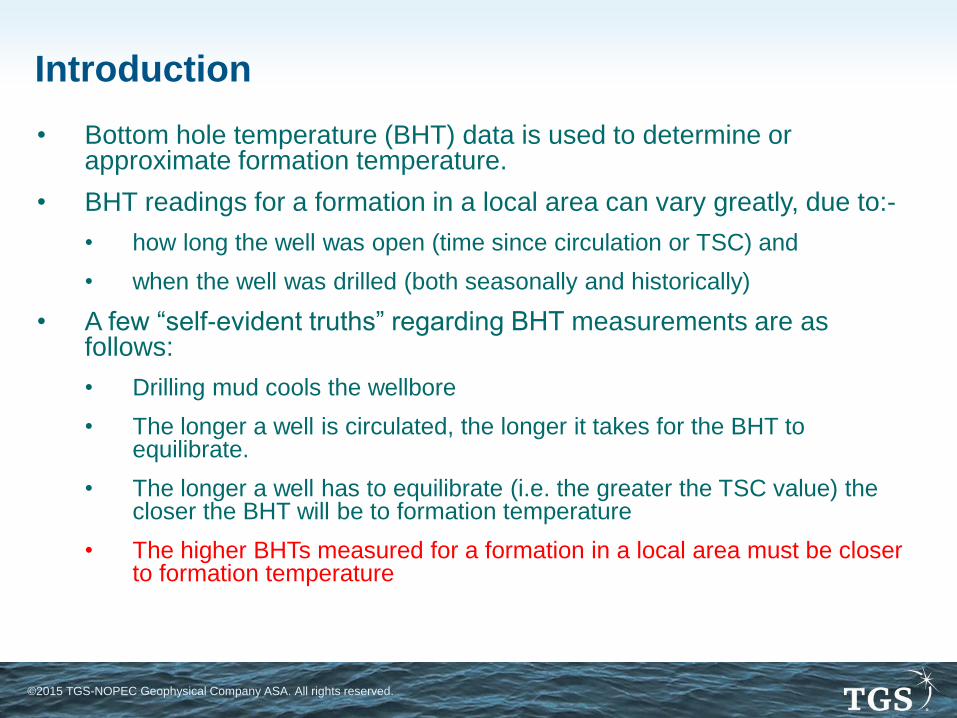
• Bottom hole temperature (BHT) data is used to determine or approximate formation temperature.

• BHT readings for a formation in a local area can vary greatly, due to:-

• how long the well was open (time since circulation or TSC) and

• when the well was drilled (both seasonally and historically)

• A few “self-evident truths” regarding BHT measurements are as follows:

• Drilling mud cools the wellbore

• The longer a well is circulated, the longer it takes for the BHT to equilibrate.

• The longer a well has to equilibrate (i.e. the greater the TSC value) the closer the BHT will be to formation temperature

• The higher BHTs measured for a formation in a local area must be closer to formation temperature

Introduction



• Sprensky (1992 and http://www.sprensky.com/publishd/temper2.html) provides a very succinct summary of the problems and treatments of small to large BHT datasets.

• For small datasets:

• A linear relationship is generally assumed between the ambient surface temperature and uncorrected BHT/depth control points.

• More advanced techniques use measurements of increasing Temperature /TSC pairs, to extrapolate to the temperature at static conditions.

• The most commonly used method is the Horner-type extrapolation of BHT data

• For large datasets, regression techniques have commonly been used to “correct ” BHTs and to calculate geothermal gradients.

Methods of estimating Rock Temperature

from BHT data



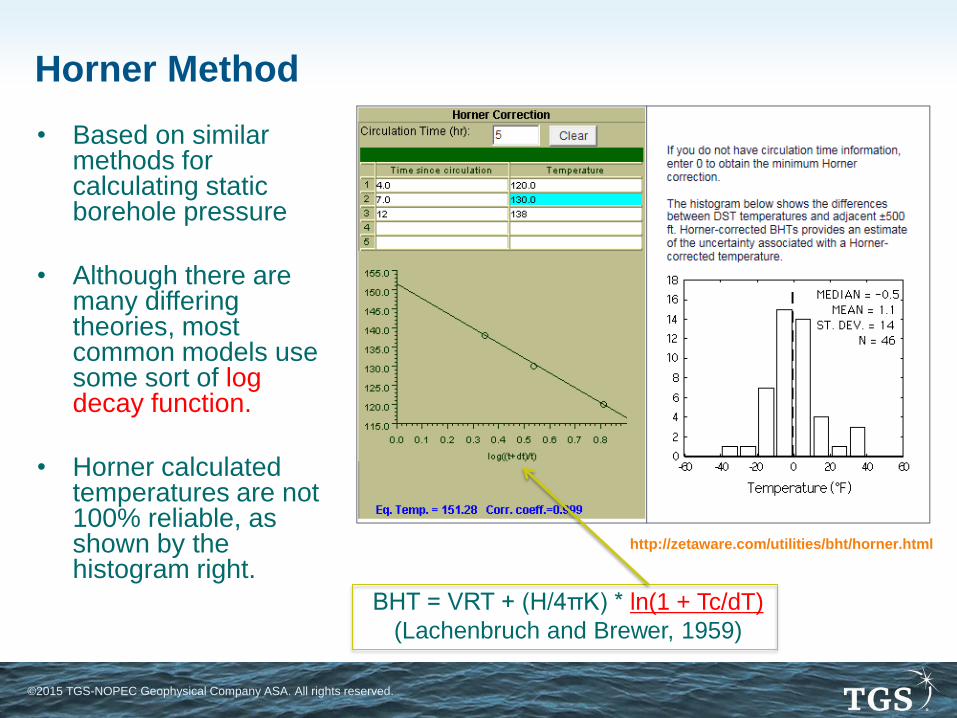
http://zetaware.com/utilities/bht/horner.html

• Based on similar methods for calculating static borehole pressure

• Although there are many differing theories, most common models use some sort of log decay function.

• Horner calculated temperatures are not 100% reliable, as shown by the histogram right.

Horner Method

BHT = VRT + (H/4πK) * ln(1 + Tc/dT)

(Lachenbruch and Brewer, 1959)



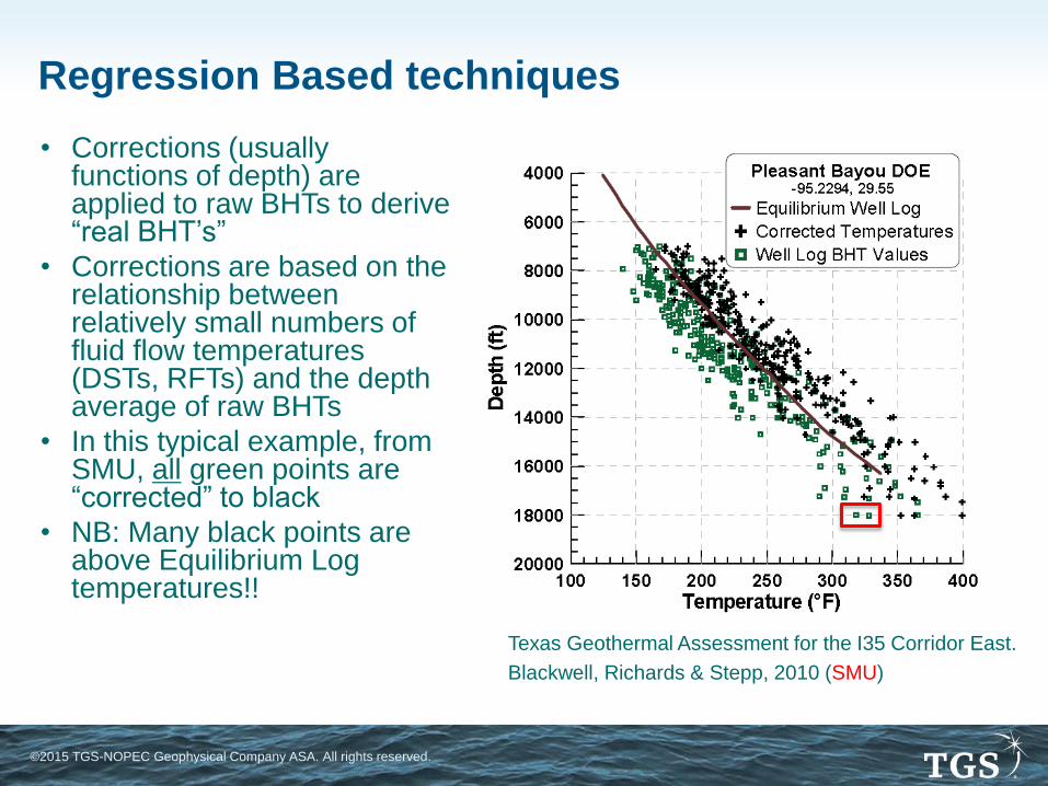
• Corrections (usually functions of depth) are applied to raw BHTs to derive “real BHT’s”

• Corrections are based on the relationship between relatively small numbers of fluid flow temperatures (DSTs, RFTs) and the depth average of raw BHTs

• In this typical example, from SMU, all green points are “corrected” to black

• NB: Many black points are above Equilibrium Log temperatures!!

Texas Geothermal Assessment for the I35 Corridor East.

Blackwell, Richards & Stepp, 2010 (SMU)

Regression Based techniques



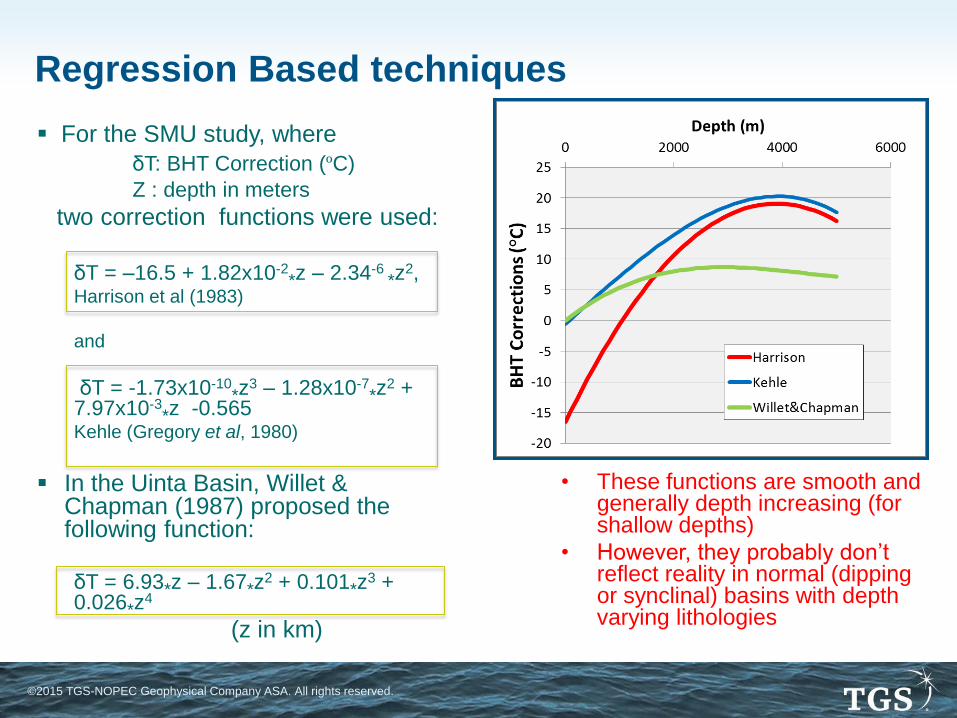
• These functions are smooth and generally depth increasing (for shallow depths)

• However, they probably don’t reflect reality in normal (dipping or synclinal) basins with depth varying lithologies

For the SMU study, where

δT: BHT Correction (ºC)

Z : depth in meters

two correction functions were used:

δT = –16.5 + 1.82x10-2

*z – 2.34-6 *z

2, Harrison et al (1983)

and

δT = -1.73x10-10*z

3 – 1.28x10-7*z

2 + 7.97x10-3

*z -0.565 Kehle (Gregory et al, 1980)

In the Uinta Basin, Willet & Chapman (1987) proposed the following function:

δT = 6.93*z – 1.67*z2 + 0.101*z

3 + 0.026*z

4

(z in km)




• Using the SMU figure we can show three visual trend lines

1. Average raw BHTs

2. Average corrected BHTs (cBHT)

3. Maximum (outer) edge of raw BHTs (MaxG)

• MaxG is very close to the cBHT trend!!

• This coincidence is observed on many similar figures from SMU publications

• Why is this?




• Horner Experiment

• Geothermal Gradient Definitions

• Variation of Interval Geothermal Gradient (IGG) with depth

• The MaxG temperature model

Theory



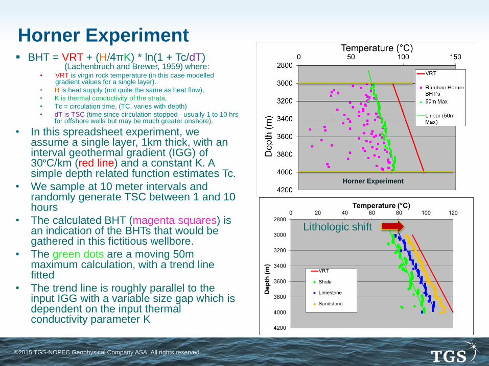
BHT = VRT + (H/4πK) * ln(1 + Tc/dT) (Lachenbruch and Brewer, 1959) where:

• VRT is virgin rock temperature (in this case modelled gradient values for a single layer).

• H is heat supply (not quite the same as heat flow),

• K is thermal conductivity of the strata,

• Tc = circulation time, (TC, varies with depth)

• dT is TSC (time since circulation stopped - usually 1 to 10 hrs for offshore wells but may be much greater onshore).

• In this spreadsheet experiment, we assume a single layer, 1km thick, with an interval geothermal gradient (IGG) of 30ºC/km (red line) and a constant K. A simple depth related function estimates Tc.

• We sample at 10 meter intervals and randomly generate TSC between 1 and 10 hours

• The calculated BHT (magenta squares) is an indication of the BHTs that would be gathered in this fictitious wellbore.

• The green dots are a moving 50m maximum calculation, with a trend line fitted

• The trend line is roughly parallel to the input IGG with a variable size gap which is dependent on the input thermal conductivity parameter K

Horner Experiment

Lithologic shift

Horner Experiment



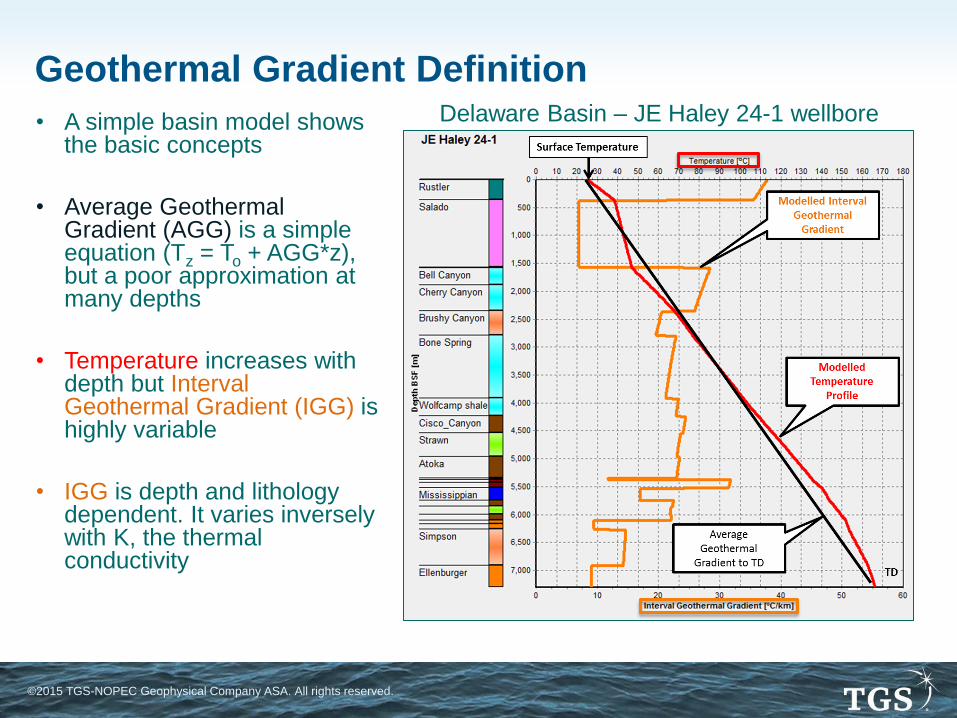
• A simple basin model shows the basic concepts

• Average Geothermal Gradient (AGG) is a simple equation (Tz = To + AGG*z), but a poor approximation at many depths

• Temperature increases with depth but Interval Geothermal Gradient (IGG) is highly variable

• IGG is depth and lithology dependent. It varies inversely with K, the thermal conductivity

Geothermal Gradient Definition Delaware Basin – JE Haley 24-1 wellbore



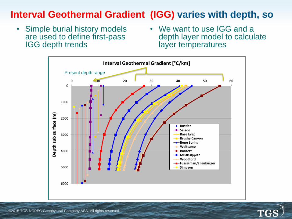
• We want to use IGG and a depth layer model to calculate layer temperatures

• Simple burial history models are used to define first-pass IGG depth trends

Interval Geothermal Gradient (IGG) varies with depth, so

Present depth range



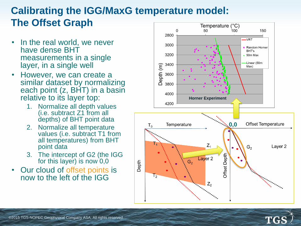
0,0

• In the real world, we never have dense BHT measurements in a single layer, in a single well

• However, we can create a similar dataset by normalizing each point (z, BHT) in a basin relative to its layer top:

1. Normalize all depth values (i.e. subtract Z1 from all depths) of BHT point data

2. Normalize all temperature values (i.e. subtract T1 from all temperatures) from BHT point data

3. The intercept of G2 (the IGG for this layer) is now 0,0

• Our cloud of offset points is now to the left of the IGG

Calibrating the IGG/MaxG temperature model:

The Offset Graph

Horner Experiment



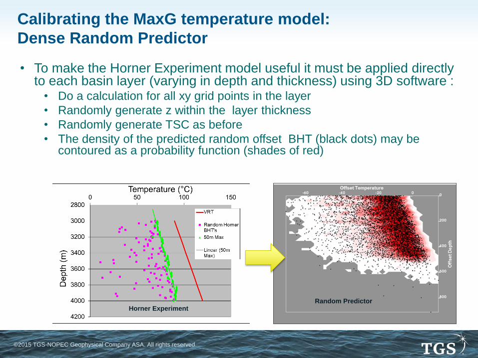
• To make the Horner Experiment model useful it must be applied directly to each basin layer (varying in depth and thickness) using 3D software :

• Do a calculation for all xy grid points in the layer

• Randomly generate z within the layer thickness

• Randomly generate TSC as before

• The density of the predicted random offset BHT (black dots) may be contoured as a probability function (shades of red)

Calibrating the MaxG temperature model:

Dense Random Predictor

Horner Experiment Random Predictor



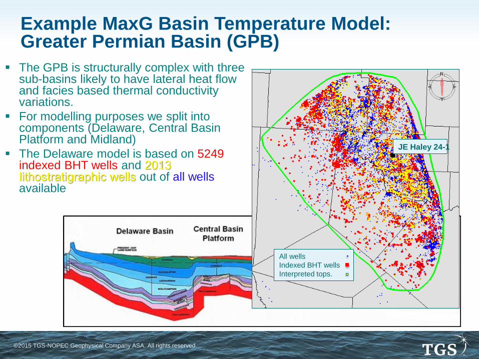
The GPB is structurally complex with three sub-basins likely to have lateral heat flow and facies based thermal conductivity variations.

For modelling purposes we split into components (Delaware, Central Basin Platform and Midland)

The Delaware model is based on 5249 indexed BHT wells and 2013 lithostratigraphic wells out of all wells available

JE Haley 24-1

All wells

Indexed BHT wells

Interpreted tops.

Example MaxG Basin Temperature Model: Greater Permian Basin (GPB)



• We use the layer interpretation to subdivide the

BHTs into layer datasets and produce Offset

Graphs for each layer. This requires 3D software

• Note that the MaxG trend is really a wedge, since

the IGG varies with actual, not offset depth.

• The Wolfcamp Offset Graph compares well with the

random predictor background: a function of

lithologic uniformity. The Bone Springs layer is more

complex

Offset Graph examples

IGG at surface IGG at min depth IGG at max depth

BHT data (white -> brown = deeper

sub surface)

Random Predictor



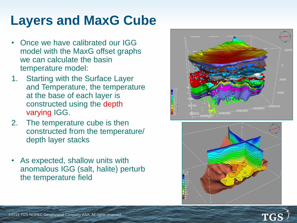
• Once we have calibrated our IGG model with the MaxG offset graphs we can calculate the basin temperature model:

1. Starting with the Surface Layer and Temperature, the temperature at the base of each layer is constructed using the depth varying IGG.

2. The temperature cube is then constructed from the temperature/ depth layer stacks

• As expected, shallow units with anomalous IGG (salt, halite) perturb the temperature field

Layers and MaxG Cube



Finally we merge the three sub-basins to produce the GBP cube

The image here shows three (x,y,z) planes through the cube, which is truncated by the surface layer and the PreC-BMT (deepest layer in the model, shown in white)

Contours are at 10ºF intervals

The MaxG cube is provided as SEGY deliverable

GPB MaxG Temperature Cube

Temperature

ºF



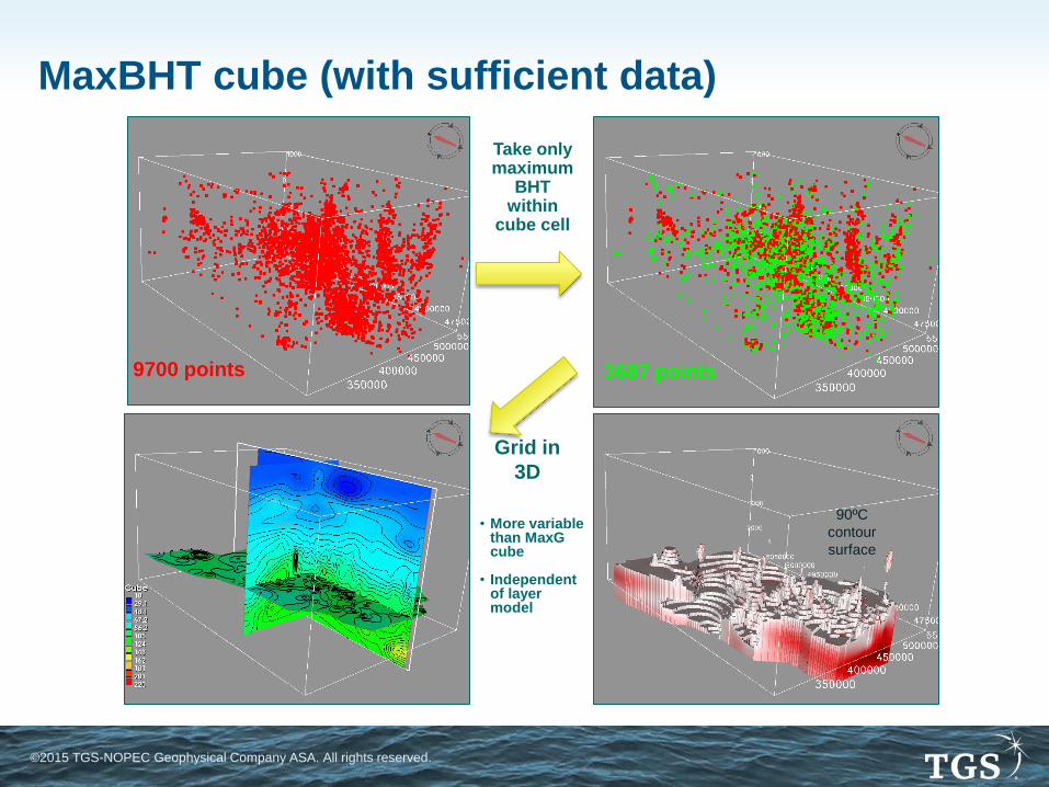
MaxBHT cube (with sufficient data)

9700 points 3687 points

Take only maximum

BHT within

cube cell

Grid in

3D

• More variable than MaxG cube

• Independent

of layer model

90ºC

contour

surface



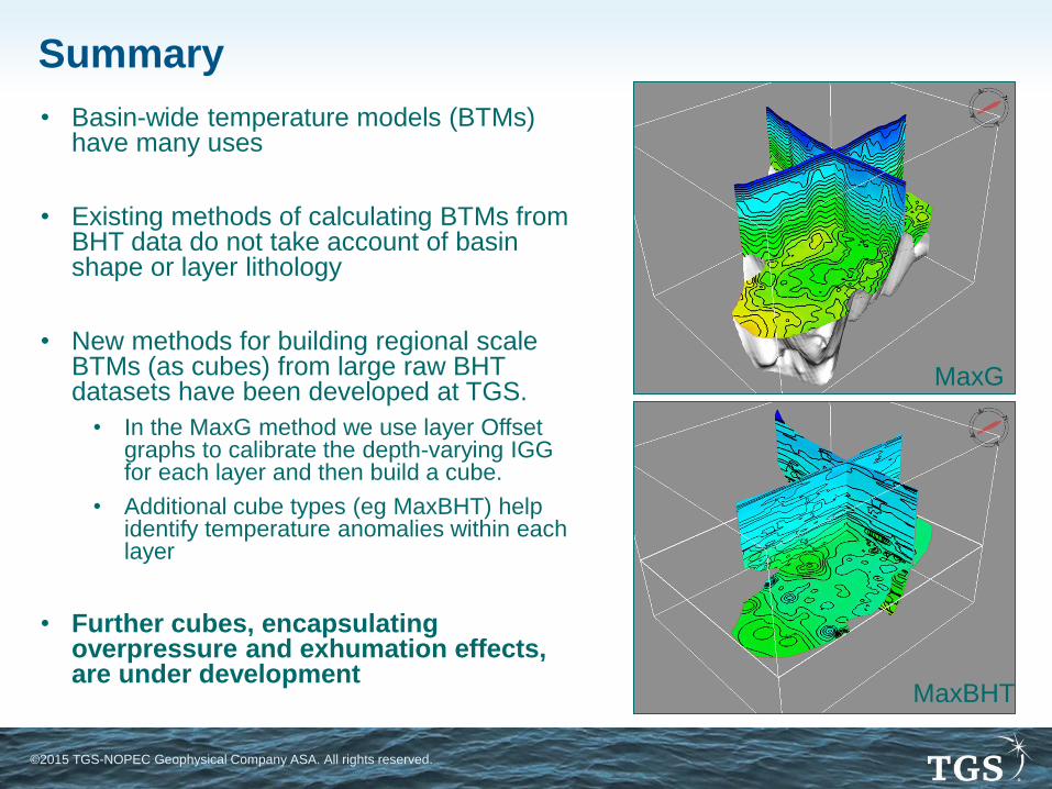
• Basin-wide temperature models (BTMs) have many uses

• Existing methods of calculating BTMs from BHT data do not take account of basin shape or layer lithology

• New methods for building regional scale BTMs (as cubes) from large raw BHT datasets have been developed at TGS.

• In the MaxG method we use layer Offset graphs to calibrate the depth-varying IGG for each layer and then build a cube.

• Additional cube types (eg MaxBHT) help identify temperature anomalies within each layer

• Further cubes, encapsulating overpressure and exhumation effects, are under development

Summary

MaxG

MaxBHT



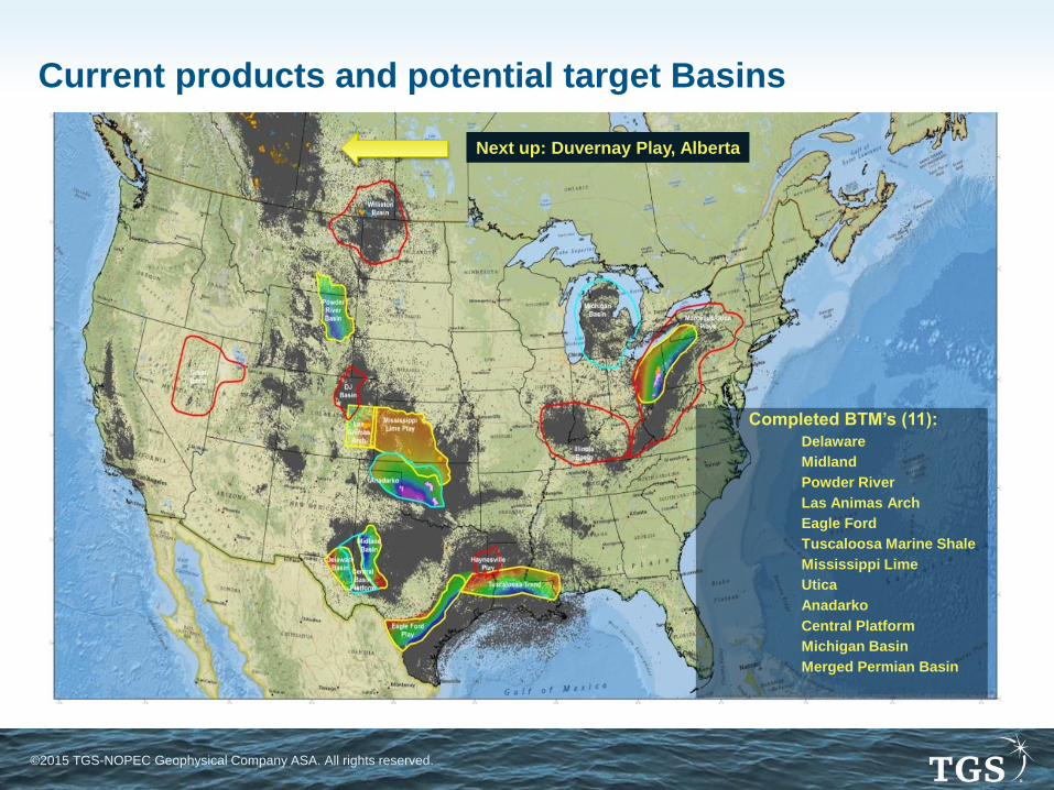
Current products and potential target Basins

Completed BTM’s (11):

Delaware

Midland

Powder River

Las Animas Arch

Eagle Ford

Tuscaloosa Marine Shale

Mississippi Lime

Utica

Anadarko

Central Platform

Michigan Basin

Merged Permian Basin

Next up: Duvernay Play, Alberta

Thank you


Thank you


• TGS for permission to publish

• You for your attention

• Geocap® for continued and timely

software development

[email protected]

[email protected]

mailto:[email protected]

mailto:[email protected]

Date post:	16-Feb-2022
Category:	Documents
Upload:	others
View:	3 times
Download:	0 times

Basin Temperature Modeling using large Bottom Hole ...

Documents