Benchmarking money manager performance:

Issues and evidence

Louis K. C. Chan, Stephen G. Dimmock, and Josef Lakonishok∗

August 2006

∗Chan and Lakonishok are with Department of Finance, College of Business, University of Illinois at Urbana-

Champaign, Champaign, IL 61820; and NBER (Lakonishok). Dimmock is with Department of Finance, Eli Broad

Graduate School of Management, Michigan State University, East Lansing, MI 48824. We thank Kent Daniel, Eugene

Fama, Jason Karceski, Bhaskaran Swaminathan, seminar participants at the Hong Kong University of Science and

Technology, National University of Singapore, Northwestern University Kellogg Hedge Funds conference, University

of Texas Austin for comments, and John Diderich, James Owens, Menno Vermeulen, and Simon Zhang for assistance

with data.

Active money managers offer the allure of returns that exceed market benchmarks. Portfolio managers

with successful track records are highly sought after by investors, while those who fall short of their targets

are eventually fired. Investors’ close scrutiny of a portfolio manager’s performance history highlights the

importance of establishing relevant benchmarks. The research literature provides a variety of procedures.

Earlier studies such as Jensen (1968) use the Capital Asset Pricing Model (CAPM) to generate expected

returns. More recent work draws on Chan, Hamao and Lakonishok (1991), Fama and French (1992), Lakon-

ishok, Shleifer and Vishny (1994), who find that size and the ratio of book-to-market value of equity capture

much of the variation in returns across stocks. The use of these two attributes to measure performance is now

pervasive in academic research, so much so that the Fama-French (1996) three factor model has become the

cornerstone of empirical financial research.

In practice, many investment consultants draw on academic research to develop benchmarks for perfor-

mance evaluation and attribution. Some of the earlier yardsticks, such as the Standard & Poor’s BARRA

indexes until 2005, parallel academic studies in terms of using size and book-to-market as the sole attributes

for stock classification. Other indexes consider additional variables, such as analysts’ long-term growth

forecasts in the case of the Russell indexes. More recently there has been a trend in the industry toward cus-

tomized benchmarks to adjust for investment style along the dimensions of size and value-growth orientation

(see Chan, Chen and Lakonishok (2002)). By identifying a manager’s style, the active portfolio can be paired

with a passive benchmark that mimics the underlying strategy. As a result stock selection skills may come

out more clearly, or the portfolio’s performance can be attributed to various sources.

The upshot is that academic and practitioner research yields a proliferation of methods using size and

value/growth attributes or factors as the basis for benchmarking portfolio performance. At first glance, be-

cause they are variants of the same underlying approach, these methods should be more or less interchange-

able. For example, Fama and French (1992) find that in the cross-section the effect of stocks’ earnings-

to-price ratios is absorbed by size and book-to-market. Additionally, the three-factor model in Fama and

French (1996) captures the returns on portfolios sorted by ratios of earnings or cash flow to price, or sorted

by sales growth. A casual interpretation of these results is that other indicators of a portfolio’s value/growth

orientation are unimportant once book-to-market is accounted for. Similarly, on the surface it may appear

2

that cross-sectional regression methods and time-series factor models yield similar conclusions with respect

to detecting abnormal returns. Perhaps on the basis of this evidence, Fama and French (1993) say that “eval-

uating the performance of a managed portfolio is straightforward” using their three-factor model.

Table 1 follows up on this line of thinking. In particular it examines the notion that different variants of

the size and value/growth benchmarking procedure do not yield serious disagreements about the existence

and level of abnormal returns. We take two benchmarking procedures that are standard in the academic

literature and apply them to evaluate the performance of a sample of 199 institutional money managers (the

full details of the sample and benchmarking procedures are described in the following sections). The first set

of benchmarks comprises reference portfolios that match the size and book-to-market characteristics (as of

the end of June each year) of each stock in a managed portfolio. There are 25 reference portfolios produced

from independent sorts on size and book-to-market. In the second procedure a portfolio’s benchmark return

is the fitted value from the Fama-French (1996) three-factor model time series regression applied to the

entire return history of the managed portfolio. The data on reference portfolio returns as well as on the factor

portfolios are obtained from Kenneth French’s website.

Panel A of Table 1 evaluates long-term performance as measured by mean abnormal returns produced

by the benchmarking procedures. The mean abnormal return is the difference between the annualized geo-

metric mean return of the portfolio and its benchmark return. If the procedures are indeed closely aligned,

for the same portfolio they should deliver average abnormal returns that are of the same sign (over- or under-

performance). Accordingly we report the fraction of managed portfolios where the two methods yield dif-

ferent signs for the mean abnormal return. Also we compare the magnitude of the mean abnormal returns

and report the frequency where their absolute difference exceeds some threshold level. Over the full sample

period of 1989–2001, the methods disagree on the sign of excess return in about one out of four portfolios

(24.62 percent of the cases). The divergence is not confined to a subset of the portfolios. When the com-

parison is carried out across managers who follow the same investment style the frequency of disagreement

varies from 11.11 percent for large growth managers to as much as 50 percent for small growth managers.

As further cause for concern, the mean annualized abnormal returns frequently diverge by large magnitudes.

For the overall sample, the levels of the absolute differences exceed 2.5 percent in 43.22 percent of the cases,

3

and are at least 5 percent in 14.07 percent of the cases. During the volatile period from 1998 to 2000, the

differences are much more pronounced. For instance in this subperiod absolute differences above 5% occur

for 53.85 percent of the small value portfolios, whereas no differences of this magnitude occur over the entire

period.

Investors do not always have the luxury of evaluating performance over long horizons. Rather, decisions

often turn on results over relatively short horizons such as a single quarter or year. Institutional money

managers commonly assess performance relative to a standard index, for example, and issue reports to clients

as frequently as every month. Failure to meet targets invites even more frequent monitoring from clients and

consultants. To capture this short-term orientation, panels B and C of Table 1 repeat the comparisons in terms

of abnormal returns measured over calendar years and over quarters, respectively. In an average calendar year

the matching portfolio and factor model methods produce abnormal returns with divergent signs for 24.49

percent of the managers. When the results are not averaged over a portfolio’s full history, as in panel A,

the extent of the differences are amplified. From panel B, in 65.65 percent of the cases the yearly abnormal

return differs across the methods by at least 2.5%, and differences above 5% occur with a frequency of 41.36

percent. In a given quarter the abnormal returns can also be out of line by large amounts: for the overall

sample absolute deviations in excess of 1% occur with 69.53 percent frequency.

What should one make of these differences in measured performance? One simplistic interpretation is

that they amount to measurement errors and are economically uninteresting. To help assess the materiality of

differences of the magnitude documented in Table 1, we provide some recent evidence on the range in invest-

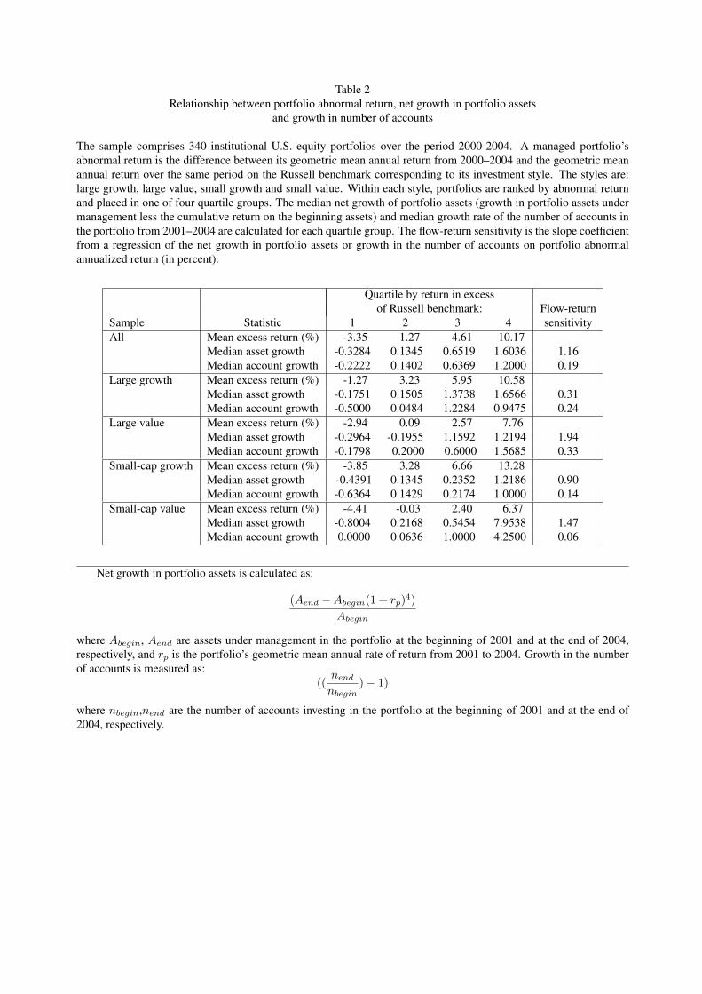
ment performance and its relation with fund flows. Table 2 divides a sample of 340 investment management

firms into categories depending on their prior returns over 2000–2004 in excess of the corresponding Rus-

sell style index. These indexes are the most frequently used yardsticks in the investment industry. We then

see whether, and by how much, differences in performance affect subsequent fund flows into the portfolio.

Fund flows are measured as net growth in assets managed in the portfolio (growth in portfolio assets net of

the gains on the original assets from appreciation). We also look at growth in the number of accounts with

assets invested in the portfolio, another indicator that is less affected by fluctuations in clients’ deposits and

withdrawals. Growth in assets or accounts is measured over the period 2001–2004, leaving a lag of one year

4

between assessing performance results and asset growth. The delay allows time for clients to respond to

performance. We report median growth for the portfolios in each category in order to mitigate the effects of

outliers due to low initial values of assets under management or the number of accounts.

For the entire sample of money managers, the highest-ranked quartile achieved a mean return of 10.17

percent per year above their Russell style benchmark. In contrast the poorest-performing quartile of managers

fell short of their benchmarks by 3.35 percent on average. Managers in the top quartile by prior performance

were able to attract new assets at a median rate of 1.6036 times (over 4 years) of their beginning assets;

the median growth rate of accounts is 120 percent. The median manager in the bottom quartile, however,

suffered an outflow of assets equal to 32.84 percent of original assets and the number of accounts shrank by

22.22 percent. The estimated sensitivity of asset growth to performance from a regression line is 1.16 times,

while each percentage point increase in performance on average is associated with a 19 percent increase in

the number of accounts. Based on these sensitivities, a difference in abnormal return of 2.5 percent translates

into asset flows of 2.9 times original assets, or growth in the number of accounts by 47 percent. The results

from specific styles confirm that performance has a strong association with future growth in portfolio assets

and accounts. The choice of benchmarking procedure can thus have a potentially large impact on manager

rankings, and consequently on their net assets and accounts.

The message from Table 1 is that two seemingly interchangeable benchmarking procedures can produce

very different results with economically important consequences. Other methods for deriving reference port-

folios are widely used as well, so this table is only a first step in gauging how the choice of benchmarking

method affects inferences about investment performance. Our broader objective is to trace the underlying

sources of the differences, identify any potential shortcomings in the procedures and suggest improvements.

To do this we conduct a comprehensive evaluation of the performance of different benchmarks that are based

on stocks’ size and value-growth orientation. In particular our discussion focuses on three broad imple-

mentation issues in benchmark construction. First, we examine the use of independent sorts to determine

size and book-to-market control portfolios. Second, we put the three-factor model up against style-based

return regressions using the full assortment of equity asset classes. Lastly, we analyze how well a portfolio’s

value-growth orientation is captured by looking only at book-to-market.

5

A few other studies, such as Barber and Lyon (1997), Fama (1998), Lyon, Barber and Tsai (1999),

Mitchell and Stafford (2000) alert researchers to the hazards of testing for abnormal returns in long-term

multi-year event studies. Table 1 suggests, however, that it is no less perilous to benchmark performance

in a context that may appear to be fairly standard and well-understood, namely, the evaluation of portfolio

performance over relatively short horizons. This paper provides such caveats and proposes some remedies.

We apply the benchmarking procedures to two sets of data. To ensure that our test environment captures

all the conditions that would exist in a typical evaluation or attribution exercise, we analyze the returns

from a sample of large institutional money managers over the 1989–2001 period. We provide comparisons

across methods averaged over managers, as well as comparisons of how individual managers are ranked.

Additionally, we take the methods to the returns on passive indexes whose composition follows clearly pre-

specified criteria. Different evaluation methods are more likely to agree on average over long time periods and

during more tranquil market conditions. However, investment decisions are often made over short timeframes

and under turbulent conditions. To accommodate these considerations, we break out the results for the 1998–

2000 subperiod. The cross-sectional variation in returns across different equity asset classes peaked in the

late 1990s (see Chan, Karceski and Lakonishok (2000)), so this period presents a particularly interesting

stress test of performance evaluation methodologies.

Our evidence on the performance of money management firms that invest equity assets of institutional

clients is also of independent interest. In the U.S., institutional investors account for a sizeable proportion

of the ownership of listed equities. In 2003, for example, they held $8 trillion of U.S. corporate equities,

or about 59.2 percent of the value of publicly traded equity (Brancato and Rabimov (2005)). One set of

institutional investors, mutual funds and closed-end funds, has commanded the bulk of attention from the

popular press and academic studies. An extensive literature studies the performance of equity mutual funds.

An incomplete list of studies includes Elton, Gruber, Das and Hlavka (1993), Malkiel (1995), Gruber (1996),

Daniel, Grinblatt, Titman and Wermers (1997), Carhart (1997), and Kothari and Warner (2001).

At the same time, another group of institutional investors, namely managers of the equity assets of pen-

sion funds, endowments and foundations, has been much less studied. This is despite the fact that, in terms of

stock holdings, pension plan money managers are much more important than mutual and closed-end funds.

6

Of institutionally-owned U.S. equity assets in 2003, 41 percent was held by pension funds while 22 per-

cent was held by mutual and closed-end funds. There are, however, far fewer studies on the performance

of pension plan money managers (see Lakonishok, Shleifer and Vishny (1992), Coggin, Fabozzi and Rah-

man (1993)). This study provides some new results on this important, but generally overlooked, segment of

professional investors.

The evidence in this paper has implications beyond our focus on the evaluation of managed portfolios’

performance. Any analysis of long-term stock price performance invariably has to grapple with the choice of

an appropriate benchmark for comparison. The issue is central in studies of stock market efficiency, such as

tests of the profitability of trading strategies. Research in corporate finance that examines the impact of var-

ious managerial decisions, such as equity offerings, dividend initiations or omissions, and share repurchase

programs, also faces the problem of measuring stock returns in excess of some normal level.

Our key result is that judgments about the magnitude of performance are sensitive to benchmarking

methodology. To illustrate, mean abnormal returns are 2.64 percent relative to the Fama-French three-factor

model, 1.39 percent when compared to reference portfolios based on independent sorts on size and book-

to-market, a measly 0.78 percent when we use a more comprehensive measure of value/growth, and drop to

-1.97 percent relative to a benchmark from cross-sectional regressions of returns on stock attributes. These

differences stand out all the more because they are averages across an extensive sample of portfolios over

many quarters. Inferences about performance are fragile despite the fact that our procedures all rest on the

same basic premise that a portfolio’s size and value/growth orientation are central determinants of its expected

return. To sharpen this point, in practice performance tracking and attribution analysis often employs models

with many factors over short periods. In light of the difficulty of filtering out managerial skill from investment

style, such exercises may rest on shaky grounds.

Tracking error volatilities provide a way to judge how well the benchmarks capture the behavior of active

portfolios. In this respect benchmarks from procedures that are widely used in academic research disappoint,

yielding high tracking error variability. We trace their relatively poor showing to underlying methodologi-

cal drawbacks — independently sorting stocks by size and book-to-market, treating the effects of size and

value/growth as linear additive terms that are uniform across all stocks, and relying on book-to-market as the

7

sole yardstick for value/growth classification. Conversely, methods that bypass these shortcomings, such as

forming control portfolios by two-way sorts on size and then on a comprehensive indicator of value/growth

orientation, do well in terms of producing relatively low tracking error volatility. To illustrate the point, out-

of-sample tracking error volatilities average 10.54 percent under the conventional three-factor model, while

dollar-weighted reference portfolios that match the size- and composite value characteristics of active man-

agers deliver mean volatilities of 8.71 percent. More generally, evidence from the Russell indexes, which are

passive portfolios with stable makeup, indicates that characteristic-matched benchmarking procedures have

better tracking ability than regression-based procedures.

The remainder of the paper is organized as follows. Section 1 describes our data and outlines some key

choices with respect to benchmark construction. To streamline the discussion we discuss separately bench-

marking procedures that are based on portfolio holdings and those based on return regressions. Section 2 of

the paper provides results on investment performance based on characteristic-matched baseline portfolios.

To provide a deeper exploration of the sources of the differences across benchmarking procedures, Section 3

applies them to passive portfolios as measured by the Russell style indexes. Further we provide details on the

characteristics of the benchmark portfolios. Results on money manager performance relative to regression-

based benchmarks are provided in section 4. Some diagnostics on how the regression-based benchmarks

fare, including its performance on passive indexes, are contained in section 5. Section 6 takes up the issue

of how the results for a managed portfolio vary with the choice of benchmarking procedure. A final section

concludes.

1 Preliminaries

1.1 Data

Our sample describes the returns and holdings every quarter from 1989Q1–2001Q4 of 199 U.S. institutional

equity portfolios offered by investment management firms. These portfolios span a variety of styles in terms

of size and value-growth orientation. While the portfolios vary in terms of when their return histories start

and end, we require that each has at least 16 consecutive quarters of returns. The data are collected by SEI

8

Investments, a large investment services firm.

The data set is not entirely free of selection bias: larger, relatively more successful managers are more

likely to be covered by the database. Nonetheless, it is representative of performance databases that are

maintained by investment consulting firms, and which are widely used in clients’ searches for portfolio

managers. Compared to prior studies of pension fund equity portfolios, such as Coggin et al. (1993), we

observe, in addition to the returns on the portfolios, the composition of the portfolio in terms of the amounts

invested in each stock at the beginning of a quarter.

1.2 Issues in benchmark construction

Each of our benchmarking procedures translates observable stock characteristics or factor loadings into a re-

turn that is expected on the managed portfolio. The aim in so doing is to disentangle the manager’s skill from

luck. We examine two variants of this benchmarking methodology, each of which is widely employed. In one

variant, benchmark returns are obtained from attribute-sorted portfolios that match the features of the stocks

held by the active manager. Daniel, Grinblatt, Titman and Wermers (1997) apply this “characteristic-based”

approach to study the performance of U.S. equity mutual funds. In the other variant, the benchmark returns

are obtained from regressions of the managed portfolio’s returns on the market and other zero investment

factor-mimicking portfolios. Carhart (1997) is one example of this second, “regression-based” approach to

performance measurement.

However, there is a wide variety of ways to construct benchmark returns, even when we restrict attention

to size and value/growth as the main dimensions that capture the behavior of stock returns. In broad terms,

the choices involve: the use of stock attributes or loadings from regression models; the specific measures of

value/growth orientation; whether size and value/growth are treated independently; the weighting scheme for

stocks in the benchmark; and the frequency with which the benchmark’s composition is updated.

1.2.1 Attributes or loadings

The first set of procedures uses stock attributes as predictors of a managed portfolio’s return. This is done by

pairing each holding in the active portfolio with a reference portfolio that mimics as closely as possible the

9

stock’s size and value/growth tilt. The weighted average of the matching portfolios’ returns over all holdings

yields the benchmark return for the active portfolio. Instead of using reference portfolios, the return can be

predicted from a cross-sectional regression of stock returns on beginning-of-quarter stock attributes.1

Daniel and Titman (1997) find that stock attributes do a better job than factor loadings in predicting the

cross-section of returns. However, timely data on managers’ portfolio holdings are not generally available so

many studies estimate expected returns with factor loadings from time series return regressions.

1.2.2 Measuring value/growth style

In many studies a stock is considered as value or growth solely on the basis of its book-to-market ratio.2

Similarly, factor loadings with respect to a zero-investment mimicking portfolio that is long (short) in stocks

with high (low) book-to-market ratios are used to assign stocks to value or growth categories. As Lakonishok,

Shleifer and Vishny (1994) note, however, the ratio of book-to-market value of equity is an incomplete mea-

sure of a stock’s value-growth orientation. For example, under current U.S. accounting standards book values

do not include the value of intangible capital such as investments in research and development (see Chan,

Lakonishok and Sougiannis (2001)). Similarly measured book values currently ignore the underfunding of

companies’ pension liabilities. Looking at other indicators such as earnings, dividends or sales may help to

paint a clearer picture of a stock’s value-growth stance.

1.2.3 Independence of size and value/growth classification

Many studies form reference portfolios by two-way sorts on size and book-to-market equity. A crucial issue

here is whether the sorts are done independently, or within a particular group. In one-way sorts by book-

to-market, the growth (low book-to-market) category tends to comprise larger stocks than the value (high

book-to-market) category. Intersecting this classification with an independent sort by size thus results in

large stocks generally being clustered in the growth category. The problem is that this classification provides

1The Barra performance attribution system, which is heavily used in the investment industry, is based on such a cross-sectional

regression approach.2The academic research literature generally has not addressed issues related to the measurement of size. While market capital-

ization is one choice, adjustments for cross-holdings or privately-held shares present other possibilities.

10

a poor depiction of money managers’ investment domains. Many investment managers tend to concentrate

on larger stocks, where information as well as liquidity tends to be more available. Within the category of

large stocks, some managers who are more value-oriented seek out comparatively cheap, undervalued stocks

that have attractive earnings or dividend yields. Other large-capitalization managers who are more glamour-

oriented seek out stocks with high growth potential, or substantial investments in intangible capital. Despite

the differences in their approaches, an independent classification scheme might hold both groups of managers

to similar benchmarks (large stocks with low book-to-market ratios).

An alternative to the classification scheme based on independent sorts is to define value and growth within

each size category. This corresponds more closely to how portfolio managers structure their stock selection

process, whereby a manager may choose, for example, relatively cheaper stocks within mid-sized firms. As

evidence of the pervasiveness of this practice many widely-used market indexes, such as those produced by

the Frank Russell Company, S&P Citigroup, and Wilshire Associates, follow the approach of defining value

or growth within groups of similarly sized firms.

1.2.4 Weighting scheme

A benchmark is intended to capture the performance of a representative set of stocks that share similar fea-

tures. It is thus undesirable if the benchmark’s behavior is driven by a relatively small subset of the underlying

stocks. In many empirical studies, for example, returns are measured against a portfolio comprising equal

dollar amounts invested in a group of comparable stocks. The equal weighting prevents the behavior of the

yardstick from being dominated by idiosyncratic shocks to a few stocks. However this tends to give rela-

tively more weight to smaller stocks in the benchmark. Value-weighting the component stocks, on the other

hand, tends to emphasize larger stocks whose returns are generally less noisy. Further, biases in computing

expected returns that are induced by rebalancing are mitigated by value-weighting.

1.2.5 Frequency of reconstitution

A stock’s attributes may change over time, so that a reference portfolio that originally represents stocks with

similar features may become less homogenous. The ability of the reference portfolio to track the active

11

portfolio’s return may thus deteriorate over time. Reconstituting the reference portfolio more frequently

alleviates the problem. Suppliers of benchmark indexes, for example, update their indexes every quarter

(Wilshire) or once a year (Russell).

Since our collective understanding of the return generating process is incomplete, it is important to ensure

that the performance results do not hinge upon the choice of a benchmarking model. Accordingly, in our

evaluation of money manager performance in the subsequent sections, we employ an assortment of methods

that represent different choices with respect to each of the considerations above.

2 Performance relative to characteristic-matched portfolios

We discuss performance relative to characteristic-matched benchmarks using portfolio holdings in this sec-

tion. The analysis of performance under regression-based benchmarks is deferred to the next section.

2.1 Methods

We use four versions of characteristic-matched reference portfolios. In every case the benchmark for a given

managed portfolio is constructed as follows. Each stock in the managed portfolio, based on its size and

value/growth attribute ranks, is paired with one of the reference portfolios. The benchmark return is then

the weighted average of the buy-and-hold quarterly returns of the control portfolios, using the investment

weights of the manager as of the beginning of the quarter.

2.1.1 Independent size, book-to-market sorts

In the first procedure we use independent sorts to form reference portfolios for each size and value/growth

category. This procedure mirrors the method of Fama and French (1996) and other studies (Ikenberry, Lakon-

ishok and Vermaelen (1995), Brav and Gompers (1997), Daniel, Grinblatt, Titman and Wermers (1997),

Lakonishok and Lee (2001), Chan, Lakonishok and Sougiannis (2001)). The control portfolios are formed

once a year in July. The sort on size (the market value of common equity of the stock as of the end of June)

yields five portfolios based on NYSE breakpoints. Independently, stocks are ranked and sorted into quintile

12

portfolios by the ratio of book to market value of common equity (also based on NYSE breakpoints). Book

value is from the latest fiscal year ending in the prior calendar year, while market value is from December

of the previous year-end. The intersection of these two sorts yields 25 control portfolios. The return on

each portfolio is either the equally-weighted or value-weighted average of the buy-and-hold returns on the

component stocks.

2.1.2 Size, conditional book-to-market sorts

Alternatively we partition stocks into value and growth categories for similarly-sized firms as follows. At

the end of June each year we define six categories of firms by size (market value of equity), moving down

from the largest to the smallest stock in the listed U.S. domestic common equity universe. The categories are

defined such that each represents a meaningful share of market capitalization, while still comprising a fairly

large number of firms. The first group is made up of the top 75 stocks by market capitalization, while the

second includes the next 125 largest, then the next 300 largest make up the third, the following 500 stocks

are placed in the fourth, the next 1000 stocks in order of size are in the fifth, and the remainder make up the

last group.3 Within each size category, we rank stocks by the ratio of book value of equity (as of the prior

fiscal year) to market value of equity (as of December in the prior year) and classify them from relatively

value-oriented to relatively growth-oriented (with high or low book-to-market ratios, respectively). Since the

first category by firm size (the largest 75 stocks) contains a relatively small number of stocks it is divided into

only three groups (with an equal number of stocks in each group) by value/growth; within each of the other

size classifications there are five groups by value/growth, with roughly equal numbers of stocks.4 There is a

total of 28 portfolios under this size, conditional book-to-market classification scheme. Within each portfolio

the buy-and-hold returns on the component stocks are either equally-weighted or value-weighted.

3The largest 75 stocks make up on average 45 percent of total equity market capitalization, while the other groups represent on

average 20 percent, 15 percent, 10 percent, 6 percent and 4 percent respectively.4An alternative method is to divide each size class into value/growth subsets with roughly equal market capitalization, as is done

in many indexes used by the investment community. To provide a more direct comparison with benchmarking methods used in

academic research, however, we do not follow this approach.

13

2.1.3 Size, composite conditional value/growth indicator approach

Our third approach does not rely solely on book-to-market as the indicator of value/growth; moreover a

stock’s value/growth orientation is defined relative to similarly-sized firms. Specifically, we construct a

composite indicator variable to measure value/growth orientation. The composite is the rescaled average of

a stock’s percentile rank on each of five attributes, such that the most value-oriented (growth-oriented) stock

within a given size category receives a rank of one (zero). The five characteristics are: book-to-market ratio;

sales to price ratio; cash flow to firm value; dividend yield; and earnings yield. Once ranks are calculated

over as many of these variables as are available, the simple average is computed.5 Stocks within a given size

category are then ordered by this average from lowest to highest and the final composite indicator for thei-th

ranked stock isi−1n−1 , if there aren stocks in the size category. The return on the reference portfolio is either

an equally-weighted or value-weighted average of the underlying stocks’ returns.

2.1.4 Quarterly size, conditional book-to-market sorts

In the above three procedures, the control portfolios are updated once a year at the end of June. Using

stale data may mean that a reference portfolio’s underlying characteristics (hence its expected return) are not

fully aligned with the active portfolio. To allow a closer correspondence, our fourth procedure uses size,

conditional book-to-market matched portfolios where the control’s composition is updated every quarter

using current quarter-end market capitalization. As with the other methods, we report both equally-weighted

and value-weighted returns.

5Characteristics are calculated in July each year. Values for accounting variables are taken from the latest fiscal year as of the

prior year-end, and are scaled by stock price or market capitalization in December of the previous calendar year. Sales-to-price is

net sales divided by equity market capitalization. Cash flow to firm value is operating income before depreciation divided by firm

value (total assets less book value of common equity, minus accounts payable, plus market value of common equity). Dividend

yield is cash dividends to common equity divided by equity market capitalization. Earnings yield is income before extraordinary

items available to common equity divided by equity market capitalization. Negative values for the accounting variables are treated

as follows. As in Fama and French, stocks with negative book values of equity are excluded from the analysis. Cases with negative

values for net sales, cash flow or earnings, and firms not paying dividends, are assigned ranks of zero for the respective variable. The

remaining cases with nonnegative values or positive dividends are ranked from lowest to highest.

14

2.1.5 Russell style indexes

Finally, as a baseline comparison for our reference portfolios, we use the Russell style indexes. In practice

these are the most commonly used benchmarks for institutional equity investors. Specifically, we estimate

the manager’s style and, on this basis, assign a corresponding Russell style index to the active portfolio.

Chan, Chen and Lakonishok (2002) find that mutual fund portfolios’ attributes provide good guidance on

their investment styles. We follow their approach and use the size and composite value indicator variables as

style descriptors. Specifically, a portfolio’s weighted average size percentile rank (one for the largest stock

and zero for the smallest stock) across its holdings determines the manager’s size orientation. Size ranks

above 0.8 are classified as large; size ranks between 0.8 and 0.6 are classified as midcap; size ranks below

0.6 are treated as small. A manager’s composite value score (one for the most value-oriented and zero for the

most growth-oriented) determines the value/growth orientation. Indicator values above 0.67 denote value;

those below 0.33 denote growth; the intermediate range is classified as “neutral”.6 Large, midcap and small

capitalization value or growth managers are paired with the appropriate Russell 1000, Russell mid-cap and

Russell 2000 value or growth index. Neutral portfolios are compared against the corresponding Russell size

benchmark.

2.2 Results

In accord with standard practice in the investment management industry a portfolio’s average abnormal return

is its time-series geometric mean annual return minus the time-series geometric mean annual return on the

matched benchmark. In the absence of any stock selection ability the average abnormal return should be

close to zero. While a reference portfolio may be unbiased in the sense that on average it yields the same

return as an active portfolio, it may nonetheless fail to track the managed portfolio’s return closely. As a

result the control procedure may yield unreliable inferences about performance. Everything else equal, a

6Chan, Chen and Lakonishok (2002) find that while a mutual fund portfolio’s characteristics reliably predict its investment style,

the fund’s returns also provide information. Accordingly, we override the style classification based on portfolio characteristics if

the behavior of the managed portfolio’s returns generates a conflicting signal about its style. In particular, we examine the managed

portfolio’s loadings on the Wilshire style indexes. If, for example, a manager is classified as value based on the multiple indicator

approach but the portfolio also loads heavily on the Wilshire growth indexes, then the manager is assigned to the neutral category.

15

benchmark that tracks better the active portfolio raises the confidence that any differential performance on

the part of the manager is due to skill rather than luck. Accordingly we also examine tracking error volatility

under each of the methods, defined as the annualized standard deviation of the quarterly differences between

the portfolio’s return and the benchmark’s return. To the extent that the benchmark portfolio aligns with the

manager’s investment domain, the tracking error volatility should be low.

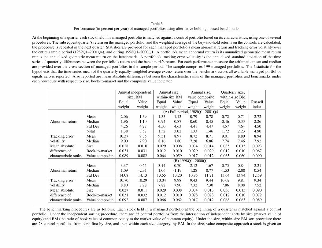
Table 3 summarizes the distribution of abnormal return and tracking error volatility across the sample of

money managers for each method. The cross-sectional average and median are reported for the entire sample

period and also for the 1998Q1–2000Q1 subperiod.

The procedures in Table 3 share the same underlying viewpoint about what drives stock returns. More-

over the results are averaged across a broad sample of portfolios over many years. The presumption therefore

is that any differences across the methods should be meager. This is not the picture that emerges from Table

3. The striking aspect, rather, is that the level of excess returns varies markedly across methods. Compar-

ing across all the methods, abnormal returns range from a high of 2.72 percent to a low of 0.71 percent

for the overall sample period, yielding a range of 2.01 percent. Median abnormal returns display a similar

range across the methods. Put another way, what might appear to be slight variations of the same underlying

methodological approach translate into quite different conclusions about the level of performance.

Notably, the largest abnormal return, 2.72 percent, arises when the Russell indexes are used as the bench-

mark. The equally-weighted portfolio of managers earns a mean quarterly abnormal return that is 4.90

standard errors away from zero.7 Hence, generic indexes that have a wide following in the investment indus-

try suggest reliably high levels of performance for this set of managers. This finding probably reflects the

selection bias underlying the sample: many databases that are used in the investment industry to track perfor-

7To the extent that managers follow similar strategies and pick some of the same stocks abnormal returns will be cross-sectionally

correlated. As a result significance tests based on the cross-sectional standard deviation are misleading. To get around this corre-

lation, we work with the return on an equally-weighted portfolio of all money managers in the sample in the quarter. The standard

deviation of the portfolio return builds in the cross-sectional correlation, and lets us check whether the average return is significantly

different from zero relative to its time series volatility. When we test for the equality of mean abnormal returns across the procedures

in Table 3 for this equal-weighted portfolio of managers, the F-statistic (with standard errors adjusted for clustering by time) is 2.89

with a p-value of 0.01.

16

mance, such as the one we use here, are designed to aid in selecting superior managers. Since performance in

practice is usually measured against the Russell benchmarks, the managers that are followed are more likely

to be the ones who stand out against the Russell style indexes.

Tracking error volatilities indicate how well the benchmark return series from each procedure covary with

the portfolio returns. Reference portfolios from independent sorts yield the highest tracking error volatilities

on average. Equally-weighted benchmarks under this procedure generate a mean tracking error volatility of

10.37 percent per year. Given the lower variability in the returns on large stocks, and the stronger covariation

between large stocks, the tracking error volatility is reduced to 9.35 percent when the control portfolios are

value-weighted. In comparison, when we use a finer size classification and measure book-to-market ranks

within similarly-sized firms, tracking error volatilities drop to 9.51 percent (8.97 percent) for the equal-

weighted (value-weighted) portfolios. A more comprehensive measure of value/growth orientation lowers

the tracking error volatility further to 8.7 percent.8

The active portfolios are concentrated stock groupings with a changing makeup, and whose returns con-

tain a relatively high idiosyncratic component. They therefore provide tough challenges to track, so the

benchmarking procedures all tend to be fairly closely clustered in terms of their tracking error volatilities.

Chan, Karceski and Lakonishok (1999) provide additional perspective. They construct portfolios that are op-

timized under a tracking error variance criterion, and examine how the results change as they apply different

models to forecast return covariance matrices. The data suggest that models with varying degrees of com-

plexity do not produce large differences in realized tracking error volatility out-of-sample. When applied to

random samples of firms, going from the simplest model based on a single market factor to a detailed model

using 9 factors for predicting covariances leads to a reduction of only 1.11 percent per year on average. This

is roughly comparable to the range in tracking error volatilities across the methods in Table 3 for active

8One interpretation of the benefit from reduced tracking error volatility is as follows. Consider the sample size, in years, required

to declare an abnormal annual return of 4 percent to be reliably nonzero at the ten percent significance level. This is roughly( 1.64σ4

)2

whereσ is the tracking error volatility. Forσ of 10.37 percent from independently sorted control portfolios, for example, the required

sample size is 18 years, compared to 13 years if the tracking volatility is 8.71 percent. In other words, the procedure with higher

tracking volatility suffers an efficiency loss of 38 percent relative to the procedure with lower volatility.

17

portfolios. The conclusion is that the differences across methods in tracking error volatilities is material.9

As an aid in identifying the sources of the differences between methods’ tracking error volatilities, Table

3 also reports how the features of an active portfolio match up with the characteristics of the benchmarks.

For each stock in a portfolio its rank on either size, book-to-market or its composite value score is compared

with the corresponding rank of its matching reference portfolio.10 We calculate the simple mean of the

absolute differences of these ranks across all stocks in the portfolio. For instance, when compared to equally-

weighted reference portfolios from independent sorts on size and book-to-market, the average managed fund

has a mean absolute difference in size rank from its benchmark of 0.028.

Contrasting value-weighted and equal-weighted versions of the benchmarks indicates that the former

have an edge in matching the active portfolios’ attribute ranks. The reduced differences help account for the

lower tracking error volatilities produced by value-weighted reference portfolios. Looking across procedures,

the methods all perform comparably in terms of resembling the size and book-to-market features of the

managers’ portfolios. However mean absolute differences with respect to the composite value indicator yield

larger deviations. These contrasts tend to line up with the methods’ tracking error volatilities. Equally-

weighted benchmarks from independent sorts generate absolute differences on average of 0.089 and tracking

error volatility on average of 10.37 percent. For equally-weighted benchmarks matched on size and the

composite indicator the mean absolute difference is 0.017 and the tracking error volatility is 8.72 percent.

The implication is that the procedure of matching portfolios only on size and book-to-market characteristics,

which is customary in many academic studies, may overlook important sources of predictable variation in

returns.

Nevertheless, even the size and value composite approach does not do much better then the Russell

indexes with respect to tracking error. The latter method gives a tracking error volatility of 8.94 percent on

9We can reject at the ten percent significance level the hypothesis that tracking error variances are identical across the methods

in Table 3. The F-statistic is 1.90, with a p-value of 0.08.10Ranks are calculated for all domestic common equities with coverage on the CRSP and Compustat databases. In July of each

year stocks are ordered and assigned ranks from zero (for the stock with the lowest value of the attribute) to one (for the stock with

the highest value of the attribute). Similarly a reference portfolio’s attribute rank is the weighted average rank of its component

stocks, with weights given by the beginning-of-period portfolio proportions.

18

average, despite the large mean absolute differences with respect to the portfolio characteristics. The Russell

indexes are value-weighted portfolios with low volatility. Book-to-market ratios are supplemented with long-

term growth rate forecasts to assign stocks within a size category to value and growth subsets. These features

of the Russell benchmarks may partly account for their relatively strong showing. Additionally, since the

Russell indexes are so widely used in practice for evaluation purposes many managers constrain themselves

from being too out of line with respect to these benchmarks. For example, they may try to limit how far their

portfolio weights deviate from the index weights, and they may try to stay close to the industry composition

of the index. Note also that the indexes are based on relatively coarse breakdowns by size and value-growth

orientation: for example, stocks within a size category (such as the largest 1000 stocks) are partitioned into

only two groups (value and growth) so that they have roughly the same total market capitalization. As a

result the deviations with respect to characteristics can be sizeable.

Managers’ track records diverge markedly during the 1998Q1–2000Q1 subperiod (panel (B)).11 As an

illustration of how differences in the return behavior of equity asset classes were amplified during this period,

in the case of independently sorted reference portfolios equally-weighted benchmarks yield mean abnormal

returns of 3.37 percent. Value-weighted versions of the same benchmarks generate mean abnormal returns

of 0.65 percent.

Comparisons of tracking error volatilities in the later subperiod do not materially change the earlier

conclusions from panel (A). Tracking errors are largest under the independent sort procedure (10.70 percent

for equally-weighted portfolios) and lowest when the benchmarks are the Russell indexes (9.34 percent).

Value-weighted benchmarks based on size and the composite value indicator generate an average tracking

error (9.44 percent) that is close to that of the Russell benchmark.12

11The cross-sectional standard deviation of abnormal returns during this subperiod range from about 11 to 14 percent across the

methods. By comparison, the standard deviations for the overall period are only about 4.5 percent.12Comparing tracking error volatilities between the overall period (panel A) and the 1998–2000Q1 subperiod (panel B) indicates

little signs of change. This is misleading, however, because the overall period extends from the early 1990s when the investment

industry generally was less concerned about tracking indexes. There is a decline in the overall level of tracking error volatility until

the late 1990s when it jumps up. In the 1995–1997 period immediately preceding the subperiod in panel B, for example, tracking

error volatilities for the sample average 6.58 percent across methods.

19

In summary, reference portfolios generated from different versions of the same methodology based on

matching size and value/growth attributes deliver quite different verdicts about the performance of money

managers. Benchmarks derived from independent sorts by size and book-to-market fare particularly poorly

in terms of tracking active portfolio returns. A method that uses a finer partitioning of stocks into size

brackets, and a more comprehensive measure of value/growth orientation delivers lower tracking errors.

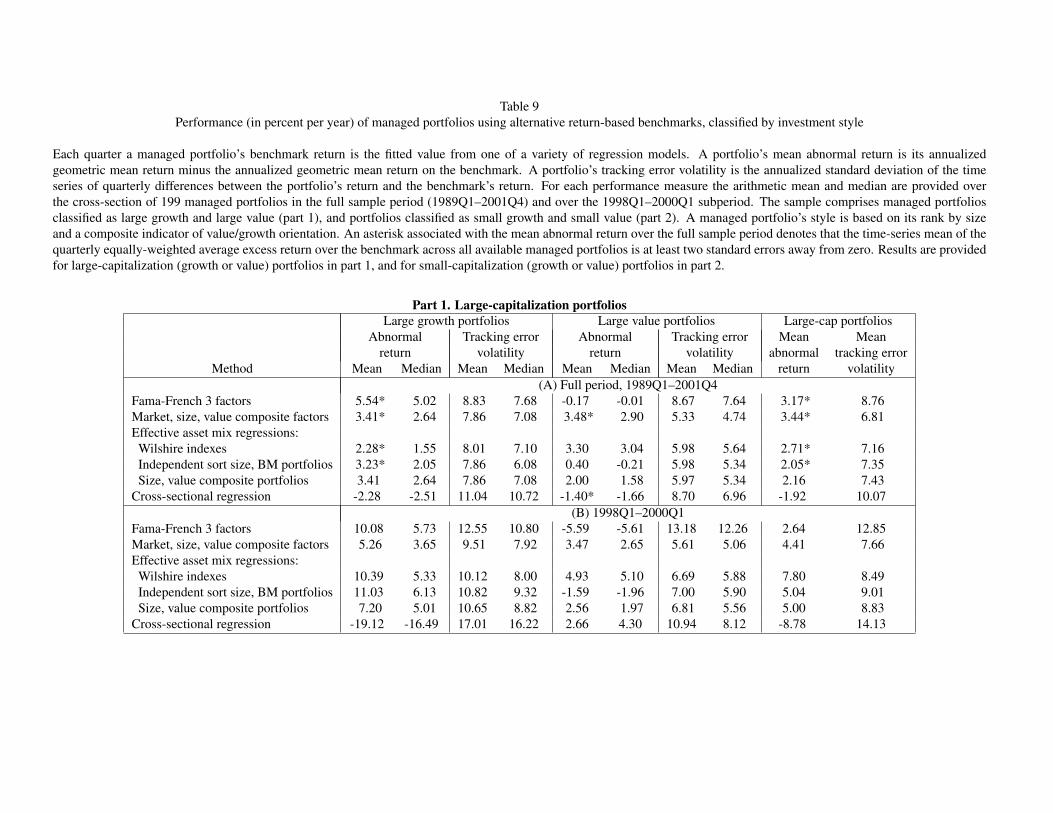
2.3 Results by investment style

Table 3 provides results across the entire set of managed portfolios. It is thus possible that systematic bench-

marking errors may not show up because they average out across the different styles followed by managers.

To see whether this is the case, Table 4 disaggregates the results on the benchmarking procedures by subsets

of managers who follow the same style. For the sake of brevity we only present results for the four key

styles: large value and growth, and small value and growth portfolios. Results are provided as well for the

aggregated set of large value and growth portfolios (denoted large-cap) and aggregated small-cap portfolios.

The results from Table 4 generally buttress the overall conclusions from Table 3. Even when we nar-

row attention to managers who follow the same style, there are striking differences across methods in mean

abnormal returns. To take the category of large growth portfolios as an example (part 1), average levels of ab-

normal return run the gamut from a paltry 0.24 percent relative to equal-weighted reference portfolios based

on size and the composite value indicator, to a dazzling 4.03 percent based on equal-weighted benchmarks

from independent sorts on size and book-to-market. For the combined sample of large growth and large value

portfolios the range in abnormal returns across methods is 2.20 percent, while for the combined sample of

small-stock portfolios in part 2 the range climbs to 4.60 percent.

Even larger differences in mean abnormal return estimates come to the fore during the overheated 1998–

2000 market. Benchmarks from independent sorts produce abnormal returns that, in absolute terms, generally

occupy the upper end of the range. Under this method, for example, large growth managers earn abnormal

returns of 10.85 percent relative to equal-weighted portfolios and 7.09 percent relative to value-weighted

benchmarks. The true level of manager skill in the sample is unknown, but average abnormal returns of this

magnitude challenge plausibility. When the reference portfolios are formed using a dependent sort by size

20

and then by the composite value indicator mean abnormal returns are lower. In the case of large growth man-

agers, mean abnormal returns from this method are 2.67 percent (1.52 percent) for equal-weighted (value-

weighted) benchmarks.

On the other hand large value managers severely underperform reference portfolios from independent

sorts. Their mean abnormal return averages -3.35 percent under equal-weighted benchmarks and -6.82 per-

cent under value-weighted benchmarks. The especially poor performance of large value managers under this

evaluation procedure underscores the pitfalls of treating size and book-to-market independently in forming

control groups. In particular, the procedure tends to pair large value managers with large growth benchmarks.

Since this reference group’s return is a high hurdle to overcome during the market boom of the late 1990s,

large value managers fare badly when compared to such an unrepresentative benchmark. (The following

section elaborates on the extent of the resulting mismatch.) Adopting the size-conditional, composite value

indicator paints a more accurate picture of a portfolio’s value-growth style, yielding estimates of abnormal re-

turns that are much less extreme. Mean abnormal returns are 0.15 percent under equal-weighted benchmarks

and -0.73 percent under value-weighted benchmarks.

Since the idiosyncratic component of returns is generally lower for large stocks, cross-method compar-

isons of tracking error volatilities are likely to be more informative when applied to the large stock port-

folios. Further, the bulk of institutional assets is concentrated in large-capitalization stocks. Accordingly

our discussion of the tracking error results in Table 4 focuses on the large growth and value managers.13

Control portfolios based on independent sorts and book-to-market ratios are generally associated with the

highest tracking error volatilities. For example, when large growth (large value) managers are confronted

with equally-weighted control portfolios from independent sorts the standard deviation of abnormal returns

is 9.64 percent (7.43 percent) on average. Moving to within-size sorts and a more comprehensive measure

to profile value/growth reduces mean tracking error volatility to 7.78 percent and 5.64 percent for the large

growth and large value subsets, respectively. In the combined large-stock manager sample the improvement

in tracking volatility is from 8.72 percent for equal-weighted independently sorted benchmarks to 6.89 per-

13The time clustering-adjusted F-statistic to test whether the equal-weighted portfolio of large-capitalization managers has equal

tracking error volatilities across methods is 2.23 with p-value of 0.04.

21

cent for equal-weighted benchmarks from sorts by size and the composite value indicator. The corresponding

reduction for value-weighted benchmarks is from 7.98 percent to 6.96 percent.

In the case of small stock portfolios (part 2), idiosyncratic return volatility is higher and smudges the dif-

ferences across methods in tracking error volatilities. Nevertheless, it is still the case that the independent sort

procedure performs poorly with respect to tracking ability compared to the size, composite value approach.

Under the latter approach, the average tracking error volatility for the combined set of small-capitalization

managers is 12.13 percent based on equal-weighting and 11.97 percent based on value-weighting.

For both large- and small-stock portfolios the tracking error volatilities convey the message that proce-

dures based on book-to-market as the sole measure of value-growth orientation perform poorly. Evidently,

book-to-market misses important information about return comovement. Treating as identical two similarly-

sized firms that have the same book value turns a blind eye to differences along other important dimensions

such as profitability, for instance.

3 Interpreting the evidence from characteristic-matching methods

The bottom line from the previous section is that the verdict on money manager performance is sensitive

to the choice of benchmarking method. This is the case even when we limit attention to apparently similar

procedures that build upon the same methodology of characteristic-matched portfolios. In this section we

trace the sources of the differences, with the objective of identifying the relative merits of each method. We do

this in several ways. First we apply the benchmarking procedures to a set of passive portfolios. This lets us see

how the methods fare in a controlled setting where there is no managerial skill, and the idiosyncratic return

component is low. These conditions help to bring the benchmarking methods’ performance into sharper

focus. Second we provide further details on the characteristics of the baseline portfolios from different

methods.

22

3.1 Results for passive indexes

Table 5 provides results when we take as our pseudo-active portfolios eight Russell style indexes: the Russell

top 200 growth and value indexes; the Russell midcap growth and value indexes; the Russell 1000 growth

and value indexes; and the Russell 2000 growth and value indexes. These indexes are the most commonly

used in the investment industry for evaluating managers.14 Table 5 also reports the simple average over the

eight indexes of: the abnormal return; the absolute abnormal return so positive and negative excess returns

do not cancel out; and the tracking error volatility.

The Russell indexes represent large, well-diversified portfolios which are, when compared to the man-

agers in our sample, less concentrated with a more stable composition. Accordingly, abnormal returns on the

indexes should not differ markedly from zero and the benchmarks should track the indexes closely. This po-

tentially affords more room for the different methods to stand out clearly from one another. Even with these

relatively well-behaved passive portfolios and long sample periods, however, the methods can yield quite

different conclusions with respect to estimated abnormal returns. In the case of the Russell 1000 growth

index, for example, the methods report net-of-benchmark returns that range from a low of -1.66 percent to a

high of 1.08 percent.

Taking the benchmarking methods to unmanaged indexes that are well-diversified with relatively fixed

make-up succeeds in spreading out tracking error volatility across methods. In particular the independent

sort procedure stands out for its poor covariation with the broad-based passive Russell indexes: in seven

out of the eight series this method yields the largest tracking error volatilities across methods. On the other

hand sorts by size and then by the composite value measure yield benchmarks that covary strongly with the

indexes. Averaged across all the indexes, this method produces tracking error volatilities of 3.41 percent

14Each of these indexes refers to growth or value stocks within a given size category. The largest 200 stocks by market capi-

talization constitute the top 200, while the next 800 make up the mid-capitalization group. The Russell 1000 comprises these two

groups. The Russell 2000 comprises the next largest 1000 stocks. Within each size category, stocks are ranked by a score based

on book-to-market ratio and analysts’ estimates of long-term earnings growth rates. Stocks are then assigned to value or growth

partitions such that half of the total market capitalization of the size category is in each partition. The return on the index is the

value-weighted average of the component stocks’ returns, where the weights are adjusted for cross-ownership and privately held

shares.

23

for equal-weighted reference portfolios, compared to 5.64 percent for baseline portfolios from independent

sorts. Restated in terms of the number of years necessary to declare a hypothetical mean abnormal return of

4 percent to be statistically significant at the ten percent level, the independent sort procedure would require

5.35 years while the size, composite value approach requires only 1.95 years.

The eye-catching differences across the methods during the 1998Q1–2000Q1 subperiod (part B of Table

5) highlight the shortcoming of book-to-market as a summary measure of value-growth style. Baseline port-

folios that measure value-growth orientation solely by book-to-market frequently give rise to large abnormal

returns. For example the abnormal return is 5.31 percent for the Russell 1000 growth index, and -5.64 percent

for the Russell 1000 value index, under the value-weighted, independent sort procedure. Estimated perfor-

mance levels of this magnitude for passive indexes strain credulity. Abnormal returns are generally closer

to zero when judged against reference portfolios that take other criteria into consideration when classifying

stocks as value or growth. With the capitalization-weighted size-conditional value composite method, the

abnormal return is 1.54 percent for the Russell 1000 growth index and 0.48 percent for the Russell 1000

value index.

3.2 Features of characteristic-matched portfolios

We concentrate on the features of reference portfolios from independent sorts on size and book-to-market.

This set of benchmarks is extensively used in the research literature, in no small part because the data are

easily accessible from Ken French’s website.

Table 6 reports the percentage of market capitalization accounted for by each of the twenty-five control

portfolios from independent sorts. The distribution is calculated at the beginning of each quarter from the

first quarter of 1989 to the last quarter of 2001. The results are averaged over quarters, and are provided for

four sub-periods: 1989Q1–1994Q4, 1995Q1–1997Q4, 1998Q1–2000Q1, and 2000Q2–2001Q4.

Not surprisingly, the top quintile of stocks accounts for the bulk of market capitalization. The discom-

fiting feature of the independent sort procedure, however, is the highly uneven split between growth and

value stocks within the large capitalization subset. In the first subperiod (panel A), the large growth category

represents 25.57 percent of the total value of listed domestic U.S. stocks while the large value group makes

24

up only 4.76 percent. As a result of the steep run-up in the prices of large growth firms during the market

boom, the relative importance of this group climbs in the late 1990s. Large growth stocks’ weight averages

46.36 percent in the 1998Q1–2000Q1 subperiod, and rises as high as 61.52 percent in the last subperiod

(2000Q2–2001Q4). Conversely, large value stocks shrink in importance from 3.39 to only 1.70 percent of

capitalization over the same subperiods.15

To rephrase the argument, the percentage amount in the cells of Table 6 can be interpreted as the dis-

tribution of assets across investors of different styles. From this perspective the independent sort procedure

suggests that in the late 1990s large-capitalization growth investors command as much as 14 times the assets

of large-capitalization value managers. In fact, the distribution of clients’ mandates is more evenly divided

between value and growth. Simply put, investors’ behavior does not conform to the classification produced

by independent sorts on size and book-to-market.

Part II of Table 6 provides the corresponding distribution of market capitalization for the classification

based on size and conditional book-to-market breakpoints. In comparison to the first part of the table, the

split of large stocks into growth and value partitions is more balanced. The large-growth category is much

less dominant, and its relative importance is more stable across sub-periods. Large growth stocks contribute

22.50 percent of market capitalization in the last subperiod, for example, compared to 15.97 percent in the

first subperiod.

Given the lopsided distribution produced by independent size and book-to-market breakpoints, the result-

ing benchmarks are heterogeneous portfolios that may be poorly aligned with more focused, active portfolios.

Table 7 documents the extent of the problem. Following up on the comparisons of the previous table, we

single out the large growth benchmark portfolios from either independent sorts, or from the size and con-

ditional book-to-market classification. Various attributes of each portfolio are reported in Table 7 to assess

where it falls along the value-growth spectrum. To ease comparison we express each attribute as equi-distant

percentile ranks from zero to one, so a stock with the highest value of the attribute (the most value-oriented

stock) receives a rank value of one while the stock with the lowest value of the attribute (the most growth-

15Since the composition of the categories is determined once a year (at the end of June), there is limited turnover in the make-up

of the groups. Accordingly some of the effects of the 1998–2000 market boom persist in the last sub-period.

25

oriented stock) receives a rank value of zero. Percentiles of the distribution of attribute ranks are calculated

over stocks in the portfolio and are then averaged over all quarters (panel A), or over the 1998Q1–2000Q1

subperiod (panel B).

In many studies a stock is considered as value or growth based on its book-to-market ratio, so this is the

first characteristic we consider. As other indicators of a stock’s value/growth profile, we also consider: cash

flow yield, dividend yield, earnings yield, and sales-to-price ratio.

Every measure of value-growth orientation exhibits large variation within the large-growth benchmark

from independent sorts (panel A). The earnings yield ranks of stocks in this group extend from 0.1062 at

the tenth percentile to 0.5242 at the ninetieth percentile. In comparison the large-growth benchmark based

on within-size breakpoints for book-to-market comprises a more homogeneous collection of stocks. Their

corresponding earnings yield ranks run from 0.1081 to 0.3832.16

Further, the large growth reference portfolio from independent classifications embraces many stocks that

would not generally be considered very growth-oriented. Based on the overall value indicator, for instance,

the 75th percentile of the distribution is 0.3978. Therefore, a quarter of the stocks in the portfolio score

above the fourth decile in terms of value-growth tilt within their size partition. In short, the large growth

benchmark from an independent size, book-to-market classification does not faithfully mirror the equity

class it purports to depict. Stated differently many of the stocks that a large value manager would hold in

practice are classified as large growth stocks under an independent sort procedure. The result of this scheme

is to pair off a large-capitalization value-oriented active manager with an unrepresentative reference portfolio.

The heterogeneity is exacerbated during the late 1990s (panel B). Within the large growth benchmark

from independent classifications, the spread between the 90th and 10th percentiles of the distribution of the

composite value indicator is 0.5815. A quarter of the stocks in the portfolio have a value indicator rank

in excess of 0.4769. On the other hand the size and conditional book-to-market classification produces a

benchmark portfolio that is more tightly focused in terms of its large growth orientation. The difference

16Note that the independent sort procedure uses New York Stock Exchange breakpoints for size and book-to-market. However,

our percentile ranks on book-to-market are determined relative to the cross-section of all listed domestic common stocks. As a result,

stocks classified as large growth under independent sorts do not necessarily have ranks that fall below 0.2.

26

between the 90th and 10th percentiles of the value composite score within this group is only 0.3058.

4 Regression-based benchmarks

Matching each stock in a managed portfolio against a control portfolio has the advantage of yielding poten-

tially more accurate measures of expected future returns. The disadvantage is that the data requirements are

more burdensome, since the portfolio manager’s holdings at the beginning of the period must be known. The

alternative is to work with the realized returns on the managed portfolio.

4.1 Three factor time-series regressions

Fama and French (1996) draw on the Merton intertemporal capital asset pricing model to develop a three

factor model of the form

rpt − rft = αp + βp(rmt − rft) + hpHMLt + spSMBt + εpt (1)

whererpt − rft is the return on portfoliop in montht in excess of the riskfree rate, andrmt − rft is the

excess return on the market.HMLt is the return on a zero investment factor-mimicking portfolio that is long

on value stocks and short growth stocks; similarly,SMBt the return on a zero investment factor-mimicking

portfolio that is long on small stocks and short large stocks. In the absence of stock selection ability,αp

should equal zero.

The bulk of the literature follows the lead of Fama and French (1996) in how the size and value/growth

factors are constructed. In particular, the size and value/growth factors are the differences between extreme

portfolios from independent sorts on size and book-to-market. To follow up on the evidence in the prior

sections suggesting that independent sorts tend to yield heterogeneous stock clusters, we develop alternative

mimicking portfolios. In particular, size is the difference between the value-weighted return on large stocks

(the 200 largest companies by equity market capitalization) and the value-weighted return on small stocks

(the thousand stocks ranked below 1000 when ordered by size). Similarly, because book-to-market equity

may be an incomplete description of a stock’s value/growth profile, we use our composite value measure

to define the value/growth factor. To construct our version of the value mimicking portfolio, we calculate

27

within each size cohort the difference in quarterly value-weighted returns between the top and bottom third

of stocks ranked by the composite. The spread is then averaged across size classes to yield the time series of

value factor returns.

Equation (1) accounts for the effects of size and value/growth separately, so the average benchmark

return on a portfolio adds a reward for smallness and a reward for value (in addition to the compensation

for market exposure). This may adequately describe return behavior over long periods, but it may not be

an innocuous assumption over the short horizons where performance is typically measured. Consider, for

example, a portfolio manager who concentrates in small value stocks, that is, who loads heavily on smallness

and on value. This investor will be held to a high predicted return when small stocks out-perform large

stocks. However the model posts a high expected return for smallness even if the only reason small stocks do

well is because small growth stocks out-perform. In this circumstance the hurdle is set too high for portfolios

of small value stocks and too low for small growth stock portfolios. Such an event occurs, for example,

in the first quarter of 2000, when small stocks (as measured by the Russell 2000 index) earned a return of

7.08 percent. This exceeds the return in the same quarter of 4.37 percent on the Russell 1000 index of large

stocks. In the small stock cohort, however, small growth stocks in the Russell 2000 growth index posted a

larger return (9.29 percent) than small value stocks in the Russell 2000 value index (3.82 percent).

4.2 Effective asset mix regressions

The three-factor regression model appears extensively in academic research. In the investment industry

an alternative regression-based benchmarking approach, due to Sharpe (1992), is more popular. An active

manager is seen as choosing stocks from equity subsets that vary across the size spectrum, and across the

value/growth spectrum. The return on the manager’s portfolio can thus be allocated into components corre-

sponding to the return on each subset. Any differential return reflects the manager’s skill.

We apply the Sharpe effective asset mix approach by estimating constrained regressions of the form

rpt = γp0 +K∑

j=1

γpjIjt + υpt (2)

whereIjt are the returns at timet on the equity sub-classes. The coefficientsγpj , j = 1, ...,K, represent

the proportions of portfoliop that are invested in each of theK classes. Since the equity managers in our

28

sample are limited to long positions in stocks, we prevent estimating counterfactual coefficients by imposing

the constraints that eachγpj ≥ 0, j = 1, ...,K, and∑K

j=1 γpj = 1.

Part of the popularity of Sharpe’s approach stems from its ease of interpretation, since the coefficients

can be readily interpreted as portfolio weights. Importantly, equation (2) uses the information in the returns

to each distinct equity asset class. Consequently it does not share the three-factor model’s shortcoming when

value and growth stocks behave differently across size cohorts.17

We use six equity style classes in equation (2): large value and growth, mid-cap value and growth, as

well as small value and growth. The returns on these classes are measured as the performance of either: the

Wilshire Target Indexes; the value-weighted benchmark portfolios from independent sorts that are used to

construct the Fama-French (1993) time series factors; and value-weighted reference portfolios from two-way

within-group sorts by size (small, mid and large-cap) and then by the composite value measure (value and

growth).18

4.3 Cross-sectional regression based benchmarks

Empirical research on asset-pricing models fits regressions of returns on attributes such as beta, size and

book-to-market (see, for example, Chan, Hamao and Lakonishok (1991) and Fama and French (1992)). The

thrust of this logic is that the fitted return from such a model can serve as the benchmark for an active

17In the three-factor model the mimicking portfolios for size and value are linear combinations of the returns on the equity

subclasses, as is the market portfolio. Substituting these definitions into the factor model equation (1) yields a regression of managed

portfolio returns on all the underlying equity subclass returns, with restrictions on the coefficients. For example, the portfolio’s

coefficient on the return to the small-cap value subclass,SV , can be written as13sp + 1

2hp + βpωSV wheresp is managed portfolio

p’s loading on the size factor,hp is its loading on the value factor,βp is its market beta, andωSV is the capitalization weight of

the small-cap value subclass relative to the market. Since the effective asset mix model corresponds to the full regression it should

produce lower tracking error volatilities, at least in-sample, if the non-negativity and summation constraints on the weights in the

Sharpe style regression are not inconsistent with the data. Note that another restriction of the three-factor model is that the sum of

the coefficients over equity subsets equals the portfolio’s market beta.18The Target style indexes, produced by Wilshire Associates, are concentrated passive portfolios constituting stocks that clearly

conform to high growth or high value features within a size bracket. Multiple criteria are used for this determination and they do not

necessarily overlap across the value and growth categories.

29

portfolio, given the attributes of the stock held by the manager.

We formulate this argument as follows. Each quarter we estimate the following cross-sectional regres-

sion:

rit = λ0t +L∑

j=1

λjtXjt + νit. (3)

rit is the return of stocki over quartert while Xjt are stock attributes at the beginning of the quarter. Given

estimates of the coefficientsλjt, j = 0, ..., L and the attributes of a stock, we calculate its fitted return from

equation (3). The benchmark return for an active portfolio is then the weighted average of the fitted returns

of the stocks held by the manager using beginning-of-quarter investment weights.

Equation (3) is well-known and extensively applied in financial research. In addition, it is the backbone

of several performance evaluation and attribution systems that are widely used in the investment industry

(see, for example, Barra (1990)). The model can be interpreted as a linear factor model for returns, where

stock attributes are assumed to be accurate measures of exposures to the underlying factors. The measured

coefficientλjt is an estimate of the realization of factorj in quartert.

Daniel and Titman (1997) find that a simple linear or log-linear model does not fully capture the associa-

tion between returns, size and book-to-market. To give the cross-sectional regression a fair shot at capturing

the behavior of returns we employ a specification that is parsimonious and reasonably robust. We include

the key variables that have been found in the literature to be important determinants of the cross-section

of average stock returns. The attributes are: size, book-to-market, cash flow to firm value, dividend yield,

earnings yield, sales-to-price ratio, past six-month return and industry dummy variables. Additionally the

effect of firm size (market capitalization) is captured through a set of five indicator variables. Depending

on where a stock’s market capitalization falls in the size distribution of NYSE firms, one of these indicators

takes the value of one and the others are zero. The ranges are: the top five percent of size; from the 80th to

the 95th percentile; between the 50th and 80th percentiles; between the 25th and 50th percentiles; the last is

for firm size below the 25th percentile. These size cohorts are meant to partition stocks into subsets roughly

corresponding to the equity investment domains of interest to managers. To mitigate problems with extreme

values of the fundamental characteristics, we use percentile rank values of the accounting attributes (from

zero for the lowest to one for the highest). Prior six-month returns for a stock are measured over a period

30

ending one month before the return measurement month. The industry dummy variables are based on the

Fama-French (1997) classification.

Equation (3) is typically applied in contexts where the objective is to uncover the determinants of returns

over relatively long horizons. Using it to pin down the behavior of short-horizon returns such as a month

or a quarter, as is done in practice, may be more treacherous. As a specific issue the linear specification of

the model assumes that the impact of a variable such as earnings yield is uniform across its entire range of

values. This is a questionable assumption over short horizons.

4.4 Results

Results for performance relative to regression-based benchmarks are reported in Table 8 for all managers.

The return predicted for a portfolio in a given quarter is based on that quarter’s realizations of the regressors

along with the estimated loadings from either equations (1), (2) or (3). Fitting the regressions to the manager’s

entire history increases the precision of the estimated loadings. However this tends to overfit the data, and as

a result confounds manager skill with the portfolio’s exposures. To avoid the pitfalls from overfitting, when

we estimate the predicted return in a quarter we leave that quarter out when we run the regressions. Both sets

of results are reported in the tables.

As with the characteristic-based benchmarks in Table 3, there is a wide range in abnormal returns esti-

mated from the regression-based benchmarks. Average abnormal returns for the entire sample of managers

over the full period (panel A of table 8) vary from 3.67 percent to -1.97 percent, yielding a range of 5.64

percent.19 Even when we narrow attention to the time-series regressions using factor-mimicking portfolios

mean abnormal returns are 2.64 percent and 3.67 percent on an out-of-sample basis. Similarly, the effective

asset mix regressions produce out-of-sample mean abnormal returns between 1.48 percent and 3.09 percent.

These differences stand out all the more because they are generated from models that closely resemble one

another, are fitted over many quarters and are averaged over numerous portfolios.

19A test that the regression-based methods all produce the same mean abnormal return for the equal-weighted portfolio of man-

agers yields a F-statistic (with standard error corrected for clustering by calendar quarter) of 5.20 with a p-value of less than 1

percent.

31

During the relatively short 1998Q1–2000Q1 subperiod (panel B) the difference across methods’ benchmark-

adjusted returns is even more acute, with the range rising to 14.31 percent. Within the set of Sharpe style

regressions out-of-sample abnormal returns display a range of 5.20 percent.

The message from Table 8 is that abnormal return estimates are very sensitive to the choice of regressors.

This is the case although the regressors tend to be highly correlated. For instance, in the effective asset

mix regressions the average pairwise correlation is 0.97 between the return series on the large growth style

indexes, and 0.88 for the large value style indexes. The overall average pairwise correlation between the

corresponding regressors in the style regressions is 92 percent.

The regressors from the various models share similar time-series properties. Moreover, the active portfo-

lio returns are noisy and have limited histories. These considerations limit our ability to discriminate clearly

between the procedures in terms of tracking error volatility.20 Nonetheless two procedures stand apart from

the others in terms of their poor out-of-sample performance. The cross-sectional regression approach in-

cludes a variety of stock attributes. However it generates the largest tracking error volatility of all the models

for the full period (10.60 percent).21 The tracking error volatility from the Fama-French three-factor model is

10.54 percent, which is substantially higher than the results from other methods. The volatility rises to 14.77

percent during the late 1990s. Not all is lost for the factor model, however. Revised factor-mimicking port-

folios for size and the size-conditional composite value indicator knock the out-of-sample tracking volatility

down to 8.33 percent for the overall period and 9.08 percent for the 1998–2000Q1 epoch.

Volatilities of tracking errors from the regresssion-based benchmarking models in Table 8 are roughly

comparable in magnitude to those from the characteristic-based models in Table 3. Capitalization-weighted

control portfolios from the size-dependent sort on the composite value indicator generate mean tracking error

volatilities of 8.71 percent for the full period and 9.44 percent for the 1998–2000 subperiod. This is in line

with the better regression-based models: the factor model using mimicking portfolios based on size and the

20For example, the F-statistic is 1.25 (p-value of 0.30) for the hypothesis that the equal-weighted portfolio of managers has the

same out-of-sample tracking error volatility across the methods in Table 8.21Some additional experiments suggest that several other specifications of the cross-sectional model yield even higher tracking

error volatility. In particular when the size variable is measured as the logarithm of market capitalization the mean tracking error

volatility rises to 13.04 percent.

32

composite value score produces an out-of-sample mean tracking error volatility of 8.33 percent for the full

period (9.08 percent for the late 1990s subperiod). However net-of-benchmark returns from the regression

models tend to be larger in absolute terms. In the case of the factor model for instance the average level of

manager performance, 3.67 percent, stretches belief.

Table 9 compares the performance of the regression-based benchmarks within each of four investment

styles. To minimize clutter we report results only for benchmarks that leave out the evaluation quarter from

the estimation period. The results reinforce the key findings from the overall sample in the previous table.

First, there is a large range across methods in mean abnormal returns, even when we limit attention to

homogeneous sets of portfolios. Within the category of large value managers, for example, the range across

methods in average performance levels is 4.88 percent. During the 1998–2000 subperiod the range is even

more breath-taking (10.52 percent). The dispersion in abnormal returns across procedures, as well as the

generally large absolute magnitude of mean abnormal returns, does not inspire confidence in the regression-

based benchmarks. In contrast the characteristic-based benchmarks in Table 4 produce abnormal returns that

are closer to zero, even during the 1998–2000 epoch.

Secondly, the tracking error volatilities of the large-capitalization portfolios are closely bunched with

the exception of the Fama-French factor model and the cross-sectional regression. In the case of large value

portfolios, for example, the tracking volatilities from these two procedures exceed 8.50 percent, while volatil-

ities from the other methods are much lower (less than 6 percent). For the reasons noted earlier large stock

portfolio tracking errors should provide a sharper means to discriminate between the models.

Third, large portfolios’ tracking volatilities from the regression-based benchmarks and the characteristic-

based benchmarks are generally comparable. When the characteristic-based methods are applied to the

combined large growth and value sample, the size, composite value indicator approach is associated with the

lowest tracking error volatility (6.89 percent). In the same sample the best-performing benchmark from the

regression models has a mean tracking volatility of 6.81 percent. However the estimated abnormal returns are

much more different: 0.54 percent from the characteristic-based approach as opposed to 3.44 percent from

the factor regression model. During the late 1990s average performance in the combined large-capitalization

sample is 1.47 percent under the characteristic-based procedure and 4.41 percent from the regression. Insofar

33

as the out-sized levels of performance from the regression models are hard to reconcile with intuition, the

advantage seems to go to the characteristic-based methods.

Fourth the volatile behavior of small stock returns generally prevents clear-cut distinctions between the

methods. Nonetheless the Fama-French factor model still turns in the poorest showing with respect to track-

ing error volatility. In the combined set of small-capitalization growth and value portfolios, the mean tracking

volatility is 14.73 percent for the overall period and 20.34 percent for the late 1990s.22 In contrast, for the

same set of portfolios the revised factor model based on size and the composite value score features a mean

tracking volatility of 11.93 percent in the overall period and 12.78 percent in the later sub-period.

5 Interpreting the evidence from regression-based methods

To discriminate more sharply between the benchmarks derived from regression models, we apply them to the

Russell indexes. Table 10 reports the results.

Passive indexes should yield no indication of performance. Further, the regression models are estimated

over the full thirteen-year history, so there should be little margin for disagreement. It is thus startling,

then, that the regression-based benchmarks produce sizeable spreads in abnormal returns. In the case of the

Russell 1000 growth index the range across methods exceeds 3 percent and in the case of the Russell 1000

value index the range is above 2 percent. The ranges are substantially larger for the small-stock indexes. For

the Russell 2000 value index for instance one method reports an impressive mean net-of-benchmark return of

3.36 percent, while another equally sensible method suggests that performance is a disastrous -3.36 percent.

The Fama-French factor model is at the core of academic research on investment performance. Tracking

error volatility from this approach, however, is exceptionally high. For instance out-of-sample tracking

volatility for the Russell 1000 growth index is 4.10 percent for the factor model. An adjustment to the factor

22While the cross-sectional regression method has poor tracking performance for large-stock portfolios, it performs on par with

the other methods for small-stock portfolios. The cross-section comprises many more small stocks than large, and the variation in

returns and attributes is more pronounced for small stocks than for large. As a result, the regression model tends to accommodate

the behavior of small stocks, everything else equal. Consequently fitted returns from the cross-sectional regression have an easier

time tracking small stocks.

34

model that uses a more comprehensive measure of value/growth within each size cohort is more successful.

Out-of-sample tracking error volatility is cut substantially to 2.38 percent. Averaged across all the indexes the

mean tracking volatility from the Fama-French three factor model is 4.99 percent, compared to 3.67 percent

using the modified size and composite value factors.23 The cross-sectional regression approach is popular in

academic research and widely used by practitioners as well. This method also shows subpar performance,

generating tracking volatilities of 5.42 percent for the Russell 1000 growth and 4.64 percent for the Russell

1000 value indexes.

Sharpe style regressions generally fare well. In asset mix regressions using the style portfolios underlying

SMB andHML out-of-sample standard deviations of abnormal returns average 4.07 percent. Regressions

that use the size, composite value reference portfolios produce mean tracking error volatilities of 3.49 percent.

The latter model generates the lowest tracking error volatility for six out of the eight indexes.24

The relatively well-behaved nature of the passive indexes provides leverage in discriminating between

the models’ performance. From this standpoint, the characteristic-based approach has a slight edge over the

regression-based approach. Of the characteristic-based models in Table 5 the best-performing benchmarking

model uses reference portfolios from sorts by size and then within each size group by the composite value

indicator. Tracking error volatilities from this approach average 3.01 percent. Characteristic matching pro-

cedures predict returns using stock attributes that are known at the beginning of the quarter. The most direct

23In additional experiments we verify that the bulk of the improvement stems from the modified value factor-mimicking portfolio

rather then the modified size factor. We do this by fitting a factor model that includes the market, the conventional size factorSML

used by Fama and French, and the value factor based on the composite value indicator. This approach yields a lower tracking error

volatility for six of the eight Russell indexes compared to a model that combines the market factor, the conventional Fama-French

value factorHML and the modified size factor.24The style regressions generally do poorly at tracking small-cap portfolios. One objection is that the regressors in the model

include large and mid-cap portfolios which are not relevant to a small-cap style. Since the regressors are correlated the regression

may try to allocate some weight to equity styles that the portfolio is not oriented toward, thus clouding tracking ability. When we

re-estimate the regressions using only small-cap style indexes as regressors the tracking error volatilities are reduced for the Russell

2000 growth index but not for the Russell 2000 value index. For example, in the Sharpe regression of the Russell 2000 growth

index on small-cap style portfolios from sorts on size and the composite value indicator the out-of-sample tracking volatility is 1.74

percent. Applied to the Russell 2000 value index the same model has a tracking volatility of 4.72 percent. Since we choose to apply

a uniform model to all portfolios, we do not pursue this modification of the Sharpe approach.

35

analogs are thus the regression procedures where the estimation period is divorced from the evaluation pe-

riod. Among the approaches in Table 10 the model with the best out-of-sample performance is the effective

asset mix regression using the same reference portfolios. The resulting standard deviation of tracking errors

is higher at 3.49 percent.

6 Benchmark choice and portfolio performance

An investor, financial advisor or money manager is concerned with how an individual portfolio performs.

The research literature and industry practice offer up an array of benchmarks, and a logical case can be made

for each of them. The issue therefore is the frequency of agreement across benchmarks with respect to over-

or under-performance, as well as the magnitude of differences in estimated abnormal returns across methods.

In this section we compare the benchmarks from this perspective.

Table 11 reports results when the methods are compared with respect to average abnormal returns over

the portfolio’s entire history (panel A), or with respect to annual and quarterly abnormal returns (panels B

and C). In panel A a portfolio’s average abnormal return over its full history is calculated as the difference

between the geometric mean return on the portfolio and on the benchmark. This is done under each of our

benchmarking methods (there are 20 procedures in total). We calculate all pairwise differences in abnormal

returns across methods and count the frequency of differences that exceed a threshold level (2.5 percent or 5

percent per year) out of the total of 190 possible comparisons. The relative frequency is then averaged across

portfolios. In addition we calculate the fraction of portfolios where the methods agree on the sign of the

abnormal return (all 20 are positive or they are all negative). Panels B and C perform the same calculations

using the time series of abnormal returns measured over each calendar year or each quarter, and averages the

results across portfolios and across time.

Since our benchmarking procedures share the premise that size and value/growth orientation are the

key drivers of average returns, the hope is that they should generally agree on the sign of a portfolio’s

performance, if not the magnitude of the performance. The results in Table 11 suggest that such consensus

happens less frequently than might be hoped. For all portfolios in the overall sample period the methods agree

on the sign of abnormal returns in only 20.60 percent of the cases (or in 79.40 percent of the cases there is

36

at least one disagreement about the sign of a portfolio’s abnormal return). The frequency of agreement for

individual styles varies from 25 percent for large value managers to as low as 13 percent for large growth

managers.

More specifically, the methods are likely to produce mean abnormal returns that deviate notably from one

another. For the entire sample absolute differences in excess of 2.5 percent per year occur with a frequency

of 39.79 percent, and absolute differences above 5 percent per year occur in 16.76 percent of the cases.

The chances of divergences in excess of the specified thresholds is generally higher for the small-stock

portfolios. As in the other tables, the likelihood of a large difference across methods rises during the 1998–

2000 subperiod. In the case of large value managers, for instance, the incidence of an absolute difference

above 5 percent jumps to 46.84 percent compared to 10.38 percent for the overall period.

Given the emphasis on performance, a few quarters of poor results can sour relations between a money

manager and clients. Panel B of Table 11 looks at the chances of disagreement as well as the magnitude of

differences across procedures in terms of year-by-year abnormal returns. Given the higher volatility of annual

observations rather than full-history averages, the divergences across procedures are starker in panel B. In an

average year the methods agree on the direction of performance with a frequency of only 18.56 percent, and

the chances of encountering absolute differences of above 5 percent in abnormal returns is 40.28 percent.

These results suggest that the choice of benchmarking procedure can make or break a money manager’s

reputation.

The evidence from yearly abnormal returns in panel B throws up a red flag about snap judgments re-

garding performance over short horizons. In practice, however, even a year is considered to be a long time

and manager performance is often scrutinized over shorter intervals. Panel C examines the frequency and

magnitudes of disagreements across methods with respect to quarterly abnormal returns. Note that the quar-

terly abnormal returns are roughly half as volatile as the annual series. Nevertheless the differences across

benchmarks yield a wide range of verdicts on performance. For all portfolios divergences in excess of one

percent per quarter occur with a frequency of 61.35 percent over the full sample period, with the incidence

growing to 69.13 percent in the 1998–2000 subperiod. Comparing the results from panels A to C in Table 11

offers the clear lesson that viewpoints about short-term performance rest on slippery footing. Averages over

37

longer horizons, while still prone to a wide range in benchmark estimates, may yield a clearer assessment of

individual manager performance.

7 Summary and conclusions

Professional money managers invest large amounts of equity assets on behalf of pension plan sponsors,

foundations, and individuals. In turn, clients are quick to hire and fire money managers on the basis of

benchmarking metrics that aim to identify precisely which managers have beaten and are expected to beat

the yardsticks. A large body of academic and practitioner research has extended the traditional capital as-

set pricing model and developed a broad array of methods to provide such benchmarks. Many of these

methods, at first glance, appear to be slight tweaks of a common methodological approach based on size

and value/growth as the main factors in the cross-section of returns. On the surface, then, it seems that the

methods should all deliver more or less the same assessment about the level of manager performance.

Our analysis of a detailed dataset on money manager performance suggests that this is not the case. We

use several variants of matched-characteristic reference portfolios and time-series return regressions to check

for performance. Estimated abnormal returns display large variation across procedures. For the sample

of investment managers following a large growth style, for instance, the range in mean abnormal returns

across characteristic-based benchmarking methods is 3.79 percent and 7.82 percent across regression-based

methods. The corresponding range across methods for large value managers is 1.73 percent and 4.88 percent.

Divergences across the methods in measured levels of performance are dramatically amplified during the

overheated market conditions of 1998Q1–2000Q1. For the characteristic-based methods the spread in mean

abnormal returns of large growth portfolios is 9.33 percent and across the regression-based methods it is 30.15

percent. Applied to large value portfolios characteristic-based methods produce a range of 6.97 percent and

regression-based methods generate spreads of 10.52 percent. These stark differences arise even though all

the methods draw on the same premise that size and value/growth are the key drivers of stocks’ average

returns. As well, the methods are applied over a relatively extended period and averaged across numerous

active portfolios.

Put another way different methods applied to the same portfolio manager can produce abnormal returns

38

that disagree dramatically with respect to sign and magnitude. In practice managers are hired and fired on

the basis of performance over short horizons. In an average year our full set of benchmarking methods agree

on the sign of abnormal return with a frequency of only 18.56 percent. When the methods are compared in

terms of the level of estimated abnormal returns in an average year, differences across methods in excess of

5 percent per year occur in 40.28 percent of the portfolios.

The import of these findings is that they suggest the following scenario can frequently occur. Suppose a

client specifies a benchmark for an asset manager that correctly corresponds to the manager’s style. Relative

to this yardstick the manager could out-perform, perhaps even by a statistically significant margin. The

client, however, could have selected another benchmark that is just as legitimate for the manager’s style. Our

results suggest that it need not be surprising to find that the same manager, without any change in behavior,

underperforms the alternative yardstick. The frailty of inferences to the choice of benchmarking procedure, if

not recognized, can impose substantial real costs. The process of terminating a manager whose performance

is deemed to be unsatisfactory consumes resources. These expenses come in the form of hiring a transition

manager, liquidating the portfolio and the costs of searching for a replacement.

Our results let us assess the performance of benchmarking methods that have been extensively used

in academic research and investment practice. Of these, the leading procedures that are widely used in

academic research — characteristic-matched portfolios based on independent sorts by size and book-to-

market, the three-factor time series model with mimicking portfolios for size and book-to-market, and cross-

sectional regressions of returns on a variety of predictors — have disappointing performance. They have poor

ability to track the returns of both active and passive portfolios. As well, they are frequently associated with

implausible levels of over- or under-performance. Reference portfolios from independent sorts by size and

book-to-market produce average abnormal returns of 5.31 percent when applied to the passive Russell 1000

growth index during the 1998Q1–2000Q1 period, and indicate performance of -5.64 percent for the Russell

1000 value index over the same period. For the same unmanaged indexes the cross-sectional regression

approach reports performance levels of -8.15 percent and 8.11 percent. We trace the poor showing of these

methods to underlying drawbacks in the design of the benchmarks.

Importantly, we discuss simple alterations that improve the performance of the benchmarking methods.

39

Two-way within group sorts by size and value/growth reflect more accurately the investment domains of

equity asset managers. A comprehensive measure that takes other variables beyond book-to-market equity

into account also matches portfolios’ value/growth orientations better. More generally, benchmarks that are

aimed at capturing the characteristics of active portfolios generally tend to have better performance than

regression-based benchmarks. Capitalization-weighted control portfolios that match a managed portfolio’s

size and composite value indicator, when applied to the sample of active managers over the full period,

produce a mean abnormal return of 0.78 percent and an average tracking error volatility of 8.71 percent. In

comparison the most widely applied benchmarking method in the academic research literature, the Fama-

French three factor regression model, generates a mean abnormal return of 2.64 percent and tracking error

volatility of 10.54 percent. In the case of passive Russell indexes, the characteristic-matched procedure has

an average tracking error volatility of 3.01 percent, compared to 4.99 percent for the three-factor model.

Our results are derived from a broad sample of managers, representing a variety of styles, and covering an

extended period. Even so, the findings underscore the fuzziness surrounding judgments on investment per-

formance, even in a standard context which is supposedly well-understood. As such, verdicts on performance

based on short horizons and overfitted models should be regarded with a healthy dose of skepticism.

40

References

Barber, Brad M., and John D. Lyon, 1997, Detecting long-run abnormal stock returns: The empirical power

and specification of test statistics,Journal of Financial Economics43, 341–372.

BARRA, 1990,The United States Equity Handbook, BARRA, Berkeley.

Brancato, Carolyn Kay, and Stephan Rabimov, 2005, The 2005 institutional investment report: U.S. and

international trends, Conference Board.

Brav, Alon and Paul Gompers, 1997, Myth or reality? The long-run underperformance of initial public

offerings: Evidence from venture and non-venture capital-backed companies,Journal of Finance52,

1791–1821.

Carhart, Mark M., 1997, On persistence in mutual fund performance,Journal of Finance52, 57–82.

Chan, Louis K. C., Hsiu-Lang Chen, and Josef Lakonishok, 2002, On mutual fund investment styles,Review

of Financial Studies15, 1407–1437.

Chan, Louis K. C., Yasushi Hamao, and Josef Lakonishok, 1991, Fundamentals and stock returns in Japan,

Journal of Finance46, 1749–1764.

Chan, Louis K. C., Jason Karceski, and Josef Lakonishok, 1999, On portfolio optimization: Forecasting

covariances and choosing the risk model,Review of Financial Studies12, 937–974.

Chan, Louis K. C., Jason Karceski, and Josef Lakonishok, 2000, New paradigm or same old hype in equity

investing?,Financial Analysts Journal56, 23–36.

Chan, Louis K. C., Josef Lakonishok, and Theodore Sougiannis, 2001, The stock market valuation of research

& development expenditures,Journal of Finance56, 2431–2456.

Coggin, T. Daniel, Frank J. Fabozzi, and Shafiqir Rahman, 1993, The investment performance of U.S. equity

pension fund managers: An empirical investigation,Journal of Finance48, 1039–1055.

Daniel, Kent, and Sheridan Titman, 1997, Evidence on the characteristics of cross sectional variation in stock

returns,Journal of Finance52, 1–33.

41

Daniel, Kent, Mark Grinblatt, Sheridan Titman, and Russ Wermers, 1997, Measuring mutual fund perfor-

mance with characteristic-based benchmarks,Journal of Finance52, 1035–1058.

Elton, Edwin J., Martin J. Gruber, Sanjiv Das, and Matthew Hlavka, 1993, Efficiency with costly information:

A reinterpretation of evidence for managed portfolios,Review of Financial Studies, 1–22.

Fama, Eugene F., 1998, Market efficiency, long-term returns and behavioral finance,Journal of Financial

Economics49, 283–306.

Fama, Eugene F., and Kenneth R. French, 1992, The cross-section of expected stock returns,Journal of

Finance46, 427–466.

Fama, Eugene F., and Kenneth R. French, 1993, Common risk factors in the returns on bonds and stocks,

Journal of Financial Economics33, 3–56.

Fama, Eugene F., and Kenneth R. French, 1996, Multifactor explanations of asset pricing anomalies,Journal

of Finance51, 55–87.

Fama, Eugene F., and Kenneth R. French, 1997, Industry costs of equity,Journal of Financial Economics43,

153–193.

Gruber, Martin J., 1996, Another puzzle: The growth in actively managed mutual funds,Journal of Finance

51, 783–810.

Ikenberry, David, Josef Lakonishok, and Theo Vermaelen, 1995, Market underreaction to open market share

repurchases,Journal of Financial Economics39, 181–208.

Jensen, Michael C., 1968, The performance of mutual funds in the period 1945–64,Journal of Finance23,

389–416.

Kothari, S. P., and Jerold B. Warner, 2001, Evaluating mutual fund performance,Journal of Finance56,

1985–2010.

Lakonishok, Josef, and Inmoo Lee, 2001, Are insider trades informative?,Review of Financial Studies14,

79–111.

42

Lakonishok, Josef, Andrei Shleifer, and Robert W. Vishny, 1992, The structure and performance of the money

management industry,Brookings Papers on Economic Activity: Microeconomics, 339–391.

Lakonishok, Josef, Andrei Shleifer, and Robert W. Vishny, 1994, Contrarian investment, extrapolation, and

risk, Journal of Finance49, 1541–1578.

Lyon, John D., Brad M. Barber, and Chih-Ling Tsai, 1999, Improved methods for tests of long-run abnormal

stock returns,Journal of Finance54, 165–201.

Malkiel, Burton G., 1995, Returns from investing in equity mutual funds, 1971–1991Journal of Finance50,

549–572.

Mitchell, Mark L., and Erik Stafford, 2000, Managerial decisions and long-term stock price performance,

Journal of Business73, 287–329.

43

Table 1Frequency of differences in measured abnormal return across benchmarksbased on characteristic-matched control portfolios and three-factor model

A managed portfolio’s performance is measured relative to one of two benchmarking methods. In the firstmethod the benchmark is based on control portfolios that match the size and book-to-market characteris-tics of each stock held in the portfolio. In the second method the benchmark return is based on a 3-factortime-series model regression. In panel A, benchmarks are assessed based on the active portfolio’s averageabnormal return (the difference between the portfolio’s geometric mean return and the benchmark’s geomet-ric mean return). The results tabulate the number of portfolios (out of a total of 199 active managers in thesample) where the two methods yield mean abnormal return estimates that differ in sign, as well as the frac-tion where the absolute difference in estimated abnormal annualized return exceeds either 2.5 or 5 percentper year. In panels B and C, abnormal returns (portfolio return minus benchmark return) are measured foreach full calendar year over a portfolio’s history or each quarter, respectively, from each method. For eachportfolio, the fraction of years or quarters where the two methods disagree on the sign of the abnormal returnis calculated, as well as the fraction where the absolute difference between the abnormal returns exceeds athreshold level. The fractions are then averaged across all portfolios in the sample. The threshold levelsare 2.5 and 5 percent per year, or 1 and 3 percent per quarter. Results are provided for all active portfoliosand portfolios classified by investment style, over the full period 1989Q1–2001Q4 as well as during the1998Q1–2000Q1 subperiod.

Panel A. Average abnormal annualized returnPercentage of comparisons yielding:

Different Absolute differences above: Different Absolute differences above:Sample signs 2.5% 5% signs 2.5% 5%

(A) Full period, 1989Q1–2001Q4 (B) 1998Q1–2000Q1 subperiodAll portfolios 0.2462 0.4322 0.1407 0.1750 0.6438 0.4375Large growth 0.1111 0.3111 0.0889 0.1936 0.7742 0.6129Large value 0.2188 0.4688 0.0313 0.0714 0.4643 0.2143Small growth 0.5000 0.6429 0.4286 0.1111 1.0000 0.7778Small value 0.1429 0.3571 0.0000 0.0769 0.7692 0.5385

Panel B. Annual abnormal returnPercentage of comparisons yielding:

Different Absolute differences above: Different Absolute differences above:Sample signs 2.5% 5% signs 2.5% 5%

(A) Full period, 1989Q1–2001Q4 (B) 1998Q1–2000Q1 subperiodAll portfolios 0.2449 0.6565 0.4136 0.3453 0.7818 0.6235Large growth 0.2156 0.5248 0.2886 0.2533 0.7067 0.5867Large value 0.3016 0.7214 0.4245 0.4861 0.8750 0.7361Small growth 0.2540 0.8077 0.5664 0.2963 0.9259 0.7778Small value 0.2324 0.7466 0.5436 0.2564 0.8205 0.6410

Panel C. Quarterly abnormal returnPercentage of comparisons yielding:

Different Absolute differences above: Different Absolute differences above:Sample signs 1% 3% signs 1% 3%

(A) Full period, 1989Q1–2001Q4 (B) 1998Q1–2000Q1 subperiodAll portfolios 0.2898 0.6953 0.3502 0.3285 0.8389 0.5153Large growth 0.2702 0.6185 0.2518 0.3118 0.8065 0.4444Large value 0.3084 0.6697 0.3140 0.4008 0.8333 0.5714Small growth 0.2832 0.8461 0.6310 0.3704 0.9383 0.8395Small value 0.3357 0.7671 0.4417 0.3419 0.7521 0.4530

For the characteristic-matched benchmarking procedure, each stock in the active portfolio at the beginning of aquarter is matched against a control portfolio based on beginning-quarter values of size (market capitalization of eq-uity) and book-to-market value of common equity. There are 25 control portfolios from the intersection of independentsorts by size and the ratio of book value of common equity to the market value of common equity. The control port-folio’s return is the equally-weighted average of the buy-and-hold quarterly returns on the component stocks. Controlportfolios are reformed at the beginning of July each year. In the 3-factor model, the benchmark return is the fittedvalue from a regression of quarterly active portfolio returns on the market excess return and returns on mimickingportfolios for size and book-to-market, SMB and HML. The regression uses all quarters over the sample period toestimate coefficients.

Table 2Relationship between portfolio abnormal return, net growth in portfolio assets

and growth in number of accounts

The sample comprises 340 institutional U.S. equity portfolios over the period 2000-2004. A managed portfolio’sabnormal return is the difference between its geometric mean annual return from 2000–2004 and the geometric meanannual return over the same period on the Russell benchmark corresponding to its investment style. The styles are:large growth, large value, small growth and small value. Within each style, portfolios are ranked by abnormal returnand placed in one of four quartile groups. The median net growth of portfolio assets (growth in portfolio assets undermanagement less the cumulative return on the beginning assets) and median growth rate of the number of accounts inthe portfolio from 2001–2004 are calculated for each quartile group. The flow-return sensitivity is the slope coefficientfrom a regression of the net growth in portfolio assets or growth in the number of accounts on portfolio abnormalannualized return (in percent).

Quartile by return in excessof Russell benchmark: Flow-return

Sample Statistic 1 2 3 4 sensitivityAll Mean excess return (%) -3.35 1.27 4.61 10.17

Median asset growth -0.3284 0.1345 0.6519 1.6036 1.16Median account growth -0.2222 0.1402 0.6369 1.2000 0.19

Large growth Mean excess return (%) -1.27 3.23 5.95 10.58Median asset growth -0.1751 0.1505 1.3738 1.6566 0.31Median account growth -0.5000 0.0484 1.2284 0.9475 0.24

Large value Mean excess return (%) -2.94 0.09 2.57 7.76Median asset growth -0.2964 -0.1955 1.1592 1.2194 1.94Median account growth -0.1798 0.2000 0.6000 1.5685 0.33

Small-cap growth Mean excess return (%) -3.85 3.28 6.66 13.28Median asset growth -0.4391 0.1345 0.2352 1.2186 0.90Median account growth -0.6364 0.1429 0.2174 1.0000 0.14

Small-cap value Mean excess return (%) -4.41 -0.03 2.40 6.37Median asset growth -0.8004 0.2168 0.5454 7.9538 1.47Median account growth 0.0000 0.0636 1.0000 4.2500 0.06

Net growth in portfolio assets is calculated as:

(Aend −Abegin(1 + rp)4)Abegin

where Abegin, Aend are assets under management in the portfolio at the beginning of 2001 and at the end of 2004,respectively, and rp is the portfolio’s geometric mean annual rate of return from 2001 to 2004. Growth in the numberof accounts is measured as:

((nend

nbegin)− 1)

where nbegin,nend are the number of accounts investing in the portfolio at the beginning of 2001 and at the end of2004, respectively.

Table 3Performance (in percent per year) of managed portfolios using alternative holdings-based benchmarks

At the beginning of a quarter each stock held in a managed portfolio is matched against a control portfolio based on its characteristics, using one of severalprocedures. The subsequent quarter’s return on the managed portfolio, and the weighted average of the buy-and-hold returns on the controls are calculated;the procedure is repeated in the next quarter. Statistics are provided for each managed portfolio’s mean abnormal return and tracking error volatility overthe entire sample period (1989Q1–2001Q4), and during 1998Q1–2000Q1. A portfolio’s mean abnormal return is its annualized geometric mean returnminus the annualized geometric mean return on the benchmark. A portfolio’s tracking error volatility is the annualized standard deviation of the timeseries of quarterly differences between the portfolio’s return and the benchmark’s return. For each performance measure the arithmetic mean and medianare provided over the cross-section of managed portfolios in the sample period. The sample comprises 199 managed portfolios. The t-statistic for thehypothesis that the time-series mean of the quarterly equally-weighted average excess return over the benchmark across all available managed portfoliosequals zero is reported. Also reported are mean absolute differences between the characteristic ranks of the managed portfolios and benchmarks undereach procedure with respect to size, book-to-market and the composite value indicator.

Annual independent Annual size, Annual size, Quarterly size,size, BM within-size BM value composite within-size BM

Equal Value Equal Value Equal Value Equal Value Russellweight weight weight weight weight weight weight weight index

(A) Full period, 1989Q1–2001Q4Mean 2.06 1.39 1.33 1.13 0.79 0.78 0.72 0.71 2.72

Abnormal return Median 1.96 1.10 0.94 0.87 0.60 0.45 0.46 0.33 2.26Std Dev 4.26 4.27 4.50 4.63 4.41 4.47 4.57 4.64 4.50t-stat 1.38 3.57 1.52 3.02 1.33 1.46 1.72 2.23 4.90

Tracking error Mean 10.37 9.35 9.51 8.97 8.72 8.71 9.01 8.80 8.94volatility Median 9.00 7.90 8.16 7.80 7.28 6.86 7.74 7.46 7.92Mean absolute Size 0.028 0.010 0.029 0.008 0.034 0.014 0.035 0.015 0.093difference of Book-to-market 0.031 0.031 0.012 0.010 0.029 0.029 0.012 0.010 0.067characteristic ranks Value composite 0.089 0.082 0.064 0.059 0.017 0.012 0.065 0.060 0.090

(B) 1998Q1–2000Q1Mean 3.37 0.65 3.14 0.70 2.12 1.67 0.75 0.84 2.21

Abnormal return Median 1.09 -2.31 1.06 -1.19 1.28 0.77 -1.53 -2.00 0.54Std Dev 14.08 14.13 13.55 13.20 10.85 11.21 13.64 13.94 12.59

Tracking error Mean 10.70 10.29 10.04 9.98 9.43 9.44 10.02 9.81 9.34volatility Median 8.80 8.28 7.82 7.90 7.32 7.30 7.86 8.08 7.52Mean absolute Size 0.027 0.011 0.029 0.008 0.034 0.013 0.036 0.015 0.090difference of Book-to-market 0.031 0.032 0.012 0.010 0.028 0.028 0.012 0.010 0.072characteristic ranks Value composite 0.092 0.087 0.066 0.062 0.017 0.012 0.068 0.063 0.089

The benchmarking procedures are as follows. Each stock held in a managed portfolio at the beginning of a quarter is matched against a controlportfolio. Under the independent sorting procedure, there are 25 control portfolios from the intersection of independent sorts by size (market value ofequity) and BM (the ratio of book value of common equity to the market value of common equity). Under the size, within-size BM sort procedure thereare 28 control portfolios from sorts first by size, and then within each size category, by BM. In the size, value composite approach a stock is given an

overall ranking, conditional on its size group, based on book-to-market, dividend yield, cash flow yield, average earnings yield (based on the past year’snet income, forecasted next year earnings, and forecasted two-year ahead earnings), and sales-to-price ratio. In these methods the component stocks in acontrol portfolio are refreshed once a year at the end of June. In the quarterly size, within-size BM approach the component stocks are refreshed at thebeginning of each quarter. The return on a control portfolio is either the equally-weighted or value-weighted average of the buy-and-hold returns on thecomponent stocks. Each managed portfolio is also paired with a Russell style index depending on its investment style based on size and conditional valuecomposite indicator.

Table 4Performance (in percent per year) of managed portfolios using alternative

holdings-based benchmarks, classified by investment style

At the beginning of a quarter each stock held in a managed portfolio is matched against a control portfolio based on its characteristics, using one of several procedures. Thesubsequent quarter’s return on the managed portfolio, and the weighted average of the buy-and-hold returns on the controls are calculated; the procedure is repeated in thenext quarter. Statistics are provided for the managed portfolios’ abnormal returns and tracking error volatilities over the entire sample period (1989Q1–2001Q4), and overthe 1998Q1–2000Q1 subperiod. A portfolio’s abnormal return is its annualized geometric mean return minus the annualized geometric mean return on the benchmark. Aportfolio’s tracking error volatility is the annualized standard deviation of the time series of quarterly differences between the portfolio’s return and the benchmark’s return.For each performance measure the arithmetic mean and median are provided over the cross-section of managed portfolios in the sample period. For results based on the fullsample period, an asterisk associated with the arithmetic mean abnormal return denotes that the time series mean of the quarterly equally-weighted average excess returnover the benchmark across all available managed portfolios is at least two standard errors away from zero. Results are provided for large-capitalization (growth or value)portfolios in part 1, and for small-capitalization (growth or value) portfolios in part 2.

Part 1: Large-capitalization portfoliosLarge growth portfolios Large value portfolios Large-cap portfolios

Abnormal Tracking error Abnormal Tracking error Mean Meanreturn volatility return volatility abnormal tracking error

Method Mean Median Mean Median Mean Median Mean Median return volatility(A) Full period, 1989Q1–2001Q4

Annual independent size, BMEqual weight 4.03* 3.84 9.64 8.40 0.60 0.43 7.43 6.48 2.60 8.72Value weight 2.11* 2.00 8.55 6.94 0.02 0.94 7.19 6.88 1.24* 7.98

Annual size, within-size BMEqual weight 2.97* 2.72 8.58 6.84 -0.25 -0.46 6.65 5.72 1.63* 7.78Value weight 2.32* 2.25 7.99 6.22 -0.35 -0.82 6.64 5.54 1.21* 7.42

Annual size, value compositeEqual weight 0.24 -0.23 7.78 7.00 0.96 0.91 5.64 4.84 0.54 6.89Value weight 0.28 0.33 7.91 6.56 0.56 0.48 5.62 4.80 0.40 6.96

Quarterly size, within-size BMEqual weight 1.60* 1.37 8.10 6.68 -0.60 -0.73 6.32 5.40 0.69* 7.36Value weight 1.47* 1.15 7.97 6.48 -0.64 -0.56 6.20 5.28 0.59* 7.24

Russell 3.28* 3.40 8.83 7.74 1.09 0.96 6.15 4.96 2.37* 7.72(B) 1998Q1–2000Q1

Annual independent size, BMEqual weight 10.85 8.54 11.67 9.48 -3.35 -3.93 7.72 5.86 4.11 9.79Value weight 7.09 3.99 10.76 7.78 -6.82 -7.09 8.01 6.90 0.49 9.45

Annual size, within-size BMEqual weight 10.69 7.01 10.88 8.60 -4.07 -4.58 6.79 5.64 3.68 8.94Value weight 6.41 3.02 9.77 7.52 -5.51 -6.34 7.58 6.10 0.75 8.73

Annual size, value compositeEqual weight 2.67 2.02 9.56 7.90 0.15 0.68 6.47 4.68 1.47 8.09Value weight 1.52 1.86 9.64 7.08 -0.73 0.30 6.58 4.64 0.45 8.19

Quarterly size, within-size BMEqual weight 4.97 3.07 10.24 9.26 -4.86 -4.92 6.86 5.30 0.31 8.64Value weight 4.78 2.30 10.01 8.46 -5.10 -4.83 6.83 5.28 0.09 8.50

Russell 3.12 0.70 9.93 8.40 -2.24 -1.69 6.48 5.44 0.58 8.30

Part 2: Small-capitalization portfoliosSmall growth portfolios Small value portfolios Small-cap portfolios

Abnormal Tracking error Abnormal Tracking error Mean Meanreturn volatility return volatility abnormal tracking error

Method Mean Median Mean Median Mean Median Mean Median return volatility(A) Full period, 1989Q1–2001Q4

Annual independent size, BMEqual weight 2.89 1.04 15.52 14.86 -0.90 -1.14 11.80 11.00 1.00 13.66Value weight 3.08 0.95 14.21 13.84 0.23 0.51 10.68 9.36 1.66 12.44

Annual size, within-size BMEqual weight 2.43 0.41 15.12 14.80 -1.52 -2.32 11.58 10.86 0.45 13.35Value weight 2.69* 0.84 13.93 13.74 -0.53 -1.09 10.49 9.46 1.08 12.21

Annual size, value compositeEqual weight -1.91 -3.47 14.32 13.98 2.36 2.41 9.93 7.82 0.23 12.13Value weight -1.48 -2.86 14.23 13.60 2.76* 2.44 9.70 7.25 0.64 11.97

Quarterly size, within-size BMEqual weight 3.43* 1.67 13.95 14.04 -2.11 -2.76 10.66 9.80 0.66 12.30Value weight 3.30* 1.47 13.72 13.08 -1.65 -2.52 10.19 9.04 0.82 11.96

Russell 7.28* 6.52 12.85 12.04 2.38* 2.13 7.73 6.84 4.83* 10.29(B) 1998Q1–2000Q1

Annual independent size, BMEqual weight 13.94 12.90 17.36 15.56 -8.35 -9.51 9.42 8.86 0.77 12.67Value weight 13.00 11.88 16.50 14.22 -7.78 -9.08 9.73 7.62 0.72 12.50

Annual size, within-size BMEqual weight 13.03 10.97 16.83 15.78 -8.11 -10.92 8.90 8.36 0.53 12.14Value weight 11.95 8.43 15.71 15.92 -8.42 -11.45 9.66 8.10 -0.09 12.14

Annual size, value compositeEqual weight -3.08 -4.81 13.07 11.76 -0.76 -2.19 8.68 7.00 -1.71 10.48Value weight -1.44 -3.23 13.02 12.00 0.24 -1.12 8.78 6.90 -0.45 10.51

Quarterly size, within-size BMEqual weight 12.46 10.28 16.20 15.74 -9.42 -12.08 9.20 8.58 -0.47 12.06Value weight 13.29 10.80 15.81 14.40 -8.04 -11.19 8.96 8.22 0.69 11.76

Russell 12.18 11.97 14.58 13.34 2.87 0.82 7.81 6.18 6.68 10.58

The benchmarking procedures are as follows. Each stock held in a managed portfolio at the beginning of a quarter is matched against a control portfolio. Under theannual independent size, BM procedure, there are 25 control portfolios from the intersection of independent sorts by size (market value of equity) and BM (the ratio ofbook value of common equity to the market value of common equity). Under the annual size, within-size BM procedure there are 28 control portfolios from sorts first bysize, and then within each size category, by BM. In the annual size, value composite approach a stock is given an overall ranking, conditional on its size group, based onbook-to-market, dividend yield, cash flow yield, average earnings yield (based on the past year’s net income, forecasted next year earnings, and forecasted two-year aheadearnings), and sales-to-price ratio. In these methods the component stocks in a control portfolio are refreshed once a year at the end of June. In the quarterly size, within-sizeBM approach the component stocks are refreshed at the beginning of each quarter. The return on a control portfolio is either the equally-weighted or value-weighted averageof the buy-and-hold returns on the component stocks. Each managed portfolio is also paired with a Russell style index depending on its investment style based on size andconditional value composite indicator.

Table 5Performance (in percent per year) of Russell style indexes using alternative holdings-based benchmarks

At the beginning of a quarter each stock in a Russell style index is matched against a control portfolio based on its characteristics, using one of severalprocedures. The subsequent quarter’s return on the index, and the weighted average of the buy-and-hold returns on the control portfolios are calculated; theprocedure is repeated in the next quarter. For each index statistics are provided for the abnormal return and tracking error volatility over the entire sampleperiod (1989Q1–2001Q4), and for the 1998Q1–2000Q1 subperiod. The abnormal return is the annualized geometric mean return on the index minus theannualized geometric mean return on the benchmark portfolio. An asterisk denotes that the mean abnormal return is more than two time-series standarderrors away from zero. The tracking error volatility is the annualized standard deviation of the time series of quarterly differences between the index returnand the benchmark’s return. The indexes are: the Russell top 200 (value and growth); the Russell midcap (value and growth); the Russell 1000 (value andgrowth); and the Russell 2000 (value and growth).

(A) Full period, 1989Q1–2001Q4Annual independent Annual size, Annual size, Quarterly size,

size, BM within-size BM value composite within-size BMEqual Value Equal Value Equal Value Equal Valueweight weight weight weight weight weight weight weight

Top 200 Growth Abnormal return 1.05 -0.18 0.48 0.33 -1.60 -1.12 0.20 0.46Tracking error 5.68 3.68 4.06 3.00 3.42 2.12 2.58 3.34

Top 200 Value Abnormal return 1.70 1.52 1.14 0.97 0.29 -0.17 0.69 0.61Tracking error 6.74 4.64 3.82 3.76 2.72 2.58 3.04 3.12

Midcap Growth Abnormal return 1.23 0.88 1.91 1.19 -1.79 -2.04 2.33 2.78*Tracking error 8.38 9.62 6.72 5.72 4.28 4.36 6.44 6.16

Midcap Value Abnormal return 0.35 0.76 0.16 0.63 0.28 0.31 0.70 0.55Tracking error 3.16 3.86 3.14 2.72 2.84 2.56 2.38 2.68

R1000 Growth Abnormal return 1.08 0.07 0.85 0.59 -1.66 -1.28 0.70 0.99Tracking error 4.92 4.08 3.88 3.10 3.06 2.20 2.70 2.98

R1000 Value Abnormal return 1.29 1.31 0.85 0.87 0.31 -0.02 0.72 0.64Tracking error 5.26 4.10 3.40 3.32 2.26 2.16 2.66 2.72

R2000 Growth Abnormal return -0.04 0.48 0.23 0.31 -3.59* -3.69* -0.40 -0.15Tracking error 7.08 6.02 6.80 5.58 4.60 4.24 5.38 5.86

R2000 Value Abnormal return -0.08 1.11 0.29 0.54 1.02 1.19 -0.02 -0.06Tracking error 3.78 3.54 3.70 3.66 4.06 3.86 3.42 3.36

Average Abnormal return 0.82 0.74 0.74 0.68 -0.84 -0.85 0.62 0.73Absolute abnormal return 0.85 0.79 0.74 0.68 1.32 1.23 0.62 0.73Tracking error volatility 5.64 4.94 4.44 3.86 3.41 3.01 3.58 3.78

(B) 1998Q1–2000Q1Annual independent Annual size, Annual size, Quarterly size,

size, BM within-size BM value composite within-size BMEqual Value Equal Value Equal Value Equal Valueweight weight weight weight weight weight weight weight

Top 200 Growth Abnormal return 7.56 3.72* 6.52 3.50 1.78 1.25 1.23 1.19Tracking error 5.78 2.42 5.22 2.84 3.46 2.14 1.80 2.70

Top 200 Value Abnormal return 0.74 -4.15 -2.46 -4.96 1.96 0.78 -3.36 -2.04Tracking error 5.42 5.52 2.66 4.56 2.00 2.64 3.56 3.42

Midcap Growth Abnormal return 16.36 13.31 15.39* 8.36 4.00 2.95 14.01* 14.00*Tracking error 14.24 13.94 11.78 7.96 6.76 6.98 10.78 10.84

Midcap Value Abnormal return -5.96* -8.44* -4.11* -4.77* 0.34 0.19 -3.70* -4.21*Tracking error 2.04 3.26 2.08 3.06 3.36 3.20 2.14 2.08

R1000 Growth Abnormal return 8.90* 5.31* 8.09* 4.33 2.19 1.54 3.52* 3.46*Tracking error 5.32 3.74 5.54 3.32 2.92 2.52 2.60 2.40

R1000 Value Abnormal return -1.57 -5.64 -3.02* -4.91 1.33 0.48 -3.50 -2.79Tracking error 4.22 4.68 2.20 4.04 1.76 1.98 2.92 2.80

R2000 Growth Abnormal return 8.44 6.94 6.58 5.65 -4.54 -3.75 5.62 5.16Tracking error 10.98 9.00 11.20 7.76 6.02 5.42 8.62 10.82

R2000 Value Abnormal return -5.49* -5.70* -6.67* -7.81* -0.76 -0.55 -7.39* -7.81*Tracking error 3.10 4.06 2.92 4.18 5.14 5.24 3.10 2.48

Average Abnormal return 3.62 0.67 2.54 -0.08 0.79 0.36 0.80 0.87Absolute abnormal return 6.88 6.65 6.61 5.54 2.11 1.44 5.29 5.08Tracking error volatility 6.39 5.83 5.45 4.72 3.93 3.77 4.44 4.69

The benchmarking procedures are as follows. Each stock in the index at the beginning of a quarter is matched against a control portfolio. Under theindependent size, BM procedure, there are 25 control portfolios from the intersection of independent sorts by size (market value of equity) and BM (theratio of book value of common equity to the market value of common equity). Under the size, within-size BM procedure there are 28 control portfoliosfrom sorts first by size, and then within each size category, by BM. In the size, value composite indicator approach a stock is given an overall ranking,conditional on its size group, based on book-to-market, dividend yield, cash flow yield, average earnings yield (based on the past year’s net income,forecasted next year earnings, and forecasted two-year ahead earnings), and sales-to-price ratio. In these methods the component stocks in a controlportfolio are refreshed once a year at the end of June. In the quarterly size, within-size BM approach the component stocks are refreshed at the beginningof each quarter. The return on a control portfolio is either the equally-weighted or value-weighted average of the buy-and-hold quarterly returns on thecomponent stocks.

Table 6Comparison of distribution of market capitalizationacross size and book-to-market control portfolios

At the end of June each year from 1989 to 2001, the market value of common equity (as of June-end) and the ratio of book value of common equity (fromthe prior fiscal year) to market value of common equity (from December of the prior calendar year) is computed for each domestic U.S. common stocklisted on the NYSE/Amex/Nasdaq markets. Based on these values relative to breakpoints, each stock is placed in a category of size and book-to-market.The total market value in each category relative to aggregate market value is calculated each year and averaged over periods. Breakpoints are calculatedin two ways. In the first way (part I) the breakpoints for size are quintile values determined from sorting NYSE stocks only; the breakpoints for book-to-market are NYSE quintile values obtained from an independent sort of all domestic common stocks each year. The total number of categories is 25. Inthe second way (size and conditional book-to-market, Part II), there are 6 categories of size; top 75 by market capitalization, the next 125, the next largest300, next 500, next 1000, and the remainder ranked by market value of equity. Within the largest 75 stocks, firms are ranked by book-to-market ratio andplaced in one of 3 groups with equal number of firms each. Within each of the other 5 groups by size, firms are ranked by book-to-market and placed inone of 5 groups with equal number of firms in each. The total number of categories is 28.

Part I: Based on independent size, book-to-market breakpoints

(A) 1989Q1–1994Q41 (Growth) 2 3 4 5 (Value)

1 (Large) 25.57 16.25 14.35 10.03 4.762 4.25 3.17 2.96 2.74 1.643 2.21 1.52 1.43 1.20 0.914 1.29 0.94 0.90 0.69 0.585 (Small) 0.77 0.46 0.38 0.41 0.61

(B) 1995Q1–1997Q41 (Growth) 2 3 4 5 (Value)

1 (Large) 29.04 17.23 13.55 7.74 4.992 4.13 2.75 2.55 2.21 1.543 2.25 1.37 1.19 0.97 0.714 1.40 0.85 0.92 0.76 0.475 (Small) 0.89 0.54 0.58 0.66 0.69

(C) 1998Q1–2000Q11 (Growth) 2 3 4 5 (Value)

1 (Large) 46.36 18.07 8.18 4.38 3.392 3.27 2.26 1.75 1.36 1.123 1.55 1.01 0.90 0.71 0.454 0.87 0.63 0.60 0.53 0.345 (Small) 0.52 0.39 0.43 0.48 0.47

(D) 2000Q2–2001Q41 (Growth) 2 3 4 5 (Value)

1 (Large) 61.52 11.35 5.57 2.70 1.702 3.44 2.17 1.62 1.14 0.683 1.37 1.08 0.82 0.61 0.344 0.68 0.49 0.53 0.46 0.265 (Small) 0.27 0.22 0.28 0.36 0.35

Part II: Based on size, within-size book-to-market breakpoints

(A) 1989Q1–1994Q41 (Growth) 2 3 4 5 (Value)

Top 75 (Large) 15.97 14.70 14.08Next 125 3.97 3.94 3.98 3.90 3.71Next 300 3.59 3.62 3.72 3.73 3.58Next 500 1.99 1.96 1.95 2.01 2.01Next 1000 1.11 1.14 1.15 1.13 1.03Rest (Small) 0.41 0.42 0.41 0.41 0.37

(B) 1995Q1–1997Q41 (Growth) 2 3 4 5 (Value)

Top 75 (Large) 17.28 13.25 12.04Next 125 3.72 3.70 3.62 3.66 3.40Next 300 3.47 3.40 3.50 3.44 3.52Next 500 2.10 2.11 2.11 2.15 2.09Next 1000 1.39 1.45 1.42 1.44 1.38Rest (Small) 0.91 0.91 0.91 0.87 0.77

(C) 1998Q1–2000Q11 (Growth) 2 3 4 5 (Value)

Top 75 (Large) 20.66 16.15 12.76Next 125 3.61 3.63 3.59 3.67 3.08Next 300 3.01 3.05 3.03 2.93 2.99Next 500 1.66 1.73 1.72 1.73 1.68Next 1000 1.20 1.20 1.18 1.18 1.10Rest (Small) 0.73 0.75 0.73 0.69 0.59

(D) 2000Q2–2001Q41 (Growth) 2 3 4 5 (Value)

Top 75 (Large) 22.50 20.56 12.00Next 125 3.34 3.38 3.67 3.48 2.93Next 300 2.88 2.75 2.70 2.68 2.61Next 500 1.51 1.45 1.46 1.49 1.46Next 1000 1.02 0.99 1.02 0.97 0.91Rest (Small) 0.49 0.48 0.46 0.42 0.39

Table 7Characteristic ranks of large growth

benchmark portfolios, selected sub-periods

Characteristics, expressed as percentile rank values from zero to one, are reported for two sets of stocks selected at the end of June each year from 1989to 2001. The first set comprises stocks classified as large growth from independent sorts by market value of common equity and the ratio of book value tomarket value of common equity. The second set comprises large stocks (the largest 75 based on market capitalization) classified as most growth-orientedbased on an overall indicator of value/growth orientation. The overall indicator is the average of a stock’s percentile rank on each of five variables (book-to-market, cash flow yield, dividend yield, sales-to-price, and average earnings yield), where ranks are relative to firms in the same size category. Astock’s characteristic rank is obtained at the beginning of each quarter by ranking all eligible U.S. listed domestic common stocks by the value of thecharacteristic and assigning its percentile rank such that the stock with the lowest (highest) value of the attribute has a rank of zero (one). For each set ofstocks percentiles of the distribution of characteristic ranks are calculated each quarter and averaged over the entire sample period (1989Q1–2001Q4) andfor the 1998Q1–2000Q1 subperiod.

Independent size, Comparisonbook-to-market breakpoints large growth group

Characteristic 10% 25% Median 75% 90% 10% 25% Median 75% 90%(A) Full period, 1989Q1–2001Q4

Book-to-market 0.0357 0.0733 0.1295 0.1926 0.2509 0.0330 0.0505 0.0843 0.1167 0.1449Cash flow yield 0.0829 0.1494 0.2417 0.3479 0.4789 0.0796 0.1239 0.1842 0.2478 0.3105Dividend yield 0.0550 0.1512 0.3299 0.4957 0.6291 0.0546 0.1564 0.3208 0.4154 0.4912Earnings yield 0.1062 0.1908 0.2934 0.4026 0.5242 0.1081 0.1631 0.2434 0.3223 0.3832Sales to price 0.0725 0.1229 0.2251 0.3664 0.5324 0.0720 0.1075 0.1510 0.2503 0.3187Value rank 0.0556 0.1250 0.2564 0.3978 0.5393 0.0308 0.0709 0.1557 0.2547 0.3366

(B) 1998Q1–2000Q1Book-to-market 0.0211 0.0474 0.0921 0.1529 0.2087 0.0123 0.0201 0.0378 0.0632 0.0780Cash flow yield 0.0607 0.1032 0.1905 0.3077 0.4760 0.0355 0.0576 0.0958 0.1451 0.2054Dividend yield 0.0381 0.1205 0.2906 0.4856 0.6544 0.0287 0.0865 0.2356 0.3223 0.3839Earnings yield 0.0695 0.1338 0.2254 0.3312 0.4540 0.0527 0.0812 0.1502 0.2131 0.2590Sales to price 0.0550 0.1039 0.2011 0.3522 0.5161 0.0428 0.0602 0.0967 0.1533 0.2081Value rank 0.0726 0.1558 0.3024 0.4769 0.6541 0.0301 0.0763 0.1661 0.2709 0.3449

The characteristics are: book value of common equity relative to market value of common equity; cash flow yield (operating income before depreciationrelative to market value of firm, measured as total assets minus book value of equity and accounts payable, plus market value of common equity); dividendyield (cash dividends to common equity relative to market value of equity); earnings yield (net income available to common equity relative to market valueof equity); sales-to-price (net sales relative to market value of equity); the rank by book-to-market relative to stocks in the same size classification; overallvalue indicator. The overall value indicator is the average of a stock’s percentile rank, relative to stocks in the same size category, of: book-to-market, cashflow yield, dividend yield, sales-to-price ratio, average earnings yield (average of percentile ranks of prior year net income relative to market capitalization,consensus forecast of next year earnings relative to price, consensus forecast of two-year ahead earnings relative to price). All accounting variables aremeasured as of the prior fiscal year, while market value of equity is measured in December of the prior calendar year.

Table 8Performance (in percent per year) of managed portfolios using alternative return-based benchmarks

Each quarter a managed portfolio’s benchmark return is the fitted value from one of a variety of regression models. A portfolio’s mean abnormal return isits annualized geometric mean return minus the annualized geometric mean of the fitted benchmark returns. A portfolio’s tracking error volatility is theannualized standard deviation of the time series of quarterly differences between the portfolio’s return and the benchmark’s return. For each performancemeasure the arithmetic mean and median are provided over the cross-section of 199 managed portfolios in the full sample period (1989Q1–2001Q4) andfor the 1998Q1–2000Q1 subperiod. The t-statistic tests the hypothesis that the time-series mean of the quarterly equally-weighted average excess returnover the benchmark across all available managed portfolios equals zero.

Effective asset mix regressions with:Fama-French Market, size, value Wilshire Independent sort Size, value Cross-

3-factor model composite factor model indexes size, BM portfolios composite portfolios sectionalExclude Exclude Exclude Exclude Exclude regression

All current All current All current All current All current onquarters quarter quarters quarter quarters quarter quarters quarter quarters quarter attributes

(A) Full period, 1989Q1–2001Q4Abnormal Mean 2.19 2.64 3.64 3.67 3.03 3.09 1.49 1.48 2.02 2.26 -1.97return Median 1.61 1.87 3.27 3.23 2.61 2.88 1.03 0.94 2.03 2.32 -1.78

t-stat 5.22 4.80 6.44 5.47 3.28 3.10 3.02 2.75 2.45 2.06 -1.47Tracking Mean 7.94 10.54 7.02 8.33 7.93 8.75 7.72 8.51 7.66 8.91 10.60error vol Median 6.56 8.48 5.88 6.86 6.02 7.04 6.08 6.90 6.34 7.56 9.48

(B) 1998Q1–2000Q1Abnormal Mean 2.94 4.29 4.45 4.45 8.08 8.37 3.12 3.17 4.19 4.67 -5.94return Median 1.27 0.98 3.54 3.66 5.25 5.43 0.98 1.13 3.82 4.11 -5.26Tracking Mean 9.63 14.77 7.54 9.08 8.78 9.70 8.45 9.52 8.66 10.07 13.19error vol Median 7.86 11.72 6.20 7.34 6.32 7.46 6.78 7.68 7.20 8.30 11.22

The benchmarking procedures are as follows. Each quarter the return on the benchmark is the fitted value from a regression of quarterly managed portfolioreturns on different regressors. The regression uses all quarters over the sample period, or excludes the current quarter to estimate coefficients. Theestimated coefficients, along with the realized values of the regressors in the current quarter, are used to generate the fitted value. In the Fama-French3-factor model the regressors are the market excess return and returns on mimicking portfolios for size and book-to-market, SMB and HML. In themarket, size and value composite factor model the regressors are the market excess return, the difference between the value-weighted return on the largest200 stocks and the group comprising the 1001-st to 2000-th stocks ranked by size, and the average difference across size cohorts between the returns ofvalue and growth stocks. In the effective asset mix regressions, fitted returns are generated from regressions on either: six Wilshire Target Indexes; sixportfolios from independent sorts by size (large, small) and book-to-market (growth, neutral and value); six portfolios from sorts by size (large, mid andsmall capitalization) and the conditional value composite variable (value, growth). The coefficients of the regressors are constrained to be non-negative andto sum to one. In the cross-sectional regression approach the portfolio’s benchmark return is the weighted average of the fitted returns of each stock held inthe portfolio using beginning-of-quarter portfolio weights. Fitted returns are from a cross-sectional regression of individual stock returns over the quarteron indicator variables for stock size, beginning-of-quarter rank values of book-to-market, cash flow yield, dividend yield, earnings yield, sales-to-priceratio, past six-month return and industry dummy variables.

Table 9Performance (in percent per year) of managed portfolios using alternative return-based benchmarks, classified by investment style

Each quarter a managed portfolio’s benchmark return is the fitted value from one of a variety of regression models. A portfolio’s mean abnormal return is its annualizedgeometric mean return minus the annualized geometric mean return on the benchmark. A portfolio’s tracking error volatility is the annualized standard deviation of the timeseries of quarterly differences between the portfolio’s return and the benchmark’s return. For each performance measure the arithmetic mean and median are provided overthe cross-section of 199 managed portfolios in the full sample period (1989Q1–2001Q4) and over the 1998Q1–2000Q1 subperiod. The sample comprises managed portfoliosclassified as large growth and large value (part 1), and portfolios classified as small growth and small value (part 2). A managed portfolio’s style is based on its rank by sizeand a composite indicator of value/growth orientation. An asterisk associated with the mean abnormal return over the full sample period denotes that the time-series mean of thequarterly equally-weighted average excess return over the benchmark across all available managed portfolios is at least two standard errors away from zero. Results are providedfor large-capitalization (growth or value) portfolios in part 1, and for small-capitalization (growth or value) portfolios in part 2.

Part 1. Large-capitalization portfoliosLarge growth portfolios Large value portfolios Large-cap portfolios

Abnormal Tracking error Abnormal Tracking error Mean Meanreturn volatility return volatility abnormal tracking error

Method Mean Median Mean Median Mean Median Mean Median return volatility(A) Full period, 1989Q1–2001Q4

Fama-French 3 factors 5.54* 5.02 8.83 7.68 -0.17 -0.01 8.67 7.64 3.17* 8.76Market, size, value composite factors 3.41* 2.64 7.86 7.08 3.48* 2.90 5.33 4.74 3.44* 6.81Effective asset mix regressions:Wilshire indexes 2.28* 1.55 8.01 7.10 3.30 3.04 5.98 5.64 2.71* 7.16Independent sort size, BM portfolios 3.23* 2.05 7.86 6.08 0.40 -0.21 5.98 5.34 2.05* 7.35Size, value composite portfolios 3.41 2.64 7.86 7.08 2.00 1.58 5.97 5.34 2.16 7.43

Cross-sectional regression -2.28 -2.51 11.04 10.72 -1.40* -1.66 8.70 6.96 -1.92 10.07(B) 1998Q1–2000Q1

Fama-French 3 factors 10.08 5.73 12.55 10.80 -5.59 -5.61 13.18 12.26 2.64 12.85Market, size, value composite factors 5.26 3.65 9.51 7.92 3.47 2.65 5.61 5.06 4.41 7.66Effective asset mix regressions:Wilshire indexes 10.39 5.33 10.12 8.00 4.93 5.10 6.69 5.88 7.80 8.49Independent sort size, BM portfolios 11.03 6.13 10.82 9.32 -1.59 -1.96 7.00 5.90 5.04 9.01Size, value composite portfolios 7.20 5.01 10.65 8.82 2.56 1.97 6.81 5.56 5.00 8.83

Cross-sectional regression -19.12 -16.49 17.01 16.22 2.66 4.30 10.94 8.12 -8.78 14.13

Part 2. Small-capitalization portfoliosSmall growth portfolios Small value portfolios Small-cap portfolios

Abnormal Tracking error Abnormal Tracking error Mean Meanreturn volatility return volatility abnormal tracking error

Method Mean Median Mean Median Mean Median Mean Median return volatility(A) Full period, 1989Q1–2001Q4

Fama-French 3 factors 5.49 4.87 20.16 21.48 -1.42 -2.28 9.30 6.86 2.03 14.73Market, size, value composite factors 2.98 1.75 14.50 14.62 4.63* 4.23 9.37 7.88 3.80 11.93Effective asset mix regressions:Wilshire indexes 3.34 2.52 15.30 14.88 5.16* 4.27 9.59 7.84 4.25 12.45Independent sort size, BM portfolios 3.74* 4.42 12.94 12.28 -2.05 -2.88 8.73 7.88 0.84 10.84Size, value composite portfolios 0.92 2.06 13.83 13.38 3.45* 3.31 8.91 7.34 2.18 11.37

Cross-sectional regression -5.47 -3.77 14.94 14.00 1.39 1.17 8.44 7.54 -2.04 11.69(B) 1998Q1–2000Q1

Fama-French 3 factors 22.29 20.81 35.15 36.34 -1.17 -4.37 10.10 8.24 8.43 20.34Market, size, value composite factors 5.04 3.95 18.22 16.58 2.64 1.79 9.01 8.40 3.62 12.78Effective asset mix regressions:Wilshire indexes 21.55 19.85 19.68 19.08 4.33 2.73 9.37 9.46 11.37 13.59Independent sort size, BM portfolios 10.38 9.95 15.96 14.82 -7.81 -9.83 8.60 8.10 -0.37 11.61Size, value composite portfolios 1.55 4.46 18.12 15.54 2.63 1.94 9.45 8.78 2.19 13.00

Cross-sectional regression -12.53 -12.47 15.99 16.80 -0.68 -0.66 8.00 5.90 -5.52 11.27

The benchmarking procedures are as follows. Each quarter the return on the benchmark is the fitted value from a regression of quarterly managed portfolio returns ondifferent regressors. The regression excludes the current quarter when performance is evaluated. The estimated coefficients, along with the realized values of the regressors inthe current quarter, are used to generate the fitted value. In the Fama-French 3-factor model the regressors are the market excess return and returns on mimicking portfoliosfor size and book-to-market, SMB and HML. In the market, size and value composite factor model the regressors are the market excess return, the difference between thevalue-weighted return on the largest 200 stocks and on the group comprising the 1001-st to 2000-th stock ranked by size, and the average difference across size cohorts betweenthe returns of value and growth stocks. In the effective asset mix regressions, fitted returns are generated from regressions on either: six Wilshire Target indexes; six portfoliosfrom independent sorts by size (small, large) and book-to-market (growth, neutral and value); six portfolios from sorts by size (small, mid and large) and the conditional valuecomposite variable (value, growth). The coefficients of the regressors are constrained to be non-negative and to sum to one. In the cross-sectional regression approach, theportfolio’s benchmark return is the weighted average of the fitted returns of each stock held in the portfolio using beginning-of-quarter portfolio weights. Fitted returns are froma cross-sectional regression of individual stock returns over the quarter on indicator variables for stock size, beginning-of-quarter rank values of book-to-market, cash flow yield,dividend yield, earnings yield, sales-to-price ratio, past six-month return and industry dummy variables.

Table 10Performance (in percent per year) of Russell indexes using alternative return-based benchmarks

Each quarter the benchmark return for a stock in a Russell style index is calculated as the fitted value from a regression model, using one of severalprocedures. The quarterly return on the index, and the corresponding weighted average of the benchmark fitted returns (using beginning-of-quarter weights inthe index) are calculated. The abnormal return of an index is its annualized geometric mean return minus the annualized geometric mean return of the fittedbenchmark returns. The tracking error volatility is the annualized standard deviation of the time series of quarterly differences between the index return andthe benchmark’s return. The indexes are: the Russell top 200 (value and growth), the Russell midcap (value and growth), the Russell 1000 (value and growth),and the Russell 2000 (value and growth). For each index performance measures are provided over the full sample period (1989Q1–2001Q4) in panel (A) andfor the 1998Q1–2000Q1 subperiod in panel (B). An asterisk associated with the abnormal return denotes that the time-series mean of quarterly excess returnis at least two standard errors away from zero. The performance measures under each procedure are also averaged across the eight indexes and reported at thebottom of each panel.

(A) Full period, 1989Q1–2001Q4Effective asset mix regressions with:

Size, valueFama-French Market, size, value Wilshire Independent sort composite Cross-

3-factor model composite factor model indexes size, BM portfolios portfolios sectionalExclude Exclude Exclude Exclude Exclude regression

All current All current All current All current All current onquarters quarter quarters quarter quarters quarter quarters quarter quarters quarter attributes

Top 200 Growth Abnormal return 0.71 0.62 -0.55 -0.60 -1.68 -1.70 -1.01 -1.01 -0.77 -0.72 0.95Tracking error 4.66 5.16 3.38 3.60 3.30 3.32 3.74 3.74 2.74 3.04 6.54

Top 200 Value Abnormal return 0.26 0.28 0.86 0.88 0.65 0.65 -0.97 -1.06 -0.20 -0.05 -0.33Tracking error 3.60 3.86 3.16 3.42 3.76 3.86 3.54 3.78 2.76 3.00 5.66

Midcap growth Abnormal return 0.05 0.11 -0.29 -0.16 -0.43 -0.39 2.05 2.09 -2.61* -2.42 1.98*Tracking error 5.94 6.60 5.12 5.70 9.28 9.76 7.72 7.96 4.04 4.68 3.96

Midcap value Abnormal return -0.10 -0.20 2.11* 2.11* 0.81 1.00 -1.35 -1.41 0.30 0.43 1.59Tracking error 5.34 5.80 3.06 3.40 2.58 2.90 3.36 3.80 2.20 2.46 3.58

R1000 Growth Abnormal return 0.25 0.16 -0.81 -0.86 -1.98 -2.00 -1.00 -1.00 -1.44 -1.29 1.33Tracking error 3.68 4.10 2.22 2.38 3.04 3.10 3.54 3.64 2.54 3.04 5.42

R1000 Value Abnormal return 0.00 -0.02 1.18 1.17 0.56 0.63 -0.94 -0.99 -0.12 0.01 0.33Tracking error 3.50 3.80 2.34 2.56 2.72 2.96 2.34 2.50 2.18 2.42 4.64

R2000 Growth Abnormal return -4.74* -4.85* -3.76* -3.76* -3.30 -3.19 -0.64 -0.70 -3.17* -2.74 -2.76Tracking error 3.64 3.88 3.40 4.00 6.94 7.20 2.86 3.00 4.42 5.42 5.70

R2000 Value Abnormal return -0.02 -0.22 3.50* 3.36* 0.95 1.01 -3.18* -3.30* 2.27* 2.28 2.00*Tracking error 6.00 6.70 3.88 4.28 5.56 5.86 3.86 4.16 3.50 3.88 3.30

Average Abnormal return -0.45 -0.52 0.28 0.27 -0.55 -0.50 -0.88 -0.92 -0.72 -0.56 0.64Absolute abnormal 0.77 0.81 1.63 1.61 1.30 1.32 1.39 1.44 1.36 1.24 1.41returnTracking error 4.55 4.99 4.22 3.67 4.65 4.87 3.87 4.07 3.05 3.49 4.85volatility

(B) 1998Q1–2000Q1Effective asset mix regressions with:

Size, valueFama-French Market, size, value Wilshire Independent sort composite Cross-

3-factor model composite factor model indexes size, BM portfolios portfolios sectionalExclude Exclude Exclude Exclude Exclude regression

All current All current All current All current All current onquarters quarter quarters quarter quarters quarter quarters quarter quarters quarter attributes

Top 200 Growth Abnormal return 0.96 0.20 -3.81 -4.16 -1.86 -1.86 3.53 3.53 1.38 1.57 -10.39Tracking error 5.06 6.24 3.98 4.48 2.00 2.00 3.50 3.50 2.74 2.92 11.52

Top 200 Value Abnormal return 0.73 0.95 2.42 2.41 6.97 7.25 3.13 3.52 2.14 2.29 10.52Tracking error 3.78 4.14 3.56 3.96 2.58 2.60 3.40 3.76 3.26 3.46 8.64

Midcap growth Abnormal return 3.38 4.10 0.59 0.79 17.48 18.39 13.05 13.48 -4.49 -3.37 2.16Tracking error 6.90 7.84 8.70 9.60 15.06 15.94 11.02 11.52 5.70 6.90 2.52

Midcap value Abnormal return -5.13 -5.35 -0.08 -0.38 2.54 2.92 -6.06 -6.53 0.50 0.93 3.06Tracking error 3.98 4.38 2.52 2.78 1.62 1.94 3.18 3.62 3.64 4.06 4.78

R1000 Growth Abnormal return 0.97 0.43 -3.15 -3.39 -0.53 -0.60 4.45 4.62 0.00 0.96 -8.15Tracking error 3.72 4.66 2.38 2.68 2.40 2.48 3.70 3.94 2.94 3.58 9.34

R1000 Value Abnormal return -1.44 -1.37 1.42 1.30 4.50 5.00 -0.31 -0.15 1.50 1.76 8.11Tracking error 3.28 3.62 2.60 2.92 2.22 2.42 2.88 3.10 2.64 2.88 7.38

R2000 Growth Abnormal return -6.42 -6.44 -4.43 -4.19 8.49 9.09 -2.76 -2.82 -3.40 -2.19 -5.44Tracking error 3.06 3.48 3.60 4.32 8.42 8.94 2.58 2.68 4.96 6.34 7.60

R2000 Value Abnormal return -4.25 -4.70 1.80 1.35 2.25 2.16 -10.05 -10.84 2.10 2.33 0.59Tracking error 4.64 5.06 4.50 5.04 5.04 5.42 3.60 4.18 5.66 6.20 4.32

Average Abnormal return -1.40 -1.52 -0.66 -0.78 4.98 5.29 0.62 0.60 -0.03 0.54 0.06Absolute abnormal 2.91 2.94 2.21 2.25 5.58 5.91 5.42 5.69 1.94 1.93 6.05returnTracking error 4.30 4.93 3.98 4.47 4.92 5.22 4.23 4.54 3.94 4.54 7.01volatility

The benchmarking procedures are as follows. Each quarter the return on the benchmark is the fitted value from a regression of quarterly managed portfolio returns ondifferent regressors. The regression uses all quarters over the sample period, or excludes the current quarter, to estimate coefficients. The estimated coefficients, along withthe realized values of the regressors in the current quarter, are used to generate the fitted value. In the Fama-French 3-factor model the regressors are the market excessreturn and returns on mimicking portfolios for size and book-to-market, SMB and HML. In the market, size and composite value indicator factor model the regressorsare the market excess return, the difference between the value-weighted return on the largest 200 stocks and on the group comprising the 1001-st to 2000-th stock ranked bysize, and the average difference across size cohorts between the returns of value and growth stocks. In the effective asset mix regressions, fitted returns are generated fromregressions on either: six Wilshire Target indexes; six portfolios from independent sorts by size (large, small) and book-to-market (growth, neutral and value); six portfoliosfrom sorts by size (large, mid and small) and the conditional value composite variable (value, growth). The coefficients of the regressors are constrained to be non-negativeand to sum to one. In the cross-sectional regression approach, the portfolio’s benchmark return is the weighted average of the fitted returns of each stock held in the portfoliousing beginning-of-quarter portfolio weights. Fitted returns are from a cross-sectional regression of individual stock returns over the quarter on indicator variables for stocksize, beginning-of-quarter rank values of book-to-market, cash flow yield, dividend yield, earnings yield, sales-to-price ratio, past six-month return and industry dummyvariables.

Table 11Frequency of differences in measured abnormal return across benchmarks

A managed portfolio’s performance is measured under 20 different benchmarking methods. In panel A,benchmarks are assessed based on the active portfolio’s average abnormal return (the difference betweenthe portfolio’s geometric mean return and the benchmark’s geometric mean return). The results tabulate thenumber of portfolios (out of a total of 199 active managers in the sample) where all methods yield mean ab-normal return estimates that are of the same sign (either all positive or all negative). The fraction of pairwisecomparisons across methods for a portfolio where the absolute difference in estimated abnormal annualizedreturn exceeds either 2.5 or 5 percent per year is also calculated for each portfolio and averaged acrossmanagers. In panels B and C, abnormal returns (portfolio return minus benchmark return) are measuredfor each full calendar year over a portfolio’s history or each quarter, respectively, under each method. Foreach portfolio, the fraction of years or quarters where all methods agree on the sign of the abnormal returnis calculated, as well as the fraction of pairwise comparisons across methods where the absolute differencebetween abnormal returns exceeds a threshold level. The fractions are then averaged across all portfoliosin the sample. The threshold levels are 2.5 and 5 percent per year, or 1 and 3 percent per quarter. Re-sults are provided for all active portfolios and portfolios classified by investment style, over the full period1989Q1–2001Q4 as well as during the 1998Q1–2000Q1 subperiod.

Panel A. Average abnormal annualized returnPercentage of comparisons yielding:

Same Absolute differences above: Same Absolute differences above:Sample signs 2.5% 5% signs 2.5% 5%

(A) Full period, 1989Q1–2001Q4 (B) 1998Q1–2000Q1 subperiodAll portfolios 0.2060 0.3979 0.1676 0.1000 0.7025 0.4845Large growth 0.1333 0.3770 0.1504 0.0645 0.7353 0.5265Large value 0.2500 0.3449 0.1038 0.0714 0.7081 0.4684Small growth 0.1429 0.5726 0.3226 0.1111 0.8193 0.6579Small value 0.1429 0.5244 0.2763 0.0769 0.7304 0.5433

Panel B. Annual abnormal returnPercentage of comparisons yielding:

Same Absolute differences above: Same Absolute differences above:Sample signs 2.5% 5% signs 2.5% 5%

(A) Full period, 1989Q1–2001Q4 (B) 1998Q1–2000Q1 subperiodAll portfolios 0.1856 0.6232 0.4028 0.1319 0.7250 0.5278Large growth 0.2185 0.6016 0.3698 0.1600 0.7664 0.5778Large value 0.1433 0.5924 0.3628 0.1111 0.7181 0.5087Small growth 0.1057 0.7499 0.5810 0.1481 0.8084 0.6665Small value 0.1780 0.6206 0.3973 0.1538 0.7160 0.5114

Panel C. Quarterly abnormal returnPercentage of comparisons yielding:

Same Absolute differences above: Same Absolute differences above:Sample signs 1% 3% signs 1% 3%

(A) Full period, 1989Q1–2001Q4 (B) 1998Q1–2000Q1 subperiodAll portfolios 0.2192 0.6135 0.2620 0.1597 0.6913 0.3357Large growth 0.2345 0.5910 0.2267 0.1613 0.7087 0.3471Large value 0.1619 0.5666 0.2029 0.1310 0.6760 0.3007Small growth 0.2404 0.7458 0.4412 0.1111 0.7738 0.4877Small value 0.1851 0.6931 0.3448 0.1111 0.7251 0.3781

Two sets of benchmarking procedures are applied to every portfolio in the sample. Under the attribute-matchedprocedures, each stock held in a managed portfolio at the beginning of a quarter is matched against a control portfolio.Under the independent sorting procedure, there are 25 control portfolios from the intersection of independent sortsby size (market value of equity) and BM (the ratio of book value of common equity to the market value of commonequity). Under the size, within-size BM sort procedure there are 28 control portfolios from sorts first by size, and thenwithin each size category, by BM. In the size, value composite approach a stock is given an overall ranking, conditionalon its size group, based on book-to-market, dividend yield, cash flow yield, average earnings yield (based on the pastyear’s net income, forecasted next year earnings, and forecasted two-year ahead earnings), and sales-to-price ratio.In these methods the component stocks in a control portfolio are refreshed once a year at the end of June. In thequarterly size, within-size BM approach the component stocks are refreshed at the beginning of each quarter. Thereturn on a control portfolio is either the equally-weighted or value-weighted average of the buy-and-hold returns onthe component stocks. Each managed portfolio is also paired with a Russell style index depending on its investmentstyle based on size and conditional value composite indicator. For the regression-based benchmarking procedures, ineach quarter the return on the benchmark is the fitted value from a regression of quarterly managed portfolio returnson different regressors. The regression uses all quarters over the sample period, or excludes the current quarter, toestimate coefficients. The estimated coefficients, along with the realized values of the regressors in the current quarter,are used to generate the fitted value. In the Fama-French 3-factor model the regressors are the market excess returnand returns on mimicking portfolios for size and book-to-market, SMB and HML. In the market, size and valuecomposite factor model the regressors are the market excess return, the difference between the value-weighted returnon the largest 200 stocks and on the group comprising the 1001-st to 2000-th stock ranked by size, and the differencebetween the returns of value and growth stocks. In the effective asset mix regressions, fitted returns are generated fromregressions on either six Wilshire Target indexes; six portfolios from independent sorts by size, BM; six portfoliosfrom sorts by size and the conditional value composite variable. The coefficients of the regressors are constrained tobe non-negative and to sum to one. In the cross-sectional regression approach, the benchmark return on a portfoliois the weighted average of the fitted returns of each stock held in the portfolio using beginning-of-quarter portfolioweights. Fitted returns are from a cross-sectional regression of individual stock returns over the quarter on beginning-of-quarter values of stocks’ size, book-to-market, cash flow yield, dividend yield, earnings yield, sales-to-price ratio,past six-month return and industry dummy variables.]