Bond Graph Methodology• An abstract representation of a system where a collection of

components interact with each other through energy ports and are

placed in a system where energy is exchanged.

• A domain-independent graphical description of dynamic behavior o

physical systems

• System models will be constructed using a uniform notations for al• System models will be constructed using a uniform notations for al

types of physical system based on energy flow

• Powerful tool for modeling engineering systems, especially when

different physical domains are involved

• A form of object-oriented physical system modeling

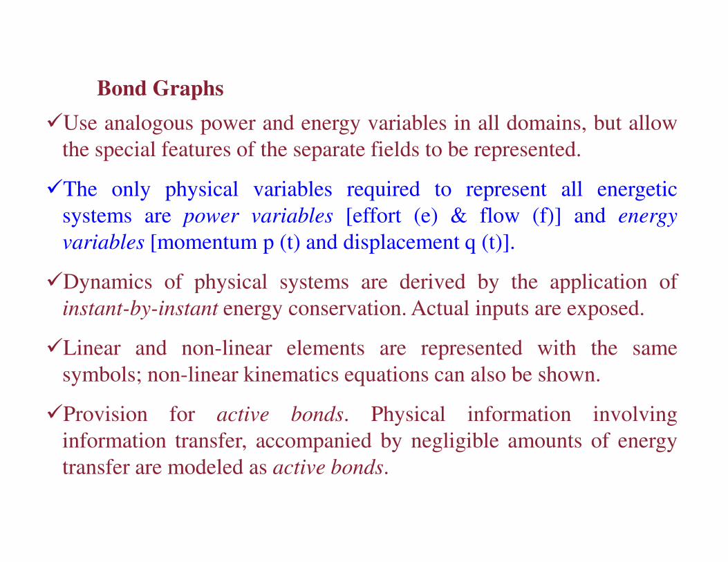
�Use analogous power and energy variables in all domains, but allow

the special features of the separate fields to be represented.

�The only physical variables required to represent all energetic

systems are power variables [effort (e) & flow (f)] and energy

variables [momentum p (t) and displacement q (t)].

�Dynamics of physical systems are derived by the application of

Bond Graphs

�Dynamics of physical systems are derived by the application of

instant-by-instant energy conservation. Actual inputs are exposed.

�Linear and non-linear elements are represented with the same

symbols; non-linear kinematics equations can also be shown.

�Provision for active bonds. Physical information involving

information transfer, accompanied by negligible amounts of energy

transfer are modeled as active bonds.

A Bond Graph’s Reach

Mechanical

Translation

Mechanical

Rotation

Hydraulic/Pneumatic

Electrical

Chemical/Process

Engineering

Thermal

Magnetic

Figure 2. Multi-Energy Systems Modeling using Bond Graphs

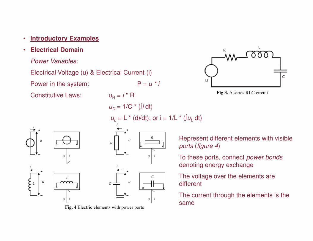
• Introductory Examples

• Electrical Domain

Power Variables:

Electrical Voltage (u) & Electrical Current (i)

Power in the system: P = u * i

Constitutive Laws: uR = i * R

uC = 1/C * (∫i dt)

uL = L * (di/dt); or i = 1/L * (∫uL dt)

Fig 3. A series RLC circuit

uL = L * (di/dt); or i = 1/L * (∫uL dt)

Fig. 4 Electric elements with power ports

Represent different elements with visible

ports (figure 4)

To these ports, connect power bonds

denoting energy exchange

The voltage over the elements are

different

The current through the elements is the

same

The R – L - C circuit

The common current becomes a “1-junction” in the bond graphs.

Note: the current through all connected bonds is the same, the voltages sum to zero

Fig 5. The RLC Circuit and its equivalent Bond Graph

1

Mechanical Domain

Mechanical elements like Force, Spring, Mass, Damper are similarly dealt with.

Power variables: Force (F) & Linear Velocity (v)

Power in the system: P = F * v

Constitutive laws: Fd = α * v Fs = KS * (∫v dt) = 1/CS * (∫ v dt)

Fm = m * (dv/dt); or v = 1/m * (∫Fm dt); Also, Fa = force

Fig 6. The Spring Mass Damper System and

its equivalent Bond Graph

The common velocity becomes a “1-junction” in the bond graphs. Note: the velocity of all

connected bonds is the same, the forces sum to zero)

Analogies Between The Mechanical And Electrical Elements

We see the following analogies

• The Damper is analogous to the Resistor.

• The Spring is analogous to the Capacitor, the mechanical compliance

corresponds with the electrical capacity.

• The Mass is analogous to the Inductor.• The Mass is analogous to the Inductor.

• The Force source is analogous to the Voltage source.

• The common Velocity is analogous to the loop Current.

� . Notice that the bond graphs of both the RLC circuit and the Spring-mass-damper system are identical

• Each of the various physical domains is characterized by a particular conserved quantity.

Table 1 illustrates these domains with corresponding flow (f), effort (e), generalized

displacement (q), and generalized momentum (p).

• Note that power = effort x flow in each case.

f

flow

e

effort

q = ∫f dt

generalized

displacement

p = ∫e dt

generalized

momentum

Electromagnetic i

current

u

voltage

q = ∫i dt

charge

λ = ∫u dt

magnetic flux linkage

Mechanical Translation

v

velocity

f

force

x = ∫v dt

displacement

p = ∫f dt

momentum

Mechanical Rotation ω T θ = ∫ω dt b = ∫T dt

Table 1. Domains with corresponding flow, effort, generalized displacement and generalized momentum

Mechanical Rotation ω

angular velocity

T

torque

θ = ∫ω dt

angular displacement

b = ∫T dt

angular momentum

Hydraulic / Pneumatic

φ

volume flow

P

pressure

V = ∫φ dt

volume

τ = ∫P dt

momentum of a flow tube

Thermal T

temperature

FS

entropy flow

S = ∫fS dt

entropy

Chemical µ

chemical potential

FN

molar flow

N = ∫fN dt

number of moles

� Bonds and Ports

Power port or port: The contact point of a sub model where

an ideal connection will be connected; location in a system

where energy transfer occurs

Power bond or bond: The connection between two sub models;

drawn by a single line

Bond denotes ideal energy flow between two sub models; the energy entering the

bond on one side immediately leaves the bond at the other side (power

A Be

f

(directed bond from A to B)

bond on one side immediately leaves the bond at the other side (power

continuity).

Fig. 7 Energy flow between two sub models represented by

ports and bonds [4]

�Energy flow along the bondhas the physical dimensionof power, being the productof two variables

Effort and Flow calledpower-conjugated variables

• Bond Graph Elements

Drawn as letter combinations (mnemonic codes) indicating the type of element.

C storage element for a q-type variable,

e.g. capacitor (stores charge), spring (stores displacement)

L storage element for a p-type variable,

e.g. inductor (stores flux linkage), mass (stores momentum)

R resistor dissipating free energy,

e.g. electric resistor, mechanical friction

Se, Sf sources,

e.g. electric mains (voltage source), gravity (force source),

pump (flow source)

TF transformer,

e.g. an electric transformer, toothed wheels, lever

GY gyrator,

e.g. electromotor, centrifugal pump

0, 1 0 and 1 junctions, for ideal connection of two or more sub-models

Storage Elements

Two types; C – elements & I – elements; q–type and p–type variables are conserved

quantities and are the result of an accumulation (or integration) process

C – element (capacitor, spring, etc.)

q is the conserved quantity, stored by accumulating the net flow, f to the storage element

Resulting balance equation dq/dt = f

Fig. 8 Examples of C - elements

An element relates effort to the generalized displacement

1-port element that stores and gives up energy without loss

I – element (inductor, mass, etc.)

p is the conserved quantity, stored by accumulating the net effort, e to the storage

element.

Resulting balance equation dp/dt = e

Fig. 9 Examples of I - elements

For an inductor, L [H] is the inductance and for a mass, m [kg] is the mass. For all other

domains, an I – element can be defined.

R – element (electric resistors, dampers, frictions, etc.)

R – elements dissipate free energy and energy flow towards the resistor is always positive.

Algebraic relation between effort and flow:e = r * (f)

Fig. 10 Examples of Resistors

If the resistance value can be controlled by an external signal, the resistor is a modulated

resistor, with mnemonic MR. E.g. hydraulic tap

Sources (voltage sources, current sources, external forces, ideal motors, etc.)

Sources represent the system-interaction with its environment. Depending on the type of the

imposed variable, these elements are drawn as Se or Sf.

Fig. 12 Examples of Sources [4]

Fig. 13 Example of Modulated Voltage

Source [4]

When a system part needs to be excited by a known signal form, the source can be modeled

by a modulated source driven by some signal form (figure 13).

Transformers (toothed wheel, electric transformer, etc.)

An ideal transformer is represented by TF and is power continuous (i.e. no power is stored or

dissipated). The transformations can be within the same domain (toothed wheel, lever) or

between different domains (electromotor, winch).

e1 = n * e2 & f2 = n * f1

Efforts are transduced to efforts and flows to flows; n is the transformer ratio.

Fig. 14 Examples of Transformers [4]

Gyrators (electromotor, pump, turbine)

An ideal gyrator is represented by GY and is power continuous (i.e. no power is stored or

dissipated). Real-life realizations of gyrators are mostly transducers representing a domain-

transformation.

e1 = r * f2 & e2 = r * f1

r is the gyrator ratio and is the only parameter required to describe both equations.

Fig. 15 Examples of Gyrators [4]

Junctions

Junctions couple two or more elements in a power continuous way; there is no storage or

dissipation at a junction.

0 – junction

Represents a node at which all efforts of the connecting bonds are equal. E.g. a parallel

connection in an electrical circuit.

The sum of flows of the connecting bonds is zero, considering the sign.

0 – junction can be interpreted as the generalized Kirchoff’s Current Law.

Equality of efforts (like electrical voltage) at a parallel connection.Equality of efforts (like electrical voltage) at a parallel connection.

Fig. 16 Example of a 0-Junction [4]

1 – junction

Is the dual form of the 0-junction (roles of effort and flow are exchanged).

Represents a node at which all flows of the connecting bonds are equal. E.g. a series

connection in an electrical circuit.

The efforts of the connecting bonds sum to zero.

1- junction can be interpreted as the generalized Kirchoff’s Voltage Law.

In the mechanical domain, 1-junction represents a force-balance, and is a generalization of

Newton’ third law.

Additionally, equality of flows (like electrical current) through a series connection.Additionally, equality of flows (like electrical current) through a series connection.

Fig. 17 Example of a 1-Junction [4]

Power Direction: The power is positive in the direction of the power

bond. If power is negative, it flows in the opposite direction of the

half-arrow.

Typical Power flow directions

R, C, and I elements have an incoming bond (half arrow towards the

element)

Se, Sf: outgoing bond

TF– and GY–elements (transformers and gyrators): one bond

incoming and one bond outgoing, to show the ‘natural’ flow of

energy.

These are constraints on the model!

• Causal Analysis

Causal analysis is the determination of the signal direction of the bonds

Establishes the cause and effect relationships between the bonds

Indicated in the bond graph by a causal stroke; the causal stroke indicates the direction of the

effort signal.

The result is a causal bond graph, which can be seen as a compact block diagram.

Fig. 18 Causality Assignment [4]

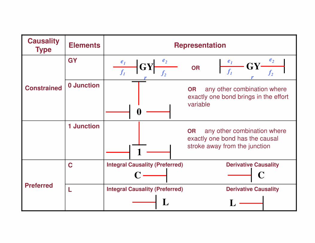
Causality

TypeElements Representation Interpretation

Fixed

Se

Sf

See

f

e

Se

f

Sfe

e

Sf

Causal Constraints: Four different types of constraints need to be discussed prior to

following a systematic procedure for bond graph formation and causal analysis

Constrained TF

OR

Sfe

fSf

f

TF

e1 e2

f2f1n

e1e2

f2f1

TFn

e1e2

f2f1

TFn

TF

e1 e2

f2f1n

Causality Type

Elements Representation

Constrained

GYOR

0 Junction

e1e2

f2f1

GYr

e1e2

f2f1

GYr

0

OR any other combination where

exactly one bond brings in the effort

variable

1 Junction

Preferred

C Integral Causality (Preferred) Derivative Causality

L Integral Causality (Preferred) Derivative Causality

1

OR any other combination where

exactly one bond has the causal

stroke away from the junction

CC

L L

Causality Type

Elements Representation

IndifferentR OR

R R

Some notes on Preferred Causality (C, I)

Causality determines whether an integration or differentiation w.r.t time is adopted in storage

elements. Integration has a preference over differentiation because:

1. At integrating form, initial condition must be specified.

2. Integration w.r.t. time can be realized physically; Numerical differentiation is not physically

realizable, since information at future time points is needed.

3. Another drawback of differentiation: When the input contains a step function, the output will

then become infinite.

Therefore, integrating causality is the preferred causality. C-element will have effort-out

causality and I-element will have flow-out causality

• Electrical Circuit # 1 (R-L-C) and its Bond Graph model

+

-

U0

U1U2

U3

Examples

0 0 0

0 1 0 1 0

U1 U2 U3

0: U12 0: U23

0: U12

0 1 0 1 0Se : UC : C

0: U23

R : R I : L

U1 U3U2

Examples (contd..)

1Se : U

C : C

R : R

I : L

Examples (contd..)

The Causality Assignment Algorithm:

1Se : U

C : C

R : R

I : L

1. 2.

1Se : U

C : C

R : R

I : L

C : C

1Se : U

C : C

R : R

I : L

3.

Examples (contd..)

• Electrical Circuit # 2 and its Bond Graph modelR1

R2R3

C1

C2

L1

R1 R2 R3

C2C1L1

• A DC Motor and its Bond Graph model