Page 1
ADVANCED BIOENGINEERING METHODS LABORATORY
BROWNIAN MOTION AND SINGLE PARTICLE TRACKING
Aleksandra Radenovic
1
BROWNIAN MOTION AND
SINGLE PARTICLE TRACKING
ABSTRACT
This lab begins with the ground-breaking physics of a century ago demonstrating the atomic nature of
matter and ends with todays biophysics state-of-the-art of intracellular transport and molecular motors
The pairing of advanced light microscopy with automated image analysis and particle tracking software
provides a powerful tool for investigating the motion of molecules organelles and cells In the first part
of this lab Perrins work will be replicated with such modern equipments the motion of synthetic beads
suspended in liquids of various viscosities will be tracked and studied In the second part the motion of
particles inside living cells will be observed Thereby this practical will introduce the bases of bead
suspension sample preparation microscopy aspects particle detection and tracking as well as data
analysis using matlab
ADVANCED BIOENGINEERING METHODS LABORATORY
BROWNIAN MOTION AND SINGLE PARTICLE TRACKING
Aleksandra Radenovic
2
TABLE OF CONTENTS
1 Theory 3
11 What is Brownian motion 3
12 Calculation of the Mean Square Displacement 4
13 Intracellular Transport 6
2 Practical work 10
21 Material requirements 10
22 Calibration and Testing 10
23 Viscous suspensions preparation 11
24 Polystyrene suspensions preparation 11
25 Polystyrene suspensions preparation 11
26 Slide loading 12
27 View the slide in transmitted light 13
28 Set-up darkfield illumination 13
29 Viewing Tracking Particles in Viscous Suspensions 13
210 Making an onion slide 15
211 Making observations 16
3 Data analysis 17
31 Calibration 17
32 Particle Tracking 17
33 Matlab analysis 22
34 Questions 23
4 References 23
ADVANCED BIOENGINEERING METHODS LABORATORY
BROWNIAN MOTION AND SINGLE PARTICLE TRACKING
Aleksandra Radenovic
3
Please find the exercise on Brownian motion simulation on the web
site and please do it at home before the practical session
1 THEORY
11 What is Brownian motion
Although it was Jan Ingenhousz who made the first known documented observations of fluctuating
movements of carbon dust particles in alcohol in 1765 the discovery of Brownian motion is credited to
Robert Brown due to his observations of pollen in water in 1827 Also because the previous description
by Ingenhousz was not well known the chaotic movement was for a long time considered to be a
property of living or at least organic matter Brownian motion is stochastic movements of small particles
suspended in a solution The molecules (for example water molecules) constituting the fluid constantly hit
the immersed objects which results in chaotic and non-directed movements These movements can be
measured by the mean square displacement 2
r and the lag time t and is characterized by the
diffusion coefficient D which is a measure of the speed of diffusion For three-dimensional brownian
motions these terms can be put into an equation as follows
2
6r D t (01)
This is only true for isotropic and unrestricted translational diffusion Brownian motion is actually
observed for many different dynamical phenomena Here we concentrate on isotropic translational
displacements (random walk) but brownian motion can be also of rotational undulating etc nature
Translational diffusion or random walk in three dimensions can mathematically be described by a
differential equation
( )
( )r
D rt
(02)
Where ( )r is the particle location distribution and ∆ is the Laplace-Operator which is a second order
differential operator
In 1905 Einstein published a paper that predicted a relationship between the mean squared magnitude of
Brownian excursions and the size of molecules 1-2
Now all that remained was to do the experiment Jean
Perrin 3-5
won the Nobel Prize in 1926 for his work confirming Einsteins hypothesis Perrins
experimental confirmation of Einsteins equation was an important piece of evidence to help settle a
debate about the nature of mater that had begun nearly 2000 years earlier in the time of Democritus and
Anaxagoras Since then a thorough understanding of Brownian motion has become essential for diverse
fields are ranging from polymer physics to biophysics aerodynamics to statistical mechanics and even
stock option pricing
Albert Einstein has calculated the diffusion coefficient to for a spherical particle
3
Bk TD
d
(03)
ADVANCED BIOENGINEERING METHODS LABORATORY
BROWNIAN MOTION AND SINGLE PARTICLE TRACKING
Aleksandra Radenovic
4
where kB is the Boltzmann constant T the temperature η the viscosity of the medium and d the diameter
of the diffusing particle The dimension of the diffusion coefficient is m2s The given relation between
diffusion coefficient temperature viscosity and particle size is only true for isotropic non-hindered
diffusion of a spherical particle The diffusion coefficient therefore gives us information about the
temperature and viscosity of the system and size and shape of the diffusing particle
For two and one dimensions the time dependence of mean square displacements for isotropic diffusion
differs only in the numerical factor
2
2
dim 4
dim 2
two r D t
one x D t
(04)
The diffusion coefficient does not depend on the dimensions in which the diffusion takes place
Hindered or restricted diffusion is for example the case where the particle has to diffuse in a porous or
structured environment as in cells Anisotropic diffusion takes place in cases when the particle itself has
an asymmetric shape Then the diffusion coefficient is no simple scalar like in eq03 anymore but
becomes a complex tensor
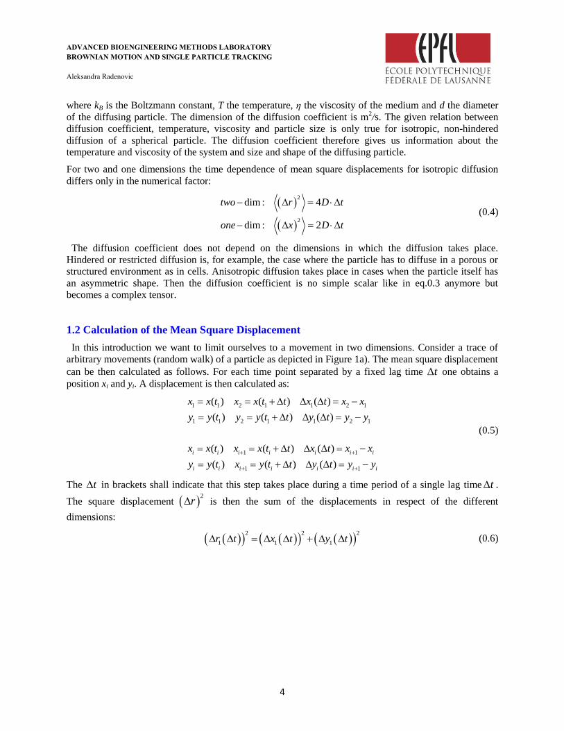
12 Calculation of the Mean Square Displacement
In this introduction we want to limit ourselves to a movement in two dimensions Consider a trace of
arbitrary movements (random walk) of a particle as depicted in Figure 1a) The mean square displacement
can be then calculated as follows For each time point separated by a fixed lag time t one obtains a
position xi and yi A displacement is then calculated as
1 1 2 1 1 2 1
1 1 2 1 1 2 1
1 1
1 1
( ) ( ) ( )
( ) ( ) ( )
( ) ( ) ( )
( ) ( ) ( )
i i i i i i i
i i i i i i i
x x t x x t t x t x x
y y t y y t t y t y y
x x t x x t t x t x x
y y t x y t t y t y y
(05)
The t in brackets shall indicate that this step takes place during a time period of a single lag time t
The square displacement 2
r is then the sum of the displacements in respect of the different
dimensions
2 2 2
1 1 1r t x t y t (06)
ADVANCED BIOENGINEERING METHODS LABORATORY
BROWNIAN MOTION AND SINGLE PARTICLE TRACKING
Aleksandra Radenovic
5
Figure 1 a) Random walk in 2D intermediate positions and traces of a diffusing particle Continuous lines indicate the
displacement corresponding to single steps dotted lines to double step during two time intervals b) Squared displacements can
be plotted according to the time intervals Note that for longer steps the number of data points becomes less c) Data points
corresponding to one time interval merge into on average value Fitting should give a straight line for unrestricted and isotropic
diffusion
Q1 Note that the error bar becomes larger for larger steps Why
The displacement and the square displacement can be calculated for every step of the same trace
corresponding to the same step size of stepping time (step during the time length t )
2 2 2
2 2
2 2 2
3 3 3
2 2 2
2
i i i
r t x t y t
r t x t y t
r t x t y t
(07)
The mean square displacement is obtained as an average of all steps corresponding to a single lag time
t
2 2 2 2 2
1 2 1
1
1 1( ) ( ) ( ) ( ) ( )
n
i
i
r t r t r t r t r tn n
(08)
The same procedure applies to double step during a time length of 2 t
Q2 Please provide step by step calculation for 2 t and 3 t
Now the mean square displacement (MSD) can be plotted to its corresponding step time interval which
gives characteristic curves If the analyzed diffusion is of isotropic nature then one would expect a linear
correlation In this case the slope of the line corresponds to the diffusion coefficient multiplied with its
factor (normally 2 4 or 6) Diffusion or random walk can be hindered or restricted which changes the
characteristic form of the MSD plots In the case of diffusion restricted to a confined space the MSD
ADVANCED BIOENGINEERING METHODS LABORATORY
BROWNIAN MOTION AND SINGLE PARTICLE TRACKING
Aleksandra Radenovic
6
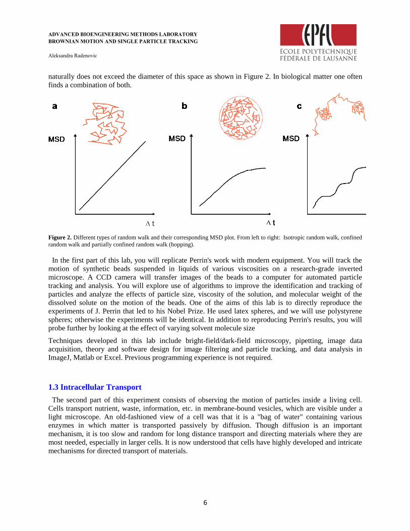
naturally does not exceed the diameter of this space as shown in Figure 2 In biological matter one often
finds a combination of both
Figure 2 Different types of random walk and their corresponding MSD plot From left to right Isotropic random walk confined
random walk and partially confined random walk (hopping)
In the first part of this lab you will replicate Perrins work with modern equipment You will track the
motion of synthetic beads suspended in liquids of various viscosities on a research-grade inverted
microscope A CCD camera will transfer images of the beads to a computer for automated particle
tracking and analysis You will explore use of algorithms to improve the identification and tracking of
particles and analyze the effects of particle size viscosity of the solution and molecular weight of the
dissolved solute on the motion of the beads One of the aims of this lab is to directly reproduce the
experiments of J Perrin that led to his Nobel Prize He used latex spheres and we will use polystyrene
spheres otherwise the experiments will be identical In addition to reproducing Perrins results you will
probe further by looking at the effect of varying solvent molecule size
Techniques developed in this lab include bright-fielddark-field microscopy pipetting image data
acquisition theory and software design for image filtering and particle tracking and data analysis in
ImageJ Matlab or Excel Previous programming experience is not required
13 Intracellular Transport
The second part of this experiment consists of observing the motion of particles inside a living cell
Cells transport nutrient waste information etc in membrane-bound vesicles which are visible under a
light microscope An old-fashioned view of a cell was that it is a bag of water containing various
enzymes in which matter is transported passively by diffusion Though diffusion is an important
mechanism it is too slow and random for long distance transport and directing materials where they are
most needed especially in larger cells It is now understood that cells have highly developed and intricate
mechanisms for directed transport of materials
ADVANCED BIOENGINEERING METHODS LABORATORY
BROWNIAN MOTION AND SINGLE PARTICLE TRACKING
Aleksandra Radenovic
7
a b
c
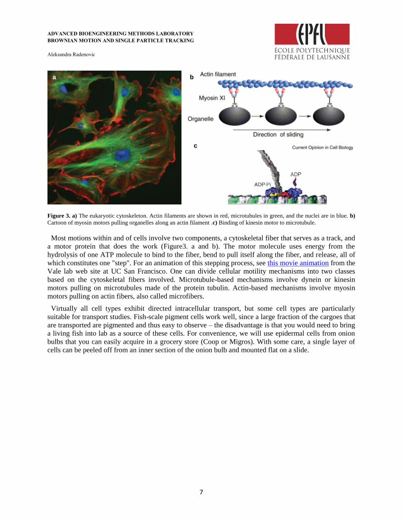
Figure 3 a) The eukaryotic cytoskeleton Actin filaments are shown in red microtubules in green and the nuclei are in blue b)
Cartoon of myosin motors pulling organelles along an actin filament c) Binding of kinesin motor to microtubule
Most motions within and of cells involve two components a cytoskeletal fiber that serves as a track and
a motor protein that does the work (Figure3 a and b) The motor molecule uses energy from the
hydrolysis of one ATP molecule to bind to the fiber bend to pull itself along the fiber and release all of
which constitutes one step For an animation of this stepping process see this movie animation from the
Vale lab web site at UC San Francisco One can divide cellular motility mechanisms into two classes
based on the cytoskeletal fibers involved Microtubule-based mechanisms involve dynein or kinesin
motors pulling on microtubules made of the protein tubulin Actin-based mechanisms involve myosin
motors pulling on actin fibers also called microfibers
Virtually all cell types exhibit directed intracellular transport but some cell types are particularly
suitable for transport studies Fish-scale pigment cells work well since a large fraction of the cargoes that
are transported are pigmented and thus easy to observe ndash the disadvantage is that you would need to bring
a living fish into lab as a source of these cells For convenience we will use epidermal cells from onion
bulbs that you can easily acquire in a grocery store (Coop or Migros) With some care a single layer of
cells can be peeled off from an inner section of the onion bulb and mounted flat on a slide
ADVANCED BIOENGINEERING METHODS LABORATORY
BROWNIAN MOTION AND SINGLE PARTICLE TRACKING
Aleksandra Radenovic
8
a b
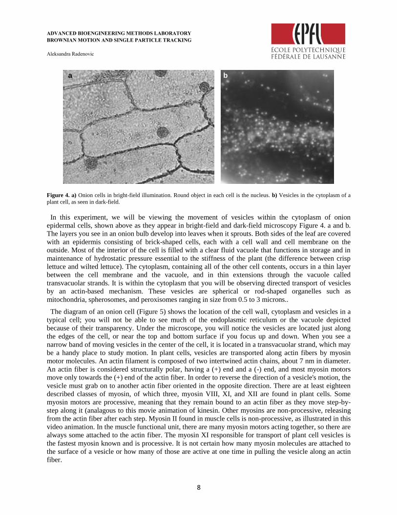
Figure 4 a) Onion cells in bright-field illumination Round object in each cell is the nucleus b) Vesicles in the cytoplasm of a
plant cell as seen in dark-field
In this experiment we will be viewing the movement of vesicles within the cytoplasm of onion
epidermal cells shown above as they appear in bright-field and dark-field microscopy Figure 4 a and b
The layers you see in an onion bulb develop into leaves when it sprouts Both sides of the leaf are covered
with an epidermis consisting of brick-shaped cells each with a cell wall and cell membrane on the
outside Most of the interior of the cell is filled with a clear fluid vacuole that functions in storage and in
maintenance of hydrostatic pressure essential to the stiffness of the plant (the difference between crisp
lettuce and wilted lettuce) The cytoplasm containing all of the other cell contents occurs in a thin layer
between the cell membrane and the vacuole and in thin extensions through the vacuole called
transvacuolar strands It is within the cytoplasm that you will be observing directed transport of vesicles
by an actin-based mechanism These vesicles are spherical or rod-shaped organelles such as
mitochondria spherosomes and peroxisomes ranging in size from 05 to 3 microns
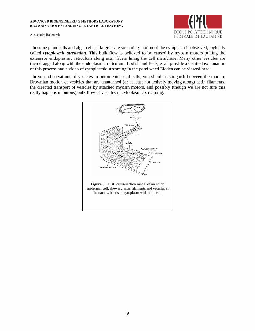
The diagram of an onion cell (Figure 5) shows the location of the cell wall cytoplasm and vesicles in a
typical cell you will not be able to see much of the endoplasmic reticulum or the vacuole depicted
because of their transparency Under the microscope you will notice the vesicles are located just along
the edges of the cell or near the top and bottom surface if you focus up and down When you see a
narrow band of moving vesicles in the center of the cell it is located in a transvacuolar strand which may
be a handy place to study motion In plant cells vesicles are transported along actin fibers by myosin
motor molecules An actin filament is composed of two intertwined actin chains about 7 nm in diameter
An actin fiber is considered structurally polar having a (+) end and a (-) end and most myosin motors
move only towards the (+) end of the actin fiber In order to reverse the direction of a vesicles motion the
vesicle must grab on to another actin fiber oriented in the opposite direction There are at least eighteen
described classes of myosin of which three myosin VIII XI and XII are found in plant cells Some
myosin motors are processive meaning that they remain bound to an actin fiber as they move step-by-
step along it (analagous to this movie animation of kinesin Other myosins are non-processive releasing
from the actin fiber after each step Myosin II found in muscle cells is non-processive as illustrated in this
video animation In the muscle functional unit there are many myosin motors acting together so there are
always some attached to the actin fiber The myosin XI responsible for transport of plant cell vesicles is
the fastest myosin known and is processive It is not certain how many myosin molecules are attached to
the surface of a vesicle or how many of those are active at one time in pulling the vesicle along an actin
fiber
ADVANCED BIOENGINEERING METHODS LABORATORY
BROWNIAN MOTION AND SINGLE PARTICLE TRACKING
Aleksandra Radenovic
9
In some plant cells and algal cells a large-scale streaming motion of the cytoplasm is observed logically
called cytoplasmic streaming This bulk flow is believed to be caused by myosin motors pulling the
extensive endoplasmic reticulum along actin fibers lining the cell membrane Many other vesicles are
then dragged along with the endoplasmic reticulum Lodish and Berk et al provide a detailed explanation
of this process and a video of cytoplasmic streaming in the pond weed Elodea can be viewed here
In your observations of vesicles in onion epidermal cells you should distinguish between the random
Brownian motion of vesicles that are unattached (or at least not actively moving along) actin filaments
the directed transport of vesicles by attached myosin motors and possibly (though we are not sure this
really happens in onions) bulk flow of vesicles in cytoplasmic streaming
Figure 5 A 3D cross-section model of an onion
epidermal cell showing actin filaments and vesicles in
the narrow bands of cytoplasm within the cell
ADVANCED BIOENGINEERING METHODS LABORATORY
BROWNIAN MOTION AND SINGLE PARTICLE TRACKING
Aleksandra Radenovic
10
2 PRACTICAL WORK
21 Material requirements
Handling Safety glasses gloves tweezers pipettes spoons razor blades scalpels
Machines IX 71 microscope dark field bright field Pipettor Finpette 10-100μL
Products Synthetic beads from Bangs Laboratories httpwwwbangslabscom (1041μm)
Solvents Glycerol PBS water
Please read the microscopy part as well as the Koehlerdark field illumination part of
the master handout BEFORE using the microscopy
22 Calibration and Testing (done by TA beforehand)
Before taking data in your first investigation you must calibrate the microscope and learn the
experimental techniques involving pipetting microscopy and data-taking Your first slide preparation of
10μm beads will be used to determine the conversion from pixels in the image to μm on the actual
specimen This calibration must be done separately for the microscopes 20x objective lens and 40x
objective lens For testing purposes you will make a slide of 1μm beads in water set up dark-field
illumination on the microscope and experiment with settings of the lighting focus and particle tracker
software to successfully track beads and save data on particle motion Setting up bright-field Kohler
illumination and dark-field illumination requires careful alignment and some practice but this will pay off
later in the quality of your images and data
23 Viscous suspensions preparation
A solution will consist of three parts PBS buffer which makes up most of the solution a solute glycerol
to provide the viscosity and the beads which we will then observe PBS buffer together with glycerol and
beads solution is located in the 4 degC in the fridge and are also clearly marked Note that the glycerol is
extremely sticky (ie viscous) and will not be measured precisely using the pipette as it will stick to both
the inside and outside of the filter tip To measure glycerol it is best to use the scale located at the lab
station Note (11 ratio water glycerol (labeled 50 glycerol by weight) 12 (labeled 75 glycerol by
weight) are also located in the 4 degC fridge
Use the table below to compute the required dilution of the solvent The stock Glycerol is a thick liquid
with gt99 purity It will require some care to measure the pure glycerol accurately since it tends to stick
to the sides of the pipette tip For this reason weighing the glycerol before adding the water is probably a
better technique than adding the glycerol to the water You may either use these values or interpolate
between them
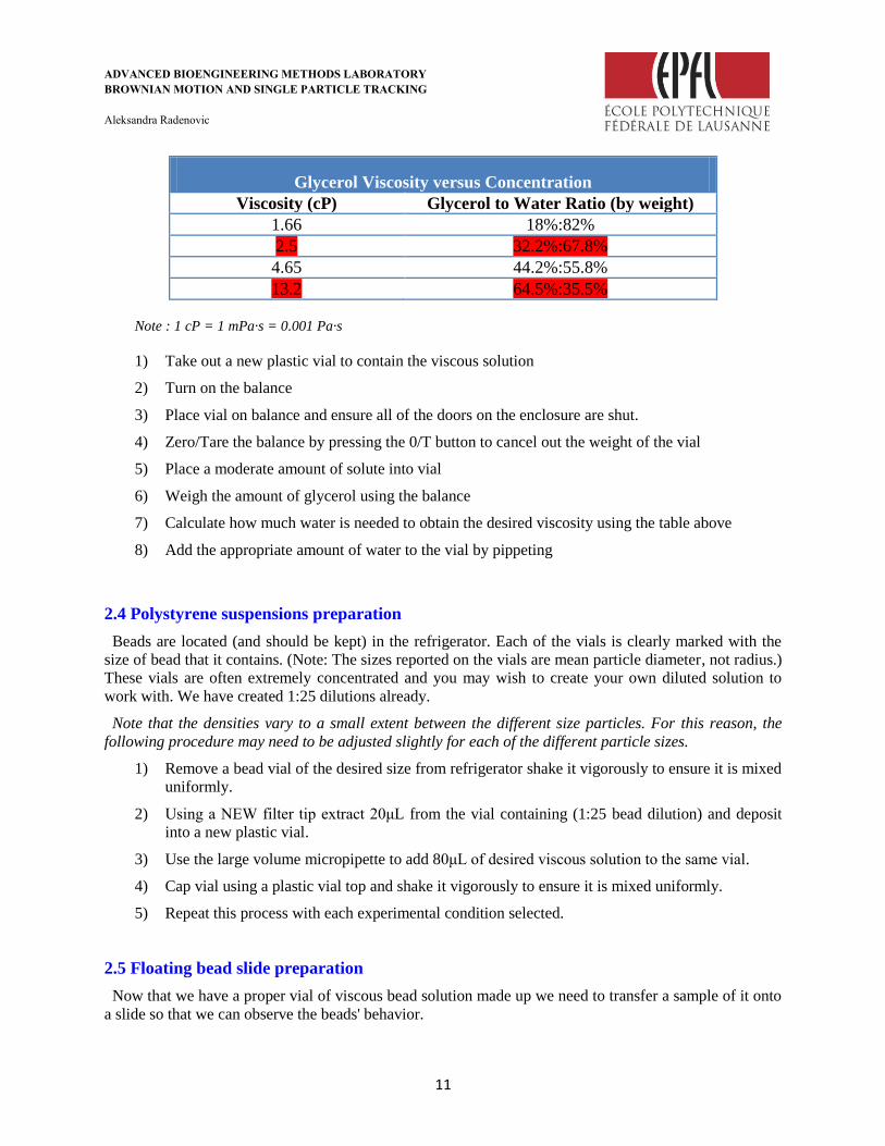
PLEASE do ONLY 3 different viscosities pure water and the other two marked in red
ADVANCED BIOENGINEERING METHODS LABORATORY
BROWNIAN MOTION AND SINGLE PARTICLE TRACKING
Aleksandra Radenovic
11
Glycerol Viscosity versus Concentration
Viscosity (cP) Glycerol to Water Ratio (by weight)
166 1882
25 322678
465 442558
132 645355
Note 1 cP = 1 mPamiddots = 0001 Pamiddots
1) Take out a new plastic vial to contain the viscous solution
2) Turn on the balance
3) Place vial on balance and ensure all of the doors on the enclosure are shut
4) ZeroTare the balance by pressing the 0T button to cancel out the weight of the vial
5) Place a moderate amount of solute into vial
6) Weigh the amount of glycerol using the balance
7) Calculate how much water is needed to obtain the desired viscosity using the table above
8) Add the appropriate amount of water to the vial by pippeting
24 Polystyrene suspensions preparation
Beads are located (and should be kept) in the refrigerator Each of the vials is clearly marked with the
size of bead that it contains (Note The sizes reported on the vials are mean particle diameter not radius)
These vials are often extremely concentrated and you may wish to create your own diluted solution to
work with We have created 125 dilutions already
Note that the densities vary to a small extent between the different size particles For this reason the
following procedure may need to be adjusted slightly for each of the different particle sizes
1) Remove a bead vial of the desired size from refrigerator shake it vigorously to ensure it is mixed
uniformly
2) Using a NEW filter tip extract 20μL from the vial containing (125 bead dilution) and deposit
into a new plastic vial
3) Use the large volume micropipette to add 80μL of desired viscous solution to the same vial
4) Cap vial using a plastic vial top and shake it vigorously to ensure it is mixed uniformly
5) Repeat this process with each experimental condition selected
25 Floating bead slide preparation
Now that we have a proper vial of viscous bead solution made up we need to transfer a sample of it onto
a slide so that we can observe the beads behavior
ADVANCED BIOENGINEERING METHODS LABORATORY
BROWNIAN MOTION AND SINGLE PARTICLE TRACKING
Aleksandra Radenovic
12
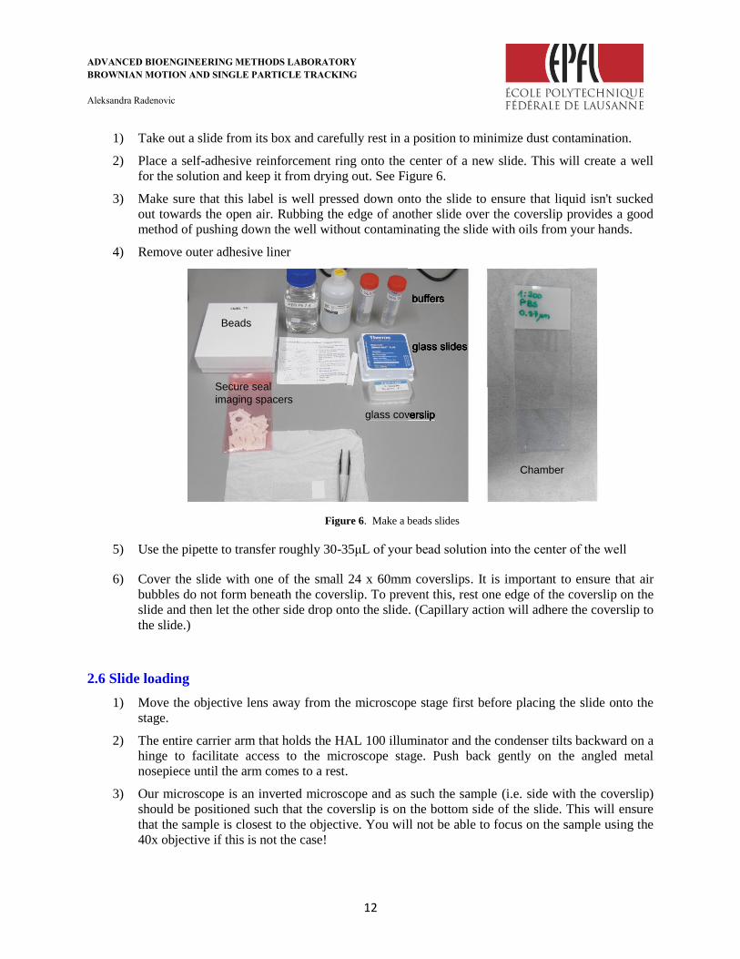
1) Take out a slide from its box and carefully rest in a position to minimize dust contamination
2) Place a self-adhesive reinforcement ring onto the center of a new slide This will create a well
for the solution and keep it from drying out See Figure 6
3) Make sure that this label is well pressed down onto the slide to ensure that liquid isnt sucked
out towards the open air Rubbing the edge of another slide over the coverslip provides a good
method of pushing down the well without contaminating the slide with oils from your hands
4) Remove outer adhesive liner
Secure seal
imaging spacers
Beads
glass coverslip
glass slides
buffers
Chamber
Figure 6 Make a beads slides
5) Use the pipette to transfer roughly 30-35μL of your bead solution into the center of the well
6) Cover the slide with one of the small 24 x 60mm coverslips It is important to ensure that air
bubbles do not form beneath the coverslip To prevent this rest one edge of the coverslip on the
slide and then let the other side drop onto the slide (Capillary action will adhere the coverslip to
the slide)
26 Slide loading
1) Move the objective lens away from the microscope stage first before placing the slide onto the
stage
2) The entire carrier arm that holds the HAL 100 illuminator and the condenser tilts backward on a
hinge to facilitate access to the microscope stage Push back gently on the angled metal
nosepiece until the arm comes to a rest
3) Our microscope is an inverted microscope and as such the sample (ie side with the coverslip)
should be positioned such that the coverslip is on the bottom side of the slide This will ensure
that the sample is closest to the objective You will not be able to focus on the sample using the
40x objective if this is not the case
ADVANCED BIOENGINEERING METHODS LABORATORY
BROWNIAN MOTION AND SINGLE PARTICLE TRACKING
Aleksandra Radenovic
13
27 View the slide in transmitted light
In this step you will view your sample under Koumlhler illumination to achieve uniform illumination with
little reflection or glare and minimal sample heating Please find the Koehler illumination protocol in the
master handout
The samples in this lab are difficult to focus on because they have very little contrast If you have trouble
focusing try starting with the 10x objective At higher magnification it is sometimes helpful to focus on
the edge of the slide first to get the setting close
SAFETY (MICROSCOPE MANIPULATION)
Stay away from slower particles for they are close to the edges The eyepieces are designed to be used
while wearing eyeglasses If you do not wear glasses DO NOT get too close to them
28 Set-up darkfield illumination
Now you can set up the dark field illumination Please find the Dark field illumination protocol in the
master handout
1) Select the 20x objective and establish the Koehler illumination
2) Set the dark field illumination
3) Open the field iris all the way
4) Increase the light intensity using the Toggle Switch for Illumination Intensity You will need to
turn the light level up significantly in order to see the small amount of light scattered by the
smaller nanoparticles (even though the PS spheres will be easily visible)
29 Viewing Tracking Particles in Viscous Suspensions
Now that suspensions and sample chambers have been made for each experimental condition and the
microscope has been fully configured we are now ready to take data
1) Use 10μm beads sample to establish the pixel size of your camera (already done by your TA)
2) Turn on the Andor camera
3) Open Andor camera software called Solis
4) Turn the switch on the microscope to send an image to CCD camera
5) Click on the movie camera icon to get a live image from your sample
6) Set up the exposure time to 005s by pressing exposure button (Figure 7)
7) To take pixel calibration image open in the main menu acquisition under setup CCD select
Single and enter the following value exposure time 001-0075s Then under Setup acquisition
open binning to 512-512 pixels you can move binning box to the region around your 10m
bead press Ok and close Acquisition menu
8) Press Record and save image as sif file
ADVANCED BIOENGINEERING METHODS LABORATORY
BROWNIAN MOTION AND SINGLE PARTICLE TRACKING
Aleksandra Radenovic
14
RecordLive Exposure
Figure 7 Andor Solis program for data acquisition Bright field image of 097 m beads
9) Watch out for bulk flow If you see a number of particles moving in one direction they are
likely undergoing bulk flow This could be due to evaporation of liquid from beneath the
coverslip or an air bubble popping or various other conditions If you see bulk flow occuring
your data will be skewed MAKE SURE there is no bulk flow when collecting data
10) Now we are ready to collect movies for your analysis session
11) To setup your movies exposure time t kinetic series length (number of frames in your
movies ) open in the main menu acquisition under setup CCD select Kinetic series enter
following values exposure time 001-01s kinetic series length 200 next under Setup
acquisition open binning to 512-512 pixels you can move binning box to the region containing
the most beads Mark in your notebook the values you entered
12) Press record
13) Save files as sif Collect all necessary data and save them in your folder
14) Repeat this for each experimental condition selected select three viscosities for 097 m beads
15) Once you have finished data collection you will need to convert all sif files in raw files You
can do it file by file or using a batch conversion option in File menu (Main Menu) Make sure
ADVANCED BIOENGINEERING METHODS LABORATORY
BROWNIAN MOTION AND SINGLE PARTICLE TRACKING
Aleksandra Radenovic
15
that you convert it in 16 bit unsigned integer (with range 0-65322) This is format required for
the analysis session
16) For those of you interested in a challenge you can attempt to create a program in C++ or
Matlab to adjust for bulk flow in the slide
17) If you have enough time repeat this experiment for other bead size or add one more viscosity
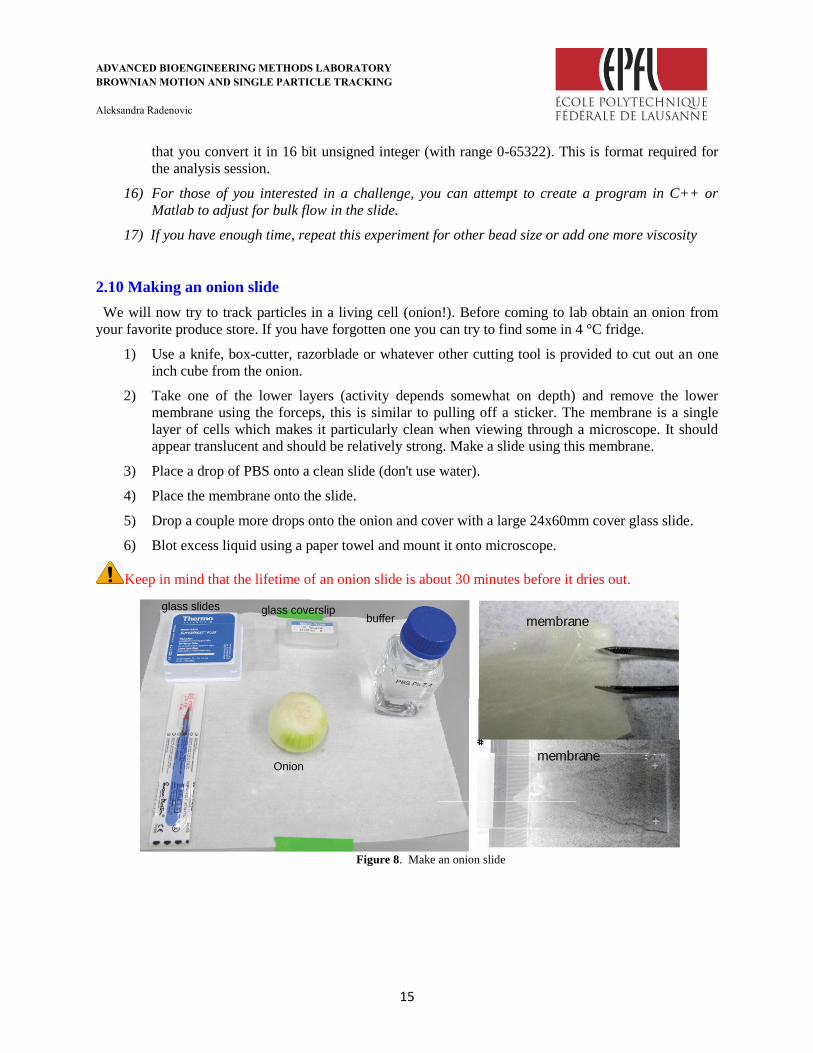
210 Making an onion slide
We will now try to track particles in a living cell (onion) Before coming to lab obtain an onion from
your favorite produce store If you have forgotten one you can try to find some in 4 degC fridge
1) Use a knife box-cutter razorblade or whatever other cutting tool is provided to cut out an one
inch cube from the onion
2) Take one of the lower layers (activity depends somewhat on depth) and remove the lower
membrane using the forceps this is similar to pulling off a sticker The membrane is a single
layer of cells which makes it particularly clean when viewing through a microscope It should
appear translucent and should be relatively strong Make a slide using this membrane
3) Place a drop of PBS onto a clean slide (dont use water)
4) Place the membrane onto the slide
5) Drop a couple more drops onto the onion and cover with a large 24x60mm cover glass slide
6) Blot excess liquid using a paper towel and mount it onto microscope
Keep in mind that the lifetime of an onion slide is about 30 minutes before it dries out
Onion
glass coverslipglass slidesbuffer membrane
membrane
Figure 8 Make an onion slide
ADVANCED BIOENGINEERING METHODS LABORATORY
BROWNIAN MOTION AND SINGLE PARTICLE TRACKING
Aleksandra Radenovic
16
211Making Observations
First you should spend a little while looking around trying to find some regions of interest Note the
different types of movement and where they tend to occur In particular be sure to investigate regions
around the cell walls around the nucleus and also see if you can find anything happening within the
otherwise empty center of the cell Most of the activity happens on the lower and upper layers of the cell
as the center is occupied with the vacuole which should be devoid of anything except water If you scan
through the depths of a few cells carefully (using the focus knob to move in depth) you should be able to
find isolated actin fibers which make for very clean data-taking Your data analysis will be much easier if
you can isolate the forms of movement within the cell and only take data on one type at a time
If you dont find much activity you could try a different section of onion or another onion altogether
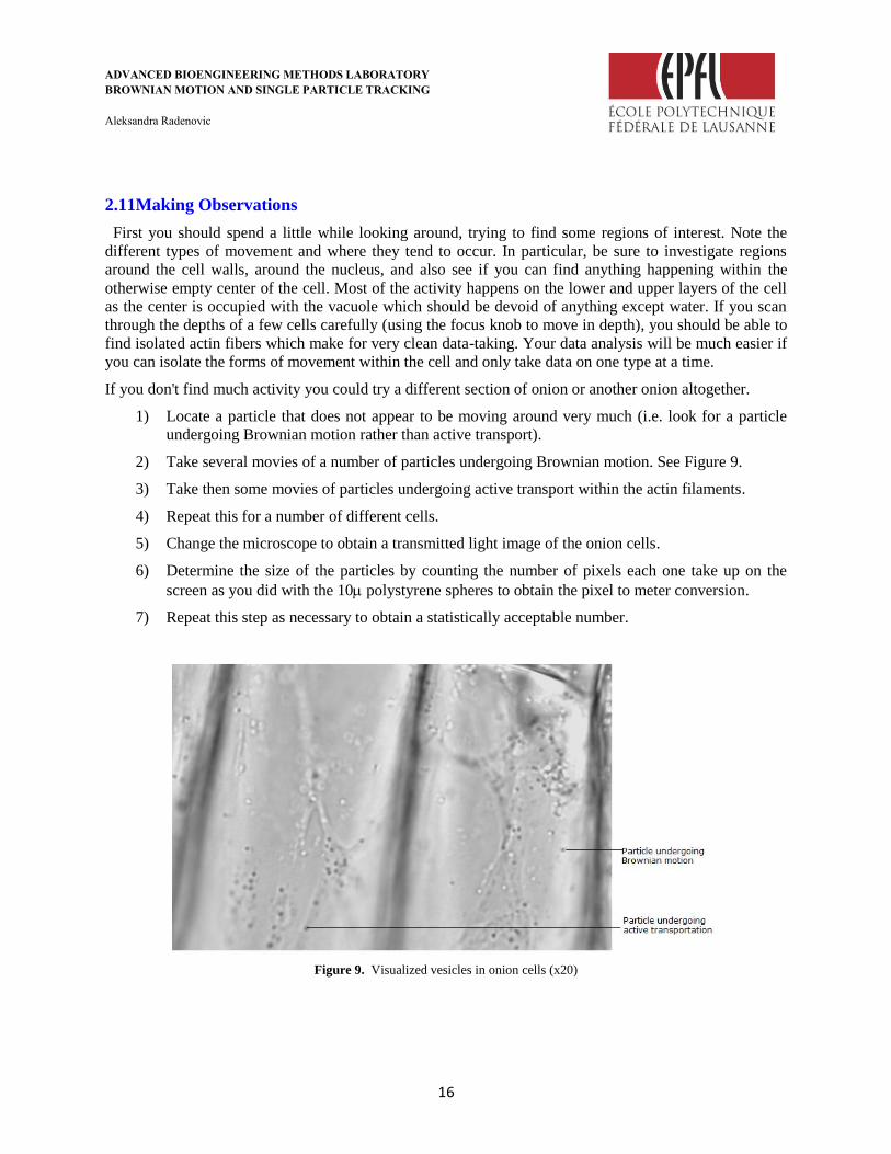
1) Locate a particle that does not appear to be moving around very much (ie look for a particle
undergoing Brownian motion rather than active transport)
2) Take several movies of a number of particles undergoing Brownian motion See Figure 9
3) Take then some movies of particles undergoing active transport within the actin filaments
4) Repeat this for a number of different cells
5) Change the microscope to obtain a transmitted light image of the onion cells
6) Determine the size of the particles by counting the number of pixels each one take up on the
screen as you did with the 10 polystyrene spheres to obtain the pixel to meter conversion
7) Repeat this step as necessary to obtain a statistically acceptable number
Figure 9 Visualized vesicles in onion cells (x20)
ADVANCED BIOENGINEERING METHODS LABORATORY
BROWNIAN MOTION AND SINGLE PARTICLE TRACKING
Aleksandra Radenovic
17
3 DATA ANALYSIS
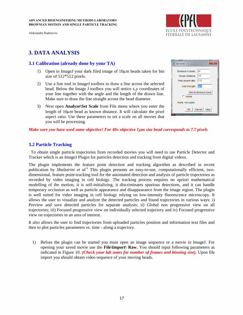
31 Calibration (already done by your TA)
1) Open in ImageJ your dark filed image of 10m beads taken for bin
size of 512512 pixels
2) Use a line tool in ImageJ toolbox to draw a line across the selected
bead Below the Image J toolbox you will notice xy coordinates of
your line together with the angle and the length of the drawn line
Make sure to draw the line straight across the bead diameter
3) Next open AnalyzeSet Scale from File menu where you enter the
length of 10m bead as known distance It will calculate the pixel
aspect ratio Use these parameters to set a scale on all movies that
you will be processing
Make sure you have used same objective For 40x objective 1m size bead corresponds to 77 pixels
32 Particle Tracking
To obtain single particle trajectories from recorded movies you will need to use Particle Detector and
Tracker which is an ImageJ Plugin for particles detection and tracking from digital videos
The plugin implements the feature point detection and tracking algorithm as described in recent
publication by Sbalzarini et al6 This plugin presents an easy-to-use computationally efficient two-
dimensional feature point-tracking tool for the automated detection and analysis of particle trajectories as
recorded by video imaging in cell biology The tracking process requires no apriori mathematical
modelling of the motion it is self-initializing it discriminates spurious detections and it can handle
temporary occlusion as well as particle appearance and disappearance from the image region The plugin
is well suited for video imaging in cell biology relying on low-intensity fluorescence microscopy It
allows the user to visualize and analyze the detected particles and found trajectories in various ways i)
Preview and save detected particles for separate analysis ii) Global non progressive view on all
trajectories iii) Focused progressive view on individually selected trajectory and iv) Focused progressive
view on trajectories in an area of interest
It also allows the user to find trajectories from uploaded particles position and information text files and
then to plot particles parameters vs time - along a trajectory
1) Before the plugin can be started you must open an image sequence or a movie in ImageJ For
opening your saved movie use the FileImport Raw You should input following parameters as
indicated in Figure 10 (Check your lab notes for number of frames and binning size) Upon file
import you should obtain video sequence of your moving beads
ADVANCED BIOENGINEERING METHODS LABORATORY
BROWNIAN MOTION AND SINGLE PARTICLE TRACKING
Aleksandra Radenovic
18
Figure 10 Import parameters
2) Next you need to improve contrast and adapt your movie so that it can be treated with
ParticleTracker plugin To do so use the ImageType 8 bit option from File menu Next you need
to increase contrast you will do it by using ProcessEnhance Contrast option from File menu It is
safe to select 01saturated pixels under Use Stack Histogram see Figure 11 To filter out noise
use ProcessFilterGaussian blur option from File menu Again safe sigma value to use is
12Befor aoplying this filtering you can preview your movie
Figure 11 Parameters for better movie quality
3) Now that the movie is open and compatible with the plugging you can start the plugin by
selecting ParticleTracker from the Plugins - Particle Detector amp Tracker menu After starting the
plugin a dialog screen is displayed The dialog has two parts ldquoParticle Detectionrdquo and ldquoParticle
Linkingrdquo
Particle Detection This part of the dialog allows you to adjust parameters relevant to the
particle detection (feature point detection) part of the algorithm
ADVANCED BIOENGINEERING METHODS LABORATORY
BROWNIAN MOTION AND SINGLE PARTICLE TRACKING
Aleksandra Radenovic
19
Preview the detected particles in each frame according to the parameters This options offers
assistance in choosing good values for the parameters Save the detected particles according to
the parameters for all frames The parameters relevant for detection are
Radius Approximate radius of the particles in the images in units of pixels The value should
be slightly larger than the visible particle radius but smaller than the smallest inter-particle
separation
Cutoff The score cut-off for the non-particle discrimination
Percentile The percentile (r) that determines which bright pixels are accepted as Particles All
local maxima in the upper rth percentile of the image intensity distribution are considered
candidate Particles Unit percent ()
4) Clicking on the Preview Detected button will circle the detected particles in the current frame
according to the parameters currently set To view the detected particles in other frames use the
slider placed under the Preview Detected button You can adjust the parameters and check how it
affects the detection by clicking again on Preview Detected Depending on the size of your
particles and movie quality you will need to play with parameters
Note that very rarely you detect all particles in the field of view mostly due to the fact that they quickly
go out of focus
5) To start on 097m beads Enter these parameters radius = 5 cutoff = 0 percentile = 04 and click
on preview detected Check the detected particles at the next frames by using the slider in the
dialog menu With radius of 5 they are rightly detected as 2 separate particles If you have any
doubt they are 2 separate particles you can look at the 3rd frame Change the radius to 10 and click
the preview button With this parameter the algorithm wrongfully detects them as one particle
since they are both within the radius of 10 pixels
6) Try other values for the radius parameter Go back to these parameters radius = 5 cutoff = 0
percentile = 04 and click on preview detected It is obvious that there are more real particles in
the image that were not detected Notice that the detected particles are much brighter then the ones
not detected Since the score cut-off is set to zero we can rightfully assume that increasing the
percentile of particle intensity taken will make the algorithm detect more particles (with lower
intensity) The higher the number in the percentile field - the more particles will be detected Try
setting the percentile value to 2 After clicking the preview button you will see that much more
particles are detected in fact too many particles - you will need to find the right balance (for our
dark filed movies between 03-07 )
Remember There is no right and wrong here - it is possible that the original percentile = 01 will be
more suitable even with this film if for example only very high intensity particles are of interest
ADVANCED BIOENGINEERING METHODS LABORATORY
BROWNIAN MOTION AND SINGLE PARTICLE TRACKING
Aleksandra Radenovic
20
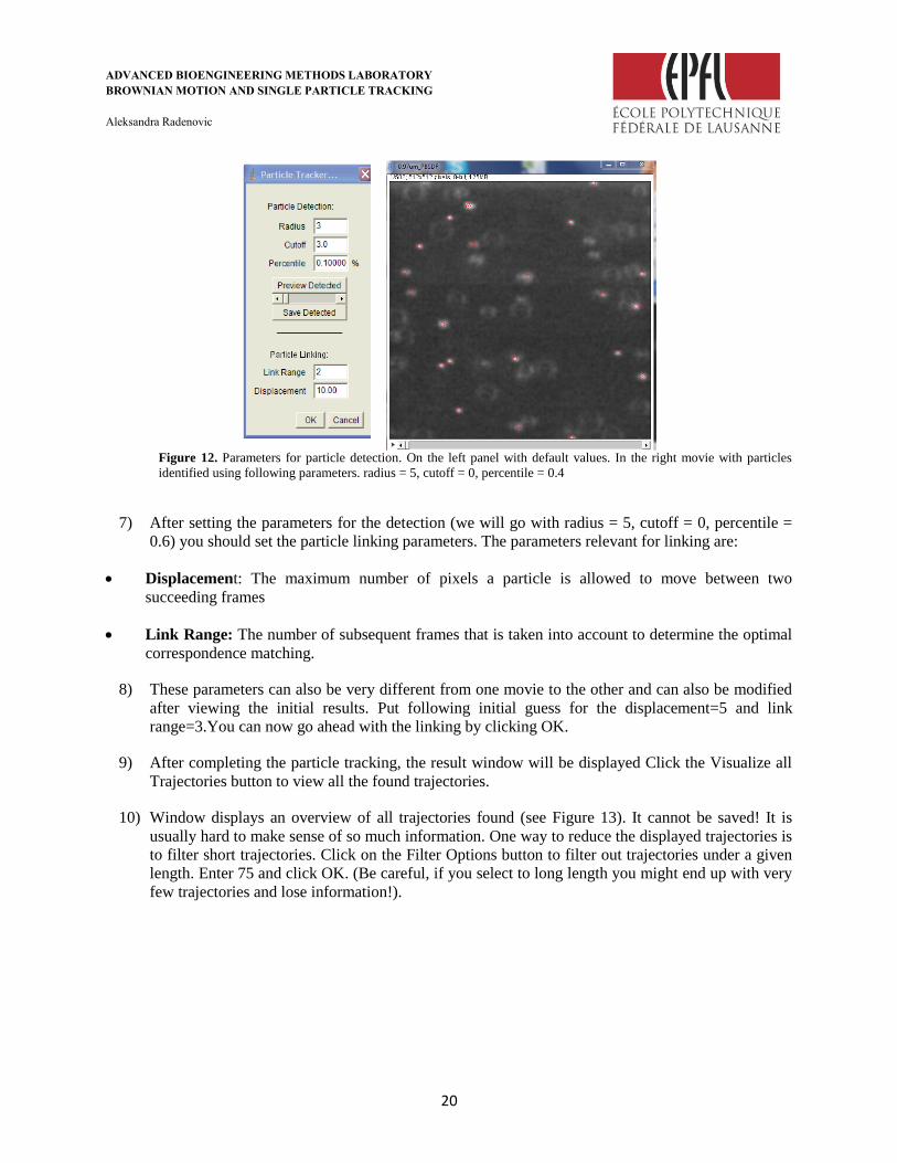
Figure 12 Parameters for particle detection On the left panel with default values In the right movie with particles
identified using following parameters radius = 5 cutoff = 0 percentile = 04
7) After setting the parameters for the detection (we will go with radius = 5 cutoff = 0 percentile =
06) you should set the particle linking parameters The parameters relevant for linking are
Displacement The maximum number of pixels a particle is allowed to move between two
succeeding frames
Link Range The number of subsequent frames that is taken into account to determine the optimal
correspondence matching
8) These parameters can also be very different from one movie to the other and can also be modified
after viewing the initial results Put following initial guess for the displacement=5 and link
range=3You can now go ahead with the linking by clicking OK
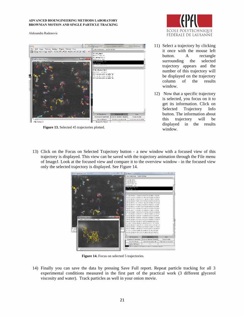
9) After completing the particle tracking the result window will be displayed Click the Visualize all
Trajectories button to view all the found trajectories
10) Window displays an overview of all trajectories found (see Figure 13) It cannot be saved It is
usually hard to make sense of so much information One way to reduce the displayed trajectories is
to filter short trajectories Click on the Filter Options button to filter out trajectories under a given
length Enter 75 and click OK (Be careful if you select to long length you might end up with very
few trajectories and lose information)
ADVANCED BIOENGINEERING METHODS LABORATORY
BROWNIAN MOTION AND SINGLE PARTICLE TRACKING
Aleksandra Radenovic
21
11) Select a trajectory by clicking
it once with the mouse left
button A rectangle
surrounding the selected
trajectory appears and the
number of this trajectory will
be displayed on the trajectory
column of the results
window
12) Now that a specific trajectory
is selected you focus on it to
get its information Click on
Selected Trajectory Info
button The information about
this trajectory will be
displayed in the results
window
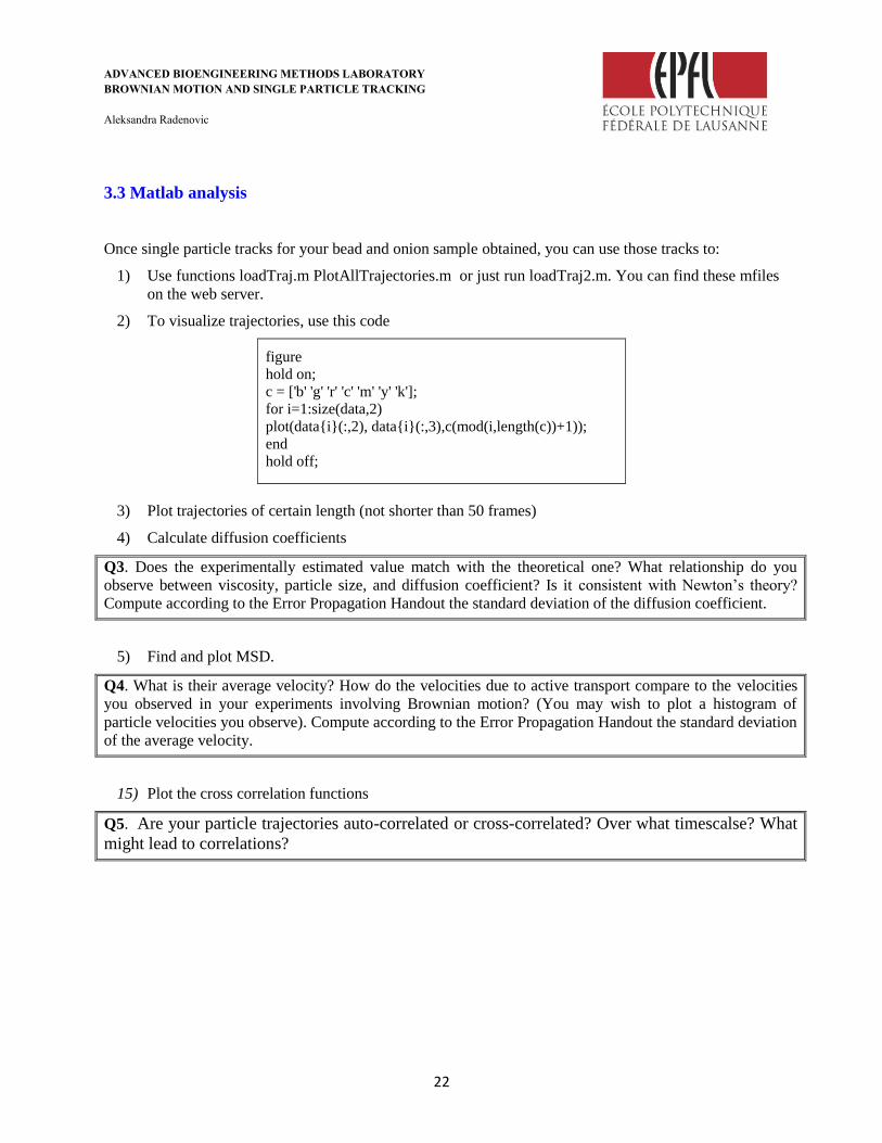
13) Click on the Focus on Selected Trajectory button - a new window with a focused view of this
trajectory is displayed This view can be saved with the trajectory animation through the File menu
of ImageJ Look at the focused view and compare it to the overview window - in the focused view
only the selected trajectory is displayed See Figure 14
Figure 14 Focus on selected 5 trajectories
14) Finally you can save the data by pressing Save Full report Repeat particle tracking for all 3
experimental conditions measured in the first part of the practical work (3 different glycerol
viscosity and water) Track particles as well in your onion movie
Figure 13 Selected 45 trajectories plotted
ADVANCED BIOENGINEERING METHODS LABORATORY
BROWNIAN MOTION AND SINGLE PARTICLE TRACKING
Aleksandra Radenovic
22
33 Matlab analysis
Once single particle tracks for your bead and onion sample obtained you can use those tracks to
1) Use functions loadTrajm PlotAllTrajectoriesm or just run loadTraj2m You can find these mfiles
on the web server
2) To visualize trajectories use this code
figure
hold on
c = [b g r c m y k]
for i=1size(data2)
plot(datai(2) datai(3)c(mod(ilength(c))+1))
end
hold off
3) Plot trajectories of certain length (not shorter than 50 frames)
4) Calculate diffusion coefficients
Q3 Does the experimentally estimated value match with the theoretical one What relationship do you
observe between viscosity particle size and diffusion coefficient Is it consistent with Newtonrsquos theory
Compute according to the Error Propagation Handout the standard deviation of the diffusion coefficient
5) Find and plot MSD
Q4 What is their average velocity How do the velocities due to active transport compare to the velocities
you observed in your experiments involving Brownian motion (You may wish to plot a histogram of
particle velocities you observe) Compute according to the Error Propagation Handout the standard deviation
of the average velocity
15) Plot the cross correlation functions
Q5 Are your particle trajectories auto-correlated or cross-correlated Over what timescalse What
might lead to correlations
ADVANCED BIOENGINEERING METHODS LABORATORY
BROWNIAN MOTION AND SINGLE PARTICLE TRACKING
Aleksandra Radenovic
23
34 Questions
Q6 What is a Newtonian fluid
Q7 Are we really in the inertia-less regime Why or why not
Q8 What would happen if your particles interacted through some potential
Q9 What is meant by viscous coupling Is this something you had to take into account
Q10 What is the amount of work needed to transport a vesicle from the perimeter of the cell to the center
(You can calculate this quantity based on Stokes Law using the particle size and viscosity of the cytosol that
you have already determined)
Q11 Knowing that hydrolysis of an ATP to ADP release 305kJmol compare this quantity to the amount of
work needed to transport a vesicle from the perimeter of the cell to the center
Q12 Calculate the minimum number of myosin motors required to transport a vesicle from the perimeter of
the cell to its center (Each power stroke consumes the energy involved in converting a single molecule of
ATP to ADP remember to correct for the efficiency of the myosin motors (about 018-030)
4 REFERENCES
1 Einstein A Uumlber die von der molekularkinetischen Theorie der Waumlrme geforderte Bewegung von in
ruhenden Fluumlssigkeiten suspendierten Teilchen Ann Phys 17 (1905)
2 Einstein A Theoretische Bemerkungen Uumlber die Brownsche Bewegung Zeitschrift fuumlr Elektrochemie und
angewandte physikalische Chemie 13 41-42 doi101002bbpc19070130602 (1907)
3 Perrin J The Brownian rotational motion Physikalische Zeitschrift 11 470-471 (1910)
4 Perrin J Brownian movement and molecular science Physikalische Zeitschrift 11 461-470 (1910)
5 Perrin J Brownian motion and molecular reality Ann Chim Phys 18 5-114 (1909)
6 Sbalzarini I F amp Koumoutsakos P Feature point tracking and trajectory analysis for video imaging in
cell biology J Struct Biol 151 182-195 doiS1047-8477(05)00126-7 [pii]
101016jjsb200506002 (2005)
Page 2
ADVANCED BIOENGINEERING METHODS LABORATORY
BROWNIAN MOTION AND SINGLE PARTICLE TRACKING
Aleksandra Radenovic
2
TABLE OF CONTENTS
1 Theory 3
11 What is Brownian motion 3
12 Calculation of the Mean Square Displacement 4
13 Intracellular Transport 6
2 Practical work 10
21 Material requirements 10
22 Calibration and Testing 10
23 Viscous suspensions preparation 11
24 Polystyrene suspensions preparation 11
25 Polystyrene suspensions preparation 11
26 Slide loading 12
27 View the slide in transmitted light 13
28 Set-up darkfield illumination 13
29 Viewing Tracking Particles in Viscous Suspensions 13
210 Making an onion slide 15
211 Making observations 16
3 Data analysis 17
31 Calibration 17
32 Particle Tracking 17
33 Matlab analysis 22
34 Questions 23
4 References 23
ADVANCED BIOENGINEERING METHODS LABORATORY
BROWNIAN MOTION AND SINGLE PARTICLE TRACKING
Aleksandra Radenovic
3
Please find the exercise on Brownian motion simulation on the web
site and please do it at home before the practical session
1 THEORY
11 What is Brownian motion
Although it was Jan Ingenhousz who made the first known documented observations of fluctuating
movements of carbon dust particles in alcohol in 1765 the discovery of Brownian motion is credited to
Robert Brown due to his observations of pollen in water in 1827 Also because the previous description
by Ingenhousz was not well known the chaotic movement was for a long time considered to be a
property of living or at least organic matter Brownian motion is stochastic movements of small particles
suspended in a solution The molecules (for example water molecules) constituting the fluid constantly hit
the immersed objects which results in chaotic and non-directed movements These movements can be
measured by the mean square displacement 2
r and the lag time t and is characterized by the
diffusion coefficient D which is a measure of the speed of diffusion For three-dimensional brownian
motions these terms can be put into an equation as follows
2
6r D t (01)
This is only true for isotropic and unrestricted translational diffusion Brownian motion is actually
observed for many different dynamical phenomena Here we concentrate on isotropic translational
displacements (random walk) but brownian motion can be also of rotational undulating etc nature
Translational diffusion or random walk in three dimensions can mathematically be described by a
differential equation
( )
( )r
D rt
(02)
Where ( )r is the particle location distribution and ∆ is the Laplace-Operator which is a second order
differential operator
In 1905 Einstein published a paper that predicted a relationship between the mean squared magnitude of
Brownian excursions and the size of molecules 1-2
Now all that remained was to do the experiment Jean
Perrin 3-5
won the Nobel Prize in 1926 for his work confirming Einsteins hypothesis Perrins
experimental confirmation of Einsteins equation was an important piece of evidence to help settle a
debate about the nature of mater that had begun nearly 2000 years earlier in the time of Democritus and
Anaxagoras Since then a thorough understanding of Brownian motion has become essential for diverse
fields are ranging from polymer physics to biophysics aerodynamics to statistical mechanics and even
stock option pricing
Albert Einstein has calculated the diffusion coefficient to for a spherical particle
3
Bk TD
d
(03)
ADVANCED BIOENGINEERING METHODS LABORATORY
BROWNIAN MOTION AND SINGLE PARTICLE TRACKING
Aleksandra Radenovic
4
where kB is the Boltzmann constant T the temperature η the viscosity of the medium and d the diameter
of the diffusing particle The dimension of the diffusion coefficient is m2s The given relation between
diffusion coefficient temperature viscosity and particle size is only true for isotropic non-hindered
diffusion of a spherical particle The diffusion coefficient therefore gives us information about the
temperature and viscosity of the system and size and shape of the diffusing particle
For two and one dimensions the time dependence of mean square displacements for isotropic diffusion
differs only in the numerical factor
2
2
dim 4
dim 2
two r D t
one x D t
(04)
The diffusion coefficient does not depend on the dimensions in which the diffusion takes place
Hindered or restricted diffusion is for example the case where the particle has to diffuse in a porous or
structured environment as in cells Anisotropic diffusion takes place in cases when the particle itself has
an asymmetric shape Then the diffusion coefficient is no simple scalar like in eq03 anymore but
becomes a complex tensor
12 Calculation of the Mean Square Displacement
In this introduction we want to limit ourselves to a movement in two dimensions Consider a trace of
arbitrary movements (random walk) of a particle as depicted in Figure 1a) The mean square displacement
can be then calculated as follows For each time point separated by a fixed lag time t one obtains a
position xi and yi A displacement is then calculated as
1 1 2 1 1 2 1
1 1 2 1 1 2 1
1 1
1 1
( ) ( ) ( )
( ) ( ) ( )
( ) ( ) ( )
( ) ( ) ( )
i i i i i i i
i i i i i i i
x x t x x t t x t x x
y y t y y t t y t y y
x x t x x t t x t x x
y y t x y t t y t y y
(05)
The t in brackets shall indicate that this step takes place during a time period of a single lag time t
The square displacement 2
r is then the sum of the displacements in respect of the different
dimensions
2 2 2
1 1 1r t x t y t (06)
ADVANCED BIOENGINEERING METHODS LABORATORY
BROWNIAN MOTION AND SINGLE PARTICLE TRACKING
Aleksandra Radenovic
5
Figure 1 a) Random walk in 2D intermediate positions and traces of a diffusing particle Continuous lines indicate the
displacement corresponding to single steps dotted lines to double step during two time intervals b) Squared displacements can
be plotted according to the time intervals Note that for longer steps the number of data points becomes less c) Data points
corresponding to one time interval merge into on average value Fitting should give a straight line for unrestricted and isotropic
diffusion
Q1 Note that the error bar becomes larger for larger steps Why
The displacement and the square displacement can be calculated for every step of the same trace
corresponding to the same step size of stepping time (step during the time length t )
2 2 2
2 2
2 2 2
3 3 3
2 2 2
2
i i i
r t x t y t
r t x t y t
r t x t y t
(07)
The mean square displacement is obtained as an average of all steps corresponding to a single lag time
t
2 2 2 2 2
1 2 1
1
1 1( ) ( ) ( ) ( ) ( )
n
i
i
r t r t r t r t r tn n
(08)
The same procedure applies to double step during a time length of 2 t
Q2 Please provide step by step calculation for 2 t and 3 t
Now the mean square displacement (MSD) can be plotted to its corresponding step time interval which
gives characteristic curves If the analyzed diffusion is of isotropic nature then one would expect a linear
correlation In this case the slope of the line corresponds to the diffusion coefficient multiplied with its
factor (normally 2 4 or 6) Diffusion or random walk can be hindered or restricted which changes the
characteristic form of the MSD plots In the case of diffusion restricted to a confined space the MSD
ADVANCED BIOENGINEERING METHODS LABORATORY
BROWNIAN MOTION AND SINGLE PARTICLE TRACKING
Aleksandra Radenovic
6
naturally does not exceed the diameter of this space as shown in Figure 2 In biological matter one often
finds a combination of both
Figure 2 Different types of random walk and their corresponding MSD plot From left to right Isotropic random walk confined
random walk and partially confined random walk (hopping)
In the first part of this lab you will replicate Perrins work with modern equipment You will track the
motion of synthetic beads suspended in liquids of various viscosities on a research-grade inverted
microscope A CCD camera will transfer images of the beads to a computer for automated particle
tracking and analysis You will explore use of algorithms to improve the identification and tracking of
particles and analyze the effects of particle size viscosity of the solution and molecular weight of the
dissolved solute on the motion of the beads One of the aims of this lab is to directly reproduce the
experiments of J Perrin that led to his Nobel Prize He used latex spheres and we will use polystyrene
spheres otherwise the experiments will be identical In addition to reproducing Perrins results you will
probe further by looking at the effect of varying solvent molecule size
Techniques developed in this lab include bright-fielddark-field microscopy pipetting image data
acquisition theory and software design for image filtering and particle tracking and data analysis in
ImageJ Matlab or Excel Previous programming experience is not required
13 Intracellular Transport
The second part of this experiment consists of observing the motion of particles inside a living cell
Cells transport nutrient waste information etc in membrane-bound vesicles which are visible under a
light microscope An old-fashioned view of a cell was that it is a bag of water containing various
enzymes in which matter is transported passively by diffusion Though diffusion is an important
mechanism it is too slow and random for long distance transport and directing materials where they are
most needed especially in larger cells It is now understood that cells have highly developed and intricate
mechanisms for directed transport of materials
ADVANCED BIOENGINEERING METHODS LABORATORY
BROWNIAN MOTION AND SINGLE PARTICLE TRACKING
Aleksandra Radenovic
7
a b
c
Figure 3 a) The eukaryotic cytoskeleton Actin filaments are shown in red microtubules in green and the nuclei are in blue b)
Cartoon of myosin motors pulling organelles along an actin filament c) Binding of kinesin motor to microtubule
Most motions within and of cells involve two components a cytoskeletal fiber that serves as a track and
a motor protein that does the work (Figure3 a and b) The motor molecule uses energy from the
hydrolysis of one ATP molecule to bind to the fiber bend to pull itself along the fiber and release all of
which constitutes one step For an animation of this stepping process see this movie animation from the
Vale lab web site at UC San Francisco One can divide cellular motility mechanisms into two classes
based on the cytoskeletal fibers involved Microtubule-based mechanisms involve dynein or kinesin
motors pulling on microtubules made of the protein tubulin Actin-based mechanisms involve myosin
motors pulling on actin fibers also called microfibers
Virtually all cell types exhibit directed intracellular transport but some cell types are particularly
suitable for transport studies Fish-scale pigment cells work well since a large fraction of the cargoes that
are transported are pigmented and thus easy to observe ndash the disadvantage is that you would need to bring
a living fish into lab as a source of these cells For convenience we will use epidermal cells from onion
bulbs that you can easily acquire in a grocery store (Coop or Migros) With some care a single layer of
cells can be peeled off from an inner section of the onion bulb and mounted flat on a slide
ADVANCED BIOENGINEERING METHODS LABORATORY
BROWNIAN MOTION AND SINGLE PARTICLE TRACKING
Aleksandra Radenovic
8
a b
Figure 4 a) Onion cells in bright-field illumination Round object in each cell is the nucleus b) Vesicles in the cytoplasm of a
plant cell as seen in dark-field
In this experiment we will be viewing the movement of vesicles within the cytoplasm of onion
epidermal cells shown above as they appear in bright-field and dark-field microscopy Figure 4 a and b
The layers you see in an onion bulb develop into leaves when it sprouts Both sides of the leaf are covered
with an epidermis consisting of brick-shaped cells each with a cell wall and cell membrane on the
outside Most of the interior of the cell is filled with a clear fluid vacuole that functions in storage and in
maintenance of hydrostatic pressure essential to the stiffness of the plant (the difference between crisp
lettuce and wilted lettuce) The cytoplasm containing all of the other cell contents occurs in a thin layer
between the cell membrane and the vacuole and in thin extensions through the vacuole called
transvacuolar strands It is within the cytoplasm that you will be observing directed transport of vesicles
by an actin-based mechanism These vesicles are spherical or rod-shaped organelles such as
mitochondria spherosomes and peroxisomes ranging in size from 05 to 3 microns
The diagram of an onion cell (Figure 5) shows the location of the cell wall cytoplasm and vesicles in a
typical cell you will not be able to see much of the endoplasmic reticulum or the vacuole depicted
because of their transparency Under the microscope you will notice the vesicles are located just along
the edges of the cell or near the top and bottom surface if you focus up and down When you see a
narrow band of moving vesicles in the center of the cell it is located in a transvacuolar strand which may
be a handy place to study motion In plant cells vesicles are transported along actin fibers by myosin
motor molecules An actin filament is composed of two intertwined actin chains about 7 nm in diameter
An actin fiber is considered structurally polar having a (+) end and a (-) end and most myosin motors
move only towards the (+) end of the actin fiber In order to reverse the direction of a vesicles motion the
vesicle must grab on to another actin fiber oriented in the opposite direction There are at least eighteen
described classes of myosin of which three myosin VIII XI and XII are found in plant cells Some
myosin motors are processive meaning that they remain bound to an actin fiber as they move step-by-
step along it (analagous to this movie animation of kinesin Other myosins are non-processive releasing
from the actin fiber after each step Myosin II found in muscle cells is non-processive as illustrated in this
video animation In the muscle functional unit there are many myosin motors acting together so there are
always some attached to the actin fiber The myosin XI responsible for transport of plant cell vesicles is
the fastest myosin known and is processive It is not certain how many myosin molecules are attached to
the surface of a vesicle or how many of those are active at one time in pulling the vesicle along an actin
fiber
ADVANCED BIOENGINEERING METHODS LABORATORY
BROWNIAN MOTION AND SINGLE PARTICLE TRACKING
Aleksandra Radenovic
9
In some plant cells and algal cells a large-scale streaming motion of the cytoplasm is observed logically
called cytoplasmic streaming This bulk flow is believed to be caused by myosin motors pulling the
extensive endoplasmic reticulum along actin fibers lining the cell membrane Many other vesicles are
then dragged along with the endoplasmic reticulum Lodish and Berk et al provide a detailed explanation
of this process and a video of cytoplasmic streaming in the pond weed Elodea can be viewed here
In your observations of vesicles in onion epidermal cells you should distinguish between the random
Brownian motion of vesicles that are unattached (or at least not actively moving along) actin filaments
the directed transport of vesicles by attached myosin motors and possibly (though we are not sure this
really happens in onions) bulk flow of vesicles in cytoplasmic streaming
Figure 5 A 3D cross-section model of an onion
epidermal cell showing actin filaments and vesicles in
the narrow bands of cytoplasm within the cell
ADVANCED BIOENGINEERING METHODS LABORATORY
BROWNIAN MOTION AND SINGLE PARTICLE TRACKING
Aleksandra Radenovic
10
2 PRACTICAL WORK
21 Material requirements
Handling Safety glasses gloves tweezers pipettes spoons razor blades scalpels
Machines IX 71 microscope dark field bright field Pipettor Finpette 10-100μL
Products Synthetic beads from Bangs Laboratories httpwwwbangslabscom (1041μm)
Solvents Glycerol PBS water
Please read the microscopy part as well as the Koehlerdark field illumination part of
the master handout BEFORE using the microscopy
22 Calibration and Testing (done by TA beforehand)
Before taking data in your first investigation you must calibrate the microscope and learn the
experimental techniques involving pipetting microscopy and data-taking Your first slide preparation of
10μm beads will be used to determine the conversion from pixels in the image to μm on the actual
specimen This calibration must be done separately for the microscopes 20x objective lens and 40x
objective lens For testing purposes you will make a slide of 1μm beads in water set up dark-field
illumination on the microscope and experiment with settings of the lighting focus and particle tracker
software to successfully track beads and save data on particle motion Setting up bright-field Kohler
illumination and dark-field illumination requires careful alignment and some practice but this will pay off
later in the quality of your images and data
23 Viscous suspensions preparation
A solution will consist of three parts PBS buffer which makes up most of the solution a solute glycerol
to provide the viscosity and the beads which we will then observe PBS buffer together with glycerol and
beads solution is located in the 4 degC in the fridge and are also clearly marked Note that the glycerol is
extremely sticky (ie viscous) and will not be measured precisely using the pipette as it will stick to both
the inside and outside of the filter tip To measure glycerol it is best to use the scale located at the lab
station Note (11 ratio water glycerol (labeled 50 glycerol by weight) 12 (labeled 75 glycerol by
weight) are also located in the 4 degC fridge
Use the table below to compute the required dilution of the solvent The stock Glycerol is a thick liquid
with gt99 purity It will require some care to measure the pure glycerol accurately since it tends to stick
to the sides of the pipette tip For this reason weighing the glycerol before adding the water is probably a
better technique than adding the glycerol to the water You may either use these values or interpolate
between them
PLEASE do ONLY 3 different viscosities pure water and the other two marked in red
ADVANCED BIOENGINEERING METHODS LABORATORY
BROWNIAN MOTION AND SINGLE PARTICLE TRACKING
Aleksandra Radenovic
11
Glycerol Viscosity versus Concentration
Viscosity (cP) Glycerol to Water Ratio (by weight)
166 1882
25 322678
465 442558
132 645355
Note 1 cP = 1 mPamiddots = 0001 Pamiddots
1) Take out a new plastic vial to contain the viscous solution
2) Turn on the balance
3) Place vial on balance and ensure all of the doors on the enclosure are shut
4) ZeroTare the balance by pressing the 0T button to cancel out the weight of the vial
5) Place a moderate amount of solute into vial
6) Weigh the amount of glycerol using the balance
7) Calculate how much water is needed to obtain the desired viscosity using the table above
8) Add the appropriate amount of water to the vial by pippeting
24 Polystyrene suspensions preparation
Beads are located (and should be kept) in the refrigerator Each of the vials is clearly marked with the
size of bead that it contains (Note The sizes reported on the vials are mean particle diameter not radius)
These vials are often extremely concentrated and you may wish to create your own diluted solution to
work with We have created 125 dilutions already
Note that the densities vary to a small extent between the different size particles For this reason the
following procedure may need to be adjusted slightly for each of the different particle sizes
1) Remove a bead vial of the desired size from refrigerator shake it vigorously to ensure it is mixed
uniformly
2) Using a NEW filter tip extract 20μL from the vial containing (125 bead dilution) and deposit
into a new plastic vial
3) Use the large volume micropipette to add 80μL of desired viscous solution to the same vial
4) Cap vial using a plastic vial top and shake it vigorously to ensure it is mixed uniformly
5) Repeat this process with each experimental condition selected
25 Floating bead slide preparation
Now that we have a proper vial of viscous bead solution made up we need to transfer a sample of it onto
a slide so that we can observe the beads behavior
ADVANCED BIOENGINEERING METHODS LABORATORY
BROWNIAN MOTION AND SINGLE PARTICLE TRACKING
Aleksandra Radenovic
12
1) Take out a slide from its box and carefully rest in a position to minimize dust contamination
2) Place a self-adhesive reinforcement ring onto the center of a new slide This will create a well
for the solution and keep it from drying out See Figure 6
3) Make sure that this label is well pressed down onto the slide to ensure that liquid isnt sucked
out towards the open air Rubbing the edge of another slide over the coverslip provides a good
method of pushing down the well without contaminating the slide with oils from your hands
4) Remove outer adhesive liner
Secure seal
imaging spacers
Beads
glass coverslip
glass slides
buffers
Chamber
Figure 6 Make a beads slides
5) Use the pipette to transfer roughly 30-35μL of your bead solution into the center of the well
6) Cover the slide with one of the small 24 x 60mm coverslips It is important to ensure that air
bubbles do not form beneath the coverslip To prevent this rest one edge of the coverslip on the
slide and then let the other side drop onto the slide (Capillary action will adhere the coverslip to
the slide)
26 Slide loading
1) Move the objective lens away from the microscope stage first before placing the slide onto the
stage
2) The entire carrier arm that holds the HAL 100 illuminator and the condenser tilts backward on a
hinge to facilitate access to the microscope stage Push back gently on the angled metal
nosepiece until the arm comes to a rest
3) Our microscope is an inverted microscope and as such the sample (ie side with the coverslip)
should be positioned such that the coverslip is on the bottom side of the slide This will ensure
that the sample is closest to the objective You will not be able to focus on the sample using the
40x objective if this is not the case
ADVANCED BIOENGINEERING METHODS LABORATORY
BROWNIAN MOTION AND SINGLE PARTICLE TRACKING
Aleksandra Radenovic
13
27 View the slide in transmitted light
In this step you will view your sample under Koumlhler illumination to achieve uniform illumination with
little reflection or glare and minimal sample heating Please find the Koehler illumination protocol in the
master handout
The samples in this lab are difficult to focus on because they have very little contrast If you have trouble
focusing try starting with the 10x objective At higher magnification it is sometimes helpful to focus on
the edge of the slide first to get the setting close
SAFETY (MICROSCOPE MANIPULATION)
Stay away from slower particles for they are close to the edges The eyepieces are designed to be used
while wearing eyeglasses If you do not wear glasses DO NOT get too close to them
28 Set-up darkfield illumination
Now you can set up the dark field illumination Please find the Dark field illumination protocol in the
master handout
1) Select the 20x objective and establish the Koehler illumination
2) Set the dark field illumination
3) Open the field iris all the way
4) Increase the light intensity using the Toggle Switch for Illumination Intensity You will need to
turn the light level up significantly in order to see the small amount of light scattered by the
smaller nanoparticles (even though the PS spheres will be easily visible)
29 Viewing Tracking Particles in Viscous Suspensions
Now that suspensions and sample chambers have been made for each experimental condition and the
microscope has been fully configured we are now ready to take data
1) Use 10μm beads sample to establish the pixel size of your camera (already done by your TA)
2) Turn on the Andor camera
3) Open Andor camera software called Solis
4) Turn the switch on the microscope to send an image to CCD camera
5) Click on the movie camera icon to get a live image from your sample
6) Set up the exposure time to 005s by pressing exposure button (Figure 7)
7) To take pixel calibration image open in the main menu acquisition under setup CCD select
Single and enter the following value exposure time 001-0075s Then under Setup acquisition
open binning to 512-512 pixels you can move binning box to the region around your 10m
bead press Ok and close Acquisition menu
8) Press Record and save image as sif file
ADVANCED BIOENGINEERING METHODS LABORATORY
BROWNIAN MOTION AND SINGLE PARTICLE TRACKING
Aleksandra Radenovic
14
RecordLive Exposure
Figure 7 Andor Solis program for data acquisition Bright field image of 097 m beads
9) Watch out for bulk flow If you see a number of particles moving in one direction they are
likely undergoing bulk flow This could be due to evaporation of liquid from beneath the
coverslip or an air bubble popping or various other conditions If you see bulk flow occuring
your data will be skewed MAKE SURE there is no bulk flow when collecting data
10) Now we are ready to collect movies for your analysis session
11) To setup your movies exposure time t kinetic series length (number of frames in your
movies ) open in the main menu acquisition under setup CCD select Kinetic series enter
following values exposure time 001-01s kinetic series length 200 next under Setup
acquisition open binning to 512-512 pixels you can move binning box to the region containing
the most beads Mark in your notebook the values you entered
12) Press record
13) Save files as sif Collect all necessary data and save them in your folder
14) Repeat this for each experimental condition selected select three viscosities for 097 m beads
15) Once you have finished data collection you will need to convert all sif files in raw files You
can do it file by file or using a batch conversion option in File menu (Main Menu) Make sure
ADVANCED BIOENGINEERING METHODS LABORATORY
BROWNIAN MOTION AND SINGLE PARTICLE TRACKING
Aleksandra Radenovic
15
that you convert it in 16 bit unsigned integer (with range 0-65322) This is format required for
the analysis session
16) For those of you interested in a challenge you can attempt to create a program in C++ or
Matlab to adjust for bulk flow in the slide
17) If you have enough time repeat this experiment for other bead size or add one more viscosity
210 Making an onion slide
We will now try to track particles in a living cell (onion) Before coming to lab obtain an onion from
your favorite produce store If you have forgotten one you can try to find some in 4 degC fridge
1) Use a knife box-cutter razorblade or whatever other cutting tool is provided to cut out an one
inch cube from the onion
2) Take one of the lower layers (activity depends somewhat on depth) and remove the lower
membrane using the forceps this is similar to pulling off a sticker The membrane is a single
layer of cells which makes it particularly clean when viewing through a microscope It should
appear translucent and should be relatively strong Make a slide using this membrane
3) Place a drop of PBS onto a clean slide (dont use water)
4) Place the membrane onto the slide
5) Drop a couple more drops onto the onion and cover with a large 24x60mm cover glass slide
6) Blot excess liquid using a paper towel and mount it onto microscope
Keep in mind that the lifetime of an onion slide is about 30 minutes before it dries out
Onion
glass coverslipglass slidesbuffer membrane
membrane
Figure 8 Make an onion slide
ADVANCED BIOENGINEERING METHODS LABORATORY
BROWNIAN MOTION AND SINGLE PARTICLE TRACKING
Aleksandra Radenovic
16
211Making Observations
First you should spend a little while looking around trying to find some regions of interest Note the
different types of movement and where they tend to occur In particular be sure to investigate regions
around the cell walls around the nucleus and also see if you can find anything happening within the
otherwise empty center of the cell Most of the activity happens on the lower and upper layers of the cell
as the center is occupied with the vacuole which should be devoid of anything except water If you scan
through the depths of a few cells carefully (using the focus knob to move in depth) you should be able to
find isolated actin fibers which make for very clean data-taking Your data analysis will be much easier if
you can isolate the forms of movement within the cell and only take data on one type at a time
If you dont find much activity you could try a different section of onion or another onion altogether
1) Locate a particle that does not appear to be moving around very much (ie look for a particle
undergoing Brownian motion rather than active transport)
2) Take several movies of a number of particles undergoing Brownian motion See Figure 9
3) Take then some movies of particles undergoing active transport within the actin filaments
4) Repeat this for a number of different cells
5) Change the microscope to obtain a transmitted light image of the onion cells
6) Determine the size of the particles by counting the number of pixels each one take up on the
screen as you did with the 10 polystyrene spheres to obtain the pixel to meter conversion
7) Repeat this step as necessary to obtain a statistically acceptable number
Figure 9 Visualized vesicles in onion cells (x20)
ADVANCED BIOENGINEERING METHODS LABORATORY
BROWNIAN MOTION AND SINGLE PARTICLE TRACKING
Aleksandra Radenovic
17
3 DATA ANALYSIS
31 Calibration (already done by your TA)
1) Open in ImageJ your dark filed image of 10m beads taken for bin
size of 512512 pixels
2) Use a line tool in ImageJ toolbox to draw a line across the selected
bead Below the Image J toolbox you will notice xy coordinates of
your line together with the angle and the length of the drawn line
Make sure to draw the line straight across the bead diameter
3) Next open AnalyzeSet Scale from File menu where you enter the
length of 10m bead as known distance It will calculate the pixel
aspect ratio Use these parameters to set a scale on all movies that
you will be processing
Make sure you have used same objective For 40x objective 1m size bead corresponds to 77 pixels
32 Particle Tracking
To obtain single particle trajectories from recorded movies you will need to use Particle Detector and
Tracker which is an ImageJ Plugin for particles detection and tracking from digital videos
The plugin implements the feature point detection and tracking algorithm as described in recent
publication by Sbalzarini et al6 This plugin presents an easy-to-use computationally efficient two-
dimensional feature point-tracking tool for the automated detection and analysis of particle trajectories as
recorded by video imaging in cell biology The tracking process requires no apriori mathematical
modelling of the motion it is self-initializing it discriminates spurious detections and it can handle
temporary occlusion as well as particle appearance and disappearance from the image region The plugin
is well suited for video imaging in cell biology relying on low-intensity fluorescence microscopy It
allows the user to visualize and analyze the detected particles and found trajectories in various ways i)
Preview and save detected particles for separate analysis ii) Global non progressive view on all
trajectories iii) Focused progressive view on individually selected trajectory and iv) Focused progressive
view on trajectories in an area of interest
It also allows the user to find trajectories from uploaded particles position and information text files and
then to plot particles parameters vs time - along a trajectory
1) Before the plugin can be started you must open an image sequence or a movie in ImageJ For
opening your saved movie use the FileImport Raw You should input following parameters as
indicated in Figure 10 (Check your lab notes for number of frames and binning size) Upon file
import you should obtain video sequence of your moving beads
ADVANCED BIOENGINEERING METHODS LABORATORY
BROWNIAN MOTION AND SINGLE PARTICLE TRACKING
Aleksandra Radenovic
18
Figure 10 Import parameters
2) Next you need to improve contrast and adapt your movie so that it can be treated with
ParticleTracker plugin To do so use the ImageType 8 bit option from File menu Next you need
to increase contrast you will do it by using ProcessEnhance Contrast option from File menu It is
safe to select 01saturated pixels under Use Stack Histogram see Figure 11 To filter out noise
use ProcessFilterGaussian blur option from File menu Again safe sigma value to use is
12Befor aoplying this filtering you can preview your movie
Figure 11 Parameters for better movie quality
3) Now that the movie is open and compatible with the plugging you can start the plugin by
selecting ParticleTracker from the Plugins - Particle Detector amp Tracker menu After starting the
plugin a dialog screen is displayed The dialog has two parts ldquoParticle Detectionrdquo and ldquoParticle
Linkingrdquo
Particle Detection This part of the dialog allows you to adjust parameters relevant to the
particle detection (feature point detection) part of the algorithm
ADVANCED BIOENGINEERING METHODS LABORATORY
BROWNIAN MOTION AND SINGLE PARTICLE TRACKING
Aleksandra Radenovic
19
Preview the detected particles in each frame according to the parameters This options offers
assistance in choosing good values for the parameters Save the detected particles according to
the parameters for all frames The parameters relevant for detection are
Radius Approximate radius of the particles in the images in units of pixels The value should
be slightly larger than the visible particle radius but smaller than the smallest inter-particle
separation
Cutoff The score cut-off for the non-particle discrimination
Percentile The percentile (r) that determines which bright pixels are accepted as Particles All
local maxima in the upper rth percentile of the image intensity distribution are considered
candidate Particles Unit percent ()
4) Clicking on the Preview Detected button will circle the detected particles in the current frame
according to the parameters currently set To view the detected particles in other frames use the
slider placed under the Preview Detected button You can adjust the parameters and check how it
affects the detection by clicking again on Preview Detected Depending on the size of your
particles and movie quality you will need to play with parameters
Note that very rarely you detect all particles in the field of view mostly due to the fact that they quickly
go out of focus
5) To start on 097m beads Enter these parameters radius = 5 cutoff = 0 percentile = 04 and click
on preview detected Check the detected particles at the next frames by using the slider in the
dialog menu With radius of 5 they are rightly detected as 2 separate particles If you have any
doubt they are 2 separate particles you can look at the 3rd frame Change the radius to 10 and click
the preview button With this parameter the algorithm wrongfully detects them as one particle
since they are both within the radius of 10 pixels
6) Try other values for the radius parameter Go back to these parameters radius = 5 cutoff = 0
percentile = 04 and click on preview detected It is obvious that there are more real particles in
the image that were not detected Notice that the detected particles are much brighter then the ones
not detected Since the score cut-off is set to zero we can rightfully assume that increasing the
percentile of particle intensity taken will make the algorithm detect more particles (with lower
intensity) The higher the number in the percentile field - the more particles will be detected Try
setting the percentile value to 2 After clicking the preview button you will see that much more
particles are detected in fact too many particles - you will need to find the right balance (for our
dark filed movies between 03-07 )
Remember There is no right and wrong here - it is possible that the original percentile = 01 will be
more suitable even with this film if for example only very high intensity particles are of interest
ADVANCED BIOENGINEERING METHODS LABORATORY
BROWNIAN MOTION AND SINGLE PARTICLE TRACKING
Aleksandra Radenovic
20
Figure 12 Parameters for particle detection On the left panel with default values In the right movie with particles
identified using following parameters radius = 5 cutoff = 0 percentile = 04
7) After setting the parameters for the detection (we will go with radius = 5 cutoff = 0 percentile =
06) you should set the particle linking parameters The parameters relevant for linking are
Displacement The maximum number of pixels a particle is allowed to move between two
succeeding frames
Link Range The number of subsequent frames that is taken into account to determine the optimal
correspondence matching
8) These parameters can also be very different from one movie to the other and can also be modified
after viewing the initial results Put following initial guess for the displacement=5 and link
range=3You can now go ahead with the linking by clicking OK
9) After completing the particle tracking the result window will be displayed Click the Visualize all
Trajectories button to view all the found trajectories
10) Window displays an overview of all trajectories found (see Figure 13) It cannot be saved It is
usually hard to make sense of so much information One way to reduce the displayed trajectories is
to filter short trajectories Click on the Filter Options button to filter out trajectories under a given
length Enter 75 and click OK (Be careful if you select to long length you might end up with very
few trajectories and lose information)
ADVANCED BIOENGINEERING METHODS LABORATORY
BROWNIAN MOTION AND SINGLE PARTICLE TRACKING
Aleksandra Radenovic
21
11) Select a trajectory by clicking
it once with the mouse left
button A rectangle
surrounding the selected
trajectory appears and the
number of this trajectory will
be displayed on the trajectory
column of the results
window
12) Now that a specific trajectory
is selected you focus on it to
get its information Click on
Selected Trajectory Info
button The information about
this trajectory will be
displayed in the results
window
13) Click on the Focus on Selected Trajectory button - a new window with a focused view of this
trajectory is displayed This view can be saved with the trajectory animation through the File menu
of ImageJ Look at the focused view and compare it to the overview window - in the focused view
only the selected trajectory is displayed See Figure 14
Figure 14 Focus on selected 5 trajectories
14) Finally you can save the data by pressing Save Full report Repeat particle tracking for all 3
experimental conditions measured in the first part of the practical work (3 different glycerol
viscosity and water) Track particles as well in your onion movie
Figure 13 Selected 45 trajectories plotted
ADVANCED BIOENGINEERING METHODS LABORATORY
BROWNIAN MOTION AND SINGLE PARTICLE TRACKING
Aleksandra Radenovic
22
33 Matlab analysis
Once single particle tracks for your bead and onion sample obtained you can use those tracks to
1) Use functions loadTrajm PlotAllTrajectoriesm or just run loadTraj2m You can find these mfiles
on the web server
2) To visualize trajectories use this code
figure
hold on
c = [b g r c m y k]
for i=1size(data2)
plot(datai(2) datai(3)c(mod(ilength(c))+1))
end
hold off
3) Plot trajectories of certain length (not shorter than 50 frames)
4) Calculate diffusion coefficients
Q3 Does the experimentally estimated value match with the theoretical one What relationship do you
observe between viscosity particle size and diffusion coefficient Is it consistent with Newtonrsquos theory
Compute according to the Error Propagation Handout the standard deviation of the diffusion coefficient
5) Find and plot MSD
Q4 What is their average velocity How do the velocities due to active transport compare to the velocities
you observed in your experiments involving Brownian motion (You may wish to plot a histogram of
particle velocities you observe) Compute according to the Error Propagation Handout the standard deviation
of the average velocity
15) Plot the cross correlation functions
Q5 Are your particle trajectories auto-correlated or cross-correlated Over what timescalse What
might lead to correlations
ADVANCED BIOENGINEERING METHODS LABORATORY
BROWNIAN MOTION AND SINGLE PARTICLE TRACKING
Aleksandra Radenovic
23
34 Questions
Q6 What is a Newtonian fluid
Q7 Are we really in the inertia-less regime Why or why not
Q8 What would happen if your particles interacted through some potential
Q9 What is meant by viscous coupling Is this something you had to take into account
Q10 What is the amount of work needed to transport a vesicle from the perimeter of the cell to the center
(You can calculate this quantity based on Stokes Law using the particle size and viscosity of the cytosol that
you have already determined)
Q11 Knowing that hydrolysis of an ATP to ADP release 305kJmol compare this quantity to the amount of
work needed to transport a vesicle from the perimeter of the cell to the center
Q12 Calculate the minimum number of myosin motors required to transport a vesicle from the perimeter of
the cell to its center (Each power stroke consumes the energy involved in converting a single molecule of
ATP to ADP remember to correct for the efficiency of the myosin motors (about 018-030)
4 REFERENCES
1 Einstein A Uumlber die von der molekularkinetischen Theorie der Waumlrme geforderte Bewegung von in
ruhenden Fluumlssigkeiten suspendierten Teilchen Ann Phys 17 (1905)
2 Einstein A Theoretische Bemerkungen Uumlber die Brownsche Bewegung Zeitschrift fuumlr Elektrochemie und
angewandte physikalische Chemie 13 41-42 doi101002bbpc19070130602 (1907)
3 Perrin J The Brownian rotational motion Physikalische Zeitschrift 11 470-471 (1910)
4 Perrin J Brownian movement and molecular science Physikalische Zeitschrift 11 461-470 (1910)
5 Perrin J Brownian motion and molecular reality Ann Chim Phys 18 5-114 (1909)
6 Sbalzarini I F amp Koumoutsakos P Feature point tracking and trajectory analysis for video imaging in
cell biology J Struct Biol 151 182-195 doiS1047-8477(05)00126-7 [pii]
101016jjsb200506002 (2005)
Page 3
ADVANCED BIOENGINEERING METHODS LABORATORY
BROWNIAN MOTION AND SINGLE PARTICLE TRACKING
Aleksandra Radenovic
3
Please find the exercise on Brownian motion simulation on the web
site and please do it at home before the practical session
1 THEORY
11 What is Brownian motion
Although it was Jan Ingenhousz who made the first known documented observations of fluctuating
movements of carbon dust particles in alcohol in 1765 the discovery of Brownian motion is credited to
Robert Brown due to his observations of pollen in water in 1827 Also because the previous description
by Ingenhousz was not well known the chaotic movement was for a long time considered to be a
property of living or at least organic matter Brownian motion is stochastic movements of small particles
suspended in a solution The molecules (for example water molecules) constituting the fluid constantly hit
the immersed objects which results in chaotic and non-directed movements These movements can be
measured by the mean square displacement 2
r and the lag time t and is characterized by the
diffusion coefficient D which is a measure of the speed of diffusion For three-dimensional brownian
motions these terms can be put into an equation as follows
2
6r D t (01)
This is only true for isotropic and unrestricted translational diffusion Brownian motion is actually
observed for many different dynamical phenomena Here we concentrate on isotropic translational
displacements (random walk) but brownian motion can be also of rotational undulating etc nature
Translational diffusion or random walk in three dimensions can mathematically be described by a
differential equation
( )
( )r
D rt
(02)
Where ( )r is the particle location distribution and ∆ is the Laplace-Operator which is a second order
differential operator
In 1905 Einstein published a paper that predicted a relationship between the mean squared magnitude of
Brownian excursions and the size of molecules 1-2
Now all that remained was to do the experiment Jean
Perrin 3-5
won the Nobel Prize in 1926 for his work confirming Einsteins hypothesis Perrins
experimental confirmation of Einsteins equation was an important piece of evidence to help settle a
debate about the nature of mater that had begun nearly 2000 years earlier in the time of Democritus and
Anaxagoras Since then a thorough understanding of Brownian motion has become essential for diverse
fields are ranging from polymer physics to biophysics aerodynamics to statistical mechanics and even
stock option pricing
Albert Einstein has calculated the diffusion coefficient to for a spherical particle
3
Bk TD
d
(03)
ADVANCED BIOENGINEERING METHODS LABORATORY
BROWNIAN MOTION AND SINGLE PARTICLE TRACKING
Aleksandra Radenovic
4
where kB is the Boltzmann constant T the temperature η the viscosity of the medium and d the diameter
of the diffusing particle The dimension of the diffusion coefficient is m2s The given relation between
diffusion coefficient temperature viscosity and particle size is only true for isotropic non-hindered
diffusion of a spherical particle The diffusion coefficient therefore gives us information about the
temperature and viscosity of the system and size and shape of the diffusing particle
For two and one dimensions the time dependence of mean square displacements for isotropic diffusion
differs only in the numerical factor
2
2
dim 4
dim 2
two r D t
one x D t
(04)
The diffusion coefficient does not depend on the dimensions in which the diffusion takes place
Hindered or restricted diffusion is for example the case where the particle has to diffuse in a porous or
structured environment as in cells Anisotropic diffusion takes place in cases when the particle itself has
an asymmetric shape Then the diffusion coefficient is no simple scalar like in eq03 anymore but
becomes a complex tensor
12 Calculation of the Mean Square Displacement
In this introduction we want to limit ourselves to a movement in two dimensions Consider a trace of
arbitrary movements (random walk) of a particle as depicted in Figure 1a) The mean square displacement
can be then calculated as follows For each time point separated by a fixed lag time t one obtains a
position xi and yi A displacement is then calculated as
1 1 2 1 1 2 1
1 1 2 1 1 2 1
1 1
1 1
( ) ( ) ( )
( ) ( ) ( )
( ) ( ) ( )
( ) ( ) ( )
i i i i i i i
i i i i i i i
x x t x x t t x t x x
y y t y y t t y t y y
x x t x x t t x t x x
y y t x y t t y t y y
(05)
The t in brackets shall indicate that this step takes place during a time period of a single lag time t
The square displacement 2
r is then the sum of the displacements in respect of the different
dimensions
2 2 2
1 1 1r t x t y t (06)
ADVANCED BIOENGINEERING METHODS LABORATORY
BROWNIAN MOTION AND SINGLE PARTICLE TRACKING
Aleksandra Radenovic
5
Figure 1 a) Random walk in 2D intermediate positions and traces of a diffusing particle Continuous lines indicate the
displacement corresponding to single steps dotted lines to double step during two time intervals b) Squared displacements can
be plotted according to the time intervals Note that for longer steps the number of data points becomes less c) Data points
corresponding to one time interval merge into on average value Fitting should give a straight line for unrestricted and isotropic
diffusion
Q1 Note that the error bar becomes larger for larger steps Why
The displacement and the square displacement can be calculated for every step of the same trace
corresponding to the same step size of stepping time (step during the time length t )
2 2 2
2 2
2 2 2
3 3 3
2 2 2
2
i i i
r t x t y t
r t x t y t
r t x t y t
(07)
The mean square displacement is obtained as an average of all steps corresponding to a single lag time
t
2 2 2 2 2
1 2 1
1
1 1( ) ( ) ( ) ( ) ( )
n
i
i
r t r t r t r t r tn n
(08)
The same procedure applies to double step during a time length of 2 t
Q2 Please provide step by step calculation for 2 t and 3 t
Now the mean square displacement (MSD) can be plotted to its corresponding step time interval which
gives characteristic curves If the analyzed diffusion is of isotropic nature then one would expect a linear
correlation In this case the slope of the line corresponds to the diffusion coefficient multiplied with its
factor (normally 2 4 or 6) Diffusion or random walk can be hindered or restricted which changes the
characteristic form of the MSD plots In the case of diffusion restricted to a confined space the MSD
ADVANCED BIOENGINEERING METHODS LABORATORY
BROWNIAN MOTION AND SINGLE PARTICLE TRACKING
Aleksandra Radenovic
6
naturally does not exceed the diameter of this space as shown in Figure 2 In biological matter one often
finds a combination of both
Figure 2 Different types of random walk and their corresponding MSD plot From left to right Isotropic random walk confined
random walk and partially confined random walk (hopping)
In the first part of this lab you will replicate Perrins work with modern equipment You will track the
motion of synthetic beads suspended in liquids of various viscosities on a research-grade inverted
microscope A CCD camera will transfer images of the beads to a computer for automated particle
tracking and analysis You will explore use of algorithms to improve the identification and tracking of
particles and analyze the effects of particle size viscosity of the solution and molecular weight of the
dissolved solute on the motion of the beads One of the aims of this lab is to directly reproduce the
experiments of J Perrin that led to his Nobel Prize He used latex spheres and we will use polystyrene
spheres otherwise the experiments will be identical In addition to reproducing Perrins results you will
probe further by looking at the effect of varying solvent molecule size
Techniques developed in this lab include bright-fielddark-field microscopy pipetting image data
acquisition theory and software design for image filtering and particle tracking and data analysis in
ImageJ Matlab or Excel Previous programming experience is not required
13 Intracellular Transport
The second part of this experiment consists of observing the motion of particles inside a living cell
Cells transport nutrient waste information etc in membrane-bound vesicles which are visible under a
light microscope An old-fashioned view of a cell was that it is a bag of water containing various
enzymes in which matter is transported passively by diffusion Though diffusion is an important
mechanism it is too slow and random for long distance transport and directing materials where they are
most needed especially in larger cells It is now understood that cells have highly developed and intricate
mechanisms for directed transport of materials
ADVANCED BIOENGINEERING METHODS LABORATORY
BROWNIAN MOTION AND SINGLE PARTICLE TRACKING
Aleksandra Radenovic
7
a b
c
Figure 3 a) The eukaryotic cytoskeleton Actin filaments are shown in red microtubules in green and the nuclei are in blue b)
Cartoon of myosin motors pulling organelles along an actin filament c) Binding of kinesin motor to microtubule
Most motions within and of cells involve two components a cytoskeletal fiber that serves as a track and
a motor protein that does the work (Figure3 a and b) The motor molecule uses energy from the
hydrolysis of one ATP molecule to bind to the fiber bend to pull itself along the fiber and release all of
which constitutes one step For an animation of this stepping process see this movie animation from the
Vale lab web site at UC San Francisco One can divide cellular motility mechanisms into two classes
based on the cytoskeletal fibers involved Microtubule-based mechanisms involve dynein or kinesin
motors pulling on microtubules made of the protein tubulin Actin-based mechanisms involve myosin
motors pulling on actin fibers also called microfibers
Virtually all cell types exhibit directed intracellular transport but some cell types are particularly
suitable for transport studies Fish-scale pigment cells work well since a large fraction of the cargoes that
are transported are pigmented and thus easy to observe ndash the disadvantage is that you would need to bring
a living fish into lab as a source of these cells For convenience we will use epidermal cells from onion
bulbs that you can easily acquire in a grocery store (Coop or Migros) With some care a single layer of
cells can be peeled off from an inner section of the onion bulb and mounted flat on a slide
ADVANCED BIOENGINEERING METHODS LABORATORY
BROWNIAN MOTION AND SINGLE PARTICLE TRACKING
Aleksandra Radenovic
8
a b
Figure 4 a) Onion cells in bright-field illumination Round object in each cell is the nucleus b) Vesicles in the cytoplasm of a
plant cell as seen in dark-field
In this experiment we will be viewing the movement of vesicles within the cytoplasm of onion
epidermal cells shown above as they appear in bright-field and dark-field microscopy Figure 4 a and b
The layers you see in an onion bulb develop into leaves when it sprouts Both sides of the leaf are covered
with an epidermis consisting of brick-shaped cells each with a cell wall and cell membrane on the
outside Most of the interior of the cell is filled with a clear fluid vacuole that functions in storage and in
maintenance of hydrostatic pressure essential to the stiffness of the plant (the difference between crisp
lettuce and wilted lettuce) The cytoplasm containing all of the other cell contents occurs in a thin layer
between the cell membrane and the vacuole and in thin extensions through the vacuole called
transvacuolar strands It is within the cytoplasm that you will be observing directed transport of vesicles
by an actin-based mechanism These vesicles are spherical or rod-shaped organelles such as
mitochondria spherosomes and peroxisomes ranging in size from 05 to 3 microns
The diagram of an onion cell (Figure 5) shows the location of the cell wall cytoplasm and vesicles in a
typical cell you will not be able to see much of the endoplasmic reticulum or the vacuole depicted
because of their transparency Under the microscope you will notice the vesicles are located just along
the edges of the cell or near the top and bottom surface if you focus up and down When you see a
narrow band of moving vesicles in the center of the cell it is located in a transvacuolar strand which may
be a handy place to study motion In plant cells vesicles are transported along actin fibers by myosin
motor molecules An actin filament is composed of two intertwined actin chains about 7 nm in diameter
An actin fiber is considered structurally polar having a (+) end and a (-) end and most myosin motors
move only towards the (+) end of the actin fiber In order to reverse the direction of a vesicles motion the
vesicle must grab on to another actin fiber oriented in the opposite direction There are at least eighteen
described classes of myosin of which three myosin VIII XI and XII are found in plant cells Some
myosin motors are processive meaning that they remain bound to an actin fiber as they move step-by-
step along it (analagous to this movie animation of kinesin Other myosins are non-processive releasing
from the actin fiber after each step Myosin II found in muscle cells is non-processive as illustrated in this
video animation In the muscle functional unit there are many myosin motors acting together so there are
always some attached to the actin fiber The myosin XI responsible for transport of plant cell vesicles is
the fastest myosin known and is processive It is not certain how many myosin molecules are attached to
the surface of a vesicle or how many of those are active at one time in pulling the vesicle along an actin
fiber
ADVANCED BIOENGINEERING METHODS LABORATORY
BROWNIAN MOTION AND SINGLE PARTICLE TRACKING
Aleksandra Radenovic
9
In some plant cells and algal cells a large-scale streaming motion of the cytoplasm is observed logically
called cytoplasmic streaming This bulk flow is believed to be caused by myosin motors pulling the
extensive endoplasmic reticulum along actin fibers lining the cell membrane Many other vesicles are
then dragged along with the endoplasmic reticulum Lodish and Berk et al provide a detailed explanation
of this process and a video of cytoplasmic streaming in the pond weed Elodea can be viewed here
In your observations of vesicles in onion epidermal cells you should distinguish between the random
Brownian motion of vesicles that are unattached (or at least not actively moving along) actin filaments
the directed transport of vesicles by attached myosin motors and possibly (though we are not sure this
really happens in onions) bulk flow of vesicles in cytoplasmic streaming
Figure 5 A 3D cross-section model of an onion
epidermal cell showing actin filaments and vesicles in
the narrow bands of cytoplasm within the cell
ADVANCED BIOENGINEERING METHODS LABORATORY
BROWNIAN MOTION AND SINGLE PARTICLE TRACKING
Aleksandra Radenovic
10
2 PRACTICAL WORK
21 Material requirements
Handling Safety glasses gloves tweezers pipettes spoons razor blades scalpels
Machines IX 71 microscope dark field bright field Pipettor Finpette 10-100μL
Products Synthetic beads from Bangs Laboratories httpwwwbangslabscom (1041μm)
Solvents Glycerol PBS water
Please read the microscopy part as well as the Koehlerdark field illumination part of
the master handout BEFORE using the microscopy
22 Calibration and Testing (done by TA beforehand)
Before taking data in your first investigation you must calibrate the microscope and learn the
experimental techniques involving pipetting microscopy and data-taking Your first slide preparation of
10μm beads will be used to determine the conversion from pixels in the image to μm on the actual
specimen This calibration must be done separately for the microscopes 20x objective lens and 40x
objective lens For testing purposes you will make a slide of 1μm beads in water set up dark-field
illumination on the microscope and experiment with settings of the lighting focus and particle tracker
software to successfully track beads and save data on particle motion Setting up bright-field Kohler
illumination and dark-field illumination requires careful alignment and some practice but this will pay off
later in the quality of your images and data
23 Viscous suspensions preparation
A solution will consist of three parts PBS buffer which makes up most of the solution a solute glycerol
to provide the viscosity and the beads which we will then observe PBS buffer together with glycerol and
beads solution is located in the 4 degC in the fridge and are also clearly marked Note that the glycerol is
extremely sticky (ie viscous) and will not be measured precisely using the pipette as it will stick to both
the inside and outside of the filter tip To measure glycerol it is best to use the scale located at the lab
station Note (11 ratio water glycerol (labeled 50 glycerol by weight) 12 (labeled 75 glycerol by
weight) are also located in the 4 degC fridge
Use the table below to compute the required dilution of the solvent The stock Glycerol is a thick liquid
with gt99 purity It will require some care to measure the pure glycerol accurately since it tends to stick
to the sides of the pipette tip For this reason weighing the glycerol before adding the water is probably a
better technique than adding the glycerol to the water You may either use these values or interpolate
between them
PLEASE do ONLY 3 different viscosities pure water and the other two marked in red
ADVANCED BIOENGINEERING METHODS LABORATORY
BROWNIAN MOTION AND SINGLE PARTICLE TRACKING
Aleksandra Radenovic
11
Glycerol Viscosity versus Concentration
Viscosity (cP) Glycerol to Water Ratio (by weight)
166 1882
25 322678
465 442558
132 645355
Note 1 cP = 1 mPamiddots = 0001 Pamiddots
1) Take out a new plastic vial to contain the viscous solution
2) Turn on the balance
3) Place vial on balance and ensure all of the doors on the enclosure are shut
4) ZeroTare the balance by pressing the 0T button to cancel out the weight of the vial
5) Place a moderate amount of solute into vial
6) Weigh the amount of glycerol using the balance
7) Calculate how much water is needed to obtain the desired viscosity using the table above
8) Add the appropriate amount of water to the vial by pippeting
24 Polystyrene suspensions preparation
Beads are located (and should be kept) in the refrigerator Each of the vials is clearly marked with the
size of bead that it contains (Note The sizes reported on the vials are mean particle diameter not radius)
These vials are often extremely concentrated and you may wish to create your own diluted solution to
work with We have created 125 dilutions already
Note that the densities vary to a small extent between the different size particles For this reason the
following procedure may need to be adjusted slightly for each of the different particle sizes
1) Remove a bead vial of the desired size from refrigerator shake it vigorously to ensure it is mixed
uniformly
2) Using a NEW filter tip extract 20μL from the vial containing (125 bead dilution) and deposit
into a new plastic vial
3) Use the large volume micropipette to add 80μL of desired viscous solution to the same vial
4) Cap vial using a plastic vial top and shake it vigorously to ensure it is mixed uniformly
5) Repeat this process with each experimental condition selected
25 Floating bead slide preparation
Now that we have a proper vial of viscous bead solution made up we need to transfer a sample of it onto
a slide so that we can observe the beads behavior
ADVANCED BIOENGINEERING METHODS LABORATORY
BROWNIAN MOTION AND SINGLE PARTICLE TRACKING
Aleksandra Radenovic
12
1) Take out a slide from its box and carefully rest in a position to minimize dust contamination
2) Place a self-adhesive reinforcement ring onto the center of a new slide This will create a well
for the solution and keep it from drying out See Figure 6
3) Make sure that this label is well pressed down onto the slide to ensure that liquid isnt sucked
out towards the open air Rubbing the edge of another slide over the coverslip provides a good
method of pushing down the well without contaminating the slide with oils from your hands
4) Remove outer adhesive liner
Secure seal
imaging spacers
Beads
glass coverslip
glass slides
buffers
Chamber
Figure 6 Make a beads slides
5) Use the pipette to transfer roughly 30-35μL of your bead solution into the center of the well
6) Cover the slide with one of the small 24 x 60mm coverslips It is important to ensure that air
bubbles do not form beneath the coverslip To prevent this rest one edge of the coverslip on the
slide and then let the other side drop onto the slide (Capillary action will adhere the coverslip to
the slide)
26 Slide loading
1) Move the objective lens away from the microscope stage first before placing the slide onto the
stage
2) The entire carrier arm that holds the HAL 100 illuminator and the condenser tilts backward on a
hinge to facilitate access to the microscope stage Push back gently on the angled metal
nosepiece until the arm comes to a rest
3) Our microscope is an inverted microscope and as such the sample (ie side with the coverslip)
should be positioned such that the coverslip is on the bottom side of the slide This will ensure
that the sample is closest to the objective You will not be able to focus on the sample using the
40x objective if this is not the case
ADVANCED BIOENGINEERING METHODS LABORATORY
BROWNIAN MOTION AND SINGLE PARTICLE TRACKING
Aleksandra Radenovic
13
27 View the slide in transmitted light
In this step you will view your sample under Koumlhler illumination to achieve uniform illumination with
little reflection or glare and minimal sample heating Please find the Koehler illumination protocol in the
master handout
The samples in this lab are difficult to focus on because they have very little contrast If you have trouble
focusing try starting with the 10x objective At higher magnification it is sometimes helpful to focus on
the edge of the slide first to get the setting close
SAFETY (MICROSCOPE MANIPULATION)
Stay away from slower particles for they are close to the edges The eyepieces are designed to be used
while wearing eyeglasses If you do not wear glasses DO NOT get too close to them
28 Set-up darkfield illumination
Now you can set up the dark field illumination Please find the Dark field illumination protocol in the
master handout
1) Select the 20x objective and establish the Koehler illumination
2) Set the dark field illumination
3) Open the field iris all the way
4) Increase the light intensity using the Toggle Switch for Illumination Intensity You will need to
turn the light level up significantly in order to see the small amount of light scattered by the
smaller nanoparticles (even though the PS spheres will be easily visible)
29 Viewing Tracking Particles in Viscous Suspensions
Now that suspensions and sample chambers have been made for each experimental condition and the
microscope has been fully configured we are now ready to take data
1) Use 10μm beads sample to establish the pixel size of your camera (already done by your TA)
2) Turn on the Andor camera
3) Open Andor camera software called Solis
4) Turn the switch on the microscope to send an image to CCD camera
5) Click on the movie camera icon to get a live image from your sample
6) Set up the exposure time to 005s by pressing exposure button (Figure 7)
7) To take pixel calibration image open in the main menu acquisition under setup CCD select
Single and enter the following value exposure time 001-0075s Then under Setup acquisition
open binning to 512-512 pixels you can move binning box to the region around your 10m
bead press Ok and close Acquisition menu
8) Press Record and save image as sif file
ADVANCED BIOENGINEERING METHODS LABORATORY
BROWNIAN MOTION AND SINGLE PARTICLE TRACKING
Aleksandra Radenovic
14
RecordLive Exposure
Figure 7 Andor Solis program for data acquisition Bright field image of 097 m beads
9) Watch out for bulk flow If you see a number of particles moving in one direction they are
likely undergoing bulk flow This could be due to evaporation of liquid from beneath the
coverslip or an air bubble popping or various other conditions If you see bulk flow occuring
your data will be skewed MAKE SURE there is no bulk flow when collecting data
10) Now we are ready to collect movies for your analysis session
11) To setup your movies exposure time t kinetic series length (number of frames in your
movies ) open in the main menu acquisition under setup CCD select Kinetic series enter
following values exposure time 001-01s kinetic series length 200 next under Setup
acquisition open binning to 512-512 pixels you can move binning box to the region containing
the most beads Mark in your notebook the values you entered
12) Press record
13) Save files as sif Collect all necessary data and save them in your folder
14) Repeat this for each experimental condition selected select three viscosities for 097 m beads
15) Once you have finished data collection you will need to convert all sif files in raw files You
can do it file by file or using a batch conversion option in File menu (Main Menu) Make sure
ADVANCED BIOENGINEERING METHODS LABORATORY
BROWNIAN MOTION AND SINGLE PARTICLE TRACKING
Aleksandra Radenovic
15
that you convert it in 16 bit unsigned integer (with range 0-65322) This is format required for
the analysis session
16) For those of you interested in a challenge you can attempt to create a program in C++ or
Matlab to adjust for bulk flow in the slide
17) If you have enough time repeat this experiment for other bead size or add one more viscosity
210 Making an onion slide
We will now try to track particles in a living cell (onion) Before coming to lab obtain an onion from
your favorite produce store If you have forgotten one you can try to find some in 4 degC fridge
1) Use a knife box-cutter razorblade or whatever other cutting tool is provided to cut out an one
inch cube from the onion
2) Take one of the lower layers (activity depends somewhat on depth) and remove the lower
membrane using the forceps this is similar to pulling off a sticker The membrane is a single
layer of cells which makes it particularly clean when viewing through a microscope It should
appear translucent and should be relatively strong Make a slide using this membrane
3) Place a drop of PBS onto a clean slide (dont use water)
4) Place the membrane onto the slide
5) Drop a couple more drops onto the onion and cover with a large 24x60mm cover glass slide
6) Blot excess liquid using a paper towel and mount it onto microscope
Keep in mind that the lifetime of an onion slide is about 30 minutes before it dries out
Onion
glass coverslipglass slidesbuffer membrane
membrane
Figure 8 Make an onion slide
ADVANCED BIOENGINEERING METHODS LABORATORY
BROWNIAN MOTION AND SINGLE PARTICLE TRACKING
Aleksandra Radenovic
16
211Making Observations
First you should spend a little while looking around trying to find some regions of interest Note the
different types of movement and where they tend to occur In particular be sure to investigate regions
around the cell walls around the nucleus and also see if you can find anything happening within the
otherwise empty center of the cell Most of the activity happens on the lower and upper layers of the cell
as the center is occupied with the vacuole which should be devoid of anything except water If you scan
through the depths of a few cells carefully (using the focus knob to move in depth) you should be able to
find isolated actin fibers which make for very clean data-taking Your data analysis will be much easier if
you can isolate the forms of movement within the cell and only take data on one type at a time
If you dont find much activity you could try a different section of onion or another onion altogether
1) Locate a particle that does not appear to be moving around very much (ie look for a particle
undergoing Brownian motion rather than active transport)
2) Take several movies of a number of particles undergoing Brownian motion See Figure 9
3) Take then some movies of particles undergoing active transport within the actin filaments
4) Repeat this for a number of different cells
5) Change the microscope to obtain a transmitted light image of the onion cells
6) Determine the size of the particles by counting the number of pixels each one take up on the
screen as you did with the 10 polystyrene spheres to obtain the pixel to meter conversion
7) Repeat this step as necessary to obtain a statistically acceptable number
Figure 9 Visualized vesicles in onion cells (x20)
ADVANCED BIOENGINEERING METHODS LABORATORY
BROWNIAN MOTION AND SINGLE PARTICLE TRACKING
Aleksandra Radenovic
17
3 DATA ANALYSIS
31 Calibration (already done by your TA)
1) Open in ImageJ your dark filed image of 10m beads taken for bin
size of 512512 pixels
2) Use a line tool in ImageJ toolbox to draw a line across the selected
bead Below the Image J toolbox you will notice xy coordinates of
your line together with the angle and the length of the drawn line
Make sure to draw the line straight across the bead diameter
3) Next open AnalyzeSet Scale from File menu where you enter the
length of 10m bead as known distance It will calculate the pixel
aspect ratio Use these parameters to set a scale on all movies that
you will be processing
Make sure you have used same objective For 40x objective 1m size bead corresponds to 77 pixels
32 Particle Tracking
To obtain single particle trajectories from recorded movies you will need to use Particle Detector and
Tracker which is an ImageJ Plugin for particles detection and tracking from digital videos
The plugin implements the feature point detection and tracking algorithm as described in recent
publication by Sbalzarini et al6 This plugin presents an easy-to-use computationally efficient two-
dimensional feature point-tracking tool for the automated detection and analysis of particle trajectories as
recorded by video imaging in cell biology The tracking process requires no apriori mathematical
modelling of the motion it is self-initializing it discriminates spurious detections and it can handle
temporary occlusion as well as particle appearance and disappearance from the image region The plugin
is well suited for video imaging in cell biology relying on low-intensity fluorescence microscopy It
allows the user to visualize and analyze the detected particles and found trajectories in various ways i)
Preview and save detected particles for separate analysis ii) Global non progressive view on all
trajectories iii) Focused progressive view on individually selected trajectory and iv) Focused progressive
view on trajectories in an area of interest
It also allows the user to find trajectories from uploaded particles position and information text files and
then to plot particles parameters vs time - along a trajectory
1) Before the plugin can be started you must open an image sequence or a movie in ImageJ For
opening your saved movie use the FileImport Raw You should input following parameters as
indicated in Figure 10 (Check your lab notes for number of frames and binning size) Upon file
import you should obtain video sequence of your moving beads
ADVANCED BIOENGINEERING METHODS LABORATORY
BROWNIAN MOTION AND SINGLE PARTICLE TRACKING
Aleksandra Radenovic
18
Figure 10 Import parameters
2) Next you need to improve contrast and adapt your movie so that it can be treated with
ParticleTracker plugin To do so use the ImageType 8 bit option from File menu Next you need
to increase contrast you will do it by using ProcessEnhance Contrast option from File menu It is
safe to select 01saturated pixels under Use Stack Histogram see Figure 11 To filter out noise
use ProcessFilterGaussian blur option from File menu Again safe sigma value to use is
12Befor aoplying this filtering you can preview your movie
Figure 11 Parameters for better movie quality
3) Now that the movie is open and compatible with the plugging you can start the plugin by
selecting ParticleTracker from the Plugins - Particle Detector amp Tracker menu After starting the
plugin a dialog screen is displayed The dialog has two parts ldquoParticle Detectionrdquo and ldquoParticle
Linkingrdquo
Particle Detection This part of the dialog allows you to adjust parameters relevant to the
particle detection (feature point detection) part of the algorithm
ADVANCED BIOENGINEERING METHODS LABORATORY
BROWNIAN MOTION AND SINGLE PARTICLE TRACKING
Aleksandra Radenovic
19
Preview the detected particles in each frame according to the parameters This options offers
assistance in choosing good values for the parameters Save the detected particles according to
the parameters for all frames The parameters relevant for detection are
Radius Approximate radius of the particles in the images in units of pixels The value should
be slightly larger than the visible particle radius but smaller than the smallest inter-particle
separation
Cutoff The score cut-off for the non-particle discrimination
Percentile The percentile (r) that determines which bright pixels are accepted as Particles All
local maxima in the upper rth percentile of the image intensity distribution are considered
candidate Particles Unit percent ()
4) Clicking on the Preview Detected button will circle the detected particles in the current frame
according to the parameters currently set To view the detected particles in other frames use the
slider placed under the Preview Detected button You can adjust the parameters and check how it
affects the detection by clicking again on Preview Detected Depending on the size of your
particles and movie quality you will need to play with parameters
Note that very rarely you detect all particles in the field of view mostly due to the fact that they quickly
go out of focus
5) To start on 097m beads Enter these parameters radius = 5 cutoff = 0 percentile = 04 and click
on preview detected Check the detected particles at the next frames by using the slider in the
dialog menu With radius of 5 they are rightly detected as 2 separate particles If you have any
doubt they are 2 separate particles you can look at the 3rd frame Change the radius to 10 and click
the preview button With this parameter the algorithm wrongfully detects them as one particle
since they are both within the radius of 10 pixels
6) Try other values for the radius parameter Go back to these parameters radius = 5 cutoff = 0
percentile = 04 and click on preview detected It is obvious that there are more real particles in
the image that were not detected Notice that the detected particles are much brighter then the ones
not detected Since the score cut-off is set to zero we can rightfully assume that increasing the
percentile of particle intensity taken will make the algorithm detect more particles (with lower
intensity) The higher the number in the percentile field - the more particles will be detected Try
setting the percentile value to 2 After clicking the preview button you will see that much more
particles are detected in fact too many particles - you will need to find the right balance (for our
dark filed movies between 03-07 )
Remember There is no right and wrong here - it is possible that the original percentile = 01 will be
more suitable even with this film if for example only very high intensity particles are of interest
ADVANCED BIOENGINEERING METHODS LABORATORY
BROWNIAN MOTION AND SINGLE PARTICLE TRACKING
Aleksandra Radenovic
20
Figure 12 Parameters for particle detection On the left panel with default values In the right movie with particles
identified using following parameters radius = 5 cutoff = 0 percentile = 04
7) After setting the parameters for the detection (we will go with radius = 5 cutoff = 0 percentile =
06) you should set the particle linking parameters The parameters relevant for linking are
Displacement The maximum number of pixels a particle is allowed to move between two
succeeding frames
Link Range The number of subsequent frames that is taken into account to determine the optimal
correspondence matching
8) These parameters can also be very different from one movie to the other and can also be modified
after viewing the initial results Put following initial guess for the displacement=5 and link
range=3You can now go ahead with the linking by clicking OK
9) After completing the particle tracking the result window will be displayed Click the Visualize all
Trajectories button to view all the found trajectories
10) Window displays an overview of all trajectories found (see Figure 13) It cannot be saved It is
usually hard to make sense of so much information One way to reduce the displayed trajectories is
to filter short trajectories Click on the Filter Options button to filter out trajectories under a given
length Enter 75 and click OK (Be careful if you select to long length you might end up with very
few trajectories and lose information)
ADVANCED BIOENGINEERING METHODS LABORATORY
BROWNIAN MOTION AND SINGLE PARTICLE TRACKING
Aleksandra Radenovic
21
11) Select a trajectory by clicking
it once with the mouse left
button A rectangle
surrounding the selected
trajectory appears and the
number of this trajectory will
be displayed on the trajectory
column of the results
window
12) Now that a specific trajectory
is selected you focus on it to
get its information Click on
Selected Trajectory Info
button The information about
this trajectory will be
displayed in the results
window
13) Click on the Focus on Selected Trajectory button - a new window with a focused view of this
trajectory is displayed This view can be saved with the trajectory animation through the File menu
of ImageJ Look at the focused view and compare it to the overview window - in the focused view
only the selected trajectory is displayed See Figure 14
Figure 14 Focus on selected 5 trajectories
14) Finally you can save the data by pressing Save Full report Repeat particle tracking for all 3
experimental conditions measured in the first part of the practical work (3 different glycerol
viscosity and water) Track particles as well in your onion movie
Figure 13 Selected 45 trajectories plotted
ADVANCED BIOENGINEERING METHODS LABORATORY
BROWNIAN MOTION AND SINGLE PARTICLE TRACKING
Aleksandra Radenovic
22
33 Matlab analysis
Once single particle tracks for your bead and onion sample obtained you can use those tracks to
1) Use functions loadTrajm PlotAllTrajectoriesm or just run loadTraj2m You can find these mfiles
on the web server
2) To visualize trajectories use this code
figure
hold on
c = [b g r c m y k]
for i=1size(data2)
plot(datai(2) datai(3)c(mod(ilength(c))+1))
end
hold off
3) Plot trajectories of certain length (not shorter than 50 frames)
4) Calculate diffusion coefficients
Q3 Does the experimentally estimated value match with the theoretical one What relationship do you
observe between viscosity particle size and diffusion coefficient Is it consistent with Newtonrsquos theory
Compute according to the Error Propagation Handout the standard deviation of the diffusion coefficient
5) Find and plot MSD
Q4 What is their average velocity How do the velocities due to active transport compare to the velocities
you observed in your experiments involving Brownian motion (You may wish to plot a histogram of
particle velocities you observe) Compute according to the Error Propagation Handout the standard deviation
of the average velocity
15) Plot the cross correlation functions
Q5 Are your particle trajectories auto-correlated or cross-correlated Over what timescalse What
might lead to correlations
ADVANCED BIOENGINEERING METHODS LABORATORY
BROWNIAN MOTION AND SINGLE PARTICLE TRACKING
Aleksandra Radenovic
23
34 Questions
Q6 What is a Newtonian fluid
Q7 Are we really in the inertia-less regime Why or why not
Q8 What would happen if your particles interacted through some potential
Q9 What is meant by viscous coupling Is this something you had to take into account
Q10 What is the amount of work needed to transport a vesicle from the perimeter of the cell to the center
(You can calculate this quantity based on Stokes Law using the particle size and viscosity of the cytosol that
you have already determined)
Q11 Knowing that hydrolysis of an ATP to ADP release 305kJmol compare this quantity to the amount of
work needed to transport a vesicle from the perimeter of the cell to the center
Q12 Calculate the minimum number of myosin motors required to transport a vesicle from the perimeter of
the cell to its center (Each power stroke consumes the energy involved in converting a single molecule of
ATP to ADP remember to correct for the efficiency of the myosin motors (about 018-030)
4 REFERENCES
1 Einstein A Uumlber die von der molekularkinetischen Theorie der Waumlrme geforderte Bewegung von in
ruhenden Fluumlssigkeiten suspendierten Teilchen Ann Phys 17 (1905)
2 Einstein A Theoretische Bemerkungen Uumlber die Brownsche Bewegung Zeitschrift fuumlr Elektrochemie und
angewandte physikalische Chemie 13 41-42 doi101002bbpc19070130602 (1907)
3 Perrin J The Brownian rotational motion Physikalische Zeitschrift 11 470-471 (1910)
4 Perrin J Brownian movement and molecular science Physikalische Zeitschrift 11 461-470 (1910)
5 Perrin J Brownian motion and molecular reality Ann Chim Phys 18 5-114 (1909)
6 Sbalzarini I F amp Koumoutsakos P Feature point tracking and trajectory analysis for video imaging in
cell biology J Struct Biol 151 182-195 doiS1047-8477(05)00126-7 [pii]
101016jjsb200506002 (2005)
Page 4
ADVANCED BIOENGINEERING METHODS LABORATORY
BROWNIAN MOTION AND SINGLE PARTICLE TRACKING
Aleksandra Radenovic
4
where kB is the Boltzmann constant T the temperature η the viscosity of the medium and d the diameter
of the diffusing particle The dimension of the diffusion coefficient is m2s The given relation between
diffusion coefficient temperature viscosity and particle size is only true for isotropic non-hindered
diffusion of a spherical particle The diffusion coefficient therefore gives us information about the
temperature and viscosity of the system and size and shape of the diffusing particle
For two and one dimensions the time dependence of mean square displacements for isotropic diffusion
differs only in the numerical factor
2
2
dim 4
dim 2
two r D t
one x D t
(04)
The diffusion coefficient does not depend on the dimensions in which the diffusion takes place
Hindered or restricted diffusion is for example the case where the particle has to diffuse in a porous or
structured environment as in cells Anisotropic diffusion takes place in cases when the particle itself has
an asymmetric shape Then the diffusion coefficient is no simple scalar like in eq03 anymore but
becomes a complex tensor
12 Calculation of the Mean Square Displacement
In this introduction we want to limit ourselves to a movement in two dimensions Consider a trace of
arbitrary movements (random walk) of a particle as depicted in Figure 1a) The mean square displacement
can be then calculated as follows For each time point separated by a fixed lag time t one obtains a
position xi and yi A displacement is then calculated as
1 1 2 1 1 2 1
1 1 2 1 1 2 1
1 1
1 1
( ) ( ) ( )
( ) ( ) ( )
( ) ( ) ( )
( ) ( ) ( )
i i i i i i i
i i i i i i i
x x t x x t t x t x x
y y t y y t t y t y y
x x t x x t t x t x x
y y t x y t t y t y y
(05)
The t in brackets shall indicate that this step takes place during a time period of a single lag time t
The square displacement 2
r is then the sum of the displacements in respect of the different
dimensions
2 2 2
1 1 1r t x t y t (06)
ADVANCED BIOENGINEERING METHODS LABORATORY
BROWNIAN MOTION AND SINGLE PARTICLE TRACKING
Aleksandra Radenovic
5
Figure 1 a) Random walk in 2D intermediate positions and traces of a diffusing particle Continuous lines indicate the
displacement corresponding to single steps dotted lines to double step during two time intervals b) Squared displacements can
be plotted according to the time intervals Note that for longer steps the number of data points becomes less c) Data points
corresponding to one time interval merge into on average value Fitting should give a straight line for unrestricted and isotropic
diffusion
Q1 Note that the error bar becomes larger for larger steps Why
The displacement and the square displacement can be calculated for every step of the same trace
corresponding to the same step size of stepping time (step during the time length t )
2 2 2
2 2
2 2 2
3 3 3
2 2 2
2
i i i
r t x t y t
r t x t y t
r t x t y t
(07)
The mean square displacement is obtained as an average of all steps corresponding to a single lag time
t
2 2 2 2 2
1 2 1
1
1 1( ) ( ) ( ) ( ) ( )
n
i
i
r t r t r t r t r tn n
(08)
The same procedure applies to double step during a time length of 2 t
Q2 Please provide step by step calculation for 2 t and 3 t
Now the mean square displacement (MSD) can be plotted to its corresponding step time interval which
gives characteristic curves If the analyzed diffusion is of isotropic nature then one would expect a linear
correlation In this case the slope of the line corresponds to the diffusion coefficient multiplied with its
factor (normally 2 4 or 6) Diffusion or random walk can be hindered or restricted which changes the
characteristic form of the MSD plots In the case of diffusion restricted to a confined space the MSD
ADVANCED BIOENGINEERING METHODS LABORATORY
BROWNIAN MOTION AND SINGLE PARTICLE TRACKING
Aleksandra Radenovic
6
naturally does not exceed the diameter of this space as shown in Figure 2 In biological matter one often
finds a combination of both
Figure 2 Different types of random walk and their corresponding MSD plot From left to right Isotropic random walk confined
random walk and partially confined random walk (hopping)
In the first part of this lab you will replicate Perrins work with modern equipment You will track the
motion of synthetic beads suspended in liquids of various viscosities on a research-grade inverted
microscope A CCD camera will transfer images of the beads to a computer for automated particle
tracking and analysis You will explore use of algorithms to improve the identification and tracking of
particles and analyze the effects of particle size viscosity of the solution and molecular weight of the
dissolved solute on the motion of the beads One of the aims of this lab is to directly reproduce the
experiments of J Perrin that led to his Nobel Prize He used latex spheres and we will use polystyrene
spheres otherwise the experiments will be identical In addition to reproducing Perrins results you will
probe further by looking at the effect of varying solvent molecule size
Techniques developed in this lab include bright-fielddark-field microscopy pipetting image data
acquisition theory and software design for image filtering and particle tracking and data analysis in
ImageJ Matlab or Excel Previous programming experience is not required
13 Intracellular Transport
The second part of this experiment consists of observing the motion of particles inside a living cell
Cells transport nutrient waste information etc in membrane-bound vesicles which are visible under a
light microscope An old-fashioned view of a cell was that it is a bag of water containing various
enzymes in which matter is transported passively by diffusion Though diffusion is an important
mechanism it is too slow and random for long distance transport and directing materials where they are
most needed especially in larger cells It is now understood that cells have highly developed and intricate
mechanisms for directed transport of materials
ADVANCED BIOENGINEERING METHODS LABORATORY
BROWNIAN MOTION AND SINGLE PARTICLE TRACKING
Aleksandra Radenovic
7
a b
c
Figure 3 a) The eukaryotic cytoskeleton Actin filaments are shown in red microtubules in green and the nuclei are in blue b)
Cartoon of myosin motors pulling organelles along an actin filament c) Binding of kinesin motor to microtubule
Most motions within and of cells involve two components a cytoskeletal fiber that serves as a track and
a motor protein that does the work (Figure3 a and b) The motor molecule uses energy from the
hydrolysis of one ATP molecule to bind to the fiber bend to pull itself along the fiber and release all of
which constitutes one step For an animation of this stepping process see this movie animation from the
Vale lab web site at UC San Francisco One can divide cellular motility mechanisms into two classes
based on the cytoskeletal fibers involved Microtubule-based mechanisms involve dynein or kinesin
motors pulling on microtubules made of the protein tubulin Actin-based mechanisms involve myosin
motors pulling on actin fibers also called microfibers
Virtually all cell types exhibit directed intracellular transport but some cell types are particularly
suitable for transport studies Fish-scale pigment cells work well since a large fraction of the cargoes that
are transported are pigmented and thus easy to observe ndash the disadvantage is that you would need to bring
a living fish into lab as a source of these cells For convenience we will use epidermal cells from onion
bulbs that you can easily acquire in a grocery store (Coop or Migros) With some care a single layer of
cells can be peeled off from an inner section of the onion bulb and mounted flat on a slide
ADVANCED BIOENGINEERING METHODS LABORATORY
BROWNIAN MOTION AND SINGLE PARTICLE TRACKING
Aleksandra Radenovic
8
a b
Figure 4 a) Onion cells in bright-field illumination Round object in each cell is the nucleus b) Vesicles in the cytoplasm of a
plant cell as seen in dark-field
In this experiment we will be viewing the movement of vesicles within the cytoplasm of onion
epidermal cells shown above as they appear in bright-field and dark-field microscopy Figure 4 a and b
The layers you see in an onion bulb develop into leaves when it sprouts Both sides of the leaf are covered
with an epidermis consisting of brick-shaped cells each with a cell wall and cell membrane on the
outside Most of the interior of the cell is filled with a clear fluid vacuole that functions in storage and in
maintenance of hydrostatic pressure essential to the stiffness of the plant (the difference between crisp
lettuce and wilted lettuce) The cytoplasm containing all of the other cell contents occurs in a thin layer
between the cell membrane and the vacuole and in thin extensions through the vacuole called
transvacuolar strands It is within the cytoplasm that you will be observing directed transport of vesicles
by an actin-based mechanism These vesicles are spherical or rod-shaped organelles such as
mitochondria spherosomes and peroxisomes ranging in size from 05 to 3 microns
The diagram of an onion cell (Figure 5) shows the location of the cell wall cytoplasm and vesicles in a
typical cell you will not be able to see much of the endoplasmic reticulum or the vacuole depicted
because of their transparency Under the microscope you will notice the vesicles are located just along
the edges of the cell or near the top and bottom surface if you focus up and down When you see a
narrow band of moving vesicles in the center of the cell it is located in a transvacuolar strand which may
be a handy place to study motion In plant cells vesicles are transported along actin fibers by myosin
motor molecules An actin filament is composed of two intertwined actin chains about 7 nm in diameter
An actin fiber is considered structurally polar having a (+) end and a (-) end and most myosin motors
move only towards the (+) end of the actin fiber In order to reverse the direction of a vesicles motion the
vesicle must grab on to another actin fiber oriented in the opposite direction There are at least eighteen
described classes of myosin of which three myosin VIII XI and XII are found in plant cells Some
myosin motors are processive meaning that they remain bound to an actin fiber as they move step-by-
step along it (analagous to this movie animation of kinesin Other myosins are non-processive releasing
from the actin fiber after each step Myosin II found in muscle cells is non-processive as illustrated in this
video animation In the muscle functional unit there are many myosin motors acting together so there are
always some attached to the actin fiber The myosin XI responsible for transport of plant cell vesicles is
the fastest myosin known and is processive It is not certain how many myosin molecules are attached to
the surface of a vesicle or how many of those are active at one time in pulling the vesicle along an actin
fiber
ADVANCED BIOENGINEERING METHODS LABORATORY
BROWNIAN MOTION AND SINGLE PARTICLE TRACKING
Aleksandra Radenovic
9
In some plant cells and algal cells a large-scale streaming motion of the cytoplasm is observed logically
called cytoplasmic streaming This bulk flow is believed to be caused by myosin motors pulling the
extensive endoplasmic reticulum along actin fibers lining the cell membrane Many other vesicles are
then dragged along with the endoplasmic reticulum Lodish and Berk et al provide a detailed explanation
of this process and a video of cytoplasmic streaming in the pond weed Elodea can be viewed here
In your observations of vesicles in onion epidermal cells you should distinguish between the random
Brownian motion of vesicles that are unattached (or at least not actively moving along) actin filaments
the directed transport of vesicles by attached myosin motors and possibly (though we are not sure this
really happens in onions) bulk flow of vesicles in cytoplasmic streaming
Figure 5 A 3D cross-section model of an onion
epidermal cell showing actin filaments and vesicles in
the narrow bands of cytoplasm within the cell
ADVANCED BIOENGINEERING METHODS LABORATORY
BROWNIAN MOTION AND SINGLE PARTICLE TRACKING
Aleksandra Radenovic
10
2 PRACTICAL WORK
21 Material requirements
Handling Safety glasses gloves tweezers pipettes spoons razor blades scalpels
Machines IX 71 microscope dark field bright field Pipettor Finpette 10-100μL
Products Synthetic beads from Bangs Laboratories httpwwwbangslabscom (1041μm)
Solvents Glycerol PBS water
Please read the microscopy part as well as the Koehlerdark field illumination part of
the master handout BEFORE using the microscopy
22 Calibration and Testing (done by TA beforehand)
Before taking data in your first investigation you must calibrate the microscope and learn the
experimental techniques involving pipetting microscopy and data-taking Your first slide preparation of
10μm beads will be used to determine the conversion from pixels in the image to μm on the actual
specimen This calibration must be done separately for the microscopes 20x objective lens and 40x
objective lens For testing purposes you will make a slide of 1μm beads in water set up dark-field
illumination on the microscope and experiment with settings of the lighting focus and particle tracker
software to successfully track beads and save data on particle motion Setting up bright-field Kohler
illumination and dark-field illumination requires careful alignment and some practice but this will pay off
later in the quality of your images and data
23 Viscous suspensions preparation
A solution will consist of three parts PBS buffer which makes up most of the solution a solute glycerol
to provide the viscosity and the beads which we will then observe PBS buffer together with glycerol and
beads solution is located in the 4 degC in the fridge and are also clearly marked Note that the glycerol is
extremely sticky (ie viscous) and will not be measured precisely using the pipette as it will stick to both
the inside and outside of the filter tip To measure glycerol it is best to use the scale located at the lab
station Note (11 ratio water glycerol (labeled 50 glycerol by weight) 12 (labeled 75 glycerol by
weight) are also located in the 4 degC fridge
Use the table below to compute the required dilution of the solvent The stock Glycerol is a thick liquid
with gt99 purity It will require some care to measure the pure glycerol accurately since it tends to stick
to the sides of the pipette tip For this reason weighing the glycerol before adding the water is probably a
better technique than adding the glycerol to the water You may either use these values or interpolate
between them
PLEASE do ONLY 3 different viscosities pure water and the other two marked in red
ADVANCED BIOENGINEERING METHODS LABORATORY
BROWNIAN MOTION AND SINGLE PARTICLE TRACKING
Aleksandra Radenovic
11
Glycerol Viscosity versus Concentration
Viscosity (cP) Glycerol to Water Ratio (by weight)
166 1882
25 322678
465 442558
132 645355
Note 1 cP = 1 mPamiddots = 0001 Pamiddots
1) Take out a new plastic vial to contain the viscous solution
2) Turn on the balance
3) Place vial on balance and ensure all of the doors on the enclosure are shut
4) ZeroTare the balance by pressing the 0T button to cancel out the weight of the vial
5) Place a moderate amount of solute into vial
6) Weigh the amount of glycerol using the balance
7) Calculate how much water is needed to obtain the desired viscosity using the table above
8) Add the appropriate amount of water to the vial by pippeting
24 Polystyrene suspensions preparation
Beads are located (and should be kept) in the refrigerator Each of the vials is clearly marked with the
size of bead that it contains (Note The sizes reported on the vials are mean particle diameter not radius)
These vials are often extremely concentrated and you may wish to create your own diluted solution to
work with We have created 125 dilutions already
Note that the densities vary to a small extent between the different size particles For this reason the
following procedure may need to be adjusted slightly for each of the different particle sizes
1) Remove a bead vial of the desired size from refrigerator shake it vigorously to ensure it is mixed
uniformly
2) Using a NEW filter tip extract 20μL from the vial containing (125 bead dilution) and deposit
into a new plastic vial
3) Use the large volume micropipette to add 80μL of desired viscous solution to the same vial
4) Cap vial using a plastic vial top and shake it vigorously to ensure it is mixed uniformly
5) Repeat this process with each experimental condition selected
25 Floating bead slide preparation
Now that we have a proper vial of viscous bead solution made up we need to transfer a sample of it onto
a slide so that we can observe the beads behavior
ADVANCED BIOENGINEERING METHODS LABORATORY
BROWNIAN MOTION AND SINGLE PARTICLE TRACKING
Aleksandra Radenovic
12
1) Take out a slide from its box and carefully rest in a position to minimize dust contamination
2) Place a self-adhesive reinforcement ring onto the center of a new slide This will create a well
for the solution and keep it from drying out See Figure 6
3) Make sure that this label is well pressed down onto the slide to ensure that liquid isnt sucked
out towards the open air Rubbing the edge of another slide over the coverslip provides a good
method of pushing down the well without contaminating the slide with oils from your hands
4) Remove outer adhesive liner
Secure seal
imaging spacers
Beads
glass coverslip
glass slides
buffers
Chamber
Figure 6 Make a beads slides
5) Use the pipette to transfer roughly 30-35μL of your bead solution into the center of the well
6) Cover the slide with one of the small 24 x 60mm coverslips It is important to ensure that air
bubbles do not form beneath the coverslip To prevent this rest one edge of the coverslip on the
slide and then let the other side drop onto the slide (Capillary action will adhere the coverslip to
the slide)
26 Slide loading
1) Move the objective lens away from the microscope stage first before placing the slide onto the
stage
2) The entire carrier arm that holds the HAL 100 illuminator and the condenser tilts backward on a
hinge to facilitate access to the microscope stage Push back gently on the angled metal
nosepiece until the arm comes to a rest
3) Our microscope is an inverted microscope and as such the sample (ie side with the coverslip)
should be positioned such that the coverslip is on the bottom side of the slide This will ensure
that the sample is closest to the objective You will not be able to focus on the sample using the
40x objective if this is not the case
ADVANCED BIOENGINEERING METHODS LABORATORY
BROWNIAN MOTION AND SINGLE PARTICLE TRACKING
Aleksandra Radenovic
13
27 View the slide in transmitted light
In this step you will view your sample under Koumlhler illumination to achieve uniform illumination with
little reflection or glare and minimal sample heating Please find the Koehler illumination protocol in the
master handout
The samples in this lab are difficult to focus on because they have very little contrast If you have trouble
focusing try starting with the 10x objective At higher magnification it is sometimes helpful to focus on
the edge of the slide first to get the setting close
SAFETY (MICROSCOPE MANIPULATION)
Stay away from slower particles for they are close to the edges The eyepieces are designed to be used
while wearing eyeglasses If you do not wear glasses DO NOT get too close to them
28 Set-up darkfield illumination
Now you can set up the dark field illumination Please find the Dark field illumination protocol in the
master handout
1) Select the 20x objective and establish the Koehler illumination
2) Set the dark field illumination
3) Open the field iris all the way
4) Increase the light intensity using the Toggle Switch for Illumination Intensity You will need to
turn the light level up significantly in order to see the small amount of light scattered by the
smaller nanoparticles (even though the PS spheres will be easily visible)
29 Viewing Tracking Particles in Viscous Suspensions
Now that suspensions and sample chambers have been made for each experimental condition and the
microscope has been fully configured we are now ready to take data
1) Use 10μm beads sample to establish the pixel size of your camera (already done by your TA)
2) Turn on the Andor camera
3) Open Andor camera software called Solis
4) Turn the switch on the microscope to send an image to CCD camera
5) Click on the movie camera icon to get a live image from your sample
6) Set up the exposure time to 005s by pressing exposure button (Figure 7)
7) To take pixel calibration image open in the main menu acquisition under setup CCD select
Single and enter the following value exposure time 001-0075s Then under Setup acquisition
open binning to 512-512 pixels you can move binning box to the region around your 10m
bead press Ok and close Acquisition menu
8) Press Record and save image as sif file
ADVANCED BIOENGINEERING METHODS LABORATORY
BROWNIAN MOTION AND SINGLE PARTICLE TRACKING
Aleksandra Radenovic
14
RecordLive Exposure
Figure 7 Andor Solis program for data acquisition Bright field image of 097 m beads
9) Watch out for bulk flow If you see a number of particles moving in one direction they are
likely undergoing bulk flow This could be due to evaporation of liquid from beneath the
coverslip or an air bubble popping or various other conditions If you see bulk flow occuring
your data will be skewed MAKE SURE there is no bulk flow when collecting data
10) Now we are ready to collect movies for your analysis session
11) To setup your movies exposure time t kinetic series length (number of frames in your
movies ) open in the main menu acquisition under setup CCD select Kinetic series enter
following values exposure time 001-01s kinetic series length 200 next under Setup
acquisition open binning to 512-512 pixels you can move binning box to the region containing
the most beads Mark in your notebook the values you entered
12) Press record
13) Save files as sif Collect all necessary data and save them in your folder
14) Repeat this for each experimental condition selected select three viscosities for 097 m beads
15) Once you have finished data collection you will need to convert all sif files in raw files You
can do it file by file or using a batch conversion option in File menu (Main Menu) Make sure
ADVANCED BIOENGINEERING METHODS LABORATORY
BROWNIAN MOTION AND SINGLE PARTICLE TRACKING
Aleksandra Radenovic
15
that you convert it in 16 bit unsigned integer (with range 0-65322) This is format required for
the analysis session
16) For those of you interested in a challenge you can attempt to create a program in C++ or
Matlab to adjust for bulk flow in the slide
17) If you have enough time repeat this experiment for other bead size or add one more viscosity
210 Making an onion slide
We will now try to track particles in a living cell (onion) Before coming to lab obtain an onion from
your favorite produce store If you have forgotten one you can try to find some in 4 degC fridge
1) Use a knife box-cutter razorblade or whatever other cutting tool is provided to cut out an one
inch cube from the onion
2) Take one of the lower layers (activity depends somewhat on depth) and remove the lower
membrane using the forceps this is similar to pulling off a sticker The membrane is a single
layer of cells which makes it particularly clean when viewing through a microscope It should
appear translucent and should be relatively strong Make a slide using this membrane
3) Place a drop of PBS onto a clean slide (dont use water)
4) Place the membrane onto the slide
5) Drop a couple more drops onto the onion and cover with a large 24x60mm cover glass slide
6) Blot excess liquid using a paper towel and mount it onto microscope
Keep in mind that the lifetime of an onion slide is about 30 minutes before it dries out
Onion
glass coverslipglass slidesbuffer membrane
membrane
Figure 8 Make an onion slide
ADVANCED BIOENGINEERING METHODS LABORATORY
BROWNIAN MOTION AND SINGLE PARTICLE TRACKING
Aleksandra Radenovic
16
211Making Observations
First you should spend a little while looking around trying to find some regions of interest Note the
different types of movement and where they tend to occur In particular be sure to investigate regions
around the cell walls around the nucleus and also see if you can find anything happening within the
otherwise empty center of the cell Most of the activity happens on the lower and upper layers of the cell
as the center is occupied with the vacuole which should be devoid of anything except water If you scan
through the depths of a few cells carefully (using the focus knob to move in depth) you should be able to
find isolated actin fibers which make for very clean data-taking Your data analysis will be much easier if
you can isolate the forms of movement within the cell and only take data on one type at a time
If you dont find much activity you could try a different section of onion or another onion altogether
1) Locate a particle that does not appear to be moving around very much (ie look for a particle
undergoing Brownian motion rather than active transport)
2) Take several movies of a number of particles undergoing Brownian motion See Figure 9
3) Take then some movies of particles undergoing active transport within the actin filaments
4) Repeat this for a number of different cells
5) Change the microscope to obtain a transmitted light image of the onion cells
6) Determine the size of the particles by counting the number of pixels each one take up on the
screen as you did with the 10 polystyrene spheres to obtain the pixel to meter conversion
7) Repeat this step as necessary to obtain a statistically acceptable number
Figure 9 Visualized vesicles in onion cells (x20)
ADVANCED BIOENGINEERING METHODS LABORATORY
BROWNIAN MOTION AND SINGLE PARTICLE TRACKING
Aleksandra Radenovic
17
3 DATA ANALYSIS
31 Calibration (already done by your TA)
1) Open in ImageJ your dark filed image of 10m beads taken for bin
size of 512512 pixels
2) Use a line tool in ImageJ toolbox to draw a line across the selected
bead Below the Image J toolbox you will notice xy coordinates of
your line together with the angle and the length of the drawn line
Make sure to draw the line straight across the bead diameter
3) Next open AnalyzeSet Scale from File menu where you enter the
length of 10m bead as known distance It will calculate the pixel
aspect ratio Use these parameters to set a scale on all movies that
you will be processing
Make sure you have used same objective For 40x objective 1m size bead corresponds to 77 pixels
32 Particle Tracking
To obtain single particle trajectories from recorded movies you will need to use Particle Detector and
Tracker which is an ImageJ Plugin for particles detection and tracking from digital videos
The plugin implements the feature point detection and tracking algorithm as described in recent
publication by Sbalzarini et al6 This plugin presents an easy-to-use computationally efficient two-
dimensional feature point-tracking tool for the automated detection and analysis of particle trajectories as
recorded by video imaging in cell biology The tracking process requires no apriori mathematical
modelling of the motion it is self-initializing it discriminates spurious detections and it can handle
temporary occlusion as well as particle appearance and disappearance from the image region The plugin
is well suited for video imaging in cell biology relying on low-intensity fluorescence microscopy It
allows the user to visualize and analyze the detected particles and found trajectories in various ways i)
Preview and save detected particles for separate analysis ii) Global non progressive view on all
trajectories iii) Focused progressive view on individually selected trajectory and iv) Focused progressive
view on trajectories in an area of interest
It also allows the user to find trajectories from uploaded particles position and information text files and
then to plot particles parameters vs time - along a trajectory
1) Before the plugin can be started you must open an image sequence or a movie in ImageJ For
opening your saved movie use the FileImport Raw You should input following parameters as
indicated in Figure 10 (Check your lab notes for number of frames and binning size) Upon file
import you should obtain video sequence of your moving beads
ADVANCED BIOENGINEERING METHODS LABORATORY
BROWNIAN MOTION AND SINGLE PARTICLE TRACKING
Aleksandra Radenovic
18
Figure 10 Import parameters
2) Next you need to improve contrast and adapt your movie so that it can be treated with
ParticleTracker plugin To do so use the ImageType 8 bit option from File menu Next you need
to increase contrast you will do it by using ProcessEnhance Contrast option from File menu It is
safe to select 01saturated pixels under Use Stack Histogram see Figure 11 To filter out noise
use ProcessFilterGaussian blur option from File menu Again safe sigma value to use is
12Befor aoplying this filtering you can preview your movie
Figure 11 Parameters for better movie quality
3) Now that the movie is open and compatible with the plugging you can start the plugin by
selecting ParticleTracker from the Plugins - Particle Detector amp Tracker menu After starting the
plugin a dialog screen is displayed The dialog has two parts ldquoParticle Detectionrdquo and ldquoParticle
Linkingrdquo
Particle Detection This part of the dialog allows you to adjust parameters relevant to the
particle detection (feature point detection) part of the algorithm
ADVANCED BIOENGINEERING METHODS LABORATORY
BROWNIAN MOTION AND SINGLE PARTICLE TRACKING
Aleksandra Radenovic
19
Preview the detected particles in each frame according to the parameters This options offers
assistance in choosing good values for the parameters Save the detected particles according to
the parameters for all frames The parameters relevant for detection are
Radius Approximate radius of the particles in the images in units of pixels The value should
be slightly larger than the visible particle radius but smaller than the smallest inter-particle
separation
Cutoff The score cut-off for the non-particle discrimination
Percentile The percentile (r) that determines which bright pixels are accepted as Particles All
local maxima in the upper rth percentile of the image intensity distribution are considered
candidate Particles Unit percent ()
4) Clicking on the Preview Detected button will circle the detected particles in the current frame
according to the parameters currently set To view the detected particles in other frames use the
slider placed under the Preview Detected button You can adjust the parameters and check how it
affects the detection by clicking again on Preview Detected Depending on the size of your
particles and movie quality you will need to play with parameters
Note that very rarely you detect all particles in the field of view mostly due to the fact that they quickly
go out of focus
5) To start on 097m beads Enter these parameters radius = 5 cutoff = 0 percentile = 04 and click
on preview detected Check the detected particles at the next frames by using the slider in the
dialog menu With radius of 5 they are rightly detected as 2 separate particles If you have any
doubt they are 2 separate particles you can look at the 3rd frame Change the radius to 10 and click
the preview button With this parameter the algorithm wrongfully detects them as one particle
since they are both within the radius of 10 pixels
6) Try other values for the radius parameter Go back to these parameters radius = 5 cutoff = 0
percentile = 04 and click on preview detected It is obvious that there are more real particles in
the image that were not detected Notice that the detected particles are much brighter then the ones
not detected Since the score cut-off is set to zero we can rightfully assume that increasing the
percentile of particle intensity taken will make the algorithm detect more particles (with lower
intensity) The higher the number in the percentile field - the more particles will be detected Try
setting the percentile value to 2 After clicking the preview button you will see that much more
particles are detected in fact too many particles - you will need to find the right balance (for our
dark filed movies between 03-07 )
Remember There is no right and wrong here - it is possible that the original percentile = 01 will be
more suitable even with this film if for example only very high intensity particles are of interest
ADVANCED BIOENGINEERING METHODS LABORATORY
BROWNIAN MOTION AND SINGLE PARTICLE TRACKING
Aleksandra Radenovic
20
Figure 12 Parameters for particle detection On the left panel with default values In the right movie with particles
identified using following parameters radius = 5 cutoff = 0 percentile = 04
7) After setting the parameters for the detection (we will go with radius = 5 cutoff = 0 percentile =
06) you should set the particle linking parameters The parameters relevant for linking are
Displacement The maximum number of pixels a particle is allowed to move between two
succeeding frames
Link Range The number of subsequent frames that is taken into account to determine the optimal
correspondence matching
8) These parameters can also be very different from one movie to the other and can also be modified
after viewing the initial results Put following initial guess for the displacement=5 and link
range=3You can now go ahead with the linking by clicking OK
9) After completing the particle tracking the result window will be displayed Click the Visualize all
Trajectories button to view all the found trajectories
10) Window displays an overview of all trajectories found (see Figure 13) It cannot be saved It is
usually hard to make sense of so much information One way to reduce the displayed trajectories is
to filter short trajectories Click on the Filter Options button to filter out trajectories under a given
length Enter 75 and click OK (Be careful if you select to long length you might end up with very
few trajectories and lose information)
ADVANCED BIOENGINEERING METHODS LABORATORY
BROWNIAN MOTION AND SINGLE PARTICLE TRACKING
Aleksandra Radenovic
21
11) Select a trajectory by clicking
it once with the mouse left
button A rectangle
surrounding the selected
trajectory appears and the
number of this trajectory will
be displayed on the trajectory
column of the results
window
12) Now that a specific trajectory
is selected you focus on it to
get its information Click on
Selected Trajectory Info
button The information about
this trajectory will be
displayed in the results
window
13) Click on the Focus on Selected Trajectory button - a new window with a focused view of this
trajectory is displayed This view can be saved with the trajectory animation through the File menu
of ImageJ Look at the focused view and compare it to the overview window - in the focused view
only the selected trajectory is displayed See Figure 14
Figure 14 Focus on selected 5 trajectories
14) Finally you can save the data by pressing Save Full report Repeat particle tracking for all 3
experimental conditions measured in the first part of the practical work (3 different glycerol
viscosity and water) Track particles as well in your onion movie
Figure 13 Selected 45 trajectories plotted
ADVANCED BIOENGINEERING METHODS LABORATORY
BROWNIAN MOTION AND SINGLE PARTICLE TRACKING
Aleksandra Radenovic
22
33 Matlab analysis
Once single particle tracks for your bead and onion sample obtained you can use those tracks to
1) Use functions loadTrajm PlotAllTrajectoriesm or just run loadTraj2m You can find these mfiles
on the web server
2) To visualize trajectories use this code
figure
hold on
c = [b g r c m y k]
for i=1size(data2)
plot(datai(2) datai(3)c(mod(ilength(c))+1))
end
hold off
3) Plot trajectories of certain length (not shorter than 50 frames)
4) Calculate diffusion coefficients
Q3 Does the experimentally estimated value match with the theoretical one What relationship do you
observe between viscosity particle size and diffusion coefficient Is it consistent with Newtonrsquos theory
Compute according to the Error Propagation Handout the standard deviation of the diffusion coefficient
5) Find and plot MSD
Q4 What is their average velocity How do the velocities due to active transport compare to the velocities
you observed in your experiments involving Brownian motion (You may wish to plot a histogram of
particle velocities you observe) Compute according to the Error Propagation Handout the standard deviation
of the average velocity
15) Plot the cross correlation functions
Q5 Are your particle trajectories auto-correlated or cross-correlated Over what timescalse What
might lead to correlations
ADVANCED BIOENGINEERING METHODS LABORATORY
BROWNIAN MOTION AND SINGLE PARTICLE TRACKING
Aleksandra Radenovic
23
34 Questions
Q6 What is a Newtonian fluid
Q7 Are we really in the inertia-less regime Why or why not
Q8 What would happen if your particles interacted through some potential
Q9 What is meant by viscous coupling Is this something you had to take into account
Q10 What is the amount of work needed to transport a vesicle from the perimeter of the cell to the center
(You can calculate this quantity based on Stokes Law using the particle size and viscosity of the cytosol that
you have already determined)
Q11 Knowing that hydrolysis of an ATP to ADP release 305kJmol compare this quantity to the amount of
work needed to transport a vesicle from the perimeter of the cell to the center
Q12 Calculate the minimum number of myosin motors required to transport a vesicle from the perimeter of
the cell to its center (Each power stroke consumes the energy involved in converting a single molecule of
ATP to ADP remember to correct for the efficiency of the myosin motors (about 018-030)
4 REFERENCES
1 Einstein A Uumlber die von der molekularkinetischen Theorie der Waumlrme geforderte Bewegung von in
ruhenden Fluumlssigkeiten suspendierten Teilchen Ann Phys 17 (1905)
2 Einstein A Theoretische Bemerkungen Uumlber die Brownsche Bewegung Zeitschrift fuumlr Elektrochemie und
angewandte physikalische Chemie 13 41-42 doi101002bbpc19070130602 (1907)
3 Perrin J The Brownian rotational motion Physikalische Zeitschrift 11 470-471 (1910)
4 Perrin J Brownian movement and molecular science Physikalische Zeitschrift 11 461-470 (1910)
5 Perrin J Brownian motion and molecular reality Ann Chim Phys 18 5-114 (1909)
6 Sbalzarini I F amp Koumoutsakos P Feature point tracking and trajectory analysis for video imaging in
cell biology J Struct Biol 151 182-195 doiS1047-8477(05)00126-7 [pii]
101016jjsb200506002 (2005)
Page 5
ADVANCED BIOENGINEERING METHODS LABORATORY
BROWNIAN MOTION AND SINGLE PARTICLE TRACKING
Aleksandra Radenovic
5
Figure 1 a) Random walk in 2D intermediate positions and traces of a diffusing particle Continuous lines indicate the
displacement corresponding to single steps dotted lines to double step during two time intervals b) Squared displacements can
be plotted according to the time intervals Note that for longer steps the number of data points becomes less c) Data points
corresponding to one time interval merge into on average value Fitting should give a straight line for unrestricted and isotropic
diffusion
Q1 Note that the error bar becomes larger for larger steps Why
The displacement and the square displacement can be calculated for every step of the same trace
corresponding to the same step size of stepping time (step during the time length t )
2 2 2
2 2
2 2 2
3 3 3
2 2 2
2
i i i
r t x t y t
r t x t y t
r t x t y t
(07)
The mean square displacement is obtained as an average of all steps corresponding to a single lag time
t
2 2 2 2 2
1 2 1
1
1 1( ) ( ) ( ) ( ) ( )
n
i
i
r t r t r t r t r tn n
(08)
The same procedure applies to double step during a time length of 2 t
Q2 Please provide step by step calculation for 2 t and 3 t
Now the mean square displacement (MSD) can be plotted to its corresponding step time interval which
gives characteristic curves If the analyzed diffusion is of isotropic nature then one would expect a linear
correlation In this case the slope of the line corresponds to the diffusion coefficient multiplied with its
factor (normally 2 4 or 6) Diffusion or random walk can be hindered or restricted which changes the
characteristic form of the MSD plots In the case of diffusion restricted to a confined space the MSD
ADVANCED BIOENGINEERING METHODS LABORATORY
BROWNIAN MOTION AND SINGLE PARTICLE TRACKING
Aleksandra Radenovic
6
naturally does not exceed the diameter of this space as shown in Figure 2 In biological matter one often
finds a combination of both
Figure 2 Different types of random walk and their corresponding MSD plot From left to right Isotropic random walk confined
random walk and partially confined random walk (hopping)
In the first part of this lab you will replicate Perrins work with modern equipment You will track the
motion of synthetic beads suspended in liquids of various viscosities on a research-grade inverted
microscope A CCD camera will transfer images of the beads to a computer for automated particle
tracking and analysis You will explore use of algorithms to improve the identification and tracking of
particles and analyze the effects of particle size viscosity of the solution and molecular weight of the
dissolved solute on the motion of the beads One of the aims of this lab is to directly reproduce the
experiments of J Perrin that led to his Nobel Prize He used latex spheres and we will use polystyrene
spheres otherwise the experiments will be identical In addition to reproducing Perrins results you will
probe further by looking at the effect of varying solvent molecule size
Techniques developed in this lab include bright-fielddark-field microscopy pipetting image data
acquisition theory and software design for image filtering and particle tracking and data analysis in
ImageJ Matlab or Excel Previous programming experience is not required
13 Intracellular Transport
The second part of this experiment consists of observing the motion of particles inside a living cell
Cells transport nutrient waste information etc in membrane-bound vesicles which are visible under a
light microscope An old-fashioned view of a cell was that it is a bag of water containing various
enzymes in which matter is transported passively by diffusion Though diffusion is an important
mechanism it is too slow and random for long distance transport and directing materials where they are
most needed especially in larger cells It is now understood that cells have highly developed and intricate
mechanisms for directed transport of materials
ADVANCED BIOENGINEERING METHODS LABORATORY
BROWNIAN MOTION AND SINGLE PARTICLE TRACKING
Aleksandra Radenovic
7
a b
c
Figure 3 a) The eukaryotic cytoskeleton Actin filaments are shown in red microtubules in green and the nuclei are in blue b)
Cartoon of myosin motors pulling organelles along an actin filament c) Binding of kinesin motor to microtubule
Most motions within and of cells involve two components a cytoskeletal fiber that serves as a track and
a motor protein that does the work (Figure3 a and b) The motor molecule uses energy from the
hydrolysis of one ATP molecule to bind to the fiber bend to pull itself along the fiber and release all of
which constitutes one step For an animation of this stepping process see this movie animation from the
Vale lab web site at UC San Francisco One can divide cellular motility mechanisms into two classes
based on the cytoskeletal fibers involved Microtubule-based mechanisms involve dynein or kinesin
motors pulling on microtubules made of the protein tubulin Actin-based mechanisms involve myosin
motors pulling on actin fibers also called microfibers
Virtually all cell types exhibit directed intracellular transport but some cell types are particularly
suitable for transport studies Fish-scale pigment cells work well since a large fraction of the cargoes that
are transported are pigmented and thus easy to observe ndash the disadvantage is that you would need to bring
a living fish into lab as a source of these cells For convenience we will use epidermal cells from onion
bulbs that you can easily acquire in a grocery store (Coop or Migros) With some care a single layer of
cells can be peeled off from an inner section of the onion bulb and mounted flat on a slide
ADVANCED BIOENGINEERING METHODS LABORATORY
BROWNIAN MOTION AND SINGLE PARTICLE TRACKING
Aleksandra Radenovic
8
a b
Figure 4 a) Onion cells in bright-field illumination Round object in each cell is the nucleus b) Vesicles in the cytoplasm of a
plant cell as seen in dark-field
In this experiment we will be viewing the movement of vesicles within the cytoplasm of onion
epidermal cells shown above as they appear in bright-field and dark-field microscopy Figure 4 a and b
The layers you see in an onion bulb develop into leaves when it sprouts Both sides of the leaf are covered
with an epidermis consisting of brick-shaped cells each with a cell wall and cell membrane on the
outside Most of the interior of the cell is filled with a clear fluid vacuole that functions in storage and in
maintenance of hydrostatic pressure essential to the stiffness of the plant (the difference between crisp
lettuce and wilted lettuce) The cytoplasm containing all of the other cell contents occurs in a thin layer
between the cell membrane and the vacuole and in thin extensions through the vacuole called
transvacuolar strands It is within the cytoplasm that you will be observing directed transport of vesicles
by an actin-based mechanism These vesicles are spherical or rod-shaped organelles such as
mitochondria spherosomes and peroxisomes ranging in size from 05 to 3 microns
The diagram of an onion cell (Figure 5) shows the location of the cell wall cytoplasm and vesicles in a
typical cell you will not be able to see much of the endoplasmic reticulum or the vacuole depicted
because of their transparency Under the microscope you will notice the vesicles are located just along
the edges of the cell or near the top and bottom surface if you focus up and down When you see a
narrow band of moving vesicles in the center of the cell it is located in a transvacuolar strand which may
be a handy place to study motion In plant cells vesicles are transported along actin fibers by myosin
motor molecules An actin filament is composed of two intertwined actin chains about 7 nm in diameter
An actin fiber is considered structurally polar having a (+) end and a (-) end and most myosin motors
move only towards the (+) end of the actin fiber In order to reverse the direction of a vesicles motion the
vesicle must grab on to another actin fiber oriented in the opposite direction There are at least eighteen
described classes of myosin of which three myosin VIII XI and XII are found in plant cells Some
myosin motors are processive meaning that they remain bound to an actin fiber as they move step-by-
step along it (analagous to this movie animation of kinesin Other myosins are non-processive releasing
from the actin fiber after each step Myosin II found in muscle cells is non-processive as illustrated in this
video animation In the muscle functional unit there are many myosin motors acting together so there are
always some attached to the actin fiber The myosin XI responsible for transport of plant cell vesicles is
the fastest myosin known and is processive It is not certain how many myosin molecules are attached to
the surface of a vesicle or how many of those are active at one time in pulling the vesicle along an actin
fiber
ADVANCED BIOENGINEERING METHODS LABORATORY
BROWNIAN MOTION AND SINGLE PARTICLE TRACKING
Aleksandra Radenovic
9
In some plant cells and algal cells a large-scale streaming motion of the cytoplasm is observed logically
called cytoplasmic streaming This bulk flow is believed to be caused by myosin motors pulling the
extensive endoplasmic reticulum along actin fibers lining the cell membrane Many other vesicles are
then dragged along with the endoplasmic reticulum Lodish and Berk et al provide a detailed explanation
of this process and a video of cytoplasmic streaming in the pond weed Elodea can be viewed here
In your observations of vesicles in onion epidermal cells you should distinguish between the random
Brownian motion of vesicles that are unattached (or at least not actively moving along) actin filaments
the directed transport of vesicles by attached myosin motors and possibly (though we are not sure this
really happens in onions) bulk flow of vesicles in cytoplasmic streaming
Figure 5 A 3D cross-section model of an onion
epidermal cell showing actin filaments and vesicles in
the narrow bands of cytoplasm within the cell
ADVANCED BIOENGINEERING METHODS LABORATORY
BROWNIAN MOTION AND SINGLE PARTICLE TRACKING
Aleksandra Radenovic
10
2 PRACTICAL WORK
21 Material requirements
Handling Safety glasses gloves tweezers pipettes spoons razor blades scalpels
Machines IX 71 microscope dark field bright field Pipettor Finpette 10-100μL
Products Synthetic beads from Bangs Laboratories httpwwwbangslabscom (1041μm)
Solvents Glycerol PBS water
Please read the microscopy part as well as the Koehlerdark field illumination part of
the master handout BEFORE using the microscopy
22 Calibration and Testing (done by TA beforehand)
Before taking data in your first investigation you must calibrate the microscope and learn the
experimental techniques involving pipetting microscopy and data-taking Your first slide preparation of
10μm beads will be used to determine the conversion from pixels in the image to μm on the actual
specimen This calibration must be done separately for the microscopes 20x objective lens and 40x
objective lens For testing purposes you will make a slide of 1μm beads in water set up dark-field
illumination on the microscope and experiment with settings of the lighting focus and particle tracker
software to successfully track beads and save data on particle motion Setting up bright-field Kohler
illumination and dark-field illumination requires careful alignment and some practice but this will pay off
later in the quality of your images and data
23 Viscous suspensions preparation
A solution will consist of three parts PBS buffer which makes up most of the solution a solute glycerol
to provide the viscosity and the beads which we will then observe PBS buffer together with glycerol and
beads solution is located in the 4 degC in the fridge and are also clearly marked Note that the glycerol is
extremely sticky (ie viscous) and will not be measured precisely using the pipette as it will stick to both
the inside and outside of the filter tip To measure glycerol it is best to use the scale located at the lab
station Note (11 ratio water glycerol (labeled 50 glycerol by weight) 12 (labeled 75 glycerol by
weight) are also located in the 4 degC fridge
Use the table below to compute the required dilution of the solvent The stock Glycerol is a thick liquid
with gt99 purity It will require some care to measure the pure glycerol accurately since it tends to stick
to the sides of the pipette tip For this reason weighing the glycerol before adding the water is probably a
better technique than adding the glycerol to the water You may either use these values or interpolate
between them
PLEASE do ONLY 3 different viscosities pure water and the other two marked in red
ADVANCED BIOENGINEERING METHODS LABORATORY
BROWNIAN MOTION AND SINGLE PARTICLE TRACKING
Aleksandra Radenovic
11
Glycerol Viscosity versus Concentration
Viscosity (cP) Glycerol to Water Ratio (by weight)
166 1882
25 322678
465 442558
132 645355
Note 1 cP = 1 mPamiddots = 0001 Pamiddots
1) Take out a new plastic vial to contain the viscous solution
2) Turn on the balance
3) Place vial on balance and ensure all of the doors on the enclosure are shut
4) ZeroTare the balance by pressing the 0T button to cancel out the weight of the vial
5) Place a moderate amount of solute into vial
6) Weigh the amount of glycerol using the balance
7) Calculate how much water is needed to obtain the desired viscosity using the table above
8) Add the appropriate amount of water to the vial by pippeting
24 Polystyrene suspensions preparation
Beads are located (and should be kept) in the refrigerator Each of the vials is clearly marked with the
size of bead that it contains (Note The sizes reported on the vials are mean particle diameter not radius)
These vials are often extremely concentrated and you may wish to create your own diluted solution to
work with We have created 125 dilutions already
Note that the densities vary to a small extent between the different size particles For this reason the
following procedure may need to be adjusted slightly for each of the different particle sizes
1) Remove a bead vial of the desired size from refrigerator shake it vigorously to ensure it is mixed
uniformly
2) Using a NEW filter tip extract 20μL from the vial containing (125 bead dilution) and deposit
into a new plastic vial
3) Use the large volume micropipette to add 80μL of desired viscous solution to the same vial
4) Cap vial using a plastic vial top and shake it vigorously to ensure it is mixed uniformly
5) Repeat this process with each experimental condition selected
25 Floating bead slide preparation
Now that we have a proper vial of viscous bead solution made up we need to transfer a sample of it onto
a slide so that we can observe the beads behavior
ADVANCED BIOENGINEERING METHODS LABORATORY
BROWNIAN MOTION AND SINGLE PARTICLE TRACKING
Aleksandra Radenovic
12
1) Take out a slide from its box and carefully rest in a position to minimize dust contamination
2) Place a self-adhesive reinforcement ring onto the center of a new slide This will create a well
for the solution and keep it from drying out See Figure 6
3) Make sure that this label is well pressed down onto the slide to ensure that liquid isnt sucked
out towards the open air Rubbing the edge of another slide over the coverslip provides a good
method of pushing down the well without contaminating the slide with oils from your hands
4) Remove outer adhesive liner
Secure seal
imaging spacers
Beads
glass coverslip
glass slides
buffers
Chamber
Figure 6 Make a beads slides
5) Use the pipette to transfer roughly 30-35μL of your bead solution into the center of the well
6) Cover the slide with one of the small 24 x 60mm coverslips It is important to ensure that air
bubbles do not form beneath the coverslip To prevent this rest one edge of the coverslip on the
slide and then let the other side drop onto the slide (Capillary action will adhere the coverslip to
the slide)
26 Slide loading
1) Move the objective lens away from the microscope stage first before placing the slide onto the
stage
2) The entire carrier arm that holds the HAL 100 illuminator and the condenser tilts backward on a
hinge to facilitate access to the microscope stage Push back gently on the angled metal
nosepiece until the arm comes to a rest
3) Our microscope is an inverted microscope and as such the sample (ie side with the coverslip)
should be positioned such that the coverslip is on the bottom side of the slide This will ensure
that the sample is closest to the objective You will not be able to focus on the sample using the
40x objective if this is not the case
ADVANCED BIOENGINEERING METHODS LABORATORY
BROWNIAN MOTION AND SINGLE PARTICLE TRACKING
Aleksandra Radenovic
13
27 View the slide in transmitted light
In this step you will view your sample under Koumlhler illumination to achieve uniform illumination with
little reflection or glare and minimal sample heating Please find the Koehler illumination protocol in the
master handout
The samples in this lab are difficult to focus on because they have very little contrast If you have trouble
focusing try starting with the 10x objective At higher magnification it is sometimes helpful to focus on
the edge of the slide first to get the setting close
SAFETY (MICROSCOPE MANIPULATION)
Stay away from slower particles for they are close to the edges The eyepieces are designed to be used
while wearing eyeglasses If you do not wear glasses DO NOT get too close to them
28 Set-up darkfield illumination
Now you can set up the dark field illumination Please find the Dark field illumination protocol in the
master handout
1) Select the 20x objective and establish the Koehler illumination
2) Set the dark field illumination
3) Open the field iris all the way
4) Increase the light intensity using the Toggle Switch for Illumination Intensity You will need to
turn the light level up significantly in order to see the small amount of light scattered by the
smaller nanoparticles (even though the PS spheres will be easily visible)
29 Viewing Tracking Particles in Viscous Suspensions
Now that suspensions and sample chambers have been made for each experimental condition and the
microscope has been fully configured we are now ready to take data
1) Use 10μm beads sample to establish the pixel size of your camera (already done by your TA)
2) Turn on the Andor camera
3) Open Andor camera software called Solis
4) Turn the switch on the microscope to send an image to CCD camera
5) Click on the movie camera icon to get a live image from your sample
6) Set up the exposure time to 005s by pressing exposure button (Figure 7)
7) To take pixel calibration image open in the main menu acquisition under setup CCD select
Single and enter the following value exposure time 001-0075s Then under Setup acquisition
open binning to 512-512 pixels you can move binning box to the region around your 10m
bead press Ok and close Acquisition menu
8) Press Record and save image as sif file
ADVANCED BIOENGINEERING METHODS LABORATORY
BROWNIAN MOTION AND SINGLE PARTICLE TRACKING
Aleksandra Radenovic
14
RecordLive Exposure
Figure 7 Andor Solis program for data acquisition Bright field image of 097 m beads
9) Watch out for bulk flow If you see a number of particles moving in one direction they are
likely undergoing bulk flow This could be due to evaporation of liquid from beneath the
coverslip or an air bubble popping or various other conditions If you see bulk flow occuring
your data will be skewed MAKE SURE there is no bulk flow when collecting data
10) Now we are ready to collect movies for your analysis session
11) To setup your movies exposure time t kinetic series length (number of frames in your
movies ) open in the main menu acquisition under setup CCD select Kinetic series enter
following values exposure time 001-01s kinetic series length 200 next under Setup
acquisition open binning to 512-512 pixels you can move binning box to the region containing
the most beads Mark in your notebook the values you entered
12) Press record
13) Save files as sif Collect all necessary data and save them in your folder
14) Repeat this for each experimental condition selected select three viscosities for 097 m beads
15) Once you have finished data collection you will need to convert all sif files in raw files You
can do it file by file or using a batch conversion option in File menu (Main Menu) Make sure
ADVANCED BIOENGINEERING METHODS LABORATORY
BROWNIAN MOTION AND SINGLE PARTICLE TRACKING
Aleksandra Radenovic
15
that you convert it in 16 bit unsigned integer (with range 0-65322) This is format required for
the analysis session
16) For those of you interested in a challenge you can attempt to create a program in C++ or
Matlab to adjust for bulk flow in the slide
17) If you have enough time repeat this experiment for other bead size or add one more viscosity
210 Making an onion slide
We will now try to track particles in a living cell (onion) Before coming to lab obtain an onion from
your favorite produce store If you have forgotten one you can try to find some in 4 degC fridge
1) Use a knife box-cutter razorblade or whatever other cutting tool is provided to cut out an one
inch cube from the onion
2) Take one of the lower layers (activity depends somewhat on depth) and remove the lower
membrane using the forceps this is similar to pulling off a sticker The membrane is a single
layer of cells which makes it particularly clean when viewing through a microscope It should
appear translucent and should be relatively strong Make a slide using this membrane
3) Place a drop of PBS onto a clean slide (dont use water)
4) Place the membrane onto the slide
5) Drop a couple more drops onto the onion and cover with a large 24x60mm cover glass slide
6) Blot excess liquid using a paper towel and mount it onto microscope
Keep in mind that the lifetime of an onion slide is about 30 minutes before it dries out
Onion
glass coverslipglass slidesbuffer membrane
membrane
Figure 8 Make an onion slide
ADVANCED BIOENGINEERING METHODS LABORATORY
BROWNIAN MOTION AND SINGLE PARTICLE TRACKING
Aleksandra Radenovic
16
211Making Observations
First you should spend a little while looking around trying to find some regions of interest Note the
different types of movement and where they tend to occur In particular be sure to investigate regions
around the cell walls around the nucleus and also see if you can find anything happening within the
otherwise empty center of the cell Most of the activity happens on the lower and upper layers of the cell
as the center is occupied with the vacuole which should be devoid of anything except water If you scan
through the depths of a few cells carefully (using the focus knob to move in depth) you should be able to
find isolated actin fibers which make for very clean data-taking Your data analysis will be much easier if
you can isolate the forms of movement within the cell and only take data on one type at a time
If you dont find much activity you could try a different section of onion or another onion altogether
1) Locate a particle that does not appear to be moving around very much (ie look for a particle
undergoing Brownian motion rather than active transport)
2) Take several movies of a number of particles undergoing Brownian motion See Figure 9
3) Take then some movies of particles undergoing active transport within the actin filaments
4) Repeat this for a number of different cells
5) Change the microscope to obtain a transmitted light image of the onion cells
6) Determine the size of the particles by counting the number of pixels each one take up on the
screen as you did with the 10 polystyrene spheres to obtain the pixel to meter conversion
7) Repeat this step as necessary to obtain a statistically acceptable number
Figure 9 Visualized vesicles in onion cells (x20)
ADVANCED BIOENGINEERING METHODS LABORATORY
BROWNIAN MOTION AND SINGLE PARTICLE TRACKING
Aleksandra Radenovic
17
3 DATA ANALYSIS
31 Calibration (already done by your TA)
1) Open in ImageJ your dark filed image of 10m beads taken for bin
size of 512512 pixels
2) Use a line tool in ImageJ toolbox to draw a line across the selected
bead Below the Image J toolbox you will notice xy coordinates of
your line together with the angle and the length of the drawn line
Make sure to draw the line straight across the bead diameter
3) Next open AnalyzeSet Scale from File menu where you enter the
length of 10m bead as known distance It will calculate the pixel
aspect ratio Use these parameters to set a scale on all movies that
you will be processing
Make sure you have used same objective For 40x objective 1m size bead corresponds to 77 pixels
32 Particle Tracking
To obtain single particle trajectories from recorded movies you will need to use Particle Detector and
Tracker which is an ImageJ Plugin for particles detection and tracking from digital videos
The plugin implements the feature point detection and tracking algorithm as described in recent
publication by Sbalzarini et al6 This plugin presents an easy-to-use computationally efficient two-
dimensional feature point-tracking tool for the automated detection and analysis of particle trajectories as
recorded by video imaging in cell biology The tracking process requires no apriori mathematical
modelling of the motion it is self-initializing it discriminates spurious detections and it can handle
temporary occlusion as well as particle appearance and disappearance from the image region The plugin
is well suited for video imaging in cell biology relying on low-intensity fluorescence microscopy It
allows the user to visualize and analyze the detected particles and found trajectories in various ways i)
Preview and save detected particles for separate analysis ii) Global non progressive view on all
trajectories iii) Focused progressive view on individually selected trajectory and iv) Focused progressive
view on trajectories in an area of interest
It also allows the user to find trajectories from uploaded particles position and information text files and
then to plot particles parameters vs time - along a trajectory
1) Before the plugin can be started you must open an image sequence or a movie in ImageJ For
opening your saved movie use the FileImport Raw You should input following parameters as
indicated in Figure 10 (Check your lab notes for number of frames and binning size) Upon file
import you should obtain video sequence of your moving beads
ADVANCED BIOENGINEERING METHODS LABORATORY
BROWNIAN MOTION AND SINGLE PARTICLE TRACKING
Aleksandra Radenovic
18
Figure 10 Import parameters
2) Next you need to improve contrast and adapt your movie so that it can be treated with
ParticleTracker plugin To do so use the ImageType 8 bit option from File menu Next you need
to increase contrast you will do it by using ProcessEnhance Contrast option from File menu It is
safe to select 01saturated pixels under Use Stack Histogram see Figure 11 To filter out noise
use ProcessFilterGaussian blur option from File menu Again safe sigma value to use is
12Befor aoplying this filtering you can preview your movie
Figure 11 Parameters for better movie quality
3) Now that the movie is open and compatible with the plugging you can start the plugin by
selecting ParticleTracker from the Plugins - Particle Detector amp Tracker menu After starting the
plugin a dialog screen is displayed The dialog has two parts ldquoParticle Detectionrdquo and ldquoParticle
Linkingrdquo
Particle Detection This part of the dialog allows you to adjust parameters relevant to the
particle detection (feature point detection) part of the algorithm
ADVANCED BIOENGINEERING METHODS LABORATORY
BROWNIAN MOTION AND SINGLE PARTICLE TRACKING
Aleksandra Radenovic
19
Preview the detected particles in each frame according to the parameters This options offers
assistance in choosing good values for the parameters Save the detected particles according to
the parameters for all frames The parameters relevant for detection are
Radius Approximate radius of the particles in the images in units of pixels The value should
be slightly larger than the visible particle radius but smaller than the smallest inter-particle
separation
Cutoff The score cut-off for the non-particle discrimination
Percentile The percentile (r) that determines which bright pixels are accepted as Particles All
local maxima in the upper rth percentile of the image intensity distribution are considered
candidate Particles Unit percent ()
4) Clicking on the Preview Detected button will circle the detected particles in the current frame
according to the parameters currently set To view the detected particles in other frames use the
slider placed under the Preview Detected button You can adjust the parameters and check how it
affects the detection by clicking again on Preview Detected Depending on the size of your
particles and movie quality you will need to play with parameters
Note that very rarely you detect all particles in the field of view mostly due to the fact that they quickly
go out of focus
5) To start on 097m beads Enter these parameters radius = 5 cutoff = 0 percentile = 04 and click
on preview detected Check the detected particles at the next frames by using the slider in the
dialog menu With radius of 5 they are rightly detected as 2 separate particles If you have any
doubt they are 2 separate particles you can look at the 3rd frame Change the radius to 10 and click
the preview button With this parameter the algorithm wrongfully detects them as one particle
since they are both within the radius of 10 pixels
6) Try other values for the radius parameter Go back to these parameters radius = 5 cutoff = 0
percentile = 04 and click on preview detected It is obvious that there are more real particles in
the image that were not detected Notice that the detected particles are much brighter then the ones
not detected Since the score cut-off is set to zero we can rightfully assume that increasing the
percentile of particle intensity taken will make the algorithm detect more particles (with lower
intensity) The higher the number in the percentile field - the more particles will be detected Try
setting the percentile value to 2 After clicking the preview button you will see that much more
particles are detected in fact too many particles - you will need to find the right balance (for our
dark filed movies between 03-07 )
Remember There is no right and wrong here - it is possible that the original percentile = 01 will be
more suitable even with this film if for example only very high intensity particles are of interest
ADVANCED BIOENGINEERING METHODS LABORATORY
BROWNIAN MOTION AND SINGLE PARTICLE TRACKING
Aleksandra Radenovic
20
Figure 12 Parameters for particle detection On the left panel with default values In the right movie with particles
identified using following parameters radius = 5 cutoff = 0 percentile = 04
7) After setting the parameters for the detection (we will go with radius = 5 cutoff = 0 percentile =
06) you should set the particle linking parameters The parameters relevant for linking are
Displacement The maximum number of pixels a particle is allowed to move between two
succeeding frames
Link Range The number of subsequent frames that is taken into account to determine the optimal
correspondence matching
8) These parameters can also be very different from one movie to the other and can also be modified
after viewing the initial results Put following initial guess for the displacement=5 and link
range=3You can now go ahead with the linking by clicking OK
9) After completing the particle tracking the result window will be displayed Click the Visualize all
Trajectories button to view all the found trajectories
10) Window displays an overview of all trajectories found (see Figure 13) It cannot be saved It is
usually hard to make sense of so much information One way to reduce the displayed trajectories is
to filter short trajectories Click on the Filter Options button to filter out trajectories under a given
length Enter 75 and click OK (Be careful if you select to long length you might end up with very
few trajectories and lose information)
ADVANCED BIOENGINEERING METHODS LABORATORY
BROWNIAN MOTION AND SINGLE PARTICLE TRACKING
Aleksandra Radenovic
21
11) Select a trajectory by clicking
it once with the mouse left
button A rectangle
surrounding the selected
trajectory appears and the
number of this trajectory will
be displayed on the trajectory
column of the results
window
12) Now that a specific trajectory
is selected you focus on it to
get its information Click on
Selected Trajectory Info
button The information about
this trajectory will be
displayed in the results
window
13) Click on the Focus on Selected Trajectory button - a new window with a focused view of this
trajectory is displayed This view can be saved with the trajectory animation through the File menu
of ImageJ Look at the focused view and compare it to the overview window - in the focused view
only the selected trajectory is displayed See Figure 14
Figure 14 Focus on selected 5 trajectories
14) Finally you can save the data by pressing Save Full report Repeat particle tracking for all 3
experimental conditions measured in the first part of the practical work (3 different glycerol
viscosity and water) Track particles as well in your onion movie
Figure 13 Selected 45 trajectories plotted
ADVANCED BIOENGINEERING METHODS LABORATORY
BROWNIAN MOTION AND SINGLE PARTICLE TRACKING
Aleksandra Radenovic
22
33 Matlab analysis
Once single particle tracks for your bead and onion sample obtained you can use those tracks to
1) Use functions loadTrajm PlotAllTrajectoriesm or just run loadTraj2m You can find these mfiles
on the web server
2) To visualize trajectories use this code
figure
hold on
c = [b g r c m y k]
for i=1size(data2)
plot(datai(2) datai(3)c(mod(ilength(c))+1))
end
hold off
3) Plot trajectories of certain length (not shorter than 50 frames)
4) Calculate diffusion coefficients
Q3 Does the experimentally estimated value match with the theoretical one What relationship do you
observe between viscosity particle size and diffusion coefficient Is it consistent with Newtonrsquos theory
Compute according to the Error Propagation Handout the standard deviation of the diffusion coefficient
5) Find and plot MSD
Q4 What is their average velocity How do the velocities due to active transport compare to the velocities
you observed in your experiments involving Brownian motion (You may wish to plot a histogram of
particle velocities you observe) Compute according to the Error Propagation Handout the standard deviation
of the average velocity
15) Plot the cross correlation functions
Q5 Are your particle trajectories auto-correlated or cross-correlated Over what timescalse What
might lead to correlations
ADVANCED BIOENGINEERING METHODS LABORATORY
BROWNIAN MOTION AND SINGLE PARTICLE TRACKING
Aleksandra Radenovic
23
34 Questions
Q6 What is a Newtonian fluid
Q7 Are we really in the inertia-less regime Why or why not
Q8 What would happen if your particles interacted through some potential
Q9 What is meant by viscous coupling Is this something you had to take into account
Q10 What is the amount of work needed to transport a vesicle from the perimeter of the cell to the center
(You can calculate this quantity based on Stokes Law using the particle size and viscosity of the cytosol that
you have already determined)
Q11 Knowing that hydrolysis of an ATP to ADP release 305kJmol compare this quantity to the amount of
work needed to transport a vesicle from the perimeter of the cell to the center
Q12 Calculate the minimum number of myosin motors required to transport a vesicle from the perimeter of
the cell to its center (Each power stroke consumes the energy involved in converting a single molecule of
ATP to ADP remember to correct for the efficiency of the myosin motors (about 018-030)
4 REFERENCES
1 Einstein A Uumlber die von der molekularkinetischen Theorie der Waumlrme geforderte Bewegung von in
ruhenden Fluumlssigkeiten suspendierten Teilchen Ann Phys 17 (1905)
2 Einstein A Theoretische Bemerkungen Uumlber die Brownsche Bewegung Zeitschrift fuumlr Elektrochemie und
angewandte physikalische Chemie 13 41-42 doi101002bbpc19070130602 (1907)
3 Perrin J The Brownian rotational motion Physikalische Zeitschrift 11 470-471 (1910)
4 Perrin J Brownian movement and molecular science Physikalische Zeitschrift 11 461-470 (1910)
5 Perrin J Brownian motion and molecular reality Ann Chim Phys 18 5-114 (1909)
6 Sbalzarini I F amp Koumoutsakos P Feature point tracking and trajectory analysis for video imaging in
cell biology J Struct Biol 151 182-195 doiS1047-8477(05)00126-7 [pii]
101016jjsb200506002 (2005)
Page 6
ADVANCED BIOENGINEERING METHODS LABORATORY
BROWNIAN MOTION AND SINGLE PARTICLE TRACKING
Aleksandra Radenovic
6
naturally does not exceed the diameter of this space as shown in Figure 2 In biological matter one often
finds a combination of both
Figure 2 Different types of random walk and their corresponding MSD plot From left to right Isotropic random walk confined
random walk and partially confined random walk (hopping)
In the first part of this lab you will replicate Perrins work with modern equipment You will track the
motion of synthetic beads suspended in liquids of various viscosities on a research-grade inverted
microscope A CCD camera will transfer images of the beads to a computer for automated particle
tracking and analysis You will explore use of algorithms to improve the identification and tracking of
particles and analyze the effects of particle size viscosity of the solution and molecular weight of the
dissolved solute on the motion of the beads One of the aims of this lab is to directly reproduce the
experiments of J Perrin that led to his Nobel Prize He used latex spheres and we will use polystyrene
spheres otherwise the experiments will be identical In addition to reproducing Perrins results you will
probe further by looking at the effect of varying solvent molecule size
Techniques developed in this lab include bright-fielddark-field microscopy pipetting image data
acquisition theory and software design for image filtering and particle tracking and data analysis in
ImageJ Matlab or Excel Previous programming experience is not required
13 Intracellular Transport
The second part of this experiment consists of observing the motion of particles inside a living cell
Cells transport nutrient waste information etc in membrane-bound vesicles which are visible under a
light microscope An old-fashioned view of a cell was that it is a bag of water containing various
enzymes in which matter is transported passively by diffusion Though diffusion is an important
mechanism it is too slow and random for long distance transport and directing materials where they are
most needed especially in larger cells It is now understood that cells have highly developed and intricate
mechanisms for directed transport of materials
ADVANCED BIOENGINEERING METHODS LABORATORY
BROWNIAN MOTION AND SINGLE PARTICLE TRACKING
Aleksandra Radenovic
7
a b
c
Figure 3 a) The eukaryotic cytoskeleton Actin filaments are shown in red microtubules in green and the nuclei are in blue b)
Cartoon of myosin motors pulling organelles along an actin filament c) Binding of kinesin motor to microtubule
Most motions within and of cells involve two components a cytoskeletal fiber that serves as a track and
a motor protein that does the work (Figure3 a and b) The motor molecule uses energy from the
hydrolysis of one ATP molecule to bind to the fiber bend to pull itself along the fiber and release all of
which constitutes one step For an animation of this stepping process see this movie animation from the
Vale lab web site at UC San Francisco One can divide cellular motility mechanisms into two classes
based on the cytoskeletal fibers involved Microtubule-based mechanisms involve dynein or kinesin
motors pulling on microtubules made of the protein tubulin Actin-based mechanisms involve myosin
motors pulling on actin fibers also called microfibers
Virtually all cell types exhibit directed intracellular transport but some cell types are particularly
suitable for transport studies Fish-scale pigment cells work well since a large fraction of the cargoes that
are transported are pigmented and thus easy to observe ndash the disadvantage is that you would need to bring
a living fish into lab as a source of these cells For convenience we will use epidermal cells from onion
bulbs that you can easily acquire in a grocery store (Coop or Migros) With some care a single layer of
cells can be peeled off from an inner section of the onion bulb and mounted flat on a slide
ADVANCED BIOENGINEERING METHODS LABORATORY
BROWNIAN MOTION AND SINGLE PARTICLE TRACKING
Aleksandra Radenovic
8
a b
Figure 4 a) Onion cells in bright-field illumination Round object in each cell is the nucleus b) Vesicles in the cytoplasm of a
plant cell as seen in dark-field
In this experiment we will be viewing the movement of vesicles within the cytoplasm of onion
epidermal cells shown above as they appear in bright-field and dark-field microscopy Figure 4 a and b
The layers you see in an onion bulb develop into leaves when it sprouts Both sides of the leaf are covered
with an epidermis consisting of brick-shaped cells each with a cell wall and cell membrane on the
outside Most of the interior of the cell is filled with a clear fluid vacuole that functions in storage and in
maintenance of hydrostatic pressure essential to the stiffness of the plant (the difference between crisp
lettuce and wilted lettuce) The cytoplasm containing all of the other cell contents occurs in a thin layer
between the cell membrane and the vacuole and in thin extensions through the vacuole called
transvacuolar strands It is within the cytoplasm that you will be observing directed transport of vesicles
by an actin-based mechanism These vesicles are spherical or rod-shaped organelles such as
mitochondria spherosomes and peroxisomes ranging in size from 05 to 3 microns
The diagram of an onion cell (Figure 5) shows the location of the cell wall cytoplasm and vesicles in a
typical cell you will not be able to see much of the endoplasmic reticulum or the vacuole depicted
because of their transparency Under the microscope you will notice the vesicles are located just along
the edges of the cell or near the top and bottom surface if you focus up and down When you see a
narrow band of moving vesicles in the center of the cell it is located in a transvacuolar strand which may
be a handy place to study motion In plant cells vesicles are transported along actin fibers by myosin
motor molecules An actin filament is composed of two intertwined actin chains about 7 nm in diameter
An actin fiber is considered structurally polar having a (+) end and a (-) end and most myosin motors
move only towards the (+) end of the actin fiber In order to reverse the direction of a vesicles motion the
vesicle must grab on to another actin fiber oriented in the opposite direction There are at least eighteen
described classes of myosin of which three myosin VIII XI and XII are found in plant cells Some
myosin motors are processive meaning that they remain bound to an actin fiber as they move step-by-
step along it (analagous to this movie animation of kinesin Other myosins are non-processive releasing
from the actin fiber after each step Myosin II found in muscle cells is non-processive as illustrated in this
video animation In the muscle functional unit there are many myosin motors acting together so there are
always some attached to the actin fiber The myosin XI responsible for transport of plant cell vesicles is
the fastest myosin known and is processive It is not certain how many myosin molecules are attached to
the surface of a vesicle or how many of those are active at one time in pulling the vesicle along an actin
fiber
ADVANCED BIOENGINEERING METHODS LABORATORY
BROWNIAN MOTION AND SINGLE PARTICLE TRACKING
Aleksandra Radenovic
9
In some plant cells and algal cells a large-scale streaming motion of the cytoplasm is observed logically
called cytoplasmic streaming This bulk flow is believed to be caused by myosin motors pulling the
extensive endoplasmic reticulum along actin fibers lining the cell membrane Many other vesicles are
then dragged along with the endoplasmic reticulum Lodish and Berk et al provide a detailed explanation
of this process and a video of cytoplasmic streaming in the pond weed Elodea can be viewed here
In your observations of vesicles in onion epidermal cells you should distinguish between the random
Brownian motion of vesicles that are unattached (or at least not actively moving along) actin filaments
the directed transport of vesicles by attached myosin motors and possibly (though we are not sure this
really happens in onions) bulk flow of vesicles in cytoplasmic streaming
Figure 5 A 3D cross-section model of an onion
epidermal cell showing actin filaments and vesicles in
the narrow bands of cytoplasm within the cell
ADVANCED BIOENGINEERING METHODS LABORATORY
BROWNIAN MOTION AND SINGLE PARTICLE TRACKING
Aleksandra Radenovic
10
2 PRACTICAL WORK
21 Material requirements
Handling Safety glasses gloves tweezers pipettes spoons razor blades scalpels
Machines IX 71 microscope dark field bright field Pipettor Finpette 10-100μL
Products Synthetic beads from Bangs Laboratories httpwwwbangslabscom (1041μm)
Solvents Glycerol PBS water
Please read the microscopy part as well as the Koehlerdark field illumination part of
the master handout BEFORE using the microscopy
22 Calibration and Testing (done by TA beforehand)
Before taking data in your first investigation you must calibrate the microscope and learn the
experimental techniques involving pipetting microscopy and data-taking Your first slide preparation of
10μm beads will be used to determine the conversion from pixels in the image to μm on the actual
specimen This calibration must be done separately for the microscopes 20x objective lens and 40x
objective lens For testing purposes you will make a slide of 1μm beads in water set up dark-field
illumination on the microscope and experiment with settings of the lighting focus and particle tracker
software to successfully track beads and save data on particle motion Setting up bright-field Kohler
illumination and dark-field illumination requires careful alignment and some practice but this will pay off
later in the quality of your images and data
23 Viscous suspensions preparation
A solution will consist of three parts PBS buffer which makes up most of the solution a solute glycerol
to provide the viscosity and the beads which we will then observe PBS buffer together with glycerol and
beads solution is located in the 4 degC in the fridge and are also clearly marked Note that the glycerol is
extremely sticky (ie viscous) and will not be measured precisely using the pipette as it will stick to both
the inside and outside of the filter tip To measure glycerol it is best to use the scale located at the lab
station Note (11 ratio water glycerol (labeled 50 glycerol by weight) 12 (labeled 75 glycerol by
weight) are also located in the 4 degC fridge
Use the table below to compute the required dilution of the solvent The stock Glycerol is a thick liquid
with gt99 purity It will require some care to measure the pure glycerol accurately since it tends to stick
to the sides of the pipette tip For this reason weighing the glycerol before adding the water is probably a
better technique than adding the glycerol to the water You may either use these values or interpolate
between them
PLEASE do ONLY 3 different viscosities pure water and the other two marked in red
ADVANCED BIOENGINEERING METHODS LABORATORY
BROWNIAN MOTION AND SINGLE PARTICLE TRACKING
Aleksandra Radenovic
11
Glycerol Viscosity versus Concentration
Viscosity (cP) Glycerol to Water Ratio (by weight)
166 1882
25 322678
465 442558
132 645355
Note 1 cP = 1 mPamiddots = 0001 Pamiddots
1) Take out a new plastic vial to contain the viscous solution
2) Turn on the balance
3) Place vial on balance and ensure all of the doors on the enclosure are shut
4) ZeroTare the balance by pressing the 0T button to cancel out the weight of the vial
5) Place a moderate amount of solute into vial
6) Weigh the amount of glycerol using the balance
7) Calculate how much water is needed to obtain the desired viscosity using the table above
8) Add the appropriate amount of water to the vial by pippeting
24 Polystyrene suspensions preparation
Beads are located (and should be kept) in the refrigerator Each of the vials is clearly marked with the
size of bead that it contains (Note The sizes reported on the vials are mean particle diameter not radius)
These vials are often extremely concentrated and you may wish to create your own diluted solution to
work with We have created 125 dilutions already
Note that the densities vary to a small extent between the different size particles For this reason the
following procedure may need to be adjusted slightly for each of the different particle sizes
1) Remove a bead vial of the desired size from refrigerator shake it vigorously to ensure it is mixed
uniformly
2) Using a NEW filter tip extract 20μL from the vial containing (125 bead dilution) and deposit
into a new plastic vial
3) Use the large volume micropipette to add 80μL of desired viscous solution to the same vial
4) Cap vial using a plastic vial top and shake it vigorously to ensure it is mixed uniformly
5) Repeat this process with each experimental condition selected
25 Floating bead slide preparation
Now that we have a proper vial of viscous bead solution made up we need to transfer a sample of it onto
a slide so that we can observe the beads behavior
ADVANCED BIOENGINEERING METHODS LABORATORY
BROWNIAN MOTION AND SINGLE PARTICLE TRACKING
Aleksandra Radenovic
12
1) Take out a slide from its box and carefully rest in a position to minimize dust contamination
2) Place a self-adhesive reinforcement ring onto the center of a new slide This will create a well
for the solution and keep it from drying out See Figure 6
3) Make sure that this label is well pressed down onto the slide to ensure that liquid isnt sucked
out towards the open air Rubbing the edge of another slide over the coverslip provides a good
method of pushing down the well without contaminating the slide with oils from your hands
4) Remove outer adhesive liner
Secure seal
imaging spacers
Beads
glass coverslip
glass slides
buffers
Chamber
Figure 6 Make a beads slides
5) Use the pipette to transfer roughly 30-35μL of your bead solution into the center of the well
6) Cover the slide with one of the small 24 x 60mm coverslips It is important to ensure that air
bubbles do not form beneath the coverslip To prevent this rest one edge of the coverslip on the
slide and then let the other side drop onto the slide (Capillary action will adhere the coverslip to
the slide)
26 Slide loading
1) Move the objective lens away from the microscope stage first before placing the slide onto the
stage
2) The entire carrier arm that holds the HAL 100 illuminator and the condenser tilts backward on a
hinge to facilitate access to the microscope stage Push back gently on the angled metal
nosepiece until the arm comes to a rest
3) Our microscope is an inverted microscope and as such the sample (ie side with the coverslip)
should be positioned such that the coverslip is on the bottom side of the slide This will ensure
that the sample is closest to the objective You will not be able to focus on the sample using the
40x objective if this is not the case
ADVANCED BIOENGINEERING METHODS LABORATORY
BROWNIAN MOTION AND SINGLE PARTICLE TRACKING
Aleksandra Radenovic
13
27 View the slide in transmitted light
In this step you will view your sample under Koumlhler illumination to achieve uniform illumination with
little reflection or glare and minimal sample heating Please find the Koehler illumination protocol in the
master handout
The samples in this lab are difficult to focus on because they have very little contrast If you have trouble
focusing try starting with the 10x objective At higher magnification it is sometimes helpful to focus on
the edge of the slide first to get the setting close
SAFETY (MICROSCOPE MANIPULATION)
Stay away from slower particles for they are close to the edges The eyepieces are designed to be used
while wearing eyeglasses If you do not wear glasses DO NOT get too close to them
28 Set-up darkfield illumination
Now you can set up the dark field illumination Please find the Dark field illumination protocol in the
master handout
1) Select the 20x objective and establish the Koehler illumination
2) Set the dark field illumination
3) Open the field iris all the way
4) Increase the light intensity using the Toggle Switch for Illumination Intensity You will need to
turn the light level up significantly in order to see the small amount of light scattered by the
smaller nanoparticles (even though the PS spheres will be easily visible)
29 Viewing Tracking Particles in Viscous Suspensions
Now that suspensions and sample chambers have been made for each experimental condition and the
microscope has been fully configured we are now ready to take data
1) Use 10μm beads sample to establish the pixel size of your camera (already done by your TA)
2) Turn on the Andor camera
3) Open Andor camera software called Solis
4) Turn the switch on the microscope to send an image to CCD camera
5) Click on the movie camera icon to get a live image from your sample
6) Set up the exposure time to 005s by pressing exposure button (Figure 7)
7) To take pixel calibration image open in the main menu acquisition under setup CCD select
Single and enter the following value exposure time 001-0075s Then under Setup acquisition
open binning to 512-512 pixels you can move binning box to the region around your 10m
bead press Ok and close Acquisition menu
8) Press Record and save image as sif file
ADVANCED BIOENGINEERING METHODS LABORATORY
BROWNIAN MOTION AND SINGLE PARTICLE TRACKING
Aleksandra Radenovic
14
RecordLive Exposure
Figure 7 Andor Solis program for data acquisition Bright field image of 097 m beads
9) Watch out for bulk flow If you see a number of particles moving in one direction they are
likely undergoing bulk flow This could be due to evaporation of liquid from beneath the
coverslip or an air bubble popping or various other conditions If you see bulk flow occuring
your data will be skewed MAKE SURE there is no bulk flow when collecting data
10) Now we are ready to collect movies for your analysis session
11) To setup your movies exposure time t kinetic series length (number of frames in your
movies ) open in the main menu acquisition under setup CCD select Kinetic series enter
following values exposure time 001-01s kinetic series length 200 next under Setup
acquisition open binning to 512-512 pixels you can move binning box to the region containing
the most beads Mark in your notebook the values you entered
12) Press record
13) Save files as sif Collect all necessary data and save them in your folder
14) Repeat this for each experimental condition selected select three viscosities for 097 m beads
15) Once you have finished data collection you will need to convert all sif files in raw files You
can do it file by file or using a batch conversion option in File menu (Main Menu) Make sure
ADVANCED BIOENGINEERING METHODS LABORATORY
BROWNIAN MOTION AND SINGLE PARTICLE TRACKING
Aleksandra Radenovic
15
that you convert it in 16 bit unsigned integer (with range 0-65322) This is format required for
the analysis session
16) For those of you interested in a challenge you can attempt to create a program in C++ or
Matlab to adjust for bulk flow in the slide
17) If you have enough time repeat this experiment for other bead size or add one more viscosity
210 Making an onion slide
We will now try to track particles in a living cell (onion) Before coming to lab obtain an onion from
your favorite produce store If you have forgotten one you can try to find some in 4 degC fridge
1) Use a knife box-cutter razorblade or whatever other cutting tool is provided to cut out an one
inch cube from the onion
2) Take one of the lower layers (activity depends somewhat on depth) and remove the lower
membrane using the forceps this is similar to pulling off a sticker The membrane is a single
layer of cells which makes it particularly clean when viewing through a microscope It should
appear translucent and should be relatively strong Make a slide using this membrane
3) Place a drop of PBS onto a clean slide (dont use water)
4) Place the membrane onto the slide
5) Drop a couple more drops onto the onion and cover with a large 24x60mm cover glass slide
6) Blot excess liquid using a paper towel and mount it onto microscope
Keep in mind that the lifetime of an onion slide is about 30 minutes before it dries out
Onion
glass coverslipglass slidesbuffer membrane
membrane
Figure 8 Make an onion slide
ADVANCED BIOENGINEERING METHODS LABORATORY
BROWNIAN MOTION AND SINGLE PARTICLE TRACKING
Aleksandra Radenovic
16
211Making Observations
First you should spend a little while looking around trying to find some regions of interest Note the
different types of movement and where they tend to occur In particular be sure to investigate regions
around the cell walls around the nucleus and also see if you can find anything happening within the
otherwise empty center of the cell Most of the activity happens on the lower and upper layers of the cell
as the center is occupied with the vacuole which should be devoid of anything except water If you scan
through the depths of a few cells carefully (using the focus knob to move in depth) you should be able to
find isolated actin fibers which make for very clean data-taking Your data analysis will be much easier if
you can isolate the forms of movement within the cell and only take data on one type at a time
If you dont find much activity you could try a different section of onion or another onion altogether
1) Locate a particle that does not appear to be moving around very much (ie look for a particle
undergoing Brownian motion rather than active transport)
2) Take several movies of a number of particles undergoing Brownian motion See Figure 9
3) Take then some movies of particles undergoing active transport within the actin filaments
4) Repeat this for a number of different cells
5) Change the microscope to obtain a transmitted light image of the onion cells
6) Determine the size of the particles by counting the number of pixels each one take up on the
screen as you did with the 10 polystyrene spheres to obtain the pixel to meter conversion
7) Repeat this step as necessary to obtain a statistically acceptable number
Figure 9 Visualized vesicles in onion cells (x20)
ADVANCED BIOENGINEERING METHODS LABORATORY
BROWNIAN MOTION AND SINGLE PARTICLE TRACKING
Aleksandra Radenovic
17
3 DATA ANALYSIS
31 Calibration (already done by your TA)
1) Open in ImageJ your dark filed image of 10m beads taken for bin
size of 512512 pixels
2) Use a line tool in ImageJ toolbox to draw a line across the selected
bead Below the Image J toolbox you will notice xy coordinates of
your line together with the angle and the length of the drawn line
Make sure to draw the line straight across the bead diameter
3) Next open AnalyzeSet Scale from File menu where you enter the
length of 10m bead as known distance It will calculate the pixel
aspect ratio Use these parameters to set a scale on all movies that
you will be processing
Make sure you have used same objective For 40x objective 1m size bead corresponds to 77 pixels
32 Particle Tracking
To obtain single particle trajectories from recorded movies you will need to use Particle Detector and
Tracker which is an ImageJ Plugin for particles detection and tracking from digital videos
The plugin implements the feature point detection and tracking algorithm as described in recent
publication by Sbalzarini et al6 This plugin presents an easy-to-use computationally efficient two-
dimensional feature point-tracking tool for the automated detection and analysis of particle trajectories as
recorded by video imaging in cell biology The tracking process requires no apriori mathematical
modelling of the motion it is self-initializing it discriminates spurious detections and it can handle
temporary occlusion as well as particle appearance and disappearance from the image region The plugin
is well suited for video imaging in cell biology relying on low-intensity fluorescence microscopy It
allows the user to visualize and analyze the detected particles and found trajectories in various ways i)
Preview and save detected particles for separate analysis ii) Global non progressive view on all
trajectories iii) Focused progressive view on individually selected trajectory and iv) Focused progressive
view on trajectories in an area of interest
It also allows the user to find trajectories from uploaded particles position and information text files and
then to plot particles parameters vs time - along a trajectory
1) Before the plugin can be started you must open an image sequence or a movie in ImageJ For
opening your saved movie use the FileImport Raw You should input following parameters as
indicated in Figure 10 (Check your lab notes for number of frames and binning size) Upon file
import you should obtain video sequence of your moving beads
ADVANCED BIOENGINEERING METHODS LABORATORY
BROWNIAN MOTION AND SINGLE PARTICLE TRACKING
Aleksandra Radenovic
18
Figure 10 Import parameters
2) Next you need to improve contrast and adapt your movie so that it can be treated with
ParticleTracker plugin To do so use the ImageType 8 bit option from File menu Next you need
to increase contrast you will do it by using ProcessEnhance Contrast option from File menu It is
safe to select 01saturated pixels under Use Stack Histogram see Figure 11 To filter out noise
use ProcessFilterGaussian blur option from File menu Again safe sigma value to use is
12Befor aoplying this filtering you can preview your movie
Figure 11 Parameters for better movie quality
3) Now that the movie is open and compatible with the plugging you can start the plugin by
selecting ParticleTracker from the Plugins - Particle Detector amp Tracker menu After starting the
plugin a dialog screen is displayed The dialog has two parts ldquoParticle Detectionrdquo and ldquoParticle
Linkingrdquo
Particle Detection This part of the dialog allows you to adjust parameters relevant to the
particle detection (feature point detection) part of the algorithm
ADVANCED BIOENGINEERING METHODS LABORATORY
BROWNIAN MOTION AND SINGLE PARTICLE TRACKING
Aleksandra Radenovic
19
Preview the detected particles in each frame according to the parameters This options offers
assistance in choosing good values for the parameters Save the detected particles according to
the parameters for all frames The parameters relevant for detection are
Radius Approximate radius of the particles in the images in units of pixels The value should
be slightly larger than the visible particle radius but smaller than the smallest inter-particle
separation
Cutoff The score cut-off for the non-particle discrimination
Percentile The percentile (r) that determines which bright pixels are accepted as Particles All
local maxima in the upper rth percentile of the image intensity distribution are considered
candidate Particles Unit percent ()
4) Clicking on the Preview Detected button will circle the detected particles in the current frame
according to the parameters currently set To view the detected particles in other frames use the
slider placed under the Preview Detected button You can adjust the parameters and check how it
affects the detection by clicking again on Preview Detected Depending on the size of your
particles and movie quality you will need to play with parameters
Note that very rarely you detect all particles in the field of view mostly due to the fact that they quickly
go out of focus
5) To start on 097m beads Enter these parameters radius = 5 cutoff = 0 percentile = 04 and click
on preview detected Check the detected particles at the next frames by using the slider in the
dialog menu With radius of 5 they are rightly detected as 2 separate particles If you have any
doubt they are 2 separate particles you can look at the 3rd frame Change the radius to 10 and click
the preview button With this parameter the algorithm wrongfully detects them as one particle
since they are both within the radius of 10 pixels
6) Try other values for the radius parameter Go back to these parameters radius = 5 cutoff = 0
percentile = 04 and click on preview detected It is obvious that there are more real particles in
the image that were not detected Notice that the detected particles are much brighter then the ones
not detected Since the score cut-off is set to zero we can rightfully assume that increasing the
percentile of particle intensity taken will make the algorithm detect more particles (with lower
intensity) The higher the number in the percentile field - the more particles will be detected Try
setting the percentile value to 2 After clicking the preview button you will see that much more
particles are detected in fact too many particles - you will need to find the right balance (for our
dark filed movies between 03-07 )
Remember There is no right and wrong here - it is possible that the original percentile = 01 will be
more suitable even with this film if for example only very high intensity particles are of interest
ADVANCED BIOENGINEERING METHODS LABORATORY
BROWNIAN MOTION AND SINGLE PARTICLE TRACKING
Aleksandra Radenovic
20
Figure 12 Parameters for particle detection On the left panel with default values In the right movie with particles
identified using following parameters radius = 5 cutoff = 0 percentile = 04
7) After setting the parameters for the detection (we will go with radius = 5 cutoff = 0 percentile =
06) you should set the particle linking parameters The parameters relevant for linking are
Displacement The maximum number of pixels a particle is allowed to move between two
succeeding frames
Link Range The number of subsequent frames that is taken into account to determine the optimal
correspondence matching
8) These parameters can also be very different from one movie to the other and can also be modified
after viewing the initial results Put following initial guess for the displacement=5 and link
range=3You can now go ahead with the linking by clicking OK
9) After completing the particle tracking the result window will be displayed Click the Visualize all
Trajectories button to view all the found trajectories
10) Window displays an overview of all trajectories found (see Figure 13) It cannot be saved It is
usually hard to make sense of so much information One way to reduce the displayed trajectories is
to filter short trajectories Click on the Filter Options button to filter out trajectories under a given
length Enter 75 and click OK (Be careful if you select to long length you might end up with very
few trajectories and lose information)
ADVANCED BIOENGINEERING METHODS LABORATORY
BROWNIAN MOTION AND SINGLE PARTICLE TRACKING
Aleksandra Radenovic
21
11) Select a trajectory by clicking
it once with the mouse left
button A rectangle
surrounding the selected
trajectory appears and the
number of this trajectory will
be displayed on the trajectory
column of the results
window
12) Now that a specific trajectory
is selected you focus on it to
get its information Click on
Selected Trajectory Info
button The information about
this trajectory will be
displayed in the results
window
13) Click on the Focus on Selected Trajectory button - a new window with a focused view of this
trajectory is displayed This view can be saved with the trajectory animation through the File menu
of ImageJ Look at the focused view and compare it to the overview window - in the focused view
only the selected trajectory is displayed See Figure 14
Figure 14 Focus on selected 5 trajectories
14) Finally you can save the data by pressing Save Full report Repeat particle tracking for all 3
experimental conditions measured in the first part of the practical work (3 different glycerol
viscosity and water) Track particles as well in your onion movie
Figure 13 Selected 45 trajectories plotted
ADVANCED BIOENGINEERING METHODS LABORATORY
BROWNIAN MOTION AND SINGLE PARTICLE TRACKING
Aleksandra Radenovic
22
33 Matlab analysis
Once single particle tracks for your bead and onion sample obtained you can use those tracks to
1) Use functions loadTrajm PlotAllTrajectoriesm or just run loadTraj2m You can find these mfiles
on the web server
2) To visualize trajectories use this code
figure
hold on
c = [b g r c m y k]
for i=1size(data2)
plot(datai(2) datai(3)c(mod(ilength(c))+1))
end
hold off
3) Plot trajectories of certain length (not shorter than 50 frames)
4) Calculate diffusion coefficients
Q3 Does the experimentally estimated value match with the theoretical one What relationship do you
observe between viscosity particle size and diffusion coefficient Is it consistent with Newtonrsquos theory
Compute according to the Error Propagation Handout the standard deviation of the diffusion coefficient
5) Find and plot MSD
Q4 What is their average velocity How do the velocities due to active transport compare to the velocities
you observed in your experiments involving Brownian motion (You may wish to plot a histogram of
particle velocities you observe) Compute according to the Error Propagation Handout the standard deviation
of the average velocity
15) Plot the cross correlation functions
Q5 Are your particle trajectories auto-correlated or cross-correlated Over what timescalse What
might lead to correlations
ADVANCED BIOENGINEERING METHODS LABORATORY
BROWNIAN MOTION AND SINGLE PARTICLE TRACKING
Aleksandra Radenovic
23
34 Questions
Q6 What is a Newtonian fluid
Q7 Are we really in the inertia-less regime Why or why not
Q8 What would happen if your particles interacted through some potential
Q9 What is meant by viscous coupling Is this something you had to take into account
Q10 What is the amount of work needed to transport a vesicle from the perimeter of the cell to the center
(You can calculate this quantity based on Stokes Law using the particle size and viscosity of the cytosol that
you have already determined)
Q11 Knowing that hydrolysis of an ATP to ADP release 305kJmol compare this quantity to the amount of
work needed to transport a vesicle from the perimeter of the cell to the center
Q12 Calculate the minimum number of myosin motors required to transport a vesicle from the perimeter of
the cell to its center (Each power stroke consumes the energy involved in converting a single molecule of
ATP to ADP remember to correct for the efficiency of the myosin motors (about 018-030)
4 REFERENCES
1 Einstein A Uumlber die von der molekularkinetischen Theorie der Waumlrme geforderte Bewegung von in
ruhenden Fluumlssigkeiten suspendierten Teilchen Ann Phys 17 (1905)
2 Einstein A Theoretische Bemerkungen Uumlber die Brownsche Bewegung Zeitschrift fuumlr Elektrochemie und
angewandte physikalische Chemie 13 41-42 doi101002bbpc19070130602 (1907)
3 Perrin J The Brownian rotational motion Physikalische Zeitschrift 11 470-471 (1910)
4 Perrin J Brownian movement and molecular science Physikalische Zeitschrift 11 461-470 (1910)
5 Perrin J Brownian motion and molecular reality Ann Chim Phys 18 5-114 (1909)
6 Sbalzarini I F amp Koumoutsakos P Feature point tracking and trajectory analysis for video imaging in
cell biology J Struct Biol 151 182-195 doiS1047-8477(05)00126-7 [pii]
101016jjsb200506002 (2005)
Page 7
ADVANCED BIOENGINEERING METHODS LABORATORY
BROWNIAN MOTION AND SINGLE PARTICLE TRACKING
Aleksandra Radenovic
7
a b
c
Figure 3 a) The eukaryotic cytoskeleton Actin filaments are shown in red microtubules in green and the nuclei are in blue b)
Cartoon of myosin motors pulling organelles along an actin filament c) Binding of kinesin motor to microtubule
Most motions within and of cells involve two components a cytoskeletal fiber that serves as a track and
a motor protein that does the work (Figure3 a and b) The motor molecule uses energy from the
hydrolysis of one ATP molecule to bind to the fiber bend to pull itself along the fiber and release all of
which constitutes one step For an animation of this stepping process see this movie animation from the
Vale lab web site at UC San Francisco One can divide cellular motility mechanisms into two classes
based on the cytoskeletal fibers involved Microtubule-based mechanisms involve dynein or kinesin
motors pulling on microtubules made of the protein tubulin Actin-based mechanisms involve myosin
motors pulling on actin fibers also called microfibers
Virtually all cell types exhibit directed intracellular transport but some cell types are particularly
suitable for transport studies Fish-scale pigment cells work well since a large fraction of the cargoes that
are transported are pigmented and thus easy to observe ndash the disadvantage is that you would need to bring
a living fish into lab as a source of these cells For convenience we will use epidermal cells from onion
bulbs that you can easily acquire in a grocery store (Coop or Migros) With some care a single layer of
cells can be peeled off from an inner section of the onion bulb and mounted flat on a slide
ADVANCED BIOENGINEERING METHODS LABORATORY
BROWNIAN MOTION AND SINGLE PARTICLE TRACKING
Aleksandra Radenovic
8
a b
Figure 4 a) Onion cells in bright-field illumination Round object in each cell is the nucleus b) Vesicles in the cytoplasm of a
plant cell as seen in dark-field
In this experiment we will be viewing the movement of vesicles within the cytoplasm of onion
epidermal cells shown above as they appear in bright-field and dark-field microscopy Figure 4 a and b
The layers you see in an onion bulb develop into leaves when it sprouts Both sides of the leaf are covered
with an epidermis consisting of brick-shaped cells each with a cell wall and cell membrane on the
outside Most of the interior of the cell is filled with a clear fluid vacuole that functions in storage and in
maintenance of hydrostatic pressure essential to the stiffness of the plant (the difference between crisp
lettuce and wilted lettuce) The cytoplasm containing all of the other cell contents occurs in a thin layer
between the cell membrane and the vacuole and in thin extensions through the vacuole called
transvacuolar strands It is within the cytoplasm that you will be observing directed transport of vesicles
by an actin-based mechanism These vesicles are spherical or rod-shaped organelles such as
mitochondria spherosomes and peroxisomes ranging in size from 05 to 3 microns
The diagram of an onion cell (Figure 5) shows the location of the cell wall cytoplasm and vesicles in a
typical cell you will not be able to see much of the endoplasmic reticulum or the vacuole depicted
because of their transparency Under the microscope you will notice the vesicles are located just along
the edges of the cell or near the top and bottom surface if you focus up and down When you see a
narrow band of moving vesicles in the center of the cell it is located in a transvacuolar strand which may
be a handy place to study motion In plant cells vesicles are transported along actin fibers by myosin
motor molecules An actin filament is composed of two intertwined actin chains about 7 nm in diameter
An actin fiber is considered structurally polar having a (+) end and a (-) end and most myosin motors
move only towards the (+) end of the actin fiber In order to reverse the direction of a vesicles motion the
vesicle must grab on to another actin fiber oriented in the opposite direction There are at least eighteen
described classes of myosin of which three myosin VIII XI and XII are found in plant cells Some
myosin motors are processive meaning that they remain bound to an actin fiber as they move step-by-
step along it (analagous to this movie animation of kinesin Other myosins are non-processive releasing
from the actin fiber after each step Myosin II found in muscle cells is non-processive as illustrated in this
video animation In the muscle functional unit there are many myosin motors acting together so there are
always some attached to the actin fiber The myosin XI responsible for transport of plant cell vesicles is
the fastest myosin known and is processive It is not certain how many myosin molecules are attached to
the surface of a vesicle or how many of those are active at one time in pulling the vesicle along an actin
fiber
ADVANCED BIOENGINEERING METHODS LABORATORY
BROWNIAN MOTION AND SINGLE PARTICLE TRACKING
Aleksandra Radenovic
9
In some plant cells and algal cells a large-scale streaming motion of the cytoplasm is observed logically
called cytoplasmic streaming This bulk flow is believed to be caused by myosin motors pulling the
extensive endoplasmic reticulum along actin fibers lining the cell membrane Many other vesicles are
then dragged along with the endoplasmic reticulum Lodish and Berk et al provide a detailed explanation
of this process and a video of cytoplasmic streaming in the pond weed Elodea can be viewed here
In your observations of vesicles in onion epidermal cells you should distinguish between the random
Brownian motion of vesicles that are unattached (or at least not actively moving along) actin filaments
the directed transport of vesicles by attached myosin motors and possibly (though we are not sure this
really happens in onions) bulk flow of vesicles in cytoplasmic streaming
Figure 5 A 3D cross-section model of an onion
epidermal cell showing actin filaments and vesicles in
the narrow bands of cytoplasm within the cell
ADVANCED BIOENGINEERING METHODS LABORATORY
BROWNIAN MOTION AND SINGLE PARTICLE TRACKING
Aleksandra Radenovic
10
2 PRACTICAL WORK
21 Material requirements
Handling Safety glasses gloves tweezers pipettes spoons razor blades scalpels
Machines IX 71 microscope dark field bright field Pipettor Finpette 10-100μL
Products Synthetic beads from Bangs Laboratories httpwwwbangslabscom (1041μm)
Solvents Glycerol PBS water
Please read the microscopy part as well as the Koehlerdark field illumination part of
the master handout BEFORE using the microscopy
22 Calibration and Testing (done by TA beforehand)
Before taking data in your first investigation you must calibrate the microscope and learn the
experimental techniques involving pipetting microscopy and data-taking Your first slide preparation of
10μm beads will be used to determine the conversion from pixels in the image to μm on the actual
specimen This calibration must be done separately for the microscopes 20x objective lens and 40x
objective lens For testing purposes you will make a slide of 1μm beads in water set up dark-field
illumination on the microscope and experiment with settings of the lighting focus and particle tracker
software to successfully track beads and save data on particle motion Setting up bright-field Kohler
illumination and dark-field illumination requires careful alignment and some practice but this will pay off
later in the quality of your images and data
23 Viscous suspensions preparation
A solution will consist of three parts PBS buffer which makes up most of the solution a solute glycerol
to provide the viscosity and the beads which we will then observe PBS buffer together with glycerol and
beads solution is located in the 4 degC in the fridge and are also clearly marked Note that the glycerol is
extremely sticky (ie viscous) and will not be measured precisely using the pipette as it will stick to both
the inside and outside of the filter tip To measure glycerol it is best to use the scale located at the lab
station Note (11 ratio water glycerol (labeled 50 glycerol by weight) 12 (labeled 75 glycerol by
weight) are also located in the 4 degC fridge
Use the table below to compute the required dilution of the solvent The stock Glycerol is a thick liquid
with gt99 purity It will require some care to measure the pure glycerol accurately since it tends to stick
to the sides of the pipette tip For this reason weighing the glycerol before adding the water is probably a
better technique than adding the glycerol to the water You may either use these values or interpolate
between them
PLEASE do ONLY 3 different viscosities pure water and the other two marked in red
ADVANCED BIOENGINEERING METHODS LABORATORY
BROWNIAN MOTION AND SINGLE PARTICLE TRACKING
Aleksandra Radenovic
11
Glycerol Viscosity versus Concentration
Viscosity (cP) Glycerol to Water Ratio (by weight)
166 1882
25 322678
465 442558
132 645355
Note 1 cP = 1 mPamiddots = 0001 Pamiddots
1) Take out a new plastic vial to contain the viscous solution
2) Turn on the balance
3) Place vial on balance and ensure all of the doors on the enclosure are shut
4) ZeroTare the balance by pressing the 0T button to cancel out the weight of the vial
5) Place a moderate amount of solute into vial
6) Weigh the amount of glycerol using the balance
7) Calculate how much water is needed to obtain the desired viscosity using the table above
8) Add the appropriate amount of water to the vial by pippeting
24 Polystyrene suspensions preparation
Beads are located (and should be kept) in the refrigerator Each of the vials is clearly marked with the
size of bead that it contains (Note The sizes reported on the vials are mean particle diameter not radius)
These vials are often extremely concentrated and you may wish to create your own diluted solution to
work with We have created 125 dilutions already
Note that the densities vary to a small extent between the different size particles For this reason the
following procedure may need to be adjusted slightly for each of the different particle sizes
1) Remove a bead vial of the desired size from refrigerator shake it vigorously to ensure it is mixed
uniformly
2) Using a NEW filter tip extract 20μL from the vial containing (125 bead dilution) and deposit
into a new plastic vial
3) Use the large volume micropipette to add 80μL of desired viscous solution to the same vial
4) Cap vial using a plastic vial top and shake it vigorously to ensure it is mixed uniformly
5) Repeat this process with each experimental condition selected
25 Floating bead slide preparation
Now that we have a proper vial of viscous bead solution made up we need to transfer a sample of it onto
a slide so that we can observe the beads behavior
ADVANCED BIOENGINEERING METHODS LABORATORY
BROWNIAN MOTION AND SINGLE PARTICLE TRACKING
Aleksandra Radenovic
12
1) Take out a slide from its box and carefully rest in a position to minimize dust contamination
2) Place a self-adhesive reinforcement ring onto the center of a new slide This will create a well
for the solution and keep it from drying out See Figure 6
3) Make sure that this label is well pressed down onto the slide to ensure that liquid isnt sucked
out towards the open air Rubbing the edge of another slide over the coverslip provides a good
method of pushing down the well without contaminating the slide with oils from your hands
4) Remove outer adhesive liner
Secure seal
imaging spacers
Beads
glass coverslip
glass slides
buffers
Chamber
Figure 6 Make a beads slides
5) Use the pipette to transfer roughly 30-35μL of your bead solution into the center of the well
6) Cover the slide with one of the small 24 x 60mm coverslips It is important to ensure that air
bubbles do not form beneath the coverslip To prevent this rest one edge of the coverslip on the
slide and then let the other side drop onto the slide (Capillary action will adhere the coverslip to
the slide)
26 Slide loading
1) Move the objective lens away from the microscope stage first before placing the slide onto the
stage
2) The entire carrier arm that holds the HAL 100 illuminator and the condenser tilts backward on a
hinge to facilitate access to the microscope stage Push back gently on the angled metal
nosepiece until the arm comes to a rest
3) Our microscope is an inverted microscope and as such the sample (ie side with the coverslip)
should be positioned such that the coverslip is on the bottom side of the slide This will ensure
that the sample is closest to the objective You will not be able to focus on the sample using the
40x objective if this is not the case
ADVANCED BIOENGINEERING METHODS LABORATORY
BROWNIAN MOTION AND SINGLE PARTICLE TRACKING
Aleksandra Radenovic
13
27 View the slide in transmitted light
In this step you will view your sample under Koumlhler illumination to achieve uniform illumination with
little reflection or glare and minimal sample heating Please find the Koehler illumination protocol in the
master handout
The samples in this lab are difficult to focus on because they have very little contrast If you have trouble
focusing try starting with the 10x objective At higher magnification it is sometimes helpful to focus on
the edge of the slide first to get the setting close
SAFETY (MICROSCOPE MANIPULATION)
Stay away from slower particles for they are close to the edges The eyepieces are designed to be used
while wearing eyeglasses If you do not wear glasses DO NOT get too close to them
28 Set-up darkfield illumination
Now you can set up the dark field illumination Please find the Dark field illumination protocol in the
master handout
1) Select the 20x objective and establish the Koehler illumination
2) Set the dark field illumination
3) Open the field iris all the way
4) Increase the light intensity using the Toggle Switch for Illumination Intensity You will need to
turn the light level up significantly in order to see the small amount of light scattered by the
smaller nanoparticles (even though the PS spheres will be easily visible)
29 Viewing Tracking Particles in Viscous Suspensions
Now that suspensions and sample chambers have been made for each experimental condition and the
microscope has been fully configured we are now ready to take data
1) Use 10μm beads sample to establish the pixel size of your camera (already done by your TA)
2) Turn on the Andor camera
3) Open Andor camera software called Solis
4) Turn the switch on the microscope to send an image to CCD camera
5) Click on the movie camera icon to get a live image from your sample
6) Set up the exposure time to 005s by pressing exposure button (Figure 7)
7) To take pixel calibration image open in the main menu acquisition under setup CCD select
Single and enter the following value exposure time 001-0075s Then under Setup acquisition
open binning to 512-512 pixels you can move binning box to the region around your 10m
bead press Ok and close Acquisition menu
8) Press Record and save image as sif file
ADVANCED BIOENGINEERING METHODS LABORATORY
BROWNIAN MOTION AND SINGLE PARTICLE TRACKING
Aleksandra Radenovic
14
RecordLive Exposure
Figure 7 Andor Solis program for data acquisition Bright field image of 097 m beads
9) Watch out for bulk flow If you see a number of particles moving in one direction they are
likely undergoing bulk flow This could be due to evaporation of liquid from beneath the
coverslip or an air bubble popping or various other conditions If you see bulk flow occuring
your data will be skewed MAKE SURE there is no bulk flow when collecting data
10) Now we are ready to collect movies for your analysis session
11) To setup your movies exposure time t kinetic series length (number of frames in your
movies ) open in the main menu acquisition under setup CCD select Kinetic series enter
following values exposure time 001-01s kinetic series length 200 next under Setup
acquisition open binning to 512-512 pixels you can move binning box to the region containing
the most beads Mark in your notebook the values you entered
12) Press record
13) Save files as sif Collect all necessary data and save them in your folder
14) Repeat this for each experimental condition selected select three viscosities for 097 m beads
15) Once you have finished data collection you will need to convert all sif files in raw files You
can do it file by file or using a batch conversion option in File menu (Main Menu) Make sure
ADVANCED BIOENGINEERING METHODS LABORATORY
BROWNIAN MOTION AND SINGLE PARTICLE TRACKING
Aleksandra Radenovic
15
that you convert it in 16 bit unsigned integer (with range 0-65322) This is format required for
the analysis session
16) For those of you interested in a challenge you can attempt to create a program in C++ or
Matlab to adjust for bulk flow in the slide
17) If you have enough time repeat this experiment for other bead size or add one more viscosity
210 Making an onion slide
We will now try to track particles in a living cell (onion) Before coming to lab obtain an onion from
your favorite produce store If you have forgotten one you can try to find some in 4 degC fridge
1) Use a knife box-cutter razorblade or whatever other cutting tool is provided to cut out an one
inch cube from the onion
2) Take one of the lower layers (activity depends somewhat on depth) and remove the lower
membrane using the forceps this is similar to pulling off a sticker The membrane is a single
layer of cells which makes it particularly clean when viewing through a microscope It should
appear translucent and should be relatively strong Make a slide using this membrane
3) Place a drop of PBS onto a clean slide (dont use water)
4) Place the membrane onto the slide
5) Drop a couple more drops onto the onion and cover with a large 24x60mm cover glass slide
6) Blot excess liquid using a paper towel and mount it onto microscope
Keep in mind that the lifetime of an onion slide is about 30 minutes before it dries out
Onion
glass coverslipglass slidesbuffer membrane
membrane
Figure 8 Make an onion slide
ADVANCED BIOENGINEERING METHODS LABORATORY
BROWNIAN MOTION AND SINGLE PARTICLE TRACKING
Aleksandra Radenovic
16
211Making Observations
First you should spend a little while looking around trying to find some regions of interest Note the
different types of movement and where they tend to occur In particular be sure to investigate regions
around the cell walls around the nucleus and also see if you can find anything happening within the
otherwise empty center of the cell Most of the activity happens on the lower and upper layers of the cell
as the center is occupied with the vacuole which should be devoid of anything except water If you scan
through the depths of a few cells carefully (using the focus knob to move in depth) you should be able to
find isolated actin fibers which make for very clean data-taking Your data analysis will be much easier if
you can isolate the forms of movement within the cell and only take data on one type at a time
If you dont find much activity you could try a different section of onion or another onion altogether
1) Locate a particle that does not appear to be moving around very much (ie look for a particle
undergoing Brownian motion rather than active transport)
2) Take several movies of a number of particles undergoing Brownian motion See Figure 9
3) Take then some movies of particles undergoing active transport within the actin filaments
4) Repeat this for a number of different cells
5) Change the microscope to obtain a transmitted light image of the onion cells
6) Determine the size of the particles by counting the number of pixels each one take up on the
screen as you did with the 10 polystyrene spheres to obtain the pixel to meter conversion
7) Repeat this step as necessary to obtain a statistically acceptable number
Figure 9 Visualized vesicles in onion cells (x20)
ADVANCED BIOENGINEERING METHODS LABORATORY
BROWNIAN MOTION AND SINGLE PARTICLE TRACKING
Aleksandra Radenovic
17
3 DATA ANALYSIS
31 Calibration (already done by your TA)
1) Open in ImageJ your dark filed image of 10m beads taken for bin
size of 512512 pixels
2) Use a line tool in ImageJ toolbox to draw a line across the selected
bead Below the Image J toolbox you will notice xy coordinates of
your line together with the angle and the length of the drawn line
Make sure to draw the line straight across the bead diameter
3) Next open AnalyzeSet Scale from File menu where you enter the
length of 10m bead as known distance It will calculate the pixel
aspect ratio Use these parameters to set a scale on all movies that
you will be processing
Make sure you have used same objective For 40x objective 1m size bead corresponds to 77 pixels
32 Particle Tracking
To obtain single particle trajectories from recorded movies you will need to use Particle Detector and
Tracker which is an ImageJ Plugin for particles detection and tracking from digital videos
The plugin implements the feature point detection and tracking algorithm as described in recent
publication by Sbalzarini et al6 This plugin presents an easy-to-use computationally efficient two-
dimensional feature point-tracking tool for the automated detection and analysis of particle trajectories as
recorded by video imaging in cell biology The tracking process requires no apriori mathematical
modelling of the motion it is self-initializing it discriminates spurious detections and it can handle
temporary occlusion as well as particle appearance and disappearance from the image region The plugin
is well suited for video imaging in cell biology relying on low-intensity fluorescence microscopy It
allows the user to visualize and analyze the detected particles and found trajectories in various ways i)
Preview and save detected particles for separate analysis ii) Global non progressive view on all
trajectories iii) Focused progressive view on individually selected trajectory and iv) Focused progressive
view on trajectories in an area of interest
It also allows the user to find trajectories from uploaded particles position and information text files and
then to plot particles parameters vs time - along a trajectory
1) Before the plugin can be started you must open an image sequence or a movie in ImageJ For
opening your saved movie use the FileImport Raw You should input following parameters as
indicated in Figure 10 (Check your lab notes for number of frames and binning size) Upon file
import you should obtain video sequence of your moving beads
ADVANCED BIOENGINEERING METHODS LABORATORY
BROWNIAN MOTION AND SINGLE PARTICLE TRACKING
Aleksandra Radenovic
18
Figure 10 Import parameters
2) Next you need to improve contrast and adapt your movie so that it can be treated with
ParticleTracker plugin To do so use the ImageType 8 bit option from File menu Next you need
to increase contrast you will do it by using ProcessEnhance Contrast option from File menu It is
safe to select 01saturated pixels under Use Stack Histogram see Figure 11 To filter out noise
use ProcessFilterGaussian blur option from File menu Again safe sigma value to use is
12Befor aoplying this filtering you can preview your movie
Figure 11 Parameters for better movie quality
3) Now that the movie is open and compatible with the plugging you can start the plugin by
selecting ParticleTracker from the Plugins - Particle Detector amp Tracker menu After starting the
plugin a dialog screen is displayed The dialog has two parts ldquoParticle Detectionrdquo and ldquoParticle
Linkingrdquo
Particle Detection This part of the dialog allows you to adjust parameters relevant to the
particle detection (feature point detection) part of the algorithm
ADVANCED BIOENGINEERING METHODS LABORATORY
BROWNIAN MOTION AND SINGLE PARTICLE TRACKING
Aleksandra Radenovic
19
Preview the detected particles in each frame according to the parameters This options offers
assistance in choosing good values for the parameters Save the detected particles according to
the parameters for all frames The parameters relevant for detection are
Radius Approximate radius of the particles in the images in units of pixels The value should
be slightly larger than the visible particle radius but smaller than the smallest inter-particle
separation
Cutoff The score cut-off for the non-particle discrimination
Percentile The percentile (r) that determines which bright pixels are accepted as Particles All
local maxima in the upper rth percentile of the image intensity distribution are considered
candidate Particles Unit percent ()
4) Clicking on the Preview Detected button will circle the detected particles in the current frame
according to the parameters currently set To view the detected particles in other frames use the
slider placed under the Preview Detected button You can adjust the parameters and check how it
affects the detection by clicking again on Preview Detected Depending on the size of your
particles and movie quality you will need to play with parameters
Note that very rarely you detect all particles in the field of view mostly due to the fact that they quickly
go out of focus
5) To start on 097m beads Enter these parameters radius = 5 cutoff = 0 percentile = 04 and click
on preview detected Check the detected particles at the next frames by using the slider in the
dialog menu With radius of 5 they are rightly detected as 2 separate particles If you have any
doubt they are 2 separate particles you can look at the 3rd frame Change the radius to 10 and click
the preview button With this parameter the algorithm wrongfully detects them as one particle
since they are both within the radius of 10 pixels
6) Try other values for the radius parameter Go back to these parameters radius = 5 cutoff = 0
percentile = 04 and click on preview detected It is obvious that there are more real particles in
the image that were not detected Notice that the detected particles are much brighter then the ones
not detected Since the score cut-off is set to zero we can rightfully assume that increasing the
percentile of particle intensity taken will make the algorithm detect more particles (with lower
intensity) The higher the number in the percentile field - the more particles will be detected Try
setting the percentile value to 2 After clicking the preview button you will see that much more
particles are detected in fact too many particles - you will need to find the right balance (for our
dark filed movies between 03-07 )
Remember There is no right and wrong here - it is possible that the original percentile = 01 will be
more suitable even with this film if for example only very high intensity particles are of interest
ADVANCED BIOENGINEERING METHODS LABORATORY
BROWNIAN MOTION AND SINGLE PARTICLE TRACKING
Aleksandra Radenovic
20
Figure 12 Parameters for particle detection On the left panel with default values In the right movie with particles
identified using following parameters radius = 5 cutoff = 0 percentile = 04
7) After setting the parameters for the detection (we will go with radius = 5 cutoff = 0 percentile =
06) you should set the particle linking parameters The parameters relevant for linking are
Displacement The maximum number of pixels a particle is allowed to move between two
succeeding frames
Link Range The number of subsequent frames that is taken into account to determine the optimal
correspondence matching
8) These parameters can also be very different from one movie to the other and can also be modified
after viewing the initial results Put following initial guess for the displacement=5 and link
range=3You can now go ahead with the linking by clicking OK
9) After completing the particle tracking the result window will be displayed Click the Visualize all
Trajectories button to view all the found trajectories
10) Window displays an overview of all trajectories found (see Figure 13) It cannot be saved It is
usually hard to make sense of so much information One way to reduce the displayed trajectories is
to filter short trajectories Click on the Filter Options button to filter out trajectories under a given
length Enter 75 and click OK (Be careful if you select to long length you might end up with very
few trajectories and lose information)
ADVANCED BIOENGINEERING METHODS LABORATORY
BROWNIAN MOTION AND SINGLE PARTICLE TRACKING
Aleksandra Radenovic
21
11) Select a trajectory by clicking
it once with the mouse left
button A rectangle
surrounding the selected
trajectory appears and the
number of this trajectory will
be displayed on the trajectory
column of the results
window
12) Now that a specific trajectory
is selected you focus on it to
get its information Click on
Selected Trajectory Info
button The information about
this trajectory will be
displayed in the results
window
13) Click on the Focus on Selected Trajectory button - a new window with a focused view of this
trajectory is displayed This view can be saved with the trajectory animation through the File menu
of ImageJ Look at the focused view and compare it to the overview window - in the focused view
only the selected trajectory is displayed See Figure 14
Figure 14 Focus on selected 5 trajectories
14) Finally you can save the data by pressing Save Full report Repeat particle tracking for all 3
experimental conditions measured in the first part of the practical work (3 different glycerol
viscosity and water) Track particles as well in your onion movie
Figure 13 Selected 45 trajectories plotted
ADVANCED BIOENGINEERING METHODS LABORATORY
BROWNIAN MOTION AND SINGLE PARTICLE TRACKING
Aleksandra Radenovic
22
33 Matlab analysis
Once single particle tracks for your bead and onion sample obtained you can use those tracks to
1) Use functions loadTrajm PlotAllTrajectoriesm or just run loadTraj2m You can find these mfiles
on the web server
2) To visualize trajectories use this code
figure
hold on
c = [b g r c m y k]
for i=1size(data2)
plot(datai(2) datai(3)c(mod(ilength(c))+1))
end
hold off
3) Plot trajectories of certain length (not shorter than 50 frames)
4) Calculate diffusion coefficients
Q3 Does the experimentally estimated value match with the theoretical one What relationship do you
observe between viscosity particle size and diffusion coefficient Is it consistent with Newtonrsquos theory
Compute according to the Error Propagation Handout the standard deviation of the diffusion coefficient
5) Find and plot MSD
Q4 What is their average velocity How do the velocities due to active transport compare to the velocities
you observed in your experiments involving Brownian motion (You may wish to plot a histogram of
particle velocities you observe) Compute according to the Error Propagation Handout the standard deviation
of the average velocity
15) Plot the cross correlation functions
Q5 Are your particle trajectories auto-correlated or cross-correlated Over what timescalse What
might lead to correlations
ADVANCED BIOENGINEERING METHODS LABORATORY
BROWNIAN MOTION AND SINGLE PARTICLE TRACKING
Aleksandra Radenovic
23
34 Questions
Q6 What is a Newtonian fluid
Q7 Are we really in the inertia-less regime Why or why not
Q8 What would happen if your particles interacted through some potential
Q9 What is meant by viscous coupling Is this something you had to take into account
Q10 What is the amount of work needed to transport a vesicle from the perimeter of the cell to the center
(You can calculate this quantity based on Stokes Law using the particle size and viscosity of the cytosol that
you have already determined)
Q11 Knowing that hydrolysis of an ATP to ADP release 305kJmol compare this quantity to the amount of
work needed to transport a vesicle from the perimeter of the cell to the center
Q12 Calculate the minimum number of myosin motors required to transport a vesicle from the perimeter of
the cell to its center (Each power stroke consumes the energy involved in converting a single molecule of
ATP to ADP remember to correct for the efficiency of the myosin motors (about 018-030)
4 REFERENCES
1 Einstein A Uumlber die von der molekularkinetischen Theorie der Waumlrme geforderte Bewegung von in
ruhenden Fluumlssigkeiten suspendierten Teilchen Ann Phys 17 (1905)
2 Einstein A Theoretische Bemerkungen Uumlber die Brownsche Bewegung Zeitschrift fuumlr Elektrochemie und
angewandte physikalische Chemie 13 41-42 doi101002bbpc19070130602 (1907)
3 Perrin J The Brownian rotational motion Physikalische Zeitschrift 11 470-471 (1910)
4 Perrin J Brownian movement and molecular science Physikalische Zeitschrift 11 461-470 (1910)
5 Perrin J Brownian motion and molecular reality Ann Chim Phys 18 5-114 (1909)
6 Sbalzarini I F amp Koumoutsakos P Feature point tracking and trajectory analysis for video imaging in
cell biology J Struct Biol 151 182-195 doiS1047-8477(05)00126-7 [pii]
101016jjsb200506002 (2005)
Page 8
ADVANCED BIOENGINEERING METHODS LABORATORY
BROWNIAN MOTION AND SINGLE PARTICLE TRACKING
Aleksandra Radenovic
8
a b
Figure 4 a) Onion cells in bright-field illumination Round object in each cell is the nucleus b) Vesicles in the cytoplasm of a
plant cell as seen in dark-field
In this experiment we will be viewing the movement of vesicles within the cytoplasm of onion
epidermal cells shown above as they appear in bright-field and dark-field microscopy Figure 4 a and b
The layers you see in an onion bulb develop into leaves when it sprouts Both sides of the leaf are covered
with an epidermis consisting of brick-shaped cells each with a cell wall and cell membrane on the
outside Most of the interior of the cell is filled with a clear fluid vacuole that functions in storage and in
maintenance of hydrostatic pressure essential to the stiffness of the plant (the difference between crisp
lettuce and wilted lettuce) The cytoplasm containing all of the other cell contents occurs in a thin layer
between the cell membrane and the vacuole and in thin extensions through the vacuole called
transvacuolar strands It is within the cytoplasm that you will be observing directed transport of vesicles
by an actin-based mechanism These vesicles are spherical or rod-shaped organelles such as
mitochondria spherosomes and peroxisomes ranging in size from 05 to 3 microns
The diagram of an onion cell (Figure 5) shows the location of the cell wall cytoplasm and vesicles in a
typical cell you will not be able to see much of the endoplasmic reticulum or the vacuole depicted
because of their transparency Under the microscope you will notice the vesicles are located just along
the edges of the cell or near the top and bottom surface if you focus up and down When you see a
narrow band of moving vesicles in the center of the cell it is located in a transvacuolar strand which may
be a handy place to study motion In plant cells vesicles are transported along actin fibers by myosin
motor molecules An actin filament is composed of two intertwined actin chains about 7 nm in diameter
An actin fiber is considered structurally polar having a (+) end and a (-) end and most myosin motors
move only towards the (+) end of the actin fiber In order to reverse the direction of a vesicles motion the
vesicle must grab on to another actin fiber oriented in the opposite direction There are at least eighteen
described classes of myosin of which three myosin VIII XI and XII are found in plant cells Some
myosin motors are processive meaning that they remain bound to an actin fiber as they move step-by-
step along it (analagous to this movie animation of kinesin Other myosins are non-processive releasing
from the actin fiber after each step Myosin II found in muscle cells is non-processive as illustrated in this
video animation In the muscle functional unit there are many myosin motors acting together so there are
always some attached to the actin fiber The myosin XI responsible for transport of plant cell vesicles is
the fastest myosin known and is processive It is not certain how many myosin molecules are attached to
the surface of a vesicle or how many of those are active at one time in pulling the vesicle along an actin
fiber
ADVANCED BIOENGINEERING METHODS LABORATORY
BROWNIAN MOTION AND SINGLE PARTICLE TRACKING
Aleksandra Radenovic
9
In some plant cells and algal cells a large-scale streaming motion of the cytoplasm is observed logically
called cytoplasmic streaming This bulk flow is believed to be caused by myosin motors pulling the
extensive endoplasmic reticulum along actin fibers lining the cell membrane Many other vesicles are
then dragged along with the endoplasmic reticulum Lodish and Berk et al provide a detailed explanation
of this process and a video of cytoplasmic streaming in the pond weed Elodea can be viewed here
In your observations of vesicles in onion epidermal cells you should distinguish between the random
Brownian motion of vesicles that are unattached (or at least not actively moving along) actin filaments
the directed transport of vesicles by attached myosin motors and possibly (though we are not sure this
really happens in onions) bulk flow of vesicles in cytoplasmic streaming
Figure 5 A 3D cross-section model of an onion
epidermal cell showing actin filaments and vesicles in
the narrow bands of cytoplasm within the cell
ADVANCED BIOENGINEERING METHODS LABORATORY
BROWNIAN MOTION AND SINGLE PARTICLE TRACKING
Aleksandra Radenovic
10
2 PRACTICAL WORK
21 Material requirements
Handling Safety glasses gloves tweezers pipettes spoons razor blades scalpels
Machines IX 71 microscope dark field bright field Pipettor Finpette 10-100μL
Products Synthetic beads from Bangs Laboratories httpwwwbangslabscom (1041μm)
Solvents Glycerol PBS water
Please read the microscopy part as well as the Koehlerdark field illumination part of
the master handout BEFORE using the microscopy
22 Calibration and Testing (done by TA beforehand)
Before taking data in your first investigation you must calibrate the microscope and learn the
experimental techniques involving pipetting microscopy and data-taking Your first slide preparation of
10μm beads will be used to determine the conversion from pixels in the image to μm on the actual
specimen This calibration must be done separately for the microscopes 20x objective lens and 40x
objective lens For testing purposes you will make a slide of 1μm beads in water set up dark-field
illumination on the microscope and experiment with settings of the lighting focus and particle tracker
software to successfully track beads and save data on particle motion Setting up bright-field Kohler
illumination and dark-field illumination requires careful alignment and some practice but this will pay off
later in the quality of your images and data
23 Viscous suspensions preparation
A solution will consist of three parts PBS buffer which makes up most of the solution a solute glycerol
to provide the viscosity and the beads which we will then observe PBS buffer together with glycerol and
beads solution is located in the 4 degC in the fridge and are also clearly marked Note that the glycerol is
extremely sticky (ie viscous) and will not be measured precisely using the pipette as it will stick to both
the inside and outside of the filter tip To measure glycerol it is best to use the scale located at the lab
station Note (11 ratio water glycerol (labeled 50 glycerol by weight) 12 (labeled 75 glycerol by
weight) are also located in the 4 degC fridge
Use the table below to compute the required dilution of the solvent The stock Glycerol is a thick liquid
with gt99 purity It will require some care to measure the pure glycerol accurately since it tends to stick
to the sides of the pipette tip For this reason weighing the glycerol before adding the water is probably a
better technique than adding the glycerol to the water You may either use these values or interpolate
between them
PLEASE do ONLY 3 different viscosities pure water and the other two marked in red
ADVANCED BIOENGINEERING METHODS LABORATORY
BROWNIAN MOTION AND SINGLE PARTICLE TRACKING
Aleksandra Radenovic
11
Glycerol Viscosity versus Concentration
Viscosity (cP) Glycerol to Water Ratio (by weight)
166 1882
25 322678
465 442558
132 645355
Note 1 cP = 1 mPamiddots = 0001 Pamiddots
1) Take out a new plastic vial to contain the viscous solution
2) Turn on the balance
3) Place vial on balance and ensure all of the doors on the enclosure are shut
4) ZeroTare the balance by pressing the 0T button to cancel out the weight of the vial
5) Place a moderate amount of solute into vial
6) Weigh the amount of glycerol using the balance
7) Calculate how much water is needed to obtain the desired viscosity using the table above
8) Add the appropriate amount of water to the vial by pippeting
24 Polystyrene suspensions preparation
Beads are located (and should be kept) in the refrigerator Each of the vials is clearly marked with the
size of bead that it contains (Note The sizes reported on the vials are mean particle diameter not radius)
These vials are often extremely concentrated and you may wish to create your own diluted solution to
work with We have created 125 dilutions already
Note that the densities vary to a small extent between the different size particles For this reason the
following procedure may need to be adjusted slightly for each of the different particle sizes
1) Remove a bead vial of the desired size from refrigerator shake it vigorously to ensure it is mixed
uniformly
2) Using a NEW filter tip extract 20μL from the vial containing (125 bead dilution) and deposit
into a new plastic vial
3) Use the large volume micropipette to add 80μL of desired viscous solution to the same vial
4) Cap vial using a plastic vial top and shake it vigorously to ensure it is mixed uniformly
5) Repeat this process with each experimental condition selected
25 Floating bead slide preparation
Now that we have a proper vial of viscous bead solution made up we need to transfer a sample of it onto
a slide so that we can observe the beads behavior
ADVANCED BIOENGINEERING METHODS LABORATORY
BROWNIAN MOTION AND SINGLE PARTICLE TRACKING
Aleksandra Radenovic
12
1) Take out a slide from its box and carefully rest in a position to minimize dust contamination
2) Place a self-adhesive reinforcement ring onto the center of a new slide This will create a well
for the solution and keep it from drying out See Figure 6
3) Make sure that this label is well pressed down onto the slide to ensure that liquid isnt sucked
out towards the open air Rubbing the edge of another slide over the coverslip provides a good
method of pushing down the well without contaminating the slide with oils from your hands
4) Remove outer adhesive liner
Secure seal
imaging spacers
Beads
glass coverslip
glass slides
buffers
Chamber
Figure 6 Make a beads slides
5) Use the pipette to transfer roughly 30-35μL of your bead solution into the center of the well
6) Cover the slide with one of the small 24 x 60mm coverslips It is important to ensure that air
bubbles do not form beneath the coverslip To prevent this rest one edge of the coverslip on the
slide and then let the other side drop onto the slide (Capillary action will adhere the coverslip to
the slide)
26 Slide loading
1) Move the objective lens away from the microscope stage first before placing the slide onto the
stage
2) The entire carrier arm that holds the HAL 100 illuminator and the condenser tilts backward on a
hinge to facilitate access to the microscope stage Push back gently on the angled metal
nosepiece until the arm comes to a rest
3) Our microscope is an inverted microscope and as such the sample (ie side with the coverslip)
should be positioned such that the coverslip is on the bottom side of the slide This will ensure
that the sample is closest to the objective You will not be able to focus on the sample using the
40x objective if this is not the case
ADVANCED BIOENGINEERING METHODS LABORATORY
BROWNIAN MOTION AND SINGLE PARTICLE TRACKING
Aleksandra Radenovic
13
27 View the slide in transmitted light
In this step you will view your sample under Koumlhler illumination to achieve uniform illumination with
little reflection or glare and minimal sample heating Please find the Koehler illumination protocol in the
master handout
The samples in this lab are difficult to focus on because they have very little contrast If you have trouble
focusing try starting with the 10x objective At higher magnification it is sometimes helpful to focus on
the edge of the slide first to get the setting close
SAFETY (MICROSCOPE MANIPULATION)
Stay away from slower particles for they are close to the edges The eyepieces are designed to be used
while wearing eyeglasses If you do not wear glasses DO NOT get too close to them
28 Set-up darkfield illumination
Now you can set up the dark field illumination Please find the Dark field illumination protocol in the
master handout
1) Select the 20x objective and establish the Koehler illumination
2) Set the dark field illumination
3) Open the field iris all the way
4) Increase the light intensity using the Toggle Switch for Illumination Intensity You will need to
turn the light level up significantly in order to see the small amount of light scattered by the
smaller nanoparticles (even though the PS spheres will be easily visible)
29 Viewing Tracking Particles in Viscous Suspensions
Now that suspensions and sample chambers have been made for each experimental condition and the
microscope has been fully configured we are now ready to take data
1) Use 10μm beads sample to establish the pixel size of your camera (already done by your TA)
2) Turn on the Andor camera
3) Open Andor camera software called Solis
4) Turn the switch on the microscope to send an image to CCD camera
5) Click on the movie camera icon to get a live image from your sample
6) Set up the exposure time to 005s by pressing exposure button (Figure 7)
7) To take pixel calibration image open in the main menu acquisition under setup CCD select
Single and enter the following value exposure time 001-0075s Then under Setup acquisition
open binning to 512-512 pixels you can move binning box to the region around your 10m
bead press Ok and close Acquisition menu
8) Press Record and save image as sif file
ADVANCED BIOENGINEERING METHODS LABORATORY
BROWNIAN MOTION AND SINGLE PARTICLE TRACKING
Aleksandra Radenovic
14
RecordLive Exposure
Figure 7 Andor Solis program for data acquisition Bright field image of 097 m beads
9) Watch out for bulk flow If you see a number of particles moving in one direction they are
likely undergoing bulk flow This could be due to evaporation of liquid from beneath the
coverslip or an air bubble popping or various other conditions If you see bulk flow occuring
your data will be skewed MAKE SURE there is no bulk flow when collecting data
10) Now we are ready to collect movies for your analysis session
11) To setup your movies exposure time t kinetic series length (number of frames in your
movies ) open in the main menu acquisition under setup CCD select Kinetic series enter
following values exposure time 001-01s kinetic series length 200 next under Setup
acquisition open binning to 512-512 pixels you can move binning box to the region containing
the most beads Mark in your notebook the values you entered
12) Press record
13) Save files as sif Collect all necessary data and save them in your folder
14) Repeat this for each experimental condition selected select three viscosities for 097 m beads
15) Once you have finished data collection you will need to convert all sif files in raw files You
can do it file by file or using a batch conversion option in File menu (Main Menu) Make sure
ADVANCED BIOENGINEERING METHODS LABORATORY
BROWNIAN MOTION AND SINGLE PARTICLE TRACKING
Aleksandra Radenovic
15
that you convert it in 16 bit unsigned integer (with range 0-65322) This is format required for
the analysis session
16) For those of you interested in a challenge you can attempt to create a program in C++ or
Matlab to adjust for bulk flow in the slide
17) If you have enough time repeat this experiment for other bead size or add one more viscosity
210 Making an onion slide
We will now try to track particles in a living cell (onion) Before coming to lab obtain an onion from
your favorite produce store If you have forgotten one you can try to find some in 4 degC fridge
1) Use a knife box-cutter razorblade or whatever other cutting tool is provided to cut out an one
inch cube from the onion
2) Take one of the lower layers (activity depends somewhat on depth) and remove the lower
membrane using the forceps this is similar to pulling off a sticker The membrane is a single
layer of cells which makes it particularly clean when viewing through a microscope It should
appear translucent and should be relatively strong Make a slide using this membrane
3) Place a drop of PBS onto a clean slide (dont use water)
4) Place the membrane onto the slide
5) Drop a couple more drops onto the onion and cover with a large 24x60mm cover glass slide
6) Blot excess liquid using a paper towel and mount it onto microscope
Keep in mind that the lifetime of an onion slide is about 30 minutes before it dries out
Onion
glass coverslipglass slidesbuffer membrane
membrane
Figure 8 Make an onion slide
ADVANCED BIOENGINEERING METHODS LABORATORY
BROWNIAN MOTION AND SINGLE PARTICLE TRACKING
Aleksandra Radenovic
16
211Making Observations
First you should spend a little while looking around trying to find some regions of interest Note the
different types of movement and where they tend to occur In particular be sure to investigate regions
around the cell walls around the nucleus and also see if you can find anything happening within the
otherwise empty center of the cell Most of the activity happens on the lower and upper layers of the cell
as the center is occupied with the vacuole which should be devoid of anything except water If you scan
through the depths of a few cells carefully (using the focus knob to move in depth) you should be able to
find isolated actin fibers which make for very clean data-taking Your data analysis will be much easier if
you can isolate the forms of movement within the cell and only take data on one type at a time
If you dont find much activity you could try a different section of onion or another onion altogether
1) Locate a particle that does not appear to be moving around very much (ie look for a particle
undergoing Brownian motion rather than active transport)
2) Take several movies of a number of particles undergoing Brownian motion See Figure 9
3) Take then some movies of particles undergoing active transport within the actin filaments
4) Repeat this for a number of different cells
5) Change the microscope to obtain a transmitted light image of the onion cells
6) Determine the size of the particles by counting the number of pixels each one take up on the
screen as you did with the 10 polystyrene spheres to obtain the pixel to meter conversion
7) Repeat this step as necessary to obtain a statistically acceptable number
Figure 9 Visualized vesicles in onion cells (x20)
ADVANCED BIOENGINEERING METHODS LABORATORY
BROWNIAN MOTION AND SINGLE PARTICLE TRACKING
Aleksandra Radenovic
17
3 DATA ANALYSIS
31 Calibration (already done by your TA)
1) Open in ImageJ your dark filed image of 10m beads taken for bin
size of 512512 pixels
2) Use a line tool in ImageJ toolbox to draw a line across the selected
bead Below the Image J toolbox you will notice xy coordinates of
your line together with the angle and the length of the drawn line
Make sure to draw the line straight across the bead diameter
3) Next open AnalyzeSet Scale from File menu where you enter the
length of 10m bead as known distance It will calculate the pixel
aspect ratio Use these parameters to set a scale on all movies that
you will be processing
Make sure you have used same objective For 40x objective 1m size bead corresponds to 77 pixels
32 Particle Tracking
To obtain single particle trajectories from recorded movies you will need to use Particle Detector and
Tracker which is an ImageJ Plugin for particles detection and tracking from digital videos
The plugin implements the feature point detection and tracking algorithm as described in recent
publication by Sbalzarini et al6 This plugin presents an easy-to-use computationally efficient two-
dimensional feature point-tracking tool for the automated detection and analysis of particle trajectories as
recorded by video imaging in cell biology The tracking process requires no apriori mathematical
modelling of the motion it is self-initializing it discriminates spurious detections and it can handle
temporary occlusion as well as particle appearance and disappearance from the image region The plugin
is well suited for video imaging in cell biology relying on low-intensity fluorescence microscopy It
allows the user to visualize and analyze the detected particles and found trajectories in various ways i)
Preview and save detected particles for separate analysis ii) Global non progressive view on all
trajectories iii) Focused progressive view on individually selected trajectory and iv) Focused progressive
view on trajectories in an area of interest
It also allows the user to find trajectories from uploaded particles position and information text files and
then to plot particles parameters vs time - along a trajectory
1) Before the plugin can be started you must open an image sequence or a movie in ImageJ For
opening your saved movie use the FileImport Raw You should input following parameters as
indicated in Figure 10 (Check your lab notes for number of frames and binning size) Upon file
import you should obtain video sequence of your moving beads
ADVANCED BIOENGINEERING METHODS LABORATORY
BROWNIAN MOTION AND SINGLE PARTICLE TRACKING
Aleksandra Radenovic
18
Figure 10 Import parameters
2) Next you need to improve contrast and adapt your movie so that it can be treated with
ParticleTracker plugin To do so use the ImageType 8 bit option from File menu Next you need
to increase contrast you will do it by using ProcessEnhance Contrast option from File menu It is
safe to select 01saturated pixels under Use Stack Histogram see Figure 11 To filter out noise
use ProcessFilterGaussian blur option from File menu Again safe sigma value to use is
12Befor aoplying this filtering you can preview your movie
Figure 11 Parameters for better movie quality
3) Now that the movie is open and compatible with the plugging you can start the plugin by
selecting ParticleTracker from the Plugins - Particle Detector amp Tracker menu After starting the
plugin a dialog screen is displayed The dialog has two parts ldquoParticle Detectionrdquo and ldquoParticle
Linkingrdquo
Particle Detection This part of the dialog allows you to adjust parameters relevant to the
particle detection (feature point detection) part of the algorithm
ADVANCED BIOENGINEERING METHODS LABORATORY
BROWNIAN MOTION AND SINGLE PARTICLE TRACKING
Aleksandra Radenovic
19
Preview the detected particles in each frame according to the parameters This options offers
assistance in choosing good values for the parameters Save the detected particles according to
the parameters for all frames The parameters relevant for detection are
Radius Approximate radius of the particles in the images in units of pixels The value should
be slightly larger than the visible particle radius but smaller than the smallest inter-particle
separation
Cutoff The score cut-off for the non-particle discrimination
Percentile The percentile (r) that determines which bright pixels are accepted as Particles All
local maxima in the upper rth percentile of the image intensity distribution are considered
candidate Particles Unit percent ()
4) Clicking on the Preview Detected button will circle the detected particles in the current frame
according to the parameters currently set To view the detected particles in other frames use the
slider placed under the Preview Detected button You can adjust the parameters and check how it
affects the detection by clicking again on Preview Detected Depending on the size of your
particles and movie quality you will need to play with parameters
Note that very rarely you detect all particles in the field of view mostly due to the fact that they quickly
go out of focus
5) To start on 097m beads Enter these parameters radius = 5 cutoff = 0 percentile = 04 and click
on preview detected Check the detected particles at the next frames by using the slider in the
dialog menu With radius of 5 they are rightly detected as 2 separate particles If you have any
doubt they are 2 separate particles you can look at the 3rd frame Change the radius to 10 and click
the preview button With this parameter the algorithm wrongfully detects them as one particle
since they are both within the radius of 10 pixels
6) Try other values for the radius parameter Go back to these parameters radius = 5 cutoff = 0
percentile = 04 and click on preview detected It is obvious that there are more real particles in
the image that were not detected Notice that the detected particles are much brighter then the ones
not detected Since the score cut-off is set to zero we can rightfully assume that increasing the
percentile of particle intensity taken will make the algorithm detect more particles (with lower
intensity) The higher the number in the percentile field - the more particles will be detected Try
setting the percentile value to 2 After clicking the preview button you will see that much more
particles are detected in fact too many particles - you will need to find the right balance (for our
dark filed movies between 03-07 )
Remember There is no right and wrong here - it is possible that the original percentile = 01 will be
more suitable even with this film if for example only very high intensity particles are of interest
ADVANCED BIOENGINEERING METHODS LABORATORY
BROWNIAN MOTION AND SINGLE PARTICLE TRACKING
Aleksandra Radenovic
20
Figure 12 Parameters for particle detection On the left panel with default values In the right movie with particles
identified using following parameters radius = 5 cutoff = 0 percentile = 04
7) After setting the parameters for the detection (we will go with radius = 5 cutoff = 0 percentile =
06) you should set the particle linking parameters The parameters relevant for linking are
Displacement The maximum number of pixels a particle is allowed to move between two
succeeding frames
Link Range The number of subsequent frames that is taken into account to determine the optimal
correspondence matching
8) These parameters can also be very different from one movie to the other and can also be modified
after viewing the initial results Put following initial guess for the displacement=5 and link
range=3You can now go ahead with the linking by clicking OK
9) After completing the particle tracking the result window will be displayed Click the Visualize all
Trajectories button to view all the found trajectories
10) Window displays an overview of all trajectories found (see Figure 13) It cannot be saved It is
usually hard to make sense of so much information One way to reduce the displayed trajectories is
to filter short trajectories Click on the Filter Options button to filter out trajectories under a given
length Enter 75 and click OK (Be careful if you select to long length you might end up with very
few trajectories and lose information)
ADVANCED BIOENGINEERING METHODS LABORATORY
BROWNIAN MOTION AND SINGLE PARTICLE TRACKING
Aleksandra Radenovic
21
11) Select a trajectory by clicking
it once with the mouse left
button A rectangle
surrounding the selected
trajectory appears and the
number of this trajectory will
be displayed on the trajectory
column of the results
window
12) Now that a specific trajectory
is selected you focus on it to
get its information Click on
Selected Trajectory Info
button The information about
this trajectory will be
displayed in the results
window
13) Click on the Focus on Selected Trajectory button - a new window with a focused view of this
trajectory is displayed This view can be saved with the trajectory animation through the File menu
of ImageJ Look at the focused view and compare it to the overview window - in the focused view
only the selected trajectory is displayed See Figure 14
Figure 14 Focus on selected 5 trajectories
14) Finally you can save the data by pressing Save Full report Repeat particle tracking for all 3
experimental conditions measured in the first part of the practical work (3 different glycerol
viscosity and water) Track particles as well in your onion movie
Figure 13 Selected 45 trajectories plotted
ADVANCED BIOENGINEERING METHODS LABORATORY
BROWNIAN MOTION AND SINGLE PARTICLE TRACKING
Aleksandra Radenovic
22
33 Matlab analysis
Once single particle tracks for your bead and onion sample obtained you can use those tracks to
1) Use functions loadTrajm PlotAllTrajectoriesm or just run loadTraj2m You can find these mfiles
on the web server
2) To visualize trajectories use this code
figure
hold on
c = [b g r c m y k]
for i=1size(data2)
plot(datai(2) datai(3)c(mod(ilength(c))+1))
end
hold off
3) Plot trajectories of certain length (not shorter than 50 frames)
4) Calculate diffusion coefficients
Q3 Does the experimentally estimated value match with the theoretical one What relationship do you
observe between viscosity particle size and diffusion coefficient Is it consistent with Newtonrsquos theory
Compute according to the Error Propagation Handout the standard deviation of the diffusion coefficient
5) Find and plot MSD
Q4 What is their average velocity How do the velocities due to active transport compare to the velocities
you observed in your experiments involving Brownian motion (You may wish to plot a histogram of
particle velocities you observe) Compute according to the Error Propagation Handout the standard deviation
of the average velocity
15) Plot the cross correlation functions
Q5 Are your particle trajectories auto-correlated or cross-correlated Over what timescalse What
might lead to correlations
ADVANCED BIOENGINEERING METHODS LABORATORY
BROWNIAN MOTION AND SINGLE PARTICLE TRACKING
Aleksandra Radenovic
23
34 Questions
Q6 What is a Newtonian fluid
Q7 Are we really in the inertia-less regime Why or why not
Q8 What would happen if your particles interacted through some potential
Q9 What is meant by viscous coupling Is this something you had to take into account
Q10 What is the amount of work needed to transport a vesicle from the perimeter of the cell to the center
(You can calculate this quantity based on Stokes Law using the particle size and viscosity of the cytosol that
you have already determined)
Q11 Knowing that hydrolysis of an ATP to ADP release 305kJmol compare this quantity to the amount of
work needed to transport a vesicle from the perimeter of the cell to the center
Q12 Calculate the minimum number of myosin motors required to transport a vesicle from the perimeter of
the cell to its center (Each power stroke consumes the energy involved in converting a single molecule of
ATP to ADP remember to correct for the efficiency of the myosin motors (about 018-030)
4 REFERENCES
1 Einstein A Uumlber die von der molekularkinetischen Theorie der Waumlrme geforderte Bewegung von in
ruhenden Fluumlssigkeiten suspendierten Teilchen Ann Phys 17 (1905)
2 Einstein A Theoretische Bemerkungen Uumlber die Brownsche Bewegung Zeitschrift fuumlr Elektrochemie und
angewandte physikalische Chemie 13 41-42 doi101002bbpc19070130602 (1907)
3 Perrin J The Brownian rotational motion Physikalische Zeitschrift 11 470-471 (1910)
4 Perrin J Brownian movement and molecular science Physikalische Zeitschrift 11 461-470 (1910)
5 Perrin J Brownian motion and molecular reality Ann Chim Phys 18 5-114 (1909)
6 Sbalzarini I F amp Koumoutsakos P Feature point tracking and trajectory analysis for video imaging in
cell biology J Struct Biol 151 182-195 doiS1047-8477(05)00126-7 [pii]
101016jjsb200506002 (2005)
Page 9
ADVANCED BIOENGINEERING METHODS LABORATORY
BROWNIAN MOTION AND SINGLE PARTICLE TRACKING
Aleksandra Radenovic
9
In some plant cells and algal cells a large-scale streaming motion of the cytoplasm is observed logically
called cytoplasmic streaming This bulk flow is believed to be caused by myosin motors pulling the
extensive endoplasmic reticulum along actin fibers lining the cell membrane Many other vesicles are
then dragged along with the endoplasmic reticulum Lodish and Berk et al provide a detailed explanation
of this process and a video of cytoplasmic streaming in the pond weed Elodea can be viewed here
In your observations of vesicles in onion epidermal cells you should distinguish between the random
Brownian motion of vesicles that are unattached (or at least not actively moving along) actin filaments
the directed transport of vesicles by attached myosin motors and possibly (though we are not sure this
really happens in onions) bulk flow of vesicles in cytoplasmic streaming
Figure 5 A 3D cross-section model of an onion
epidermal cell showing actin filaments and vesicles in
the narrow bands of cytoplasm within the cell
ADVANCED BIOENGINEERING METHODS LABORATORY
BROWNIAN MOTION AND SINGLE PARTICLE TRACKING
Aleksandra Radenovic
10
2 PRACTICAL WORK
21 Material requirements
Handling Safety glasses gloves tweezers pipettes spoons razor blades scalpels
Machines IX 71 microscope dark field bright field Pipettor Finpette 10-100μL
Products Synthetic beads from Bangs Laboratories httpwwwbangslabscom (1041μm)
Solvents Glycerol PBS water
Please read the microscopy part as well as the Koehlerdark field illumination part of
the master handout BEFORE using the microscopy
22 Calibration and Testing (done by TA beforehand)
Before taking data in your first investigation you must calibrate the microscope and learn the
experimental techniques involving pipetting microscopy and data-taking Your first slide preparation of
10μm beads will be used to determine the conversion from pixels in the image to μm on the actual
specimen This calibration must be done separately for the microscopes 20x objective lens and 40x
objective lens For testing purposes you will make a slide of 1μm beads in water set up dark-field
illumination on the microscope and experiment with settings of the lighting focus and particle tracker
software to successfully track beads and save data on particle motion Setting up bright-field Kohler
illumination and dark-field illumination requires careful alignment and some practice but this will pay off
later in the quality of your images and data
23 Viscous suspensions preparation
A solution will consist of three parts PBS buffer which makes up most of the solution a solute glycerol
to provide the viscosity and the beads which we will then observe PBS buffer together with glycerol and
beads solution is located in the 4 degC in the fridge and are also clearly marked Note that the glycerol is
extremely sticky (ie viscous) and will not be measured precisely using the pipette as it will stick to both
the inside and outside of the filter tip To measure glycerol it is best to use the scale located at the lab
station Note (11 ratio water glycerol (labeled 50 glycerol by weight) 12 (labeled 75 glycerol by
weight) are also located in the 4 degC fridge
Use the table below to compute the required dilution of the solvent The stock Glycerol is a thick liquid
with gt99 purity It will require some care to measure the pure glycerol accurately since it tends to stick
to the sides of the pipette tip For this reason weighing the glycerol before adding the water is probably a
better technique than adding the glycerol to the water You may either use these values or interpolate
between them
PLEASE do ONLY 3 different viscosities pure water and the other two marked in red
ADVANCED BIOENGINEERING METHODS LABORATORY
BROWNIAN MOTION AND SINGLE PARTICLE TRACKING
Aleksandra Radenovic
11
Glycerol Viscosity versus Concentration
Viscosity (cP) Glycerol to Water Ratio (by weight)
166 1882
25 322678
465 442558
132 645355
Note 1 cP = 1 mPamiddots = 0001 Pamiddots
1) Take out a new plastic vial to contain the viscous solution
2) Turn on the balance
3) Place vial on balance and ensure all of the doors on the enclosure are shut
4) ZeroTare the balance by pressing the 0T button to cancel out the weight of the vial
5) Place a moderate amount of solute into vial
6) Weigh the amount of glycerol using the balance
7) Calculate how much water is needed to obtain the desired viscosity using the table above
8) Add the appropriate amount of water to the vial by pippeting
24 Polystyrene suspensions preparation
Beads are located (and should be kept) in the refrigerator Each of the vials is clearly marked with the
size of bead that it contains (Note The sizes reported on the vials are mean particle diameter not radius)
These vials are often extremely concentrated and you may wish to create your own diluted solution to
work with We have created 125 dilutions already
Note that the densities vary to a small extent between the different size particles For this reason the
following procedure may need to be adjusted slightly for each of the different particle sizes
1) Remove a bead vial of the desired size from refrigerator shake it vigorously to ensure it is mixed
uniformly
2) Using a NEW filter tip extract 20μL from the vial containing (125 bead dilution) and deposit
into a new plastic vial
3) Use the large volume micropipette to add 80μL of desired viscous solution to the same vial
4) Cap vial using a plastic vial top and shake it vigorously to ensure it is mixed uniformly
5) Repeat this process with each experimental condition selected
25 Floating bead slide preparation
Now that we have a proper vial of viscous bead solution made up we need to transfer a sample of it onto
a slide so that we can observe the beads behavior
ADVANCED BIOENGINEERING METHODS LABORATORY
BROWNIAN MOTION AND SINGLE PARTICLE TRACKING
Aleksandra Radenovic
12
1) Take out a slide from its box and carefully rest in a position to minimize dust contamination
2) Place a self-adhesive reinforcement ring onto the center of a new slide This will create a well
for the solution and keep it from drying out See Figure 6
3) Make sure that this label is well pressed down onto the slide to ensure that liquid isnt sucked
out towards the open air Rubbing the edge of another slide over the coverslip provides a good
method of pushing down the well without contaminating the slide with oils from your hands
4) Remove outer adhesive liner
Secure seal
imaging spacers
Beads
glass coverslip
glass slides
buffers
Chamber
Figure 6 Make a beads slides
5) Use the pipette to transfer roughly 30-35μL of your bead solution into the center of the well
6) Cover the slide with one of the small 24 x 60mm coverslips It is important to ensure that air
bubbles do not form beneath the coverslip To prevent this rest one edge of the coverslip on the
slide and then let the other side drop onto the slide (Capillary action will adhere the coverslip to
the slide)
26 Slide loading
1) Move the objective lens away from the microscope stage first before placing the slide onto the
stage
2) The entire carrier arm that holds the HAL 100 illuminator and the condenser tilts backward on a
hinge to facilitate access to the microscope stage Push back gently on the angled metal
nosepiece until the arm comes to a rest
3) Our microscope is an inverted microscope and as such the sample (ie side with the coverslip)
should be positioned such that the coverslip is on the bottom side of the slide This will ensure
that the sample is closest to the objective You will not be able to focus on the sample using the
40x objective if this is not the case
ADVANCED BIOENGINEERING METHODS LABORATORY
BROWNIAN MOTION AND SINGLE PARTICLE TRACKING
Aleksandra Radenovic
13
27 View the slide in transmitted light
In this step you will view your sample under Koumlhler illumination to achieve uniform illumination with
little reflection or glare and minimal sample heating Please find the Koehler illumination protocol in the
master handout
The samples in this lab are difficult to focus on because they have very little contrast If you have trouble
focusing try starting with the 10x objective At higher magnification it is sometimes helpful to focus on
the edge of the slide first to get the setting close
SAFETY (MICROSCOPE MANIPULATION)
Stay away from slower particles for they are close to the edges The eyepieces are designed to be used
while wearing eyeglasses If you do not wear glasses DO NOT get too close to them
28 Set-up darkfield illumination
Now you can set up the dark field illumination Please find the Dark field illumination protocol in the
master handout
1) Select the 20x objective and establish the Koehler illumination
2) Set the dark field illumination
3) Open the field iris all the way
4) Increase the light intensity using the Toggle Switch for Illumination Intensity You will need to
turn the light level up significantly in order to see the small amount of light scattered by the
smaller nanoparticles (even though the PS spheres will be easily visible)
29 Viewing Tracking Particles in Viscous Suspensions
Now that suspensions and sample chambers have been made for each experimental condition and the
microscope has been fully configured we are now ready to take data
1) Use 10μm beads sample to establish the pixel size of your camera (already done by your TA)
2) Turn on the Andor camera
3) Open Andor camera software called Solis
4) Turn the switch on the microscope to send an image to CCD camera
5) Click on the movie camera icon to get a live image from your sample
6) Set up the exposure time to 005s by pressing exposure button (Figure 7)
7) To take pixel calibration image open in the main menu acquisition under setup CCD select
Single and enter the following value exposure time 001-0075s Then under Setup acquisition
open binning to 512-512 pixels you can move binning box to the region around your 10m
bead press Ok and close Acquisition menu
8) Press Record and save image as sif file
ADVANCED BIOENGINEERING METHODS LABORATORY
BROWNIAN MOTION AND SINGLE PARTICLE TRACKING
Aleksandra Radenovic
14
RecordLive Exposure
Figure 7 Andor Solis program for data acquisition Bright field image of 097 m beads
9) Watch out for bulk flow If you see a number of particles moving in one direction they are
likely undergoing bulk flow This could be due to evaporation of liquid from beneath the
coverslip or an air bubble popping or various other conditions If you see bulk flow occuring
your data will be skewed MAKE SURE there is no bulk flow when collecting data
10) Now we are ready to collect movies for your analysis session
11) To setup your movies exposure time t kinetic series length (number of frames in your
movies ) open in the main menu acquisition under setup CCD select Kinetic series enter
following values exposure time 001-01s kinetic series length 200 next under Setup
acquisition open binning to 512-512 pixels you can move binning box to the region containing
the most beads Mark in your notebook the values you entered
12) Press record
13) Save files as sif Collect all necessary data and save them in your folder
14) Repeat this for each experimental condition selected select three viscosities for 097 m beads
15) Once you have finished data collection you will need to convert all sif files in raw files You
can do it file by file or using a batch conversion option in File menu (Main Menu) Make sure
ADVANCED BIOENGINEERING METHODS LABORATORY
BROWNIAN MOTION AND SINGLE PARTICLE TRACKING
Aleksandra Radenovic
15
that you convert it in 16 bit unsigned integer (with range 0-65322) This is format required for
the analysis session
16) For those of you interested in a challenge you can attempt to create a program in C++ or
Matlab to adjust for bulk flow in the slide
17) If you have enough time repeat this experiment for other bead size or add one more viscosity
210 Making an onion slide
We will now try to track particles in a living cell (onion) Before coming to lab obtain an onion from
your favorite produce store If you have forgotten one you can try to find some in 4 degC fridge
1) Use a knife box-cutter razorblade or whatever other cutting tool is provided to cut out an one
inch cube from the onion
2) Take one of the lower layers (activity depends somewhat on depth) and remove the lower
membrane using the forceps this is similar to pulling off a sticker The membrane is a single
layer of cells which makes it particularly clean when viewing through a microscope It should
appear translucent and should be relatively strong Make a slide using this membrane
3) Place a drop of PBS onto a clean slide (dont use water)
4) Place the membrane onto the slide
5) Drop a couple more drops onto the onion and cover with a large 24x60mm cover glass slide
6) Blot excess liquid using a paper towel and mount it onto microscope
Keep in mind that the lifetime of an onion slide is about 30 minutes before it dries out
Onion
glass coverslipglass slidesbuffer membrane
membrane
Figure 8 Make an onion slide
ADVANCED BIOENGINEERING METHODS LABORATORY
BROWNIAN MOTION AND SINGLE PARTICLE TRACKING
Aleksandra Radenovic
16
211Making Observations
First you should spend a little while looking around trying to find some regions of interest Note the
different types of movement and where they tend to occur In particular be sure to investigate regions
around the cell walls around the nucleus and also see if you can find anything happening within the
otherwise empty center of the cell Most of the activity happens on the lower and upper layers of the cell
as the center is occupied with the vacuole which should be devoid of anything except water If you scan
through the depths of a few cells carefully (using the focus knob to move in depth) you should be able to
find isolated actin fibers which make for very clean data-taking Your data analysis will be much easier if
you can isolate the forms of movement within the cell and only take data on one type at a time
If you dont find much activity you could try a different section of onion or another onion altogether
1) Locate a particle that does not appear to be moving around very much (ie look for a particle
undergoing Brownian motion rather than active transport)
2) Take several movies of a number of particles undergoing Brownian motion See Figure 9
3) Take then some movies of particles undergoing active transport within the actin filaments
4) Repeat this for a number of different cells
5) Change the microscope to obtain a transmitted light image of the onion cells
6) Determine the size of the particles by counting the number of pixels each one take up on the
screen as you did with the 10 polystyrene spheres to obtain the pixel to meter conversion
7) Repeat this step as necessary to obtain a statistically acceptable number
Figure 9 Visualized vesicles in onion cells (x20)
ADVANCED BIOENGINEERING METHODS LABORATORY
BROWNIAN MOTION AND SINGLE PARTICLE TRACKING
Aleksandra Radenovic
17
3 DATA ANALYSIS
31 Calibration (already done by your TA)
1) Open in ImageJ your dark filed image of 10m beads taken for bin
size of 512512 pixels
2) Use a line tool in ImageJ toolbox to draw a line across the selected
bead Below the Image J toolbox you will notice xy coordinates of
your line together with the angle and the length of the drawn line
Make sure to draw the line straight across the bead diameter
3) Next open AnalyzeSet Scale from File menu where you enter the
length of 10m bead as known distance It will calculate the pixel
aspect ratio Use these parameters to set a scale on all movies that
you will be processing
Make sure you have used same objective For 40x objective 1m size bead corresponds to 77 pixels
32 Particle Tracking
To obtain single particle trajectories from recorded movies you will need to use Particle Detector and
Tracker which is an ImageJ Plugin for particles detection and tracking from digital videos
The plugin implements the feature point detection and tracking algorithm as described in recent
publication by Sbalzarini et al6 This plugin presents an easy-to-use computationally efficient two-
dimensional feature point-tracking tool for the automated detection and analysis of particle trajectories as
recorded by video imaging in cell biology The tracking process requires no apriori mathematical
modelling of the motion it is self-initializing it discriminates spurious detections and it can handle
temporary occlusion as well as particle appearance and disappearance from the image region The plugin
is well suited for video imaging in cell biology relying on low-intensity fluorescence microscopy It
allows the user to visualize and analyze the detected particles and found trajectories in various ways i)
Preview and save detected particles for separate analysis ii) Global non progressive view on all
trajectories iii) Focused progressive view on individually selected trajectory and iv) Focused progressive
view on trajectories in an area of interest
It also allows the user to find trajectories from uploaded particles position and information text files and
then to plot particles parameters vs time - along a trajectory
1) Before the plugin can be started you must open an image sequence or a movie in ImageJ For
opening your saved movie use the FileImport Raw You should input following parameters as
indicated in Figure 10 (Check your lab notes for number of frames and binning size) Upon file
import you should obtain video sequence of your moving beads
ADVANCED BIOENGINEERING METHODS LABORATORY
BROWNIAN MOTION AND SINGLE PARTICLE TRACKING
Aleksandra Radenovic
18
Figure 10 Import parameters
2) Next you need to improve contrast and adapt your movie so that it can be treated with
ParticleTracker plugin To do so use the ImageType 8 bit option from File menu Next you need
to increase contrast you will do it by using ProcessEnhance Contrast option from File menu It is
safe to select 01saturated pixels under Use Stack Histogram see Figure 11 To filter out noise
use ProcessFilterGaussian blur option from File menu Again safe sigma value to use is
12Befor aoplying this filtering you can preview your movie
Figure 11 Parameters for better movie quality
3) Now that the movie is open and compatible with the plugging you can start the plugin by
selecting ParticleTracker from the Plugins - Particle Detector amp Tracker menu After starting the
plugin a dialog screen is displayed The dialog has two parts ldquoParticle Detectionrdquo and ldquoParticle
Linkingrdquo
Particle Detection This part of the dialog allows you to adjust parameters relevant to the
particle detection (feature point detection) part of the algorithm
ADVANCED BIOENGINEERING METHODS LABORATORY
BROWNIAN MOTION AND SINGLE PARTICLE TRACKING
Aleksandra Radenovic
19
Preview the detected particles in each frame according to the parameters This options offers
assistance in choosing good values for the parameters Save the detected particles according to
the parameters for all frames The parameters relevant for detection are
Radius Approximate radius of the particles in the images in units of pixels The value should
be slightly larger than the visible particle radius but smaller than the smallest inter-particle
separation
Cutoff The score cut-off for the non-particle discrimination
Percentile The percentile (r) that determines which bright pixels are accepted as Particles All
local maxima in the upper rth percentile of the image intensity distribution are considered
candidate Particles Unit percent ()
4) Clicking on the Preview Detected button will circle the detected particles in the current frame
according to the parameters currently set To view the detected particles in other frames use the
slider placed under the Preview Detected button You can adjust the parameters and check how it
affects the detection by clicking again on Preview Detected Depending on the size of your
particles and movie quality you will need to play with parameters
Note that very rarely you detect all particles in the field of view mostly due to the fact that they quickly
go out of focus
5) To start on 097m beads Enter these parameters radius = 5 cutoff = 0 percentile = 04 and click
on preview detected Check the detected particles at the next frames by using the slider in the
dialog menu With radius of 5 they are rightly detected as 2 separate particles If you have any
doubt they are 2 separate particles you can look at the 3rd frame Change the radius to 10 and click
the preview button With this parameter the algorithm wrongfully detects them as one particle
since they are both within the radius of 10 pixels
6) Try other values for the radius parameter Go back to these parameters radius = 5 cutoff = 0
percentile = 04 and click on preview detected It is obvious that there are more real particles in
the image that were not detected Notice that the detected particles are much brighter then the ones
not detected Since the score cut-off is set to zero we can rightfully assume that increasing the
percentile of particle intensity taken will make the algorithm detect more particles (with lower
intensity) The higher the number in the percentile field - the more particles will be detected Try
setting the percentile value to 2 After clicking the preview button you will see that much more
particles are detected in fact too many particles - you will need to find the right balance (for our
dark filed movies between 03-07 )
Remember There is no right and wrong here - it is possible that the original percentile = 01 will be
more suitable even with this film if for example only very high intensity particles are of interest
ADVANCED BIOENGINEERING METHODS LABORATORY
BROWNIAN MOTION AND SINGLE PARTICLE TRACKING
Aleksandra Radenovic
20
Figure 12 Parameters for particle detection On the left panel with default values In the right movie with particles
identified using following parameters radius = 5 cutoff = 0 percentile = 04
7) After setting the parameters for the detection (we will go with radius = 5 cutoff = 0 percentile =
06) you should set the particle linking parameters The parameters relevant for linking are
Displacement The maximum number of pixels a particle is allowed to move between two
succeeding frames
Link Range The number of subsequent frames that is taken into account to determine the optimal
correspondence matching
8) These parameters can also be very different from one movie to the other and can also be modified
after viewing the initial results Put following initial guess for the displacement=5 and link
range=3You can now go ahead with the linking by clicking OK
9) After completing the particle tracking the result window will be displayed Click the Visualize all
Trajectories button to view all the found trajectories
10) Window displays an overview of all trajectories found (see Figure 13) It cannot be saved It is
usually hard to make sense of so much information One way to reduce the displayed trajectories is
to filter short trajectories Click on the Filter Options button to filter out trajectories under a given
length Enter 75 and click OK (Be careful if you select to long length you might end up with very
few trajectories and lose information)
ADVANCED BIOENGINEERING METHODS LABORATORY
BROWNIAN MOTION AND SINGLE PARTICLE TRACKING
Aleksandra Radenovic
21
11) Select a trajectory by clicking
it once with the mouse left
button A rectangle
surrounding the selected
trajectory appears and the
number of this trajectory will
be displayed on the trajectory
column of the results
window
12) Now that a specific trajectory
is selected you focus on it to
get its information Click on
Selected Trajectory Info
button The information about
this trajectory will be
displayed in the results
window
13) Click on the Focus on Selected Trajectory button - a new window with a focused view of this
trajectory is displayed This view can be saved with the trajectory animation through the File menu
of ImageJ Look at the focused view and compare it to the overview window - in the focused view
only the selected trajectory is displayed See Figure 14
Figure 14 Focus on selected 5 trajectories
14) Finally you can save the data by pressing Save Full report Repeat particle tracking for all 3
experimental conditions measured in the first part of the practical work (3 different glycerol
viscosity and water) Track particles as well in your onion movie
Figure 13 Selected 45 trajectories plotted
ADVANCED BIOENGINEERING METHODS LABORATORY
BROWNIAN MOTION AND SINGLE PARTICLE TRACKING
Aleksandra Radenovic
22
33 Matlab analysis
Once single particle tracks for your bead and onion sample obtained you can use those tracks to
1) Use functions loadTrajm PlotAllTrajectoriesm or just run loadTraj2m You can find these mfiles
on the web server
2) To visualize trajectories use this code
figure
hold on
c = [b g r c m y k]
for i=1size(data2)
plot(datai(2) datai(3)c(mod(ilength(c))+1))
end
hold off
3) Plot trajectories of certain length (not shorter than 50 frames)
4) Calculate diffusion coefficients
Q3 Does the experimentally estimated value match with the theoretical one What relationship do you
observe between viscosity particle size and diffusion coefficient Is it consistent with Newtonrsquos theory
Compute according to the Error Propagation Handout the standard deviation of the diffusion coefficient
5) Find and plot MSD
Q4 What is their average velocity How do the velocities due to active transport compare to the velocities
you observed in your experiments involving Brownian motion (You may wish to plot a histogram of
particle velocities you observe) Compute according to the Error Propagation Handout the standard deviation
of the average velocity
15) Plot the cross correlation functions
Q5 Are your particle trajectories auto-correlated or cross-correlated Over what timescalse What
might lead to correlations
ADVANCED BIOENGINEERING METHODS LABORATORY
BROWNIAN MOTION AND SINGLE PARTICLE TRACKING
Aleksandra Radenovic
23
34 Questions
Q6 What is a Newtonian fluid
Q7 Are we really in the inertia-less regime Why or why not
Q8 What would happen if your particles interacted through some potential
Q9 What is meant by viscous coupling Is this something you had to take into account
Q10 What is the amount of work needed to transport a vesicle from the perimeter of the cell to the center
(You can calculate this quantity based on Stokes Law using the particle size and viscosity of the cytosol that
you have already determined)
Q11 Knowing that hydrolysis of an ATP to ADP release 305kJmol compare this quantity to the amount of
work needed to transport a vesicle from the perimeter of the cell to the center
Q12 Calculate the minimum number of myosin motors required to transport a vesicle from the perimeter of
the cell to its center (Each power stroke consumes the energy involved in converting a single molecule of
ATP to ADP remember to correct for the efficiency of the myosin motors (about 018-030)
4 REFERENCES
1 Einstein A Uumlber die von der molekularkinetischen Theorie der Waumlrme geforderte Bewegung von in
ruhenden Fluumlssigkeiten suspendierten Teilchen Ann Phys 17 (1905)
2 Einstein A Theoretische Bemerkungen Uumlber die Brownsche Bewegung Zeitschrift fuumlr Elektrochemie und
angewandte physikalische Chemie 13 41-42 doi101002bbpc19070130602 (1907)
3 Perrin J The Brownian rotational motion Physikalische Zeitschrift 11 470-471 (1910)
4 Perrin J Brownian movement and molecular science Physikalische Zeitschrift 11 461-470 (1910)
5 Perrin J Brownian motion and molecular reality Ann Chim Phys 18 5-114 (1909)
6 Sbalzarini I F amp Koumoutsakos P Feature point tracking and trajectory analysis for video imaging in
cell biology J Struct Biol 151 182-195 doiS1047-8477(05)00126-7 [pii]
101016jjsb200506002 (2005)
Page 10
ADVANCED BIOENGINEERING METHODS LABORATORY
BROWNIAN MOTION AND SINGLE PARTICLE TRACKING
Aleksandra Radenovic
10
2 PRACTICAL WORK
21 Material requirements
Handling Safety glasses gloves tweezers pipettes spoons razor blades scalpels
Machines IX 71 microscope dark field bright field Pipettor Finpette 10-100μL
Products Synthetic beads from Bangs Laboratories httpwwwbangslabscom (1041μm)
Solvents Glycerol PBS water
Please read the microscopy part as well as the Koehlerdark field illumination part of
the master handout BEFORE using the microscopy
22 Calibration and Testing (done by TA beforehand)
Before taking data in your first investigation you must calibrate the microscope and learn the
experimental techniques involving pipetting microscopy and data-taking Your first slide preparation of
10μm beads will be used to determine the conversion from pixels in the image to μm on the actual
specimen This calibration must be done separately for the microscopes 20x objective lens and 40x
objective lens For testing purposes you will make a slide of 1μm beads in water set up dark-field
illumination on the microscope and experiment with settings of the lighting focus and particle tracker
software to successfully track beads and save data on particle motion Setting up bright-field Kohler
illumination and dark-field illumination requires careful alignment and some practice but this will pay off
later in the quality of your images and data
23 Viscous suspensions preparation
A solution will consist of three parts PBS buffer which makes up most of the solution a solute glycerol
to provide the viscosity and the beads which we will then observe PBS buffer together with glycerol and
beads solution is located in the 4 degC in the fridge and are also clearly marked Note that the glycerol is
extremely sticky (ie viscous) and will not be measured precisely using the pipette as it will stick to both
the inside and outside of the filter tip To measure glycerol it is best to use the scale located at the lab
station Note (11 ratio water glycerol (labeled 50 glycerol by weight) 12 (labeled 75 glycerol by
weight) are also located in the 4 degC fridge
Use the table below to compute the required dilution of the solvent The stock Glycerol is a thick liquid
with gt99 purity It will require some care to measure the pure glycerol accurately since it tends to stick
to the sides of the pipette tip For this reason weighing the glycerol before adding the water is probably a
better technique than adding the glycerol to the water You may either use these values or interpolate
between them
PLEASE do ONLY 3 different viscosities pure water and the other two marked in red
ADVANCED BIOENGINEERING METHODS LABORATORY
BROWNIAN MOTION AND SINGLE PARTICLE TRACKING
Aleksandra Radenovic
11
Glycerol Viscosity versus Concentration
Viscosity (cP) Glycerol to Water Ratio (by weight)
166 1882
25 322678
465 442558
132 645355
Note 1 cP = 1 mPamiddots = 0001 Pamiddots
1) Take out a new plastic vial to contain the viscous solution
2) Turn on the balance
3) Place vial on balance and ensure all of the doors on the enclosure are shut
4) ZeroTare the balance by pressing the 0T button to cancel out the weight of the vial
5) Place a moderate amount of solute into vial
6) Weigh the amount of glycerol using the balance
7) Calculate how much water is needed to obtain the desired viscosity using the table above
8) Add the appropriate amount of water to the vial by pippeting
24 Polystyrene suspensions preparation
Beads are located (and should be kept) in the refrigerator Each of the vials is clearly marked with the
size of bead that it contains (Note The sizes reported on the vials are mean particle diameter not radius)
These vials are often extremely concentrated and you may wish to create your own diluted solution to
work with We have created 125 dilutions already
Note that the densities vary to a small extent between the different size particles For this reason the
following procedure may need to be adjusted slightly for each of the different particle sizes
1) Remove a bead vial of the desired size from refrigerator shake it vigorously to ensure it is mixed
uniformly
2) Using a NEW filter tip extract 20μL from the vial containing (125 bead dilution) and deposit
into a new plastic vial
3) Use the large volume micropipette to add 80μL of desired viscous solution to the same vial
4) Cap vial using a plastic vial top and shake it vigorously to ensure it is mixed uniformly
5) Repeat this process with each experimental condition selected
25 Floating bead slide preparation
Now that we have a proper vial of viscous bead solution made up we need to transfer a sample of it onto
a slide so that we can observe the beads behavior
ADVANCED BIOENGINEERING METHODS LABORATORY
BROWNIAN MOTION AND SINGLE PARTICLE TRACKING
Aleksandra Radenovic
12
1) Take out a slide from its box and carefully rest in a position to minimize dust contamination
2) Place a self-adhesive reinforcement ring onto the center of a new slide This will create a well
for the solution and keep it from drying out See Figure 6
3) Make sure that this label is well pressed down onto the slide to ensure that liquid isnt sucked
out towards the open air Rubbing the edge of another slide over the coverslip provides a good
method of pushing down the well without contaminating the slide with oils from your hands
4) Remove outer adhesive liner
Secure seal
imaging spacers
Beads
glass coverslip
glass slides
buffers
Chamber
Figure 6 Make a beads slides
5) Use the pipette to transfer roughly 30-35μL of your bead solution into the center of the well
6) Cover the slide with one of the small 24 x 60mm coverslips It is important to ensure that air
bubbles do not form beneath the coverslip To prevent this rest one edge of the coverslip on the
slide and then let the other side drop onto the slide (Capillary action will adhere the coverslip to
the slide)
26 Slide loading
1) Move the objective lens away from the microscope stage first before placing the slide onto the
stage
2) The entire carrier arm that holds the HAL 100 illuminator and the condenser tilts backward on a
hinge to facilitate access to the microscope stage Push back gently on the angled metal
nosepiece until the arm comes to a rest
3) Our microscope is an inverted microscope and as such the sample (ie side with the coverslip)
should be positioned such that the coverslip is on the bottom side of the slide This will ensure
that the sample is closest to the objective You will not be able to focus on the sample using the
40x objective if this is not the case
ADVANCED BIOENGINEERING METHODS LABORATORY
BROWNIAN MOTION AND SINGLE PARTICLE TRACKING
Aleksandra Radenovic
13
27 View the slide in transmitted light
In this step you will view your sample under Koumlhler illumination to achieve uniform illumination with
little reflection or glare and minimal sample heating Please find the Koehler illumination protocol in the
master handout
The samples in this lab are difficult to focus on because they have very little contrast If you have trouble
focusing try starting with the 10x objective At higher magnification it is sometimes helpful to focus on
the edge of the slide first to get the setting close
SAFETY (MICROSCOPE MANIPULATION)
Stay away from slower particles for they are close to the edges The eyepieces are designed to be used
while wearing eyeglasses If you do not wear glasses DO NOT get too close to them
28 Set-up darkfield illumination
Now you can set up the dark field illumination Please find the Dark field illumination protocol in the
master handout
1) Select the 20x objective and establish the Koehler illumination
2) Set the dark field illumination
3) Open the field iris all the way
4) Increase the light intensity using the Toggle Switch for Illumination Intensity You will need to
turn the light level up significantly in order to see the small amount of light scattered by the
smaller nanoparticles (even though the PS spheres will be easily visible)
29 Viewing Tracking Particles in Viscous Suspensions
Now that suspensions and sample chambers have been made for each experimental condition and the
microscope has been fully configured we are now ready to take data
1) Use 10μm beads sample to establish the pixel size of your camera (already done by your TA)
2) Turn on the Andor camera
3) Open Andor camera software called Solis
4) Turn the switch on the microscope to send an image to CCD camera
5) Click on the movie camera icon to get a live image from your sample
6) Set up the exposure time to 005s by pressing exposure button (Figure 7)
7) To take pixel calibration image open in the main menu acquisition under setup CCD select
Single and enter the following value exposure time 001-0075s Then under Setup acquisition
open binning to 512-512 pixels you can move binning box to the region around your 10m
bead press Ok and close Acquisition menu
8) Press Record and save image as sif file
ADVANCED BIOENGINEERING METHODS LABORATORY
BROWNIAN MOTION AND SINGLE PARTICLE TRACKING
Aleksandra Radenovic
14
RecordLive Exposure
Figure 7 Andor Solis program for data acquisition Bright field image of 097 m beads
9) Watch out for bulk flow If you see a number of particles moving in one direction they are
likely undergoing bulk flow This could be due to evaporation of liquid from beneath the
coverslip or an air bubble popping or various other conditions If you see bulk flow occuring
your data will be skewed MAKE SURE there is no bulk flow when collecting data
10) Now we are ready to collect movies for your analysis session
11) To setup your movies exposure time t kinetic series length (number of frames in your
movies ) open in the main menu acquisition under setup CCD select Kinetic series enter
following values exposure time 001-01s kinetic series length 200 next under Setup
acquisition open binning to 512-512 pixels you can move binning box to the region containing
the most beads Mark in your notebook the values you entered
12) Press record
13) Save files as sif Collect all necessary data and save them in your folder
14) Repeat this for each experimental condition selected select three viscosities for 097 m beads
15) Once you have finished data collection you will need to convert all sif files in raw files You
can do it file by file or using a batch conversion option in File menu (Main Menu) Make sure
ADVANCED BIOENGINEERING METHODS LABORATORY
BROWNIAN MOTION AND SINGLE PARTICLE TRACKING
Aleksandra Radenovic
15
that you convert it in 16 bit unsigned integer (with range 0-65322) This is format required for
the analysis session
16) For those of you interested in a challenge you can attempt to create a program in C++ or
Matlab to adjust for bulk flow in the slide
17) If you have enough time repeat this experiment for other bead size or add one more viscosity
210 Making an onion slide
We will now try to track particles in a living cell (onion) Before coming to lab obtain an onion from
your favorite produce store If you have forgotten one you can try to find some in 4 degC fridge
1) Use a knife box-cutter razorblade or whatever other cutting tool is provided to cut out an one
inch cube from the onion
2) Take one of the lower layers (activity depends somewhat on depth) and remove the lower
membrane using the forceps this is similar to pulling off a sticker The membrane is a single
layer of cells which makes it particularly clean when viewing through a microscope It should
appear translucent and should be relatively strong Make a slide using this membrane
3) Place a drop of PBS onto a clean slide (dont use water)
4) Place the membrane onto the slide
5) Drop a couple more drops onto the onion and cover with a large 24x60mm cover glass slide
6) Blot excess liquid using a paper towel and mount it onto microscope
Keep in mind that the lifetime of an onion slide is about 30 minutes before it dries out
Onion
glass coverslipglass slidesbuffer membrane
membrane
Figure 8 Make an onion slide
ADVANCED BIOENGINEERING METHODS LABORATORY
BROWNIAN MOTION AND SINGLE PARTICLE TRACKING
Aleksandra Radenovic
16
211Making Observations
First you should spend a little while looking around trying to find some regions of interest Note the
different types of movement and where they tend to occur In particular be sure to investigate regions
around the cell walls around the nucleus and also see if you can find anything happening within the
otherwise empty center of the cell Most of the activity happens on the lower and upper layers of the cell
as the center is occupied with the vacuole which should be devoid of anything except water If you scan
through the depths of a few cells carefully (using the focus knob to move in depth) you should be able to
find isolated actin fibers which make for very clean data-taking Your data analysis will be much easier if
you can isolate the forms of movement within the cell and only take data on one type at a time
If you dont find much activity you could try a different section of onion or another onion altogether
1) Locate a particle that does not appear to be moving around very much (ie look for a particle
undergoing Brownian motion rather than active transport)
2) Take several movies of a number of particles undergoing Brownian motion See Figure 9
3) Take then some movies of particles undergoing active transport within the actin filaments
4) Repeat this for a number of different cells
5) Change the microscope to obtain a transmitted light image of the onion cells
6) Determine the size of the particles by counting the number of pixels each one take up on the
screen as you did with the 10 polystyrene spheres to obtain the pixel to meter conversion
7) Repeat this step as necessary to obtain a statistically acceptable number
Figure 9 Visualized vesicles in onion cells (x20)
ADVANCED BIOENGINEERING METHODS LABORATORY
BROWNIAN MOTION AND SINGLE PARTICLE TRACKING
Aleksandra Radenovic
17
3 DATA ANALYSIS
31 Calibration (already done by your TA)
1) Open in ImageJ your dark filed image of 10m beads taken for bin
size of 512512 pixels
2) Use a line tool in ImageJ toolbox to draw a line across the selected
bead Below the Image J toolbox you will notice xy coordinates of
your line together with the angle and the length of the drawn line
Make sure to draw the line straight across the bead diameter
3) Next open AnalyzeSet Scale from File menu where you enter the
length of 10m bead as known distance It will calculate the pixel
aspect ratio Use these parameters to set a scale on all movies that
you will be processing
Make sure you have used same objective For 40x objective 1m size bead corresponds to 77 pixels
32 Particle Tracking
To obtain single particle trajectories from recorded movies you will need to use Particle Detector and
Tracker which is an ImageJ Plugin for particles detection and tracking from digital videos
The plugin implements the feature point detection and tracking algorithm as described in recent
publication by Sbalzarini et al6 This plugin presents an easy-to-use computationally efficient two-
dimensional feature point-tracking tool for the automated detection and analysis of particle trajectories as
recorded by video imaging in cell biology The tracking process requires no apriori mathematical
modelling of the motion it is self-initializing it discriminates spurious detections and it can handle
temporary occlusion as well as particle appearance and disappearance from the image region The plugin
is well suited for video imaging in cell biology relying on low-intensity fluorescence microscopy It
allows the user to visualize and analyze the detected particles and found trajectories in various ways i)
Preview and save detected particles for separate analysis ii) Global non progressive view on all
trajectories iii) Focused progressive view on individually selected trajectory and iv) Focused progressive
view on trajectories in an area of interest
It also allows the user to find trajectories from uploaded particles position and information text files and
then to plot particles parameters vs time - along a trajectory
1) Before the plugin can be started you must open an image sequence or a movie in ImageJ For
opening your saved movie use the FileImport Raw You should input following parameters as
indicated in Figure 10 (Check your lab notes for number of frames and binning size) Upon file
import you should obtain video sequence of your moving beads
ADVANCED BIOENGINEERING METHODS LABORATORY
BROWNIAN MOTION AND SINGLE PARTICLE TRACKING
Aleksandra Radenovic
18
Figure 10 Import parameters
2) Next you need to improve contrast and adapt your movie so that it can be treated with
ParticleTracker plugin To do so use the ImageType 8 bit option from File menu Next you need
to increase contrast you will do it by using ProcessEnhance Contrast option from File menu It is
safe to select 01saturated pixels under Use Stack Histogram see Figure 11 To filter out noise
use ProcessFilterGaussian blur option from File menu Again safe sigma value to use is
12Befor aoplying this filtering you can preview your movie
Figure 11 Parameters for better movie quality
3) Now that the movie is open and compatible with the plugging you can start the plugin by
selecting ParticleTracker from the Plugins - Particle Detector amp Tracker menu After starting the
plugin a dialog screen is displayed The dialog has two parts ldquoParticle Detectionrdquo and ldquoParticle
Linkingrdquo
Particle Detection This part of the dialog allows you to adjust parameters relevant to the
particle detection (feature point detection) part of the algorithm
ADVANCED BIOENGINEERING METHODS LABORATORY
BROWNIAN MOTION AND SINGLE PARTICLE TRACKING
Aleksandra Radenovic
19
Preview the detected particles in each frame according to the parameters This options offers
assistance in choosing good values for the parameters Save the detected particles according to
the parameters for all frames The parameters relevant for detection are
Radius Approximate radius of the particles in the images in units of pixels The value should
be slightly larger than the visible particle radius but smaller than the smallest inter-particle
separation
Cutoff The score cut-off for the non-particle discrimination
Percentile The percentile (r) that determines which bright pixels are accepted as Particles All
local maxima in the upper rth percentile of the image intensity distribution are considered
candidate Particles Unit percent ()
4) Clicking on the Preview Detected button will circle the detected particles in the current frame
according to the parameters currently set To view the detected particles in other frames use the
slider placed under the Preview Detected button You can adjust the parameters and check how it
affects the detection by clicking again on Preview Detected Depending on the size of your
particles and movie quality you will need to play with parameters
Note that very rarely you detect all particles in the field of view mostly due to the fact that they quickly
go out of focus
5) To start on 097m beads Enter these parameters radius = 5 cutoff = 0 percentile = 04 and click
on preview detected Check the detected particles at the next frames by using the slider in the
dialog menu With radius of 5 they are rightly detected as 2 separate particles If you have any
doubt they are 2 separate particles you can look at the 3rd frame Change the radius to 10 and click
the preview button With this parameter the algorithm wrongfully detects them as one particle
since they are both within the radius of 10 pixels
6) Try other values for the radius parameter Go back to these parameters radius = 5 cutoff = 0
percentile = 04 and click on preview detected It is obvious that there are more real particles in
the image that were not detected Notice that the detected particles are much brighter then the ones
not detected Since the score cut-off is set to zero we can rightfully assume that increasing the
percentile of particle intensity taken will make the algorithm detect more particles (with lower
intensity) The higher the number in the percentile field - the more particles will be detected Try
setting the percentile value to 2 After clicking the preview button you will see that much more
particles are detected in fact too many particles - you will need to find the right balance (for our
dark filed movies between 03-07 )
Remember There is no right and wrong here - it is possible that the original percentile = 01 will be
more suitable even with this film if for example only very high intensity particles are of interest
ADVANCED BIOENGINEERING METHODS LABORATORY
BROWNIAN MOTION AND SINGLE PARTICLE TRACKING
Aleksandra Radenovic
20
Figure 12 Parameters for particle detection On the left panel with default values In the right movie with particles
identified using following parameters radius = 5 cutoff = 0 percentile = 04
7) After setting the parameters for the detection (we will go with radius = 5 cutoff = 0 percentile =
06) you should set the particle linking parameters The parameters relevant for linking are
Displacement The maximum number of pixels a particle is allowed to move between two
succeeding frames
Link Range The number of subsequent frames that is taken into account to determine the optimal
correspondence matching
8) These parameters can also be very different from one movie to the other and can also be modified
after viewing the initial results Put following initial guess for the displacement=5 and link
range=3You can now go ahead with the linking by clicking OK
9) After completing the particle tracking the result window will be displayed Click the Visualize all
Trajectories button to view all the found trajectories
10) Window displays an overview of all trajectories found (see Figure 13) It cannot be saved It is
usually hard to make sense of so much information One way to reduce the displayed trajectories is
to filter short trajectories Click on the Filter Options button to filter out trajectories under a given
length Enter 75 and click OK (Be careful if you select to long length you might end up with very
few trajectories and lose information)
ADVANCED BIOENGINEERING METHODS LABORATORY
BROWNIAN MOTION AND SINGLE PARTICLE TRACKING
Aleksandra Radenovic
21
11) Select a trajectory by clicking
it once with the mouse left
button A rectangle
surrounding the selected
trajectory appears and the
number of this trajectory will
be displayed on the trajectory
column of the results
window
12) Now that a specific trajectory
is selected you focus on it to
get its information Click on
Selected Trajectory Info
button The information about
this trajectory will be
displayed in the results
window
13) Click on the Focus on Selected Trajectory button - a new window with a focused view of this
trajectory is displayed This view can be saved with the trajectory animation through the File menu
of ImageJ Look at the focused view and compare it to the overview window - in the focused view
only the selected trajectory is displayed See Figure 14
Figure 14 Focus on selected 5 trajectories
14) Finally you can save the data by pressing Save Full report Repeat particle tracking for all 3
experimental conditions measured in the first part of the practical work (3 different glycerol
viscosity and water) Track particles as well in your onion movie
Figure 13 Selected 45 trajectories plotted
ADVANCED BIOENGINEERING METHODS LABORATORY
BROWNIAN MOTION AND SINGLE PARTICLE TRACKING
Aleksandra Radenovic
22
33 Matlab analysis
Once single particle tracks for your bead and onion sample obtained you can use those tracks to
1) Use functions loadTrajm PlotAllTrajectoriesm or just run loadTraj2m You can find these mfiles
on the web server
2) To visualize trajectories use this code
figure
hold on
c = [b g r c m y k]
for i=1size(data2)
plot(datai(2) datai(3)c(mod(ilength(c))+1))
end
hold off
3) Plot trajectories of certain length (not shorter than 50 frames)
4) Calculate diffusion coefficients
Q3 Does the experimentally estimated value match with the theoretical one What relationship do you
observe between viscosity particle size and diffusion coefficient Is it consistent with Newtonrsquos theory
Compute according to the Error Propagation Handout the standard deviation of the diffusion coefficient
5) Find and plot MSD
Q4 What is their average velocity How do the velocities due to active transport compare to the velocities
you observed in your experiments involving Brownian motion (You may wish to plot a histogram of
particle velocities you observe) Compute according to the Error Propagation Handout the standard deviation
of the average velocity
15) Plot the cross correlation functions
Q5 Are your particle trajectories auto-correlated or cross-correlated Over what timescalse What
might lead to correlations
ADVANCED BIOENGINEERING METHODS LABORATORY
BROWNIAN MOTION AND SINGLE PARTICLE TRACKING
Aleksandra Radenovic
23
34 Questions
Q6 What is a Newtonian fluid
Q7 Are we really in the inertia-less regime Why or why not
Q8 What would happen if your particles interacted through some potential
Q9 What is meant by viscous coupling Is this something you had to take into account
Q10 What is the amount of work needed to transport a vesicle from the perimeter of the cell to the center
(You can calculate this quantity based on Stokes Law using the particle size and viscosity of the cytosol that
you have already determined)
Q11 Knowing that hydrolysis of an ATP to ADP release 305kJmol compare this quantity to the amount of
work needed to transport a vesicle from the perimeter of the cell to the center
Q12 Calculate the minimum number of myosin motors required to transport a vesicle from the perimeter of
the cell to its center (Each power stroke consumes the energy involved in converting a single molecule of
ATP to ADP remember to correct for the efficiency of the myosin motors (about 018-030)
4 REFERENCES
1 Einstein A Uumlber die von der molekularkinetischen Theorie der Waumlrme geforderte Bewegung von in
ruhenden Fluumlssigkeiten suspendierten Teilchen Ann Phys 17 (1905)
2 Einstein A Theoretische Bemerkungen Uumlber die Brownsche Bewegung Zeitschrift fuumlr Elektrochemie und
angewandte physikalische Chemie 13 41-42 doi101002bbpc19070130602 (1907)
3 Perrin J The Brownian rotational motion Physikalische Zeitschrift 11 470-471 (1910)
4 Perrin J Brownian movement and molecular science Physikalische Zeitschrift 11 461-470 (1910)
5 Perrin J Brownian motion and molecular reality Ann Chim Phys 18 5-114 (1909)
6 Sbalzarini I F amp Koumoutsakos P Feature point tracking and trajectory analysis for video imaging in
cell biology J Struct Biol 151 182-195 doiS1047-8477(05)00126-7 [pii]
101016jjsb200506002 (2005)
Page 11
ADVANCED BIOENGINEERING METHODS LABORATORY
BROWNIAN MOTION AND SINGLE PARTICLE TRACKING
Aleksandra Radenovic
11
Glycerol Viscosity versus Concentration
Viscosity (cP) Glycerol to Water Ratio (by weight)
166 1882
25 322678
465 442558
132 645355
Note 1 cP = 1 mPamiddots = 0001 Pamiddots
1) Take out a new plastic vial to contain the viscous solution
2) Turn on the balance
3) Place vial on balance and ensure all of the doors on the enclosure are shut
4) ZeroTare the balance by pressing the 0T button to cancel out the weight of the vial
5) Place a moderate amount of solute into vial
6) Weigh the amount of glycerol using the balance
7) Calculate how much water is needed to obtain the desired viscosity using the table above
8) Add the appropriate amount of water to the vial by pippeting
24 Polystyrene suspensions preparation
Beads are located (and should be kept) in the refrigerator Each of the vials is clearly marked with the
size of bead that it contains (Note The sizes reported on the vials are mean particle diameter not radius)
These vials are often extremely concentrated and you may wish to create your own diluted solution to
work with We have created 125 dilutions already
Note that the densities vary to a small extent between the different size particles For this reason the
following procedure may need to be adjusted slightly for each of the different particle sizes
1) Remove a bead vial of the desired size from refrigerator shake it vigorously to ensure it is mixed
uniformly
2) Using a NEW filter tip extract 20μL from the vial containing (125 bead dilution) and deposit
into a new plastic vial
3) Use the large volume micropipette to add 80μL of desired viscous solution to the same vial
4) Cap vial using a plastic vial top and shake it vigorously to ensure it is mixed uniformly
5) Repeat this process with each experimental condition selected
25 Floating bead slide preparation
Now that we have a proper vial of viscous bead solution made up we need to transfer a sample of it onto
a slide so that we can observe the beads behavior
ADVANCED BIOENGINEERING METHODS LABORATORY
BROWNIAN MOTION AND SINGLE PARTICLE TRACKING
Aleksandra Radenovic
12
1) Take out a slide from its box and carefully rest in a position to minimize dust contamination
2) Place a self-adhesive reinforcement ring onto the center of a new slide This will create a well
for the solution and keep it from drying out See Figure 6
3) Make sure that this label is well pressed down onto the slide to ensure that liquid isnt sucked
out towards the open air Rubbing the edge of another slide over the coverslip provides a good
method of pushing down the well without contaminating the slide with oils from your hands
4) Remove outer adhesive liner
Secure seal
imaging spacers
Beads
glass coverslip
glass slides
buffers
Chamber
Figure 6 Make a beads slides
5) Use the pipette to transfer roughly 30-35μL of your bead solution into the center of the well
6) Cover the slide with one of the small 24 x 60mm coverslips It is important to ensure that air
bubbles do not form beneath the coverslip To prevent this rest one edge of the coverslip on the
slide and then let the other side drop onto the slide (Capillary action will adhere the coverslip to
the slide)
26 Slide loading
1) Move the objective lens away from the microscope stage first before placing the slide onto the
stage
2) The entire carrier arm that holds the HAL 100 illuminator and the condenser tilts backward on a
hinge to facilitate access to the microscope stage Push back gently on the angled metal
nosepiece until the arm comes to a rest
3) Our microscope is an inverted microscope and as such the sample (ie side with the coverslip)
should be positioned such that the coverslip is on the bottom side of the slide This will ensure
that the sample is closest to the objective You will not be able to focus on the sample using the
40x objective if this is not the case
ADVANCED BIOENGINEERING METHODS LABORATORY
BROWNIAN MOTION AND SINGLE PARTICLE TRACKING
Aleksandra Radenovic
13
27 View the slide in transmitted light
In this step you will view your sample under Koumlhler illumination to achieve uniform illumination with
little reflection or glare and minimal sample heating Please find the Koehler illumination protocol in the
master handout
The samples in this lab are difficult to focus on because they have very little contrast If you have trouble
focusing try starting with the 10x objective At higher magnification it is sometimes helpful to focus on
the edge of the slide first to get the setting close
SAFETY (MICROSCOPE MANIPULATION)
Stay away from slower particles for they are close to the edges The eyepieces are designed to be used
while wearing eyeglasses If you do not wear glasses DO NOT get too close to them
28 Set-up darkfield illumination
Now you can set up the dark field illumination Please find the Dark field illumination protocol in the
master handout
1) Select the 20x objective and establish the Koehler illumination
2) Set the dark field illumination
3) Open the field iris all the way
4) Increase the light intensity using the Toggle Switch for Illumination Intensity You will need to
turn the light level up significantly in order to see the small amount of light scattered by the
smaller nanoparticles (even though the PS spheres will be easily visible)
29 Viewing Tracking Particles in Viscous Suspensions
Now that suspensions and sample chambers have been made for each experimental condition and the
microscope has been fully configured we are now ready to take data
1) Use 10μm beads sample to establish the pixel size of your camera (already done by your TA)
2) Turn on the Andor camera
3) Open Andor camera software called Solis
4) Turn the switch on the microscope to send an image to CCD camera
5) Click on the movie camera icon to get a live image from your sample
6) Set up the exposure time to 005s by pressing exposure button (Figure 7)
7) To take pixel calibration image open in the main menu acquisition under setup CCD select
Single and enter the following value exposure time 001-0075s Then under Setup acquisition
open binning to 512-512 pixels you can move binning box to the region around your 10m
bead press Ok and close Acquisition menu
8) Press Record and save image as sif file
ADVANCED BIOENGINEERING METHODS LABORATORY
BROWNIAN MOTION AND SINGLE PARTICLE TRACKING
Aleksandra Radenovic
14
RecordLive Exposure
Figure 7 Andor Solis program for data acquisition Bright field image of 097 m beads
9) Watch out for bulk flow If you see a number of particles moving in one direction they are
likely undergoing bulk flow This could be due to evaporation of liquid from beneath the
coverslip or an air bubble popping or various other conditions If you see bulk flow occuring
your data will be skewed MAKE SURE there is no bulk flow when collecting data
10) Now we are ready to collect movies for your analysis session
11) To setup your movies exposure time t kinetic series length (number of frames in your
movies ) open in the main menu acquisition under setup CCD select Kinetic series enter
following values exposure time 001-01s kinetic series length 200 next under Setup
acquisition open binning to 512-512 pixels you can move binning box to the region containing
the most beads Mark in your notebook the values you entered
12) Press record
13) Save files as sif Collect all necessary data and save them in your folder
14) Repeat this for each experimental condition selected select three viscosities for 097 m beads
15) Once you have finished data collection you will need to convert all sif files in raw files You
can do it file by file or using a batch conversion option in File menu (Main Menu) Make sure
ADVANCED BIOENGINEERING METHODS LABORATORY
BROWNIAN MOTION AND SINGLE PARTICLE TRACKING
Aleksandra Radenovic
15
that you convert it in 16 bit unsigned integer (with range 0-65322) This is format required for
the analysis session
16) For those of you interested in a challenge you can attempt to create a program in C++ or
Matlab to adjust for bulk flow in the slide
17) If you have enough time repeat this experiment for other bead size or add one more viscosity
210 Making an onion slide
We will now try to track particles in a living cell (onion) Before coming to lab obtain an onion from
your favorite produce store If you have forgotten one you can try to find some in 4 degC fridge
1) Use a knife box-cutter razorblade or whatever other cutting tool is provided to cut out an one
inch cube from the onion
2) Take one of the lower layers (activity depends somewhat on depth) and remove the lower
membrane using the forceps this is similar to pulling off a sticker The membrane is a single
layer of cells which makes it particularly clean when viewing through a microscope It should
appear translucent and should be relatively strong Make a slide using this membrane
3) Place a drop of PBS onto a clean slide (dont use water)
4) Place the membrane onto the slide
5) Drop a couple more drops onto the onion and cover with a large 24x60mm cover glass slide
6) Blot excess liquid using a paper towel and mount it onto microscope
Keep in mind that the lifetime of an onion slide is about 30 minutes before it dries out
Onion
glass coverslipglass slidesbuffer membrane
membrane
Figure 8 Make an onion slide
ADVANCED BIOENGINEERING METHODS LABORATORY
BROWNIAN MOTION AND SINGLE PARTICLE TRACKING
Aleksandra Radenovic
16
211Making Observations
First you should spend a little while looking around trying to find some regions of interest Note the
different types of movement and where they tend to occur In particular be sure to investigate regions
around the cell walls around the nucleus and also see if you can find anything happening within the
otherwise empty center of the cell Most of the activity happens on the lower and upper layers of the cell
as the center is occupied with the vacuole which should be devoid of anything except water If you scan
through the depths of a few cells carefully (using the focus knob to move in depth) you should be able to
find isolated actin fibers which make for very clean data-taking Your data analysis will be much easier if
you can isolate the forms of movement within the cell and only take data on one type at a time
If you dont find much activity you could try a different section of onion or another onion altogether
1) Locate a particle that does not appear to be moving around very much (ie look for a particle
undergoing Brownian motion rather than active transport)
2) Take several movies of a number of particles undergoing Brownian motion See Figure 9
3) Take then some movies of particles undergoing active transport within the actin filaments
4) Repeat this for a number of different cells
5) Change the microscope to obtain a transmitted light image of the onion cells
6) Determine the size of the particles by counting the number of pixels each one take up on the
screen as you did with the 10 polystyrene spheres to obtain the pixel to meter conversion
7) Repeat this step as necessary to obtain a statistically acceptable number
Figure 9 Visualized vesicles in onion cells (x20)
ADVANCED BIOENGINEERING METHODS LABORATORY
BROWNIAN MOTION AND SINGLE PARTICLE TRACKING
Aleksandra Radenovic
17
3 DATA ANALYSIS
31 Calibration (already done by your TA)
1) Open in ImageJ your dark filed image of 10m beads taken for bin
size of 512512 pixels
2) Use a line tool in ImageJ toolbox to draw a line across the selected
bead Below the Image J toolbox you will notice xy coordinates of
your line together with the angle and the length of the drawn line
Make sure to draw the line straight across the bead diameter
3) Next open AnalyzeSet Scale from File menu where you enter the
length of 10m bead as known distance It will calculate the pixel
aspect ratio Use these parameters to set a scale on all movies that
you will be processing
Make sure you have used same objective For 40x objective 1m size bead corresponds to 77 pixels
32 Particle Tracking
To obtain single particle trajectories from recorded movies you will need to use Particle Detector and
Tracker which is an ImageJ Plugin for particles detection and tracking from digital videos
The plugin implements the feature point detection and tracking algorithm as described in recent
publication by Sbalzarini et al6 This plugin presents an easy-to-use computationally efficient two-
dimensional feature point-tracking tool for the automated detection and analysis of particle trajectories as
recorded by video imaging in cell biology The tracking process requires no apriori mathematical
modelling of the motion it is self-initializing it discriminates spurious detections and it can handle
temporary occlusion as well as particle appearance and disappearance from the image region The plugin
is well suited for video imaging in cell biology relying on low-intensity fluorescence microscopy It
allows the user to visualize and analyze the detected particles and found trajectories in various ways i)
Preview and save detected particles for separate analysis ii) Global non progressive view on all
trajectories iii) Focused progressive view on individually selected trajectory and iv) Focused progressive
view on trajectories in an area of interest
It also allows the user to find trajectories from uploaded particles position and information text files and
then to plot particles parameters vs time - along a trajectory
1) Before the plugin can be started you must open an image sequence or a movie in ImageJ For
opening your saved movie use the FileImport Raw You should input following parameters as
indicated in Figure 10 (Check your lab notes for number of frames and binning size) Upon file
import you should obtain video sequence of your moving beads
ADVANCED BIOENGINEERING METHODS LABORATORY
BROWNIAN MOTION AND SINGLE PARTICLE TRACKING
Aleksandra Radenovic
18
Figure 10 Import parameters
2) Next you need to improve contrast and adapt your movie so that it can be treated with
ParticleTracker plugin To do so use the ImageType 8 bit option from File menu Next you need
to increase contrast you will do it by using ProcessEnhance Contrast option from File menu It is
safe to select 01saturated pixels under Use Stack Histogram see Figure 11 To filter out noise
use ProcessFilterGaussian blur option from File menu Again safe sigma value to use is
12Befor aoplying this filtering you can preview your movie
Figure 11 Parameters for better movie quality
3) Now that the movie is open and compatible with the plugging you can start the plugin by
selecting ParticleTracker from the Plugins - Particle Detector amp Tracker menu After starting the
plugin a dialog screen is displayed The dialog has two parts ldquoParticle Detectionrdquo and ldquoParticle
Linkingrdquo
Particle Detection This part of the dialog allows you to adjust parameters relevant to the
particle detection (feature point detection) part of the algorithm
ADVANCED BIOENGINEERING METHODS LABORATORY
BROWNIAN MOTION AND SINGLE PARTICLE TRACKING
Aleksandra Radenovic
19
Preview the detected particles in each frame according to the parameters This options offers
assistance in choosing good values for the parameters Save the detected particles according to
the parameters for all frames The parameters relevant for detection are
Radius Approximate radius of the particles in the images in units of pixels The value should
be slightly larger than the visible particle radius but smaller than the smallest inter-particle
separation
Cutoff The score cut-off for the non-particle discrimination
Percentile The percentile (r) that determines which bright pixels are accepted as Particles All
local maxima in the upper rth percentile of the image intensity distribution are considered
candidate Particles Unit percent ()
4) Clicking on the Preview Detected button will circle the detected particles in the current frame
according to the parameters currently set To view the detected particles in other frames use the
slider placed under the Preview Detected button You can adjust the parameters and check how it
affects the detection by clicking again on Preview Detected Depending on the size of your
particles and movie quality you will need to play with parameters
Note that very rarely you detect all particles in the field of view mostly due to the fact that they quickly
go out of focus
5) To start on 097m beads Enter these parameters radius = 5 cutoff = 0 percentile = 04 and click
on preview detected Check the detected particles at the next frames by using the slider in the
dialog menu With radius of 5 they are rightly detected as 2 separate particles If you have any
doubt they are 2 separate particles you can look at the 3rd frame Change the radius to 10 and click
the preview button With this parameter the algorithm wrongfully detects them as one particle
since they are both within the radius of 10 pixels
6) Try other values for the radius parameter Go back to these parameters radius = 5 cutoff = 0
percentile = 04 and click on preview detected It is obvious that there are more real particles in
the image that were not detected Notice that the detected particles are much brighter then the ones
not detected Since the score cut-off is set to zero we can rightfully assume that increasing the
percentile of particle intensity taken will make the algorithm detect more particles (with lower
intensity) The higher the number in the percentile field - the more particles will be detected Try
setting the percentile value to 2 After clicking the preview button you will see that much more
particles are detected in fact too many particles - you will need to find the right balance (for our
dark filed movies between 03-07 )
Remember There is no right and wrong here - it is possible that the original percentile = 01 will be
more suitable even with this film if for example only very high intensity particles are of interest
ADVANCED BIOENGINEERING METHODS LABORATORY
BROWNIAN MOTION AND SINGLE PARTICLE TRACKING
Aleksandra Radenovic
20
Figure 12 Parameters for particle detection On the left panel with default values In the right movie with particles
identified using following parameters radius = 5 cutoff = 0 percentile = 04
7) After setting the parameters for the detection (we will go with radius = 5 cutoff = 0 percentile =
06) you should set the particle linking parameters The parameters relevant for linking are
Displacement The maximum number of pixels a particle is allowed to move between two
succeeding frames
Link Range The number of subsequent frames that is taken into account to determine the optimal
correspondence matching
8) These parameters can also be very different from one movie to the other and can also be modified
after viewing the initial results Put following initial guess for the displacement=5 and link
range=3You can now go ahead with the linking by clicking OK
9) After completing the particle tracking the result window will be displayed Click the Visualize all
Trajectories button to view all the found trajectories
10) Window displays an overview of all trajectories found (see Figure 13) It cannot be saved It is
usually hard to make sense of so much information One way to reduce the displayed trajectories is
to filter short trajectories Click on the Filter Options button to filter out trajectories under a given
length Enter 75 and click OK (Be careful if you select to long length you might end up with very
few trajectories and lose information)
ADVANCED BIOENGINEERING METHODS LABORATORY
BROWNIAN MOTION AND SINGLE PARTICLE TRACKING
Aleksandra Radenovic
21
11) Select a trajectory by clicking
it once with the mouse left
button A rectangle
surrounding the selected
trajectory appears and the
number of this trajectory will
be displayed on the trajectory
column of the results
window
12) Now that a specific trajectory
is selected you focus on it to
get its information Click on
Selected Trajectory Info
button The information about
this trajectory will be
displayed in the results
window
13) Click on the Focus on Selected Trajectory button - a new window with a focused view of this
trajectory is displayed This view can be saved with the trajectory animation through the File menu
of ImageJ Look at the focused view and compare it to the overview window - in the focused view
only the selected trajectory is displayed See Figure 14
Figure 14 Focus on selected 5 trajectories
14) Finally you can save the data by pressing Save Full report Repeat particle tracking for all 3
experimental conditions measured in the first part of the practical work (3 different glycerol
viscosity and water) Track particles as well in your onion movie
Figure 13 Selected 45 trajectories plotted
ADVANCED BIOENGINEERING METHODS LABORATORY
BROWNIAN MOTION AND SINGLE PARTICLE TRACKING
Aleksandra Radenovic
22
33 Matlab analysis
Once single particle tracks for your bead and onion sample obtained you can use those tracks to
1) Use functions loadTrajm PlotAllTrajectoriesm or just run loadTraj2m You can find these mfiles
on the web server
2) To visualize trajectories use this code
figure
hold on
c = [b g r c m y k]
for i=1size(data2)
plot(datai(2) datai(3)c(mod(ilength(c))+1))
end
hold off
3) Plot trajectories of certain length (not shorter than 50 frames)
4) Calculate diffusion coefficients
Q3 Does the experimentally estimated value match with the theoretical one What relationship do you
observe between viscosity particle size and diffusion coefficient Is it consistent with Newtonrsquos theory
Compute according to the Error Propagation Handout the standard deviation of the diffusion coefficient
5) Find and plot MSD
Q4 What is their average velocity How do the velocities due to active transport compare to the velocities
you observed in your experiments involving Brownian motion (You may wish to plot a histogram of
particle velocities you observe) Compute according to the Error Propagation Handout the standard deviation
of the average velocity
15) Plot the cross correlation functions
Q5 Are your particle trajectories auto-correlated or cross-correlated Over what timescalse What
might lead to correlations
ADVANCED BIOENGINEERING METHODS LABORATORY
BROWNIAN MOTION AND SINGLE PARTICLE TRACKING
Aleksandra Radenovic
23
34 Questions
Q6 What is a Newtonian fluid
Q7 Are we really in the inertia-less regime Why or why not
Q8 What would happen if your particles interacted through some potential
Q9 What is meant by viscous coupling Is this something you had to take into account
Q10 What is the amount of work needed to transport a vesicle from the perimeter of the cell to the center
(You can calculate this quantity based on Stokes Law using the particle size and viscosity of the cytosol that
you have already determined)
Q11 Knowing that hydrolysis of an ATP to ADP release 305kJmol compare this quantity to the amount of
work needed to transport a vesicle from the perimeter of the cell to the center
Q12 Calculate the minimum number of myosin motors required to transport a vesicle from the perimeter of
the cell to its center (Each power stroke consumes the energy involved in converting a single molecule of
ATP to ADP remember to correct for the efficiency of the myosin motors (about 018-030)
4 REFERENCES
1 Einstein A Uumlber die von der molekularkinetischen Theorie der Waumlrme geforderte Bewegung von in
ruhenden Fluumlssigkeiten suspendierten Teilchen Ann Phys 17 (1905)
2 Einstein A Theoretische Bemerkungen Uumlber die Brownsche Bewegung Zeitschrift fuumlr Elektrochemie und
angewandte physikalische Chemie 13 41-42 doi101002bbpc19070130602 (1907)
3 Perrin J The Brownian rotational motion Physikalische Zeitschrift 11 470-471 (1910)
4 Perrin J Brownian movement and molecular science Physikalische Zeitschrift 11 461-470 (1910)
5 Perrin J Brownian motion and molecular reality Ann Chim Phys 18 5-114 (1909)
6 Sbalzarini I F amp Koumoutsakos P Feature point tracking and trajectory analysis for video imaging in
cell biology J Struct Biol 151 182-195 doiS1047-8477(05)00126-7 [pii]
101016jjsb200506002 (2005)
Page 12
ADVANCED BIOENGINEERING METHODS LABORATORY
BROWNIAN MOTION AND SINGLE PARTICLE TRACKING
Aleksandra Radenovic
12
1) Take out a slide from its box and carefully rest in a position to minimize dust contamination
2) Place a self-adhesive reinforcement ring onto the center of a new slide This will create a well
for the solution and keep it from drying out See Figure 6
3) Make sure that this label is well pressed down onto the slide to ensure that liquid isnt sucked
out towards the open air Rubbing the edge of another slide over the coverslip provides a good
method of pushing down the well without contaminating the slide with oils from your hands
4) Remove outer adhesive liner
Secure seal
imaging spacers
Beads
glass coverslip
glass slides
buffers
Chamber
Figure 6 Make a beads slides
5) Use the pipette to transfer roughly 30-35μL of your bead solution into the center of the well
6) Cover the slide with one of the small 24 x 60mm coverslips It is important to ensure that air
bubbles do not form beneath the coverslip To prevent this rest one edge of the coverslip on the
slide and then let the other side drop onto the slide (Capillary action will adhere the coverslip to
the slide)
26 Slide loading
1) Move the objective lens away from the microscope stage first before placing the slide onto the
stage
2) The entire carrier arm that holds the HAL 100 illuminator and the condenser tilts backward on a
hinge to facilitate access to the microscope stage Push back gently on the angled metal
nosepiece until the arm comes to a rest
3) Our microscope is an inverted microscope and as such the sample (ie side with the coverslip)
should be positioned such that the coverslip is on the bottom side of the slide This will ensure
that the sample is closest to the objective You will not be able to focus on the sample using the
40x objective if this is not the case
ADVANCED BIOENGINEERING METHODS LABORATORY
BROWNIAN MOTION AND SINGLE PARTICLE TRACKING
Aleksandra Radenovic
13
27 View the slide in transmitted light
In this step you will view your sample under Koumlhler illumination to achieve uniform illumination with
little reflection or glare and minimal sample heating Please find the Koehler illumination protocol in the
master handout
The samples in this lab are difficult to focus on because they have very little contrast If you have trouble
focusing try starting with the 10x objective At higher magnification it is sometimes helpful to focus on
the edge of the slide first to get the setting close
SAFETY (MICROSCOPE MANIPULATION)
Stay away from slower particles for they are close to the edges The eyepieces are designed to be used
while wearing eyeglasses If you do not wear glasses DO NOT get too close to them
28 Set-up darkfield illumination
Now you can set up the dark field illumination Please find the Dark field illumination protocol in the
master handout
1) Select the 20x objective and establish the Koehler illumination
2) Set the dark field illumination
3) Open the field iris all the way
4) Increase the light intensity using the Toggle Switch for Illumination Intensity You will need to
turn the light level up significantly in order to see the small amount of light scattered by the
smaller nanoparticles (even though the PS spheres will be easily visible)
29 Viewing Tracking Particles in Viscous Suspensions
Now that suspensions and sample chambers have been made for each experimental condition and the
microscope has been fully configured we are now ready to take data
1) Use 10μm beads sample to establish the pixel size of your camera (already done by your TA)
2) Turn on the Andor camera
3) Open Andor camera software called Solis
4) Turn the switch on the microscope to send an image to CCD camera
5) Click on the movie camera icon to get a live image from your sample
6) Set up the exposure time to 005s by pressing exposure button (Figure 7)
7) To take pixel calibration image open in the main menu acquisition under setup CCD select
Single and enter the following value exposure time 001-0075s Then under Setup acquisition
open binning to 512-512 pixels you can move binning box to the region around your 10m
bead press Ok and close Acquisition menu
8) Press Record and save image as sif file
ADVANCED BIOENGINEERING METHODS LABORATORY
BROWNIAN MOTION AND SINGLE PARTICLE TRACKING
Aleksandra Radenovic
14
RecordLive Exposure
Figure 7 Andor Solis program for data acquisition Bright field image of 097 m beads
9) Watch out for bulk flow If you see a number of particles moving in one direction they are
likely undergoing bulk flow This could be due to evaporation of liquid from beneath the
coverslip or an air bubble popping or various other conditions If you see bulk flow occuring
your data will be skewed MAKE SURE there is no bulk flow when collecting data
10) Now we are ready to collect movies for your analysis session
11) To setup your movies exposure time t kinetic series length (number of frames in your
movies ) open in the main menu acquisition under setup CCD select Kinetic series enter
following values exposure time 001-01s kinetic series length 200 next under Setup
acquisition open binning to 512-512 pixels you can move binning box to the region containing
the most beads Mark in your notebook the values you entered
12) Press record
13) Save files as sif Collect all necessary data and save them in your folder
14) Repeat this for each experimental condition selected select three viscosities for 097 m beads
15) Once you have finished data collection you will need to convert all sif files in raw files You
can do it file by file or using a batch conversion option in File menu (Main Menu) Make sure
ADVANCED BIOENGINEERING METHODS LABORATORY
BROWNIAN MOTION AND SINGLE PARTICLE TRACKING
Aleksandra Radenovic
15
that you convert it in 16 bit unsigned integer (with range 0-65322) This is format required for
the analysis session
16) For those of you interested in a challenge you can attempt to create a program in C++ or
Matlab to adjust for bulk flow in the slide
17) If you have enough time repeat this experiment for other bead size or add one more viscosity
210 Making an onion slide
We will now try to track particles in a living cell (onion) Before coming to lab obtain an onion from
your favorite produce store If you have forgotten one you can try to find some in 4 degC fridge
1) Use a knife box-cutter razorblade or whatever other cutting tool is provided to cut out an one
inch cube from the onion
2) Take one of the lower layers (activity depends somewhat on depth) and remove the lower
membrane using the forceps this is similar to pulling off a sticker The membrane is a single
layer of cells which makes it particularly clean when viewing through a microscope It should
appear translucent and should be relatively strong Make a slide using this membrane
3) Place a drop of PBS onto a clean slide (dont use water)
4) Place the membrane onto the slide
5) Drop a couple more drops onto the onion and cover with a large 24x60mm cover glass slide
6) Blot excess liquid using a paper towel and mount it onto microscope
Keep in mind that the lifetime of an onion slide is about 30 minutes before it dries out
Onion
glass coverslipglass slidesbuffer membrane
membrane
Figure 8 Make an onion slide
ADVANCED BIOENGINEERING METHODS LABORATORY
BROWNIAN MOTION AND SINGLE PARTICLE TRACKING
Aleksandra Radenovic
16
211Making Observations
First you should spend a little while looking around trying to find some regions of interest Note the
different types of movement and where they tend to occur In particular be sure to investigate regions
around the cell walls around the nucleus and also see if you can find anything happening within the
otherwise empty center of the cell Most of the activity happens on the lower and upper layers of the cell
as the center is occupied with the vacuole which should be devoid of anything except water If you scan
through the depths of a few cells carefully (using the focus knob to move in depth) you should be able to
find isolated actin fibers which make for very clean data-taking Your data analysis will be much easier if
you can isolate the forms of movement within the cell and only take data on one type at a time
If you dont find much activity you could try a different section of onion or another onion altogether
1) Locate a particle that does not appear to be moving around very much (ie look for a particle
undergoing Brownian motion rather than active transport)
2) Take several movies of a number of particles undergoing Brownian motion See Figure 9
3) Take then some movies of particles undergoing active transport within the actin filaments
4) Repeat this for a number of different cells
5) Change the microscope to obtain a transmitted light image of the onion cells
6) Determine the size of the particles by counting the number of pixels each one take up on the
screen as you did with the 10 polystyrene spheres to obtain the pixel to meter conversion
7) Repeat this step as necessary to obtain a statistically acceptable number
Figure 9 Visualized vesicles in onion cells (x20)
ADVANCED BIOENGINEERING METHODS LABORATORY
BROWNIAN MOTION AND SINGLE PARTICLE TRACKING
Aleksandra Radenovic
17
3 DATA ANALYSIS
31 Calibration (already done by your TA)
1) Open in ImageJ your dark filed image of 10m beads taken for bin
size of 512512 pixels
2) Use a line tool in ImageJ toolbox to draw a line across the selected
bead Below the Image J toolbox you will notice xy coordinates of
your line together with the angle and the length of the drawn line
Make sure to draw the line straight across the bead diameter
3) Next open AnalyzeSet Scale from File menu where you enter the
length of 10m bead as known distance It will calculate the pixel
aspect ratio Use these parameters to set a scale on all movies that
you will be processing
Make sure you have used same objective For 40x objective 1m size bead corresponds to 77 pixels
32 Particle Tracking
To obtain single particle trajectories from recorded movies you will need to use Particle Detector and
Tracker which is an ImageJ Plugin for particles detection and tracking from digital videos
The plugin implements the feature point detection and tracking algorithm as described in recent
publication by Sbalzarini et al6 This plugin presents an easy-to-use computationally efficient two-
dimensional feature point-tracking tool for the automated detection and analysis of particle trajectories as
recorded by video imaging in cell biology The tracking process requires no apriori mathematical
modelling of the motion it is self-initializing it discriminates spurious detections and it can handle
temporary occlusion as well as particle appearance and disappearance from the image region The plugin
is well suited for video imaging in cell biology relying on low-intensity fluorescence microscopy It
allows the user to visualize and analyze the detected particles and found trajectories in various ways i)
Preview and save detected particles for separate analysis ii) Global non progressive view on all
trajectories iii) Focused progressive view on individually selected trajectory and iv) Focused progressive
view on trajectories in an area of interest
It also allows the user to find trajectories from uploaded particles position and information text files and
then to plot particles parameters vs time - along a trajectory
1) Before the plugin can be started you must open an image sequence or a movie in ImageJ For
opening your saved movie use the FileImport Raw You should input following parameters as
indicated in Figure 10 (Check your lab notes for number of frames and binning size) Upon file
import you should obtain video sequence of your moving beads
ADVANCED BIOENGINEERING METHODS LABORATORY
BROWNIAN MOTION AND SINGLE PARTICLE TRACKING
Aleksandra Radenovic
18
Figure 10 Import parameters
2) Next you need to improve contrast and adapt your movie so that it can be treated with
ParticleTracker plugin To do so use the ImageType 8 bit option from File menu Next you need
to increase contrast you will do it by using ProcessEnhance Contrast option from File menu It is
safe to select 01saturated pixels under Use Stack Histogram see Figure 11 To filter out noise
use ProcessFilterGaussian blur option from File menu Again safe sigma value to use is
12Befor aoplying this filtering you can preview your movie
Figure 11 Parameters for better movie quality
3) Now that the movie is open and compatible with the plugging you can start the plugin by
selecting ParticleTracker from the Plugins - Particle Detector amp Tracker menu After starting the
plugin a dialog screen is displayed The dialog has two parts ldquoParticle Detectionrdquo and ldquoParticle
Linkingrdquo
Particle Detection This part of the dialog allows you to adjust parameters relevant to the
particle detection (feature point detection) part of the algorithm
ADVANCED BIOENGINEERING METHODS LABORATORY
BROWNIAN MOTION AND SINGLE PARTICLE TRACKING
Aleksandra Radenovic
19
Preview the detected particles in each frame according to the parameters This options offers
assistance in choosing good values for the parameters Save the detected particles according to
the parameters for all frames The parameters relevant for detection are
Radius Approximate radius of the particles in the images in units of pixels The value should
be slightly larger than the visible particle radius but smaller than the smallest inter-particle
separation
Cutoff The score cut-off for the non-particle discrimination
Percentile The percentile (r) that determines which bright pixels are accepted as Particles All
local maxima in the upper rth percentile of the image intensity distribution are considered
candidate Particles Unit percent ()
4) Clicking on the Preview Detected button will circle the detected particles in the current frame
according to the parameters currently set To view the detected particles in other frames use the
slider placed under the Preview Detected button You can adjust the parameters and check how it
affects the detection by clicking again on Preview Detected Depending on the size of your
particles and movie quality you will need to play with parameters
Note that very rarely you detect all particles in the field of view mostly due to the fact that they quickly
go out of focus
5) To start on 097m beads Enter these parameters radius = 5 cutoff = 0 percentile = 04 and click
on preview detected Check the detected particles at the next frames by using the slider in the
dialog menu With radius of 5 they are rightly detected as 2 separate particles If you have any
doubt they are 2 separate particles you can look at the 3rd frame Change the radius to 10 and click
the preview button With this parameter the algorithm wrongfully detects them as one particle
since they are both within the radius of 10 pixels
6) Try other values for the radius parameter Go back to these parameters radius = 5 cutoff = 0
percentile = 04 and click on preview detected It is obvious that there are more real particles in
the image that were not detected Notice that the detected particles are much brighter then the ones
not detected Since the score cut-off is set to zero we can rightfully assume that increasing the
percentile of particle intensity taken will make the algorithm detect more particles (with lower
intensity) The higher the number in the percentile field - the more particles will be detected Try
setting the percentile value to 2 After clicking the preview button you will see that much more
particles are detected in fact too many particles - you will need to find the right balance (for our
dark filed movies between 03-07 )
Remember There is no right and wrong here - it is possible that the original percentile = 01 will be
more suitable even with this film if for example only very high intensity particles are of interest
ADVANCED BIOENGINEERING METHODS LABORATORY
BROWNIAN MOTION AND SINGLE PARTICLE TRACKING
Aleksandra Radenovic
20
Figure 12 Parameters for particle detection On the left panel with default values In the right movie with particles
identified using following parameters radius = 5 cutoff = 0 percentile = 04
7) After setting the parameters for the detection (we will go with radius = 5 cutoff = 0 percentile =
06) you should set the particle linking parameters The parameters relevant for linking are
Displacement The maximum number of pixels a particle is allowed to move between two
succeeding frames
Link Range The number of subsequent frames that is taken into account to determine the optimal
correspondence matching
8) These parameters can also be very different from one movie to the other and can also be modified
after viewing the initial results Put following initial guess for the displacement=5 and link
range=3You can now go ahead with the linking by clicking OK
9) After completing the particle tracking the result window will be displayed Click the Visualize all
Trajectories button to view all the found trajectories
10) Window displays an overview of all trajectories found (see Figure 13) It cannot be saved It is
usually hard to make sense of so much information One way to reduce the displayed trajectories is
to filter short trajectories Click on the Filter Options button to filter out trajectories under a given
length Enter 75 and click OK (Be careful if you select to long length you might end up with very
few trajectories and lose information)
ADVANCED BIOENGINEERING METHODS LABORATORY
BROWNIAN MOTION AND SINGLE PARTICLE TRACKING
Aleksandra Radenovic
21
11) Select a trajectory by clicking
it once with the mouse left
button A rectangle
surrounding the selected
trajectory appears and the
number of this trajectory will
be displayed on the trajectory
column of the results
window
12) Now that a specific trajectory
is selected you focus on it to
get its information Click on
Selected Trajectory Info
button The information about
this trajectory will be
displayed in the results
window
13) Click on the Focus on Selected Trajectory button - a new window with a focused view of this
trajectory is displayed This view can be saved with the trajectory animation through the File menu
of ImageJ Look at the focused view and compare it to the overview window - in the focused view
only the selected trajectory is displayed See Figure 14
Figure 14 Focus on selected 5 trajectories
14) Finally you can save the data by pressing Save Full report Repeat particle tracking for all 3
experimental conditions measured in the first part of the practical work (3 different glycerol
viscosity and water) Track particles as well in your onion movie
Figure 13 Selected 45 trajectories plotted
ADVANCED BIOENGINEERING METHODS LABORATORY
BROWNIAN MOTION AND SINGLE PARTICLE TRACKING
Aleksandra Radenovic
22
33 Matlab analysis
Once single particle tracks for your bead and onion sample obtained you can use those tracks to
1) Use functions loadTrajm PlotAllTrajectoriesm or just run loadTraj2m You can find these mfiles
on the web server
2) To visualize trajectories use this code
figure
hold on
c = [b g r c m y k]
for i=1size(data2)
plot(datai(2) datai(3)c(mod(ilength(c))+1))
end
hold off
3) Plot trajectories of certain length (not shorter than 50 frames)
4) Calculate diffusion coefficients
Q3 Does the experimentally estimated value match with the theoretical one What relationship do you
observe between viscosity particle size and diffusion coefficient Is it consistent with Newtonrsquos theory
Compute according to the Error Propagation Handout the standard deviation of the diffusion coefficient
5) Find and plot MSD
Q4 What is their average velocity How do the velocities due to active transport compare to the velocities
you observed in your experiments involving Brownian motion (You may wish to plot a histogram of
particle velocities you observe) Compute according to the Error Propagation Handout the standard deviation
of the average velocity
15) Plot the cross correlation functions
Q5 Are your particle trajectories auto-correlated or cross-correlated Over what timescalse What
might lead to correlations
ADVANCED BIOENGINEERING METHODS LABORATORY
BROWNIAN MOTION AND SINGLE PARTICLE TRACKING
Aleksandra Radenovic
23
34 Questions
Q6 What is a Newtonian fluid
Q7 Are we really in the inertia-less regime Why or why not
Q8 What would happen if your particles interacted through some potential
Q9 What is meant by viscous coupling Is this something you had to take into account
Q10 What is the amount of work needed to transport a vesicle from the perimeter of the cell to the center
(You can calculate this quantity based on Stokes Law using the particle size and viscosity of the cytosol that
you have already determined)
Q11 Knowing that hydrolysis of an ATP to ADP release 305kJmol compare this quantity to the amount of
work needed to transport a vesicle from the perimeter of the cell to the center
Q12 Calculate the minimum number of myosin motors required to transport a vesicle from the perimeter of
the cell to its center (Each power stroke consumes the energy involved in converting a single molecule of
ATP to ADP remember to correct for the efficiency of the myosin motors (about 018-030)
4 REFERENCES
1 Einstein A Uumlber die von der molekularkinetischen Theorie der Waumlrme geforderte Bewegung von in
ruhenden Fluumlssigkeiten suspendierten Teilchen Ann Phys 17 (1905)
2 Einstein A Theoretische Bemerkungen Uumlber die Brownsche Bewegung Zeitschrift fuumlr Elektrochemie und
angewandte physikalische Chemie 13 41-42 doi101002bbpc19070130602 (1907)
3 Perrin J The Brownian rotational motion Physikalische Zeitschrift 11 470-471 (1910)
4 Perrin J Brownian movement and molecular science Physikalische Zeitschrift 11 461-470 (1910)
5 Perrin J Brownian motion and molecular reality Ann Chim Phys 18 5-114 (1909)
6 Sbalzarini I F amp Koumoutsakos P Feature point tracking and trajectory analysis for video imaging in
cell biology J Struct Biol 151 182-195 doiS1047-8477(05)00126-7 [pii]
101016jjsb200506002 (2005)
Page 13
ADVANCED BIOENGINEERING METHODS LABORATORY
BROWNIAN MOTION AND SINGLE PARTICLE TRACKING
Aleksandra Radenovic
13
27 View the slide in transmitted light
In this step you will view your sample under Koumlhler illumination to achieve uniform illumination with
little reflection or glare and minimal sample heating Please find the Koehler illumination protocol in the
master handout
The samples in this lab are difficult to focus on because they have very little contrast If you have trouble
focusing try starting with the 10x objective At higher magnification it is sometimes helpful to focus on
the edge of the slide first to get the setting close
SAFETY (MICROSCOPE MANIPULATION)
Stay away from slower particles for they are close to the edges The eyepieces are designed to be used
while wearing eyeglasses If you do not wear glasses DO NOT get too close to them
28 Set-up darkfield illumination
Now you can set up the dark field illumination Please find the Dark field illumination protocol in the
master handout
1) Select the 20x objective and establish the Koehler illumination
2) Set the dark field illumination
3) Open the field iris all the way
4) Increase the light intensity using the Toggle Switch for Illumination Intensity You will need to
turn the light level up significantly in order to see the small amount of light scattered by the
smaller nanoparticles (even though the PS spheres will be easily visible)
29 Viewing Tracking Particles in Viscous Suspensions
Now that suspensions and sample chambers have been made for each experimental condition and the
microscope has been fully configured we are now ready to take data
1) Use 10μm beads sample to establish the pixel size of your camera (already done by your TA)
2) Turn on the Andor camera
3) Open Andor camera software called Solis
4) Turn the switch on the microscope to send an image to CCD camera
5) Click on the movie camera icon to get a live image from your sample
6) Set up the exposure time to 005s by pressing exposure button (Figure 7)
7) To take pixel calibration image open in the main menu acquisition under setup CCD select
Single and enter the following value exposure time 001-0075s Then under Setup acquisition
open binning to 512-512 pixels you can move binning box to the region around your 10m
bead press Ok and close Acquisition menu
8) Press Record and save image as sif file
ADVANCED BIOENGINEERING METHODS LABORATORY
BROWNIAN MOTION AND SINGLE PARTICLE TRACKING
Aleksandra Radenovic
14
RecordLive Exposure
Figure 7 Andor Solis program for data acquisition Bright field image of 097 m beads
9) Watch out for bulk flow If you see a number of particles moving in one direction they are
likely undergoing bulk flow This could be due to evaporation of liquid from beneath the
coverslip or an air bubble popping or various other conditions If you see bulk flow occuring
your data will be skewed MAKE SURE there is no bulk flow when collecting data
10) Now we are ready to collect movies for your analysis session
11) To setup your movies exposure time t kinetic series length (number of frames in your
movies ) open in the main menu acquisition under setup CCD select Kinetic series enter
following values exposure time 001-01s kinetic series length 200 next under Setup
acquisition open binning to 512-512 pixels you can move binning box to the region containing
the most beads Mark in your notebook the values you entered
12) Press record
13) Save files as sif Collect all necessary data and save them in your folder
14) Repeat this for each experimental condition selected select three viscosities for 097 m beads
15) Once you have finished data collection you will need to convert all sif files in raw files You
can do it file by file or using a batch conversion option in File menu (Main Menu) Make sure
ADVANCED BIOENGINEERING METHODS LABORATORY
BROWNIAN MOTION AND SINGLE PARTICLE TRACKING
Aleksandra Radenovic
15
that you convert it in 16 bit unsigned integer (with range 0-65322) This is format required for
the analysis session
16) For those of you interested in a challenge you can attempt to create a program in C++ or
Matlab to adjust for bulk flow in the slide
17) If you have enough time repeat this experiment for other bead size or add one more viscosity
210 Making an onion slide
We will now try to track particles in a living cell (onion) Before coming to lab obtain an onion from
your favorite produce store If you have forgotten one you can try to find some in 4 degC fridge
1) Use a knife box-cutter razorblade or whatever other cutting tool is provided to cut out an one
inch cube from the onion
2) Take one of the lower layers (activity depends somewhat on depth) and remove the lower
membrane using the forceps this is similar to pulling off a sticker The membrane is a single
layer of cells which makes it particularly clean when viewing through a microscope It should
appear translucent and should be relatively strong Make a slide using this membrane
3) Place a drop of PBS onto a clean slide (dont use water)
4) Place the membrane onto the slide
5) Drop a couple more drops onto the onion and cover with a large 24x60mm cover glass slide
6) Blot excess liquid using a paper towel and mount it onto microscope
Keep in mind that the lifetime of an onion slide is about 30 minutes before it dries out
Onion
glass coverslipglass slidesbuffer membrane
membrane
Figure 8 Make an onion slide
ADVANCED BIOENGINEERING METHODS LABORATORY
BROWNIAN MOTION AND SINGLE PARTICLE TRACKING
Aleksandra Radenovic
16
211Making Observations
First you should spend a little while looking around trying to find some regions of interest Note the
different types of movement and where they tend to occur In particular be sure to investigate regions
around the cell walls around the nucleus and also see if you can find anything happening within the
otherwise empty center of the cell Most of the activity happens on the lower and upper layers of the cell
as the center is occupied with the vacuole which should be devoid of anything except water If you scan
through the depths of a few cells carefully (using the focus knob to move in depth) you should be able to
find isolated actin fibers which make for very clean data-taking Your data analysis will be much easier if
you can isolate the forms of movement within the cell and only take data on one type at a time
If you dont find much activity you could try a different section of onion or another onion altogether
1) Locate a particle that does not appear to be moving around very much (ie look for a particle
undergoing Brownian motion rather than active transport)
2) Take several movies of a number of particles undergoing Brownian motion See Figure 9
3) Take then some movies of particles undergoing active transport within the actin filaments
4) Repeat this for a number of different cells
5) Change the microscope to obtain a transmitted light image of the onion cells
6) Determine the size of the particles by counting the number of pixels each one take up on the
screen as you did with the 10 polystyrene spheres to obtain the pixel to meter conversion
7) Repeat this step as necessary to obtain a statistically acceptable number
Figure 9 Visualized vesicles in onion cells (x20)
ADVANCED BIOENGINEERING METHODS LABORATORY
BROWNIAN MOTION AND SINGLE PARTICLE TRACKING
Aleksandra Radenovic
17
3 DATA ANALYSIS
31 Calibration (already done by your TA)
1) Open in ImageJ your dark filed image of 10m beads taken for bin
size of 512512 pixels
2) Use a line tool in ImageJ toolbox to draw a line across the selected
bead Below the Image J toolbox you will notice xy coordinates of
your line together with the angle and the length of the drawn line
Make sure to draw the line straight across the bead diameter
3) Next open AnalyzeSet Scale from File menu where you enter the
length of 10m bead as known distance It will calculate the pixel
aspect ratio Use these parameters to set a scale on all movies that
you will be processing
Make sure you have used same objective For 40x objective 1m size bead corresponds to 77 pixels
32 Particle Tracking
To obtain single particle trajectories from recorded movies you will need to use Particle Detector and
Tracker which is an ImageJ Plugin for particles detection and tracking from digital videos
The plugin implements the feature point detection and tracking algorithm as described in recent
publication by Sbalzarini et al6 This plugin presents an easy-to-use computationally efficient two-
dimensional feature point-tracking tool for the automated detection and analysis of particle trajectories as
recorded by video imaging in cell biology The tracking process requires no apriori mathematical
modelling of the motion it is self-initializing it discriminates spurious detections and it can handle
temporary occlusion as well as particle appearance and disappearance from the image region The plugin
is well suited for video imaging in cell biology relying on low-intensity fluorescence microscopy It
allows the user to visualize and analyze the detected particles and found trajectories in various ways i)
Preview and save detected particles for separate analysis ii) Global non progressive view on all
trajectories iii) Focused progressive view on individually selected trajectory and iv) Focused progressive
view on trajectories in an area of interest
It also allows the user to find trajectories from uploaded particles position and information text files and
then to plot particles parameters vs time - along a trajectory
1) Before the plugin can be started you must open an image sequence or a movie in ImageJ For
opening your saved movie use the FileImport Raw You should input following parameters as
indicated in Figure 10 (Check your lab notes for number of frames and binning size) Upon file
import you should obtain video sequence of your moving beads
ADVANCED BIOENGINEERING METHODS LABORATORY
BROWNIAN MOTION AND SINGLE PARTICLE TRACKING
Aleksandra Radenovic
18
Figure 10 Import parameters
2) Next you need to improve contrast and adapt your movie so that it can be treated with
ParticleTracker plugin To do so use the ImageType 8 bit option from File menu Next you need
to increase contrast you will do it by using ProcessEnhance Contrast option from File menu It is
safe to select 01saturated pixels under Use Stack Histogram see Figure 11 To filter out noise
use ProcessFilterGaussian blur option from File menu Again safe sigma value to use is
12Befor aoplying this filtering you can preview your movie
Figure 11 Parameters for better movie quality
3) Now that the movie is open and compatible with the plugging you can start the plugin by
selecting ParticleTracker from the Plugins - Particle Detector amp Tracker menu After starting the
plugin a dialog screen is displayed The dialog has two parts ldquoParticle Detectionrdquo and ldquoParticle
Linkingrdquo
Particle Detection This part of the dialog allows you to adjust parameters relevant to the
particle detection (feature point detection) part of the algorithm
ADVANCED BIOENGINEERING METHODS LABORATORY
BROWNIAN MOTION AND SINGLE PARTICLE TRACKING
Aleksandra Radenovic
19
Preview the detected particles in each frame according to the parameters This options offers
assistance in choosing good values for the parameters Save the detected particles according to
the parameters for all frames The parameters relevant for detection are
Radius Approximate radius of the particles in the images in units of pixels The value should
be slightly larger than the visible particle radius but smaller than the smallest inter-particle
separation
Cutoff The score cut-off for the non-particle discrimination
Percentile The percentile (r) that determines which bright pixels are accepted as Particles All
local maxima in the upper rth percentile of the image intensity distribution are considered
candidate Particles Unit percent ()
4) Clicking on the Preview Detected button will circle the detected particles in the current frame
according to the parameters currently set To view the detected particles in other frames use the
slider placed under the Preview Detected button You can adjust the parameters and check how it
affects the detection by clicking again on Preview Detected Depending on the size of your
particles and movie quality you will need to play with parameters
Note that very rarely you detect all particles in the field of view mostly due to the fact that they quickly
go out of focus
5) To start on 097m beads Enter these parameters radius = 5 cutoff = 0 percentile = 04 and click
on preview detected Check the detected particles at the next frames by using the slider in the
dialog menu With radius of 5 they are rightly detected as 2 separate particles If you have any
doubt they are 2 separate particles you can look at the 3rd frame Change the radius to 10 and click
the preview button With this parameter the algorithm wrongfully detects them as one particle
since they are both within the radius of 10 pixels
6) Try other values for the radius parameter Go back to these parameters radius = 5 cutoff = 0
percentile = 04 and click on preview detected It is obvious that there are more real particles in
the image that were not detected Notice that the detected particles are much brighter then the ones
not detected Since the score cut-off is set to zero we can rightfully assume that increasing the
percentile of particle intensity taken will make the algorithm detect more particles (with lower
intensity) The higher the number in the percentile field - the more particles will be detected Try
setting the percentile value to 2 After clicking the preview button you will see that much more
particles are detected in fact too many particles - you will need to find the right balance (for our
dark filed movies between 03-07 )
Remember There is no right and wrong here - it is possible that the original percentile = 01 will be
more suitable even with this film if for example only very high intensity particles are of interest
ADVANCED BIOENGINEERING METHODS LABORATORY
BROWNIAN MOTION AND SINGLE PARTICLE TRACKING
Aleksandra Radenovic
20
Figure 12 Parameters for particle detection On the left panel with default values In the right movie with particles
identified using following parameters radius = 5 cutoff = 0 percentile = 04
7) After setting the parameters for the detection (we will go with radius = 5 cutoff = 0 percentile =
06) you should set the particle linking parameters The parameters relevant for linking are
Displacement The maximum number of pixels a particle is allowed to move between two
succeeding frames
Link Range The number of subsequent frames that is taken into account to determine the optimal
correspondence matching
8) These parameters can also be very different from one movie to the other and can also be modified
after viewing the initial results Put following initial guess for the displacement=5 and link
range=3You can now go ahead with the linking by clicking OK
9) After completing the particle tracking the result window will be displayed Click the Visualize all
Trajectories button to view all the found trajectories
10) Window displays an overview of all trajectories found (see Figure 13) It cannot be saved It is
usually hard to make sense of so much information One way to reduce the displayed trajectories is
to filter short trajectories Click on the Filter Options button to filter out trajectories under a given
length Enter 75 and click OK (Be careful if you select to long length you might end up with very
few trajectories and lose information)
ADVANCED BIOENGINEERING METHODS LABORATORY
BROWNIAN MOTION AND SINGLE PARTICLE TRACKING
Aleksandra Radenovic
21
11) Select a trajectory by clicking
it once with the mouse left
button A rectangle
surrounding the selected
trajectory appears and the
number of this trajectory will
be displayed on the trajectory
column of the results
window
12) Now that a specific trajectory
is selected you focus on it to
get its information Click on
Selected Trajectory Info
button The information about
this trajectory will be
displayed in the results
window
13) Click on the Focus on Selected Trajectory button - a new window with a focused view of this
trajectory is displayed This view can be saved with the trajectory animation through the File menu
of ImageJ Look at the focused view and compare it to the overview window - in the focused view
only the selected trajectory is displayed See Figure 14
Figure 14 Focus on selected 5 trajectories
14) Finally you can save the data by pressing Save Full report Repeat particle tracking for all 3
experimental conditions measured in the first part of the practical work (3 different glycerol
viscosity and water) Track particles as well in your onion movie
Figure 13 Selected 45 trajectories plotted
ADVANCED BIOENGINEERING METHODS LABORATORY
BROWNIAN MOTION AND SINGLE PARTICLE TRACKING
Aleksandra Radenovic
22
33 Matlab analysis
Once single particle tracks for your bead and onion sample obtained you can use those tracks to
1) Use functions loadTrajm PlotAllTrajectoriesm or just run loadTraj2m You can find these mfiles
on the web server
2) To visualize trajectories use this code
figure
hold on
c = [b g r c m y k]
for i=1size(data2)
plot(datai(2) datai(3)c(mod(ilength(c))+1))
end
hold off
3) Plot trajectories of certain length (not shorter than 50 frames)
4) Calculate diffusion coefficients
Q3 Does the experimentally estimated value match with the theoretical one What relationship do you
observe between viscosity particle size and diffusion coefficient Is it consistent with Newtonrsquos theory
Compute according to the Error Propagation Handout the standard deviation of the diffusion coefficient
5) Find and plot MSD
Q4 What is their average velocity How do the velocities due to active transport compare to the velocities
you observed in your experiments involving Brownian motion (You may wish to plot a histogram of
particle velocities you observe) Compute according to the Error Propagation Handout the standard deviation
of the average velocity
15) Plot the cross correlation functions
Q5 Are your particle trajectories auto-correlated or cross-correlated Over what timescalse What
might lead to correlations
ADVANCED BIOENGINEERING METHODS LABORATORY
BROWNIAN MOTION AND SINGLE PARTICLE TRACKING
Aleksandra Radenovic
23
34 Questions
Q6 What is a Newtonian fluid
Q7 Are we really in the inertia-less regime Why or why not
Q8 What would happen if your particles interacted through some potential
Q9 What is meant by viscous coupling Is this something you had to take into account
Q10 What is the amount of work needed to transport a vesicle from the perimeter of the cell to the center
(You can calculate this quantity based on Stokes Law using the particle size and viscosity of the cytosol that
you have already determined)
Q11 Knowing that hydrolysis of an ATP to ADP release 305kJmol compare this quantity to the amount of
work needed to transport a vesicle from the perimeter of the cell to the center
Q12 Calculate the minimum number of myosin motors required to transport a vesicle from the perimeter of
the cell to its center (Each power stroke consumes the energy involved in converting a single molecule of
ATP to ADP remember to correct for the efficiency of the myosin motors (about 018-030)
4 REFERENCES
1 Einstein A Uumlber die von der molekularkinetischen Theorie der Waumlrme geforderte Bewegung von in
ruhenden Fluumlssigkeiten suspendierten Teilchen Ann Phys 17 (1905)
2 Einstein A Theoretische Bemerkungen Uumlber die Brownsche Bewegung Zeitschrift fuumlr Elektrochemie und
angewandte physikalische Chemie 13 41-42 doi101002bbpc19070130602 (1907)
3 Perrin J The Brownian rotational motion Physikalische Zeitschrift 11 470-471 (1910)
4 Perrin J Brownian movement and molecular science Physikalische Zeitschrift 11 461-470 (1910)
5 Perrin J Brownian motion and molecular reality Ann Chim Phys 18 5-114 (1909)
6 Sbalzarini I F amp Koumoutsakos P Feature point tracking and trajectory analysis for video imaging in
cell biology J Struct Biol 151 182-195 doiS1047-8477(05)00126-7 [pii]
101016jjsb200506002 (2005)
Page 14
ADVANCED BIOENGINEERING METHODS LABORATORY
BROWNIAN MOTION AND SINGLE PARTICLE TRACKING
Aleksandra Radenovic
14
RecordLive Exposure
Figure 7 Andor Solis program for data acquisition Bright field image of 097 m beads
9) Watch out for bulk flow If you see a number of particles moving in one direction they are
likely undergoing bulk flow This could be due to evaporation of liquid from beneath the
coverslip or an air bubble popping or various other conditions If you see bulk flow occuring
your data will be skewed MAKE SURE there is no bulk flow when collecting data
10) Now we are ready to collect movies for your analysis session
11) To setup your movies exposure time t kinetic series length (number of frames in your
movies ) open in the main menu acquisition under setup CCD select Kinetic series enter
following values exposure time 001-01s kinetic series length 200 next under Setup
acquisition open binning to 512-512 pixels you can move binning box to the region containing
the most beads Mark in your notebook the values you entered
12) Press record
13) Save files as sif Collect all necessary data and save them in your folder
14) Repeat this for each experimental condition selected select three viscosities for 097 m beads
15) Once you have finished data collection you will need to convert all sif files in raw files You
can do it file by file or using a batch conversion option in File menu (Main Menu) Make sure
ADVANCED BIOENGINEERING METHODS LABORATORY
BROWNIAN MOTION AND SINGLE PARTICLE TRACKING
Aleksandra Radenovic
15
that you convert it in 16 bit unsigned integer (with range 0-65322) This is format required for
the analysis session
16) For those of you interested in a challenge you can attempt to create a program in C++ or
Matlab to adjust for bulk flow in the slide
17) If you have enough time repeat this experiment for other bead size or add one more viscosity
210 Making an onion slide
We will now try to track particles in a living cell (onion) Before coming to lab obtain an onion from
your favorite produce store If you have forgotten one you can try to find some in 4 degC fridge
1) Use a knife box-cutter razorblade or whatever other cutting tool is provided to cut out an one
inch cube from the onion
2) Take one of the lower layers (activity depends somewhat on depth) and remove the lower
membrane using the forceps this is similar to pulling off a sticker The membrane is a single
layer of cells which makes it particularly clean when viewing through a microscope It should
appear translucent and should be relatively strong Make a slide using this membrane
3) Place a drop of PBS onto a clean slide (dont use water)
4) Place the membrane onto the slide
5) Drop a couple more drops onto the onion and cover with a large 24x60mm cover glass slide
6) Blot excess liquid using a paper towel and mount it onto microscope
Keep in mind that the lifetime of an onion slide is about 30 minutes before it dries out
Onion
glass coverslipglass slidesbuffer membrane
membrane
Figure 8 Make an onion slide
ADVANCED BIOENGINEERING METHODS LABORATORY
BROWNIAN MOTION AND SINGLE PARTICLE TRACKING
Aleksandra Radenovic
16
211Making Observations
First you should spend a little while looking around trying to find some regions of interest Note the
different types of movement and where they tend to occur In particular be sure to investigate regions
around the cell walls around the nucleus and also see if you can find anything happening within the
otherwise empty center of the cell Most of the activity happens on the lower and upper layers of the cell
as the center is occupied with the vacuole which should be devoid of anything except water If you scan
through the depths of a few cells carefully (using the focus knob to move in depth) you should be able to
find isolated actin fibers which make for very clean data-taking Your data analysis will be much easier if
you can isolate the forms of movement within the cell and only take data on one type at a time
If you dont find much activity you could try a different section of onion or another onion altogether
1) Locate a particle that does not appear to be moving around very much (ie look for a particle
undergoing Brownian motion rather than active transport)
2) Take several movies of a number of particles undergoing Brownian motion See Figure 9
3) Take then some movies of particles undergoing active transport within the actin filaments
4) Repeat this for a number of different cells
5) Change the microscope to obtain a transmitted light image of the onion cells
6) Determine the size of the particles by counting the number of pixels each one take up on the
screen as you did with the 10 polystyrene spheres to obtain the pixel to meter conversion
7) Repeat this step as necessary to obtain a statistically acceptable number
Figure 9 Visualized vesicles in onion cells (x20)
ADVANCED BIOENGINEERING METHODS LABORATORY
BROWNIAN MOTION AND SINGLE PARTICLE TRACKING
Aleksandra Radenovic
17
3 DATA ANALYSIS
31 Calibration (already done by your TA)
1) Open in ImageJ your dark filed image of 10m beads taken for bin
size of 512512 pixels
2) Use a line tool in ImageJ toolbox to draw a line across the selected
bead Below the Image J toolbox you will notice xy coordinates of
your line together with the angle and the length of the drawn line
Make sure to draw the line straight across the bead diameter
3) Next open AnalyzeSet Scale from File menu where you enter the
length of 10m bead as known distance It will calculate the pixel
aspect ratio Use these parameters to set a scale on all movies that
you will be processing
Make sure you have used same objective For 40x objective 1m size bead corresponds to 77 pixels
32 Particle Tracking
To obtain single particle trajectories from recorded movies you will need to use Particle Detector and
Tracker which is an ImageJ Plugin for particles detection and tracking from digital videos
The plugin implements the feature point detection and tracking algorithm as described in recent
publication by Sbalzarini et al6 This plugin presents an easy-to-use computationally efficient two-
dimensional feature point-tracking tool for the automated detection and analysis of particle trajectories as
recorded by video imaging in cell biology The tracking process requires no apriori mathematical
modelling of the motion it is self-initializing it discriminates spurious detections and it can handle
temporary occlusion as well as particle appearance and disappearance from the image region The plugin
is well suited for video imaging in cell biology relying on low-intensity fluorescence microscopy It
allows the user to visualize and analyze the detected particles and found trajectories in various ways i)
Preview and save detected particles for separate analysis ii) Global non progressive view on all
trajectories iii) Focused progressive view on individually selected trajectory and iv) Focused progressive
view on trajectories in an area of interest
It also allows the user to find trajectories from uploaded particles position and information text files and
then to plot particles parameters vs time - along a trajectory
1) Before the plugin can be started you must open an image sequence or a movie in ImageJ For
opening your saved movie use the FileImport Raw You should input following parameters as
indicated in Figure 10 (Check your lab notes for number of frames and binning size) Upon file
import you should obtain video sequence of your moving beads
ADVANCED BIOENGINEERING METHODS LABORATORY
BROWNIAN MOTION AND SINGLE PARTICLE TRACKING
Aleksandra Radenovic
18
Figure 10 Import parameters
2) Next you need to improve contrast and adapt your movie so that it can be treated with
ParticleTracker plugin To do so use the ImageType 8 bit option from File menu Next you need
to increase contrast you will do it by using ProcessEnhance Contrast option from File menu It is
safe to select 01saturated pixels under Use Stack Histogram see Figure 11 To filter out noise
use ProcessFilterGaussian blur option from File menu Again safe sigma value to use is
12Befor aoplying this filtering you can preview your movie
Figure 11 Parameters for better movie quality
3) Now that the movie is open and compatible with the plugging you can start the plugin by
selecting ParticleTracker from the Plugins - Particle Detector amp Tracker menu After starting the
plugin a dialog screen is displayed The dialog has two parts ldquoParticle Detectionrdquo and ldquoParticle
Linkingrdquo
Particle Detection This part of the dialog allows you to adjust parameters relevant to the
particle detection (feature point detection) part of the algorithm
ADVANCED BIOENGINEERING METHODS LABORATORY
BROWNIAN MOTION AND SINGLE PARTICLE TRACKING
Aleksandra Radenovic
19
Preview the detected particles in each frame according to the parameters This options offers
assistance in choosing good values for the parameters Save the detected particles according to
the parameters for all frames The parameters relevant for detection are
Radius Approximate radius of the particles in the images in units of pixels The value should
be slightly larger than the visible particle radius but smaller than the smallest inter-particle
separation
Cutoff The score cut-off for the non-particle discrimination
Percentile The percentile (r) that determines which bright pixels are accepted as Particles All
local maxima in the upper rth percentile of the image intensity distribution are considered
candidate Particles Unit percent ()
4) Clicking on the Preview Detected button will circle the detected particles in the current frame
according to the parameters currently set To view the detected particles in other frames use the
slider placed under the Preview Detected button You can adjust the parameters and check how it
affects the detection by clicking again on Preview Detected Depending on the size of your
particles and movie quality you will need to play with parameters
Note that very rarely you detect all particles in the field of view mostly due to the fact that they quickly
go out of focus
5) To start on 097m beads Enter these parameters radius = 5 cutoff = 0 percentile = 04 and click
on preview detected Check the detected particles at the next frames by using the slider in the
dialog menu With radius of 5 they are rightly detected as 2 separate particles If you have any
doubt they are 2 separate particles you can look at the 3rd frame Change the radius to 10 and click
the preview button With this parameter the algorithm wrongfully detects them as one particle
since they are both within the radius of 10 pixels
6) Try other values for the radius parameter Go back to these parameters radius = 5 cutoff = 0
percentile = 04 and click on preview detected It is obvious that there are more real particles in
the image that were not detected Notice that the detected particles are much brighter then the ones
not detected Since the score cut-off is set to zero we can rightfully assume that increasing the
percentile of particle intensity taken will make the algorithm detect more particles (with lower
intensity) The higher the number in the percentile field - the more particles will be detected Try
setting the percentile value to 2 After clicking the preview button you will see that much more
particles are detected in fact too many particles - you will need to find the right balance (for our
dark filed movies between 03-07 )
Remember There is no right and wrong here - it is possible that the original percentile = 01 will be
more suitable even with this film if for example only very high intensity particles are of interest
ADVANCED BIOENGINEERING METHODS LABORATORY
BROWNIAN MOTION AND SINGLE PARTICLE TRACKING
Aleksandra Radenovic
20
Figure 12 Parameters for particle detection On the left panel with default values In the right movie with particles
identified using following parameters radius = 5 cutoff = 0 percentile = 04
7) After setting the parameters for the detection (we will go with radius = 5 cutoff = 0 percentile =
06) you should set the particle linking parameters The parameters relevant for linking are
Displacement The maximum number of pixels a particle is allowed to move between two
succeeding frames
Link Range The number of subsequent frames that is taken into account to determine the optimal
correspondence matching
8) These parameters can also be very different from one movie to the other and can also be modified
after viewing the initial results Put following initial guess for the displacement=5 and link
range=3You can now go ahead with the linking by clicking OK
9) After completing the particle tracking the result window will be displayed Click the Visualize all
Trajectories button to view all the found trajectories
10) Window displays an overview of all trajectories found (see Figure 13) It cannot be saved It is
usually hard to make sense of so much information One way to reduce the displayed trajectories is
to filter short trajectories Click on the Filter Options button to filter out trajectories under a given
length Enter 75 and click OK (Be careful if you select to long length you might end up with very
few trajectories and lose information)
ADVANCED BIOENGINEERING METHODS LABORATORY
BROWNIAN MOTION AND SINGLE PARTICLE TRACKING
Aleksandra Radenovic
21
11) Select a trajectory by clicking
it once with the mouse left
button A rectangle
surrounding the selected
trajectory appears and the
number of this trajectory will
be displayed on the trajectory
column of the results
window
12) Now that a specific trajectory
is selected you focus on it to
get its information Click on
Selected Trajectory Info
button The information about
this trajectory will be
displayed in the results
window
13) Click on the Focus on Selected Trajectory button - a new window with a focused view of this
trajectory is displayed This view can be saved with the trajectory animation through the File menu
of ImageJ Look at the focused view and compare it to the overview window - in the focused view
only the selected trajectory is displayed See Figure 14
Figure 14 Focus on selected 5 trajectories
14) Finally you can save the data by pressing Save Full report Repeat particle tracking for all 3
experimental conditions measured in the first part of the practical work (3 different glycerol
viscosity and water) Track particles as well in your onion movie
Figure 13 Selected 45 trajectories plotted
ADVANCED BIOENGINEERING METHODS LABORATORY
BROWNIAN MOTION AND SINGLE PARTICLE TRACKING
Aleksandra Radenovic
22
33 Matlab analysis
Once single particle tracks for your bead and onion sample obtained you can use those tracks to
1) Use functions loadTrajm PlotAllTrajectoriesm or just run loadTraj2m You can find these mfiles
on the web server
2) To visualize trajectories use this code
figure
hold on
c = [b g r c m y k]
for i=1size(data2)
plot(datai(2) datai(3)c(mod(ilength(c))+1))
end
hold off
3) Plot trajectories of certain length (not shorter than 50 frames)
4) Calculate diffusion coefficients
Q3 Does the experimentally estimated value match with the theoretical one What relationship do you
observe between viscosity particle size and diffusion coefficient Is it consistent with Newtonrsquos theory
Compute according to the Error Propagation Handout the standard deviation of the diffusion coefficient
5) Find and plot MSD
Q4 What is their average velocity How do the velocities due to active transport compare to the velocities
you observed in your experiments involving Brownian motion (You may wish to plot a histogram of
particle velocities you observe) Compute according to the Error Propagation Handout the standard deviation
of the average velocity
15) Plot the cross correlation functions
Q5 Are your particle trajectories auto-correlated or cross-correlated Over what timescalse What
might lead to correlations
ADVANCED BIOENGINEERING METHODS LABORATORY
BROWNIAN MOTION AND SINGLE PARTICLE TRACKING
Aleksandra Radenovic
23
34 Questions
Q6 What is a Newtonian fluid
Q7 Are we really in the inertia-less regime Why or why not
Q8 What would happen if your particles interacted through some potential
Q9 What is meant by viscous coupling Is this something you had to take into account
Q10 What is the amount of work needed to transport a vesicle from the perimeter of the cell to the center
(You can calculate this quantity based on Stokes Law using the particle size and viscosity of the cytosol that
you have already determined)
Q11 Knowing that hydrolysis of an ATP to ADP release 305kJmol compare this quantity to the amount of
work needed to transport a vesicle from the perimeter of the cell to the center
Q12 Calculate the minimum number of myosin motors required to transport a vesicle from the perimeter of
the cell to its center (Each power stroke consumes the energy involved in converting a single molecule of
ATP to ADP remember to correct for the efficiency of the myosin motors (about 018-030)
4 REFERENCES
1 Einstein A Uumlber die von der molekularkinetischen Theorie der Waumlrme geforderte Bewegung von in
ruhenden Fluumlssigkeiten suspendierten Teilchen Ann Phys 17 (1905)
2 Einstein A Theoretische Bemerkungen Uumlber die Brownsche Bewegung Zeitschrift fuumlr Elektrochemie und
angewandte physikalische Chemie 13 41-42 doi101002bbpc19070130602 (1907)
3 Perrin J The Brownian rotational motion Physikalische Zeitschrift 11 470-471 (1910)
4 Perrin J Brownian movement and molecular science Physikalische Zeitschrift 11 461-470 (1910)
5 Perrin J Brownian motion and molecular reality Ann Chim Phys 18 5-114 (1909)
6 Sbalzarini I F amp Koumoutsakos P Feature point tracking and trajectory analysis for video imaging in
cell biology J Struct Biol 151 182-195 doiS1047-8477(05)00126-7 [pii]
101016jjsb200506002 (2005)
Page 15
ADVANCED BIOENGINEERING METHODS LABORATORY
BROWNIAN MOTION AND SINGLE PARTICLE TRACKING
Aleksandra Radenovic
15
that you convert it in 16 bit unsigned integer (with range 0-65322) This is format required for
the analysis session
16) For those of you interested in a challenge you can attempt to create a program in C++ or
Matlab to adjust for bulk flow in the slide
17) If you have enough time repeat this experiment for other bead size or add one more viscosity
210 Making an onion slide
We will now try to track particles in a living cell (onion) Before coming to lab obtain an onion from
your favorite produce store If you have forgotten one you can try to find some in 4 degC fridge
1) Use a knife box-cutter razorblade or whatever other cutting tool is provided to cut out an one
inch cube from the onion
2) Take one of the lower layers (activity depends somewhat on depth) and remove the lower
membrane using the forceps this is similar to pulling off a sticker The membrane is a single
layer of cells which makes it particularly clean when viewing through a microscope It should
appear translucent and should be relatively strong Make a slide using this membrane
3) Place a drop of PBS onto a clean slide (dont use water)
4) Place the membrane onto the slide
5) Drop a couple more drops onto the onion and cover with a large 24x60mm cover glass slide
6) Blot excess liquid using a paper towel and mount it onto microscope
Keep in mind that the lifetime of an onion slide is about 30 minutes before it dries out
Onion
glass coverslipglass slidesbuffer membrane
membrane
Figure 8 Make an onion slide
ADVANCED BIOENGINEERING METHODS LABORATORY
BROWNIAN MOTION AND SINGLE PARTICLE TRACKING
Aleksandra Radenovic
16
211Making Observations
First you should spend a little while looking around trying to find some regions of interest Note the
different types of movement and where they tend to occur In particular be sure to investigate regions
around the cell walls around the nucleus and also see if you can find anything happening within the
otherwise empty center of the cell Most of the activity happens on the lower and upper layers of the cell
as the center is occupied with the vacuole which should be devoid of anything except water If you scan
through the depths of a few cells carefully (using the focus knob to move in depth) you should be able to
find isolated actin fibers which make for very clean data-taking Your data analysis will be much easier if
you can isolate the forms of movement within the cell and only take data on one type at a time
If you dont find much activity you could try a different section of onion or another onion altogether
1) Locate a particle that does not appear to be moving around very much (ie look for a particle
undergoing Brownian motion rather than active transport)
2) Take several movies of a number of particles undergoing Brownian motion See Figure 9
3) Take then some movies of particles undergoing active transport within the actin filaments
4) Repeat this for a number of different cells
5) Change the microscope to obtain a transmitted light image of the onion cells
6) Determine the size of the particles by counting the number of pixels each one take up on the
screen as you did with the 10 polystyrene spheres to obtain the pixel to meter conversion
7) Repeat this step as necessary to obtain a statistically acceptable number
Figure 9 Visualized vesicles in onion cells (x20)
ADVANCED BIOENGINEERING METHODS LABORATORY
BROWNIAN MOTION AND SINGLE PARTICLE TRACKING
Aleksandra Radenovic
17
3 DATA ANALYSIS
31 Calibration (already done by your TA)
1) Open in ImageJ your dark filed image of 10m beads taken for bin
size of 512512 pixels
2) Use a line tool in ImageJ toolbox to draw a line across the selected
bead Below the Image J toolbox you will notice xy coordinates of
your line together with the angle and the length of the drawn line
Make sure to draw the line straight across the bead diameter
3) Next open AnalyzeSet Scale from File menu where you enter the
length of 10m bead as known distance It will calculate the pixel
aspect ratio Use these parameters to set a scale on all movies that
you will be processing
Make sure you have used same objective For 40x objective 1m size bead corresponds to 77 pixels
32 Particle Tracking
To obtain single particle trajectories from recorded movies you will need to use Particle Detector and
Tracker which is an ImageJ Plugin for particles detection and tracking from digital videos
The plugin implements the feature point detection and tracking algorithm as described in recent
publication by Sbalzarini et al6 This plugin presents an easy-to-use computationally efficient two-
dimensional feature point-tracking tool for the automated detection and analysis of particle trajectories as
recorded by video imaging in cell biology The tracking process requires no apriori mathematical
modelling of the motion it is self-initializing it discriminates spurious detections and it can handle
temporary occlusion as well as particle appearance and disappearance from the image region The plugin
is well suited for video imaging in cell biology relying on low-intensity fluorescence microscopy It
allows the user to visualize and analyze the detected particles and found trajectories in various ways i)
Preview and save detected particles for separate analysis ii) Global non progressive view on all
trajectories iii) Focused progressive view on individually selected trajectory and iv) Focused progressive
view on trajectories in an area of interest
It also allows the user to find trajectories from uploaded particles position and information text files and
then to plot particles parameters vs time - along a trajectory
1) Before the plugin can be started you must open an image sequence or a movie in ImageJ For
opening your saved movie use the FileImport Raw You should input following parameters as
indicated in Figure 10 (Check your lab notes for number of frames and binning size) Upon file
import you should obtain video sequence of your moving beads
ADVANCED BIOENGINEERING METHODS LABORATORY
BROWNIAN MOTION AND SINGLE PARTICLE TRACKING
Aleksandra Radenovic
18
Figure 10 Import parameters
2) Next you need to improve contrast and adapt your movie so that it can be treated with
ParticleTracker plugin To do so use the ImageType 8 bit option from File menu Next you need
to increase contrast you will do it by using ProcessEnhance Contrast option from File menu It is
safe to select 01saturated pixels under Use Stack Histogram see Figure 11 To filter out noise
use ProcessFilterGaussian blur option from File menu Again safe sigma value to use is
12Befor aoplying this filtering you can preview your movie
Figure 11 Parameters for better movie quality
3) Now that the movie is open and compatible with the plugging you can start the plugin by
selecting ParticleTracker from the Plugins - Particle Detector amp Tracker menu After starting the
plugin a dialog screen is displayed The dialog has two parts ldquoParticle Detectionrdquo and ldquoParticle
Linkingrdquo
Particle Detection This part of the dialog allows you to adjust parameters relevant to the
particle detection (feature point detection) part of the algorithm
ADVANCED BIOENGINEERING METHODS LABORATORY
BROWNIAN MOTION AND SINGLE PARTICLE TRACKING
Aleksandra Radenovic
19
Preview the detected particles in each frame according to the parameters This options offers
assistance in choosing good values for the parameters Save the detected particles according to
the parameters for all frames The parameters relevant for detection are
Radius Approximate radius of the particles in the images in units of pixels The value should
be slightly larger than the visible particle radius but smaller than the smallest inter-particle
separation
Cutoff The score cut-off for the non-particle discrimination
Percentile The percentile (r) that determines which bright pixels are accepted as Particles All
local maxima in the upper rth percentile of the image intensity distribution are considered
candidate Particles Unit percent ()
4) Clicking on the Preview Detected button will circle the detected particles in the current frame
according to the parameters currently set To view the detected particles in other frames use the
slider placed under the Preview Detected button You can adjust the parameters and check how it
affects the detection by clicking again on Preview Detected Depending on the size of your
particles and movie quality you will need to play with parameters
Note that very rarely you detect all particles in the field of view mostly due to the fact that they quickly
go out of focus
5) To start on 097m beads Enter these parameters radius = 5 cutoff = 0 percentile = 04 and click
on preview detected Check the detected particles at the next frames by using the slider in the
dialog menu With radius of 5 they are rightly detected as 2 separate particles If you have any
doubt they are 2 separate particles you can look at the 3rd frame Change the radius to 10 and click
the preview button With this parameter the algorithm wrongfully detects them as one particle
since they are both within the radius of 10 pixels
6) Try other values for the radius parameter Go back to these parameters radius = 5 cutoff = 0
percentile = 04 and click on preview detected It is obvious that there are more real particles in
the image that were not detected Notice that the detected particles are much brighter then the ones
not detected Since the score cut-off is set to zero we can rightfully assume that increasing the
percentile of particle intensity taken will make the algorithm detect more particles (with lower
intensity) The higher the number in the percentile field - the more particles will be detected Try
setting the percentile value to 2 After clicking the preview button you will see that much more
particles are detected in fact too many particles - you will need to find the right balance (for our
dark filed movies between 03-07 )
Remember There is no right and wrong here - it is possible that the original percentile = 01 will be
more suitable even with this film if for example only very high intensity particles are of interest
ADVANCED BIOENGINEERING METHODS LABORATORY
BROWNIAN MOTION AND SINGLE PARTICLE TRACKING
Aleksandra Radenovic
20
Figure 12 Parameters for particle detection On the left panel with default values In the right movie with particles
identified using following parameters radius = 5 cutoff = 0 percentile = 04
7) After setting the parameters for the detection (we will go with radius = 5 cutoff = 0 percentile =
06) you should set the particle linking parameters The parameters relevant for linking are
Displacement The maximum number of pixels a particle is allowed to move between two
succeeding frames
Link Range The number of subsequent frames that is taken into account to determine the optimal
correspondence matching
8) These parameters can also be very different from one movie to the other and can also be modified
after viewing the initial results Put following initial guess for the displacement=5 and link
range=3You can now go ahead with the linking by clicking OK
9) After completing the particle tracking the result window will be displayed Click the Visualize all
Trajectories button to view all the found trajectories
10) Window displays an overview of all trajectories found (see Figure 13) It cannot be saved It is
usually hard to make sense of so much information One way to reduce the displayed trajectories is
to filter short trajectories Click on the Filter Options button to filter out trajectories under a given
length Enter 75 and click OK (Be careful if you select to long length you might end up with very
few trajectories and lose information)
ADVANCED BIOENGINEERING METHODS LABORATORY
BROWNIAN MOTION AND SINGLE PARTICLE TRACKING
Aleksandra Radenovic
21
11) Select a trajectory by clicking
it once with the mouse left
button A rectangle
surrounding the selected
trajectory appears and the
number of this trajectory will
be displayed on the trajectory
column of the results
window
12) Now that a specific trajectory
is selected you focus on it to
get its information Click on
Selected Trajectory Info
button The information about
this trajectory will be
displayed in the results
window
13) Click on the Focus on Selected Trajectory button - a new window with a focused view of this
trajectory is displayed This view can be saved with the trajectory animation through the File menu
of ImageJ Look at the focused view and compare it to the overview window - in the focused view
only the selected trajectory is displayed See Figure 14
Figure 14 Focus on selected 5 trajectories
14) Finally you can save the data by pressing Save Full report Repeat particle tracking for all 3
experimental conditions measured in the first part of the practical work (3 different glycerol
viscosity and water) Track particles as well in your onion movie
Figure 13 Selected 45 trajectories plotted
ADVANCED BIOENGINEERING METHODS LABORATORY
BROWNIAN MOTION AND SINGLE PARTICLE TRACKING
Aleksandra Radenovic
22
33 Matlab analysis
Once single particle tracks for your bead and onion sample obtained you can use those tracks to
1) Use functions loadTrajm PlotAllTrajectoriesm or just run loadTraj2m You can find these mfiles
on the web server
2) To visualize trajectories use this code
figure
hold on
c = [b g r c m y k]
for i=1size(data2)
plot(datai(2) datai(3)c(mod(ilength(c))+1))
end
hold off
3) Plot trajectories of certain length (not shorter than 50 frames)
4) Calculate diffusion coefficients
Q3 Does the experimentally estimated value match with the theoretical one What relationship do you
observe between viscosity particle size and diffusion coefficient Is it consistent with Newtonrsquos theory
Compute according to the Error Propagation Handout the standard deviation of the diffusion coefficient
5) Find and plot MSD
Q4 What is their average velocity How do the velocities due to active transport compare to the velocities
you observed in your experiments involving Brownian motion (You may wish to plot a histogram of
particle velocities you observe) Compute according to the Error Propagation Handout the standard deviation
of the average velocity
15) Plot the cross correlation functions
Q5 Are your particle trajectories auto-correlated or cross-correlated Over what timescalse What
might lead to correlations
ADVANCED BIOENGINEERING METHODS LABORATORY
BROWNIAN MOTION AND SINGLE PARTICLE TRACKING
Aleksandra Radenovic
23
34 Questions
Q6 What is a Newtonian fluid
Q7 Are we really in the inertia-less regime Why or why not
Q8 What would happen if your particles interacted through some potential
Q9 What is meant by viscous coupling Is this something you had to take into account
Q10 What is the amount of work needed to transport a vesicle from the perimeter of the cell to the center
(You can calculate this quantity based on Stokes Law using the particle size and viscosity of the cytosol that
you have already determined)
Q11 Knowing that hydrolysis of an ATP to ADP release 305kJmol compare this quantity to the amount of
work needed to transport a vesicle from the perimeter of the cell to the center
Q12 Calculate the minimum number of myosin motors required to transport a vesicle from the perimeter of
the cell to its center (Each power stroke consumes the energy involved in converting a single molecule of
ATP to ADP remember to correct for the efficiency of the myosin motors (about 018-030)
4 REFERENCES
1 Einstein A Uumlber die von der molekularkinetischen Theorie der Waumlrme geforderte Bewegung von in
ruhenden Fluumlssigkeiten suspendierten Teilchen Ann Phys 17 (1905)
2 Einstein A Theoretische Bemerkungen Uumlber die Brownsche Bewegung Zeitschrift fuumlr Elektrochemie und
angewandte physikalische Chemie 13 41-42 doi101002bbpc19070130602 (1907)
3 Perrin J The Brownian rotational motion Physikalische Zeitschrift 11 470-471 (1910)
4 Perrin J Brownian movement and molecular science Physikalische Zeitschrift 11 461-470 (1910)
5 Perrin J Brownian motion and molecular reality Ann Chim Phys 18 5-114 (1909)
6 Sbalzarini I F amp Koumoutsakos P Feature point tracking and trajectory analysis for video imaging in
cell biology J Struct Biol 151 182-195 doiS1047-8477(05)00126-7 [pii]
101016jjsb200506002 (2005)
Page 16
ADVANCED BIOENGINEERING METHODS LABORATORY
BROWNIAN MOTION AND SINGLE PARTICLE TRACKING
Aleksandra Radenovic
16
211Making Observations
First you should spend a little while looking around trying to find some regions of interest Note the
different types of movement and where they tend to occur In particular be sure to investigate regions
around the cell walls around the nucleus and also see if you can find anything happening within the
otherwise empty center of the cell Most of the activity happens on the lower and upper layers of the cell
as the center is occupied with the vacuole which should be devoid of anything except water If you scan
through the depths of a few cells carefully (using the focus knob to move in depth) you should be able to
find isolated actin fibers which make for very clean data-taking Your data analysis will be much easier if
you can isolate the forms of movement within the cell and only take data on one type at a time
If you dont find much activity you could try a different section of onion or another onion altogether
1) Locate a particle that does not appear to be moving around very much (ie look for a particle
undergoing Brownian motion rather than active transport)
2) Take several movies of a number of particles undergoing Brownian motion See Figure 9
3) Take then some movies of particles undergoing active transport within the actin filaments
4) Repeat this for a number of different cells
5) Change the microscope to obtain a transmitted light image of the onion cells
6) Determine the size of the particles by counting the number of pixels each one take up on the
screen as you did with the 10 polystyrene spheres to obtain the pixel to meter conversion
7) Repeat this step as necessary to obtain a statistically acceptable number
Figure 9 Visualized vesicles in onion cells (x20)
ADVANCED BIOENGINEERING METHODS LABORATORY
BROWNIAN MOTION AND SINGLE PARTICLE TRACKING
Aleksandra Radenovic
17
3 DATA ANALYSIS
31 Calibration (already done by your TA)
1) Open in ImageJ your dark filed image of 10m beads taken for bin
size of 512512 pixels
2) Use a line tool in ImageJ toolbox to draw a line across the selected
bead Below the Image J toolbox you will notice xy coordinates of
your line together with the angle and the length of the drawn line
Make sure to draw the line straight across the bead diameter
3) Next open AnalyzeSet Scale from File menu where you enter the
length of 10m bead as known distance It will calculate the pixel
aspect ratio Use these parameters to set a scale on all movies that
you will be processing
Make sure you have used same objective For 40x objective 1m size bead corresponds to 77 pixels
32 Particle Tracking
To obtain single particle trajectories from recorded movies you will need to use Particle Detector and
Tracker which is an ImageJ Plugin for particles detection and tracking from digital videos
The plugin implements the feature point detection and tracking algorithm as described in recent
publication by Sbalzarini et al6 This plugin presents an easy-to-use computationally efficient two-
dimensional feature point-tracking tool for the automated detection and analysis of particle trajectories as
recorded by video imaging in cell biology The tracking process requires no apriori mathematical
modelling of the motion it is self-initializing it discriminates spurious detections and it can handle
temporary occlusion as well as particle appearance and disappearance from the image region The plugin
is well suited for video imaging in cell biology relying on low-intensity fluorescence microscopy It
allows the user to visualize and analyze the detected particles and found trajectories in various ways i)
Preview and save detected particles for separate analysis ii) Global non progressive view on all
trajectories iii) Focused progressive view on individually selected trajectory and iv) Focused progressive
view on trajectories in an area of interest
It also allows the user to find trajectories from uploaded particles position and information text files and
then to plot particles parameters vs time - along a trajectory
1) Before the plugin can be started you must open an image sequence or a movie in ImageJ For
opening your saved movie use the FileImport Raw You should input following parameters as
indicated in Figure 10 (Check your lab notes for number of frames and binning size) Upon file
import you should obtain video sequence of your moving beads
ADVANCED BIOENGINEERING METHODS LABORATORY
BROWNIAN MOTION AND SINGLE PARTICLE TRACKING
Aleksandra Radenovic
18
Figure 10 Import parameters
2) Next you need to improve contrast and adapt your movie so that it can be treated with
ParticleTracker plugin To do so use the ImageType 8 bit option from File menu Next you need
to increase contrast you will do it by using ProcessEnhance Contrast option from File menu It is
safe to select 01saturated pixels under Use Stack Histogram see Figure 11 To filter out noise
use ProcessFilterGaussian blur option from File menu Again safe sigma value to use is
12Befor aoplying this filtering you can preview your movie
Figure 11 Parameters for better movie quality
3) Now that the movie is open and compatible with the plugging you can start the plugin by
selecting ParticleTracker from the Plugins - Particle Detector amp Tracker menu After starting the
plugin a dialog screen is displayed The dialog has two parts ldquoParticle Detectionrdquo and ldquoParticle
Linkingrdquo
Particle Detection This part of the dialog allows you to adjust parameters relevant to the
particle detection (feature point detection) part of the algorithm
ADVANCED BIOENGINEERING METHODS LABORATORY
BROWNIAN MOTION AND SINGLE PARTICLE TRACKING
Aleksandra Radenovic
19
Preview the detected particles in each frame according to the parameters This options offers
assistance in choosing good values for the parameters Save the detected particles according to
the parameters for all frames The parameters relevant for detection are
Radius Approximate radius of the particles in the images in units of pixels The value should
be slightly larger than the visible particle radius but smaller than the smallest inter-particle
separation
Cutoff The score cut-off for the non-particle discrimination
Percentile The percentile (r) that determines which bright pixels are accepted as Particles All
local maxima in the upper rth percentile of the image intensity distribution are considered
candidate Particles Unit percent ()
4) Clicking on the Preview Detected button will circle the detected particles in the current frame
according to the parameters currently set To view the detected particles in other frames use the
slider placed under the Preview Detected button You can adjust the parameters and check how it
affects the detection by clicking again on Preview Detected Depending on the size of your
particles and movie quality you will need to play with parameters
Note that very rarely you detect all particles in the field of view mostly due to the fact that they quickly
go out of focus
5) To start on 097m beads Enter these parameters radius = 5 cutoff = 0 percentile = 04 and click
on preview detected Check the detected particles at the next frames by using the slider in the
dialog menu With radius of 5 they are rightly detected as 2 separate particles If you have any
doubt they are 2 separate particles you can look at the 3rd frame Change the radius to 10 and click
the preview button With this parameter the algorithm wrongfully detects them as one particle
since they are both within the radius of 10 pixels
6) Try other values for the radius parameter Go back to these parameters radius = 5 cutoff = 0
percentile = 04 and click on preview detected It is obvious that there are more real particles in
the image that were not detected Notice that the detected particles are much brighter then the ones
not detected Since the score cut-off is set to zero we can rightfully assume that increasing the
percentile of particle intensity taken will make the algorithm detect more particles (with lower
intensity) The higher the number in the percentile field - the more particles will be detected Try
setting the percentile value to 2 After clicking the preview button you will see that much more
particles are detected in fact too many particles - you will need to find the right balance (for our
dark filed movies between 03-07 )
Remember There is no right and wrong here - it is possible that the original percentile = 01 will be
more suitable even with this film if for example only very high intensity particles are of interest
ADVANCED BIOENGINEERING METHODS LABORATORY
BROWNIAN MOTION AND SINGLE PARTICLE TRACKING
Aleksandra Radenovic
20
Figure 12 Parameters for particle detection On the left panel with default values In the right movie with particles
identified using following parameters radius = 5 cutoff = 0 percentile = 04
7) After setting the parameters for the detection (we will go with radius = 5 cutoff = 0 percentile =
06) you should set the particle linking parameters The parameters relevant for linking are
Displacement The maximum number of pixels a particle is allowed to move between two
succeeding frames
Link Range The number of subsequent frames that is taken into account to determine the optimal
correspondence matching
8) These parameters can also be very different from one movie to the other and can also be modified
after viewing the initial results Put following initial guess for the displacement=5 and link
range=3You can now go ahead with the linking by clicking OK
9) After completing the particle tracking the result window will be displayed Click the Visualize all
Trajectories button to view all the found trajectories
10) Window displays an overview of all trajectories found (see Figure 13) It cannot be saved It is
usually hard to make sense of so much information One way to reduce the displayed trajectories is
to filter short trajectories Click on the Filter Options button to filter out trajectories under a given
length Enter 75 and click OK (Be careful if you select to long length you might end up with very
few trajectories and lose information)
ADVANCED BIOENGINEERING METHODS LABORATORY
BROWNIAN MOTION AND SINGLE PARTICLE TRACKING
Aleksandra Radenovic
21
11) Select a trajectory by clicking
it once with the mouse left
button A rectangle
surrounding the selected
trajectory appears and the
number of this trajectory will
be displayed on the trajectory
column of the results
window
12) Now that a specific trajectory
is selected you focus on it to
get its information Click on
Selected Trajectory Info
button The information about
this trajectory will be
displayed in the results
window
13) Click on the Focus on Selected Trajectory button - a new window with a focused view of this
trajectory is displayed This view can be saved with the trajectory animation through the File menu
of ImageJ Look at the focused view and compare it to the overview window - in the focused view
only the selected trajectory is displayed See Figure 14
Figure 14 Focus on selected 5 trajectories
14) Finally you can save the data by pressing Save Full report Repeat particle tracking for all 3
experimental conditions measured in the first part of the practical work (3 different glycerol
viscosity and water) Track particles as well in your onion movie
Figure 13 Selected 45 trajectories plotted
ADVANCED BIOENGINEERING METHODS LABORATORY
BROWNIAN MOTION AND SINGLE PARTICLE TRACKING
Aleksandra Radenovic
22
33 Matlab analysis
Once single particle tracks for your bead and onion sample obtained you can use those tracks to
1) Use functions loadTrajm PlotAllTrajectoriesm or just run loadTraj2m You can find these mfiles
on the web server
2) To visualize trajectories use this code
figure
hold on
c = [b g r c m y k]
for i=1size(data2)
plot(datai(2) datai(3)c(mod(ilength(c))+1))
end
hold off
3) Plot trajectories of certain length (not shorter than 50 frames)
4) Calculate diffusion coefficients
Q3 Does the experimentally estimated value match with the theoretical one What relationship do you
observe between viscosity particle size and diffusion coefficient Is it consistent with Newtonrsquos theory
Compute according to the Error Propagation Handout the standard deviation of the diffusion coefficient
5) Find and plot MSD
Q4 What is their average velocity How do the velocities due to active transport compare to the velocities
you observed in your experiments involving Brownian motion (You may wish to plot a histogram of
particle velocities you observe) Compute according to the Error Propagation Handout the standard deviation
of the average velocity
15) Plot the cross correlation functions
Q5 Are your particle trajectories auto-correlated or cross-correlated Over what timescalse What
might lead to correlations
ADVANCED BIOENGINEERING METHODS LABORATORY
BROWNIAN MOTION AND SINGLE PARTICLE TRACKING
Aleksandra Radenovic
23
34 Questions
Q6 What is a Newtonian fluid
Q7 Are we really in the inertia-less regime Why or why not
Q8 What would happen if your particles interacted through some potential
Q9 What is meant by viscous coupling Is this something you had to take into account
Q10 What is the amount of work needed to transport a vesicle from the perimeter of the cell to the center
(You can calculate this quantity based on Stokes Law using the particle size and viscosity of the cytosol that
you have already determined)
Q11 Knowing that hydrolysis of an ATP to ADP release 305kJmol compare this quantity to the amount of
work needed to transport a vesicle from the perimeter of the cell to the center
Q12 Calculate the minimum number of myosin motors required to transport a vesicle from the perimeter of
the cell to its center (Each power stroke consumes the energy involved in converting a single molecule of
ATP to ADP remember to correct for the efficiency of the myosin motors (about 018-030)
4 REFERENCES
1 Einstein A Uumlber die von der molekularkinetischen Theorie der Waumlrme geforderte Bewegung von in
ruhenden Fluumlssigkeiten suspendierten Teilchen Ann Phys 17 (1905)
2 Einstein A Theoretische Bemerkungen Uumlber die Brownsche Bewegung Zeitschrift fuumlr Elektrochemie und
angewandte physikalische Chemie 13 41-42 doi101002bbpc19070130602 (1907)
3 Perrin J The Brownian rotational motion Physikalische Zeitschrift 11 470-471 (1910)
4 Perrin J Brownian movement and molecular science Physikalische Zeitschrift 11 461-470 (1910)
5 Perrin J Brownian motion and molecular reality Ann Chim Phys 18 5-114 (1909)
6 Sbalzarini I F amp Koumoutsakos P Feature point tracking and trajectory analysis for video imaging in
cell biology J Struct Biol 151 182-195 doiS1047-8477(05)00126-7 [pii]
101016jjsb200506002 (2005)
Page 17
ADVANCED BIOENGINEERING METHODS LABORATORY
BROWNIAN MOTION AND SINGLE PARTICLE TRACKING
Aleksandra Radenovic
17
3 DATA ANALYSIS
31 Calibration (already done by your TA)
1) Open in ImageJ your dark filed image of 10m beads taken for bin
size of 512512 pixels
2) Use a line tool in ImageJ toolbox to draw a line across the selected
bead Below the Image J toolbox you will notice xy coordinates of
your line together with the angle and the length of the drawn line
Make sure to draw the line straight across the bead diameter
3) Next open AnalyzeSet Scale from File menu where you enter the
length of 10m bead as known distance It will calculate the pixel
aspect ratio Use these parameters to set a scale on all movies that
you will be processing
Make sure you have used same objective For 40x objective 1m size bead corresponds to 77 pixels
32 Particle Tracking
To obtain single particle trajectories from recorded movies you will need to use Particle Detector and
Tracker which is an ImageJ Plugin for particles detection and tracking from digital videos
The plugin implements the feature point detection and tracking algorithm as described in recent
publication by Sbalzarini et al6 This plugin presents an easy-to-use computationally efficient two-
dimensional feature point-tracking tool for the automated detection and analysis of particle trajectories as
recorded by video imaging in cell biology The tracking process requires no apriori mathematical
modelling of the motion it is self-initializing it discriminates spurious detections and it can handle
temporary occlusion as well as particle appearance and disappearance from the image region The plugin
is well suited for video imaging in cell biology relying on low-intensity fluorescence microscopy It
allows the user to visualize and analyze the detected particles and found trajectories in various ways i)
Preview and save detected particles for separate analysis ii) Global non progressive view on all
trajectories iii) Focused progressive view on individually selected trajectory and iv) Focused progressive
view on trajectories in an area of interest
It also allows the user to find trajectories from uploaded particles position and information text files and
then to plot particles parameters vs time - along a trajectory
1) Before the plugin can be started you must open an image sequence or a movie in ImageJ For
opening your saved movie use the FileImport Raw You should input following parameters as
indicated in Figure 10 (Check your lab notes for number of frames and binning size) Upon file
import you should obtain video sequence of your moving beads
ADVANCED BIOENGINEERING METHODS LABORATORY
BROWNIAN MOTION AND SINGLE PARTICLE TRACKING
Aleksandra Radenovic
18
Figure 10 Import parameters
2) Next you need to improve contrast and adapt your movie so that it can be treated with
ParticleTracker plugin To do so use the ImageType 8 bit option from File menu Next you need
to increase contrast you will do it by using ProcessEnhance Contrast option from File menu It is
safe to select 01saturated pixels under Use Stack Histogram see Figure 11 To filter out noise
use ProcessFilterGaussian blur option from File menu Again safe sigma value to use is
12Befor aoplying this filtering you can preview your movie
Figure 11 Parameters for better movie quality
3) Now that the movie is open and compatible with the plugging you can start the plugin by
selecting ParticleTracker from the Plugins - Particle Detector amp Tracker menu After starting the
plugin a dialog screen is displayed The dialog has two parts ldquoParticle Detectionrdquo and ldquoParticle
Linkingrdquo
Particle Detection This part of the dialog allows you to adjust parameters relevant to the
particle detection (feature point detection) part of the algorithm
ADVANCED BIOENGINEERING METHODS LABORATORY
BROWNIAN MOTION AND SINGLE PARTICLE TRACKING
Aleksandra Radenovic
19
Preview the detected particles in each frame according to the parameters This options offers
assistance in choosing good values for the parameters Save the detected particles according to
the parameters for all frames The parameters relevant for detection are
Radius Approximate radius of the particles in the images in units of pixels The value should
be slightly larger than the visible particle radius but smaller than the smallest inter-particle
separation
Cutoff The score cut-off for the non-particle discrimination
Percentile The percentile (r) that determines which bright pixels are accepted as Particles All
local maxima in the upper rth percentile of the image intensity distribution are considered
candidate Particles Unit percent ()
4) Clicking on the Preview Detected button will circle the detected particles in the current frame
according to the parameters currently set To view the detected particles in other frames use the
slider placed under the Preview Detected button You can adjust the parameters and check how it
affects the detection by clicking again on Preview Detected Depending on the size of your
particles and movie quality you will need to play with parameters
Note that very rarely you detect all particles in the field of view mostly due to the fact that they quickly
go out of focus
5) To start on 097m beads Enter these parameters radius = 5 cutoff = 0 percentile = 04 and click
on preview detected Check the detected particles at the next frames by using the slider in the
dialog menu With radius of 5 they are rightly detected as 2 separate particles If you have any
doubt they are 2 separate particles you can look at the 3rd frame Change the radius to 10 and click
the preview button With this parameter the algorithm wrongfully detects them as one particle
since they are both within the radius of 10 pixels
6) Try other values for the radius parameter Go back to these parameters radius = 5 cutoff = 0
percentile = 04 and click on preview detected It is obvious that there are more real particles in
the image that were not detected Notice that the detected particles are much brighter then the ones
not detected Since the score cut-off is set to zero we can rightfully assume that increasing the
percentile of particle intensity taken will make the algorithm detect more particles (with lower
intensity) The higher the number in the percentile field - the more particles will be detected Try
setting the percentile value to 2 After clicking the preview button you will see that much more
particles are detected in fact too many particles - you will need to find the right balance (for our
dark filed movies between 03-07 )
Remember There is no right and wrong here - it is possible that the original percentile = 01 will be
more suitable even with this film if for example only very high intensity particles are of interest
ADVANCED BIOENGINEERING METHODS LABORATORY
BROWNIAN MOTION AND SINGLE PARTICLE TRACKING
Aleksandra Radenovic
20
Figure 12 Parameters for particle detection On the left panel with default values In the right movie with particles
identified using following parameters radius = 5 cutoff = 0 percentile = 04
7) After setting the parameters for the detection (we will go with radius = 5 cutoff = 0 percentile =
06) you should set the particle linking parameters The parameters relevant for linking are
Displacement The maximum number of pixels a particle is allowed to move between two
succeeding frames
Link Range The number of subsequent frames that is taken into account to determine the optimal
correspondence matching
8) These parameters can also be very different from one movie to the other and can also be modified
after viewing the initial results Put following initial guess for the displacement=5 and link
range=3You can now go ahead with the linking by clicking OK
9) After completing the particle tracking the result window will be displayed Click the Visualize all
Trajectories button to view all the found trajectories
10) Window displays an overview of all trajectories found (see Figure 13) It cannot be saved It is
usually hard to make sense of so much information One way to reduce the displayed trajectories is
to filter short trajectories Click on the Filter Options button to filter out trajectories under a given
length Enter 75 and click OK (Be careful if you select to long length you might end up with very
few trajectories and lose information)
ADVANCED BIOENGINEERING METHODS LABORATORY
BROWNIAN MOTION AND SINGLE PARTICLE TRACKING
Aleksandra Radenovic
21
11) Select a trajectory by clicking
it once with the mouse left
button A rectangle
surrounding the selected
trajectory appears and the
number of this trajectory will
be displayed on the trajectory
column of the results
window
12) Now that a specific trajectory
is selected you focus on it to
get its information Click on
Selected Trajectory Info
button The information about
this trajectory will be
displayed in the results
window
13) Click on the Focus on Selected Trajectory button - a new window with a focused view of this
trajectory is displayed This view can be saved with the trajectory animation through the File menu
of ImageJ Look at the focused view and compare it to the overview window - in the focused view
only the selected trajectory is displayed See Figure 14
Figure 14 Focus on selected 5 trajectories
14) Finally you can save the data by pressing Save Full report Repeat particle tracking for all 3
experimental conditions measured in the first part of the practical work (3 different glycerol
viscosity and water) Track particles as well in your onion movie
Figure 13 Selected 45 trajectories plotted
ADVANCED BIOENGINEERING METHODS LABORATORY
BROWNIAN MOTION AND SINGLE PARTICLE TRACKING
Aleksandra Radenovic
22
33 Matlab analysis
Once single particle tracks for your bead and onion sample obtained you can use those tracks to
1) Use functions loadTrajm PlotAllTrajectoriesm or just run loadTraj2m You can find these mfiles
on the web server
2) To visualize trajectories use this code
figure
hold on
c = [b g r c m y k]
for i=1size(data2)
plot(datai(2) datai(3)c(mod(ilength(c))+1))
end
hold off
3) Plot trajectories of certain length (not shorter than 50 frames)
4) Calculate diffusion coefficients
Q3 Does the experimentally estimated value match with the theoretical one What relationship do you
observe between viscosity particle size and diffusion coefficient Is it consistent with Newtonrsquos theory
Compute according to the Error Propagation Handout the standard deviation of the diffusion coefficient
5) Find and plot MSD
Q4 What is their average velocity How do the velocities due to active transport compare to the velocities
you observed in your experiments involving Brownian motion (You may wish to plot a histogram of
particle velocities you observe) Compute according to the Error Propagation Handout the standard deviation
of the average velocity
15) Plot the cross correlation functions
Q5 Are your particle trajectories auto-correlated or cross-correlated Over what timescalse What
might lead to correlations
ADVANCED BIOENGINEERING METHODS LABORATORY
BROWNIAN MOTION AND SINGLE PARTICLE TRACKING
Aleksandra Radenovic
23
34 Questions
Q6 What is a Newtonian fluid
Q7 Are we really in the inertia-less regime Why or why not
Q8 What would happen if your particles interacted through some potential
Q9 What is meant by viscous coupling Is this something you had to take into account
Q10 What is the amount of work needed to transport a vesicle from the perimeter of the cell to the center
(You can calculate this quantity based on Stokes Law using the particle size and viscosity of the cytosol that
you have already determined)
Q11 Knowing that hydrolysis of an ATP to ADP release 305kJmol compare this quantity to the amount of
work needed to transport a vesicle from the perimeter of the cell to the center
Q12 Calculate the minimum number of myosin motors required to transport a vesicle from the perimeter of
the cell to its center (Each power stroke consumes the energy involved in converting a single molecule of
ATP to ADP remember to correct for the efficiency of the myosin motors (about 018-030)
4 REFERENCES
1 Einstein A Uumlber die von der molekularkinetischen Theorie der Waumlrme geforderte Bewegung von in
ruhenden Fluumlssigkeiten suspendierten Teilchen Ann Phys 17 (1905)
2 Einstein A Theoretische Bemerkungen Uumlber die Brownsche Bewegung Zeitschrift fuumlr Elektrochemie und
angewandte physikalische Chemie 13 41-42 doi101002bbpc19070130602 (1907)
3 Perrin J The Brownian rotational motion Physikalische Zeitschrift 11 470-471 (1910)
4 Perrin J Brownian movement and molecular science Physikalische Zeitschrift 11 461-470 (1910)
5 Perrin J Brownian motion and molecular reality Ann Chim Phys 18 5-114 (1909)
6 Sbalzarini I F amp Koumoutsakos P Feature point tracking and trajectory analysis for video imaging in
cell biology J Struct Biol 151 182-195 doiS1047-8477(05)00126-7 [pii]
101016jjsb200506002 (2005)
Page 18
ADVANCED BIOENGINEERING METHODS LABORATORY
BROWNIAN MOTION AND SINGLE PARTICLE TRACKING
Aleksandra Radenovic
18
Figure 10 Import parameters
2) Next you need to improve contrast and adapt your movie so that it can be treated with
ParticleTracker plugin To do so use the ImageType 8 bit option from File menu Next you need
to increase contrast you will do it by using ProcessEnhance Contrast option from File menu It is
safe to select 01saturated pixels under Use Stack Histogram see Figure 11 To filter out noise
use ProcessFilterGaussian blur option from File menu Again safe sigma value to use is
12Befor aoplying this filtering you can preview your movie
Figure 11 Parameters for better movie quality
3) Now that the movie is open and compatible with the plugging you can start the plugin by
selecting ParticleTracker from the Plugins - Particle Detector amp Tracker menu After starting the
plugin a dialog screen is displayed The dialog has two parts ldquoParticle Detectionrdquo and ldquoParticle
Linkingrdquo
Particle Detection This part of the dialog allows you to adjust parameters relevant to the
particle detection (feature point detection) part of the algorithm
ADVANCED BIOENGINEERING METHODS LABORATORY
BROWNIAN MOTION AND SINGLE PARTICLE TRACKING
Aleksandra Radenovic
19
Preview the detected particles in each frame according to the parameters This options offers
assistance in choosing good values for the parameters Save the detected particles according to
the parameters for all frames The parameters relevant for detection are
Radius Approximate radius of the particles in the images in units of pixels The value should
be slightly larger than the visible particle radius but smaller than the smallest inter-particle
separation
Cutoff The score cut-off for the non-particle discrimination
Percentile The percentile (r) that determines which bright pixels are accepted as Particles All
local maxima in the upper rth percentile of the image intensity distribution are considered
candidate Particles Unit percent ()
4) Clicking on the Preview Detected button will circle the detected particles in the current frame
according to the parameters currently set To view the detected particles in other frames use the
slider placed under the Preview Detected button You can adjust the parameters and check how it
affects the detection by clicking again on Preview Detected Depending on the size of your
particles and movie quality you will need to play with parameters
Note that very rarely you detect all particles in the field of view mostly due to the fact that they quickly
go out of focus
5) To start on 097m beads Enter these parameters radius = 5 cutoff = 0 percentile = 04 and click
on preview detected Check the detected particles at the next frames by using the slider in the
dialog menu With radius of 5 they are rightly detected as 2 separate particles If you have any
doubt they are 2 separate particles you can look at the 3rd frame Change the radius to 10 and click
the preview button With this parameter the algorithm wrongfully detects them as one particle
since they are both within the radius of 10 pixels
6) Try other values for the radius parameter Go back to these parameters radius = 5 cutoff = 0
percentile = 04 and click on preview detected It is obvious that there are more real particles in
the image that were not detected Notice that the detected particles are much brighter then the ones
not detected Since the score cut-off is set to zero we can rightfully assume that increasing the
percentile of particle intensity taken will make the algorithm detect more particles (with lower
intensity) The higher the number in the percentile field - the more particles will be detected Try
setting the percentile value to 2 After clicking the preview button you will see that much more
particles are detected in fact too many particles - you will need to find the right balance (for our
dark filed movies between 03-07 )
Remember There is no right and wrong here - it is possible that the original percentile = 01 will be
more suitable even with this film if for example only very high intensity particles are of interest
ADVANCED BIOENGINEERING METHODS LABORATORY
BROWNIAN MOTION AND SINGLE PARTICLE TRACKING
Aleksandra Radenovic
20
Figure 12 Parameters for particle detection On the left panel with default values In the right movie with particles
identified using following parameters radius = 5 cutoff = 0 percentile = 04
7) After setting the parameters for the detection (we will go with radius = 5 cutoff = 0 percentile =
06) you should set the particle linking parameters The parameters relevant for linking are
Displacement The maximum number of pixels a particle is allowed to move between two
succeeding frames
Link Range The number of subsequent frames that is taken into account to determine the optimal
correspondence matching
8) These parameters can also be very different from one movie to the other and can also be modified
after viewing the initial results Put following initial guess for the displacement=5 and link
range=3You can now go ahead with the linking by clicking OK
9) After completing the particle tracking the result window will be displayed Click the Visualize all
Trajectories button to view all the found trajectories
10) Window displays an overview of all trajectories found (see Figure 13) It cannot be saved It is
usually hard to make sense of so much information One way to reduce the displayed trajectories is
to filter short trajectories Click on the Filter Options button to filter out trajectories under a given
length Enter 75 and click OK (Be careful if you select to long length you might end up with very
few trajectories and lose information)
ADVANCED BIOENGINEERING METHODS LABORATORY
BROWNIAN MOTION AND SINGLE PARTICLE TRACKING
Aleksandra Radenovic
21
11) Select a trajectory by clicking
it once with the mouse left
button A rectangle
surrounding the selected
trajectory appears and the
number of this trajectory will
be displayed on the trajectory
column of the results
window
12) Now that a specific trajectory
is selected you focus on it to
get its information Click on
Selected Trajectory Info
button The information about
this trajectory will be
displayed in the results
window
13) Click on the Focus on Selected Trajectory button - a new window with a focused view of this
trajectory is displayed This view can be saved with the trajectory animation through the File menu
of ImageJ Look at the focused view and compare it to the overview window - in the focused view
only the selected trajectory is displayed See Figure 14
Figure 14 Focus on selected 5 trajectories
14) Finally you can save the data by pressing Save Full report Repeat particle tracking for all 3
experimental conditions measured in the first part of the practical work (3 different glycerol
viscosity and water) Track particles as well in your onion movie
Figure 13 Selected 45 trajectories plotted
ADVANCED BIOENGINEERING METHODS LABORATORY
BROWNIAN MOTION AND SINGLE PARTICLE TRACKING
Aleksandra Radenovic
22
33 Matlab analysis
Once single particle tracks for your bead and onion sample obtained you can use those tracks to
1) Use functions loadTrajm PlotAllTrajectoriesm or just run loadTraj2m You can find these mfiles
on the web server
2) To visualize trajectories use this code
figure
hold on
c = [b g r c m y k]
for i=1size(data2)
plot(datai(2) datai(3)c(mod(ilength(c))+1))
end
hold off
3) Plot trajectories of certain length (not shorter than 50 frames)
4) Calculate diffusion coefficients
Q3 Does the experimentally estimated value match with the theoretical one What relationship do you
observe between viscosity particle size and diffusion coefficient Is it consistent with Newtonrsquos theory
Compute according to the Error Propagation Handout the standard deviation of the diffusion coefficient
5) Find and plot MSD
Q4 What is their average velocity How do the velocities due to active transport compare to the velocities
you observed in your experiments involving Brownian motion (You may wish to plot a histogram of
particle velocities you observe) Compute according to the Error Propagation Handout the standard deviation
of the average velocity
15) Plot the cross correlation functions
Q5 Are your particle trajectories auto-correlated or cross-correlated Over what timescalse What
might lead to correlations
ADVANCED BIOENGINEERING METHODS LABORATORY
BROWNIAN MOTION AND SINGLE PARTICLE TRACKING
Aleksandra Radenovic
23
34 Questions
Q6 What is a Newtonian fluid
Q7 Are we really in the inertia-less regime Why or why not
Q8 What would happen if your particles interacted through some potential
Q9 What is meant by viscous coupling Is this something you had to take into account
Q10 What is the amount of work needed to transport a vesicle from the perimeter of the cell to the center
(You can calculate this quantity based on Stokes Law using the particle size and viscosity of the cytosol that
you have already determined)
Q11 Knowing that hydrolysis of an ATP to ADP release 305kJmol compare this quantity to the amount of
work needed to transport a vesicle from the perimeter of the cell to the center
Q12 Calculate the minimum number of myosin motors required to transport a vesicle from the perimeter of
the cell to its center (Each power stroke consumes the energy involved in converting a single molecule of
ATP to ADP remember to correct for the efficiency of the myosin motors (about 018-030)
4 REFERENCES
1 Einstein A Uumlber die von der molekularkinetischen Theorie der Waumlrme geforderte Bewegung von in
ruhenden Fluumlssigkeiten suspendierten Teilchen Ann Phys 17 (1905)
2 Einstein A Theoretische Bemerkungen Uumlber die Brownsche Bewegung Zeitschrift fuumlr Elektrochemie und
angewandte physikalische Chemie 13 41-42 doi101002bbpc19070130602 (1907)
3 Perrin J The Brownian rotational motion Physikalische Zeitschrift 11 470-471 (1910)
4 Perrin J Brownian movement and molecular science Physikalische Zeitschrift 11 461-470 (1910)
5 Perrin J Brownian motion and molecular reality Ann Chim Phys 18 5-114 (1909)
6 Sbalzarini I F amp Koumoutsakos P Feature point tracking and trajectory analysis for video imaging in
cell biology J Struct Biol 151 182-195 doiS1047-8477(05)00126-7 [pii]
101016jjsb200506002 (2005)
Page 19
ADVANCED BIOENGINEERING METHODS LABORATORY
BROWNIAN MOTION AND SINGLE PARTICLE TRACKING
Aleksandra Radenovic
19
Preview the detected particles in each frame according to the parameters This options offers
assistance in choosing good values for the parameters Save the detected particles according to
the parameters for all frames The parameters relevant for detection are
Radius Approximate radius of the particles in the images in units of pixels The value should
be slightly larger than the visible particle radius but smaller than the smallest inter-particle
separation
Cutoff The score cut-off for the non-particle discrimination
Percentile The percentile (r) that determines which bright pixels are accepted as Particles All
local maxima in the upper rth percentile of the image intensity distribution are considered
candidate Particles Unit percent ()
4) Clicking on the Preview Detected button will circle the detected particles in the current frame
according to the parameters currently set To view the detected particles in other frames use the
slider placed under the Preview Detected button You can adjust the parameters and check how it
affects the detection by clicking again on Preview Detected Depending on the size of your
particles and movie quality you will need to play with parameters
Note that very rarely you detect all particles in the field of view mostly due to the fact that they quickly
go out of focus
5) To start on 097m beads Enter these parameters radius = 5 cutoff = 0 percentile = 04 and click
on preview detected Check the detected particles at the next frames by using the slider in the
dialog menu With radius of 5 they are rightly detected as 2 separate particles If you have any
doubt they are 2 separate particles you can look at the 3rd frame Change the radius to 10 and click
the preview button With this parameter the algorithm wrongfully detects them as one particle
since they are both within the radius of 10 pixels
6) Try other values for the radius parameter Go back to these parameters radius = 5 cutoff = 0
percentile = 04 and click on preview detected It is obvious that there are more real particles in
the image that were not detected Notice that the detected particles are much brighter then the ones
not detected Since the score cut-off is set to zero we can rightfully assume that increasing the
percentile of particle intensity taken will make the algorithm detect more particles (with lower
intensity) The higher the number in the percentile field - the more particles will be detected Try
setting the percentile value to 2 After clicking the preview button you will see that much more
particles are detected in fact too many particles - you will need to find the right balance (for our
dark filed movies between 03-07 )
Remember There is no right and wrong here - it is possible that the original percentile = 01 will be
more suitable even with this film if for example only very high intensity particles are of interest
ADVANCED BIOENGINEERING METHODS LABORATORY
BROWNIAN MOTION AND SINGLE PARTICLE TRACKING
Aleksandra Radenovic
20
Figure 12 Parameters for particle detection On the left panel with default values In the right movie with particles
identified using following parameters radius = 5 cutoff = 0 percentile = 04
7) After setting the parameters for the detection (we will go with radius = 5 cutoff = 0 percentile =
06) you should set the particle linking parameters The parameters relevant for linking are
Displacement The maximum number of pixels a particle is allowed to move between two
succeeding frames
Link Range The number of subsequent frames that is taken into account to determine the optimal
correspondence matching
8) These parameters can also be very different from one movie to the other and can also be modified
after viewing the initial results Put following initial guess for the displacement=5 and link
range=3You can now go ahead with the linking by clicking OK
9) After completing the particle tracking the result window will be displayed Click the Visualize all
Trajectories button to view all the found trajectories
10) Window displays an overview of all trajectories found (see Figure 13) It cannot be saved It is
usually hard to make sense of so much information One way to reduce the displayed trajectories is
to filter short trajectories Click on the Filter Options button to filter out trajectories under a given
length Enter 75 and click OK (Be careful if you select to long length you might end up with very
few trajectories and lose information)
ADVANCED BIOENGINEERING METHODS LABORATORY
BROWNIAN MOTION AND SINGLE PARTICLE TRACKING
Aleksandra Radenovic
21
11) Select a trajectory by clicking
it once with the mouse left
button A rectangle
surrounding the selected
trajectory appears and the
number of this trajectory will
be displayed on the trajectory
column of the results
window
12) Now that a specific trajectory
is selected you focus on it to
get its information Click on
Selected Trajectory Info
button The information about
this trajectory will be
displayed in the results
window
13) Click on the Focus on Selected Trajectory button - a new window with a focused view of this
trajectory is displayed This view can be saved with the trajectory animation through the File menu
of ImageJ Look at the focused view and compare it to the overview window - in the focused view
only the selected trajectory is displayed See Figure 14
Figure 14 Focus on selected 5 trajectories
14) Finally you can save the data by pressing Save Full report Repeat particle tracking for all 3
experimental conditions measured in the first part of the practical work (3 different glycerol
viscosity and water) Track particles as well in your onion movie
Figure 13 Selected 45 trajectories plotted
ADVANCED BIOENGINEERING METHODS LABORATORY
BROWNIAN MOTION AND SINGLE PARTICLE TRACKING
Aleksandra Radenovic
22
33 Matlab analysis
Once single particle tracks for your bead and onion sample obtained you can use those tracks to
1) Use functions loadTrajm PlotAllTrajectoriesm or just run loadTraj2m You can find these mfiles
on the web server
2) To visualize trajectories use this code
figure
hold on
c = [b g r c m y k]
for i=1size(data2)
plot(datai(2) datai(3)c(mod(ilength(c))+1))
end
hold off
3) Plot trajectories of certain length (not shorter than 50 frames)
4) Calculate diffusion coefficients
Q3 Does the experimentally estimated value match with the theoretical one What relationship do you
observe between viscosity particle size and diffusion coefficient Is it consistent with Newtonrsquos theory
Compute according to the Error Propagation Handout the standard deviation of the diffusion coefficient
5) Find and plot MSD
Q4 What is their average velocity How do the velocities due to active transport compare to the velocities
you observed in your experiments involving Brownian motion (You may wish to plot a histogram of
particle velocities you observe) Compute according to the Error Propagation Handout the standard deviation
of the average velocity
15) Plot the cross correlation functions
Q5 Are your particle trajectories auto-correlated or cross-correlated Over what timescalse What
might lead to correlations
ADVANCED BIOENGINEERING METHODS LABORATORY
BROWNIAN MOTION AND SINGLE PARTICLE TRACKING
Aleksandra Radenovic
23
34 Questions
Q6 What is a Newtonian fluid
Q7 Are we really in the inertia-less regime Why or why not
Q8 What would happen if your particles interacted through some potential
Q9 What is meant by viscous coupling Is this something you had to take into account
Q10 What is the amount of work needed to transport a vesicle from the perimeter of the cell to the center
(You can calculate this quantity based on Stokes Law using the particle size and viscosity of the cytosol that
you have already determined)
Q11 Knowing that hydrolysis of an ATP to ADP release 305kJmol compare this quantity to the amount of
work needed to transport a vesicle from the perimeter of the cell to the center
Q12 Calculate the minimum number of myosin motors required to transport a vesicle from the perimeter of
the cell to its center (Each power stroke consumes the energy involved in converting a single molecule of
ATP to ADP remember to correct for the efficiency of the myosin motors (about 018-030)
4 REFERENCES
1 Einstein A Uumlber die von der molekularkinetischen Theorie der Waumlrme geforderte Bewegung von in
ruhenden Fluumlssigkeiten suspendierten Teilchen Ann Phys 17 (1905)
2 Einstein A Theoretische Bemerkungen Uumlber die Brownsche Bewegung Zeitschrift fuumlr Elektrochemie und
angewandte physikalische Chemie 13 41-42 doi101002bbpc19070130602 (1907)
3 Perrin J The Brownian rotational motion Physikalische Zeitschrift 11 470-471 (1910)
4 Perrin J Brownian movement and molecular science Physikalische Zeitschrift 11 461-470 (1910)
5 Perrin J Brownian motion and molecular reality Ann Chim Phys 18 5-114 (1909)
6 Sbalzarini I F amp Koumoutsakos P Feature point tracking and trajectory analysis for video imaging in
cell biology J Struct Biol 151 182-195 doiS1047-8477(05)00126-7 [pii]
101016jjsb200506002 (2005)
Page 20
ADVANCED BIOENGINEERING METHODS LABORATORY
BROWNIAN MOTION AND SINGLE PARTICLE TRACKING
Aleksandra Radenovic
20
Figure 12 Parameters for particle detection On the left panel with default values In the right movie with particles
identified using following parameters radius = 5 cutoff = 0 percentile = 04
7) After setting the parameters for the detection (we will go with radius = 5 cutoff = 0 percentile =
06) you should set the particle linking parameters The parameters relevant for linking are
Displacement The maximum number of pixels a particle is allowed to move between two
succeeding frames
Link Range The number of subsequent frames that is taken into account to determine the optimal
correspondence matching
8) These parameters can also be very different from one movie to the other and can also be modified
after viewing the initial results Put following initial guess for the displacement=5 and link
range=3You can now go ahead with the linking by clicking OK
9) After completing the particle tracking the result window will be displayed Click the Visualize all
Trajectories button to view all the found trajectories
10) Window displays an overview of all trajectories found (see Figure 13) It cannot be saved It is
usually hard to make sense of so much information One way to reduce the displayed trajectories is
to filter short trajectories Click on the Filter Options button to filter out trajectories under a given
length Enter 75 and click OK (Be careful if you select to long length you might end up with very
few trajectories and lose information)
ADVANCED BIOENGINEERING METHODS LABORATORY
BROWNIAN MOTION AND SINGLE PARTICLE TRACKING
Aleksandra Radenovic
21
11) Select a trajectory by clicking
it once with the mouse left
button A rectangle
surrounding the selected
trajectory appears and the
number of this trajectory will
be displayed on the trajectory
column of the results
window
12) Now that a specific trajectory
is selected you focus on it to
get its information Click on
Selected Trajectory Info
button The information about
this trajectory will be
displayed in the results
window
13) Click on the Focus on Selected Trajectory button - a new window with a focused view of this
trajectory is displayed This view can be saved with the trajectory animation through the File menu
of ImageJ Look at the focused view and compare it to the overview window - in the focused view
only the selected trajectory is displayed See Figure 14
Figure 14 Focus on selected 5 trajectories
14) Finally you can save the data by pressing Save Full report Repeat particle tracking for all 3
experimental conditions measured in the first part of the practical work (3 different glycerol
viscosity and water) Track particles as well in your onion movie
Figure 13 Selected 45 trajectories plotted
ADVANCED BIOENGINEERING METHODS LABORATORY
BROWNIAN MOTION AND SINGLE PARTICLE TRACKING
Aleksandra Radenovic
22
33 Matlab analysis
Once single particle tracks for your bead and onion sample obtained you can use those tracks to
1) Use functions loadTrajm PlotAllTrajectoriesm or just run loadTraj2m You can find these mfiles
on the web server
2) To visualize trajectories use this code
figure
hold on
c = [b g r c m y k]
for i=1size(data2)
plot(datai(2) datai(3)c(mod(ilength(c))+1))
end
hold off
3) Plot trajectories of certain length (not shorter than 50 frames)
4) Calculate diffusion coefficients
Q3 Does the experimentally estimated value match with the theoretical one What relationship do you
observe between viscosity particle size and diffusion coefficient Is it consistent with Newtonrsquos theory
Compute according to the Error Propagation Handout the standard deviation of the diffusion coefficient
5) Find and plot MSD
Q4 What is their average velocity How do the velocities due to active transport compare to the velocities
you observed in your experiments involving Brownian motion (You may wish to plot a histogram of
particle velocities you observe) Compute according to the Error Propagation Handout the standard deviation
of the average velocity
15) Plot the cross correlation functions
Q5 Are your particle trajectories auto-correlated or cross-correlated Over what timescalse What
might lead to correlations
ADVANCED BIOENGINEERING METHODS LABORATORY
BROWNIAN MOTION AND SINGLE PARTICLE TRACKING
Aleksandra Radenovic
23
34 Questions
Q6 What is a Newtonian fluid
Q7 Are we really in the inertia-less regime Why or why not
Q8 What would happen if your particles interacted through some potential
Q9 What is meant by viscous coupling Is this something you had to take into account
Q10 What is the amount of work needed to transport a vesicle from the perimeter of the cell to the center
(You can calculate this quantity based on Stokes Law using the particle size and viscosity of the cytosol that
you have already determined)
Q11 Knowing that hydrolysis of an ATP to ADP release 305kJmol compare this quantity to the amount of
work needed to transport a vesicle from the perimeter of the cell to the center
Q12 Calculate the minimum number of myosin motors required to transport a vesicle from the perimeter of
the cell to its center (Each power stroke consumes the energy involved in converting a single molecule of
ATP to ADP remember to correct for the efficiency of the myosin motors (about 018-030)
4 REFERENCES
1 Einstein A Uumlber die von der molekularkinetischen Theorie der Waumlrme geforderte Bewegung von in
ruhenden Fluumlssigkeiten suspendierten Teilchen Ann Phys 17 (1905)
2 Einstein A Theoretische Bemerkungen Uumlber die Brownsche Bewegung Zeitschrift fuumlr Elektrochemie und
angewandte physikalische Chemie 13 41-42 doi101002bbpc19070130602 (1907)
3 Perrin J The Brownian rotational motion Physikalische Zeitschrift 11 470-471 (1910)
4 Perrin J Brownian movement and molecular science Physikalische Zeitschrift 11 461-470 (1910)
5 Perrin J Brownian motion and molecular reality Ann Chim Phys 18 5-114 (1909)
6 Sbalzarini I F amp Koumoutsakos P Feature point tracking and trajectory analysis for video imaging in
cell biology J Struct Biol 151 182-195 doiS1047-8477(05)00126-7 [pii]
101016jjsb200506002 (2005)
Page 21
ADVANCED BIOENGINEERING METHODS LABORATORY
BROWNIAN MOTION AND SINGLE PARTICLE TRACKING
Aleksandra Radenovic
21
11) Select a trajectory by clicking
it once with the mouse left
button A rectangle
surrounding the selected
trajectory appears and the
number of this trajectory will
be displayed on the trajectory
column of the results
window
12) Now that a specific trajectory
is selected you focus on it to
get its information Click on
Selected Trajectory Info
button The information about
this trajectory will be
displayed in the results
window
13) Click on the Focus on Selected Trajectory button - a new window with a focused view of this
trajectory is displayed This view can be saved with the trajectory animation through the File menu
of ImageJ Look at the focused view and compare it to the overview window - in the focused view
only the selected trajectory is displayed See Figure 14
Figure 14 Focus on selected 5 trajectories
14) Finally you can save the data by pressing Save Full report Repeat particle tracking for all 3
experimental conditions measured in the first part of the practical work (3 different glycerol
viscosity and water) Track particles as well in your onion movie
Figure 13 Selected 45 trajectories plotted
ADVANCED BIOENGINEERING METHODS LABORATORY
BROWNIAN MOTION AND SINGLE PARTICLE TRACKING
Aleksandra Radenovic
22
33 Matlab analysis
Once single particle tracks for your bead and onion sample obtained you can use those tracks to
1) Use functions loadTrajm PlotAllTrajectoriesm or just run loadTraj2m You can find these mfiles
on the web server
2) To visualize trajectories use this code
figure
hold on
c = [b g r c m y k]
for i=1size(data2)
plot(datai(2) datai(3)c(mod(ilength(c))+1))
end
hold off
3) Plot trajectories of certain length (not shorter than 50 frames)
4) Calculate diffusion coefficients
Q3 Does the experimentally estimated value match with the theoretical one What relationship do you
observe between viscosity particle size and diffusion coefficient Is it consistent with Newtonrsquos theory
Compute according to the Error Propagation Handout the standard deviation of the diffusion coefficient
5) Find and plot MSD
Q4 What is their average velocity How do the velocities due to active transport compare to the velocities
you observed in your experiments involving Brownian motion (You may wish to plot a histogram of
particle velocities you observe) Compute according to the Error Propagation Handout the standard deviation
of the average velocity
15) Plot the cross correlation functions
Q5 Are your particle trajectories auto-correlated or cross-correlated Over what timescalse What
might lead to correlations
ADVANCED BIOENGINEERING METHODS LABORATORY
BROWNIAN MOTION AND SINGLE PARTICLE TRACKING
Aleksandra Radenovic
23
34 Questions
Q6 What is a Newtonian fluid
Q7 Are we really in the inertia-less regime Why or why not
Q8 What would happen if your particles interacted through some potential
Q9 What is meant by viscous coupling Is this something you had to take into account
Q10 What is the amount of work needed to transport a vesicle from the perimeter of the cell to the center
(You can calculate this quantity based on Stokes Law using the particle size and viscosity of the cytosol that
you have already determined)
Q11 Knowing that hydrolysis of an ATP to ADP release 305kJmol compare this quantity to the amount of
work needed to transport a vesicle from the perimeter of the cell to the center
Q12 Calculate the minimum number of myosin motors required to transport a vesicle from the perimeter of
the cell to its center (Each power stroke consumes the energy involved in converting a single molecule of
ATP to ADP remember to correct for the efficiency of the myosin motors (about 018-030)
4 REFERENCES
1 Einstein A Uumlber die von der molekularkinetischen Theorie der Waumlrme geforderte Bewegung von in
ruhenden Fluumlssigkeiten suspendierten Teilchen Ann Phys 17 (1905)
2 Einstein A Theoretische Bemerkungen Uumlber die Brownsche Bewegung Zeitschrift fuumlr Elektrochemie und
angewandte physikalische Chemie 13 41-42 doi101002bbpc19070130602 (1907)
3 Perrin J The Brownian rotational motion Physikalische Zeitschrift 11 470-471 (1910)
4 Perrin J Brownian movement and molecular science Physikalische Zeitschrift 11 461-470 (1910)
5 Perrin J Brownian motion and molecular reality Ann Chim Phys 18 5-114 (1909)
6 Sbalzarini I F amp Koumoutsakos P Feature point tracking and trajectory analysis for video imaging in
cell biology J Struct Biol 151 182-195 doiS1047-8477(05)00126-7 [pii]
101016jjsb200506002 (2005)
Page 22
ADVANCED BIOENGINEERING METHODS LABORATORY
BROWNIAN MOTION AND SINGLE PARTICLE TRACKING
Aleksandra Radenovic
22
33 Matlab analysis
Once single particle tracks for your bead and onion sample obtained you can use those tracks to
1) Use functions loadTrajm PlotAllTrajectoriesm or just run loadTraj2m You can find these mfiles
on the web server
2) To visualize trajectories use this code
figure
hold on
c = [b g r c m y k]
for i=1size(data2)
plot(datai(2) datai(3)c(mod(ilength(c))+1))
end
hold off
3) Plot trajectories of certain length (not shorter than 50 frames)
4) Calculate diffusion coefficients
Q3 Does the experimentally estimated value match with the theoretical one What relationship do you
observe between viscosity particle size and diffusion coefficient Is it consistent with Newtonrsquos theory
Compute according to the Error Propagation Handout the standard deviation of the diffusion coefficient
5) Find and plot MSD
Q4 What is their average velocity How do the velocities due to active transport compare to the velocities
you observed in your experiments involving Brownian motion (You may wish to plot a histogram of
particle velocities you observe) Compute according to the Error Propagation Handout the standard deviation
of the average velocity
15) Plot the cross correlation functions
Q5 Are your particle trajectories auto-correlated or cross-correlated Over what timescalse What
might lead to correlations
ADVANCED BIOENGINEERING METHODS LABORATORY
BROWNIAN MOTION AND SINGLE PARTICLE TRACKING
Aleksandra Radenovic
23
34 Questions
Q6 What is a Newtonian fluid
Q7 Are we really in the inertia-less regime Why or why not
Q8 What would happen if your particles interacted through some potential
Q9 What is meant by viscous coupling Is this something you had to take into account
Q10 What is the amount of work needed to transport a vesicle from the perimeter of the cell to the center
(You can calculate this quantity based on Stokes Law using the particle size and viscosity of the cytosol that
you have already determined)
Q11 Knowing that hydrolysis of an ATP to ADP release 305kJmol compare this quantity to the amount of
work needed to transport a vesicle from the perimeter of the cell to the center
Q12 Calculate the minimum number of myosin motors required to transport a vesicle from the perimeter of
the cell to its center (Each power stroke consumes the energy involved in converting a single molecule of
ATP to ADP remember to correct for the efficiency of the myosin motors (about 018-030)
4 REFERENCES
1 Einstein A Uumlber die von der molekularkinetischen Theorie der Waumlrme geforderte Bewegung von in
ruhenden Fluumlssigkeiten suspendierten Teilchen Ann Phys 17 (1905)
2 Einstein A Theoretische Bemerkungen Uumlber die Brownsche Bewegung Zeitschrift fuumlr Elektrochemie und
angewandte physikalische Chemie 13 41-42 doi101002bbpc19070130602 (1907)
3 Perrin J The Brownian rotational motion Physikalische Zeitschrift 11 470-471 (1910)
4 Perrin J Brownian movement and molecular science Physikalische Zeitschrift 11 461-470 (1910)
5 Perrin J Brownian motion and molecular reality Ann Chim Phys 18 5-114 (1909)
6 Sbalzarini I F amp Koumoutsakos P Feature point tracking and trajectory analysis for video imaging in
cell biology J Struct Biol 151 182-195 doiS1047-8477(05)00126-7 [pii]
101016jjsb200506002 (2005)
Page 23
ADVANCED BIOENGINEERING METHODS LABORATORY
BROWNIAN MOTION AND SINGLE PARTICLE TRACKING
Aleksandra Radenovic
23
34 Questions
Q6 What is a Newtonian fluid
Q7 Are we really in the inertia-less regime Why or why not
Q8 What would happen if your particles interacted through some potential
Q9 What is meant by viscous coupling Is this something you had to take into account
Q10 What is the amount of work needed to transport a vesicle from the perimeter of the cell to the center
(You can calculate this quantity based on Stokes Law using the particle size and viscosity of the cytosol that
you have already determined)
Q11 Knowing that hydrolysis of an ATP to ADP release 305kJmol compare this quantity to the amount of
work needed to transport a vesicle from the perimeter of the cell to the center
Q12 Calculate the minimum number of myosin motors required to transport a vesicle from the perimeter of
the cell to its center (Each power stroke consumes the energy involved in converting a single molecule of
ATP to ADP remember to correct for the efficiency of the myosin motors (about 018-030)
4 REFERENCES
1 Einstein A Uumlber die von der molekularkinetischen Theorie der Waumlrme geforderte Bewegung von in
ruhenden Fluumlssigkeiten suspendierten Teilchen Ann Phys 17 (1905)
2 Einstein A Theoretische Bemerkungen Uumlber die Brownsche Bewegung Zeitschrift fuumlr Elektrochemie und
angewandte physikalische Chemie 13 41-42 doi101002bbpc19070130602 (1907)
3 Perrin J The Brownian rotational motion Physikalische Zeitschrift 11 470-471 (1910)
4 Perrin J Brownian movement and molecular science Physikalische Zeitschrift 11 461-470 (1910)
5 Perrin J Brownian motion and molecular reality Ann Chim Phys 18 5-114 (1909)
6 Sbalzarini I F amp Koumoutsakos P Feature point tracking and trajectory analysis for video imaging in
cell biology J Struct Biol 151 182-195 doiS1047-8477(05)00126-7 [pii]
101016jjsb200506002 (2005)