185
c 2016 by Insu Chang. All rights reserved.

c© 2016 by Insu Chang. All rights reserved.
THE CONSTRAINED DISCRETE-TIME STATE-DEPENDENT RICCATI EQUATIONTECHNIQUE FOR UNCERTAIN NONLINEAR SYSTEMS
BY
INSU CHANG
DISSERTATION
Submitted in partial fulfillment of the requirementsfor the degree of Doctor of Philosophy in Aerospace Engineering
in the Graduate College of theUniversity of Illinois at Urbana-Champaign, 2016
Urbana, Illinois
Doctoral Committee:
Professor Joseph Bentsman, Chair and Director of ResearchProfessor N. Sri NamachchivayaProfessor Petros G. VoulgarisProfessor Andrew G. Alleyne
Abstract
The objective of the thesis is to introduce a relatively general nonlinear controller/estimator synthesis frame-
work using a special type of the state-dependent Riccati equation technique. The continuous time state-
dependent Riccati equation (SDRE) technique is extended todiscrete-time under input and state constraints,
yielding constrained (C) discrete-time (D) SDRE, referredto as CD-SDRE. For the latter, stability anal-
ysis and calculation of a region of attraction are carried out. The derivation of the D-SDRE under state-
dependent weights is provided. Stability of the D-SDRE feedback system is established using Lyapunov
stability approach. Receding horizon strategy is used to take into account the constraints on D-SDRE con-
troller. Stability condition of the CD-SDRE controller is analyzed by using a switched system. The use
of CD-SDRE scheme in the presence of constraints is then systematically demonstrated by applying this
scheme to problems of spacecraft formation orbit reconfiguration under limited performance on thrusters.
Simulation results demonstrate the efficacy and reliability of the proposed CD-SDRE.
The CD-SDRE technique is further investigated in a case where there are uncertainties in nonlinear sys-
tems to be controlled. First, the system stability under each of the controllers in the robust CD-SDRE
technique is separately established. The stability of the closed-loop system under the robust CD-SDRE
controller is then proven based on the stability of each control system comprising switching configuration.
A high fidelity dynamical model of spacecraft attitude motion in 3-dimensional space is derived with a par-
tially filled fuel tank, assumed to have the first fuel slosh mode. The proposed robust CD-SDRE controller is
then applied to the spacecraft attitude control system to stabilize its motion in the presence of uncertainties
characterized by the first fuel slosh mode. The performance of the robust CD-SDRE technique is discussed.
Subsequently, filtering techniques are investigated by using the D-SDRE technique. Detailed derivation of
the D-SDRE-based filter (D-SDREF) is provided under the assumption of Gaussian noises and the stability
condition of the error signal between the measured signal and the estimated signals is proven to be input-
to-state stable. For the non-Gaussian distributed noises,we propose a filter by combining the D-SDREF
ii

and the particle filter (PF), named the combined D-SDRE/PF. Two algorithms for the filtering techniques
are provided. Several filtering techniques are compared with challenging numerical examples to show the
reliability and efficacy of the proposed D-SDREF and the combined D-SDRE/PF.
iii

To my parents, for their unconditional love and support.
iv
Acknowledgements
THIS thesis could not have been accomplished without the supportfrom several incredibly talented and
insightful people around me. First, and foremost, I would like to express my deepest gratitude and
appreciation to my advisor, Professor Joseph Bentsman for the many years of invaluable help and guidance.
Without his enthusiastic guidance and support, this thesiscould not have been published.
I would like to acknowledge my thesis committee members: Professors N Sri Namachchivaya, Petros
Voulgaris, and Andrew Alleyne for their insightful comments and critique for the improvement of my thesis.
I would like to thank Caterpillar Inc. for giving me a chance to work on many challenging projects
over the last three years. I would like to thank John Wunning,Andrew Braun, Salim Jaliwala, Dwight
Holloway, Yanchai Zhang, James Chase, Navya Yadma & Madhusudhan Kallam, Venkata Dandibhotla,
Kanak Paradkar, Manh Phan, Vijay Janardhan, Vishal Murali,Jeremy Lee, and Dan Monroe (CCRI), and
Winnie Wong (Cobham) at Caterpillar and Albert Wray, Yongliang Zhu, Kyle Davis, Nima Alam, Francisco
Green at Caterpillar Trimble Control Technologies. Special thanks to Wei Li, who was a talented engineer
as well as a good supervisor to me at Caterpillar.
I cannot forget to express my gratitude to Electric Power Research Institute (EPRI) for giving me a
chance to work on a very interesting project. I would especially like to acknowledge Mark Little, John
Sorge (Southern Company), and Cyrus Taft (Taft Engineering).
I would like to extend my gratitude to Dr. Fred Hadaegh, Dr. Behçet Açıkmese (University of Texas) and
Dr. Lars Blackmore (Space-X) at NASA Jet Propulsion Laboratory (JPL) for the collaboration of the swarm
project with the University of Illinois.
My sincere appreciation goes to Professors Sang-Young Parkand Chandeok Park at Yonsei University
for their insightful comments and suggestions for my research project. I could have not finished my studies
without their help.
I would also acknowledge my research colleagues in Control Systems Design and Applications Labo-
v

ratory at the University of Illinois for their support: Vivek Natarajan (Tel Aviv University), Bryan Petrus
(Nucor Steel), Zhelin Chen, Scott Ding, Ya Wang (Beijing Institute of Technology), Huirong Zhao (South-
east University), and Shu Zhang (Bloomberg).
I am grateful to my friends Alaa Alokaily (Lam Research), Anand Gopa Kumar (HRST), Chang Geun
Yoo (Oak Ridge National Laboratory), Dukhee Yoon (Samsung), Jong Woo Kim, Jung Wook Pyo, Kim
Doang Nguyen, Kyung Min Lee , Mazhar Islam, Sungjin Choi, andWei Du (Garmin International) for
enlightening and often amusing conversations.
Last of all, my sincere thanks goes to my family, especially my parents, for their love, support, and sacri-
fice. The dissertation is dedicated to my family.
Insu Chang
Urbana, Illinois
November 2015
vi

Table of Contents
List of Tables . . . . . . . . . . . . . . . . . . . . . . . . . . . . . . . . . . . . . . .. . . . . . . . x
List of Figures . . . . . . . . . . . . . . . . . . . . . . . . . . . . . . . . . . . . . .. . . . . . . . xi
Part I Introduction and Preliminaries . . . . . . . . . . . . . . . . . . . . . . . . . . . 1
Chapter 1 Introduction . . . . . . . . . . . . . . . . . . . . . . . . . . . . . . .. . . . . . . . . 21.1 Research Background . . . . . . . . . . . . . . . . . . . . . . . . . . . . . .. . . . . . . . 21.2 Outline and Contributions . . . . . . . . . . . . . . . . . . . . . . . . .. . . . . . . . . . . 6
Chapter 2 Preliminaries . . . . . . . . . . . . . . . . . . . . . . . . . . . . . .. . . . . . . . . . 112.1 Discrete-Time Linear Quadratic Regulator (D-LQR) . . . .. . . . . . . . . . . . . . . . . . 112.2 Model Predictive Control . . . . . . . . . . . . . . . . . . . . . . . . . .. . . . . . . . . . 122.3 Input-to-State Stability . . . . . . . . . . . . . . . . . . . . . . . . .. . . . . . . . . . . . 13
Chapter 3 Exponential Stability Region Estimates for the Continuous-Time SDRE . . . . . . . 153.1 Preliminaries . . . . . . . . . . . . . . . . . . . . . . . . . . . . . . . . . . .. . . . . . . 15
3.1.1 State-Dependent Riccati Equation Technique . . . . . . .. . . . . . . . . . . . . . 153.1.2 Contraction Theory . . . . . . . . . . . . . . . . . . . . . . . . . . . . .. . . . . . 173.1.3 Generalized Contraction Analysis . . . . . . . . . . . . . . . .. . . . . . . . . . . 18
3.2 Exponential Stability Analysis of the SDRE Feedback Systems . . . . . . . . . . . . . . . . 193.3 Numerical Validation . . . . . . . . . . . . . . . . . . . . . . . . . . . . .. . . . . . . . . 22
3.3.1 Case Study I: Second Order Nonlinear System . . . . . . . . .. . . . . . . . . . . 233.3.2 Case Study II: Aircraft Attitude Control . . . . . . . . . . .. . . . . . . . . . . . . 25
3.4 Conclusions . . . . . . . . . . . . . . . . . . . . . . . . . . . . . . . . . . . . .. . . . . . 29
Chapter 4 Automatic Gain-Tuner via Particle Swarm Optimization . . . . . . . . . . . . . . . 304.1 Introduction . . . . . . . . . . . . . . . . . . . . . . . . . . . . . . . . . . . .. . . . . . . 304.2 Automatic Gain-Tuner via Particle Swarm Optimization (AGT-PSO) . . . . . . . . . . . . . 33
4.2.1 Particle Swarm Optimization (PSO) . . . . . . . . . . . . . . . .. . . . . . . . . . 344.2.2 Algorithm of AGT-PSO . . . . . . . . . . . . . . . . . . . . . . . . . . . .. . . . 35
4.3 Performance Evaluation . . . . . . . . . . . . . . . . . . . . . . . . . . .. . . . . . . . . . 374.3.1 Case I: Tuning Gains in Feedback Linearization . . . . . .. . . . . . . . . . . . . . 394.3.2 Case II: Tuning Lookup Tables (Gain Scheduling) . . . . .. . . . . . . . . . . . . 45
4.4 Conclusions . . . . . . . . . . . . . . . . . . . . . . . . . . . . . . . . . . . . .. . . . . . 54
vii
Part II Constrained Discrete-Time State-Dependent Riccati Equation Technique . . . 59
Chapter 5 Constrained Discrete-Time State-Dependent Riccati Equation Technique . . . . . . 605.1 Generalized Discrete-Time State-Dependent Riccati Equation (D-SDRE) Technique . . . . . 60
5.1.1 Derivation of the D-SDRE Feedback Controller . . . . . . .. . . . . . . . . . . . . 605.1.2 Stability Analysis of D-SDRE . . . . . . . . . . . . . . . . . . . . .. . . . . . . . 635.1.3 Estimates of Region of Attraction (ROA) of D-SDRE . . . .. . . . . . . . . . . . . 65
5.2 Constrained Discrete-Time State-Dependent Riccati Equation (CD-SDRE) Technique . . . . 665.2.1 Stability Analysis of MPC Mode . . . . . . . . . . . . . . . . . . . .. . . . . . . . 675.2.2 Stability Analysis of the Switched System (CD-SDRE) .. . . . . . . . . . . . . . . 695.2.3 Regulation Problem of CD-SDRE . . . . . . . . . . . . . . . . . . . .. . . . . . . 715.2.4 Reference Tracking Problem of CD-SDRE . . . . . . . . . . . . .. . . . . . . . . 735.2.5 Extension to a Multi-Agent System . . . . . . . . . . . . . . . . .. . . . . . . . . 76
5.3 Conclusions . . . . . . . . . . . . . . . . . . . . . . . . . . . . . . . . . . . . .. . . . . . 80
Chapter 6 Application of CD-SDRE to Spacecraft Orbit Reconfiguration . . . . . . . . . . . . 816.1 Introduction . . . . . . . . . . . . . . . . . . . . . . . . . . . . . . . . . . . .. . . . . . . 816.2 Nonlinear Dynamic Models of Reference and Relative Orbits . . . . . . . . . . . . . . . . . 82
6.2.1 Nonlinear Dynamic Model for Reference Orbit (Chief Spacecraft) . . . . . . . . . . 826.2.2 Nonlinear Dynamic Models Relative Orbits (Deputy Spacecraft) . . . . . . . . . . . 856.2.3 The Discretization of Dynamic Models of the Relative Motion . . . . . . . . . . . . 886.2.4 Extension to a Multiple Spacecraft System . . . . . . . . . .. . . . . . . . . . . . 89
6.3 Simulation . . . . . . . . . . . . . . . . . . . . . . . . . . . . . . . . . . . . . .. . . . . . 906.3.1 Controller Test with Extreme Initial Conditions . . . .. . . . . . . . . . . . . . . . 916.3.2 Extension to a Multiple Spacecraft System . . . . . . . . . .. . . . . . . . . . . . 966.3.3 Guidance and Control via CD-SDRE . . . . . . . . . . . . . . . . . .. . . . . . . 100
6.4 Conclusions . . . . . . . . . . . . . . . . . . . . . . . . . . . . . . . . . . . . .. . . . . . 100
Chapter 7 Robust Constrained Discrete-Time State-Dependent Riccati Equation Controller . . 1027.1 Introduction . . . . . . . . . . . . . . . . . . . . . . . . . . . . . . . . . . . .. . . . . . . 1027.2 Review of D-SDRE Technique . . . . . . . . . . . . . . . . . . . . . . . . .. . . . . . . . 102
7.2.1 Derivation of the D-SDRE Feedback Controller . . . . . . .. . . . . . . . . . . . . 1037.3 D-SDRE for Uncertain Nonlinear Systems . . . . . . . . . . . . . .. . . . . . . . . . . . . 1037.4 CD-SDRE for Uncertain Nonlinear Systems . . . . . . . . . . . . .. . . . . . . . . . . . . 105
7.4.1 Robust Stability Analysis of MPC Mode . . . . . . . . . . . . . .. . . . . . . . . . 1057.4.2 Stability Analysis of the Switched System (CD-SDRE) .. . . . . . . . . . . . . . . 108
7.5 Numerical Evaluation . . . . . . . . . . . . . . . . . . . . . . . . . . . . .. . . . . . . . . 1107.5.1 Generalized Attitude Dynamics in the Presence of FuelSlosh Effect . . . . . . . . . 111
7.6 Conclusions . . . . . . . . . . . . . . . . . . . . . . . . . . . . . . . . . . . . .. . . . . . 118
Part III Filtering Design via D-SDRE . . . . . . . . . . . . . . . . . . . . . . . . . . . 122
Chapter 8 Observer Design via D-SDRE Technique . . . . . . . . . . .. . . . . . . . . . . . . 1238.1 Discrete-Time State-Dependent Riccati Equation-Based Observer (D-SDRE Observer) . . . 1238.2 Numerical Validation . . . . . . . . . . . . . . . . . . . . . . . . . . . . .. . . . . . . . . 1308.3 Conclusion . . . . . . . . . . . . . . . . . . . . . . . . . . . . . . . . . . . . . .. . . . . 134
viii
Chapter 9 The D-SDRE-Based Filter Design . . . . . . . . . . . . . . . .. . . . . . . . . . . . 1389.1 Introduction . . . . . . . . . . . . . . . . . . . . . . . . . . . . . . . . . . . .. . . . . . . 1389.2 Discrete-Time State-Dependent Riccati Equation-Based Filter (D-SDREF) . . . . . . . . . . 1389.3 Error Bounds for the D-SDREF . . . . . . . . . . . . . . . . . . . . . . . .. . . . . . . . 1419.4 Combined D-SDRE/Particle Filter . . . . . . . . . . . . . . . . . . .. . . . . . . . . . . . 1469.5 Numerical Evaluation . . . . . . . . . . . . . . . . . . . . . . . . . . . . .. . . . . . . . . 148
9.5.1 Motion Estimates of Pendubot with Gaussian Noises . . .. . . . . . . . . . . . . . 1489.5.2 Motion Estimates of the Rössler Attractor with Non-Gaussian Noises . . . . . . . . 152
9.6 Concluding Remarks . . . . . . . . . . . . . . . . . . . . . . . . . . . . . . .. . . . . . . 157
Part IV Conclusions and Future Work . . . . . . . . . . . . . . . . . . . . .. . . . . . 160
Chapter 10 Conclusions and Future Research . . . . . . . . . . . . . .. . . . . . . . . . . . . . 16110.1 Summary . . . . . . . . . . . . . . . . . . . . . . . . . . . . . . . . . . . . . . . .. . . . 16110.2 Future Research . . . . . . . . . . . . . . . . . . . . . . . . . . . . . . . . .. . . . . . . . 162
10.2.1 Output-Feedback Control via the CD-SDRE Technique .. . . . . . . . . . . . . . . 16210.2.2 Adaptive D-SDRE/CD-SDRE Controller . . . . . . . . . . . . .. . . . . . . . . . 16210.2.3 SDRE-BasedH∞ Control . . . . . . . . . . . . . . . . . . . . . . . . . . . . . . . 163
References . . . . . . . . . . . . . . . . . . . . . . . . . . . . . . . . . . . . . . . . .. . . . . . . 164
ix
List of Tables
4.1 Underspeed Set Point Map . . . . . . . . . . . . . . . . . . . . . . . . . . .. . . . . . . . 414.2 Performance Improvement of the Engine Speed Drop . . . . . .. . . . . . . . . . . . . . . 434.3 Comparison of Performance Indices via AGT-PSO . . . . . . . .. . . . . . . . . . . . . . 444.4 Optimal Gains via AGT-PSO . . . . . . . . . . . . . . . . . . . . . . . . . .. . . . . . . . 444.5 Performance Improvement (Inputs) during the 1st Bank Ram Test . . . . . . . . . . . . . . 444.6 The Five Lookup Tables in the Open-Loop Controller . . . . .. . . . . . . . . . . . . . . . 464.7 Performance Requirements of the Second Simulation withrespect to Altitudes . . . . . . . . 51
5.1 Algorithm of CD-SDRE (Regulation Problem) . . . . . . . . . . .. . . . . . . . . . . . . 725.2 Algorithm of CD-SDRE (Tracking Problem) . . . . . . . . . . . . .. . . . . . . . . . . . . 77
6.1 Comparison of Convergent Time . . . . . . . . . . . . . . . . . . . . . .. . . . . . . . . . 926.2 Comparison of Total Fuel Consumption . . . . . . . . . . . . . . . .. . . . . . . . . . . . 92
8.1 Algorithm of the D-SDRE Observer . . . . . . . . . . . . . . . . . . . .. . . . . . . . . . 129
9.1 Algorithm of the D-SDREF . . . . . . . . . . . . . . . . . . . . . . . . . . .. . . . . . . . 1429.2 Combined D-SDRE/Particle Filter . . . . . . . . . . . . . . . . . . .. . . . . . . . . . . . 149
x
List of Figures
3.1 Comparison of the stability region estimates for Example 1 . . . . . . . . . . . . . . . . . . 243.2 Comparison of the stability region estimates for Example 2 . . . . . . . . . . . . . . . . . . 263.3 State trajectories with different initial conditions for Example 2 . . . . . . . . . . . . . . . . 273.4 Time history of the state trajectories for a certain initial condition for Example 2 . . . . . . . 28
4.1 The schematic flowchart of the AGT-PSO . . . . . . . . . . . . . . . .. . . . . . . . . . . 384.2 Specification of the tests and their activation time . . . .. . . . . . . . . . . . . . . . . . . 414.3 Time history of the performance index of the STTT simulation . . . . . . . . . . . . . . . . 474.4 Time history of the gain variations of the STTT simulation . . . . . . . . . . . . . . . . . . 484.5 Comparison of the performance of the controllers of the STTT simulation . . . . . . . . . . 494.6 Capture of animation of the medium wheel loader . . . . . . . .. . . . . . . . . . . . . . . 504.7 The block diagram of the open-loop controller . . . . . . . . .. . . . . . . . . . . . . . . . 504.8 Alternative approach to tune the lookup tables . . . . . . . .. . . . . . . . . . . . . . . . . 534.9 Time history of the performance index (altitude = 0 ft) . .. . . . . . . . . . . . . . . . . . 554.10 Comparison of the lookup tables (altitude = 0 ft) . . . . . .. . . . . . . . . . . . . . . . . . 564.11 Comparison of the performance of the controllers (altitude = 0 ft) . . . . . . . . . . . . . . . 57
6.1 Time histories of the control inputs, state errors, and trajectories with|Fi| ≤ 0.5 m/s2 . . . . 936.2 Time histories of the control inputs, state errors, and trajectories with|Fi| ≤ 0.3 m/s2 . . . . 946.3 Time histories of the control inputs, state errors, and trajectories with|Fi| ≤ 0.1 m/s2 . . . . 956.4 Time histories of the control inputs, state errors, and trajectories with|Fi| ≤ 0.5 m/s2 . . . . 976.5 Time histories of the control inputs, state errors, and trajectories with|Fi| ≤ 0.3 m/s2 . . . . 986.6 Time histories of the control inputs, state errors, and trajectories with|Fi| ≤ 0.1 m/s2 . . . . 996.7 Time histories of the control inputs, state errors, and trajectories with|Fi| ≤ 0.5 m/s2 . . . . 101
7.1 Coordinates and variables of the spacecraft and the fuelslosh dynamics . . . . . . . . . . . 1127.2 Time histories of angular errors of spacecraft under different actuator saturations . . . . . . 1197.3 Time histories of angular rate errors of spacecraft under different actuator saturations . . . . 1207.4 Time histories of applied torques of spacecraft under different actuator saturations . . . . . . 121
8.1 Trajectory of the Lorenz attractor . . . . . . . . . . . . . . . . . .. . . . . . . . . . . . . . 1328.2 Comparison of the trajectories: the original system andD-SDRE Observer . . . . . . . . . . 1338.3 Trajectory of the Lorenz attractor and the time histories of RMS errors for Case I . . . . . . 1358.4 Trajectory of the Lorenz attractor and the time histories of RMS errors for Case II . . . . . . 1368.5 Trajectory of the Lorenz attractor and the time histories of RMS errors for Case III . . . . . 137
9.1 Description of the pendubot in the inertial frame . . . . . .. . . . . . . . . . . . . . . . . . 1509.2 State trajectories of the pendubot and RMS errors by EKF,UKF, and D-SDREF for Case I . 153
xi

9.3 State trajectories of the pendubot and RMS errors by EKF,UKF, and D-SDREF for Case II . 1549.4 Trajectory of the Rössler attractor . . . . . . . . . . . . . . . . .. . . . . . . . . . . . . . 1559.5 State trajecory/estimate of the Rössler attractor and RMS errors by filters for Case I . . . . . 1589.6 State trajecory/estimate of the Rössler attractor and RMS errors by filters for Case II . . . . 159
xii

Part I
Introduction and Preliminaries
1
Chapter 1
Introduction
1.1 Research Background
CONTROL field has been enriched in the past 40 years with several advanced control techniques. How-
ever, a number of unresolved problems in the applicability of control to real industrial systems still
remain (Çimen, 2010). The state-dependent Riccati equation (SDRE) technique, which emerged in the
1960’s (Pearson, 1962) and was popularized in the 1990’s (Cloutier, 1997; Mracek and Cloutier, 1998),
has been among the candidate techniques for addressing these problems for quite some time. The SDRE
techniques are general design methods that provide a systematic and effective means of designing nonlinear
controllers, observers, and filters (Cloutier, 1997). One of the merits of the SDRE approach to nonlinear
systems is to use the state-dependent coefficient (SDC) factorization that recasts a nonlinear system’s dy-
namics into a form resembling linear dynamics. Then, the SDRE is used to generate the feedback control
law. The SDRE techniques overcome many of the difficulties ofexisting methodologies such as feedback
linearization, and deliver computationally efficient algorithms that are highly effective in a variety of practi-
cal applications (Çimen, 2010). Due to such benefits, SDRE has been applied to various control problems:
autopilot design (Cloutier and Stansbery, 2001), satellite attitude and orbit control (Chang et al., 2009,
2010b), missile guidance and control systems (Vaddi et al.,2009), an underactuated robot (Erdem, 2001), a
magnetically levitated ball (Erdem and Alleyne, 2004), helicopters (Bogdanov and Wan, 2007), a pendulum
problem (Suzuki et al., 2004), underwater vehicle control problems (Naik and Singh, 2007; Geranmehr and
Nekoo, 2015), polynomial differential games (Jiménez-Lizárraga et al., 2015), medical problems (Banks
et al., 2006; Nazari et al., 2015), and others.
Although the SDRE technique has been evaluated successfully, the estimation of a stability region for the
SDRE-controlled systems is an open problem. An analytical solution of the SDRE is generally not known
(Bracci et al., 2006) since the algebraic state-dependent Riccati equation is solved numerically. There have
2
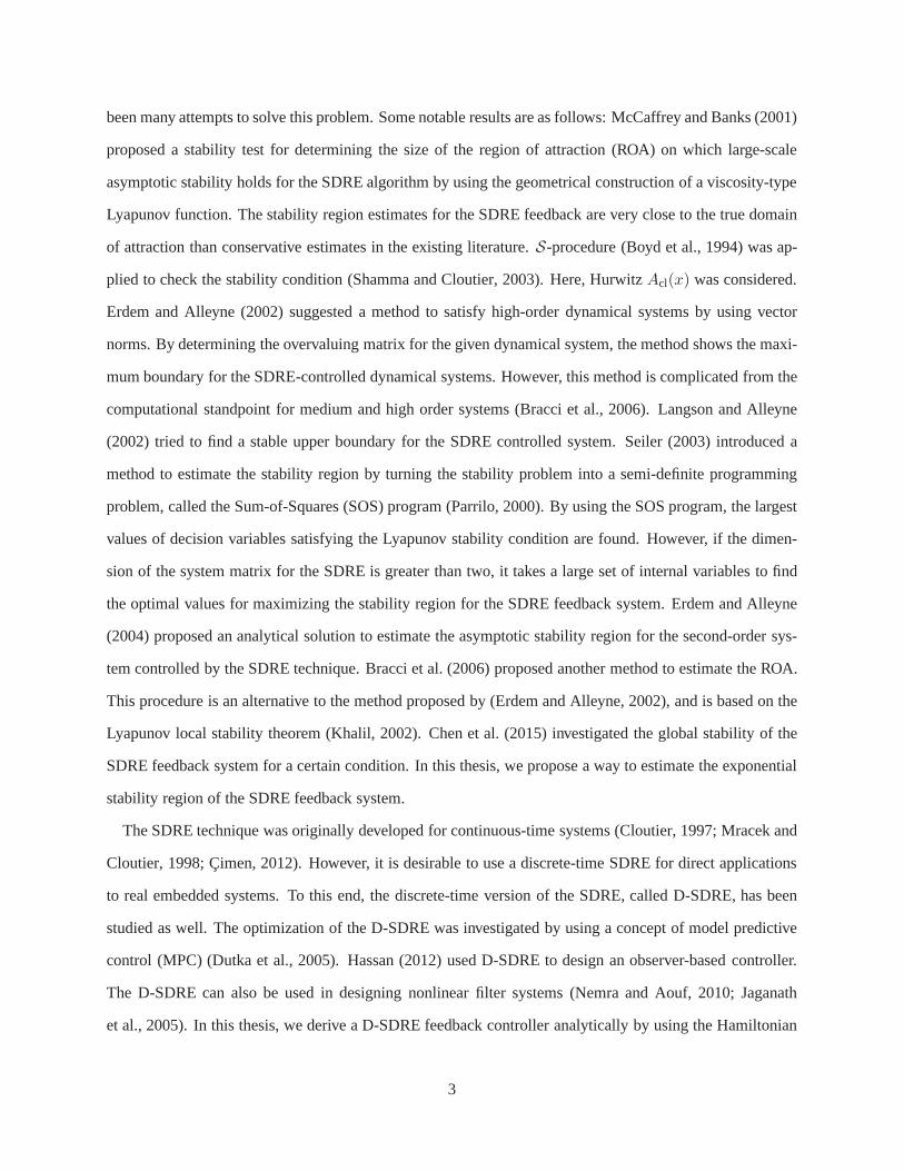
been many attempts to solve this problem. Some notable results are as follows: McCaffrey and Banks (2001)
proposed a stability test for determining the size of the region of attraction (ROA) on which large-scale
asymptotic stability holds for the SDRE algorithm by using the geometrical construction of a viscosity-type
Lyapunov function. The stability region estimates for the SDRE feedback are very close to the true domain
of attraction than conservative estimates in the existing literature.S-procedure (Boyd et al., 1994) was ap-
plied to check the stability condition (Shamma and Cloutier, 2003). Here, HurwitzAcl(x) was considered.
Erdem and Alleyne (2002) suggested a method to satisfy high-order dynamical systems by using vector
norms. By determining the overvaluing matrix for the given dynamical system, the method shows the maxi-
mum boundary for the SDRE-controlled dynamical systems. However, this method is complicated from the
computational standpoint for medium and high order systems(Bracci et al., 2006). Langson and Alleyne
(2002) tried to find a stable upper boundary for the SDRE controlled system. Seiler (2003) introduced a
method to estimate the stability region by turning the stability problem into a semi-definite programming
problem, called the Sum-of-Squares (SOS) program (Parrilo, 2000). By using the SOS program, the largest
values of decision variables satisfying the Lyapunov stability condition are found. However, if the dimen-
sion of the system matrix for the SDRE is greater than two, it takes a large set of internal variables to find
the optimal values for maximizing the stability region for the SDRE feedback system. Erdem and Alleyne
(2004) proposed an analytical solution to estimate the asymptotic stability region for the second-order sys-
tem controlled by the SDRE technique. Bracci et al. (2006) proposed another method to estimate the ROA.
This procedure is an alternative to the method proposed by (Erdem and Alleyne, 2002), and is based on the
Lyapunov local stability theorem (Khalil, 2002). Chen et al. (2015) investigated the global stability of the
SDRE feedback system for a certain condition. In this thesis, we propose a way to estimate the exponential
stability region of the SDRE feedback system.
The SDRE technique was originally developed for continuous-time systems (Cloutier, 1997; Mracek and
Cloutier, 1998; Çimen, 2012). However, it is desirable to use a discrete-time SDRE for direct applications
to real embedded systems. To this end, the discrete-time version of the SDRE, called D-SDRE, has been
studied as well. The optimization of the D-SDRE was investigated by using a concept of model predictive
control (MPC) (Dutka et al., 2005). Hassan (2012) used D-SDRE to design an observer-based controller.
The D-SDRE can also be used in designing nonlinear filter systems (Nemra and Aouf, 2010; Jaganath
et al., 2005). In this thesis, we derive a D-SDRE feedback controller analytically by using the Hamiltonian
3

(Bryson, Jr. and Ho, 1975) with state-dependent weighting matrices
The derivation and the analysis of the D-SDRE without and with constraints conditions, the latter named
constrained discrete-time state-dependent Riccati equation (CD-SDRE), are the main contributions of this
thesis. The constraint problem has been addressed through anti-windup (Kothare et al., 1994; Kothare
and Morari, 1999) and model predictive control (MPC) (Mayneet al., 2000; Rawlings and Mayne, 2009;
Grüne and Pannek, 2011). MPC has been applied to a linear quadratic regulation (LQR) under input/state
constraints (Scokaert and Rawlings, 1998; Bemporad et al.,2002; Johansen et al., 2002; Johansen, 2003;
Grieder et al., 2004; Ding et al., 2004; Lee and Khargonekar,2007; Zhao and Lin, 2008; Ferrante and
Ntogramatzidis, 2013). However, to the best of our knowledge, there are no specific results on SDRE (or
D-SDRE) with constraints on the inputs or states.
The CD-SDRE controller described above is for deterministic nonlinear systems. However, uncertainties
are ubiquitous in any systems. Therefore, the robustness ofthe CD-SDRE controller for such uncertain
nonlinear systems in the presence of constraints on the states/inputs should be investigated, which is another
main objective of the thesis. Based on the stability proof ofthe D-SDRE controller, we establish a robust
D-SDRE feedback controller, which is proven to be exponentially stable in its ROA. The linear matrix
inequalities (de Oliveira et al., 1999; Ramos and Peres, 2001) are used to prove the stability condition. The
stability analysis of the robust D-SDRE controller in the presence of constraints on the states/input, called a
robust CD-SDRE controller, is then investigated through the use of a concept of a switched system.
As a second part of the thesis, we investigate filtering techniques. The filtering techniques have been
one of the central topics in industry as well as academia for more than 50 years since online recursive
linear filters/observers were introduced in the 1960’s (Kalman, 1960; Kalman and Bucy, 1961; Luenberger,
1966). The filtering techniques have not only been a popular research topic but also been used as a crucial
application to control, estimation, optimization, and signal processing (Gelb, 1974; Bryson, Jr. and Ho,
1975; Anderson and Moore, 1979; Goodwin and Sin, 1984; Widrow and Stearns, 1985; Brown and Hwang,
1997; Doucet et al., 2000; Rawlings and Mayne, 2009; Lewis etal., 2012), just to name a few. Among
the various filtering techniques developed so far, the extended Kalman filter (EKF) has been one of the
main filtering techniques especially in industry since it issimple to design and easy to be implemented in a
system. However, stable operation has been a main problem inusing the EKF.
Other filtering techniques have emerged to overcome the weaknesses of the EKF. One of the notable
4
filtering techniques is the unscented Kalman filter (UKF) (Julier and Uhlmann, 1997, 2004). Unlike the
EKF, it does not use the lienarization such as Jacobian. Instead, it uses full nonlinear dynamical models
to propagate some meaningful samples called sigma points and estimates the states of the system from the
behaviors of the sigma points. Direct applicability of the nonlinear dynamical models gives high chances
to avoid the instability of the filtering systems. Unlike random particles in Monte Carlo method, the sigma
points are chosen deterministically so that they show certain mean and covariance (Julier and Uhlmann,
2004). Rao et al. (2003) investigated a filter design by meansof a concept of receding horizon in MPC
(Clarke et al., 1987a,b; Mayne et al., 2000), called the moving horizon estimator (MHE). Unlike EKF or
UKF which use only one step measurement to predict the statesfor the next step, MHE uses several prior
measurements and predicts the states for finite horizons by using a constrained optimization technique.
More accurate estimates of the states are expected than those by EKF or UKF (Rawlings and Mayne, 2009).
Sequential Monte Carlo (SMC) methods or particle filters (PF) were introduced to increase the accuracy of
the states especially in the presence of non-Gaussian noises in a system (Gordon et al., 1993). However, it
should be noted that UKF or PF use samples and MHE uses optimization technique. Moreover, the MHE
uses several measurement data and predicts states for finitehorizons while the Kalman filters predict only
one step ahead. These can cause significant computational burden in a system so that such a fact might limit
their applicability to various systems specifically in which fast sampling time or less computational power
are critical. Moreover, the performance of PF significantlydecreases as the dimension of the state increases.
It is also vulnerable to unmodeled disturbances (Rawlings and Mayne, 2009).
Another notable filtering technique is the state-dependentRiccati equation-based filter (SDREF), which
is based on the SDRE technique. Beside the SDRE technique specifically for the controller development,
the SDREF has also been investigated theoretically and applied to practical problems (Xin and Balakr-
ishnan, 2002; Jaganath et al., 2005; Çimen and Merttopçuoglu, 2008; Nemra and Aouf, 2010; Beikzadeh
and Taghirad, 2012b,a; Batmani and Khaloozadeh, 2012), to name a few. The SDREF can overcome the
linearization issue in EKF while it can also reduce the computational load which is a critical problem in
particle-based filters such as UKF or PF. However, more analytical analysis on the stability of the SDREF
should be studied. Moreover, most of the filtering techniques are designed under the assumption of Gaus-
sian noises. There might be many cases where noises in a system do not follow the normal distribution.
In these cases, PF is widely used. One of the strengths of the PF is the ability to estimate the state in the
5
presence of non-Gaussian noises while it has so called curseof dimensionality and is sensitive to ummod-
eled noises (Rawlings and Mayne, 2009). de Freitas et al. (2000) provided a filter by combining EKF and
PF to improve the performance of the PF. However, it still hasa linearization issue of the EKF part. van
der Merwe et al. (2000) tried to combine UKF and PF, called theunscented particle filter (UPF). Rawlings
and Mayne (2009) introduced a filter which contains MHE and PF. Although improved performance can be
expected from the filters, there is a trade-off: the computational burden will be increased due to the sigma
points in the UKF part and the longer horizons in the MHE part.In this thesis, we first start the discussion
with observer design through the use of the D-SDRE technique. Then, we propose a discrete-time version
of the SDREF, named D-SDREF. The proposed filter does not require the linearization like the EKF. It does
not need several samples as in UKF or PF. Thereby, it can reduce the computational burden while it can
estimate the real state values accurately. Then, a new filteris investigated by combining the D-SDREF and
PF so that the proposed filter can have the strengths of both filters.
1.2 Outline and Contributions
The main contributions of this thesis are:
In Part II, we discuss the CD-SDRE controllers for discrete-time nonlinear systems.
• In Chapter 5, we derive the D-SDRE feedback controller analytically by using the Hamiltonian
(Bryson, Jr. and Ho, 1975). To make the system more general, we allow weights on the perfor-
mance index to be minimized to be dependent on states while previous studies assumed that they are
constant or time-varying. Instead of using the discrete algebraic Riccati equation (DARE), a gener-
alized discrete-time Riccati equation is derived and used.By doing so, more accurate optimization
results can be expected since DARE’s assumption of steady-state conditions can lead to significant
errors in a controlled system. A condition for stability is proven by using the Lyapunov stability cri-
teria (Khalil, 2002). We suggest a way to find an ROA of the D-SDRE feedback system through the
use of linear matrix inequality (LMI) methods (Boyd et al., 1994; de Oliveira et al., 1999; Ramos and
Peres, 2001). We investigate the stability condition of theCD-SDRE feedback system as a switched
one due to the characteristics of the controller. We suggesttwo algorithms for CD-SDRE: a regulation
problem and a reference tracking problem. The analysis of the algorithms indicates that CD-SDRE
6

can perform in an optimal sense in the presence of the input/state constraints.
• In Chapter 6, the proposed CD-SDRE is evaluated by using challenging problems in spacecraft orbit
reconfiguration problems. We apply the proposed CD-SDRE controller to spacecraft orbit reconfig-
uration problems which have limited actuator performance.It is interesting to note that trajectory
optimization techniques have been widely used for the reconfiguration problems (Scharf et al., 2003,
2004). However, many of the previous studies show that the optimization techniques are based on
open-loop control methods which might be vulnerable to internal/external disturbances. Moreover,
most of them are not real-time trajectory optimizers. In order to overcome such problems, numerous
closed-loop tracking control methods have been suggested (Scharf et al., 2004). In this case, by using
a priori designed reference trajectories, the control methods calculate proper control signals to make
each spacecraft follows its reference. However, dependingon the size of orbits and initial conditions
(positions and velocities of spacecraft), excessively large initial control inputs might be inevitable in
the tracking control which are not desirable, since, in general, an actuator’s effort corresponding to
a large control signal cannot be generated by a real thrusterin a small spacecraft. Moreover, such
improper control signals can make the motions of the spacecraft unstable. Therefore, the actuator
saturation problem should be considered when designing a control system. Although the input sat-
uration problem is prevalent in real systems, many of the advanced control methods cannot take it
into account explicitly. For realistic results in this work, high-fidelity dynamical models of orbits
for the reference and deputy spacecraft are derived in the presence of the oblateness of the Earth (J2
perturbation) and atmospheric drag. The simulations show the reliable results by using the proposed
CD-SDRE technique.
• In Chapter 7, we extend our scope of the CD-SDRE technique to acase of controlling a class of uncer-
tain nonlinear system. A rigorous analysis of a robust state-feedback SDRE (or D-SDRE) controller
for uncertain nonlinear systems is investigated. The performance of the proposed robust CD-SDRE-
based feedback controller in the presence of uncertaintiesis evaluated through its application to the
attitude motion control of a spacecraft with a partially filled fuel tank. Unlike predictable disturbance
sources such as gravity-gradient/aerodynamic torques, magnetic fields, or solar radiation pressure,
the partially filled fuel tank can generate unwanted disturbances to the spacecraft: as the spacecraft
consumes fuel for orbit maintenance or momentum dumping, the volume of fuel in the tank shrinks.
7
Then, the rest of the fuel can generate a reaction force and excite spacecraft motion by using its
movement, called fuel slosh effect (Vreeburg, 2005; Bryson, Jr., 1994). It has been a challenging
problem for a long time and many researchers have tried to handle the disturbances (Peterson et al.,
1989; Agrawal, 1993; Vreeburg, 2005; Reyhanoglu and Hervas, 2011; Hervas et al., 2013). To bet-
ter address the fuel slosh effect, another objective of the thesis is to provide an accurate dynamical
model of a spacecraft attitude motion in 3-dimensional space in the presence of the effect. Most of
the previous studies listed above, especially for controlling the motion of the spacecraft, have focused
on a planar motion, i.e., 2-dimensional space, of a spacecraft, like a hovercraft, to investigate the fuel
slosh dynamics (Bryson, Jr., 1994; Reyhanoglu and Hervas, 2011; Hervas et al., 2013). The proposed
models might provide an insight of how to attenuate the disturbance. However, equations of motion
for this system have never been derived in 3-dimensional space, and simpler and less representative
2-dimensional models have been widely studied instead. Therefore, unlike the previous studies listed
above, we show the equations of motion in 3-dimensional space. Under the assumption of the first
fuel slosh mode (Bryson, Jr., 1994), the fuel can be considered as ice moving in the fuel tank. It is
interesting to note that it is analogous to motion of spacecraft which are connected by inelastic tethers
(Chang et al., 2010b).
In Part III, we investigate the design of the observer/filters based on the D-SDRE technique.
• In Chapter 8, we derive the D-SDRE-based observer for the deterministic nonlinear system. Detailed
procedure for deriving the D-SDRE Observer is provided by using a one-step process. The error
between the actual state and its corresponding estimated state via the D-SDRE Observer is studied
analytically to show its boundedness by using the input-to-state stability (ISS) analysis (Sontag, 1989;
Jiang and Wang, 2001). The D-SDRE Observer is evaluated by using the Lorenz attractor as an
example.
• In Chapter 9, one of the main contributions of the thesis in the filtering part, we investigate the
D-SDREF for stochastic nonlinear systems in the presence ofGaussian noises. First, we provide
detailed procedure for deriving the D-SDREF by using a two-step process with an assumption of
Gaussian noises. Theoretical proofs are provided to show that the state error between the measured
signal and the estimated one by the D-SDREF is ISS. The algorithm of the D-SDREF is provided.
8

The D-SDREF has several benefits compared to other filtering techniques. Unlike the EKF, the D-
SDREF does not need linearization of the stochastic system so that it can capture the nonlinearities
of the system. Moreover, it does not require demanding computational power since it does not use
many samples like UKF, MHE, or PF. or it only relies on the current states while the MHE uses longer
horizons (Rawlings and Mayne, 2009). In order to apply the D-SDREF to stochastic systems with
non-Gaussian distributed noises, we propose a new filter by combining the D-SDREF and PF, named
the combined D-SDRE/PF. The proposed filter has strengths and overcomes the weaknesses of both
filters. The proposed combined D-SDRE/PF can guarantee better performance than EKF/PF while
maintain lower computation cost than UPF or MHE/PF. We provide an algorithm of the combined
D-SDRE/PF. Finally, we evaluate the performance of the proposed D-SDREF and the combined D-
SDRE/PF by using challenging numerical examples: estimates of the states of the pendubot (Spong
and Block, 1995; Fantoni et al., 2000) and the Rössler attractor (Rössler, 1976; Pikovsky et al., 1996).
The proposed filtering techniques show outstanding performance to estimate accurate states while the
existing filtering techniques listed above have difficulty in estimating the states with high accuracy
compared to the proposed filters.
As independent studies which can provide good tools for the two parts listed above, a stability analysis of
the continuous-time SDRE feedback system is investigated.Moreover, we propose a gain-tuning algorithm
which can be widely applied to many practical problems as well as the CD-SDRE to estimate the parameters
in the MPC and D-SDRE.
• In Chapter 3, we discuss the exponential stability of the continuous-time SDRE feedback system and
how to estimate its ROA. The objective of the study is to estimate the exponential stability region for
the SDRE feedback systems by the motivation of contraction theory (Lohmiller and Slotine, 1998),
which is closely related to the incremental stability (Angeli, 2002) in the sense that both of them
consider the incremental dynamics for stability conditions. By applying the contraction analysis to
the SDRE controlled systems and interpreting it as polytopic linear differential inclusions (LDIs)
(Boyd et al., 1994), we can guarantee the exponential stability of the systems. Moreover, the stability
condition can be interpreted as an incremental exponentialstability, which has stronger characteristics
than exponential convergence (Pham et al., 2009). Furthermore, the ROA estimated by the proposed
method is an invariant set, which is essential because any trajectories starting from an invariant set
9

can be guaranteed to stay in it forever (Khalil, 2002).
• In Chapter 4, we investigate an automatic gain-tuning method, named the automatic-gain tuner via
the particle swarm optimization (AGT-PSO). The AGT-PSO calculates optimal values of user-defined
system parameters which is expected to be time/cost efficient and labor efficient in the sense that it
automatically tunes the system parameters with little background knowledge of the controller. More-
over, the performance of the system is shown to be significantly improved with the new parameters,
obtained by the AGT-PSO.
Chapter 2 provides some background material for this thesis.
10
Chapter 2
Preliminaries
THE basic schemes of the D-LQR, nonlinear MPC, and ISS are brieflyreviewed to help understand the
contents of the thesis. In this thesis, we use the following function classes. A functionγ : R≥0 → R≥0
is said to be of classK if it is continuous, strictly increasing, andγ(0) = 0. If γ is unbounded, it is
said to be of classK∞. A function β : R≥0 × R≥0 → R≥0 is said to be of classKL if β(·, k) is of
classK for each fixedk ≥ 0 andβ(ξ, k) is decreasing to zero ask → ∞ for each fixedξ ≥ 0. Some
notations are also defined which will be used throughout the thesis:N := 1, 2, 3, · · · ; Z≥0 := N ∪ 0;
Za:b := z ∈ N : z ≥ a, z ≤ b; a < b, a, b ∈ Z≥0; R := (−∞,+∞); R≥0 := r ∈ R : r ≥ 0.
2.1 Discrete-Time Linear Quadratic Regulator (D-LQR)
Suppose that there is a deterministic discrete-time lineartime-varying system described by the following
difference equation
xk+1 = Akxk +Bkuk, x(0) = x0 (2.1)
wherexk ∈ Rn anduk ∈ R
m are the state and the control input, respectively.
The objective of the D-LQR is to find the sequence of control inputsu0,u1, · · · ,uN−1 that minimizes the
performance index:
J0 =1
2
N−1∑
j=0
(
x⊤j Qjxj + u⊤
j Rjuj
)
(2.2)
whereQj andRj are assumed to be symmetric positive semi-definite and symmetric positive definite,
respectively.
To this end, we use the Hamiltonian as below (Lewis et al., 2012):
Hk =1
2
(
x⊤k Qkxk + u⊤
k Rkuk
)
+ λ⊤k+1
(
Akxk +Bkuk
)
(2.3)
11
whereλk ∈ Rn is the Lagrange multiplier.
Then, by using the optimality conditions (Bryson, Jr. and Ho, 1975), the controller can be designed as
uk = −R−1k B⊤
k λk+1 (2.4)
= −(B⊤
k P k+1Bk + P k
)−1B⊤
k P k+1Akxk, ∀k ∈ Z0:N−1
whereP k is the unique solution of the discrete-time Riccati equation at timek:
P k = Qk +A⊤k
(
P k+1 − P k+1Bk
(B⊤
k P k+1Bk +Rk
)−1B⊤
k P k+1
)
Ak. (2.5)
The detailed derivation of the D-LQR is omitted here since itis straightforward and can be found in (Lewis
et al., 2012; Kirk, 1970).
Remark 1 If the control horizon is consideredN → ∞, then (2.5) can be rewritten under the assumption
that the state of (2.1) has a steady-state value:
P = A⊤k
(
P − PBk
(B⊤
k PBk +Rk
)−1B⊤
k P)
Ak +Qk (2.6)
which is called the discrete-time algebraic Riccati equation (DARE). It is widely used in D-LQR problems.
2.2 Model Predictive Control
MPC is a main tool in the CD-SDRE technique to handle constraints on states and control inputs. We briefly
review the MPC in this section. More detailed information ofthe MPC can be found in (Mayne et al., 2000;
Rawlings and Mayne, 2009; Magni et al., 2009; Grüne and Pannek, 2011).
Consider a discrete-time nonlinear system described by thenonlinear difference equation:
xk+1 = f(xk,uk), x(0) = x0 ∀k ∈ Z≥0 (2.7)
wheref : X × U 7→ X maps the current statexk ∈ X ⊆ Rn and the current control inputuk ∈ U ⊆ R
m
into the successor statexk+1 ∈ X ⊆ Rn.
12
It is assumed that the system (2.7) is subject to hard constraints on the state and the control input:
uk ∈ U, xk ∈ X ∀k ∈ Z≥0 (2.8)
whereX ⊆ X, U ⊆ U , which are assumed to be closed and convex, are constraint sets of the state and the
control inputs, respectively.
Then, the purpose of MPC is to find a sequence of control inputsµ(·) ∈ U such that the following perfor-
mance index is minimized:
JN (x0,µ(·)) :=k+N−1∑
j=k
ℓ(xj ,uj) + Jf (xk+N ) (2.9)
s.t. xk ∈ X, uk ∈ U and (2.7) ∀k ∈ Z≥0
whereN is a finite horizon andℓ(·) is assumed to be continuous withℓ(0,0) = 0.
Therefore, by solving the optimal control problem, the optimal state and control sequence as functions of
the initial statex0 and timek can be obtained;µ = [u⊤(0) u⊤(1) · · · u⊤(N − 1)]⊤ ∈ RNm is the
optimization vector. In MPC, the first element in the optimalcontrol actionµ(·) is chosen for the control
input at timek, i.e.,uk = µ(0) becomes the control input signal at timek, and the sequence is repeated for
the next time step.
Remark 2 The constraints in (2.8) at timek can be expressed in the following matrix form
Mµ ≤W + Sxk. (2.10)
Then, the minimization of (2.9) becomes the convex quadratic programming (QP). The QP is widely used
in MPC.
2.3 Input-to-State Stability
We introduce the concept of input-to-state stability (ISS)(Sontag, 1989; Jiang and Wang, 2001) which is
used throughout the thesis.
13
Definition 1 (Jiang and Wang, 2001) The discrete-time nonlinear system
xk+1 = f(xk,uk) (2.11)
is said to be input-to-state stable (ISS) if there existβ ∈ KL, γ ∈ K, and constantη1, η2 ∈ R≥0 such that
|xk| ≤ β(|x0|, k) + γ(|u|L∞) ∀k ∈ Z≥0 (2.12)
for all x0 ∈ X anduk ∈ U satisfying that|x0| < η1 and |u|L∞< η2.
Definition 2 (Jiang and Wang, 2001) A continuous functionV : Rn → R≥0 is said to be an ISS-Lyapunov
function for (2.11) if the following hold:
1. There existα1, α2 ∈ K∞ such that
α1(|ξ|) ≤ V (ξ) ≤ α2(|ξ|) ∀ξ ∈ Rn. (2.13)
2. There existα3 ∈ K∞ andσ ∈ K such that
V (f(ξ,µ))− V (ξ) ≤ −α3(|ξ|) + σ(|µ|) (2.14)
for all ξ ∈ Rn andµ ∈ R
m.
14
Chapter 3
Exponential Stability Region Estimates forthe Continuous-Time SDRE
A S a preliminary of the thesis, we investigate the exponentialstability of the continuous-time state-
dependent Riccati equation-based control. Some notable prior work has shown local asymptotic
stability of SDRE by using numerical and analytical methods. In this chapter, we introduce a new strategy,
based on contraction analysis and incremental stability analysis, to estimate the exponential stability region
for the SDRE controlled system. Examples demonstrate the superiority of the proposed method.
The organization of this chapter is as follows: preliminaries of the continuous-time SDRE control, a brief
introduction to contraction analysis are presented in Section 3.1. The stability proof of the SDRE controlled
systems is described in Section 3.2. In Section 3.3, two numerical examples are presented to compare the
results with other numerical methods. Finally, concludingremarks are stated in Section 3.4.
3.1 Preliminaries
3.1.1 State-Dependent Riccati Equation Technique
Consider a deterministic, infinite-horizon nonlinear optimal regulation problem, where the system is full-
state observable, autonomous, nonlinear in the state, and affine in the input, represented in the form (Çimen,
2008)
x(t) = f(x) +B(x)u(t), x(0) = x0 (3.1)
wherex ∈ Rn is the state vector andu ∈ R
m is the input vector.
The SDRE technique is a nonlinear control design method for the direct construction of nonlinear feed-
back controllers. Through the state-dependent coefficient(SDC) factorization, system designers can rep-
resent the nonlinear equations of motion as linear structures with state-dependent coefficients. Then, the
LQR technique can be applied to this state-dependent state-space equation. Thus, the following procedure
15
is similar to the LQR method, except that all matrices may depend on the states. Based on this concept, the
state-space equation for the nonlinear system described in(3.1) can be expressed as a linear-like state-space
equation using the direct SDC factorization as:
x = A(x)x+B(x)u (3.2)
where the factorization forf(x) = A(x)x is possible if and only iff(0) = 0 andf(x) is continuously
differentiable. Note thatA(x) is not a unique matrix because there could be many possible choices in the
direct SDC factorization (Cloutier, 1997). For this system, the SDRE technique finds an inputu(t) that
approximatelyminimizes the following performance index:
J =1
2
∫ ∞
0
(
x⊤Q(x)x+ u⊤R(x)u)
dt (3.3)
whereQ(x) is a symmetric positive semi-definite matrix with quadraticform andR(x) is a symmetric
positive definite matrix with quadratic form for allx ∈ Rn. Also, it is assumed thatf(0) = 0 and
B(x) 6= 0. It should be noted thatQ(x) andR(x) are not only allowed to be constant, but can also be
varied as functions of states. As these state-dependent matrices are applied to the algebraic Riccati equation
(ARE), the following state-dependent Riccati equation is obtained (Cloutier, 1997):
P (x)A(x) +A⊤(x)P (x) +Q(x)
−P (x)B(x)R−1(x)B⊤(x)P (x) = 0 (3.4)
The optimal feedback control gain matrix, which is a state-dependentm×n variable gain matrix, and the
m×1 input control can be calculated in the same way as the LQR technique except for the state dependence:
K(x) = R−1(x)B⊤(x)P (x) (3.5)
u = −K(x)x
whereP (x) ∈ Rn×n is the unique positive-definite solution of the SDRE (3.4).
As with the LQR technique, the SDRE technique also constructs a closed-loop system with direct state
16

feedback controlleru(t) as a regulator. However, the feedback gain,K(x), of the SDRE technique de-
pends on the states. Hence, state-dependent control inputsare applied to the plant. Because the state-space
equation (3.2) should be computed for every state and control input, (3.4) and (3.5) should be calculated
at each time step. Because the SDRE technique can be considered as the LQR method for each time step,
the matrixP (x) in (3.4) becomes a unique solution of the algebraic Riccati equation at the particular state,
x(t), which means it has constant values at each given state. Therefore, solving the ARE in (3.4) for each
x is feasible and can be done either on-line or off-line (Erdem, 2001).
Controllability is critical because it is a sufficient condition for the existence of a solution to the SDRE. In
general, a linear time-invariant system is controllable ifand only if then× nm controllability matrixW ctrl
has full rank (i.e.,rank(W ctrl) = n). The controllability of the SDRE can be determined by pointwise
controllability (W ctrl(x)) of the SDC factorization
W ctrl(x) =[B(x) A(x)B(x) A2(x)B(x) · · · An−1(x)B(x)
]. (3.6)
Thus, the selection of (A(x) andB(x)) can affect the controllability of the system.
3.1.2 Contraction Theory
The new method proposed in this chapter is motivated by contraction analysis, a relatively new nonlinear
stability tool for exponential stability for the nonlinearsystems. It is a generalized version of Krasovskii’s
theorem (Khalil, 2002), which provides a sufficient, asymptotic convergence result. Readers are referred to
(Lohmiller and Slotine, 1998) for more detailed information about contraction analysis.
Consider a general deterministic system of the form
x(t) = f(x,u(x, t), t) (3.7)
wheref : Rn×Rm×R 7−→ Rn is a nonlinear vector function andx ∈ R
n is the state vector. This nonlinear
system can be thought of as ann-dimensional fluid flow, wherex is then-dimensional “velocity” vector at
then-dimensional positionx and timet. Assuming thatf(x,u(x, t), t) is continuously differentiable, the
17
exact differential relation can be obtained by (3.7):
δx(t) =∂f
∂x(x,u(x, t), t)δx (3.8)
whereδx is a virtual displacement of the systems. Note thatδx defines a linear tangent differential form,
andδx⊤δx the associated quadratic tangent form, both of which are differentiable with respect to timet.
Consider two neighboring trajectories in the flow field (3.7), and the virtual displacementδx between
them. The squared distance (quadratic virtual length) between these two trajectories can be defined as
δx⊤δx, leading from (3.8) to the rate of change
ddt(δx⊤δx) = 2δx⊤δx = 2δx⊤∂f
∂xδx. (3.9)
Denoting byλmax(x, t) the largest eigenvalue of the symmetric part of the Jacobian∂f∂x , we have
ddt(δx⊤δx) ≤ 2λmaxδx
⊤δx (3.10)
and hence,
‖δx‖ ≤ ‖δx0‖e∫ t0 λmax(x,t)dt (3.11)
Assuming thatλmax is uniformly strictly negative, then from (3.11) any infinitesimal length‖δx‖ con-
verges exponentially to zero.
3.1.3 Generalized Contraction Analysis
The line vectorδx defined in (3.8) can also be expressed using the differentialcoordinate transformation
(Lohmiller and Slotine, 1998), and leads to a generalization of the previous definition of squared length as
δz = Θ(x, t)δx,
δz⊤δz = δx⊤Mδx(3.12)
whereΘ(x, t) andM = Θ⊤Θ denote a square matrix and a symmetric and continuously differentiable
metric, respectively. Therefore, exponential convergence of δz to 0 implies exponential convergence ofδx
to 0.
18

The time derivative ofδz = Θδx can be computed as
ddtδz = Θδx+Θδx (3.13)
=
(
Θ+Θ∂f
∂x
)
Θ−1δz , Hδz.
The rate of change of squared length can be written
ddt(δz⊤δz) = 2δz⊤Hδz. (3.14)
Therefore, if there exists aγ > 0, such that the symmetric part ofH is negative definite, that is,
H +H⊤
2< −γI, (3.15)
then the system is exponentially stable. It is helpful to recall thatH = H(x, t).
By using the characteristics of contraction analysis, we will estimate the exponential stability region for
the SDRE controlled systems in the next section.
3.2 Exponential Stability Analysis of the SDRE Feedback Systems
Given the nonlinear equation (3.1) under the assumption of an autonomous nonlinear equation, the equation
can be rewritten in the form (3.2) by applying the SDC factorization. Moreover, by applying the control law
(3.5) to the SDC factorization, the closed-loop form can be obtained as
x =(A(x)−B(x)K(x)
)x
=(A(x)−B(x)R−1(x)B⊤(x)P (x)
)x
=: Acl(x)x. (3.16)
Furthermore, for simplicity, (3.16) can be written asx = φ(x). Note thatφ(x) ∈ G whereG =
Coφ1, φ2, · · · , φk is polytopic LDIs (Boyd et al., 1994). Here,φi is obtained by an associatedxi.
Then for anyx in its ROAX , the following system describes the dynamics of the virtualdisplacementδx
19
of the system (3.16),ddt(δx⊤δx) = 2δx⊤δx = 2δx⊤F δx (3.17)
whereF := ∂φ∂x = Acl(x) +
∂∂xAcl(x)x denotes a Jacobian of the system (3.16).
Now we define a new term below:
Definition 3 The system (3.16) is said to be locally incrementally exponentially stable (IES) with an ROA
X ⊂ Rn if the system (3.17) is locally exponentially stable when initial condition of any two neighboring
trajectories, sayxl(t0) andxm(t0), are inX such thatδx(t0) = xl(t0)− xm(t0).
By the definition, if the system (3.16) is locally IES withX , then
ddt(δx⊤δx) ≤ −2λδx⊤δx and ‖δx‖ ≤ ‖δx0‖e−
∫ t0 λ(x,t)dt (3.18)
hold for any two neighboring trajectoriesxl(·) andxm(·) withxl(t0) andxm(t0) both inX . Here,λ(x, t) >
0 is the smallest eigenvalue of the symmetric part of the Jacobian F in (3.17). Note that (3.18) clearly
indicates thatδx will converge to zero exponentially with the convergence rateλ.
The below theorem shows a condition of the locally IES ROA of nonlinear systems controlled by the
SDRE technique.
Theorem 4 For the system (3.16), suppose that there existM = M⊤ > 0 and α > 0, such that the
following matrix inequality holds
MF i + F⊤i M + 2αM ≤ 0. ∀i = 1, 2, · · · , k (3.19)
whereF i :=∂φi
∂x andF i ∈ F := CoF 1, F 2, · · · , F k, whereF is a polytope. Note thatF ∈ F . Then
the system (3.16) is locally IES with an ROAX if X = E(M ,ρ, r) is an invariant set for the system (3.16),
whereE(M ,ρ, r) := x : (x− ρ)⊤M(x− ρ) ≤ r2.
Proof SinceX is an invariant set for the system (3.16), any trajectories of this system with its initial state
in X stays inX for all times. Consider the system described by (3.16) withxl(t0) andxm(t0) both inX ,
which implies that bothxl(t) andxm(t) are inX for all t ≥ t0. Then by pre and post-multiplying (3.19)
20
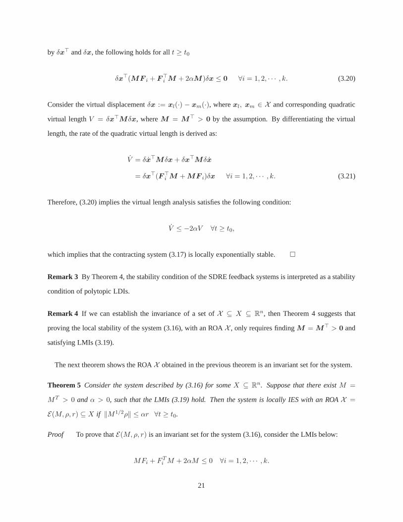
by δx⊤ andδx, the following holds for allt ≥ t0
δx⊤(MF i + F⊤i M + 2αM )δx ≤ 0 ∀i = 1, 2, · · · , k. (3.20)
Consider the virtual displacementδx := xl(·) − xm(·), wherexl, xm ∈ X and corresponding quadratic
virtual lengthV = δx⊤Mδx, whereM = M⊤ > 0 by the assumption. By differentiating the virtual
length, the rate of the quadratic virtual length is derived as:
V = δx⊤Mδx+ δx⊤Mδx
= δx⊤(F⊤i M +MF i)δx ∀i = 1, 2, · · · , k. (3.21)
Therefore, (3.20) implies the virtual length analysis satisfies the following condition:
V ≤ −2αV ∀t ≥ t0,
which implies that the contracting system (3.17) is locallyexponentially stable.
Remark 3 By Theorem 4, the stability condition of the SDRE feedback systems is interpreted as a stability
condition of polytopic LDIs.
Remark 4 If we can establish the invariance of a set ofX ⊆ X ⊆ Rn, then Theorem 4 suggests that
proving the local stability of the system (3.16), with an ROAX , only requires findingM = M⊤ > 0 and
satisfying LMIs (3.19).
The next theorem shows the ROAX obtained in the previous theorem is an invariant set for the system.
Theorem 5 Consider the system described by (3.16) for someX ⊆ Rn. Suppose that there existM =
MT > 0 andα > 0, such that the LMIs (3.19) hold. Then the system is locally IES with an ROAX =
E(M,ρ, r) ⊆ X if ‖M1/2ρ‖ ≤ αr ∀t ≥ t0.
Proof To prove thatE(M,ρ, r) is an invariant set for the system (3.16), consider the LMIs below:
MFi + F Ti M + 2αM ≤ 0 ∀i = 1, 2, · · · , k.
21
Post and pre-multiplying the above LMI byδx and its transpose, the inequality can be obtained
δxT (MFi + F Ti M + 2αM)δx ≤ 0 ∀i = 1, 2, · · · , k. (3.22)
If there existsρ ∈ Rn such thatδxTMρ ≥ 0, then (3.22) can be rewritten with the definition ofV :=
δxTMδx as
V ≤ −2αV + 2δxTMρ. (3.23)
Now, lets := ‖M1/2δx‖ andσ := ‖M1/2ρ‖. Note thatV = s2 andσ ≤ αr. By substitutings andσ into
(3.23), then
V ≤ −2αs2 + 2sσ ≤ −2αs (s− r) . (3.24)
Sinceα > 0, the above inequality implies thatV < 0 ∀s > r. This implies thatV ≤ r2 is an invariant
ellipsoid for the system ofδx. This indicates thatE(M,ρ, r) is an invariant set for the system (3.16).
Remark 5 If an ROA X ∈ X for a certain system is satisfied with Theorems 4 and 5, the ROAis an
invariant set.
We proved the exponential stability condition of SDRE feedback systems and shows how to estimate the
ROA. In the next section, the stability analysis will be evaluated with some numerical examples.
3.3 Numerical Validation
In this section, the exponentially stability analyses of two nonlinear systems controlled by the SDRE are
examined. The first example is a simple second order nonlinear system (Shamma and Cloutier, 2003) and
the other is attitude control of the aircraft (Etkin, 1972).Please note that an estimation method in (Bracci
et al., 2006) is shown to be more accurate than prior studies.Hence, the simulation results of the proposed
method in this chapter are compared with those by Bracci et al. (2006).
22
3.3.1 Case Study I: Second Order Nonlinear System
The first example is for a simple second order nonlinear feedback control system (Shamma and Cloutier,
2003). Consider the second-order nonlinear system:
x = A(x)x+Bu =
x1 1
0 0
x+
0
1
u. (3.25)
For simplicity, let us assume that the weighting matricesQ(x) andR(x), which are used in the algebraic
Riccati equation as well as in the Lypunov equation for the method by Bracci et al. (2006), are constant such
thatQ = diag(100, 100) andR = 1, respectively.
For estimation of the exponentially stable ROAX ⊂ R2, the Jacobian of the nonlinear system (3.25),
used in the virtual length analysis, can be obtained by (3.17). Now, let us define a convex setX ∈ R2. Then
the exponentially stable region can be estimated. That is, if there existM = M⊤ > 0, α > 0, such that
(3.19) holds, then (3.25) is exponentially stable with an ROA X ⊆ X ⊂ R2.
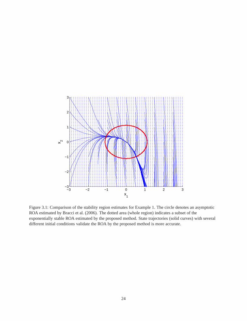
Figure 3.1 shows simulation results of the ROAs by the methodby Bracci et al. (2006) and the proposed
method. The circle in Figure 3.1 denotes the ROA estimated byBracci et al. (2006). The dotted area shows
the subset of the exponentially stable ROA for the system, obtained by the proposed method. Apparently,
the exponentially stable region is global inxi ∈ [−3, 3], i = 1, 2. Several state trajectories with different
initial conditions are shown in Figure 3.1 (solid curves). Here, one can easily notice that even some state
trajectories, which start from unstable region by the method by Bracci et al. (2006), still converge to the
equilibrium pointxe = 0. By the state trajectories, we can see the ROA estimated by the proposed method
is more accurate.
The next simulation shows a more complicated example: an attitude control system of an aircraft.
23
−3 −2 −1 0 1 2 3−3
−2
−1
0
1
2
3
x1
x 2
Figure 3.1: Comparison of the stability region estimates for Example 1. The circle denotes an asymptoticROA estimated by Bracci et al. (2006). The dotted area (wholeregion) indicates a subset of theexponentially stable ROA estimated by the proposed method.State trajectories (solid curves) with severaldifferent initial conditions validate the ROA by the proposed method is more accurate.
24
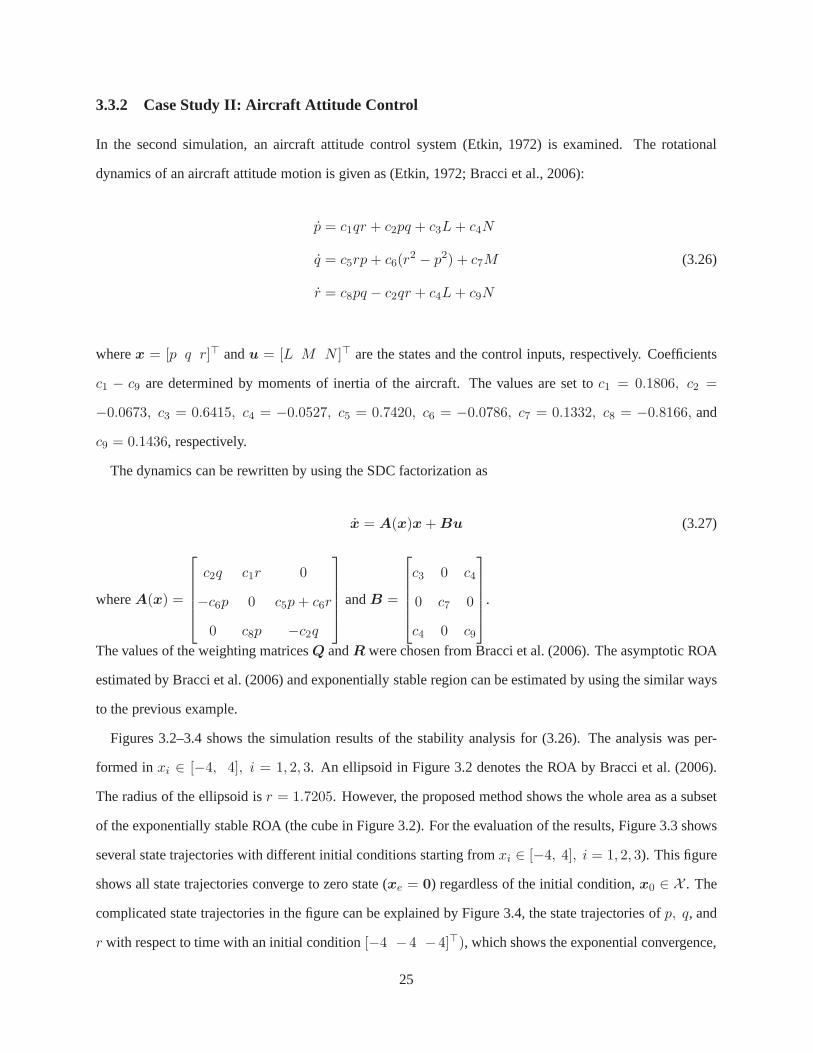
3.3.2 Case Study II: Aircraft Attitude Control
In the second simulation, an aircraft attitude control system (Etkin, 1972) is examined. The rotational
dynamics of an aircraft attitude motion is given as (Etkin, 1972; Bracci et al., 2006):
p = c1qr + c2pq + c3L+ c4N
q = c5rp+ c6(r2 − p2) + c7M (3.26)
r = c8pq − c2qr + c4L+ c9N
wherex = [p q r]⊤ andu = [L M N ]⊤ are the states and the control inputs, respectively. Coefficients
c1 − c9 are determined by moments of inertia of the aircraft. The values are set toc1 = 0.1806, c2 =
−0.0673, c3 = 0.6415, c4 = −0.0527, c5 = 0.7420, c6 = −0.0786, c7 = 0.1332, c8 = −0.8166, and
c9 = 0.1436, respectively.
The dynamics can be rewritten by using the SDC factorizationas
x = A(x)x+Bu (3.27)
whereA(x) =
c2q c1r 0
−c6p 0 c5p+ c6r
0 c8p −c2q
andB =
c3 0 c4
0 c7 0
c4 0 c9
.
The values of the weighting matricesQ andR were chosen from Bracci et al. (2006). The asymptotic ROA
estimated by Bracci et al. (2006) and exponentially stable region can be estimated by using the similar ways
to the previous example.
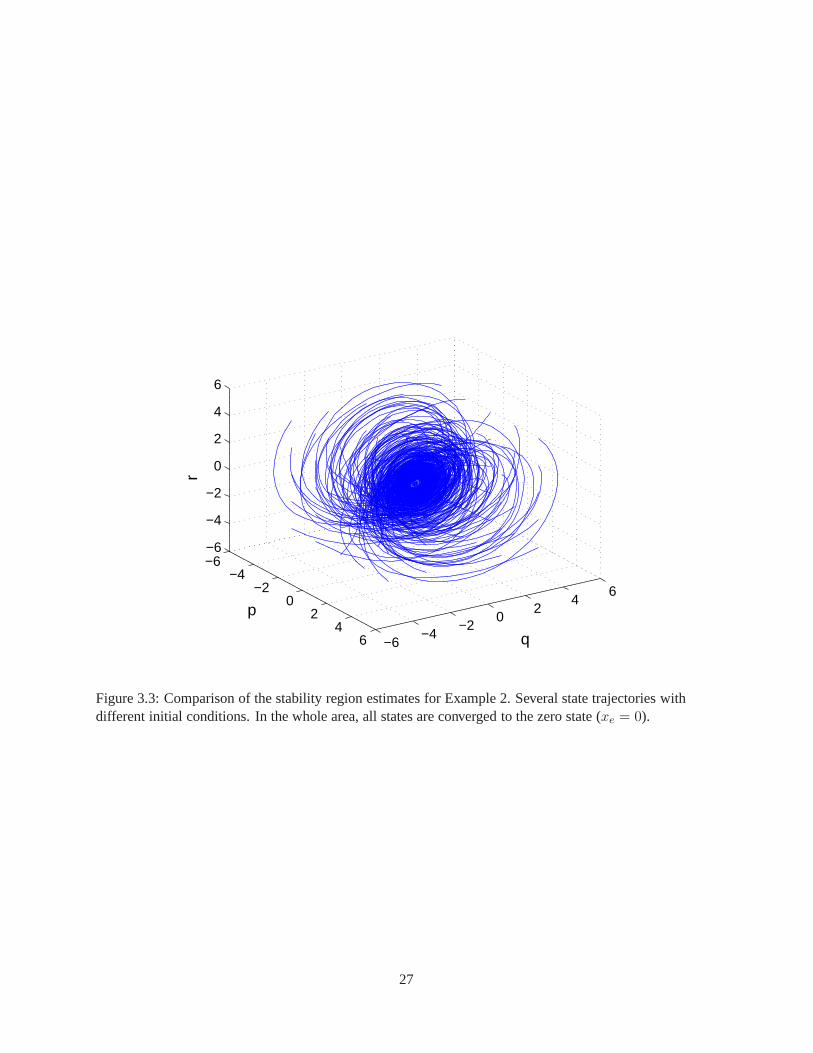
Figures 3.2–3.4 shows the simulation results of the stability analysis for (3.26). The analysis was per-
formed inxi ∈ [−4, 4], i = 1, 2, 3. An ellipsoid in Figure 3.2 denotes the ROA by Bracci et al. (2006).
The radius of the ellipsoid isr = 1.7205. However, the proposed method shows the whole area as a subset
of the exponentially stable ROA (the cube in Figure 3.2). Forthe evaluation of the results, Figure 3.3 shows
several state trajectories with different initial conditions starting fromxi ∈ [−4, 4], i = 1, 2, 3). This figure
shows all state trajectories converge to zero state (xe = 0) regardless of the initial condition,x0 ∈ X . The
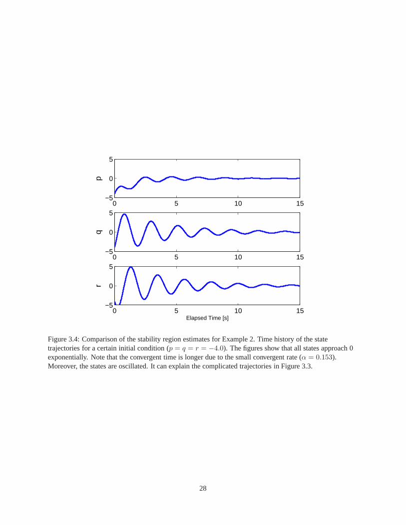
complicated state trajectories in the figure can be explained by Figure 3.4, the state trajectories ofp, q, and
r with respect to time with an initial condition[−4 −4 −4]⊤), which shows the exponential convergence,
25

−4−2
02
4 −4−2
02
4
−4
−2
0
2
4
qp
r
Figure 3.2: Comparison of the stability region estimates for Example 2. ROA by Bracci et al. (2006)(ellipsoid,r = 1.7205) and ROA by the proposed method (cube, whole area(subset))
26
−6−4
−20
24
6 −6−4
−20
24
6
−6
−4
−2
0
2
4
6
q
p
r
Figure 3.3: Comparison of the stability region estimates for Example 2. Several state trajectories withdifferent initial conditions. In the whole area, all statesare converged to the zero state (xe = 0).
27
0 5 10 15−5
0
5
p
0 5 10 15−5
0
5
q
0 5 10 15−5
0
5
Elapsed Time [s]
r
Figure 3.4: Comparison of the stability region estimates for Example 2. Time history of the statetrajectories for a certain initial condition (p = q = r = −4.0). The figures show that all states approach 0exponentially. Note that the convergent time is longer due to the small convergent rate (α = 0.153).Moreover, the states are oscillated. It can explain the complicated trajectories in Figure 3.3.
28
although it shows the oscillatory motions of the states.
From the two examples, the superiority of the proposed method for estimating the exponentially stable
ROA for the SDRE feedback systems is apparent. Note that the proposed method provides more accurate
information than the prior work, so that the results could bemore reliable.
3.4 Conclusions
We proposed a new method to estimate an ROA for the nonlinear system controlled by the SDRE controllers.
The proposed method estimates the exponentially stable ROAfor the SDRE feedback systems, while pre-
vious relevant work estimated the asymptotically stable ROAs in a conservative manner. The proposed
method considers the contraction analysis, the incremental stability analysis, and the LMIs, specifically
polytopic LDIs for the stability condition. Estimated ROAsby the method can be expected more accurate
than those by prior studies. Through two examples, we demonstrated the reliability of the proposed method
for estimating the ROA for nonlinear SDRE feedback systems.
29
Chapter 4
Automatic Gain-Tuner via Particle SwarmOptimization
I N this chapter, we discuss an automatic gain tuning system, named the automatic gain-tuner via parti-
cle swarm optimization technique (AGT-PSO). The AGT-PSO calculates optimal values of user-defined
system parameters which is expected to be time/cost efficient and labor efficient in the sense that it auto-
matically tunes the system parameters with little background knowledge of the controller. Moreover, the
performance of the system is shown to be significantly improved with the new parameters, obtained by the
AGT-PSO. Even without any prior knowledge about control systems to be designed, system designers can
tune the parameters of the controllers, which could have various forms, through the use of the AGT-PSO. It
can be used to evaluate the existing control setups and will show suboptimal values of the parameters de-
pending on the current setups. Examples with heavy industrymachine tuning tools show the effectiveness
and the reliability of the AGT-PSO.
4.1 Introduction
In modern society, structures of machines are becoming moresophisticated due to high demands such as
fast response, fine accuracy, improved robustness, etc. Forthese systems to be feasible, several types of
techniques of control and estimation should be used. Therefore, the overall structure of the control system
may have a complex multi-loop. As the control system gets more complicated, the more gains or gains
with more constraints may be used. In this case, tuning the gains might be a challenging problem since tun-
ing a complex multi-loop control system or hierarchical structure requires considerable experience (Zhang
et al., 2012). Unfortunately, however, the number of available qualified control engineers has decreased in
today’s industry although well trained engineers’ skills become more important and there is a great need for
high-fidelity tuning tools to maintain and improve the performance of complex control systems. Moreover,
30
although proportional-integral-derivative (PID) controllers are widely used in industry due to their sim-
plicity and robustness in some sense, it is essential to consider new controllers for improved performance.
Therefore, it is essential to develop automatic gain tuningmethods so that they can replace experienced
engineers and reduce time-cost to find “good” gains for the complex control systems.
The purpose of the current chapter is to investigate an automatic and simultaneous gain tuning algorithm
for complex systems, especially for industrial machines. There is large volume of research on the automated
tuning algorithms. First of all, several automatic tuning methods for PID-based controllers have been widely
discussed in (Åström et al., 1993; Johnson and Moradi, 2005), and references therein. Crowe et al. (2003)
studied the possibility of tuning PID controllers by using anew model-free gain tuning method, called the
controller parameter cycling method. Kim et al. (2010) proposed a tuning method for a PID controller by
using recursive least-square with linearization, which isexpected to show fast response and good overall
performance. Scaling and bandwidth-parameterization were also used to tune gains of a PID controller
(Gao, 2003). A relay feedback technique was used in designing a PID controller for DC–DC converters
(Stefanutti et al., 2007). A model-free gradient based tuning algorithm, called iterative feedback tuning
(IFT), was extensively studied by (Hjalmarsson et al., 1998; Hjalmarsson, 2002) and references therein.
Lequin et al. (2003) compared IFT with a conventional methodfor tuning PID controllers. Zhang et al.
(2012) tuned a PID cluster controller for a boiler/turbine system through the use of IFT.
One might notice that the major target of the automatic gain tuning systems listed above is a PID-based
controller. A reason of using such fixed gain controllers in industry is to avoid the possible abuse of adaptive
schemes, which is more complicated than a fixed gain controller (Tan et al., 2002). However, there have been
many attempts to apply different types of controllers to theexisting systems such as linear quadratic regu-
lator (LQR), linear quadratic Gaussian (LQG) control, gainscheduling, adaptive control, model predictive
control, etc. Even in this case, there are gains and system parameters to be tuned. Therefore, it is essential
to find “good” values of the parameters for reasonable performance of the system. For this, Sánchez et al.
(2004) used a subspace identification method for a tuning algorithm which is for multivariable restricted
structure control systems. A simultaneous perturbation stochastic approximation (SPSA) was used in multi-
variate stochastic approximation (Spall, 1992) and it was implemented in (Spall, 1998). As a direct method
for constructing feedback controller, virtual reference feedback tuning (VRFT) for a linear system (Campi
et al., 2002) and a nonlinear system (Campi and Savaresi, 2006) were investigated, respectively. As an
31
application, Radac et al. (2011) applied IFT and SPSA to servo system control. By using the correlation
method, iterative schemes (Karimi et al., 2004) and non-iterative schemes (Karimi et al., 2007) were studied
for tuning controllers. However, most of the approaches listed above are related to gradient-based methods.
Therefore, it might not be able to show optimized parameter values if a cost function to be minimized is
neither convex nor smooth or the system has constraints on inputs or outputs. Therefore, these issues should
be taken into account in the new gain tuning algorithms.
The main objective of the chapter is to show an automatic tuning algorithm of a controller of a complex
system by using a global optimizer, particle swarm optimization (PSO), named as the automatic gain-tuner
via PSO (AGT-PSO). The PSO, first introduced by Kennedy and Eberhart (1995), is a heuristic optimization
algorithm, based on a swarm intelligence. It was developed through a simulation of a simplified social
behavior, and was found to be robust in solving nonlinear optimization problems (Shi and Eberhart, 1998).
Constraints can be included in finding optimal solutions in PSO (Parsopoulos and Vrahatis, 2002). The PSO
technique can generate high-fidelity results with less calculation time and stable convergence characteristic
than other stochastic methods such as genetic algorithms (GA) and simulated annealing (SA) (Eberhart
and Shi, 1998; Gaing, 2004; Hassan et al., 2005). PSO also guarantees its reliability in non-smooth cost
functions (Park et al., 2005). Due to the superiority of PSO,it has been widely applied to industrial as well
as academic problems. For applications of a PID controller,Zhang et al. (2010) compared PSO, GA, and
SA to tuning PID clusters for a boiler/turbine system. Convergence analysis and parameter selection of PSO
were studied in (Trelea, 2003). Gaing (2004) applied PSO to find an optimal PID controller in an automatic
voltage regulator system. Constrained PSO was investigated to design a PID controller (Kim et al., 2008).
The performance of feedback linearization control for an industrial heavy machine was compared by using
IFT and PSO (Bentsman et al., 2012). Applicability of PSO to tuning parameters of more sophisticated
controllers such as gain scheduling,L1 adaptive control, limiting control, etc. was investigated(Chang
et al., 2013), which showed overall significant improvementof the performance when using PSO.
We can summarize the contributions as follows:
• Unlike the existing tuning methods listed above, AGT-PSO can be applied to designing not only
PID controllers but it can also be used to find optimal setups for various types of linear/nonlinear
controllers. Moreover, AGT-PSO can be a useful tool for identification of open-loop and closed-loop
systems.
32
• Unlike gradient-based tuning algorithms such as IFT and SPSA, AGT-PSO can obtain optimized so-
lutions of the controlled systems even with non-smooth or non-convex cost functions due to the char-
acteristics of PSO (Parsopoulos and Vrahatis, 2002; Park etal., 2005; Selvakumar and Thanushkodi,
2007; Niknam, 2010). It is of significant importance in industry due to the fact that such cost func-
tions are common in industrial machines because of the complexity of the systems and constraints on
inputs/outputs.
• AGT-PSO can obtain optimal values of a complex control system with shorter calculation time than
those by heuristic methods, i.e., trial-and-error methods, which is the most common method of tuning
system parameters in industry (Zhang et al., 2012). Moreover, the performance of the system can be
improved significantly with AGT-PSO.
• Any prior knowledge of a control system is not needed to applyAGT-PSO to tuning parameters of the
system. Moreover, control designers can use AGT-PSO not only to find optimal values of the gains
without any prior knowledge (i.e., a wild initial guess is acceptable.) but also to verify optimality of
the given initial setup of the gains.
• The existing optimizer, PSO, can be replaced with other optimization tools such as GA and SA de-
pending on system designer’s preference.
The organization of this chapter is as follows: The algorithm of AGT-PSO is introduced together with
a brief introduction of PSO in Section 4.2. Subsequently, the performance of AGT-PSO is evaluated by
applying it to two industrial examples in Section 4.3. Finally, conclusions are presented at the end of the
chapter.
4.2 Automatic Gain-Tuner via Particle Swarm Optimization (AGT-PSO)
In AGT-PSO, an optimization technique plays a crucial role and PSO is used as the optimization tech-
nique. In this section, AGT is introduced together with a brief introduction of PSO. Readers are referred to
(Kennedy and Eberhart, 1995; Clerc, 2006; Poli et al., 2007;Parsopoulos and Vrahatis, 2010) for details of
PSO.
33
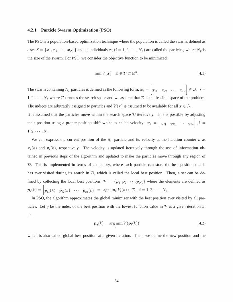
4.2.1 Particle Swarm Optimization (PSO)
The PSO is a population-based optimization technique wherethe population is called the swarm, defined as
a setS = x1,x2, · · · ,xNp and its individualsxi (i = 1, 2, · · · , Np) are called the particles, whereNp is
the size of the swarm. For PSO, we consider the objective function to be minimized:
minxV (x), x ∈ D ⊂ R
n. (4.1)
The swarm containingNp particles is defined as the following form:xi =
[
xi1 xi2 · · · xin
]
∈ D, i =
1, 2, · · · , Np whereD denotes the search space and we assume thatD is the feasible space of the problem.
The indices are arbitrarily assigned to particles andV (x) is assumed to be available for allx ∈ D.
It is assumed that the particles move within the search spaceD iteratively. This is possible by adjusting
their position using a proper position shift which is calledvelocity: vi =
[
vi1 vi2 · · · vin
]
, i =
1, 2, · · · , Np.
We can express the current position of theith particle and its velocity at the iteration counterk as
xi(k) and vi(k), respectively. The velocity is updated iteratively through the use of information ob-
tained in previous steps of the algorithm and updated to makethe particles move through any region of
D. This is implemented in terms of a memory, where each particle can store the best position that it
has ever visited during its search inD, which is called the local best position. Then, a set can be de-
fined by collecting the local best positions,P = p1,p2, · · · ,pNp where the elements are defined as
pi(k) =
[
pi1(k) pi2(k) · · · pin(k)
]
= argmink Vi(k) ∈ D, i = 1, 2, · · · , Np.
In PSO, the algorithm approximates the global minimizer with the best position ever visited by all par-
ticles. Letg be the index of the best position with the lowest function value inP at a given iterationk,
i.e.,
pg(k) = argmini
V (pi(k)) (4.2)
which is also called global best position at a given iteration. Then, we define the new position and the
34
velocity by the following equations (Clerc and Kennedy, 2002):
xij(k + 1) = xij(k) + vij(k + 1),
vij(k + 1) = χ(
vij(k) + c1R1
(pij(k)− xij(k)
)+ c2R2
(pgj(k)− xij(k)
))
(4.3)
for all i = 1, 2, · · · , Np, j = 1, 2, · · · , n whereR1 andR2 denote random variables uniformly distributed
within [0, 1]; andc1 andc2 are thecognitiveandsocialparameter, respectively. The parameterχ is called
constriction coefficient. Among the ways to define the values ofχ, c1, andc2, Clerc and Kennedy (2002)
suggested the following formula:
χ =2
φ− 2 +√
φ2 − 4φ(4.4)
whereφ = c1+c2 > 4. Based on (4.4), the default parameter set of the constriction coefficient is as follows:
χ = 0.729, c1 = c2 = 2.05. (4.5)
At each iteration, the best positions are also updated afterthe update and evaluation of particles. Thus,
we can define the new best position ofxi at iterationk + 1 as
pi(k + 1) =
xi(k + 1), if V(xi(k + 1)
)≤ V
(pi(k)
),
pi(k), otherwise.(4.6)
4.2.2 Algorithm of AGT-PSO
In this part, we introduce the mechanism of AGT-PSO.
1. Initial Setup for PSO
There are several parameters to be set upa priori in order to run PSO:
n : dimension of the problem (i.e., the number of parameters tobe tuned in PSO)
N : swarm size (i.e., the number of particles)
35
kmax : the maximum number of iterations
tol : tolerance of the simulation
U : the vector of the upper bounds of the tuning parameters
L : the vector of the lower bounds of the tuning parameters
2. Initial Conditions
As mentioned in the previous section, the standard PSO usesU andL to generate initial conditions. How-
ever, it is not always necessary if good initial conditions or desired values of the tuning parameters are given.
For this condition, a special parameter is defined:
RI : determination of the random initialization of the parameters
If RI ← 1, AGT-PSO starts with random initial conditions of the tuning parameters. IfRI ← 0, on
the other hand, users can define the initial conditions by themselves. This condition can be used to evaluate
parameters which were tuned manually. In this case, a special function can be used to assign the user-defined
initial conditions:
x0 = TuningIC(condition) (4.7)
wherex0 denotes the new initial conditions of the tuning parameterswhich were given externally depending
on “condition.”
For the case ofRI ← 1, the random initial conditions are generated by using the following equation:
current_position(j, i) = rand×(U(j)− L(j)
)+ L(j) (4.8)
wherej = 1, 2, · · · , n andi = 1, 2, · · · , kmaxRI . The functionrand and the constantkmaxRI denote the
uniform random number generator in[0 1] and the maximum number of iterations for obtaining random
36

initial conditions, respectively.
3. Model Update
The tuning parameters can be directly applied to tuning systems. However, depending on the tuning systems,
system models such as a dynamic model, a filter system, etc. must be updated by using the latest information
of the tuning parameters. In this case, a special function isused:
[model parameters] = Model_Update(current_position(:, i), (other parameters)
)(4.9)
4. Evaluation of Performance Index (PI)
In optimization problems, defining performance indices (orcost functions) plays an important role. There-
fore, more sophisticated performance index is recommended. In other words, a performance indexV to be
minimized for a given system can be simply defined as follows:
V =1
2
m∑
i=1
e⊤i Wiei (4.10)
whereei is the error of the system to be minimized andm ≥ 1 is the number of errors to be considered.
Figure 4.1 shows the flowchart of the AGT-PSO.
Remark 6 The performance index in (4.10) is a simple form. If there arespecific performance requirements
such as rise time (tr), settling time (ts), and % overshoot (Mp), the performance index in (4.10) should be
modified.
4.3 Performance Evaluation
In this section, we evaluate the performance of AGT-PSO withtwo examples from industry.
37
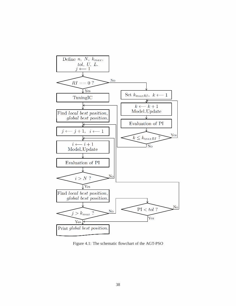
Figure 4.1: The schematic flowchart of the AGT-PSO
38
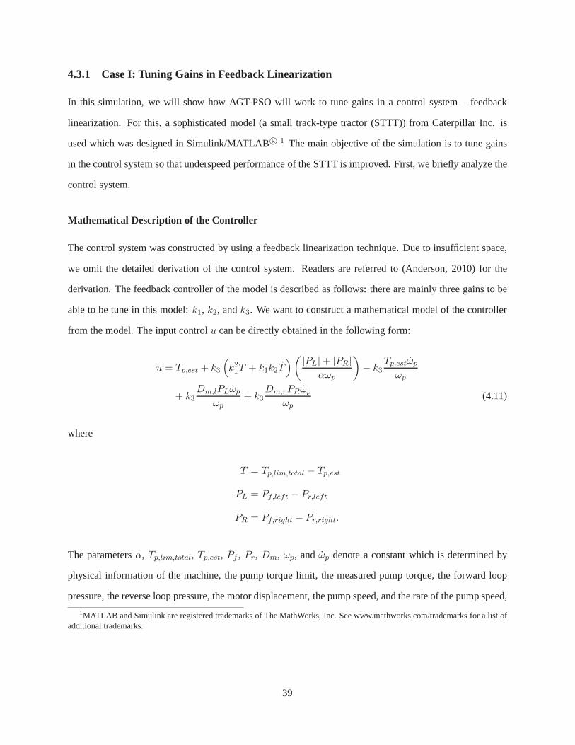
4.3.1 Case I: Tuning Gains in Feedback Linearization
In this simulation, we will show how AGT-PSO will work to tunegains in a control system – feedback
linearization. For this, a sophisticated model (a small track-type tractor (STTT)) from Caterpillar Inc. is
used which was designed in Simulink/MATLABR©.1 The main objective of the simulation is to tune gains
in the control system so that underspeed performance of the STTT is improved. First, we briefly analyze the
control system.
Mathematical Description of the Controller
The control system was constructed by using a feedback linearization technique. Due to insufficient space,
we omit the detailed derivation of the control system. Readers are referred to (Anderson, 2010) for the
derivation. The feedback controller of the model is described as follows: there are mainly three gains to be
able to be tune in this model:k1, k2, andk3. We want to construct a mathematical model of the controller
from the model. The input controlu can be directly obtained in the following form:
u = Tp,est + k3
(
k21T + k1k2T)( |PL|+ |PR|
αωp
)
− k3Tp,estωp
ωp
+ k3Dm,lPLωp
ωp+ k3
Dm,rPRωp
ωp(4.11)
where
T = Tp,lim,total − Tp,est
PL = Pf,left − Pr,left
PR = Pf,right − Pr,right.
The parametersα, Tp,lim,total, Tp,est, Pf , Pr, Dm, ωp, andωp denote a constant which is determined by
physical information of the machine, the pump torque limit,the measured pump torque, the forward loop
pressure, the reverse loop pressure, the motor displacement, the pump speed, and the rate of the pump speed,
1MATLAB and Simulink are registered trademarks of The MathWorks, Inc. See www.mathworks.com/trademarks for a list ofadditional trademarks.
39

respectively. The values ofk1, k2, andk3 were tuned manually and the values are set to
k1 = 43.9820
k2 = 1.6000 (4.12)
k3 = 0.0796.
By using the current gains, we want to evaluate the performance of the controlled system in the next sub-
section for future references.
Test of Simulation
In order to evaluate the performance of the controller (4.11) with the current gains (4.12) and that obtained
by using AGT-PSO, the model should be simulated under several conditions separately or simultaneously.
For the test, we designed a comprehensive test model shown inFigure 4.2(a). The simulation condition
comprises bank ram, forward-neutral-reverse (FNR) shifts, hill transition, and implement load. Notice that
the main objective of the control system here is to minimize the effort of the underspeed control action,
whose set point map can be found in Table 4.1.
Based on the mathematical description of the control system, we will obtain the optimal values ofk1, k2,
andk3 through the use of AGT-PSO in the following subsection.
Performance of AGT-PSO for Tuning the Gains
In this subsection, the performance of AGT-PSO will be evaluated with the STTT model. For this, we tested
two simulations with different assumptions: in the firs simulation, we assumed that the current gains (4.12)
are the starting point of the PSO. In the second simulation, on the other hand, it was assumed that we do not
know havea priori knowledge of the gains.
In the model, there are six variables (errors) to be considered: the torque error (T ), the rate of torque error
(T ), the motor speed errors (eωm,l(left) andeωm,r(right)), the engine speed error (ees), and the underspeed
error (eus) which are defined as:
40
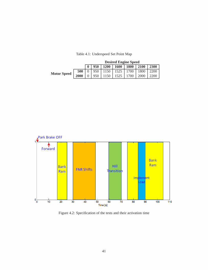
Table 4.1: Underspeed Set Point Map
Desired Engine Speed0 950 1200 1600 1800 2100 2300
Motor Speed500 0 950 1150 1525 1700 1800 2200
2000 0 950 1150 1525 1700 2000 2200
Figure 4.2: Specification of the tests and their activation time
41
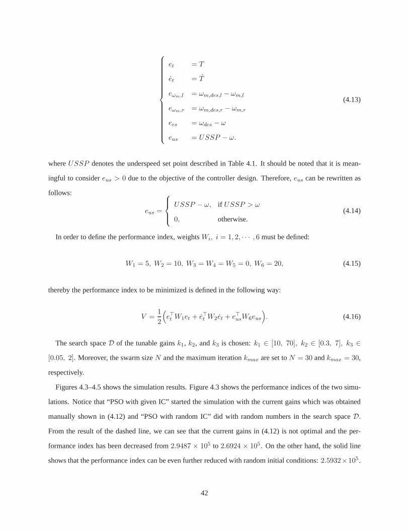
et = T
et = T
eωm,l = ωm,des,l − ωm,l
eωm,r = ωm,des,r − ωm,r
ees = ωdes − ω
eus = USSP − ω.
(4.13)
whereUSSP denotes the underspeed set point described in Table 4.1. It should be noted that it is mean-
ingful to considereus > 0 due to the objective of the controller design. Therefore,eus can be rewritten as
follows:
eus =
USSP − ω, if USSP > ω
0, otherwise.(4.14)
In order to define the performance index, weightsWi, i = 1, 2, · · · , 6 must be defined:
W1 = 5, W2 = 10, W3 =W4 =W5 = 0, W6 = 20, (4.15)
thereby the performance index to be minimized is defined in the following way:
V =1
2
(
e⊤t W1et + e⊤t W2et + e⊤usW6eus
)
. (4.16)
The search spaceD of the tunable gainsk1, k2, andk3 is chosen:k1 ∈ [10, 70], k2 ∈ [0.3, 7], k3 ∈
[0.05, 2]. Moreover, the swarm sizeN and the maximum iterationkmax are set toN = 30 andkmax = 30,
respectively.
Figures 4.3–4.5 shows the simulation results. Figure 4.3 shows the performance indices of the two simu-
lations. Notice that “PSO with given IC” started the simulation with the current gains which was obtained
manually shown in (4.12) and “PSO with random IC” did with random numbers in the search spaceD.
From the result of the dashed line, we can see that the currentgains in (4.12) is not optimal and the per-
formance index has been decreased from2.9487 × 105 to 2.6924 × 10⁵. On the other hand, the solid line
shows that the performance index can be even further reducedwith random initial conditions:2.5932×10⁵ .
42
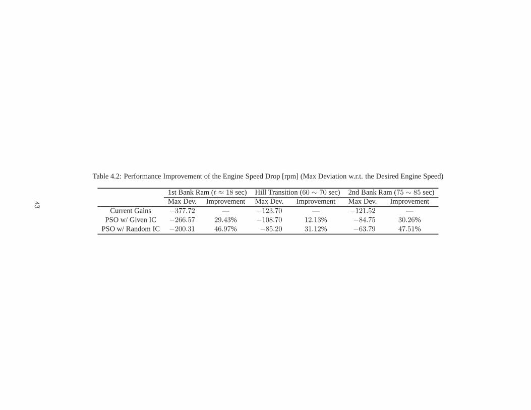
Table 4.2: Performance Improvement of the Engine Speed Drop[rpm] (Max Deviation w.r.t. the Desired Engine Speed)
1st Bank Ram (t ≈ 18 sec) Hill Transition (60 ∼ 70 sec) 2nd Bank Ram (75 ∼ 85 sec)Max Dev. Improvement Max Dev. Improvement Max Dev. Improvement
Current Gains −377.72 — −123.70 — −121.52 —PSO w/ Given IC −266.57 29.43% −108.70 12.13% −84.75 30.26%
PSO w/ Random IC −200.31 46.97% −85.20 31.12% −63.79 47.51%
43
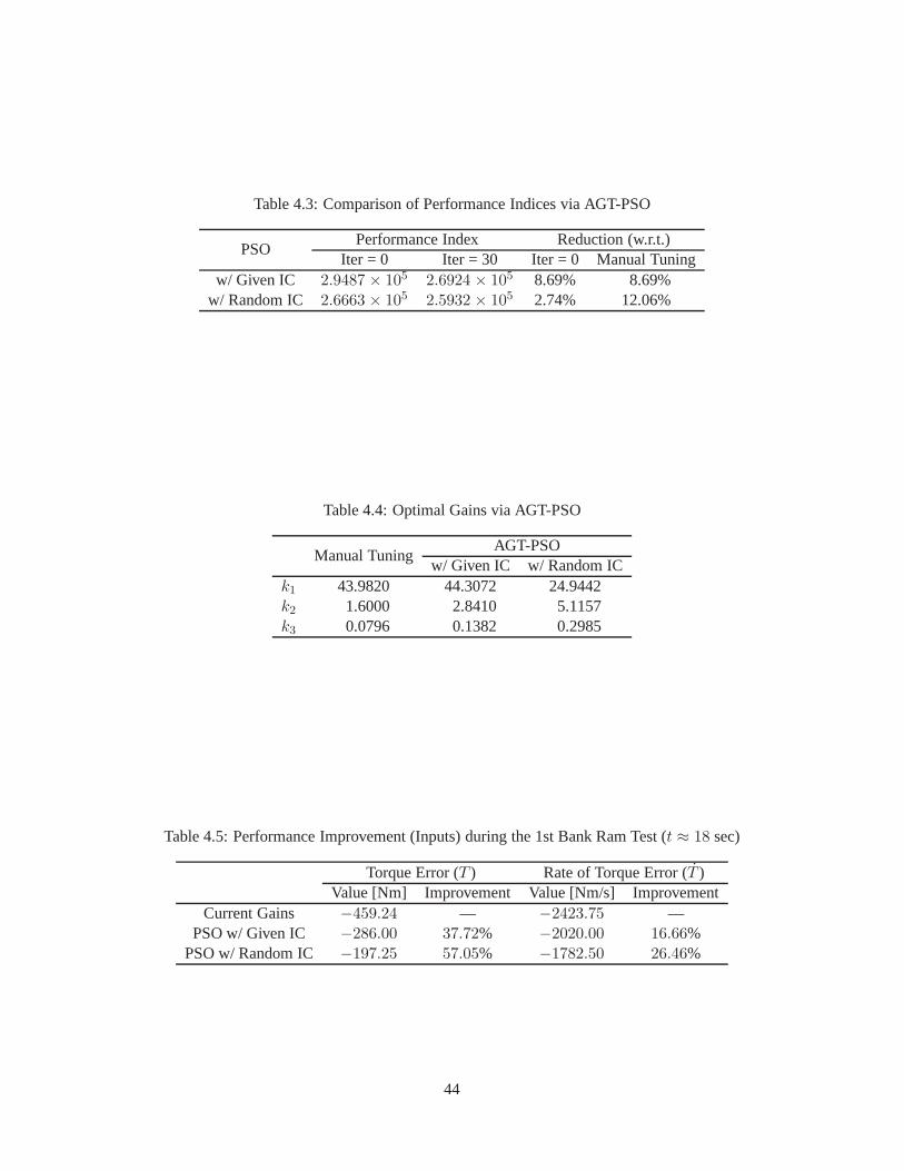
Table 4.3: Comparison of Performance Indices via AGT-PSO
PSOPerformance Index Reduction (w.r.t.)
Iter = 0 Iter = 30 Iter = 0 Manual Tuningw/ Given IC 2.9487 × 10⁵ 2.6924 × 10⁵ 8.69% 8.69%
w/ Random IC 2.6663 × 10⁵ 2.5932 × 10⁵ 2.74% 12.06%
Table 4.4: Optimal Gains via AGT-PSO
Manual TuningAGT-PSO
w/ Given IC w/ Random ICk1 43.9820 44.3072 24.9442k2 1.6000 2.8410 5.1157k3 0.0796 0.1382 0.2985
Table 4.5: Performance Improvement (Inputs) during the 1stBank Ram Test (t ≈ 18 sec)
Torque Error (T ) Rate of Torque Error (T )Value [Nm] Improvement Value [Nm/s] Improvement
Current Gains −459.24 — −2423.75 —PSO w/ Given IC −286.00 37.72% −2020.00 16.66%
PSO w/ Random IC −197.25 57.05% −1782.50 26.46%
44
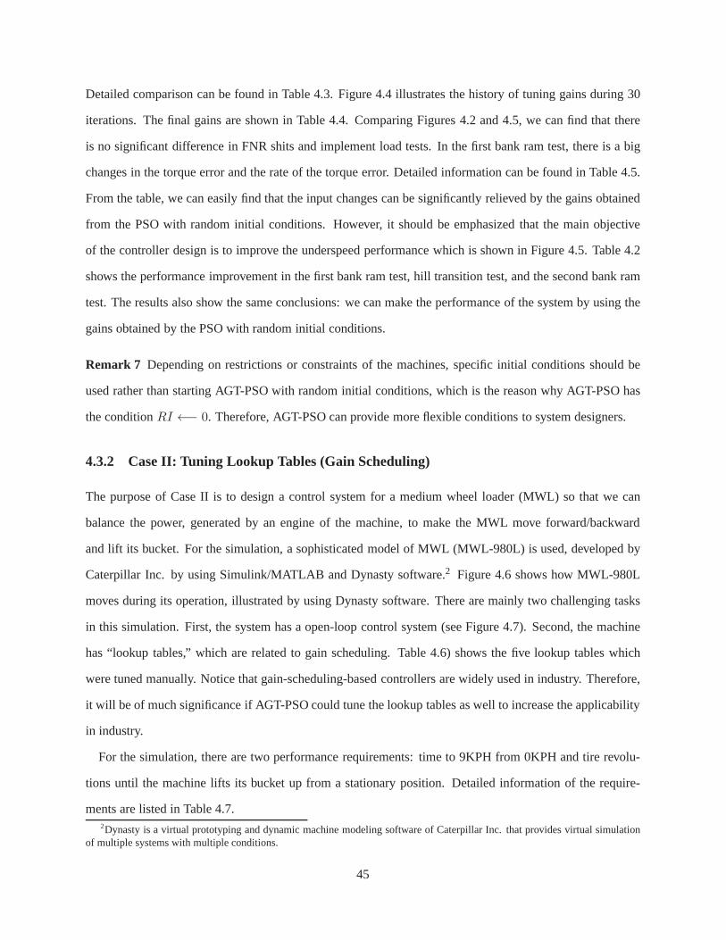
Detailed comparison can be found in Table 4.3. Figure 4.4 illustrates the history of tuning gains during 30
iterations. The final gains are shown in Table 4.4. ComparingFigures 4.2 and 4.5, we can find that there
is no significant difference in FNR shits and implement load tests. In the first bank ram test, there is a big
changes in the torque error and the rate of the torque error. Detailed information can be found in Table 4.5.
From the table, we can easily find that the input changes can besignificantly relieved by the gains obtained
from the PSO with random initial conditions. However, it should be emphasized that the main objective
of the controller design is to improve the underspeed performance which is shown in Figure 4.5. Table 4.2
shows the performance improvement in the first bank ram test,hill transition test, and the second bank ram
test. The results also show the same conclusions: we can makethe performance of the system by using the
gains obtained by the PSO with random initial conditions.
Remark 7 Depending on restrictions or constraints of the machines, specific initial conditions should be
used rather than starting AGT-PSO with random initial conditions, which is the reason why AGT-PSO has
the conditionRI ←− 0. Therefore, AGT-PSO can provide more flexible conditions tosystem designers.
4.3.2 Case II: Tuning Lookup Tables (Gain Scheduling)
The purpose of Case II is to design a control system for a medium wheel loader (MWL) so that we can
balance the power, generated by an engine of the machine, to make the MWL move forward/backward
and lift its bucket. For the simulation, a sophisticated model of MWL (MWL-980L) is used, developed by
Caterpillar Inc. by using Simulink/MATLAB and Dynasty software.2 Figure 4.6 shows how MWL-980L
moves during its operation, illustrated by using Dynasty software. There are mainly two challenging tasks
in this simulation. First, the system has a open-loop control system (see Figure 4.7). Second, the machine
has “lookup tables,” which are related to gain scheduling. Table 4.6) shows the five lookup tables which
were tuned manually. Notice that gain-scheduling-based controllers are widely used in industry. Therefore,
it will be of much significance if AGT-PSO could tune the lookup tables as well to increase the applicability
in industry.
For the simulation, there are two performance requirements: time to 9KPH from 0KPH and tire revolu-
tions until the machine lifts its bucket up from a stationaryposition. Detailed information of the require-
ments are listed in Table 4.7.2Dynasty is a virtual prototyping and dynamic machine modeling software of Caterpillar Inc. that provides virtual simulation
of multiple systems with multiple conditions.
45
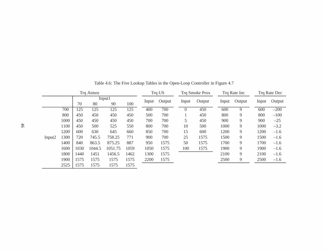
Table 4.6: The Five Lookup Tables in the Open-Loop Controller in Figure 4.7
Trq Atmos Trq US Trq Smoke Prox Trq Rate Inc Trq Rate DecInput1
Input Output Input Output Input Output Input Output70 80 90 100
Input2
700 125 125 125 125 400 700 0 450 600 9 600 –200800 450 450 450 450 500 700 1 450 800 9 800 –1001000 450 450 450 450 700 700 5 450 900 9 900 –251100 450 500 525 550 800 700 10 500 1000 9 1000 –3.21200 600 630 645 660 850 700 15 600 1200 9 1200 –1.61300 720 745.5 758.25 771 900 700 25 1575 1500 9 1500 –1.61400 840 863.5 875.25 887 950 1575 50 1575 1700 9 1700 –1.61600 1030 1044.5 1051.75 1059 1050 1575 100 1575 1900 9 1900 –1.61800 1440 1451 1456.5 1462 1300 1575 2100 9 2100 –1.61900 1575 1575 1575 1575 2200 1575 2500 9 2500 –1.62525 1575 1575 1575 1575
46
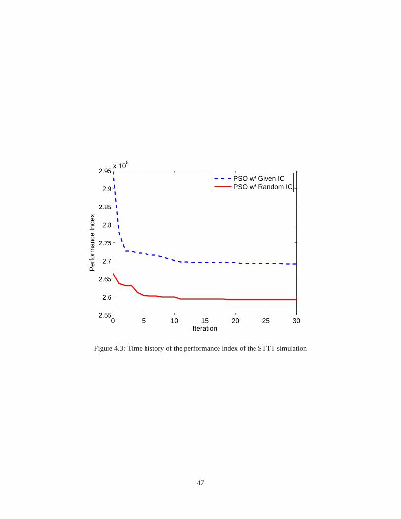
0 5 10 15 20 25 302.55
2.6
2.65
2.7
2.75
2.8
2.85
2.9
2.95x 10
5
Iteration
Per
form
ance
Inde
x
PSO w/ Given ICPSO w/ Random IC
Figure 4.3: Time history of the performance index of the STTTsimulation
47
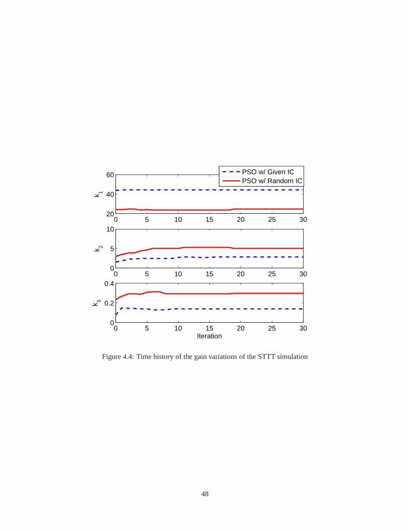
0 5 10 15 20 25 3020
40
60
k 1
0 5 10 15 20 25 300
5
10
k 2
0 5 10 15 20 25 300
0.2
0.4
Iteration
k 3
PSO w/ Given ICPSO w/ Random IC
Figure 4.4: Time history of the gain variations of the STTT simulation
48
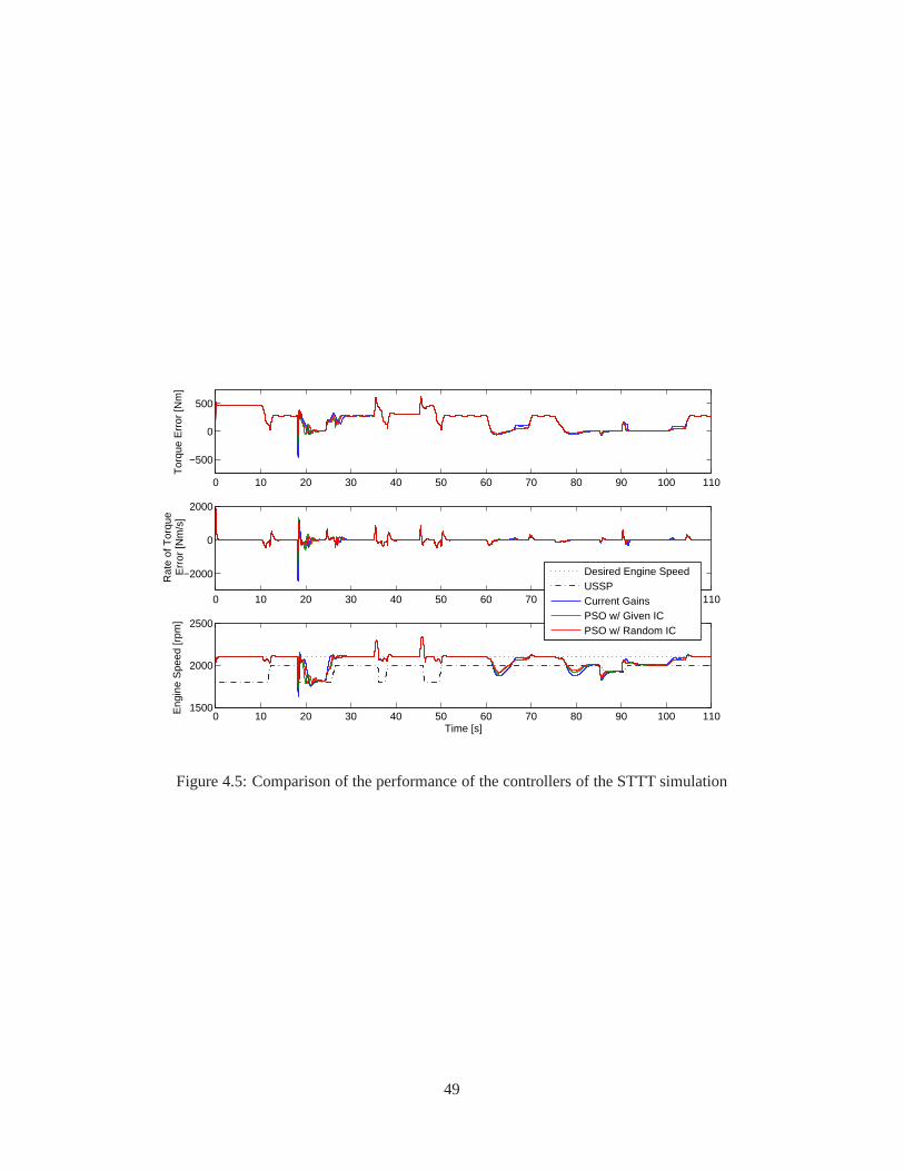
0 10 20 30 40 50 60 70 80 90 100 110
−500
0
500
Tor
que
Err
or [N
m]
0 10 20 30 40 50 60 70 80 90 100 110
−2000
0
2000
Rat
e of
Tor
que
Err
or [N
m/s
]
0 10 20 30 40 50 60 70 80 90 100 1101500
2000
2500
Time [s]
Eng
ine
Spe
ed [r
pm]
Desired Engine SpeedUSSPCurrent GainsPSO w/ Given ICPSO w/ Random IC
Figure 4.5: Comparison of the performance of the controllers of the STTT simulation
49
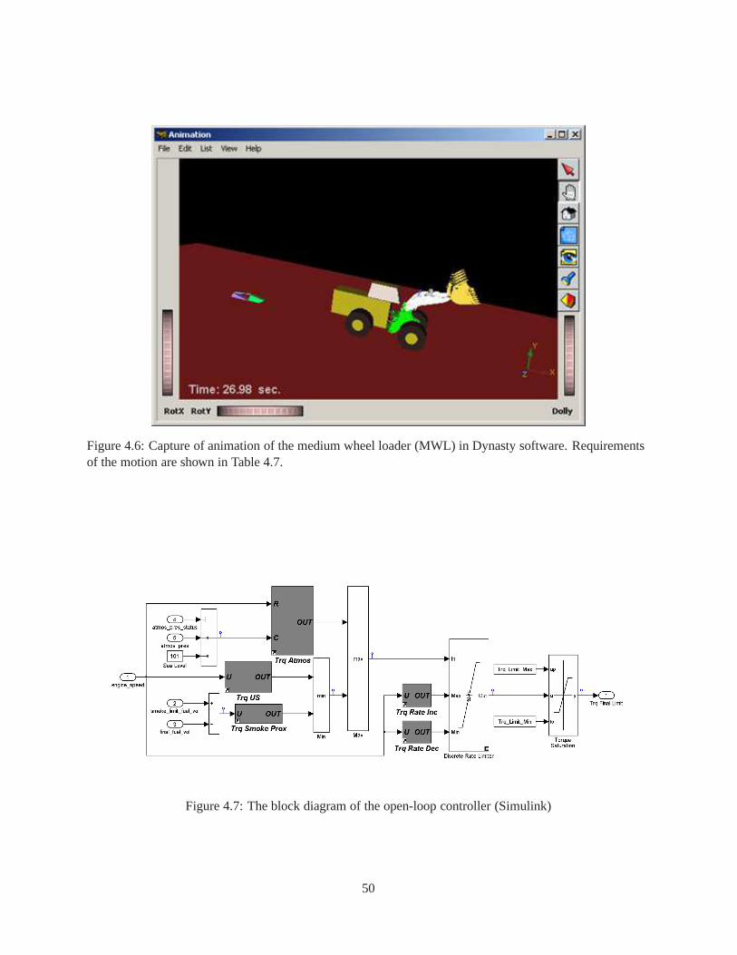
Figure 4.6: Capture of animation of the medium wheel loader (MWL) in Dynasty software. Requirementsof the motion are shown in Table 4.7.
Figure 4.7: The block diagram of the open-loop controller (Simulink)
50
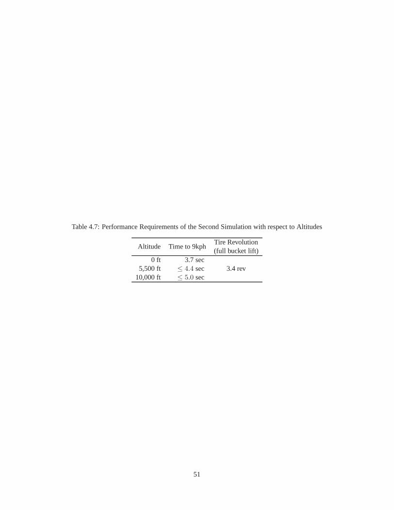
Table 4.7: Performance Requirements of the Second Simulation with respect to Altitudes
Altitude Time to 9kphTire Revolution(full bucket lift)
0 ft 3.7 sec5,500 ft ≤ 4.4 sec 3.4 rev
10,000 ft ≤ 5.0 sec
51
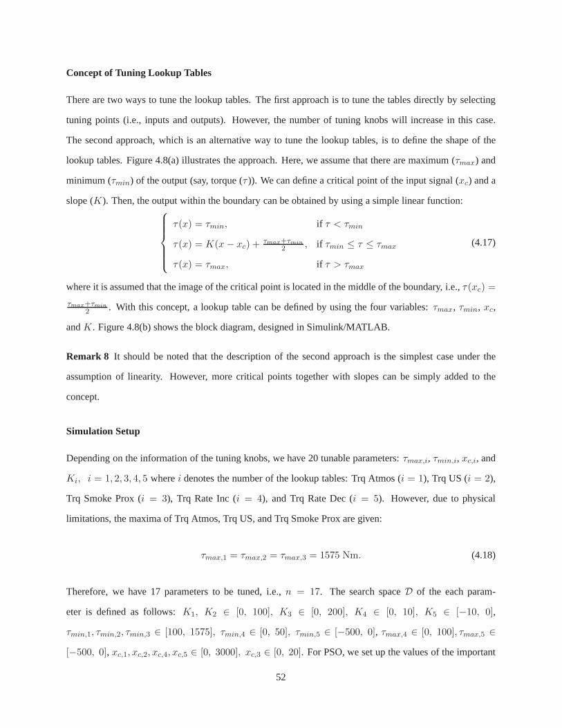
Concept of Tuning Lookup Tables
There are two ways to tune the lookup tables. The first approach is to tune the tables directly by selecting
tuning points (i.e., inputs and outputs). However, the number of tuning knobs will increase in this case.
The second approach, which is an alternative way to tune the lookup tables, is to define the shape of the
lookup tables. Figure 4.8(a) illustrates the approach. Here, we assume that there are maximum (τmax) and
minimum (τmin) of the output (say, torque (τ )). We can define a critical point of the input signal (xc) and a
slope (K). Then, the output within the boundary can be obtained by using a simple linear function:
τ(x) = τmin, if τ < τmin
τ(x) = K(x− xc) + τmax+τmin
2 , if τmin ≤ τ ≤ τmax
τ(x) = τmax, if τ > τmax
(4.17)
where it is assumed that the image of the critical point is located in the middle of the boundary, i.e.,τ(xc) =
τmax+τmin
2 . With this concept, a lookup table can be defined by using the four variables:τmax, τmin, xc,
andK. Figure 4.8(b) shows the block diagram, designed in Simulink/MATLAB.
Remark 8 It should be noted that the description of the second approach is the simplest case under the
assumption of linearity. However, more critical points together with slopes can be simply added to the
concept.
Simulation Setup
Depending on the information of the tuning knobs, we have 20 tunable parameters:τmax,i, τmin,i, xc,i, and
Ki, i = 1, 2, 3, 4, 5 wherei denotes the number of the lookup tables: Trq Atmos (i = 1), Trq US (i = 2),
Trq Smoke Prox (i = 3), Trq Rate Inc (i = 4), and Trq Rate Dec (i = 5). However, due to physical
limitations, the maxima of Trq Atmos, Trq US, and Trq Smoke Prox are given:
τmax,1 = τmax,2 = τmax,3 = 1575 Nm. (4.18)
Therefore, we have 17 parameters to be tuned, i.e.,n = 17. The search spaceD of the each param-
eter is defined as follows:K1, K2 ∈ [0, 100], K3 ∈ [0, 200], K4 ∈ [0, 10], K5 ∈ [−10, 0],
τmin,1, τmin,2, τmin,3 ∈ [100, 1575], τmin,4 ∈ [0, 50], τmin,5 ∈ [−500, 0], τmax,4 ∈ [0, 100], τmax,5 ∈
[−500, 0], xc,1, xc,2, xc,4, xc,5 ∈ [0, 3000], xc,3 ∈ [0, 20]. For PSO, we set up the values of the important
52

(a) Concept of defining a lookup table
(b) Implementation of the concept in Simulink/MATLAB
Figure 4.8: Alternative approach to tune the lookup tables
53

parameters:N = 40, kmax = 40, tol = 10−5. Moreover, it is assumed that we do not have good initial
conditions of the parameters, i.e.,RI ←− 1.
The performance index in this problem is constructed with two performance criteria:e9KPH andetire,
thereby it has the following form:
V =1
2
(
e⊤9KPHW1e9KPH + e⊤tireW2etire
)
(4.19)
wheree9KPH denotes the normalized time error to 9KPH (i.e.,e9KPH := (t − 3.7 − 20)/3.7 for altitude =
0 ft)3 andetire is the normalized tire revolution error (i.e.,etire := (rev − 3.4)/3.4).
Performance of AGT-PSO for Tuning the Lookup Tables
There are different performance requirements depending onthe altitudes. Since the results are similar, we
will show the results at the sea level (altitude = 0 ft). The history of the performance index is shown in
Figure 4.9. Notice that the simulation was terminated atj = 18 since the value of the performance index
(5.5826 × 10⁻⁶) was lower thantol = 10−5. The new five lookup tables are plotted4 in Figure 4.10. The
shape of the new lookup tables (solid lines) are different from the original ones in the sense that they have
different slopes (Ki) and critical points (xc,i) in most cases. The performance of the machine can be found in
Figure 4.11. As can be seen from the two figures, the results bythe new lookup tables meet the performance
requirements in Table 4.7 while those by the original lookuptables failed to satisfy the requirements.
Remark 9 AGT-PSO not only provides optimal values of the parameters to be tuned, but it also shows
meaningful results within a relatively short time while themanual tuning hardly does it as can be seen from
the two simulation tests.
4.4 Conclusions
In this chapter, we introduced an automatic gain-tuner via particle swarm optimization. The suggested gain
tuning system through the use of PSO has shown to be beneficiary in the sense that the obtained control
gains are guaranteed to beoptimal or suboptimal. Moreover, the performance of the controlled system
3The machine starts to move from 20 sec.4For the simple comparison of the original lookup tables and new ones, obtained by using AGT-PSO, we plotted them instead
of showing them in the form of tables such as Table 4.6.
54
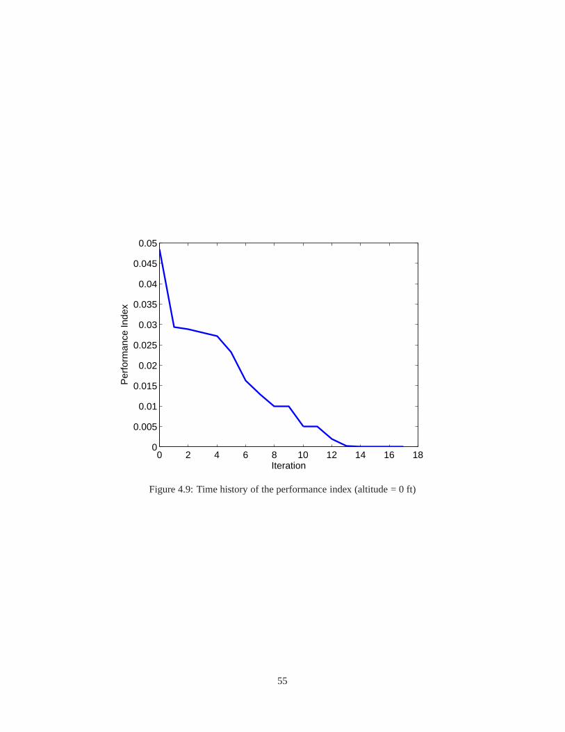
0 2 4 6 8 10 12 14 16 180
0.005
0.01
0.015
0.02
0.025
0.03
0.035
0.04
0.045
0.05
Iteration
Per
form
ance
Inde
x
Figure 4.9: Time history of the performance index (altitude= 0 ft)
55
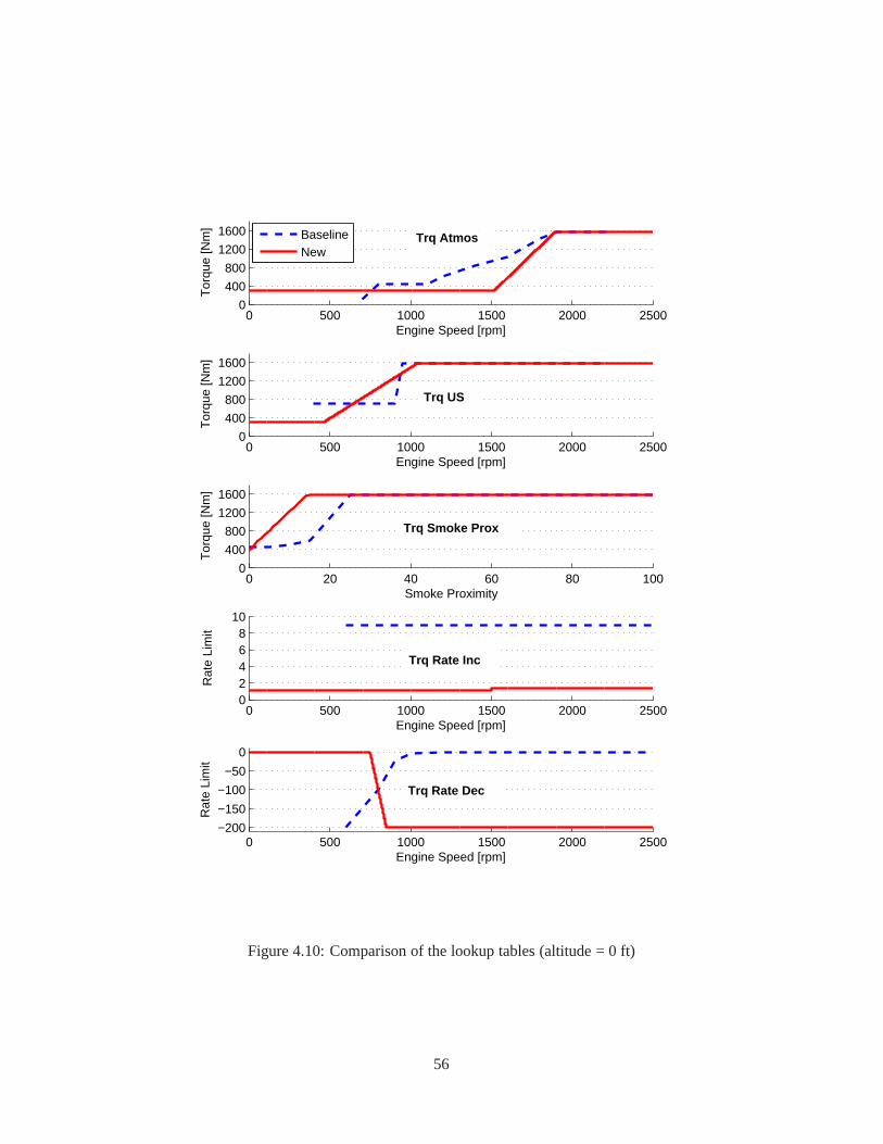
0 500 1000 1500 2000 25000
400
800
1200
1600
Engine Speed [rpm]
Tor
que
[Nm
]
0 500 1000 1500 2000 25000
400
800
1200
1600
Engine Speed [rpm]
Tor
que
[Nm
]
0 20 40 60 80 1000
400
800
1200
1600
Smoke Proximity
Tor
que
[Nm
]
0 500 1000 1500 2000 250002468
10
Engine Speed [rpm]
Rat
e Li
mit
0 500 1000 1500 2000 2500−200
−150
−100
−50
0
Engine Speed [rpm]
Rat
e Li
mit
BaselineNew
Trq US
Trq Atmos
Trq Rate Inc
Trq Rate Dec
Trq Smoke Prox
Figure 4.10: Comparison of the lookup tables (altitude = 0 ft)
56
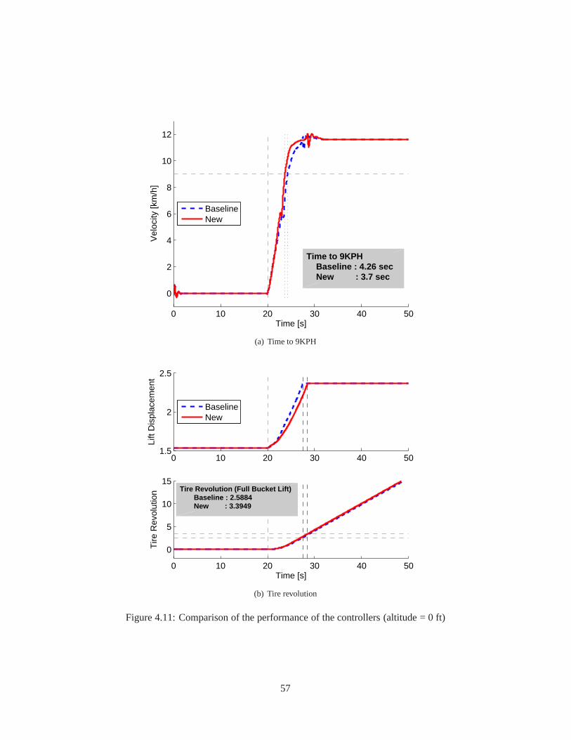
0 10 20 30 40 50
0
2
4
6
8
10
12
Time [s]
Vel
ocity
[km
/h]
BaselineNew
Time to 9KPH Baseline : 4.26 sec New : 3.7 sec
(a) Time to 9KPH
0 10 20 30 40 501.5
2
2.5
Lift
Dis
plac
emen
t
0 10 20 30 40 50
0
5
10
15
Time [s]
Tire
Rev
olut
ion
BaselineNew
Tire Revolution (Full Bucket Lift) Baseline : 2.5884 New : 3.3949
(b) Tire revolution
Figure 4.11: Comparison of the performance of the controllers (altitude = 0 ft)
57

could be modified by the designers’ choice of the weights in the performance index. The main advantage
of the automatic gain-tuners lies in the fact that it does notrequire any specific information to use it which
in turn skills of the well-experienced control engineers can be easily replaed by the to tune parameters of
the machines. AGT-PSO also provides the choice to start it with random initial conditions of the tunable
parameters or meaningful initial conditions givena priori. It should be emphasized that AGT-PSO will
significantly reduce time and labor to tune system parameters.
58
Part II
Constrained Discrete-Time
State-Dependent Riccati Equation
Technique
59
Chapter 5
Constrained Discrete-TimeState-Dependent Riccati EquationTechnique
THE objective of this chapter is to introduce the discrete-timestate-dependent Riccati equation tech-
nique under input and state constraints, yielding constrained (C) discrete-time (D) SDRE, referred to
as CD-SDRE. For the latter, stability analysis and calculation of a region of attraction are carried out. The
derivation of the D-SDRE under state-dependent weights is provided. Stability of the D-SDRE feedback
system is established using the Lyapunov stability approach. Receding horizon strategy is used to take into
account the constraints on D-SDRE controller. Stability condition of the CD-SDRE controller is analyzed
by using a switched system.
This chapter is organized as follows: In the following section, the derivation of D-SDRE, its stability
condition, and estimates of a region of attraction of the D-SDRE feedback system are presented. The CD-
SDRE is established in Section 5.2. Finally, concluding remarks are made in Section 5.3.
5.1 Generalized Discrete-Time State-Dependent Riccati Equation
(D-SDRE) Technique
In this section, we derive the D-SDRE by using the optimalitycondition through the use of the Hamiltonian.
Then, stability conditions of the D-SDRE feedback system are provided via the Lyapunov stability analysis.
An ROA of a nonlinear system controlled by the D-SDRE feedback controller is investigated subsequently.
5.1.1 Derivation of the D-SDRE Feedback Controller
Consider the discrete-time nonlinear control-affine system described by using the nonlinear difference equa-
tion
xk+1 = f(xk) +B(xk)uk k ∈ Z≥0 (5.1)
60
wherexk ∈ X ⊆ Rn anduk ∈ U ⊆ R
m. It is assumed thatf(0) = 0 andf(xk) is continuously
differentiable. In this case, the model can be rearranged through the use of the SDC factorization (Cloutier,
1997):
xk+1 = A(xk)xk +B(xk)uk. (5.2)
We assume that(A(xk),B(xk)) is piecewise controllable for allxk ∈ X. For this system, the D-SDRE
technique finds a control inputuk ∈ U at each time that approximately minimizes the following perfor-
mance index:
J0 =1
2
k+N−1∑
j=k
(
x⊤j Q(xj)xj + u⊤
j R(xj)uj
)
(5.3)
where the weightsQ(xj) andR(xj), which are assumed to be differentiable atxk for all k ∈ Z≥0, are
symmetric positive semi-definite and symmetric positive definite, respectively.
To find the optimal feedback controlleru(xk), the Hamiltonian defined as below is used:
Hk =1
2
(
x⊤k Q(xk)xk + u⊤
k R(xk)uk
)
+ λ⊤k+1
(
f(xk) +B(xk)uk
)
. (5.4)
Applying the optimality condition (Kirk, 1970; Bryson, Jr.and Ho, 1975), we obtain the three equations:
State equation
xk+1 =∂Hk
∂λk+1= f(xk) +B(xk)uk (5.5)
Costate equation
λk =∂Hk
∂xk= Q+ A
⊤λk+1 (5.6)
Stationary condition
0 =∂Hk
∂uk= B(xk)
⊤λk+1 +R(xk)uk (5.7)
whereQ := Q(xk)xk +12x
⊤k
∂Q(xk)∂xk
xk +12u
⊤k
∂R(xk)∂xk
uk andA := A(xk) +∂A(xk)∂xk
xk +∂B(xk)∂xk
uk.
To find the optimal solution, it is assumed that
λk = P kxk. (5.8)
61
Substituting (5.8) into (5.7) yields
u(xk) = −R(xk)−1B(xk)
⊤λk+1
= −R(xk)−1B(xk)
⊤P k+1 (A(xk)xk +B(xk)uk)
⇒ u(xk) = −(
R(xk) +B(xk)⊤P k+1B(xk)
)−1B(xk)
⊤
× P k+1A(xk)xk =: −K(xk)xk (5.9)
whereK(xk) ∈ Rm×n is the optimal feedback control gain of the D-SDRE technique.
It should be noted that in order to obtainK(xk), P k andP k+1 are needed, which are the solutions of the
generalized discrete-time Riccati equation (GD-RE) at timesk andk + 1, respectively. Substituting (5.8),
(5.5), and (5.9) into (5.6) and applying the matrix inversion lemma (Lewis et al., 2012) yield the following
derivation:
P kxk = Q+ A⊤λk+1
= Q+ A⊤P k+1xk+1
= Q+ A⊤P k+1 (A(xk)xk +B(xk)uk)
= Q+ A⊤P k+1
(
A(xk)xk −B(xk)(
R(xk) +B⊤(xk)P k+1B(xk))−1
B⊤(xk)P k+1A(xk)xk
)
= Q+ A⊤P k+1
(
I −B(xk)(
R(xk) +B⊤(xk)P k+1B(xk))−1
B⊤(xk)P k+1
)
A(xk)xk
= Q+ A⊤P k+1
(
I +B(xk)R−1(xk)B
⊤(xk)P k+1
)−1A(xk)xk.
Therefore, the GD-RE is obtained:
P k =
(
Q(xk) +1
2x⊤k
∂Q(xk)
∂xk− 1
2u⊤k
∂R(xk)
∂xkK(xk)
)
+ A⊤P k+1
(
I +B(xk)R(xk)−1B(xk)
⊤P k+1
)−1A(xk). (5.10)
Remark 10 The algebraic Riccati equation (ARE) is used in LQR problems. In (Cloutier, 1997) and many
other studies on SDRE, the ARE has been commonly used. Likewise, the DARE in (2.5) can be used
for D-SDRE (Algorithm 1 in (Dutka et al., 2005)). In this case, there is an assumption thatA(xk) =
62

∂∂xk
(f(xk) +B(xk)uk) ∀xk ∈ X. However, it is not satisfied in general. Therefore, the feedback
controlleruk may not work properly in an optimal sense unless∂A(xk)∂xk
xk +∂B(xk)∂xk
uk = 0 ∀xk ∈ X.
Remark 11 In this chapter,Q andR in (5.3) are assumed to be dependent on the statexk, i.e.,Q = Q(xk)
andR = R(xk). For simplicity,Q andR can be considered to be independent onxk. Then,Q = Q in
(5.6), and (5.10) becomes the same formula as that in Algorithm 2 in (Dutka et al., 2005). However, since
Q andR affect the performance of an optimal control problem such asD-SDRE, it is more desirable to use
state-dependent matrices rather than constant ones.
5.1.2 Stability Analysis of D-SDRE
It should be noted that the D-SDRE feedback controller is stabilizing the discrete-time nonlinear difference
equation (5.1) or (5.2). In this part, we investigate the stability of the D-SDRE controller. Prior to that, we
introduce exponential stability conditions.
Definition 6 Consider the discrete-time nonlinear system
ξk+1 = f(ξ,µ). (5.11)
Let (5.11) be a locally Lipschitz function inX ⊆ Rn andV : Rn → R≥0 be a continuously differentiable
function. Then (5.11) is said to be exponentially stable inX andV is called a Lyapunov function for (5.11)
if the following hold:
1. There existα1, α2 ∈ K∞ such that
α1(|ξ|) ≤ V (ξ) ≤ α2(|ξ|) ∀ξ ∈ Rn. (5.12)
2. There existsα3 ∈ K∞ such that
V (f(ξ,µ))− V (ξ) ≤ −α3(|ξ|) ∀ ξ ∈ Rn. (5.13)
Theorem 7 The discrete-time nonlinear system (5.2) controlled by theD-SDRE technique (5.9) is exponen-
tially stable in the ROA of the systemX ⊂ X.
63

Proof By substituting (5.9) into (5.2), we obtain the closed-loopform of the system:
xk+1 =
A(xk)−B(xk)(
R(xk) +B(xk)⊤P k+1B(xk)
)−1
×B(xk)⊤P k+1A(xk)
xk =: Acl(xk)xk. (5.14)
Then, we can derive the following equation by using the direct substitution into (5.14):
xk+1 =
k∏
j=0
Acl(xj)x0. (5.15)
By assumption in (5.2),(A(xk), B(xk)) is piecewise controllable forxk ∈ X, which implies that the
system is stabilizable. Then, forζ < 1, there existc > 0 and0 ≤ σ < ζ such that
‖Acl(xk)‖ ≤ cσk ≤ cσmax (5.16)
whereσmax = maxk σk.
We need to find a Lyapunov function of (5.2). GivenD = D⊤ > 0, we can findMk = M⊤k > 0 for
eachk from the following equation:
A⊤cl(xk)MkAcl(xk)−Mk−1 = −D. (5.17)
Consider the following Lyapunov function candidate:
V (xk) = x⊤k Mk−1xk. (5.18)
It shows thatV (xk) ≥ λmin|xk|2 =: α1(|xk|) andV (xk) ≤ λmax|xk|2 =: α2(|xk|) where
λmin = mink λmin(M k)
λmax = maxk λmax(M k).(5.19)
64
Then, we can findα3(|xk|) in Definition 6 from (5.2), (5.14)–(5.19):
V (xk+1)− V (xk) = x⊤k+1M kxk+1 − x⊤
k Mk−1xk
= x⊤k A
⊤clMkAclx
⊤k − x⊤
k Mk−1xk
= −x⊤k Dxk ≤ −λmin(D)|xk|2 =: −α3(|xk|), (5.20)
which implies thatV in (5.18) is a Lyapunov function and therefore, the system (5.2) controlled by (5.9) is
exponentially stable in its ROA.
5.1.3 Estimates of Region of Attraction (ROA) of D-SDRE
We consider a discrete-time nonlinear system controlled bythe D-SDRE technique. We have shown that
given the nonlinear system (5.1), under the assumption of anautonomous nonlinear equation, it can be
rewritten in the form of (5.2) by using the SDC factorization. Moreover, by (5.9), the closed-loop system
controlled by the D-SDRE feedback controller was obtained in (5.14). However, it should be emphasized
that it is difficult to expressAcl(xk) in an analytic form due to the difficulty of an analytic expression of
P k andP k+1. Therefore, we should approach the problem in a different way: one can view this problem
as a robust stability problem by assuming thatAcl(xk) is not precisely known, but it stays inG, a convex,
closed, and bounded domain (polytope) (Ramos and Peres, 2001), i.e.,
G =
Acl(α) : Acl(α) =
L∑
i=1
αiAcl,i;
L∑
i=1
αi = 1; αi ≥ 0
(5.21)
whereAcl,i are the vertices of the polytopeG.
Then, we have useful lemmas to find the ROA of the D-SDRE feedback system.
Lemma 8 SupposeAcl(xk) has uncertainties but belongs toG in (5.21). Then, (5.14) is robustly stable in
G if there existsP = P⊤ > 0 such that
A⊤cl,iPAcl,i −P < −ρI (5.22)
for all i = 1, 2, · · · , L andρ > 0.
65
Proof See (de Oliveira et al., 1999; Jiang and Wang, 2001). .
Lemma 9 SupposeAcl(xk) has uncertainties but belongs toG in (5.21). Then, (5.14) is robustly stable in
G if there existP i = P⊤i > 0 andG such that
P i A⊤cl,iG
⊤
GAcl,i G+G⊤ −P i
> ρI (5.23)
for all i = 1, 2, · · · , L andρ > 0.
Proof See (de Oliveira et al., 1999). .
Note that Lemmas 8 and 9 can be easily established by standardLMI solvers sinceAcl,i, the vertices of
the polytopeG, are linear and so is (5.23) onP i. Therefore, the ROA of D-SDRE feedback control system,
X ⊆ X ⊆ X ⊆ Rn can be obtained by the following way:
X =
x ∈ X : Acl(x) ∈ G in (5.21)
. (5.24)
.
So far, we derived the D-SDRE feedback controller and provedthe stability condition in an ROA which
is obtained numerically via LMIs. Notice that we assumed that there are no constraints on the states or the
control inputs. In order for the proposed control technique(CD-SDRE) to handle such constraints, MPC is
used. In the next section, we discuss MPC, its stability condition, and finally CD-SDRE.
5.2 Constrained Discrete-Time State-Dependent Riccati Equation
(CD-SDRE) Technique
In this section, we consider the D-SDRE technique with constraints on the statesxk and the control inputs
uk. As a second part of the proposed CD-SDRE, MPC is presented. Stability analysis of the CD-SDRE is
investigated subsequently. Finally, algorithms of CD-SDRE for regulation / tracking problems are provided.
66
5.2.1 Stability Analysis of MPC Mode
The proposed CD-SDRE uses MPC for two purposes: 1) to give directions to D-SDRE (guidance) by
providing values of the parameters such asP i in (5.10) and 2) to handle constraints onxk oruk. Therefore,
the proposed controller can be viewed as a hybrid system withtwo different controllers with a proper
activation mode. We already showed the stability conditionof the D-SDRE controller. We need to show
that of the MPC controller.
Given a discrete-time nonlinear control-affine system (5.2), we want to find an optimal control sequence:
µN (xk, k) := µk(xk, k), µk+1(xk, k), · · · , µk+N−1(xk, k) (5.25)
that minimizes the following performance index
JN (xk) =k+N−1∑
i=k
(
x⊤i Q(xi)xi + u⊤
i R(xi)ui
)
+ x⊤k+NS(xk+N )xk+N (5.26)
subject to (5.2),xk ∈ X, anduk ∈ U whereX is convex and closed inRn andU is convex and compact in
Rm both of which contain their origins.
An optimization technique such as dynamic program discussed in (Rawlings and Mayne, 2009) or PSO
discussed in Chapter 4 can yield an optimal control sequenceµN (xk, k). Then the optimal controlled
system satisfies
xk+1 = A(xk)xk +B(xk)uk (5.27)
whereuk := µk(xk, k) in (5.25).
For the stability proof of the system controlled by MPC, we need assumptions as follows.
Assumption 10 The stage cost and the terminal cost satisfy the bound conditions
∑k+N−1i=k x⊤
i Q(xi)xi + u⊤i R(xi)ui ≥ α1(|xk|)
x⊤k+NS(xk+N)xk+N ≤ α2(|xk|)
∀xk ∈ XN , ∀uk ∈ U whereα1(·), α2(·) ∈ K∞ andXN ∈ X is a region of attraction of the system
controlled by MPC.
67
Assumption 11 The following inequality holds for allk ∈ Z≥0:
minu∈U
k+N−1∑
i=k
x⊤i Q(xi)xi + u⊤
i R(xi)ui + x⊤k+NS(xk+N )xk+N ≤ x⊤
k+N−1S(xk+N−1)xk+N−1.
By means of the assumptions, we can prove the following theorem.
Theorem 12 Given the discrete-time nonlinear control-affine system in(5.2), the performance index in
(5.26), and the optimal control sequence (5.25), there exist α1(·), α2(·) ∈ K∞ such thatJN (·) satisfies the
following inequalities:
JN (xk) ≥ α1(|xk|) ∀xk ∈ XN
JN (xk) ≤ α2(|xk|) ∀xk ∈ XN
JN (xk+1)− JN (xk) ≤ −α1(|xk|) ∀xk ∈ XN .
(5.28)
Proof See Proposition 2.18 in (Rawlings and Mayne, 2009).
Theorem 12 shows that the system controlled by MPC is exponentially stable inXN . However, it should
be noted that the system is based on an open-loop control. Forrigorous stability proof of the CD-SDRE
controlled system, the open-loop control system should be approximately expressed as a closed-loop system.
To the end, it is assumed that the control sequence generatedby MPC can be expressed as
uk = µN (xk, k) = −KMPCxk −KMPC,0 (5.29)
In order to handle the modified control inputs, the given nonlinear system in (5.2) is transformed as follows:
xk+1
1
=
A(xk)−B(xk)KMPC −B(xk)KMPC
0 0
︸ ︷︷ ︸
=:Acl(xk)
xk
1
. (5.30)
As we did in Theorem 7, we can prove the stability condition ofthe nonlinear system controlled by MPC.
Proposition 13 The discrete-time nonlinear system (5.27) controlled by MPC (5.29) is exponentially stable
in the ROAXN ⊆ X.
Proof The proof is straightforward from Theorem 7 by replacingAcl(xk) by Acl(xk).
68
It should be noted that the ROA of the system can be estimated by changingAcl(xk) to Acl(xk) in
Lemmas 8 and 9.
We have shown that the nonlinear discrete-time system controlled by D-SDRE and MPC is exponentially
stable in its ROA. Notice that the two controllers are mutually exclusive: only one controller is activated
during each sampling time. Therefore, it can be viewed as a switched system. In the next section, we will
discuss the stability condition of such a switched system.
5.2.2 Stability Analysis of the Switched System (CD-SDRE)
As discussed in the previous sections, the proposed CD-SDREcontroller contains two different controllers:
D-SDRE and MPC, i.e.,
uk =
−K1(xk)xk, for D-SDRE
−K2(xk)xk, for MPC(5.31)
wherexk :=[x⊤k 1
]⊤.
Depending on the location of the estimates of the states and the inputs, the CD-SDRE activates only one
controller to generate the proper control signals. In orderto augment the two controllers to the nonlinear
discrete-time system, we define the indicator function:
ηk :=[η1k η2k
]⊤(5.32)
where
ηik =
1, if Ki is activated,
0, otherwise.(5.33)
By substituting (5.33) into the nonlinear discrete-time system (5.2) yields
xk+1 =
(
A(xk)−2∑
i=1
ηikKi(xk)
)
xk =: Acl(xk,ηk)xk =
2∑
i=1
ηikAicl(xk)xk (5.34)
whereA(xk) :=
A(xk) 0
0 0
andK1(xk) :=
K1(xk) 0
0 0
.
Then the following theorem shows the stability condition ofthe switched system.
69
Theorem 14 Suppose there exist symmetric positive definite matricesM1k (D-SDRE) andM2
k (MPC) such
that
M ik A
i⊤cl M
jk
MjkA
icl M
jk
> 0 ∀i, j ∈ Z1:2. (5.35)
Then, the switched system (5.34) is exponentially stable inXN .
Proof We have shown the stability proofs of the nonlinear discrete-time system controlled by D-SDRE
and MPC, respectively, i.e., there existM1k andM 2
k such that
M 1k A
1⊤cl M
1k
M1kA
1cl M1
k
> 0 and
M2k A
2⊤cl M
2k
M2kA
2cl M2
k
> 0 ∀k ∈ Z≥0. (5.36)
Then the switched system can be expressed by using (5.36) together withηlk:
M ik
∑2l=1 η
lk A
i⊤cl M
jk
∑2l=1 η
lk
Mjk
∑2l=1 η
lkA
icl M
jk
∑2l=1 η
lk
> 0 i, j ∈ Z1:2. (5.37)
To prove the theorem, it is sufficient to show that the inequality holds for i 6= j. Let η1k = 1 at timek and
η2k = 1 at timek + 1. Then
M ik A
i⊤cl M
jk+1
Mjk+1A
icl M
jk+1
> 0. (5.38)
By Schur complement (Boyd et al., 1994), it is equivalent to the following inequality,
x⊤k
(
M ik − Ai⊤
cl Mjk+1A
icl
)
xk > 0. (5.39)
We define a Lyapunov function candidate for the switched system as
V (xk) := x⊤k M k(ηk)xk = x⊤
k
(2∑
l=1
ηlkMlk
)
xk (5.40)
whereM ik is symmetric positive definite which are defined above.
70
Hence, the following inequalities hold due to the definitionof theV (xk) andM ik:
V (xk) ≥ λmin(minM1k, M
2k)|xk| =: α1(|xk|)
V (xk) ≤ λmax(maxM1k, M
2k)|xk| =: α2(|xk|).
(5.41)
By the definition of the Lyapunov function, we can derive the inequality
V (xk+1)− V (xk) = x⊤k+1
(2∑
l=1
ηlk+1Mlk+1
)
xk+1 − x⊤k
(2∑
l=1
ηlkMlk
)
xk
= −x⊤k
(
M ik − A
i⊤cl M
jk+1A
icl,k
)
xk ≤ −α3(|xk|) < 0 (5.42)
whereα3 ∈ K∞ by Definition 6.
This proves the theorem.
5.2.3 Regulation Problem of CD-SDRE
In order to provide an algorithm for the D-SDRE with constraints on the states and the control inputs, we
define the problem first. Consider the discrete-time nonlinear control-affine system (5.2), described by using
the nonlinear difference equation. Then, we want to design the D-SDRE state feedback controlleru(xk) as
in (5.9) such that the performance index is minimized:
J(x0,µ(·)) :=k+N−1∑
j=k
x⊤j Q(xj)xj + u⊤
j R(xj)uj (5.43)
s.t. xk+1 = f(xk) +B(xk)uk, x(0) = x0
xk ∈ X, uk ∈ U ∀k ∈ Z≥0
whereX andU are closed, bounded, and convex, and contain the origins in their interiors.
Then, Table 5.1 shows the algorithm of the CD-SDRE technique.
Notice that the algorithm in Table 5.1 is for the regulation problem where the reference is assumed to
be constant. It can be extended to the case where the reference is time-varying; the algorithm in Table 5.2
introduced in the next section shows the reference trackingproblem with constraints on states and control
71

Table 5.1: Algorithm of CD-SDRE (Regulation Problem)
1. Define sets and variables.2. DefineX ⊆ X ⊆ X ⊆ R
n andU ⊆ U ⊆ Rm.
3. DefineN .4. Fork = 0 : 1 : kf − 15. Generateuk, · · · ,uk+N−1 that minimize (5.43).6. Obtain estimates ofxk+1, · · · ,xk+N from Line 5.7. Solve (5.10) to obtainP k+1, · · · ,P k+N .8. Calculateuk(:= u(xk)),uk+1, · · · ,uk+N−1 by using (5.9).9. Applyuk,uk+1, · · · ,uk+N to (5.2).
10. If xk ∈ X ∀k ∈ Zk+1:k+N+1 in Line 9 anduk ∈ U ∀k ∈ Zk:k+N in Line 811. Chooseuk from Line 8.12. Else13. Chooseuk from Line 5.14. End15. End
72
inputs.
5.2.4 Reference Tracking Problem of CD-SDRE
We have discussed a regulation problem of CD-SDRE. In this part, we will design a tracking controller by
using D-SDRE/CD-SDRE. It is assumed that we have a nonlinearcontrol-affine difference system:
xk+1 = f(xk) +B(xk)uk = A(xk)xk +B(xk)uk. (5.44)
The purpose of the controller is to make the statesxk follow the referencesxd,k. In this case, a performance
index to be minimized can be expressed as
J0 :=1
2
k+N−1∑
j=k
(xj − xd,j)⊤Q(xj) (xj − xd,j) + u⊤
j R(xj)uj . (5.45)
From (5.44), the Hamiltonian is expressed with the costateλ ∈ Rn:
Hk :=1
2
(
(xk − xd,k)⊤Q(xk) (xk − xd,k) + u⊤
k R(xk)uk
)
+ λ⊤k+1 (f(xk) +B(xk)uk) . (5.46)
For the optimality condition (Kirk, 1970; Lewis et al., 2012) of the discrete-time system, we have three
conditions:
1. State equation:
xk+1 =∂Hk
∂λk+1= f(x) +B(xk)uk = A(xk)xk +B(xk)uk. (5.47)
73
2. Costate equation:
λk =∂Hk
∂xk=
(
Q(xk) (xk − xd,k) +1
2(xk − xd,k)
⊤ ∂Q(xk)
∂xk(xk − xd,k) +
1
2u⊤k
∂R(xk)
∂xkuk
)
︸ ︷︷ ︸
=:Q
+
(∂f(xk)
∂xk+∂B(xk)
xkuk
)⊤
λk+1
= Q+
(
A(xk) +∂A(xk)
∂xkxk +
∂B(xk)
xkuk
)⊤
︸ ︷︷ ︸
=:A⊤(xk)
λk+1. (5.48)
3. Stationary condition:
0 =∂Hk
∂uk= R(xk)uk +B⊤(xk)λk+1. (5.49)
In order to find the optimal controller to handle the states and desired trajectories, it is reasonable to
assume that the costate can be expressed by using two unknownvariables as (Lewis et al., 2012)
λk = P kxk −wk. (5.50)
Then, the optimal controller is derived from (5.49),
uk = −R−1(xk)B⊤(xk)λk+1 = −R−1(xk)B
⊤(xk) (P k+1xk+1 −wk+1)
= −R−1(xk)B⊤(xk)P k+1 (A(xk)xk +B(xk)uk) +R−1(xk)B
⊤(xk)wk+1. (5.51)
Therefore, the optimal controller in (5.51) becomes
uk =(
R(xk) +B⊤(xk)P k+1B(xk))−1
B⊤(xk) (−P k+1A(xk)xk +wk+1)
= −(
R(xk) +B⊤(xk)P k+1B(xk))−1
B⊤(xk)P k+1A(xk)︸ ︷︷ ︸
=:Kx(xk)
xk
+(
R(xk) +B⊤(xk)P k+1B(xk))−1
B⊤(xk)︸ ︷︷ ︸
=:Kw(xk)
wk+1
= −Kx(xk)xk +Kw(xk)wk+1. (5.52)
74
It should be noted from (5.52) that values ofP k+1 andωk+1 are needed to determineuk. Thus, equations
for obtainingP k+1 andωk+1 are essential. The equations are obtained as follows. Substituting the first
equation in (5.51) into (5.44) yields
xk+1 = A(xk)xk +B(xk)uk
= A(xk)xk +B(xk)(
−R−1(xk)B⊤(xk)P k+1xk+1 +R−1(xk)B
⊤(xk)wk+1
)
= A(xk)xk −B(xk)R−1(xk)B
⊤(xk)P k+1xk+1 +B(xk)R−1(xk)B
⊤(xk)wk+1. (5.53)
Finally, the closed-loop nonlinear difference system becomes
xk+1 =(
I +B(xk)R−1(xk)B
⊤(xk)P k+1
)−1 (
A(xk)xk +B(xk)R−1(xk)B
⊤(xk)wk+1
)
(5.54)
whereI ∈ Rn×n is the identity matrix.
By substituting (5.54) into the costate equation in (5.48),the equations forP k andωk are obtained:
λk = Q+ A⊤(xk) (P k+1xk+1 −wk+1)
= Q+ A⊤(xk)P k+1
(
I +B(xk)R−1(xk)B
⊤(xk)P k+1
)−1 (
A(xk)xk
+B(xk)R−1(xk)B
⊤(xk)wk+1
)
− A⊤(xk)wk+1. (5.55)
Substituting (5.50) into (5.55) and rearranging it yields
Q(xk)xk −Q(xk)xd,k +1
2(xk − xd,k)
⊤ ∂Q(xk)
∂xk(xk − xd,k) +
1
2u⊤k
∂R(xk)
∂xkuk
+ A⊤(xk)P k+1
(
I +B(xk)R−1(xk)B
⊤(xk)P k+1
)−1A(xk)xk
+ A⊤(xk)P k+1
(
I +B(xk)R−1(xk)B
⊤(xk)P k+1
)−1B(xk)R
−1(xk)B⊤(xk)wk+1
− A⊤(xk)wk+1 = P kxk −wk. (5.56)
75

Therefore,P k andwk can be found from (5.56) backwards with the conditions ofPN = 0 andwN = 0:
P k =Q(xk) + A⊤(xk)P k+1
(
I +B(xk)R−1(xk)B
⊤(xk)P k+1
)−1A(xk) (5.57)
wk =Q(xk)xd,k −1
2(xk − xd,k)
⊤ ∂Q(xk)
∂xk(xk − xd,k)−
1
2u⊤k
∂R(xk)
∂xkuk +
(
A⊤(xk)
− A⊤(xk)P k+1
(
I +B(xk)R−1(xk)B
⊤(xk)P k+1
)−1B(xk)R
−1(xk)B⊤(xk)
)
wk+1.
(5.58)
We summarized the CD-SDRE for the reference tracking in Table 5.2.
5.2.5 Extension to a Multi-Agent System
So far, we designed the D-SDRE controller for a single system. In this part, we extend it to a multi-agent
system. For notational simplicity, we will omit the timek from the following equations unless otherwise
needed for clarification. It is supposed that a specific agent, sayjth agent, can communicate with other
agents in the networked system, comprised ofp agents. Then, the controller for thejth agent can be
designed as follows:
uj = −Kxj(xj)xj +Kωj
(xj)ωj +∑
l∈Nj ,l 6=j
(Kxlxl −Kωl
ωl) (5.59)
whereNj ⊂ Z1:p denotes a set containing the indices for the agents communicating with thejth agent in
the networked system.
It should be emphasized that (5.59) can be reformulated to see tracking and diffusive coupling terms for
synchronization of the motions among the agents:
uj = −
Kxj(xj)−
∑
l∈Nj ,l 6=j
Kxl
xj +
Kωj(xj)−
∑
l∈Nj ,l 6=j
Kωl
ωj
︸ ︷︷ ︸
tracking control
+∑
l∈Nj ,l 6=j
Kxl(xl − xj)−
∑
l∈Nj ,l 6=j
Kωl(ωl − ωj)
︸ ︷︷ ︸
synchronization
. (5.60)
It is important to emphasize that the diffusive coupling gainsKxlandKωl
are chosen such that the tracking
76

Table 5.2: Algorithm of CD-SDRE (Tracking Problem)
1. Define sets and variables.2. DefineX ⊆ X ⊆ X ⊆ R
n andU ⊆ U ⊆ Rm.
3. DefineN .4. Fork = 0 : 1 : kf − 15. Generateuk, · · · ,uk+N−1 that minimize (5.45).6. Obtain estimates ofxk+1, · · · ,xk+N from Line 5.7. Solve (5.57) and (5.58) to obtainP k+1, · · · ,P k+N andωk+1, · · · ,ωk+N .8. Calculateuk(:= u(xk)),uk+1, · · · ,uk+N−1 by using (5.52).9. Applyuk,uk+1, · · · ,uk+N to (5.44).
10. If xk ∈ X ∀k ∈ Zk+1:k+N+1 in Line 9 anduk ∈ U ∀k ∈ Zk:k+N in Line 811. Chooseuk from Line 8.12. Else13. Chooseuk from Line 5.14. End15. End
77
control signal in (5.60) is guaranteed to exist. One way to choose them is usingKxjandKωj
:
Kxl=
1
1 + card(Nj)Kxj
(xj) and Kωl=
1
1 + card(Nj)Kωj
(xj) (5.61)
wherecard(·) is the cardinality of the set. For example, if a bi-directionring structure array is assumed
for the networked system,Kxl= 1
3KxjandKωl
= 13Kωj
, the tracking term of the controller in (5.60)
becomesuj = −13Kxj
(xj)xj +13Kωj
(xj)ωj .
By substituting (5.59) into (5.44), the closed-loop equation for thejth agent is expressed as:
x+j =
(
Aj(xj)−Bj(xj)Kxj(xj)
︸ ︷︷ ︸
=:Acl,j(xj)
)
xj +Bj(xj)Kωjωj +Bj(xj)
∑
l∈Nj ,l 6=j
Kxlxl −Kωl
ωl (5.62)
Therefore, from (5.62), the multi-agent system withp agents can be expressed in a matrix form as
x1
x2
...
xp
+
=
Acl,1(x1) δ1,2B1(x1)Kx2 · · · δ1,pB1(x1)Kxp
δ2,1B2(x2)Kx1 Acl,2(x2) · · · δ2,pB2(x2)Kxp
......
.. ....
δp,1Bp(xp)Kx1 δp,2Bp(xp)Kx2 · · · Acl,p(xp)
x1
x2
...
xp
+
B1(x1)Kω1 −δ1,2B1(x1)Kω2 · · · −δ1,pB1(x1)Kωp
−δ2,1B2(x2)Kω1 B2(x2)Kω2 · · · −δ2,pB2(x2)Kωp
......
.. ....
−δp,1Bp(xp)Kω1 −δp,1Bp(xp)Kω2 · · · Bp(xp)Kωp
ω1
ω2
...
ωp
(5.63)
or in a simpler form as
x+ = Acl(x)x+G(x)ω (5.64)
whereδj,l = 1 if l ∈ Nj, otherwiseδj,l = 0 for thejth agent (1 ≤ j ≤ p).
Stability Analysis
It should be noted that the D-SDRE feedback controller is stabilizing the discrete-time nonlinear difference
equation in (5.1) or (5.2). In this part, we investigate the stability of the D-SDRE controller. We use the
78
following assumption for the stability analysis.
Assumption 15 The desired trajectoryxd can be expressed as
x+d = Am(xd, k)xd +Gm(xd, k)ωd (5.65)
whereAm(xd, k) ∈ Xp×p, Gm(xd, k) ∈ X
p×p, andωd ∈ Xp.
Lemma 16 GivenAcl(x) in (5.64) for allx ∈ Xp, there existM = M⊤ > 0 andρA > 0 such that
A⊤cl(x)MAcl −M < −D ≤ −ρAI (5.66)
for someD = D⊤ > 0.
Proof A proof can be straightforwardly obtained from Theorem 7.
Theorem 17 Suppose the networked system comprised ofp agents expressed in (5.64) is controlled with
the tracking/synchronization controller in (5.59). Then,the networked system is ISS in its ROA.
Proof Suppose suchM = M⊤ > 0 exists from Lemma 16. Then, the Lyapunov function candidateV
for (5.64) is defined as
V (e) := (x− xd)⊤M (x− xd) = e⊤Me > 0 (5.67)
wheree := x− xd.
Therefore,
V (e+)− V (e) =(x+ − x+
d
)⊤M(x+ − x+
d
)− e⊤Me
=(
Acl(x)x+G(x)ω −Am(xd, k)xd −Gm(xd, k)ωd
)⊤M(
Acl(x)x
+G(x)ω −Am(xd, k)xd −Gm(xd, k)ωd
)
− e⊤Me
= e⊤A⊤cl(x)MAcl(x)e− e⊤Me+ η⊤J ⊗Mη
≤ − ρA‖e‖2 + λmax
(J ⊗M
)‖η‖2 (5.68)
where⊗ denotes the Kronecker product,λmax
(·)
the maximum eigenvalue,η :=[e⊤x e⊤ω e⊤A e⊤G
]⊤, ex :=
79
Acl(x)(x−xd
), eω := G(x)
(ω−ωd
), eA :=
(Acl(x)−Am(xd, k)
)xd, eG :=
(G(x)−Gm(xd, k)
)ωd,
andJ :=
0np Inp Inp Inp
Inp Inp Inp Inp
Inp Inp Inp Inp
whereInp is thenp× np identity matrix.
Hence, the system is ISS for allx ∈ Xp by Definitions 1 and 2. Therefore, the errore = x− xd converges
to a ball with the radius ofλmax
(J⊗M
)
ρA‖η‖2.
5.3 Conclusions
In conclusion, this chapter has considered the discrete-time nonlinear system with constraints on states/inputs,
which is a critical issue in designing a control system. In this chapter, we have introduced and discussed a
new control framework that can effectively handle such huddles though the use of D-SDRE-based controller
with a help of MPC, named CD-SDRE. The MPC plays an important role in CD-SDRE in two ways: it not
only estimates the parameters of the CD-SDRE but also works as guidance of the controller. Rigorous anal-
yses of the stability of D-SDRE and CD-SDRE via Lyapunov stability condition can help one understand
the performance of the technique. Algorithms of the proposed CD-SDRE could give one solid understand
of its mechanism.
We have shown the derivation and analysis of the proposed CD-SDRE controller in this section. In the
next chapter, we evaluate it with challenging problems in spacecraft orbit reconfiguration.
80

Chapter 6
Application of CD-SDRE to SpacecraftOrbit Reconfiguration
THE use of CD-SDRE scheme in the presence of constraints is then systematically demonstrated by
applying this scheme to problems of spacecraft formation orbit reconfiguration under limited actuation
performance. Simulation results demonstrate the efficacy and reliability of the proposed CD-SDRE.
6.1 Introduction
Based on the development of the CD-SDRE controller in the previous chapter, we validate it with chal-
lenging problems in this chapter. In order to validate the proposed control method, we apply the proposed
CD-SDRE controller to spacecraft orbit reconfiguration problems which has limited actuator performance.
It is interesting to note that trajectory optimization techniques have been widely used for the reconfiguration
problems (Scharf et al., 2003, 2004). However, many of the previous studies show that the optimization
techniques are based on open-loop control methods which might be vulnerable to internal/external distur-
bances. Moreover, most of them are not real-time trajectoryoptimizers. In order to overcome such problems,
numerous closed-loop tracking control methods have been suggested (Scharf et al., 2004). In this case, by
usinga priori designed reference trajectories, the control methods calculate proper control signals to make
each spacecraft follows its reference.
However, depending on the size of orbits and initial conditions (positions and velocities of spacecraft),
excessively large initial control inputs might be inevitable in the tracking control which are not desirable,
since, in general, an actuation effort corresponding to a large control signal cannot be generated by a real
thruster in a small spacecraft. Moreover, such improper control signals can make the motions of the space-
craft unstable. Therefore, the actuator saturation problem should be considered when designing control
systems. Although the input saturation problem is prevalent in real systems, many of the advanced control
methods cannot take it into account explicitly. For realistic results, high-fidelity dynamic models of orbits
81
for the reference and deputy spacecraft are derived in the presence of Earth oblateness (J2 perturbation) and
atmospheric drag. The simulations show the reliable results by using the proposed CD-SDRE technique.
The rest of the chapter is organized as follows: Detailed dynamic models of spacecraft orbit reconfig-
uration are provided in Section 6.2. In Section 6.3, simulation results are discussed. Finally, concluding
remarks are made in Section 6.4.
6.2 Nonlinear Dynamic Models of Reference and Relative Orbits
In this Section, we will derive exact nonlinear dynamic models of a reference (i.e., chief spacecraft) and
relative orbits (i.e., deputy spacecraft) in the presence of perturbations such as the Earth oblateness (J2) and
the atmospheric drag. For the notational brevity, the abbreviationss(·) = sin(·), c(·) = cos(·) are used.
6.2.1 Nonlinear Dynamic Model for Reference Orbit (Chief Spacecraft)
The main disturbance sources we consider in this work are theJ2 perturbation and the atmospheric drag.
The gravitational potential withJ2 perturbation can be expressed as (Vallado, 2007):
U = −µr− J2
r3
(1
3− s2φ
)
(6.1)
whereµ, r, andφ are, respectively, the gravitational parameter, distancebetween the center of the Earth and
the position of the object, and the geocentric latitude.J2 :=32J2µR
2e whereJ2 = 1.0826267 × 10³ andRe
is the radius of the Earth.
From (6.1), we can derive the gradient of the gravitational potential as
∇U =µ
r2R+
J2
r4(1− 3s2i s
2θ
)R+
J2s2i s2θr4
S +J2s2isθr4
W (6.2)
where
[
R S W
]
are the unit vectors for the RSW frame (i.e.,R, S, andW , respectively, denote the
radial, alongtrack, and crosstrack directions). The direction of W is chosen by using the right-hand rule.
For the atmospheric drag (acceleration), we use the following form (Vallado, 2007):
F drag= −1
2
CDA
mρv2rel
vrel
‖vrel‖= −1
2
CDA
mρvrelvrel (6.3)
82
whereCD (CD ∼ 2.0 to 2.2), A, ρ, andm denote the coefficient of drag, cross-sectional area, atmospheric
density, and the mass of the object, respectively. The vector vrel is the velocity of the object relative to the
Earth atmosphere expressed in the Earth-Centered Inertial(ECI) frame:
vrel =dr
dt−ωe × r (6.4)
wherer denotes the position of the object in the ECI frame,ωe the angular velocity of the rotating atmo-
sphere with respect to the ECI frame.
Therefore, the governing equations under theJ2 perturbation and atmospheric drag can be obtained as
r = −∇U + F drag
= − µr2R− J2
r4(1− 3s2i s
2θ
)R− J2s
2i s2θr4
S − J2s2isθr4
W − 1
2
CDA
mρvrelRvrel (6.5)
whereR is the 3-1-3 Euler rotation matrix such that[RSW] = R[ECI], defined as
R(θ, i, Ω) =
R1
R2
R3
=
cθcΩ − sθcisΩ cθsΩ + sθcicΩ sθsi
−sθcΩ − cθcisΩ −sθsΩ + cθcicΩ cθsi
sisΩ −sicΩ ci
(6.6)
whereθ, i, Ω are argument of latitude, inclination, right ascension of the ascending node, respectively.
From the equations, the specific disturbance forces (accelerations) expressed in the RSW frame have the
following forms:
FR = −J2
r4(1− 3s2i s
2θ
)− 1
2
CDA
mρvrelR1vrel,
FS = −J2s2i s2θr4
− 1
2
CDA
mρvrelR2vrel, (6.7)
FW = −J2s2isθr4
− 1
2
CDA
mρvrelR3vrel.
The motion of the object orbiting around the Earth is governed by Gauss Variational Equation (GVE)
(Vallado, 2007; Alfriend et al., 2010). In order to avoid thesingularities of the orbital elements, new vari-
83
ables are used (Schaub and Junkins, 2003):
q1 := esω, q2 := ecω (6.8)
wheree denotes the eccentricity andω the argument of periapsis.
By using the new variables, the motion of the chief spacecraft can be described by using the following six
equations (Chang et al., 2010a):
da
dt=
2
n√1− e2
(
esνFR +p
rFS
)
=2esν
n√1− e2
FR +2(1 + ecν)
n√1− e2
FS ,
dq1dt
= esω + eωcω
=
√1− e2na
[
−cθFR +
sθ
(
1 +1
1 + ecν
)
+q1
1 + ecν
FS −q2cisθ
si(1 + ecν)FW
]
,
dq2dt
= ecω − eωsω (6.9)
=
√1− e2na
[
sθFR +
cθ
(
1 +1
1 + ecν
)
+q2
1 + ecν
FS +q1cisθ
si(1 + ecν)FW
]
,
di
dt=
√1− e2na
cθ1 + ecν
FW ,
dΩ
dt=
√1− e2na
sθsi(1 + ecν)
FW ,
dθ
dt=
dω
dt+
dν
dt=
h
r2−√1− e2na
cisθsi(1 + ecν)
FW
wherea denotes the semimajor axis andn :=√
µ/a3 is the mean motion of the chief spacecraft.
By definingχ := 1 + ecν andκ :=√1− e2 and substituting the disturbance forces in (6.7) into (6.9), the
84
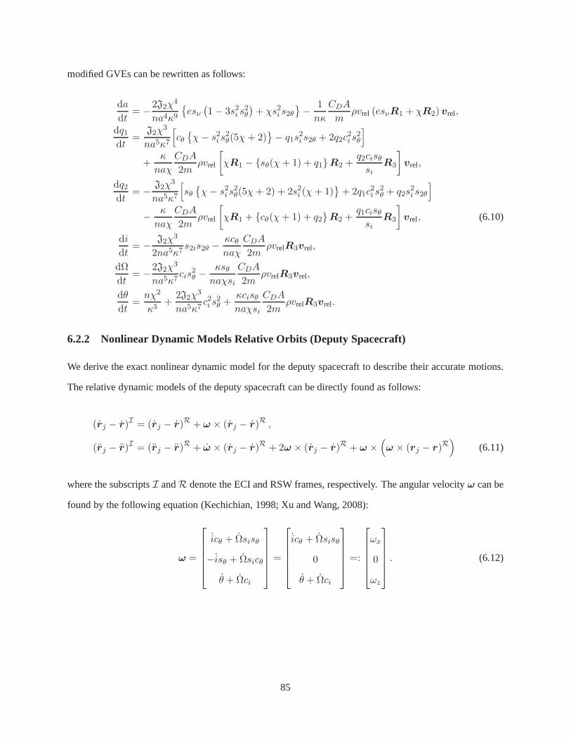
modified GVEs can be rewritten as follows:
da
dt= −2J2χ
4
na4κ9esν(1− 3s2i s
2θ
)+ χs2i s2θ
− 1
nκ
CDA
mρvrel (esνR1 + χR2)vrel,
dq1dt
=J2χ
3
na5κ7
[
cθχ− s2i s2θ(5χ+ 2)
− q1s2i s2θ + 2q2c
2i s
2θ
]
+κ
naχ
CDA
2mρvrel
[
χR1 − sθ(χ+ 1) + q1R2 +q2cisθsi
R3
]
vrel,
dq2dt
= − J2χ3
na5κ7
[
sθχ− s2i s2θ(5χ+ 2) + 2s2i (χ+ 1)
+ 2q1c
2i s
2θ + q2s
2i s2θ
]
− κ
naχ
CDA
2mρvrel
[
χR1 + cθ(χ+ 1) + q2R2 +q1cisθsi
R3
]
vrel, (6.10)
di
dt= − J2χ
3
2na5κ7s2is2θ −
κcθnaχ
CDA
2mρvrelR3vrel,
dΩ
dt= −2J2χ
3
na5κ7cis
2θ −
κsθnaχsi
CDA
2mρvrelR3vrel,
dθ
dt=nχ2
κ3+
2J2χ3
na5κ7c2i s
2θ +
κcisθnaχsi
CDA
2mρvrelR3vrel.
6.2.2 Nonlinear Dynamic Models Relative Orbits (Deputy Spacecraft)
We derive the exact nonlinear dynamic model for the deputy spacecraft to describe their accurate motions.
The relative dynamic models of the deputy spacecraft can be directly found as follows:
(rj − r)I = (rj − r)R +ω × (rj − r)R ,
(rj − r)I = (rj − r)R + ω × (rj − r)R + 2ω × (rj − r)R + ω ×(
ω × (rj − r)R)
(6.11)
where the subscriptsI andR denote the ECI and RSW frames, respectively. The angular velocity ω can be
found by the following equation (Kechichian, 1998; Xu and Wang, 2008):
ω =
icθ + Ωsisθ
−isθ + Ωsicθ
θ + Ωci
=
icθ + Ωsisθ
0
θ + Ωci
=:
ωx
0
ωz
. (6.12)
85
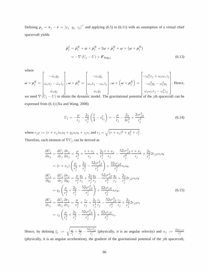
Definingρj = rj − r = [xj yj zj ]⊤ and applying (6.5) to (6.11) with an assumption of a virtual chief
spacecraft yields
ρIj = ρR
j + ω × ρRj + 2ω × ρR
j + ω ×(ω × ρR
j
)
= −∇ (Uj − U) + F drag,j (6.13)
where
ω × ρRj =
−ωzyj
ωzxj − ωxzj
ωxyj
, ω × ρRj =
−ωzyj
ωzxj − ωxzj
ωxyj
, ω×(
ω × ρRj
)
=
−ω2zxj + ωxωzzj
−ω2zyj − ω2
xyj
ωxωzxj − ω2xzj
. Hence,
we need∇ (Uj − U) to obtain the dynamic model. The gravitational potential ofthejth spacecraft can be
expressed from (6.1) (Xu and Wang, 2008)
Uj = −µ
rj− J2
r3j
(1
3− s2φj
)
= − µrj− J2
3r2j+
J2r2jZ
r5j(6.14)
whererjZ := (r + xj)sisθ + yjsicθ + zjci andrj =√
(r + xj)2 + y2j + z2j .
Therefore, each element of∇Uj can be derived as
∂Uj
∂xj=
dUj
drj
∂rj∂xj
=µ
r2j+r + xjrj
+J2
r4j
r + xjrj
−5J2r
2jZ
r6j
r + xjrj
+J2
r5j2rjZsisθ
= (r + xj)
(
µ
r3j+
J2
r5j−
5J2r2jZ
r7j
)
+2J2rjZr5j
sisθ,
∂Uj
∂yj=
dUj
drj
∂rj∂yj
=µ
r2j
yjrj
+J2
r4j
yjrj−
5J2r2jZ
r6j
yjrj
+J2
r5j2rjZsicθ
= yj
(
µ
r3j+
J2
r5j−
5J2r2jZ
r7j
)
+2J2rjZr5j
sicθ, (6.15)
∂Uj
∂zj=
dUj
drj
∂rj∂zj
=µ
r2j+zjrj
+J2
r4j
zjrj−
5J2r2jZ
r6j
zjrj
+J2
r5j2rjZci
= zj
(
µ
r3j+
J2
r5j−
5J2r2jZ
r7j
)
+2J2rjZr5j
ci.
Hence, by definingξj :=
√
µr3j
+ J2r5j− 5J2r2jZ
r7j(physically, it is an angular velocity) andαj :=
2J2rjZr5j
(physically, it is an angular acceleration), the gradient of the gravitational potential of thejth spacecraft,
86

∇Uj, becomes
∇Uj =
∂Uj
∂xj
∂Uj
∂yj
∂Uj
∂zj
=
ξ2j (r + xj) + αjsisθ
ξ2j yj + αjsicθ
ξ2j zj + αjci
. (6.16)
From (6.2) and (6.16),−∇ (Uj − U) can be obtained as follows:
−∇ (Uj − U) = −∇Uj +∇U =
−ξ2j (r + xj)− αjsisθ +µr2 + J2
r4 −3J2s2i s
2θ
r4
−ξ2j yj − αjsicθ +J2s2i s2θ
r4
−ξ2j zj − αjci +J2s2isθ
r4
. (6.17)
Therefore, from (6.13), (6.17), and (6.3), the relative dynamic models of thejth spacecraft with respect to
the formation center expressed in the RSW frame is expressedas
xj = ωzyj + 2ωz yj + ω2zxj − ωxωzzj − (r + xj)ξ
2j − αjsisθ
+ r
(µ
r3+
J2
r5− 3J2s
2i s
2θ
r5
)
− CDAj
2mjρjvj,relR1vj,rel + Fj,x
= 2ωz yj −(ξ2j − ω2
z
)xj + ωzyj − ωxωzzj − ξ2j r − αjsisθ
+
(µ
r3+
J2
r5− 5J2s
2i s
2θ
r5
)
r +2J2sisθr4
sisθ −CDAj
2mjρjvj,relR1vj,rel + Fj,x, (6.18)
yj = −ωzxj + ωxzj − 2ωzxj + 2ωxzj + ω2zyj + ω2
xyj − ξ2j yj − αjsicθ
+2J2sisθr4
sicθ −CDAj
2mjρjvj,relR2vj,rel + Fj,y,
zj = −ωxyj − 2ωxyj − ωxωzxj + ω2xzj − ξ2j zj − αjci
+2J2sisθr4
ci −CDAj
2mjρjvj,relR3vj,rel + Fj,z.
87

By definingξ :=√
µr3
+ J2r5− 5J2s2i s
2θ
r5andα := 2J2sisθ
r4, the exact nonlinear dynamic models for the deputy
spacecraft is obtained as
xj = 2ωz yj −(ξ2j − ω2
z
)xj + ωzyj − ωxωzzj −
(ξ2j − ξ2
)r
− (αj − α) sisθ −CDAj
2mjρjvj,relR1vj,rel + Fj,x,
yj = −2ωzxj + 2ωxzj − ωzxj −(ξ2j − ω2
x − ω2z
)yj + ωxzj (6.19)
− (αj − α) sicθ −CDAj
2mjρjvj,relR2vj,rel + Fj,y,
zj = −2ωxyj − ωxωzxj − ωxyj −(ξ2j − ω2
x
)zj
− (αj − α) ci −CDAj
2mjρjvj,relR3vj,rel + Fj,z.
Notice that (6.19) must be discretized to be used in the CD-SDRE controller.
6.2.3 The Discretization of Dynamic Models of the Relative Motion
For the discretization of the relative dynamic models, the sampling time is set toT . Then, (6.20) and (6.21)
show the discretization of the kinematics and dynamics of the relative motion:1
xj(k + 1) = xj + T xj, yj(k + 1) = yj + T yj, and zj(k + 1) = zj + T zj (6.20)
and the discretization of the dynamics of the relative motion (6.19):
xj(k + 1) = xj + 2Tωzyj − T(ξ2j − ω2
z
)xj + T ωzyj − Tωxωzzj − T
(ξ2j − ξ2
)r
− T (αj − α) sisθ − TCDAj
2mjρjvj,relR1vj,rel + TFj,x,
yj(k + 1) = −2Tωzxj + yj + 2Tωxzj − T ωzxj − T(ξ2j − ω2
x − ω2z
)yj + T ωxzj (6.21)
− T (αj − α) sicθ − TCDAj
2mjρjvj,relR2vj,rel + TFj,y,
zj(k + 1) = −2Tωxyj + zj − Tωxωzxj − T ωxyj − T(ξ2j − ω2
x
)zj
− T (αj − α) ci − TCDAj
2mjρjvj,relR3vj,rel + TFj,z.
1It should be noted that the time variablek at the right-hand side was removed for brevity.
88

By combining (6.20) and (6.21), the state-space equations of the relative motion are obtained:
xj
yj
zj
xj
yj
zj
+
︸ ︷︷ ︸
=:x+j
=
1 0 0 T 0 0
0 1 0 0 T 0
0 0 1 0 0 T
−T (ξ2j − ω2z) T ωz −Tωxωz 1 2Tωz 0
−T ωz −T (ξ2j − ω2x − ω2
z) T ωx −2Tωz 1 2Tωx
−Tωxωz −T ωx −T (ξ2j − ω2x) 0 −2Tωx 1
︸ ︷︷ ︸
=:Aj(xj)
xj
yj
zj
xj
yj
zj
︸ ︷︷ ︸
=:xj
+
0 0 0
0 0 0
0 0 0
T 0 0
0 T 0
0 0 T
︸ ︷︷ ︸
=:Bj
Fj,x
Fj,y
Fj,z
︸ ︷︷ ︸
uj
+
0
0
0
−T (ξ2j − ξ2)r − T (αj − α)sisθ − T CDAj
2mjρjvj,relR1vj,rel
−T (αj − α)sicθ − T CDAj
2mjρjvj,relR2vj,rel
−T (αj − α)ci − T CDAj
2mjρjvj,relR3vj,rel
︸ ︷︷ ︸
=:∆j
or in a simple form as
x+j = Aj(xj)xj +Bjuj +∆j . (6.22)
6.2.4 Extension to a Multiple Spacecraft System
In this part, we design the whole system of a multiple spacecraft system through the use of (6.22). For
notational simplicity, we will omit the timek in the following equations unless otherwise needed for clar-
ification. It is supposed thatjth spacecraft can communicate with other spacecraft in the formation. The
controller for thejth spacecraft can be designed as follows:
uj = −Kxj(xj)xj +Kωj
(xj)ωj +∑
l∈Nj ,l 6=j
(
KxlRl,jxl −Kωl
Rl,jωl
)
(6.23)
whereNj ⊂ Z1:N includes the indices for the spacecraft communicating withthejth spacecraft in the for-
mation. The matrix for a phase angle shiftRl,j is used to rotate the coordinates by a phase angle difference
89
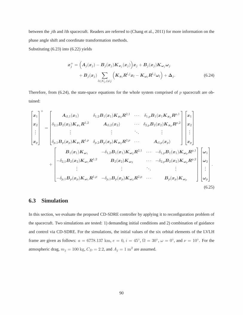
between thejth andlth spacecraft. Readers are referred to (Chang et al., 2011) for more information on the
phase angle shift and coordinate transformation methods.
Substituting (6.23) into (6.22) yields
x+j =
(
Aj(xj)−Bj(xj)Kxj(xj)
)
xj +Bj(xj)Kωjωj
+Bj(xj)∑
l∈Nj ,l 6=j
(
KxlRl,jxl −Kωl
Rl,jωl
)
+∆j. (6.24)
Therefore, from (6.24), the state-space equations for the whole system comprised ofp spacecraft are ob-
tained:
x1
x2
...
xp
+
=
Acl,1(x1) δ1,2B1(x1)Kx2R2,1 · · · δ1,pB1(x1KxpR
p,1
δ2,1B2(x2)Kx1R1,2 Acl,2(x2) · · · δ2,pB2(x2)KxpR
p,2
......
. . ....
δp,1Bp(xp)Kx1R1,p δp,2Bp(xp)Kx2R
2,p · · · Acl,p(xp)
x1
x2
...
xp
+
B1(x1)Kω1 −δ1,2B1(x1)Kω2R2,1 · · · −δ1,pB1(x1)KωpR
p,1
−δ2,1B2(x2)Kω1R1,2 B2(x2)Kω2 · · · −δ2,pB2(x2)KωpR
p,2
......
. . ....
−δp,1Bp(xp)Kω1R1,p −δp,1Bp(xp)Kω2R
2,p · · · Bp(xp)Kωp
ω1
ω2
...
ωp
.
(6.25)
6.3 Simulation
In this section, we evaluate the proposed CD-SDRE controller by applying it to reconfiguration problem of
the spacecraft. Two simulations are tested: 1) demanding initial conditions and 2) combination of guidance
and control via CD-SDRE. For the simulations, the initial values of the six orbital elements of the LVLH
frame are given as follows:a = 6778.137 km, e = 0, i = 45, Ω = 30, ω = 0, andν = 10. For the
atmospheric drag,mj = 100 kg, CD = 2.2, andAj = 1 m2 are assumed.
90
6.3.1 Controller Test with Extreme Initial Conditions
The purpose of the test is to show the reliability of the proposed CD-SDRE even with extremely demanding
initial condition. To this end, the desired trajectory of the spacecraft is generated by using the Hill-Clohessy-
Whiltshire (HCW) equation (Clohessy and Wiltshire, 1960) with the periodic conditions (Chang et al.,
2010a): y0 = −2nx0 andy0 = 2x0/n. We define such an orbit as a periodic relative orbit (PRO). The
initial conditions of the desired trajectory arex0 = y0 = 1 km, z0 = 0.5 km, z0 = 10−3 km/s. We want to
show how the spacecraft, initially at rest in the origin of the LVLH frame, follows its desired trajectory in
the presence of different levels of actuator saturations. The performance of the CD-SDRE is compared with
that by the linear MPC. For a consistent comparison, the sameweights of the controllers are chosen:Qk =
Q = diag([10−5, 10−5, 10−5, 10−6, 10−6, 10−6]
)andRk = R = diag
([1, 1, 1]
). For the CD-SDRE
and the Linear MPC,N = 30 andT = 1 sec. Three different input constraints are considered:0.5 m/s2,
0.3 m/s2, and0.1 m/s2, i.e.,−5× 10⁻⁴ ≤ Fx, Fy , Fz ≤ 5× 10⁻⁴,−3× 10⁻⁴ ≤ Fx, Fy, Fz ≤ 3× 10⁻⁴,
and−10−4 ≤ Fx, Fy , Fz ≤ 10−4, j = 1, 2, 3 for all k.
Figure 6.1 shows control profiles, state errors, and trajectories of the spacecraft with weak saturations:
−0.5 m/s2 ≤ Fx, Fy, Fz ≤ 0.5 m/s2. Although the constraints are relatively lenient, the propose CD-
SDRE effectively converge to the desire trajectory with less fuel consumption than that by the linear MPC.
As the constrains on the actuators become stringent (Figures 6.2 and 6.3), the spacecraft spent longer time
tracking and converging to its desired trajectory. The reason of having fluctuated trajectories before con-
verging to its desired trajectory is because of short lengthof the control horizonN = 30. In other words,
the proposed CD-SDRE and the linear MPC can look ahead only 30steps (i.e., 30 sec because the sampling
time is 1 sec.). The short control horizon can increase difficulties for the controllers to generate optimal con-
trol signals. However, even with such difficulties, the proposed CD-SDRE controller makes the spacecraft
converge to its desired trajectory faster (Table 6.1) with less fuel consumptions (∆V , Table 6.2).
We have shown the reliability of the proposed CD-SDRE controller. In general, however, spacecraft does
not have such fluctuated orbits while transferring its orbitalthough our main purpose of the test is to show
the reliability of the proposed CD-SDRE. In the next section, we evaluate guidance and control of spacecraft
with the proposed CD-SDRE to see the applicability of the proposed CD-SDRE in a realistic space mission.
91

Table 6.1: Comparison of Convergent Time [s] (Error< 0.1 m, i = x, y, z)
Constraints |Fi| ≤ 0.5m/s2 |Fi| ≤ 0.3m/s2 |Fi| ≤ 0.1m/s2
LMPC 175 230 636CD-SDRE 106 184 461
Table 6.2: Comparison of Total Fuel Consumption (∆V [km/s])
Constraints |Fi| ≤ 0.5m/s2 |Fi| ≤ 0.3m/s2 |Fi| ≤ 0.1m/s2
LMPC 0.09431 0.09306 0.09336CD-SDRE 0.06755 0.06828 0.06839
92
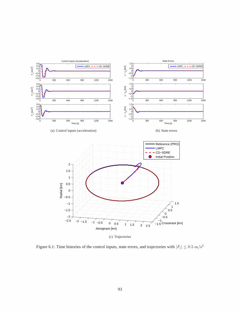
0 300 600 900 1200 1500−0.6−0.4−0.2
00.20.40.6
Control Inputs (Acceleration)
Fx [m
/s2 ]
LMPC CD−SDRE
0 300 600 900 1200 1500−0.6−0.4−0.2
00.20.40.6
Fy [m
/s2 ]
0 300 600 900 1200 1500−0.6−0.4−0.2
00.20.40.6
Fz [m
/s2 ]
Time [s]
(a) Control inputs (acceleration)
0 300 600 900 1200 1500−1.5
−1−0.5
00.5
11.5
State Errors
x −
xd [k
m]
LMPC CD−SDRE
0 300 600 900 1200 1500−1.5
−1−0.5
00.5
11.5
y −
yd [k
m]
0 300 600 900 1200 1500−1.5
−1−0.5
00.5
11.5
z −
zd [k
m]
Time [s]
(b) State errors
−2.5 −2 −1.5 −1 −0.5 0 0.5 1 1.5 2 2.5−1.5
−1−0.5
00.5
11.5
−2
−1.5
−1
−0.5
0
0.5
1
1.5
2
Crosstrack [km]
Alongtrack [km]
Rad
ial [
km]
Reference (PRO)LMPCCD−SDREInitial Position
(c) Trajectories
Figure 6.1: Time histories of the control inputs, state errors, and trajectories with|Fi| ≤ 0.5 m/s2
93
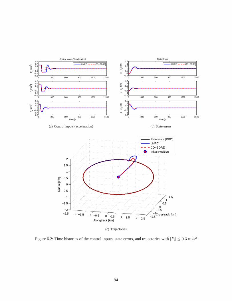
0 300 600 900 1200 1500−0.6−0.4−0.2
00.20.40.6
Control Inputs (Acceleration)
Fx [m
/s2 ]
LMPC CD−SDRE
0 300 600 900 1200 1500−0.6−0.4−0.2
00.20.40.6
Fy [m
/s2 ]
0 300 600 900 1200 1500−0.6−0.4−0.2
00.20.40.6
Fz [m
/s2 ]
Time [s]
(a) Control inputs (acceleration)
0 300 600 900 1200 1500−1.5
−1−0.5
00.5
11.5
State Errors
x −
xd [k
m]
LMPC CD−SDRE
0 300 600 900 1200 1500−1.5
−1−0.5
00.5
11.5
y −
yd [k
m]
0 300 600 900 1200 1500−1.5
−1−0.5
00.5
11.5
z −
zd [k
m]
Time [s]
(b) State errors
−2.5 −2 −1.5 −1 −0.5 0 0.5 1 1.5 2 2.5−1.5
−1−0.5
00.5
11.5
−2
−1.5
−1
−0.5
0
0.5
1
1.5
2
Crosstrack [km]
Alongtrack [km]
Rad
ial [
km]
Reference (PRO)LMPCCD−SDREInitial Position
(c) Trajectories
Figure 6.2: Time histories of the control inputs, state errors, and trajectories with|Fi| ≤ 0.3 m/s2
94
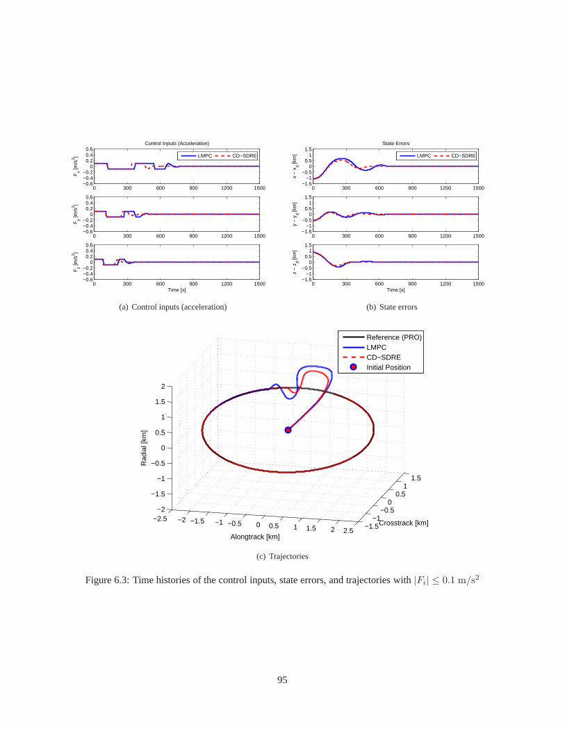
0 300 600 900 1200 1500−0.6−0.4−0.2
00.20.40.6
Control Inputs (Acceleration)
Fx [m
/s2 ]
LMPC CD−SDRE
0 300 600 900 1200 1500−0.6−0.4−0.2
00.20.40.6
Fy [m
/s2 ]
0 300 600 900 1200 1500−0.6−0.4−0.2
00.20.40.6
Fz [m
/s2 ]
Time [s]
(a) Control inputs (acceleration)
0 300 600 900 1200 1500−1.5
−1−0.5
00.5
11.5
State Errors
x −
xd [k
m]
LMPC CD−SDRE
0 300 600 900 1200 1500−1.5
−1−0.5
00.5
11.5
y −
yd [k
m]
0 300 600 900 1200 1500−1.5
−1−0.5
00.5
11.5
z −
zd [k
m]
Time [s]
(b) State errors
−2.5 −2 −1.5 −1 −0.5 0 0.5 1 1.5 2 2.5−1.5
−1−0.5
00.5
11.5
−2
−1.5
−1
−0.5
0
0.5
1
1.5
2
Crosstrack [km]
Alongtrack [km]
Rad
ial [
km]
Reference (PRO)LMPCCD−SDREInitial Position
(c) Trajectories
Figure 6.3: Time histories of the control inputs, state errors, and trajectories with|Fi| ≤ 0.1 m/s2
95
6.3.2 Extension to a Multiple Spacecraft System
In this section, we evaluate the proposed distributed CD-SDRE controller. From the formation flying sys-
tem obtained in the previous section, three different controllers are applied: a distributed CD-SDRE, a
linear MPC, and an infinite horizon LQR controller. For the simulation, the initial values of the six orbital
elements are given as follows:a = 6778.137 km, e = 0, i = 45, Ω = 30, ω = 0, andν = 10.
For the atmospheric drag,mj = 100 kg, CD = 2.2, andAj = 1 m2 are assumed. The desired trajec-
tories of the spacecraft are generated by using the Hill-Clohessy-Whiltshire (HCW) equation (Clohessy
and Wiltshire, 1960) with the periodic conditions (Chang etal., 2010a):y0 = −2nx0 andy0 = 2x0/n.
We define such an orbit as a periodic relative orbit (PRO). Theinitial conditions of the desired trajectories
arex0 = y0 = 1 km, z0 = 0.5 km, z0 = 10−3 km. The desired trajectories of the three spacecraft
are generated by using120 as the phase shift angle (Chang et al., 2011). Three spacecraft have random
initial positions and zero initial velocities. We want to show how the spacecraft, initially at rest, follow
their desired trajectories. For a consistent comparison, the same weights of the controllers are chosen:
Qk = Q = diag([10−5, 10−5, 10−5, 10−6, 10−6, 10−6]
)andRk = R = diag
([1, 1, 1]
). For the
distributed CD-SDRE and the Linear MPC,N = 30 andT = 1 sec. Three different input constraints
are considered:0.5 m/s2, 0.3 m/s2, and 0.1 m/s2, i.e., −5 × 10⁻⁴ ≤ Fx,j, Fy,j , Fz,j ≤ 5 × 10⁻⁴,
−3× 10⁻⁴ ≤ Fx,j, Fy,j , Fz,j ≤ 3× 10⁻⁴, and−10−4 ≤ Fx,j , Fy,j , Fz,j ≤ 10−4, j = 1, 2, 3 for all k.
The trajectories, state errors, and control inputs with different constraints on the control inputs. The red
circles show the initial positions of the spacecraft.
Figures 6.4 – 6.6 show simulation results of the trajectories, state errors, and control inputs of spacecraft
with different constraints on the control inputs. Notice that figures in Figures 6.4 – 6.6 show the state
errors and control inputs of the radial direction of the firstspacecraft for clarity since the results of the other
directions for three spacecraft are similar. From these results, the spacecraft with the proposed distributed
CD-SDRE controller are seen to converge to their trajectories faster and with smaller control effort than
those with the infinite LQR and the linear MPC. The LQR controller and the linear MPC have similar
results when the constraints are0.5 m/s2 and0.3 m/s2. However, the LQR controller makes the controlled
system unstable as the constraint become stringent. Moreover, we can also find the bigger wave motions in
the state trajectories as the constraints tighten. In the distributed CD-SDRE case, the wave motions could be
attenuated as the length of horizon increases, although also increasing the computational time. Therefore,
96
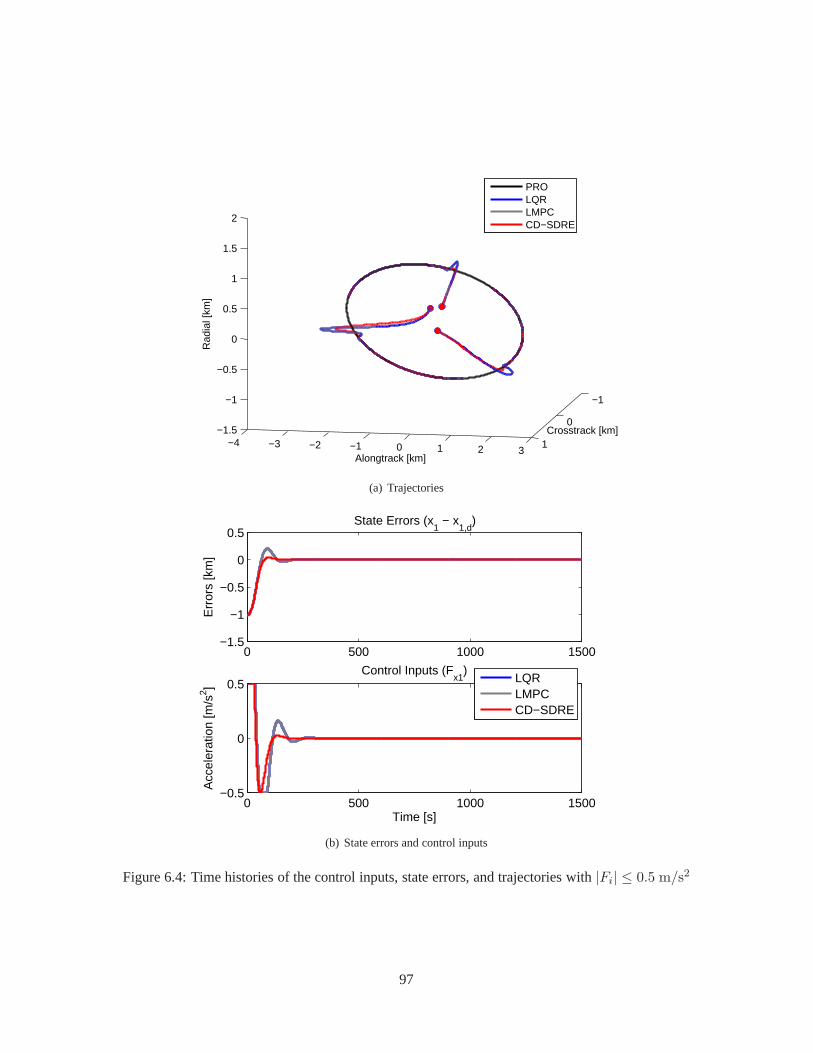
−4 −3 −2 −1 0 1 2 3
−1
0
1−1.5
−1
−0.5
0
0.5
1
1.5
2
Crosstrack [km]
Alongtrack [km]
Rad
ial [
km]
PROLQRLMPCCD−SDRE
(a) Trajectories
0 500 1000 1500−1.5
−1
−0.5
0
0.5State Errors (x
1 − x
1,d)
Err
ors
[km
]
0 500 1000 1500−0.5
0
0.5Control Inputs (F
x1)
Time [s]
Acc
eler
atio
n [m
/s2 ]
LQRLMPCCD−SDRE
(b) State errors and control inputs
Figure 6.4: Time histories of the control inputs, state errors, and trajectories with|Fi| ≤ 0.5 m/s2
97
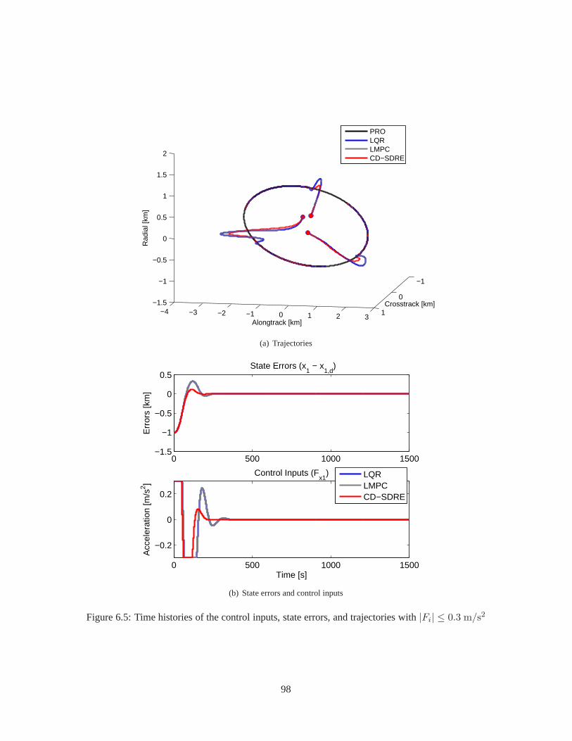
−4 −3 −2 −1 0 1 2 3
−1
0
1−1.5
−1
−0.5
0
0.5
1
1.5
2
Crosstrack [km]
Alongtrack [km]
Rad
ial [
km]
PROLQRLMPCCD−SDRE
(a) Trajectories
0 500 1000 1500−1.5
−1
−0.5
0
0.5State Errors (x
1 − x
1,d)
Err
ors
[km
]
0 500 1000 1500
−0.2
0
0.2
Control Inputs (Fx1
)
Time [s]
Acc
eler
atio
n [m
/s2 ]
LQRLMPCCD−SDRE
(b) State errors and control inputs
Figure 6.5: Time histories of the control inputs, state errors, and trajectories with|Fi| ≤ 0.3 m/s2
98

−4 −3 −2 −1 0 1 2 3
−1
0
1−1.5
−1
−0.5
0
0.5
1
1.5
2
Crosstrack [km]
Alongtrack [km]
Rad
ial [
km]
PROLQRLMPCCD−SDRE
(a) Trajectories
0 500 1000 1500−2
−1
0
1State Errors (x
1 − x
1,d)
Err
ors
[km
]
0 500 1000 1500−0.1
−0.05
0
0.05
0.1Control Inputs (F
x1)
Time [s]
Acc
eler
atio
n [m
/s2 ]
LQRLMPCCD−SDRE
(b) State errors and control inputs
Figure 6.6: Time histories of the control inputs, state errors, and trajectories with|Fi| ≤ 0.1 m/s2
99
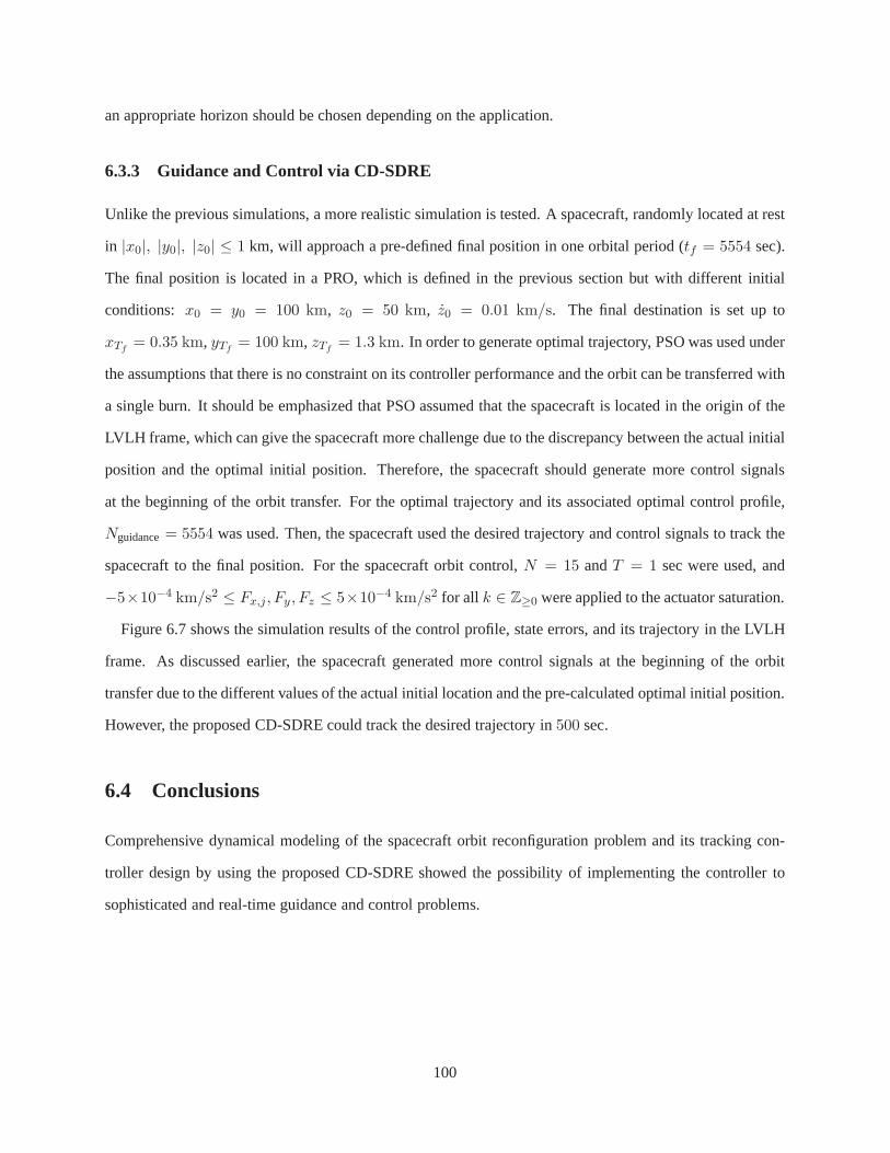
an appropriate horizon should be chosen depending on the application.
6.3.3 Guidance and Control via CD-SDRE
Unlike the previous simulations, a more realistic simulation is tested. A spacecraft, randomly located at rest
in |x0|, |y0|, |z0| ≤ 1 km, will approach a pre-defined final position in one orbital period (tf = 5554 sec).
The final position is located in a PRO, which is defined in the previous section but with different initial
conditions: x0 = y0 = 100 km, z0 = 50 km, z0 = 0.01 km/s. The final destination is set up to
xTf= 0.35 km, yTf
= 100 km, zTf= 1.3 km. In order to generate optimal trajectory, PSO was used under
the assumptions that there is no constraint on its controller performance and the orbit can be transferred with
a single burn. It should be emphasized that PSO assumed that the spacecraft is located in the origin of the
LVLH frame, which can give the spacecraft more challenge dueto the discrepancy between the actual initial
position and the optimal initial position. Therefore, the spacecraft should generate more control signals
at the beginning of the orbit transfer. For the optimal trajectory and its associated optimal control profile,
Nguidance= 5554 was used. Then, the spacecraft used the desired trajectory and control signals to track the
spacecraft to the final position. For the spacecraft orbit control, N = 15 andT = 1 sec were used, and
−5×10⁻⁴ km/s2 ≤ Fx,j, Fy , Fz ≤ 5×10⁻⁴ km/s2 for all k ∈ Z≥0 were applied to the actuator saturation.
Figure 6.7 shows the simulation results of the control profile, state errors, and its trajectory in the LVLH
frame. As discussed earlier, the spacecraft generated morecontrol signals at the beginning of the orbit
transfer due to the different values of the actual initial location and the pre-calculated optimal initial position.
However, the proposed CD-SDRE could track the desired trajectory in500 sec.
6.4 Conclusions
Comprehensive dynamical modeling of the spacecraft orbit reconfiguration problem and its tracking con-
troller design by using the proposed CD-SDRE showed the possibility of implementing the controller to
sophisticated and real-time guidance and control problems.
100
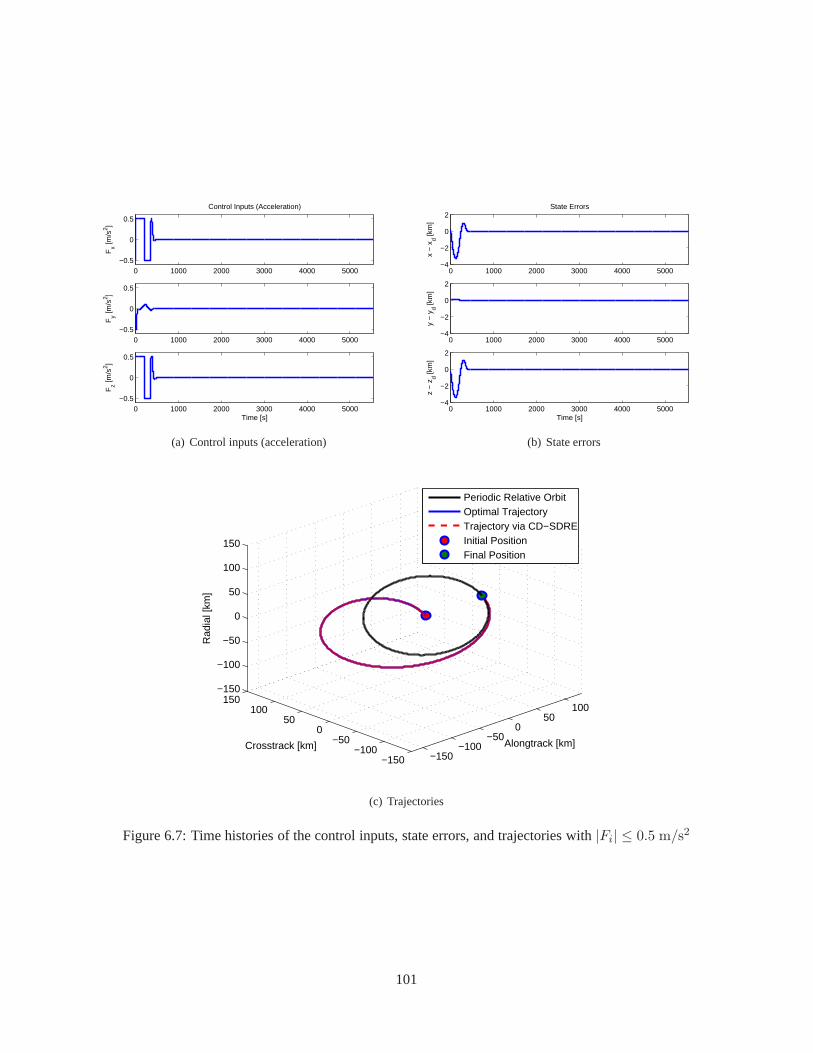
0 1000 2000 3000 4000 5000−0.5
0
0.5
Control Inputs (Acceleration)
Fx [m
/s2 ]
0 1000 2000 3000 4000 5000−0.5
0
0.5
Fy [m
/s2 ]
0 1000 2000 3000 4000 5000−0.5
0
0.5
Time [s]
Fz [m
/s2 ]
(a) Control inputs (acceleration)
0 1000 2000 3000 4000 5000−4
−2
0
2State Errors
x −
xd [k
m]
0 1000 2000 3000 4000 5000−4
−2
0
2
y −
yd [k
m]
0 1000 2000 3000 4000 5000−4
−2
0
2
Time [s]
z −
zd [k
m]
(b) State errors
−150−100
−500
50100
−150−100
−500
50100
150−150
−100
−50
0
50
100
150
Alongtrack [km]Crosstrack [km]
Rad
ial [
km]
Periodic Relative OrbitOptimal TrajectoryTrajectory via CD−SDREInitial PositionFinal Position
(c) Trajectories
Figure 6.7: Time histories of the control inputs, state errors, and trajectories with|Fi| ≤ 0.5 m/s2
101

Chapter 7
Robust Constrained Discrete-TimeState-Dependent Riccati EquationController
7.1 Introduction
THE constrained discrete-time state-dependent Riccati equation (CD-SDRE) technique in the presence
of uncertainties in the nonlinear system to be controlled ispresented. The proposed robust CD-SDRE
controller is given by a switched control law that incorporates D-SDRE and MPC-based controllers. First,
the system stability under each of the latter controllers isseparately established. The stability of the closed
loop system under a robust CD-SDRE controller is then provenbased on the stability of each control system
comprising switching configuration. A high fidelity dynamical model of spacecraft attitude motion in 3-
dimensional space is derived with a partially filled fuel tank, assumed to have the first fuel slosh mode. The
proposed robust CD-SDRE controller is then applied to the spacecraft attitude control system to stabilize its
motion in the presence of uncertainly characterized by the first fuel slosh mode. The resulting performance
demonstrates the reliability of the proposed robust CD-SDRE technique.
This chapter is organized as follows. In the following section, the robust D-SDRE feedback controller in
the presence of uncertainties is investigated. Stability conditions of robust MPC mode and finally the robust
CD-SDRE in the presence of uncertainties are provided in Section 7.4. In Section 7.5, nonlinear dynamics
of spacecraft attitude dynamics is derived and simulated with the proposed CD-SDRE controller. Finally,
concluding remarks are made in Section 7.6.
7.2 Review of D-SDRE Technique
The D-SDRE technique was investigated in Chapter 5. However, we briefly review it here for notational
clarification.
102
7.2.1 Derivation of the D-SDRE Feedback Controller
Consider the discrete-time deterministic nonlinear control-affine system described by the nonlinear differ-
ence equation:
zk+1 = f(zk, uk) = A(zk)zk +B(zk)uk (7.1)
wherezk ∈ X ⊆ Rn and uk ∈ U ⊆ R
m. It is assumed thatf(0) = 0 and f(zk) is continuously
differentiable. We assume that(A(zk),B(zk)) is piecewise controllable for allzk ∈ X. For this system,
the D-SDRE technique finds a control inputuk ∈ U at each time that minimizes the following performance
index:
J0 =1
2
k+N−1∑
j=k
(
z⊤j Q(zj)zj + u⊤
j R(zj)uj
)
(7.2)
where the weightsQ(zj) andR(zj) are assumed to be symmetric positive semi-definite and symmetric
positive definite, respectively.
The optimal feedback controluk for the deterministic system (7.1) is defined as follows:
u(zk) = −(
R(zk) +B(zk)⊤P k+1B(zk)
)−1B(zk)
⊤P k+1A(zk)zk =: −K(zk)zk (7.3)
whereK(zk) ∈ Rm×n is the optimal feedback control gain of the D-SDRE technique.
It should be noted thatP k andP k+1 are needed to obtainK(zk) whereP k andP k+1 are the solutions of
the generalized discrete-time Riccati equation (GD-RE) attimesk andk + 1, respectively:
P k =
(
Q(zk) +1
2z⊤k
∂Q(zk)
∂zk− 1
2u⊤k
∂R(zk)
∂zkK(zk)
)
+ A⊤P k+1
(
I +B(zk)R(zk)−1B(zk)
⊤P k+1
)−1A(zk). (7.4)
7.3 D-SDRE for Uncertain Nonlinear Systems
Consider the discrete-time nonlinear system with uncertainties:
xk+1 = f(xk,uk,∆k) = (A(xk) +∆Ak)xk + (B(xk) +∆Bk
)uk (7.5)
103
wherexk ∈ X ⊆ Rn anduk ∈ U ⊆ R
m. The parameters∆Akand∆Bk
are, respectively, uncertainties of
A(xk) andB(xk) with the following assumptions
‖∆Ak‖ ≤ a and ‖∆Bk
‖ ≤ b (7.6)
for all xk ∈ X.
By means of the D-SDRE controller for the deterministic nonlinear system (7.1), we want to find a
control inputuk such that the uncertain nonlinear system (7.5) is stabilized. It should be noted that the
deterministic nonlinear system (7.1) will be considered tobe a nominal system of (7.5) throughout this
chapter. The following lemma will play an important role in proving the stability of the D-SDRE feedback
controller of (7.5) in the presence of uncertainties.
Lemma 18 Consider a linear discrete-time system
xk+1 = A(α)xk +B(β)uk (7.7)
whereA(α) ∈ A := A(α) : A(α) =∑LA
i=1 αiAi,∑LA
i=1 αi = 1, αi ≥ 0 andB(β) ∈ B := B(β) :
B(β) =∑LB
i=1 βjBj,∑LB
j=1 βj = 1, βj ≥ 0. Then (7.7) is robustly stable inA and B if there exist
P ij = P⊤ij > 0 andG such that
P ij AiG−BjK
G⊤A⊤i − K
⊤B⊤
j G+G⊤ − P ij
> 0 (7.8)
for all i ∈ Z1:LAandj ∈ Z1:LB
. Then a robust state feedback controller is obtained by
uk = −Kxk = −KG−1xk. (7.9)
Proof See de Oliveira et al. (1999).
For the stability proof, the uncertain nonlinear system (7.5) can be rewritten in the following form:
xk+1 = Axk(α)xk +Bxk
(β)uk (7.10)
104
whereAxk(α) ∈ Axk
:= Axk(α) : Axk
(α) =∑LA
i=1 αiAxk,i;∑LA
i=1 = 1, αi ≥ 0 andBxk(β) ∈
Bxk:= Bxk
(β) : Bxk(β) =
∑LB
j=1 βjBxk,j;∑LB
j=1 = 1, βj ≥ 0 whereAxk,i andBxk,j are the vertices
of the polytopesAxkandBxk
, respectively.
With the uncertain nonlinear system, we can design a robust state feedback controller via the discrete-time
state-dependent Riccati equation.
Theorem 19 Given the nonlinear system (7.10) and the nominal state feedback control inputuk = −K(zk)zk,
there exists a matrixGk satisfying
P ij Axk,iGk −Bxk,jK(zk)
G⊤k A
⊤xk,i− K
⊤(zk)B
⊤xk,j
Gk +G⊤k −P ij
> 0 (7.11)
for all i ∈ Z1:LA, j ∈ Z1:LB
∀xk ∈ X ∈ Rn such that the state feedback controlleruk = −K(xk)xk =
−K(zk)G−1k xk robustly stabilizes the uncertain nonlinear system.
Proof The proof is straightforward from Lemma 18 by using piecewisexk for all k ∈ Z≥0.
7.4 CD-SDRE for Uncertain Nonlinear Systems
As one of the control modes in CD-SDRE, the robust MPC is analyzed in this section. Then, we investigate
the CD-SDRE technique to control uncertain nonlinear systems.
7.4.1 Robust Stability Analysis of MPC Mode
The robust MPC controller contains two controllers: a nominal MPC-based controller and a supplemental
controller to handle uncertainties in the nominal systems,which is the same as the uncertain nonlinear
system (Rawlings and Mayne, 2009). First, we consider the nominal controller. Given a discrete-time
nonlinear control-affine system (7.1), we want to find a sequence of optimal control signals:
µN (zk, k) := µk(zk, k), µk+1(zk, k), · · · , µk+N−1(zk, k) (7.12)
105
that minimizes the following performance index
JN (zk) =
k+N−1∑
i=k
(
z⊤i Q(zi)zi + u⊤
i R(zi)ui
)
+ z⊤k+NS(zk+N )zk+N (7.13)
subject to (7.1),zk ∈ X, anduk ∈ U whereX is convex and closed inRn andU is convex and compact in
Rm both of which contain their origins.
By solving the constrained optimization problem, an optimal control sequenceµN (zk, k) can be obtained.
Then the the nominal MPC-based controller is designed asuk := µk(zk, k) whereµk(zk, k) is in (7.12).
The following assumptions are needed to prove the stabilityof the nominal system controlled by MPC.
Assumption 20 The stage cost and the terminal cost satisfy the bound conditions
∑k+N−1i=k z⊤
i Q(zi)zi + u⊤i R(zi)ui ≥ α1(|zk|)
z⊤k+NS(zk+N )zk+N ≤ α2(|zk|)
∀zk ∈ XN , ∀uk ∈ U and∀zk ∈ XN whereα1(·), α2(·) ∈ K∞ andXN ∈ X is the ROA of the system
controlled by MPC.
Assumption 21 The following inequality holds for allk ∈ Z≥0:
minu∈U
k+N−1∑
i=k
(
z⊤i Q(zi)zi+ u⊤
i R(zi)ui
)
+z⊤k+NS(zk+N )zk+N ≤ z⊤
k+N−1S(zk+N−1)zk+N−1. (7.14)
The following theorem can be proven with the assumptions.
Theorem 22 Given the discrete-time deterministic nonlinear control-affine system (7.1), the performance
index in (7.13), and the optimal control sequence (7.12), there existα1(·), α2(·) ∈ K∞ such thatJN (·)
satisfies the following inequalities:
JN (zk) ≥ α1(|zk|) ∀zk ∈ XN
JN (zk) ≤ α2(|zk|) ∀zk ∈ XN
JN (zk+1)− JN (zk) ≤ −α1(|zk|) ∀zk ∈ XN .
(7.15)
Proof See Proposition 2.18 in Rawlings and Mayne (2009).
106

Theorem 22 shows that the system controlled by MPC is exponentially stable inXN .
In order to design the second part of the MPC-based controller which is responsible for reducing the error
between actual statesxk and the nominal stateszk, we consider the following composite system:
xk+1 = A(xk)xk +B(xk)uk
zk+1 = A(zk)zk +B(zk)uk.(7.16)
We want to design a sequence of optimal control signals:
µN (xk,zk, k) :=µk(xk,zk, k), µk+1(xk,zk, k), · · · , µk+N−1(xk,zk, k)
(7.17)
that minimizes the following performance index
JN (xk,zk) =
k+N−1∑
i=k
(
(xi − zi)⊤Q(zi)(xi − zi) + (ui − ui)
⊤R(zi)(ui − ui))
(7.18)
subject to (7.16),xk,zk ∈ X, anduk, uk ∈ U whereX is convex and closed inRn andU is convex and
compact inRm both of which contain their origins.
Theorem 23 The composite system (7.16) together withuk = µk(xk,zk, k) and uk = µk(xk,zk, k) is
exponentially stable in the ROAXN ∈ X wherexk,zk ∈ XN ∀k ∈ Z≥0.
Proof To prove the robust stability of the MPC mode, it is assumed that the control signals can be
expressed as
uk = −KMPCxk −K ′MPCzk −KMPC,0
uk = −KMPCzk −K′MPCzk −KMPC,0.
(7.19)
Substituting (7.19) into (7.16) yields
xk+1 = Acl(xk)xk (7.20)
wherexk =
[
x⊤k z⊤
k 1
]⊤
.
The stability is proven straightforwardly from Theorem 7 byreplacingA(xk) by Acl(xk).
We have shown that the uncertain nonlinear discrete-time system controlled by D-SDRE and MPC is ex-
ponentially stable in its ROA. Since only one controller is activated during each sampling time, the proposed
107
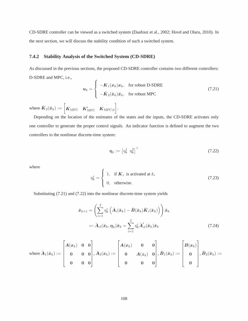
CD-SDRE controller can be viewed as a switched system (Daafouz et al., 2002; Hovd and Olaru, 2010). In
the next section, we will discuss the stability condition ofsuch a switched system.
7.4.2 Stability Analysis of the Switched System (CD-SDRE)
As discussed in the previous sections, the proposed CD-SDREcontroller contains two different controllers:
D-SDRE and MPC, i.e.,
uk =
−K1(xk)xk, for robust D-SDRE
−K2(xk)xk, for robust MPC(7.21)
whereK2(xk) :=
[
KMPC K ′MPC KMPC,0
]
.
Depending on the location of the estimates of the states and the inputs, the CD-SDRE activates only
one controller to generate the proper control signals. An indicator function is defined to augment the two
controllers to the nonlinear discrete-time system:
ηk :=[η1k η2k
]⊤(7.22)
where
ηik =
1, if Ki is activated atk,
0, otherwise.(7.23)
Substituting (7.21) and (7.22) into the nonlinear discrete-time system yields
xk+1 =
(2∑
i=1
ηik
(
Ai(xk)− B(xk)Ki(xk)))
xk
=: Acl(xk,ηk)xk =
2∑
i=1
ηikAicl(xk)xk (7.24)
whereA1(xk) :=
A(xk) 0 0
0 0 0
0 0 0
, A2(xk) :=
A(xk) 0 0
0 A(zk) 0
0 0 0
, B1(xk) :=
B(xk)
0
0
, B2(xk) :=
108
B(xk)
B(zk)
0
, andK1(xk) :=
[
K1(xk) 0 0
]
.
The following theorem shows the stability condition of the switched system.
Theorem 24 Suppose there exist symmetric positive definite matricesM1k (D-SDRE) andM2
k (MPC) such
that
M ik A
i⊤cl M
jk
MjkA
icl M
jk
> 0 ∀i, j ∈ Z0:1. (7.25)
Then, the switched system (7.24) is exponentially stable inXN .
Proof Since the stability condition of the nonlinear discrete-time system controlled by D-SDRE and
MPC was proven, there existM1k andM2
k such that
M1k A
1⊤cl M
1k
M 1kA
1cl M1
k
> 0, and
M2k A
2⊤cl M
2k
M2kA
2cl M 2
k
> 0 ∀k ∈ Z≥0. (7.26)
Since we consider the two modes (D-SDRE and the MPC) together, we need to combine matrices in (7.26):
M ik
∑2l=1 η
lk A
i⊤cl M
jk
∑2l=1 η
lk
Mjk
∑2l=1 η
lkA
icl M
jk
∑2l=1 η
lk
> 0. (7.27)
It is sufficient to show that the inequality holds fori 6= j. Let η1k = 1 at timek andη2k = 1 at timek + 1
since the inequalities in (7.26) hold forη1k = 1 ∀k ∈ Z≥0 andη2k = 1 ∀k ∈ Z≥0, respectively. Then
M ik A
i⊤cl M
jk+1
Mjk+1A
icl M
jk+1
> 0. (7.28)
By Schur complement (Boyd et al., 1994), it is equivalent to the following inequality,
x⊤k
(
M ik − Ai⊤
cl Mjk+1A
icl
)
xk > 0. (7.29)
109
The Lyapunov function candidate for the switched system is defined as
V (xk) := x⊤k M k(ηk)xk = x⊤
k
(2∑
l=1
ηlkMlk
)
xk (7.30)
whereM ik is symmetric positive definite, defined in (7.26).
Hence, the following inequalities hold due to the definitionof theV (xk) andM ik:
V (xk) ≥ λmin(minM1k, M
2k)|xk| =: α1(|xk|)
V (xk) ≤ λmax(maxM1k, M
2k)|xk| =: α2(|xk|).
(7.31)
The following inequality can be derived by the definition of the Lyapunov function
V (xk+1)− V (xk) = x⊤k+1
(2∑
l=1
ηlk+1Mlk+1
)
xk+1 − x⊤k
(2∑
l=1
ηlkMlk
)
xk
= −x⊤k
(
M ik − A
i⊤cl M
jk+1A
icl,k
)
xk
≤ −α3(|xk|) < 0 (7.32)
whereα3 ∈ K∞.
This proves the theorem.
We have shown the concept, the mechanism, and the stability condition of the CD-SDRE controller in the
presence of uncertainties. We evaluate the proposed controller in the following section.
7.5 Numerical Evaluation
In order to evaluate the performance of the proposed CD-SDREcontroller in the presence of uncertainties
in the plant, a challenging problem is considered: spacecraft attitude control in the presence fuel slosh effect
and limited actuator performance. To this end, we first derive the equations of motion for the spacecraft
attitude.
110
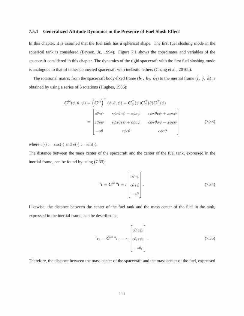
7.5.1 Generalized Attitude Dynamics in the Presence of FuelSlosh Effect
In this chapter, it is assumed that the fuel tank has a spherical shape. The first fuel sloshing mode in the
spherical tank is considered (Bryson, Jr., 1994). Figure 7.1 shows the coordinates and variables of the
spacecraft considered in this chapter. The dynamics of the rigid spacecraft with the first fuel sloshing mode
is analogous to that of tether-connected spacecraft with inelastic tethers (Chang et al., 2010b).
The rotational matrix from the spacecraft body-fixed frame (b1, b2, b3) to the inertial frame (i, j, k) is
obtained by using a series of 3 rotations (Hughes, 1986):
Cbi(φ, θ, ψ) =(
Cib)⊤
(φ, θ, ψ) = C⊤3 (ψ)C
⊤2 (θ)C
⊤1 (φ)
=
cθcψ sφsθcψ − cφsψ cφsθcψ + sφsψ
cθsψ sφsθsψ + cφcψ cφsθsψ − sφcψ
−sθ sφcθ cφcθ
(7.33)
wherec(·) := cos(·) ands(·) := sin(·).
The distance between the mass center of the spacecraft and the center of the fuel tank, expressed in the
inertial frame, can be found by using (7.33):
il = Cbi bl = l
cθcψ
cθsψ
−sθ
. (7.34)
Likewise, the distance between the center of the fuel tank and the mass center of the fuel in the tank,
expressed in the inertial frame, can be described as
irf = Csi srf = rf
cθfcψf
cθfsψf
−sθf
. (7.35)
Therefore, the distance between the mass center of the spacecraft and the mass center of the fuel, expressed
111
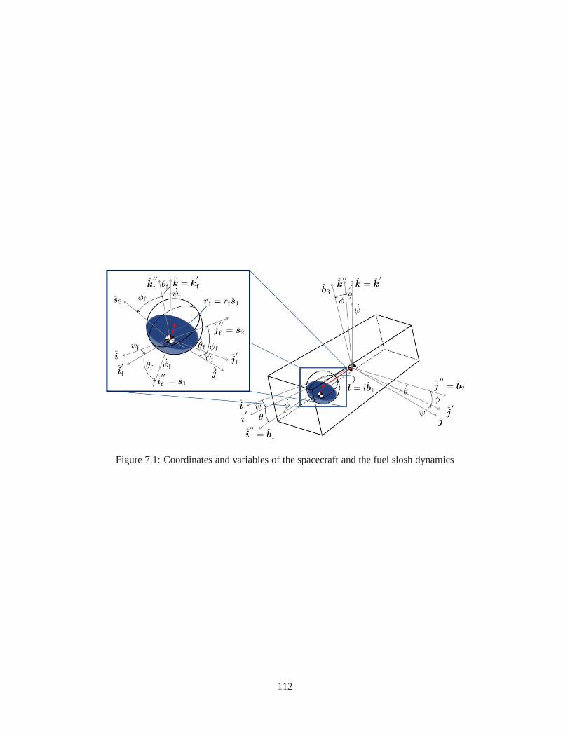
Figure 7.1: Coordinates and variables of the spacecraft andthe fuel slosh dynamics
112
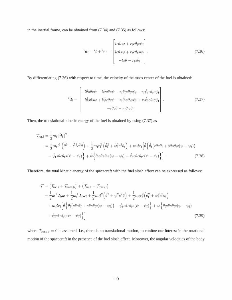
in the inertial frame, can be obtained from (7.34) and (7.35)as follows:
idf =il + irf =
lcθcψ + rfcθfcψf
lcθsψ + rfcθfsψf
−lsθ − rfsθf
. (7.36)
By differentiating (7.36) with respect to time, the velocity of the mass center of the fuel is obtained:
idf =
−lθsθcψ − lψcθsψ − rf θfsθfcψf − rfψfcθfsψf
−lθsθsψ + lψcθcψ − rf θfsθfsψf + rfψfcθfcψf
−lθcθ − rf θfcθf
. (7.37)
Then, the translational kinetic energy of the fuel is obtained by using (7.37) as
Trot,f =1
2mf‖df‖2
=1
2mfl
2(
θ2 + ψ2c2θ)
+1
2mfr
2f
(
θ2f + ψ2f c
2θf
)
+mflrf
[
θ
θf(cθcθf + sθsθfc(ψ − ψf)
)
− ψfsθcθfs(ψ − ψf)
+ ψ
θfcθsθfs(ψ − ψf) + ψfcθcθfc(ψ − ψf)]
. (7.38)
Therefore, the total kinetic energy of the spacecraft with the fuel slosh effect can be expressed as follows:
T =(Trot,b + Ttrans,b
)+(Trot,f + Ttrans,f
)
=1
2ω⊤Ibω +
1
2ω⊤
f I fωf +1
2mfl
2(
θ2 + ψ2c2θ)
+1
2mfr
2f
(
θ2f + ψ2f c
2θf
)
+mflrf
[
θ
θf(cθcθf + sθsθfc(ψ − ψf)
)− ψfsθcθfs(ψ − ψf)
+ ψ
θfcθsθfs(ψ − ψf)
+ ψfcθcθfc(ψ − ψf)]
(7.39)
whereTtrans,b = 0 is assumed, i.e., there is no translational motion, to confine our interest in the rotational
motion of the spacecraft in the presence of the fuel slosh effect. Moreover, the angular velocities of the body
113

and the fuel respect to the inertial frame, respectively, can be expressed as
ω :=
ω1
ω2
ω3
=
φ− ψsθ
θcφ+ ψcθsφ
−θsφ+ ψcθcφ
and ωf :=
ωf,1
ωf,2
ωf,3
=
φf − ψfsθf
θfcφf + ψfcθfsφf
−θfsφf + ψfcθfcφf
. (7.40)
By assuming that the potential energy of the spacecraft is negligible (i.e.,V ≈ 0), the Lagrangian of the
system is the same as the total kinetic energy in (7.39), i.e.,
L = T − V = T . (7.41)
In order to derive the equations of motion of the spacecraft in the presence of the fuel slosh effect, Lagrange’s
equations of motion is used (Goldstein et al., 2002):
d
dt
(∂L∂q
)
− ∂L∂q
+∂R∂q
= τ (7.42)
whereq := [φ θ ψ φf θf ψf ]⊤ is the generalized coordinates andR :=
∑εiq
2i is Rayleigh’s dissipation
function.
By the assumption of the first fuel slosh mode, we can obtain constraints in the rotational motion of the fuel
slosh:
θfcφf = −ψfcθfsφf
θfsφf = ψfcθfcφf.(7.43)
The nonlinear equations of motion of the spacecraft with thefirst fuel slosh mode are derived by solving
(7.42) together with the constraints (7.43). The equationsof motion of the spacecraft attitude in the presence
114
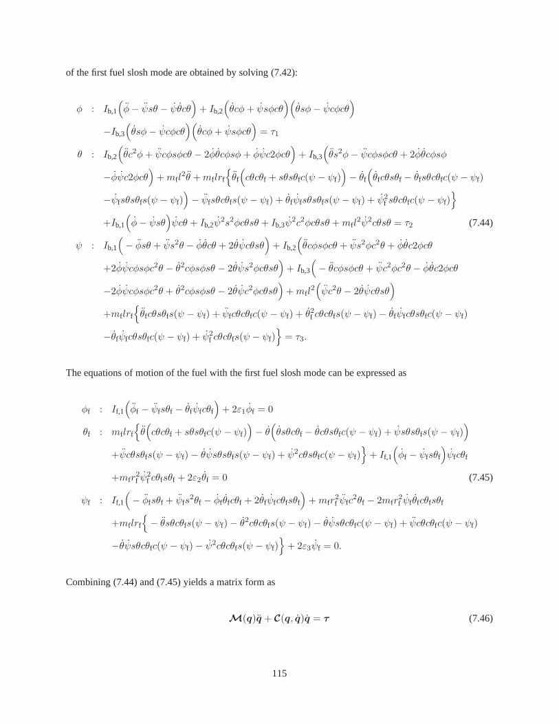
of the first fuel slosh mode are obtained by solving (7.42):
φ : Ib,1
(
φ− ψsθ − ψθcθ)
+ Ib,2
(
θcφ+ ψsφcθ)(
θsφ− ψcφcθ)
−Ib,3
(
θsφ− ψcφcθ)(
θcφ+ ψsφcθ)
= τ1
θ : Ib,2
(
θc2φ+ ψcφsφcθ − 2φθcφsφ+ φψc2φcθ)
+ Ib,3
(
θs2φ− ψcφsφcθ + 2φθcφsφ
−φψc2φcθ)
+mfl2θ +mf lrf
θf
(
cθcθf + sθsθfc(ψ − ψf))
− θf
(
θfcθsθf − θfsθcθfc(ψ − ψf)
−ψfsθsθfs(ψ − ψf))
− ψfsθcθfs(ψ − ψf) + θfψfsθsθfs(ψ − ψf) + ψ2f sθcθfc(ψ − ψf)
+Ib,1
(
φ− ψsθ)
ψcθ + Ib,2ψ2s2φcθsθ + Ib,3ψ
2c2φcθsθ +mfl2ψ2cθsθ = τ2 (7.44)
ψ : Ib,1
(
− φsθ + ψs2θ − φθcθ + 2θψcθsθ)
+ Ib,2
(
θcφsφcθ + ψs2φc2θ + φθc2φcθ
+2φψcφsφc2θ − θ2cφsφsθ − 2θψs2φcθsθ)
+ Ib,3
(
− θcφsφcθ + ψc2φc2θ − φθc2φcθ
−2φψcφsφc2θ + θ2cφsφsθ − 2θψc2φcθsθ)
+mfl2(
ψc2θ − 2θψcθsθ)
+mflrf
θfcθsθfs(ψ − ψf) + ψfcθcθfc(ψ − ψf) + θ2f cθcθfs(ψ − ψf)− θfψfcθsθfc(ψ − ψf)
−θfψfcθsθfc(ψ − ψf) + ψ2f cθcθfs(ψ − ψf)
= τ3.
The equations of motion of the fuel with the first fuel slosh mode can be expressed as
φf : If,1
(
φf − ψfsθf − θfψfcθf
)
+ 2ε1φf = 0
θf : mflrf
θ(
cθcθf + sθsθfc(ψ − ψf))
− θ(
θsθcθf − θcθsθfc(ψ − ψf) + ψsθsθfs(ψ − ψf))
+ψcθsθfs(ψ − ψf)− θψsθsθfs(ψ − ψf) + ψ2cθsθfc(ψ − ψf)
+ If,1
(
φf − ψfsθf
)
ψfcθf
+mfr2f ψ
2f cθfsθf + 2ε2θf = 0 (7.45)
ψf : If,1
(
− φfsθf + ψfs2θf − φf θfcθf + 2θfψfcθfsθf
)
+mfr2f ψfc
2θf − 2mfr2f ψf θfcθfsθf
+mflrf
− θsθcθfs(ψ − ψf)− θ2cθcθfs(ψ − ψf)− θψsθcθfc(ψ − ψf) + ψcθcθfc(ψ − ψf)
−θψsθcθfc(ψ − ψf)− ψ2cθcθfs(ψ − ψf)
+ 2ε3ψf = 0.
Combining (7.44) and (7.45) yields a matrix form as
M(q)q + C(q, q)q = τ (7.46)
115
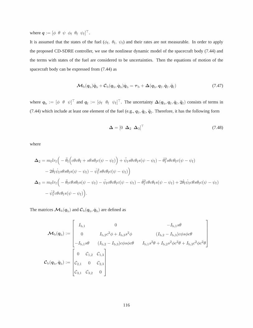
whereq := [φ θ ψ φf θf ψf ]⊤.
It is assumed that the states of the fuel (φf, θf, ψf) and their rates are not measurable. In order to apply
the proposed CD-SDRE controller, we use the nonlinear dynamic model of the spacecraft body (7.44) and
the terms with states of the fuel are considered to be uncertainties. Then the equations of motion of the
spacecraft body can be expressed from (7.44) as
Mb(qb)qb + Cb(qb, qb)qb = τ b +∆(qb, qf , qf , qf) (7.47)
whereqb := [φ θ ψ]⊤ andqf := [φf θf ψf ]⊤. The uncertainty∆(qb, qf , qf , qf) consists of terms in
(7.44) which include at least one element of the fuel (e.g.,qf , qf , qf . Therefore, it has the following form
∆ = [0 ∆2 ∆3]⊤ (7.48)
where
∆2 = mf lrf
(
− θf(
cθcθf + sθsθfc(ψ − ψf))
+ ψfsθcθfs(ψ − ψf)− θ2f sθcθfc(ψ − ψf)
− 2θf ψfsθsθfs(ψ − ψf)− ψ2f sθcθfc(ψ − ψf)
)
∆3 = mf lrf
(
− θfcθsθfs(ψ − ψf)− ψfcθcθfc(ψ − ψf)− θ2f cθcθfs(ψ − ψf) + 2θf ψfcθsθfc(ψ − ψf)
− ψ2f cθcθfs(ψ − ψf)
)
.
The matricesMb(qb) andCb(qb, qb) are defined as
Mb(qb) :=
Ib,1 0 −Ib,1sθ
0 Ib,2c2φ+ Ib,3s
2φ (Ib,2 − Ib,3)cφsφcθ
−Ib,1sθ (Ib,2 − Ib,3)cφsφcθ Ib,1s2θ + Ib,2s
2φc2θ + Ib,3c2φc2θ
Cb(qb, qb) :=
0 C1,2 C1,3C2,1 0 C2,3C3,1 C3,2 0
116
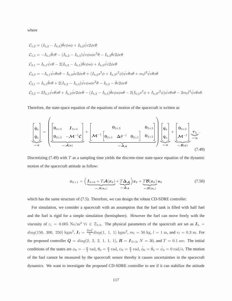
where
C1,2 = (Ib,2 − Ib,3)θcφsφ+ Ib,2ψc2φcθ
C1,3 = −Ib,1θcθ − (Ib,2 − Ib,3)ψcφsφc2θ − Ib,3θc2φcθ
C2,1 = Ib,1ψcθ − 2(Ib,2 − Ib,3)θcφsφ+ Ib,2ψc2φcθ
C2,3 = −Ib,1ψcθsθ − Ib,3φc2φcθ + (Ib,2s2φ+ Ib,3c
2φ)ψcθsθ +mf l2ψcθsθ
C3,1 = Ib,1θcθ + 2(Ib,2 − Ib,3)ψcφsφc2θ − Ib,3 − θc2φcθ
C3,2 = 2Ib,1ψcθsθ + Ib,2φc2φcθ − (Ib,2 − Ib,3)θcφsφsθ − 2(Ib,2s2φ+ Ib,3c
2φ)ψcθsθ − 2mf l2ψcθsθ.
Therefore, the state-space equation of the equations of motion of the spacecraft is written as
qb
qb
︸ ︷︷ ︸
=:x
=
03×3 I3×3
03×3 −M−1C
︸ ︷︷ ︸
=:A(x)
+
03×3 03×3
M−1
[
03×1 ∆θ−103×1
]
03×3
︸ ︷︷ ︸
=:∆A
qb
qb
︸ ︷︷ ︸
=:x
+
03×3
M−1
︸ ︷︷ ︸
=:B(x)
τ b︸︷︷︸
=:u
.
(7.49)
Discretizing (7.49) withT as a sampling time yields the discrete-time state-space equation of the dynamic
motion of the spacecraft attitude as follow:
xk+1 =(
I6×6 + TA(xk)︸ ︷︷ ︸
=:A(xk)
+T∆A︸ ︷︷ ︸
=:∆A
)
xk + TB(xk)︸ ︷︷ ︸
=:B(xk)
uk (7.50)
which has the same structure of (7.5). Therefore, we can design the robust CD-SDRE controller.
For simulation, we consider a spacecraft with an assumptionthat the fuel tank is filled with half fuel
and the fuel is rigid for a simple simulation (hemisphere). However the fuel can move freely with the
viscosity of εi = 0.005 Ns/m2 ∀i ∈ Z1:3. The physical parameters of the spacecraft are set asIb =
diag(150, 300, 250) kgm2, I f =2m2
f5 diag(1, 1, 1) kgm2, mf = 50 kg, l = 1 m, andrf = 0.3 m. For
the proposed controllerQ = diag(2, 2, 2, 1, 1, 1), R = I3×3, N = 30, andT = 0.1 sec. The initial
conditions of the states areφ0 = −π4 rad, θ0 = π
4 rad, ψ0 = π4 rad, φ0 = θ0 = ψ0 = 0 rad/s. The motion
of the fuel cannot be measured by the spacecraft sensor thereby it causes uncertainties in the spacecraft
dynamics. We want to investigate the proposed CD-SDRE controller to see if it can stabilize the attitude
117
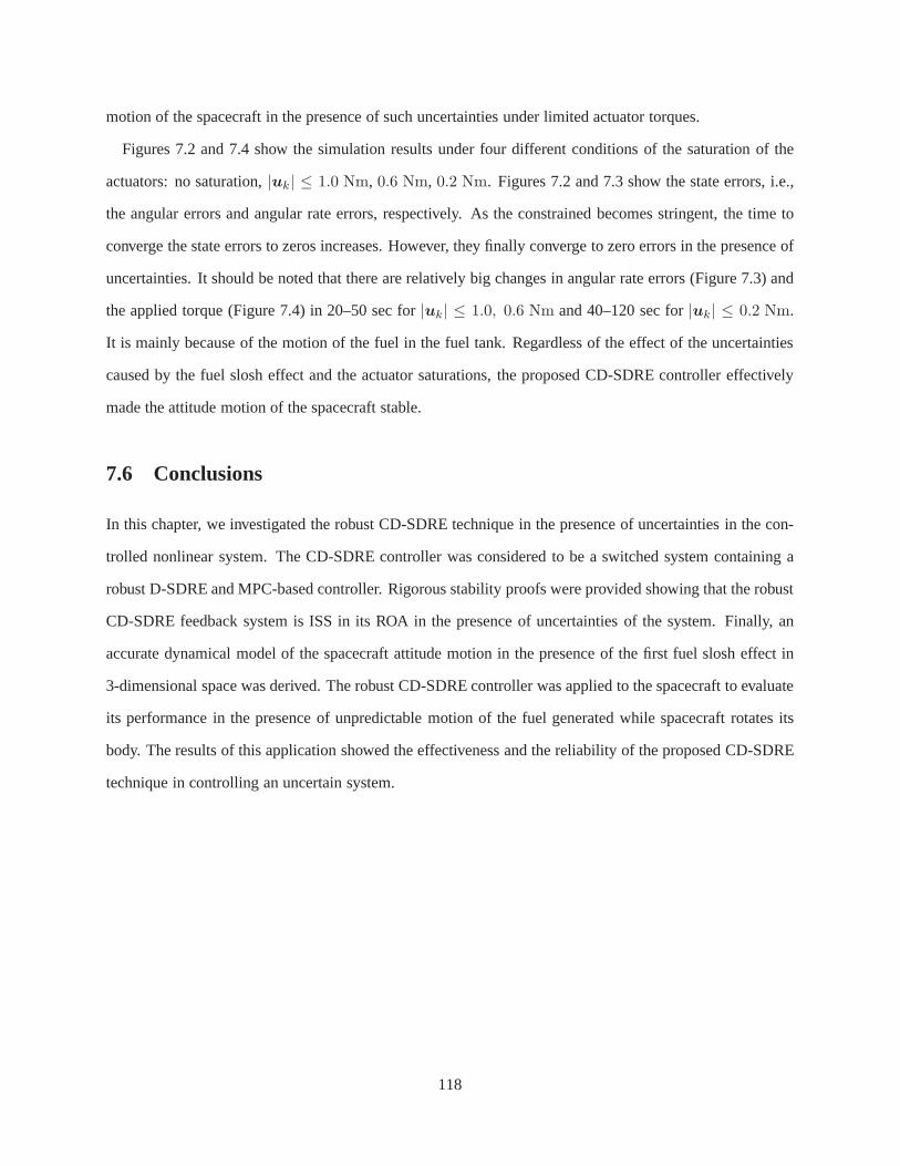
motion of the spacecraft in the presence of such uncertainties under limited actuator torques.
Figures 7.2 and 7.4 show the simulation results under four different conditions of the saturation of the
actuators: no saturation,|uk| ≤ 1.0 Nm, 0.6 Nm, 0.2 Nm. Figures 7.2 and 7.3 show the state errors, i.e.,
the angular errors and angular rate errors, respectively. As the constrained becomes stringent, the time to
converge the state errors to zeros increases. However, theyfinally converge to zero errors in the presence of
uncertainties. It should be noted that there are relativelybig changes in angular rate errors (Figure 7.3) and
the applied torque (Figure 7.4) in 20–50 sec for|uk| ≤ 1.0, 0.6 Nm and 40–120 sec for|uk| ≤ 0.2 Nm.
It is mainly because of the motion of the fuel in the fuel tank.Regardless of the effect of the uncertainties
caused by the fuel slosh effect and the actuator saturations, the proposed CD-SDRE controller effectively
made the attitude motion of the spacecraft stable.
7.6 Conclusions
In this chapter, we investigated the robust CD-SDRE technique in the presence of uncertainties in the con-
trolled nonlinear system. The CD-SDRE controller was considered to be a switched system containing a
robust D-SDRE and MPC-based controller. Rigorous stability proofs were provided showing that the robust
CD-SDRE feedback system is ISS in its ROA in the presence of uncertainties of the system. Finally, an
accurate dynamical model of the spacecraft attitude motionin the presence of the first fuel slosh effect in
3-dimensional space was derived. The robust CD-SDRE controller was applied to the spacecraft to evaluate
its performance in the presence of unpredictable motion of the fuel generated while spacecraft rotates its
body. The results of this application showed the effectiveness and the reliability of the proposed CD-SDRE
technique in controlling an uncertain system.
118

0 50 100 150 200−1
−0.5
0
0.5
φ [r
ad]
0 50 100 150 200−0.5
0
0.5
1
θ [r
ad]
0 50 100 150 200−0.5
0
0.5
1
ψ [r
ad]
Time [s]
No constraintConstraint = 1.0 NmConstraint = 0.6 NmConstraint = 0.2 Nm
Figure 7.2: Time histories of the angular errors of the spacecraft in the presence of different actuatorsaturations (no constraints,±1.0 Nm,±0.6 Nm,±0.2 Nm).
119
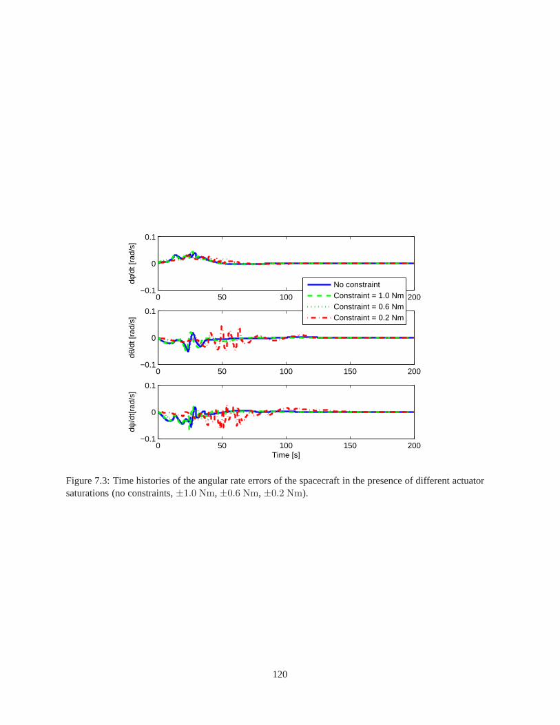
0 50 100 150 200−0.1
0
0.1
dφ/d
t [ra
d/s]
0 50 100 150 200−0.1
0
0.1
dθ/d
t [ra
d/s]
0 50 100 150 200−0.1
0
0.1
dψ/d
t[rad
/s]
Time [s]
No constraintConstraint = 1.0 NmConstraint = 0.6 NmConstraint = 0.2 Nm
Figure 7.3: Time histories of the angular rate errors of the spacecraft in the presence of different actuatorsaturations (no constraints,±1.0 Nm,±0.6 Nm,±0.2 Nm).
120
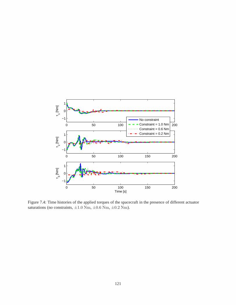
0 50 100 150 200
−1
0
1
τ 1 [Nm
]
0 50 100 150 200
−1
0
1
τ 2 [Nm
]
0 50 100 150 200
−1
0
1
τ 3 [Nm
]
Time [s]
No constraintConstraint = 1.0 NmConstraint = 0.6 NmConstraint = 0.2 Nm
Figure 7.4: Time histories of the applied torques of the spacecraft in the presence of different actuatorsaturations (no constraints,±1.0 Nm,±0.6 Nm,±0.2 Nm).
121
Part III
Filtering Design via D-SDRE
122
Chapter 8
Observer Design via D-SDRE Technique
I N the current and the following chapters, we discuss estimation techniques of the unmeasurable state
parameters in a deterministic or a stochastic nonlinear system, respectively. In this chapter, the observer
based on the D-SDRE technique, called D-SDRE Observer, is investigated in this chapter.
8.1 Discrete-Time State-Dependent Riccati Equation-Based Observer
(D-SDRE Observer)
Suppose that there is a discrete-time deterministic nonlinear system:
xk+1 = f(xk)
yk = h(xk)(8.1)
wherexk ∈ Rn andyk ∈ R
p denote the states and the outputs of the system, respectively.
It is emphasized that the nonlinear dynamical system (8.1) can be reconstructed by using the SDC factor-
ization:
xk+1 = f(xk) = A(xk)xk
yk = h(xk) = C(xk)xk.(8.2)
A one-step procedure is considered for the design of the observer via the D-SDRE technique. Then the
D-SDRE Observer for the nonlinear system can be designed as follows:
xk+1 = A(xk)xk +L(xk)(yk − yk
)
yk = C(xk)xk
(8.3)
123

whereL(xk) ∈ Rn×p is the observer gain, defined as (Song and Grizzle, 1992)
L(xk) := P kC⊤(xk)
(
Rk +C(xk)P kC⊤(xk)
)−1(8.4)
where the symmetric positive definite solutionP k of the D-SDRE can be updated by using the following
equation:
P k+1 = Qk +A(xk)
P k −P kC⊤(xk)
(
C(xk)P kC⊤(xk) +Rk
)−1C(xk)P k
A⊤(xk)
= Qk +A(xk)(
P−1k +C⊤(xk)R
−1k C(xk)
)−1A⊤(xk). (8.5)
It is noted that (8.5) can be rewritten by using the observer gain in (8.4) and the matrix inversion lemma
(Lewis et al., 2012):
P k+1 = Qk +A(xk)
P k −P kC⊤(xk)
(
C(xk)P kC⊤(xk) +Rk
)−1C(xk)P k
A⊤(xk)
= Qk +A(xk)(
P k −L(xk)C(xk)P k
)
A⊤(xk)
= Qk +A(xk)(
I −L(xk)C(xk))
P kA⊤(xk). (8.6)
For the stability analysis of the nonlinear system with the D-SDRE Observer, the error dynamics is
analyzed. The error of the system is defined as follows:
ek := xk − xk (8.7)
wherexk denotes the estimated state of the real statexk by using the D-SDRE Observer.
There are some assumptions for the stability analysis:
Assumption 25 ForA(xk) andC(xk) in (8.3), the following Lipschitz conditions hold for alli ∈ Z≤0:
‖A(xi)−A(xi)‖ ≤ ρA|xi − xi|
‖C(xi)−C(xi)‖ ≤ ρC |xi − xi|(8.8)
for someρA > 0 andρC > 0.
124
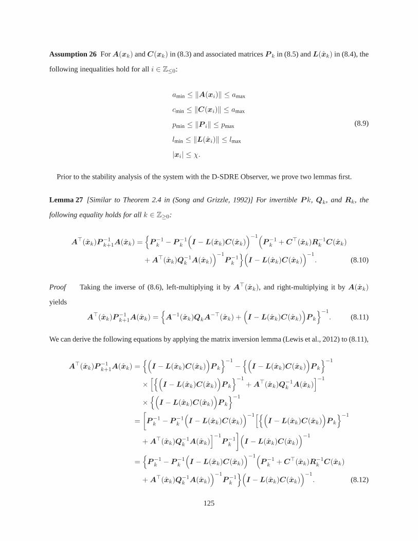
Assumption 26 ForA(xk) andC(xk) in (8.3) and associated matricesP k in (8.5) andL(xk) in (8.4), the
following inequalities hold for alli ∈ Z≤0:
amin ≤ ‖A(xi)‖ ≤ amax
cmin ≤ ‖C(xi)‖ ≤ amax
pmin ≤ ‖P i‖ ≤ pmax
lmin ≤ ‖L(xi)‖ ≤ lmax
|xi| ≤ χ.
(8.9)
Prior to the stability analysis of the system with the D-SDREObserver, we prove two lemmas first.
Lemma 27 [Similar to Theorem 2.4 in (Song and Grizzle, 1992)] For invertible P k, Qk, andRk, the
following equality holds for allk ∈ Z≥0:
A⊤(xk)P−1k+1A(xk) =
P−1k − P−1
k
(
I −L(xk)C(xk))−1(
P−1k +C⊤(xk)R
−1k C(xk)
+A⊤(xk)Q−1k A(xk)
)−1P−1
k
(
I −L(xk)C(xk))−1
. (8.10)
Proof Taking the inverse of (8.6), left-multiplying it byA⊤(xk), and right-multiplying it byA(xk)
yields
A⊤(xk)P−1k+1A(xk) =
A−1(xk)QkA−⊤(xk) +
(
I −L(xk)C(xk))
P k
−1. (8.11)
We can derive the following equations by applying the matrixinversion lemma (Lewis et al., 2012) to (8.11),
A⊤(xk)P−1k+1A(xk) =
(
I −L(xk)C(xk))
P k
−1−(
I −L(xk)C(xk))
P k
−1
×[(
I −L(xk)C(xk))
P k
−1+A⊤(xk)Q
−1k A(xk)
]−1
×(
I −L(xk)C(xk))
P k
−1
=
[
P−1k −P−1
k
(
I −L(xk)C(xk))−1[(
I −L(xk)C(xk))
P k
−1
+A⊤(xk)Q−1k A(xk)
]−1P−1
k
](
I −L(xk)C(xk))−1
=
P−1k − P−1
k
(
I −L(xk)C(xk))−1(
P−1k +C⊤(xk)R
−1k C(xk)
+A⊤(xk)Q−1k A(xk)
)−1P−1
k
(
I −L(xk)C(xk))−1
. (8.12)
125
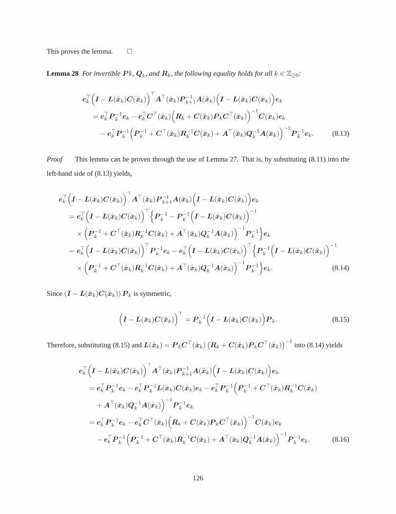
This proves the lemma.
Lemma 28 For invertibleP k, Qk, andRk, the following equality holds for allk ∈ Z≥0:
e⊤k
(
I −L(xk)C(xk))⊤
A⊤(xk)P−1k+1A(xk)
(
I −L(xk)C(xk))
ek
= e⊤k P−1k ek − e⊤k C
⊤(xk)(
Rk +C(xk)P kC⊤(xk)
)−1C(xk)ek
− e⊤k P−1k
(
P−1k +C⊤(xk)R
−1k C(xk) +A⊤(xk)Q
−1k A(xk)
)−1P−1
k ek. (8.13)
Proof This lemma can be proven through the use of Lemma 27. That is, by substituting (8.11) into the
left-hand side of (8.13) yields,
e⊤k
(
I −L(xk)C(xk))⊤
A⊤(xk)P−1k+1A(xk)
(
I −L(xk)C(xk))
ek
= e⊤k
(
I −L(xk)C(xk))⊤
P−1k − P−1
k
(
I −L(xk)C(xk))−1
×(
P−1k +C⊤(xk)R
−1k C(xk) +A⊤(xk)Q
−1k A(xk)
)−1P−1
k
ek
= e⊤k
(
I −L(xk)C(xk))⊤
P−1k ek − e⊤k
(
I −L(xk)C(xk))⊤
P−1k
(
I −L(xk)C(xk))−1
×(
P−1k +C⊤(xk)R
−1k C(xk) +A⊤(xk)Q
−1k A(xk)
)−1P−1
k
ek. (8.14)
Since(I −L(xk)C(xk))P k is symmetric,
(
I −L(xk)C(xk))⊤
= P−1k
(
I −L(xk)C(xk))
P k. (8.15)
Therefore, substituting (8.15) andL(xk) = P kC⊤(xk)
(Rk +C(xk)P kC
⊤(xk))−1
into (8.14) yields
e⊤k
(
I −L(xk)C(xk))⊤
A⊤(xk)P−1k+1A(xk)
(
I −L(xk)C(xk))
ek
= e⊤k P−1k ek − e⊤k P
−1k L(xk)C(xk)ek − e⊤k P
−1k
(
P−1k +C⊤(xk)R
−1k C(xk)
+A⊤(xk)Q−1k A(xk)
)−1P−1
k ek
= e⊤k P−1k ek − e⊤k C
⊤(xk)(
Rk +C(xk)P kC⊤(xk)
)−1C(xk)ek
− e⊤k P−1k
(
P−1k +C⊤(xk)R
−1k C(xk) +A⊤(xk)Q
−1k A(xk)
)−1P−1
k ek. (8.16)
126
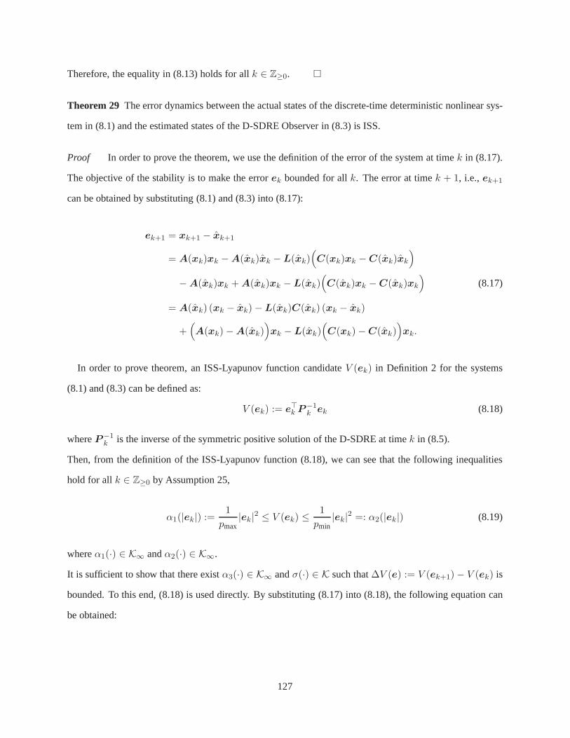
Therefore, the equality in (8.13) holds for allk ∈ Z≥0.
Theorem 29 The error dynamics between the actual states of the discrete-time deterministic nonlinear sys-
tem in (8.1) and the estimated states of the D-SDRE Observer in (8.3) is ISS.
Proof In order to prove the theorem, we use the definition of the error of the system at timek in (8.17).
The objective of the stability is to make the errorek bounded for allk. The error at timek + 1, i.e.,ek+1
can be obtained by substituting (8.1) and (8.3) into (8.17):
ek+1 = xk+1 − xk+1
= A(xk)xk −A(xk)xk −L(xk)(
C(xk)xk −C(xk)xk
)
−A(xk)xk +A(xk)xk −L(xk)(
C(xk)xk −C(xk)xk
)
(8.17)
= A(xk) (xk − xk)−L(xk)C(xk) (xk − xk)
+(
A(xk)−A(xk))
xk −L(xk)(
C(xk)−C(xk))
xk.
In order to prove theorem, an ISS-Lyapunov function candidate V (ek) in Definition 2 for the systems
(8.1) and (8.3) can be defined as:
V (ek) := e⊤k P−1k ek (8.18)
whereP−1k is the inverse of the symmetric positive solution of the D-SDRE at timek in (8.5).
Then, from the definition of the ISS-Lyapunov function (8.18), we can see that the following inequalities
hold for allk ∈ Z≥0 by Assumption 25,
α1(|ek|) :=1
pmax|ek|2 ≤ V (ek) ≤
1
pmin|ek|2 =: α2(|ek|) (8.19)
whereα1(·) ∈ K∞ andα2(·) ∈ K∞.
It is sufficient to show that there existα3(·) ∈ K∞ andσ(·) ∈ K such that∆V (e) := V (ek+1)− V (ek) is
bounded. To this end, (8.18) is used directly. By substituting (8.17) into (8.18), the following equation can
be obtained:
127
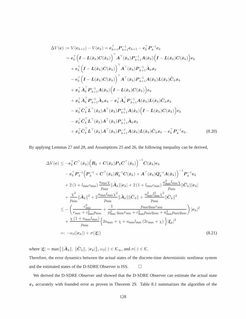
∆V (e) := V (ek+1)− V (ek) = e⊤k+1P−1k+1ek+1 − e⊤k P
−1k ek
= e⊤k
(
I −L(xk)C(xk))⊤
A⊤(xk)P−1k+1A(xk)
(
I −L(xk)C(xk))
ek
+ e⊤k
(
I −L(xk)C(xk))⊤
A⊤(xk)P−1k+1Akxk
− e⊤k
(
I −L(xk)C(xk))⊤
A⊤(xk)P−1k+1A(xk)L(xk)Ckxk
+ x⊤k A
⊤k P
−1k+1A(xk)
(
I −L(xk)C(xk))
ek
+ x⊤k A
⊤k P
−1k+1Akxk − x⊤
k A⊤k P
−1k+1A(xk)L(xk)Ckxk
− x⊤k C
⊤k L
⊤(xk)A⊤(xk)P
−1k+1A(xk)
(
I −L(xk)C(xk))
ek
− x⊤k C
⊤k L
⊤(xk)A⊤(xk)P
−1k+1Akxk
+ x⊤k C
⊤k L
⊤(xk)A⊤(xk)P
−1k+1A(xk)L(xk)Ckxk − e⊤k P
−1k ek. (8.20)
By applying Lemmas 27 and 28, and Assumptions 25 and 26, the following inequality can be derived,
∆V (e) ≤ −e⊤k C⊤(xk)(
Rk +C(xk)P kC⊤(xk)
)−1C(xk)ek
− e⊤k P−1k
(
P−1k +C⊤(xk)R
−1k C(xk) +A⊤(xk)Q
−1k A(xk)
)−1P−1
k ek
+ 2 (1 + lmaxcmax)amaxχ
pmin‖Ak‖|ek|+ 2 (1 + lmaxcmax)
a2maxlmaxχ
pmin‖Ck‖|ek|
+χ2
pmin‖Ak‖2 + 2
amaxlmaxχ2
pmin‖Ak‖‖Ck‖+
a2maxl2maxχ
2
pmin‖Ck‖2
≤ −(
c2min
rmax+ c2maxpmax+
1
p2max
pminqminrmin
qminrmin + c2maxpminqmin + a2maxpminqmin
)
|ek|2
+χ (1 + amaxlmax)
pmin
2amax+ χ+ amaxlmax(2cmax+ χ)
|ξk|2
=: −α3(|ek|) + σ(|ξ|) (8.21)
where|ξ| = max‖Ak‖, ‖Ck‖, |ek|
, α3(·) ∈ K∞, andσ(·) ∈ K.
Therefore, the error dynamics between the actual states of the discrete-time deterministic nonlinear system
and the estimated states of the D-SDRE Observer is ISS.
We derived the D-SDRE Observer and showed that the D-SDRE Observer can estimate the actual state
xk accurately with founded error as proven in Theorem 29. Table8.1 summarizes the algorithm of the
128
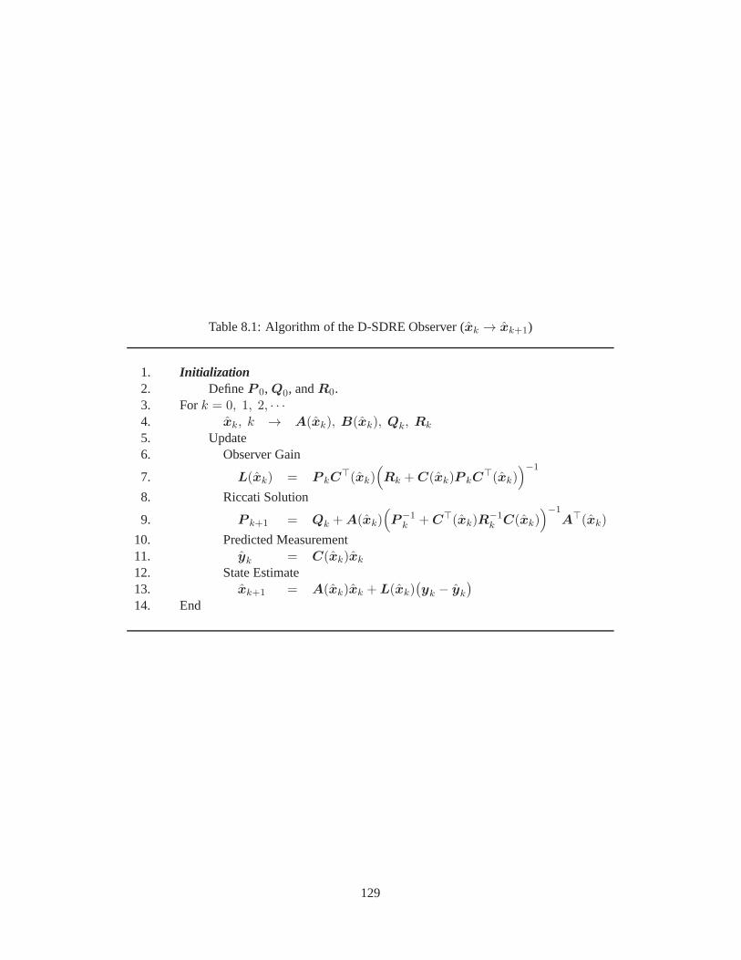
Table 8.1: Algorithm of the D-SDRE Observer (xk → xk+1)
1. Initialization2. DefineP 0, Q0, andR0.3. Fork = 0, 1, 2, · · ·4. xk, k → A(xk), B(xk), Qk, Rk
5. Update6. Observer Gain
7. L(xk) = P kC⊤(xk)
(
Rk +C(xk)P kC⊤(xk)
)−1
8. Riccati Solution
9. P k+1 = Qk +A(xk)(
P−1k +C⊤(xk)R
−1k C(xk)
)−1A⊤(xk)
10. Predicted Measurement11. yk = C(xk)xk
12. State Estimate13. xk+1 = A(xk)xk +L(xk)
(yk − yk
)
14. End
129

D-SDRE Observer.
In the next section, we evaluate the performance of the D-SDRE Observer by using a chaotic dynamical
system.
8.2 Numerical Validation
Based on the algorithm of the D-SDRE Observer in Table 8.1, weevaluate its performance by using the
Lorenz attractor (Lorenz, 1963). The Lorenz attractor, a nonlinear deterministic 3-dimensional system, is
a simplified mathematical model for atmospheric convection, which has chaotic solutions for certain initial
conditions and parameters in the equation. It has the following form:
x = σ(y − x)
y = x(ρ− z)− y (8.22)
z = xy − βz
wherex, y, andz denote the states of the system andσ, ρ, andβ design parameters.
In order to apply the D-SDRE Observer, (8.22) needs to be discretized. DefiningT as a sampling time of
the system yields the discretization of the states:x =xk+1−xk
T , y =yk+1−yk
T , andz =zk+1−zk
T . Substituting
theses equations into (8.22) yields the discrete-time Lorenz attractor as
xk+1 = xk + Tσ(yk − xk)
yk+1 = yk + Txk(ρ− zk)− Tyk (8.23)
zk+1 = zk + Txkyk − Tβzk.
These equations can be expressed in a compact form by using a matrix structure as follows:
xk+1
yk+1
zk+1
︸ ︷︷ ︸
=:xk+1
=
1− Tσ Tσ 0
Tρ 1− T −Txk0 Txk 1− Tβ
︸ ︷︷ ︸
=:A(xk)
xk
yk
zk
︸ ︷︷ ︸
=:xk
. (8.24)
130
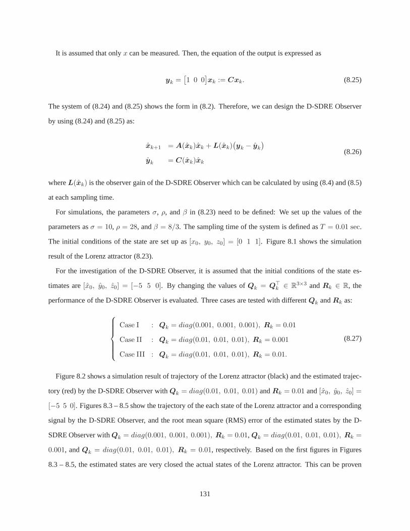
It is assumed that onlyx can be measured. Then, the equation of the output is expressed as
yk =[1 0 0
]xk := Cxk. (8.25)
The system of (8.24) and (8.25) shows the form in (8.2). Therefore, we can design the D-SDRE Observer
by using (8.24) and (8.25) as:
xk+1 = A(xk)xk +L(xk)(yk − yk
)
yk = C(xk)xk
(8.26)
whereL(xk) is the observer gain of the D-SDRE Observer which can be calculated by using (8.4) and (8.5)
at each sampling time.
For simulations, the parametersσ, ρ, andβ in (8.23) need to be defined: We set up the values of the
parameters asσ = 10, ρ = 28, andβ = 8/3. The sampling time of the system is defined asT = 0.01 sec.
The initial conditions of the state are set up as[x0, y0, z0] = [0 1 1]. Figure 8.1 shows the simulation
result of the Lorenz attractor (8.23).
For the investigation of the D-SDRE Observer, it is assumed that the initial conditions of the state es-
timates are[x0, y0, z0] = [−5 5 0]. By changing the values ofQk = Q⊤k ∈ R
3×3 andRk ∈ R, the
performance of the D-SDRE Observer is evaluated. Three cases are tested with differentQk andRk as:
Case I : Qk = diag(0.001, 0.001, 0.001), Rk = 0.01
Case II : Qk = diag(0.01, 0.01, 0.01), Rk = 0.001
Case III : Qk = diag(0.01, 0.01, 0.01), Rk = 0.01.
(8.27)
Figure 8.2 shows a simulation result of trajectory of the Lorenz attractor (black) and the estimated trajec-
tory (red) by the D-SDRE Observer withQk = diag(0.01, 0.01, 0.01) andRk = 0.01 and[x0, y0, z0] =
[−5 5 0]. Figures 8.3 – 8.5 show the trajectory of the each state of theLorenz attractor and a corresponding
signal by the D-SDRE Observer, and the root mean square (RMS)error of the estimated states by the D-
SDRE Observer withQk = diag(0.001, 0.001, 0.001), Rk = 0.01, Qk = diag(0.01, 0.01, 0.01), Rk =
0.001, andQk = diag(0.01, 0.01, 0.01), Rk = 0.01, respectively. Based on the first figures in Figures
8.3 – 8.5, the estimated states are very closed the actual states of the Lorenz attractor. This can be proven
131
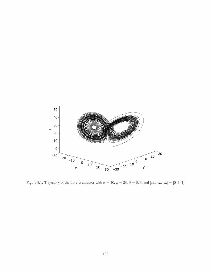
−30−20
−100
1020
30 −30−20
−100
1020
30
0
10
20
30
40
50
yx
z
Figure 8.1: Trajectory of the Lorenz attractor withσ = 10, ρ = 28, β = 8/3, and[x0, y0, z0] = [0 1 1]
132
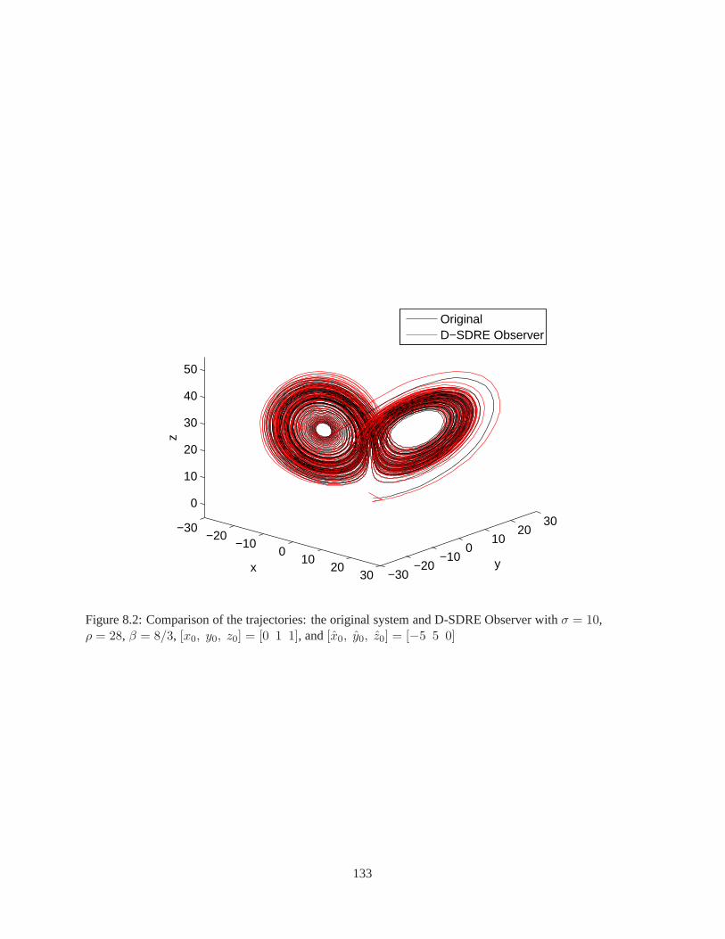
−30−20
−100
1020
30 −30−20
−100
1020
30
0
10
20
30
40
50
yx
z
OriginalD−SDRE Observer
Figure 8.2: Comparison of the trajectories: the original system and D-SDRE Observer withσ = 10,ρ = 28, β = 8/3, [x0, y0, z0] = [0 1 1], and[x0, y0, z0] = [−5 5 0]
133

more clearly by using the second figures in Figures 8.3 – 8.5. Due to the mismatches of the initial condi-
tions between the actual state values and the the D-SDRE Observer, the RMS errors have large values at
the beginning of the simulations (0–1 sec). However, after the effect of the initial mismatches, the average
values of the RMS errors converge to certain values. The results show that the estimation of the states by
using the D-SDRE Observer is reliable regardless of the values ofQk andRk.
8.3 Conclusion
In this chapter, we introduced the D-SDRE Observer, based onthe D-SDRE technique introduced in the
Chapter 5. We have investigated condition of the error between the actual state of the nonlinear deterministic
system and the estimated one by using the D-SDRE Observer andhave proven that the error dynamics is
ISS. We applied the D-SDRE Observer to the Lorenz attractor to estimate the states and the results showed
that the Observer is reliable regardless of the values of theQk andRk.
However, it should be noted that the D-SDRE Observer was designed for thedeterministicsystem. There-
fore, we should investigate the case where there are stochastic terms in the dynamical systems, which is the
topic for the next chapter.
134
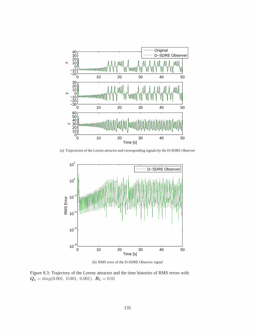
0 10 20 30 40 50−20−10
010203040
x
0 10 20 30 40 50−30−20−10
0102030
y
0 10 20 30 40 500
102030405060
z
Time [s]
OriginalD−SDRE Observer
(a) Trajectories of the Lorenz attractor and correspondingsignals by the D-SDRE Observer
0 10 20 30 40 5010
−8
10−6
10−4
10−2
100
102
Time [s]
RM
S E
rror
D−SDRE Observer
(b) RMS error of the D-SDRE Observer signal
Figure 8.3: Trajectory of the Lorenz attractor and the time histories of RMS errors withQk = diag(0.001, 0.001, 0.001), Rk = 0.01
135
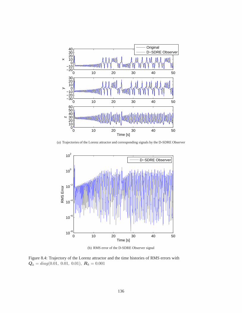
0 10 20 30 40 50−20−10
010203040
x
0 10 20 30 40 50−30−20−10
0102030
y
0 10 20 30 40 500
102030405060
z
Time [s]
OriginalD−SDRE Observer
(a) Trajectories of the Lorenz attractor and correspondingsignals by the D-SDRE Observer
0 10 20 30 40 5010
−8
10−6
10−4
10−2
100
102
Time [s]
RM
S E
rror
D−SDRE Observer
(b) RMS error of the D-SDRE Observer signal
Figure 8.4: Trajectory of the Lorenz attractor and the time histories of RMS errors withQk = diag(0.01, 0.01, 0.01), Rk = 0.001
136
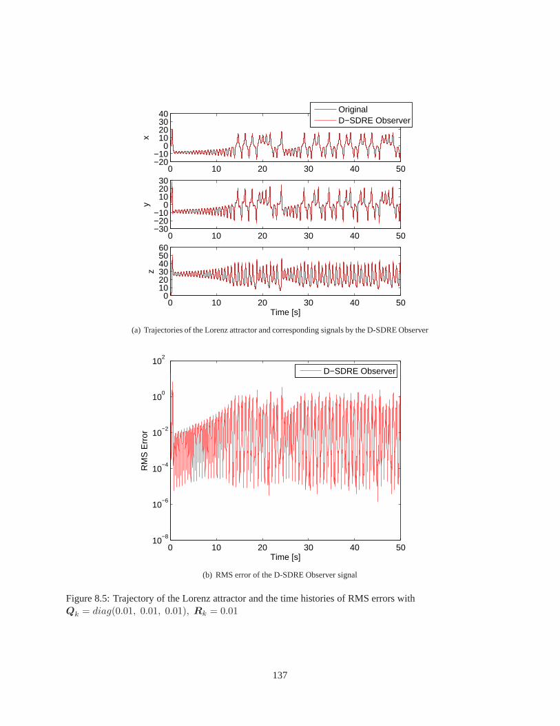
0 10 20 30 40 50−20−10
010203040
x
0 10 20 30 40 50−30−20−10
0102030
y
0 10 20 30 40 500
102030405060
z
Time [s]
OriginalD−SDRE Observer
(a) Trajectories of the Lorenz attractor and correspondingsignals by the D-SDRE Observer
0 10 20 30 40 5010
−8
10−6
10−4
10−2
100
102
Time [s]
RM
S E
rror
D−SDRE Observer
(b) RMS error of the D-SDRE Observer signal
Figure 8.5: Trajectory of the Lorenz attractor and the time histories of RMS errors withQk = diag(0.01, 0.01, 0.01), Rk = 0.01
137

Chapter 9
The D-SDRE-Based Filter Design
9.1 Introduction
TWO filtering techniques are investigated by using the discrete-time state-dependent Riccati equation
(D-SDRE) technique. Detailed derivation of the D-SDRE-based filter (D-SDREF) is provided under
the assumption of Gaussian noises and the stability condition of the error signal between the measured signal
and the estimated signals is proven to be input-to-state stable. For the non-Gaussian distributed noises, we
propose a filter by combining the D-SDREF and the particle filter (PF), named the combined D-SDRE/PF.
Two algorithms for the filtering techniques are provided. Several filtering techniques are compared with
challenging numerical examples to show the reliability andefficacy of the proposed D-SDREF and the
combined D-SDRE/particle filter.
The rest of the chapter is organized as follows: The D-SDREF is derived in Section 9.2. Its stability
condition is rigorously investigated in Section 9.3. The combined D-SDRE/PF is introduced in Section
9.4. In Section 9.5, the proposed D-SDREF and the combined D-SDRE/PF are evaluated by using two
challenging examples. Finally, concluding remarks are made in Section 9.6.
9.2 Discrete-Time State-Dependent Riccati Equation-Based Filter
(D-SDREF)
In this section, we derive the D-SDREF technique. Consider adiscrete-time nonlinear stochastic system:
xk = f(xk−1,wk−1) = A(xk−1)xk−1 +Gk−1ωk−1
yk = h(xk,νk) = C(xk)xk + Γkνk
(9.1)
138
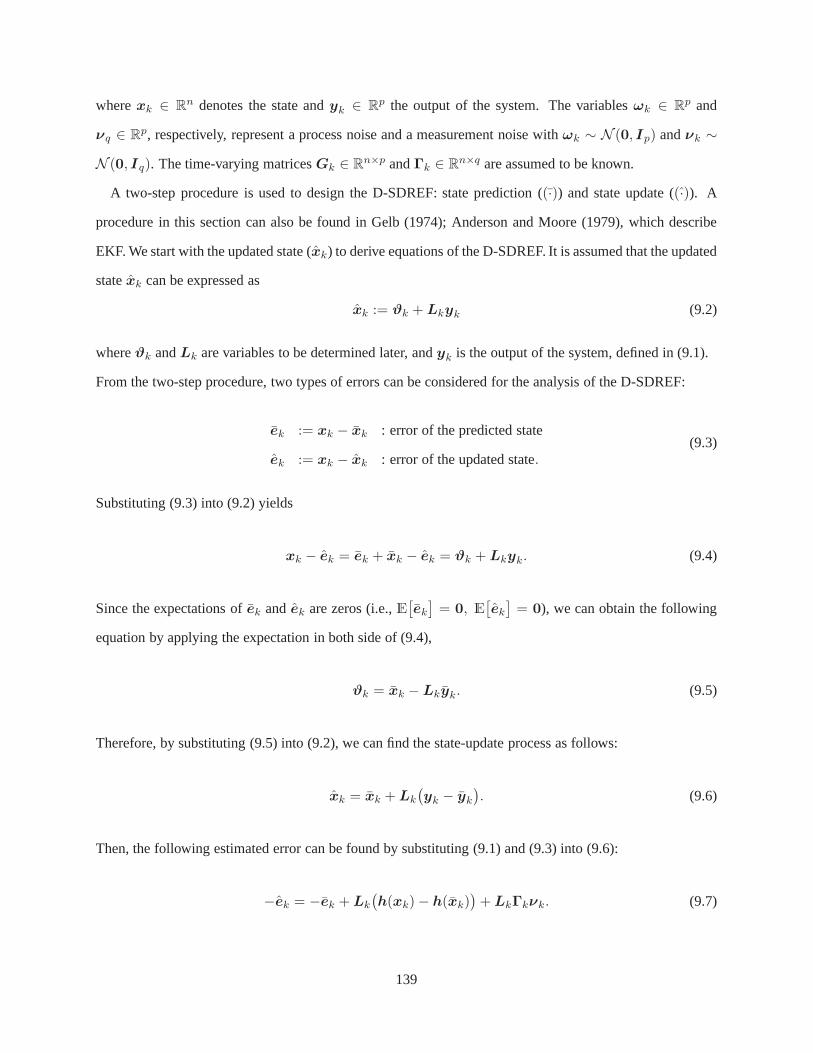
wherexk ∈ Rn denotes the state andyk ∈ R
p the output of the system. The variablesωk ∈ Rp and
νq ∈ Rp, respectively, represent a process noise and a measurementnoise withωk ∼ N (0, Ip) andνk ∼
N (0, Iq). The time-varying matricesGk ∈ Rn×p andΓk ∈ R
n×q are assumed to be known.
A two-step procedure is used to design the D-SDREF: state prediction ((·)) and state update ((·)). A
procedure in this section can also be found in Gelb (1974); Anderson and Moore (1979), which describe
EKF. We start with the updated state (xk) to derive equations of the D-SDREF. It is assumed that the updated
statexk can be expressed as
xk := ϑk +Lkyk (9.2)
whereϑk andLk are variables to be determined later, andyk is the output of the system, defined in (9.1).
From the two-step procedure, two types of errors can be considered for the analysis of the D-SDREF:
ek := xk − xk : error of the predicted state
ek := xk − xk : error of the updated state.(9.3)
Substituting (9.3) into (9.2) yields
xk − ek = ek + xk − ek = ϑk +Lkyk. (9.4)
Since the expectations ofek andek are zeros (i.e.,E[ek]= 0, E
[ek]= 0), we can obtain the following
equation by applying the expectation in both side of (9.4),
ϑk = xk −Lkyk. (9.5)
Therefore, by substituting (9.5) into (9.2), we can find the state-update process as follows:
xk = xk +Lk
(yk − yk
). (9.6)
Then, the following estimated error can be found by substituting (9.1) and (9.3) into (9.6):
−ek = −ek +Lk
(h(xk)− h(xk)
)+LkΓkνk. (9.7)
139
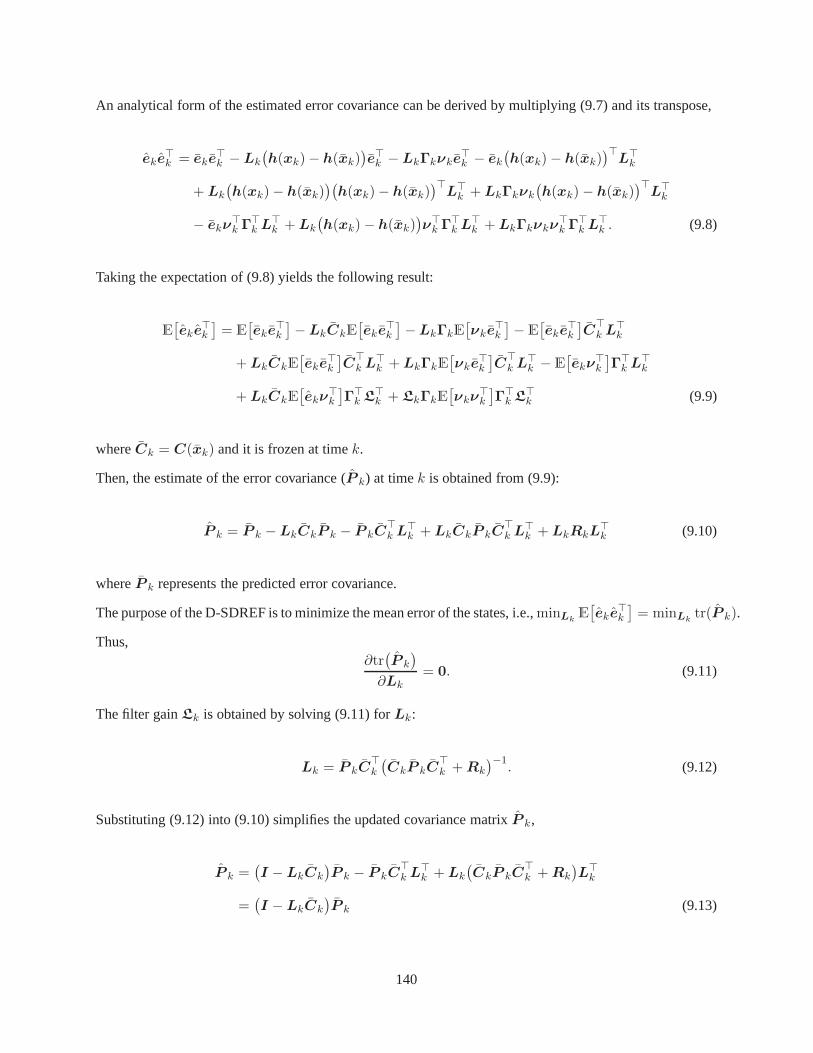
An analytical form of the estimated error covariance can be derived by multiplying (9.7) and its transpose,
eke⊤k = eke
⊤k −Lk
(h(xk)− h(xk)
)e⊤k −LkΓkνke
⊤k − ek
(h(xk)− h(xk)
)⊤L⊤
k
+Lk
(h(xk)− h(xk)
)(h(xk)− h(xk)
)⊤L⊤
k +LkΓkνk
(h(xk)− h(xk)
)⊤L⊤
k
− ekν⊤k Γ
⊤k L
⊤k +Lk
(h(xk)− h(xk)
)ν⊤k Γ
⊤k L
⊤k +LkΓkνkν
⊤k Γ
⊤k L
⊤k . (9.8)
Taking the expectation of (9.8) yields the following result:
E[eke
⊤k
]= E
[eke
⊤k
]−LkCkE
[eke
⊤k
]−LkΓkE
[νke
⊤k
]− E
[eke
⊤k
]C
⊤k L
⊤k
+LkCkE[eke
⊤k
]C
⊤k L
⊤k +LkΓkE
[νke
⊤k
]C
⊤k L
⊤k − E
[ekν
⊤k
]Γ⊤k L
⊤k
+LkCkE[ekν
⊤k
]Γ⊤k L
⊤k +LkΓkE
[νkν
⊤k
]Γ⊤k L
⊤k (9.9)
whereCk = C(xk) and it is frozen at timek.
Then, the estimate of the error covariance (P k) at timek is obtained from (9.9):
P k = P k −LkCkP k − P kC⊤k L
⊤k +LkCkP kC
⊤k L
⊤k +LkRkL
⊤k (9.10)
whereP k represents the predicted error covariance.
The purpose of the D-SDREF is to minimize the mean error of thestates, i.e.,minLkE[eke
⊤k
]= minLk
tr(P k).
Thus,∂tr(P k
)
∂Lk= 0. (9.11)
The filter gainLk is obtained by solving (9.11) forLk:
Lk = P kC⊤k
(CkP kC
⊤k +Rk
)−1. (9.12)
Substituting (9.12) into (9.10) simplifies the updated covariance matrixP k,
P k =(I −LkCk
)P k − P kC
⊤k L
⊤k +Lk
(CkP kC
⊤k +Rk
)L⊤
k
=(I −LkCk
)P k (9.13)
140

which is known as the Joseph algorithm (Gelb, 1974; Stengel,1994) for a linearized system.
The predicted error covariance matrixP k can be obtained directly from its definition:
P k = cov[ek]= Ak−1P k−1A
⊤k−1 +Qk−1 (9.14)
whereAk−1 := A(xk−1).
Table 9.1 summarizes the algorithm of the D-SDREF discussedso far.
Based on the derivation of the D-SDREF, its error bounds are investigated in the following section.
9.3 Error Bounds for the D-SDREF
In this section, we want to show that the errors between the actual states and the estimated ones by using the
D-SDREF are bounded in the presence of disturbances sourcessuch as process noise, measurement noise,
model uncertainties, etc. Prior to that, we consider the following assumptions of the states and the values of
the matrices in the dynamical model (9.1) and the filtering model in Table 30.
Assumption 30 Given the nonlinear stochastic system (9.1), the followingassumptions hold for allk ∈
Z≥0:
‖A(xk)−A(xk)‖ ≤ ρA|xk − xk|
‖C(xk)−C(xk)‖ ≤ ρC |xk − xk|
amin ≤ ‖A(xk)‖ ≤ amax
cmin ≤ ‖C(xk)‖ ≤ cmax
pmin ≤ ‖P k‖ ≤ pmax
lmin ≤ ‖L(xk)‖ ≤ lmax
|xk| ≤ χ
(9.15)
for someρA > 0 andρC > 0.
The first two in Assumption 30 show the Lipschitz condition and the last one shows that the states of the
system are bounded.
Prior to the stability analysis of the system with the D-SDREF, we discuss two useful lemmas first that will
be used to prove the stability of the error bounds.
141

Table 9.1: Algorithm of the D-SDREF
Initialization (k = 0)DefineP 0, Q0, andR0.
Fork = 1, 2, 3, · · ·Prediction (xk−1, P k−1,→ xk, P k)
Predicted State
xk = f(xk−1) = A(xk−1)xk−1 = Ak−1xk−1
Predicted Measurement
yk = h(xk) = C(xk)xk = Ckxk
Predicted Error Covariance
P k = Ak−1P k−1A⊤k−1 +Qk−1
Update (xk, P k → xk, P k)
Filter Gain
Lk = P kC⊤k
(CkP kC
⊤k +Rk
)−1
State Estimate
xk = xk +Lk
(yk − yk
)
Error Covariance Estimate
P k =(I −LkCk
)P k
End
142
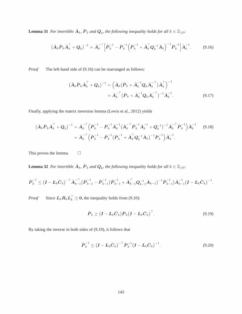
Lemma 31 For invertibleAk, P k andQk, the following inequality holds for allk ∈ Z≥0:
(AkP kA
⊤k +Qk
)−1= A
−⊤k
[
P−1k − P
−1k
(
P−1k + A
⊤k Q
−1k Ak
)−1P
−1k
]
A−1k . (9.16)
Proof The left-hand side of (9.16) can be rearranged as follows:
(AkP kA
⊤k +Qk
)−1=(
Ak
(P k + A
−1k QkA
−⊤k
)A
⊤k
)−1
= A−⊤k
(P k + A
−1k QkA
−⊤k
)−1A
−1k . (9.17)
Finally, applying the matrix inversion lemma (Lewis et al.,2012) yields
(AkP kA
⊤k +Qk
)−1= A
−⊤k
(
P−1k − P
−1k A
−1k
(A
−⊤k P
−1k A
−1k +Q−1
k
)−1A
−⊤k P
−1k
)
A−1k (9.18)
= A−⊤k
(
P−1k − P
−1k
(P
−1k + A
⊤k Q
−1k Ak
)−1P
−1k
)
A−1k .
This proves the lemma.
Lemma 32 For invertibleAk, P k andQk, the following inequality holds for allk ∈ Z≥0:
P−1k ≤
(I −LkCk
)−⊤A
−⊤k−1
(P
−1k−1 − P
−1k−1
(P
−1k−1 + A
⊤k−1Q
−1k−1Ak−1
)−1P
−1k−1
)A
−1k−1
(I −LkCk
)−1.
Proof SinceLkRkL⊤k ≥ 0, the inequality holds from (9.10):
P k ≥(I −LkCk
)P k
(I −LkCk
)⊤. (9.19)
By taking the inverse in both sides of (9.19), it follows that
P−1k ≤
(I −LkCk
)−⊤P
−1k
(I −LkCk
)−1. (9.20)
143
The lemma can be proven by the definition ofP k and Lemma 31:
P−1k ≤
(I −LkCk
)−⊤(
Ak−1P k−1Ak−1 +Qk−1
)−1(I −LkCk
)−1
=(I −LkCk
)−⊤A
−⊤k−1
(
P−1k−1 − P
−1k−1
(P
−1k−1 + A
⊤k−1Q
−1k−1Ak−1
)−1P
−1k−1
)
× A−1k−1
(I −LkCk
)−1. (9.21)
Therefore, the inequality holds for allk ∈ Z≥0.
Theorem 33 The error dynamics between the actual states of the discrete-time stochastic nonlinear system
(9.1) and the estimated states of the D-SDREF in Table 9.1 is ISS.
Proof In order to prove the stable error bound on states, we recall the definition of the state error in (9.3).
Then, substituting (9.1) and (9.6) into (9.3) yields
ek = xk − xk
= Ak−1xk−1 +Gk−1ωk−1 − xk −Lk
(yk − yk
)
= Ak−1
(xk−1 − xk−1
)−LkCkek +
(Ak−1 − Ak−1
)xk−1 +Gk−1ωk−1 −LkΓkνk
= Ak−1ek−1 −LkCkAk−1ek−1 −LkCkGk−1ωk−1 + Ak−1xk−1
+Gk−1ωk−1 −LkΓkνk (9.22)
whereAk−1 := Ak−1 − Ak−1.
For the proof, we define an ISS-Lyapunov function candidate as follows:
V (ek) := e⊤k P−1k ek (9.23)
whereP−1k is the inverse of the updated error covariance of the system.
144

By substituting (9.22) into (9.23), the following derivation can be obtained:
V (ek) =((
I −LkCk
)Ak−1ek−1 + Ak−1xk−1 +
(I −LkCk
)Gk−1ωk−1 −LkΓkνk
)⊤P
−1k
×((
I −LkCk
)Ak−1ek−1 + Ak−1xk−1 +
(I −LkCk
)Gk−1ωk−1 −LkΓkνk
)
= e⊤k−1
((I −LkCk
)Ak−1
)⊤P
−1k
((I −LkCk
)Ak−1
)
ek−1
+ e⊤k−1
((I −LkCk
)Ak−1
)⊤P
−1k Ak−1xk−1
+ e⊤k−1
((I −LkCk
)Ak−1
)⊤P
−1k
(I −LkCk
)Gk−1ωk−1
− e⊤k−1
((I −LkCk
)Ak−1
)⊤P
−1k LkΓkνk
+ x⊤k−1A
⊤k−1P
−1k
((I −LkCk
)Ak−1
)
ek−1 + x⊤k−1A
⊤k−1P
−1k Ak−1xk−1
+ x⊤k−1A
⊤k−1P
−1k
(I −LkCk
)Gk−1ωk−1 − x⊤
k−1A⊤k−1P
−1k LkΓkνk
+ω⊤k−1G
⊤k−1
(I −LkCk
)⊤P
−1k
((I −LkCk
)Ak−1
)
ek−1
+ω⊤k−1G
⊤k−1
(I −LkCk
)⊤P
−1k Ak−1xk−1
+ω⊤k−1G
⊤k−1
(I −LkCk
)⊤P
−1k
(I −LkCk
)Gk−1ωk−1
−ω⊤k−1G
⊤k−1
(I −LkCk
)⊤P
−1k LkΓkνk
− νkΓ⊤k L
⊤k P
−1k
((I −LkCk
)Ak−1
)
ek−1 − νkΓ⊤k L
⊤k P
−1k Ak−1xk−1
− νkΓ⊤k L
⊤k P
−1k
(I −LkCk
)Gk−1ωk−1 + νkΓ
⊤k L
⊤k P
−1k LkΓkνk. (9.24)
145
Applying Lemma 32 into (9.24) yields the following inequality:
V (e) := V (ek)− V (ek−1)
≤ −e⊤k−1P−1k−1
(
P−1k−1 + A
⊤k−1Q
−1k−1Ak−1
)−1P
−1k−1ek−1
+2(1 + lmaxcmax)amaxχ
pmin‖Ak−1‖|ek−1|+
2(1 + lmaxcmax)2amax
pmin‖Gk−1‖|ek−1|
+2(1 + lmaxcmax)amaxlmax
pmin‖Γk‖|ek−1|+
χ2
pmin‖Ak−1‖2
+2(1 + lmaxcmax)χ
pmin‖Ak−1‖‖Gk−1‖+
2lmaxχ
pmin‖Ak−1‖‖Γk‖
+(1 + lmaxcmax)
2
pmin‖Gk−1‖2 +
2(1 + lmaxcmax)lmax
pmin‖Gk−1‖‖Γk‖+
l2max
pmin‖Γk‖2
≤ − pminqmin
p2max
(qmin + pmina2max
) |ek|2 +1
pmin
(
(χ+ lmax)2 + 2(1 + lmaxcmax)(amax + 1)(χ + lmax)
+ (1 + lmaxcmax)2(2amax + 1)
)
|ξk|2
=: −α3(|ek|) + σ(|ξk|) (9.25)
where|ξk| := max‖Ak‖, ‖Gk‖, ‖Γk‖, |ek|
.
Therefore, the system is ISS by Definitions 1 and 2.
In this section, we derived analytical forms of the D-SDREF and showed the stability condition between
the measured signal and the estimated one under the assumption of Gaussian noises. In the next section, we
investigate a new filter to improve the performance of the filter in the presence of non-Gaussian noises.
9.4 Combined D-SDRE/Particle Filter
In this section, we want to extend the D-SDREF to the case where the noises in a system follow non-
Gaussian distribution. It should be noted that the D-SDREF was developed based on the assumption of
Gaussian distribution. We propose a new filtering techniqueby combining the D-SDREF with particle filters
(PF), named the combined D-SDRE/PF. Prior to discussing thebenefits of D-SDRE/PF, we summarize the
advantages of the proposed D-SDREF compared to other filtering techniques discussed:
1. D-SDREF propagates the states by using the full nonlinearmodel (more accurate propagation).
2. The full nonlinear model is factorized by using the SDC factorization without explicit calculation of
146
Jacobians or Hessians.
3. The computational burden is less than EKF (no linearization), UKF (no sigma points), MHE (no
horizon of measurements), or PF (no samples).
However, it should be noted that the D-SDREF was designed under the assumption of the Gaussian noises.
Therefore, the D-SDREF is not suitable for a system with non-Gaussian noises. Among filtering techniques
that can handle non-Gaussian noises, PF shows its reliability as well as simplicity to be implemented in
a system. It is interesting to note that PF is one of the filtering techniques that can handle Gaussian/non-
Gaussian noises. The advantages of the PF are as follows (Rawlings and Mayne, 2009):
1. PF uses the full nonlinear model to propagate the samples.
2. The PF sampled density can represent a general conditional density.
3. PF is simple to program and executes quickly for small sample sizes.
However, PF has weaknesses to be operated alone in a system. For examples, the performance of PF
becomes worse as the state dimensions increases. It is also sensitive to unmodeled disturbances (Rawlings
and Mayne, 2009). There have been studies to investigate thebenefits of filtering techniques by combining
them with PF not only to overcome their weaknesses but also totake advantage of PF. Notable outcomes are
extended Kalman particle filter (de Freitas et al., 2000), unscented particle filter (van der Merwe et al., 2000),
and the combined MHE/particle filter (Rawlings and Mayne, 2009). These combined filters use their original
filters to locate/relocate the samples of the PF. Then PF is used to obtain fast recursive estimation. However,
extended Kalman particle filter has a linearization problem. The unscented particle filter and the combined
MHE/PF show outstanding performance. However, the computational load cannot be underestimated due
to the characteristics of UKF and MHE.
We propose the combined D-SDRE/PF by combining D-SDRE and PF. The two filters have different
roles in the combined filter: the D-SDREF locates the sampleswhile the PF is responsible for obtaining fast
recursive estimation. By doing so, the combined D-SDRE/PF can overcome the drawbacks of each filtering
techniques: simpler calculation and increased robustnessto unmodeled disturbances, etc. The proposed
D-SDRE/PF has benefits compared to the combined filters listed above:
1. D-SDRE/PF uses the full nonlinear model to propagate the samples.
147
2. D-SDRE/PF does not use many particles that can increase computational burden. It is computationally
less expensive than unscented particle filter or combined MHE/PF.
The proposed D-SDRE/PF is summarized in Table 9.2.
9.5 Numerical Evaluation
9.5.1 Motion Estimates of Pendubot with Gaussian Noises
In this part, the D-SDREF is evaluated. To this end, the pendubot (Spong and Block, 1995; Fantoni et al.,
2000) is to used to estimate the angles and the rates of anglesof the rods in the presence of Gaussian noises.
Figure 9.1 describe motion of the pendubot. There are two rods each of which hasmi, Ii, andLi (i = 1, 2)
as its mass, moment of inertia, and total length, respectively. The rod 1 is pivoted at the center of the inertial
frame (x-y) and the rod 2 is connected to the other edge of the rod 1. The gravitation is applied to−y
direction (g in Figure 9.1 denotes the gravitational acceleration (≈ 9.81 m/s2)). The lengthl1 denotes the
distance of the center of mass of the rod 1 from the origin andl2 the distance of the center of mass of the rod
2 from the hinge with the rod 1. There are two angles in the system: θ1(rad) denotes the angle measured
from thex axis to the rod 1 andθ2(rad) the angle measured from the rod 1 to the rod 2. There is an actuator
that generates the torqueτ1 for the rod 1 at the origin. It is assumed that there is no friction in the system.
Then, the equations of motion of the pendubot are described as follows (Fantoni et al., 2000):
M(q)q + V (q, q)q + g(q) = τ (9.26)
whereq := [θ1 θ2]⊤ andτ := [τ1 0]⊤. The matricesM(q) andV (q, q) and the vectorg(q) are defined
as
M(q) :=
ℓ1 + ℓ2 + 2ℓ3 cos θ2 ℓ2 + ℓ3cosθ2
ℓ2 + ℓ3 cos θ2 ℓ2
, V (q, q) := ℓ3 sin θ2
−θ2 −θ1 − θ2θ1 0
,
g(q) :=
ℓ4g cos θ1 + ℓ5g cos(θ1 + θ2)
ℓ5g cos(θ1 + θ2)
148
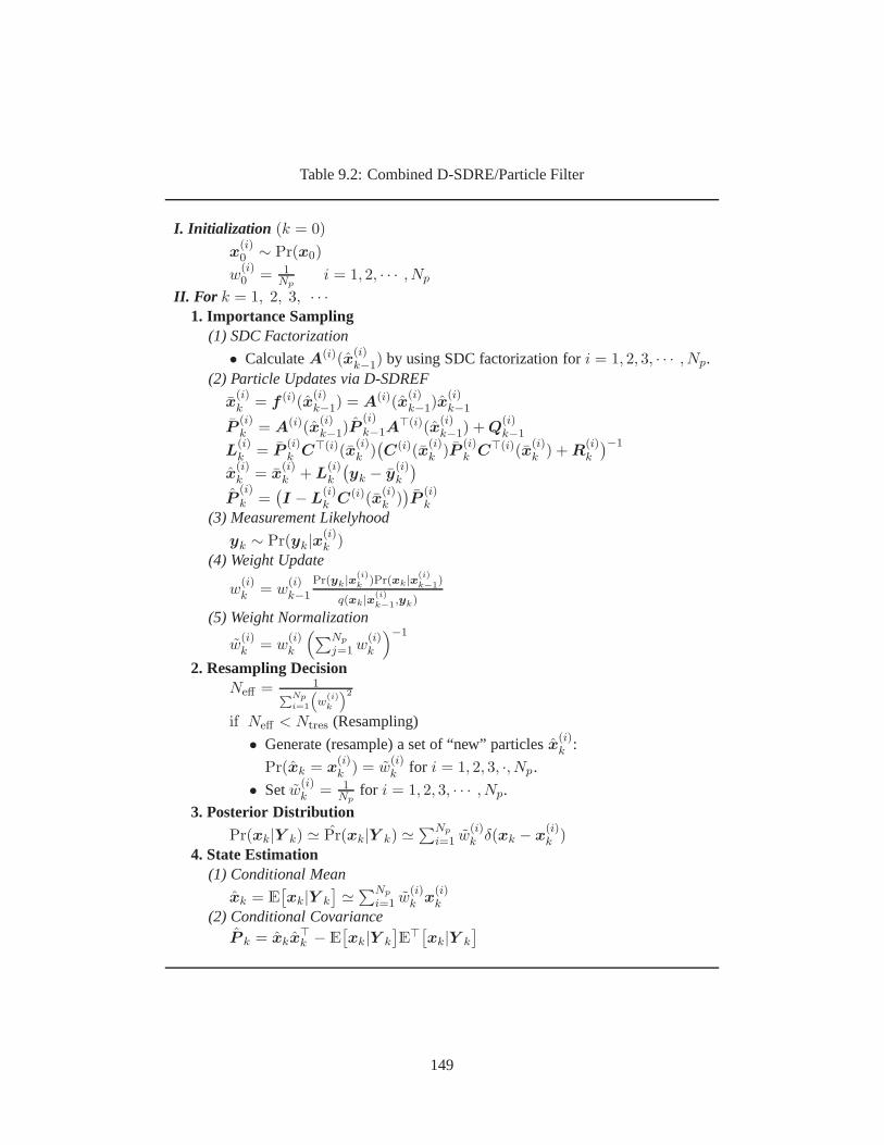
Table 9.2: Combined D-SDRE/Particle Filter
I. Initialization (k = 0)
x(i)0 ∼ Pr(x0)
w(i)0 = 1
Npi = 1, 2, · · · , Np
II. For k = 1, 2, 3, · · ·1. Importance Sampling
(1) SDC Factorization
• CalculateA(i)(x(i)k−1) by using SDC factorization fori = 1, 2, 3, · · · , Np.
(2) Particle Updates via D-SDREF
x(i)k = f (i)(x
(i)k−1) = A(i)(x
(i)k−1)x
(i)k−1
P(i)k = A(i)(x
(i)k−1)P
(i)k−1A
⊤(i)(x(i)k−1) +Q
(i)k−1
L(i)k = P
(i)k C⊤(i)(x
(i)k )(C(i)(x
(i)k )P
(i)k C⊤(i)(x
(i)k ) +R
(i)k
)−1
x(i)k = x
(i)k +L
(i)k
(yk − y
(i)k
)
P(i)k =
(I −L
(i)k C(i)(x
(i)k ))P
(i)k
(3) Measurement Likelyhood
yk ∼ Pr(yk|x(i)k )
(4) Weight Update
w(i)k = w
(i)k−1
Pr(yk |x(i)k
)Pr(xk|x(i)k−1)
q(xk|x(i)k−1,yk)
(5) Weight Normalization
w(i)k = w
(i)k
(∑Np
j=1w(i)k
)−1
2. Resampling DecisionNeff = 1
∑Npi=1
(
w(i)k
)2
if Neff < Ntres (Resampling)
• Generate (resample) a set of “new” particlesx(i)k :
Pr(xk = x(i)k ) = w
(i)k for i = 1, 2, 3, ·, Np.
• Setw(i)k = 1
Npfor i = 1, 2, 3, · · · , Np.
3. Posterior Distribution
Pr(xk|Y k) ≃ Pr(xk|Y k) ≃∑Np
i=1 w(i)k δ(xk − x
(i)k )
4. State Estimation(1) Conditional Mean
xk = E[xk|Y k
]≃∑Np
i=1 w(i)k x
(i)k
(2) Conditional CovarianceP k = xkx
⊤k − E
[xk|Y k
]E
⊤[xk|Y k
]
149
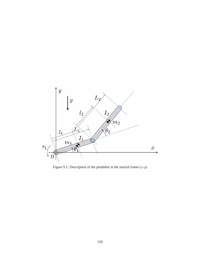
Figure 9.1: Description of the pendubot in the inertial frame (x-y)
150
whereℓi (i = 1, 2, · · · , 5) are parameters defined as
ℓ1 = m1l21 +m2L
21 + I1
ℓ2 = m2l22 + I2
ℓ3 = m2L1l2
ℓ4 = m1l1 +m2L1
ℓ5 = m2l2.
Assuming that there is no actuator in the system, i.e.,τ1 = 0, the state-space equation of the pendubot
system can be derived from (9.26):
q
q
︸︷︷︸
=:x
=
0 I2×2
−M−1g
[
q−11 ηq1 q−1
2 ηq2
]
−M−1
(
V + g
[
q−11 ηq1 q−1
2 ηq2
])
︸ ︷︷ ︸
=:A(x)
q
q
︸︷︷︸
=:x
(9.27)
whereI2×2 ∈ R2×2 is the identity matrix andηi (i = q1, q2, q1, q2) is an indicator function such that
ηi = 1 if |i| = max |q1|, |q2|, |q1|, |q2|
ηi = 0 otherwise.(9.28)
It is assumed that onlyq = [θ1 θ2]⊤ is measurable. Definingx =
xk+1−xk
T whereT is the sampling
time and addingGkωk (Gk := TQ12k , ωk ∼ N (04, I4)) as a process noise andΓνk (Γk := TR
12k , νk ∼
N (02, I2)) as a measurement noise yield the discrete-time state-space equation of (9.27):
xk+1 =(
I4×4 + TA(xk))
xk +Gkωk
yk =
[
I2×2 02×2
]
︸ ︷︷ ︸
Ck
xk + Γkνk. (9.29)
The physical parameters of the pendubot for simulation are as follows:m1 = m2 = 1 kg, I1 = 1 kgm2,
I2 = 0.6 kgm2, L1 = 1 m, L2 = 1.3 m, l1 = 0.5 m, andl2 = 0.6 m. The sampling time isT = 0.01 sec.
The initial conditions of the states are[θ1,0 θ2,0 θ1,0 θ2,0]⊤ = [π2
π12 0 0]⊤. Three different filters
are performed to evaluate the performance of the D-SDREF: EKF, UKF, and the D-SDREF. The initial
151
estimates of the states for the filters are set to[θ1,0 θ2,0ˆθ1,0
ˆθ2,0]
⊤ = [π3 − π6 0 0]⊤.
Two cases are simulated with differentQk andRk. For the first simulation, we set upQk andRk as
Qk = diag([0.001, 0.001, 0.001, 0.001]) andRk = diag([0.1, 0.1]), which defines smaller Gaussian
noises in the pendubot system. Figure 9.2 shows the simulation results of the state trajectories and root-
mean square (RMS) errors by the EKF, UKF, and D-SDREF. When such small noises were applied, the
performance of the D-SDREF is similar to that by the UKF whilethe EKF failed, especially to estimate
accurate rates of angles (ˆθ1 and ˆθ2 in Figure 9.2(a)). It shows that the linearization of the dynamical system
can affect the performance of the filters, which is one of the main drawbacks of using EKF in a highly
nonlinear system.
Increasing the values ofQk andRk, the reliability of the proposed D-SDREF can be evaluated. Figure 9.3
shows the simulation results of the filters withQk = diag([0.1, 0.1, 0.1, 0.1]) andRk = diag([1.0, 1.0])
which show relatively larger Gaussian noises in the pendubot system. It is interesting to note that EKF and
UKF failed to obtain accurate state estimates while the proposed D-SDREF shows the estimated the angles
and the rates of angles with smaller errors regardless ofQk andRk.
In the next part, we evaluate the combined D-SDRE/PF for a nonlinear system in the presence non-
Gaussian noises.
9.5.2 Motion Estimates of the Rössler Attractor with Non-Gaussian Noises
In this section, the proposed D-SDREF and the combined D-SDRE/PF are evaluated. To this end, we
use Rössler attractor (Rössler, 1976; Pikovsky et al., 1996), which shows chaotic behaviors with different
fractal properties of the attractor. The equations of the Rössler attractor have the following set of ordinary
differential equations:
x = −y − z
y = x+ ay
z = b+ z(x− c)
(9.30)
wherea, b, andc are design parameters. Figure 9.4 shows the trajectories ofx, y, andz of the Rössler
attractor in the 3-dimensional space witha = 0.2, b = 0.2, andc = 5.7.
152
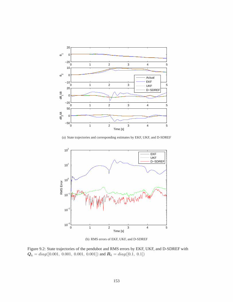
0 1 2 3 4 5−20
0
20
θ 1
0 1 2 3 4 5−10
0
10
θ 2
0 1 2 3 4 5−20
0
20
dθ1/d
t
0 1 2 3 4 5−50
0
50
dθ2/d
t
Time [s]
ActualEKFUKFD−SDREF
(a) State trajectories and corresponding estimates by EKF,UKF, and D-SDREF
0 1 2 3 4 510
−3
10−2
10−1
100
101
102
Time [s]
RM
S E
rror
EKFUKFD−SDREF
(b) RMS errors of EKF, UKF, and D-SDREF
Figure 9.2: State trajectories of the pendubot and RMS errors by EKF, UKF, and D-SDREF withQk = diag([0.001, 0.001, 0.001, 0.001]) andRk = diag([0.1, 0.1])
153

0 1 2 3 4 5−20
0
20
θ 1
0 1 2 3 4 5−20
0
20
θ 2
0 1 2 3 4 5−50
0
50
dθ1/d
t
0 1 2 3 4 5−100
0
100
dθ2/d
t
Time [s]
ActualEKFUKFD−SDREF
(a) State trajectories and corresponding estimates by EKF,UKF, and D-SDREF
0 1 2 3 4 510
−2
10−1
100
101
102
Time [s]
RM
S E
rror
EKFUKFD−SDREF
(b) RMS errors of EKF, UKF, and D-SDREF
Figure 9.3: State trajectories of the pendubot and RMS errors by EKF, UKF, and D-SDREF withQk = diag([0.1, 0.1, 0.1, 0.1]) andRk = diag([1.0, 1.0])
154
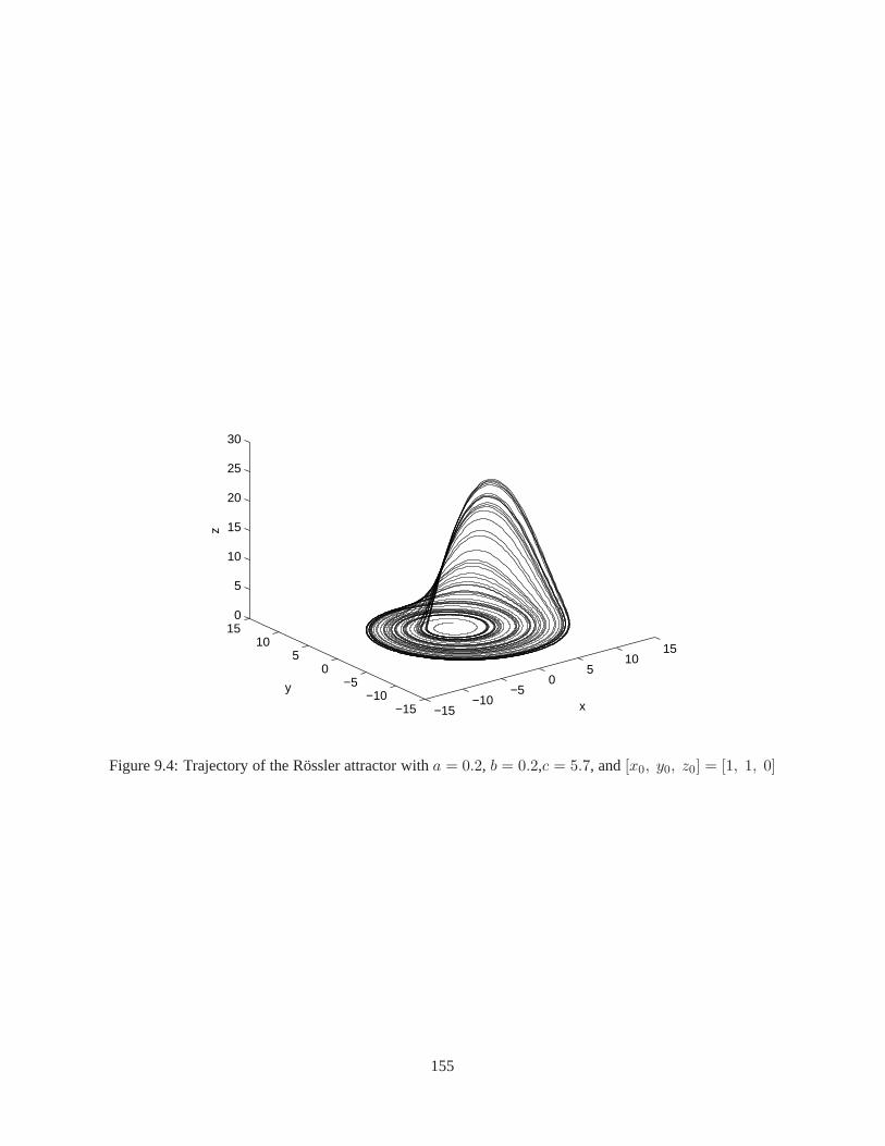
−15−10
−50
510
15
−15−10
−50
510
150
5
10
15
20
25
30
x
y
z
Figure 9.4: Trajectory of the Rössler attractor witha = 0.2, b = 0.2,c = 5.7, and[x0, y0, z0] = [1, 1, 0]
155
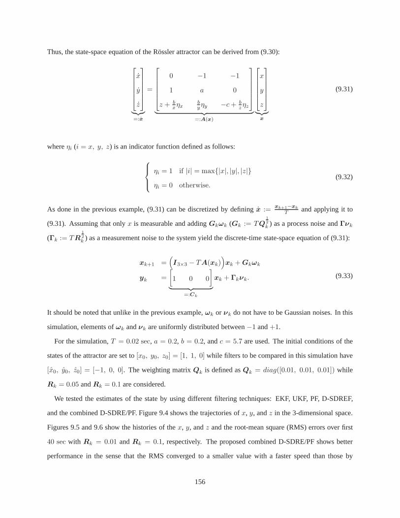
Thus, the state-space equation of the Rössler attractor canbe derived from (9.30):
x
y
z
︸︷︷︸
=:x
=
0 −1 −1
1 a 0
z + bxηx
byηy −c+ b
zηz
︸ ︷︷ ︸
=:A(x)
x
y
z
︸︷︷︸
x
(9.31)
whereηi (i = x, y, z) is an indicator function defined as follows:
ηi = 1 if |i| = max|x|, |y|, |z|
ηi = 0 otherwise.(9.32)
As done in the previous example, (9.31) can be discretized bydefining x :=xk+1−xk
T and applying it to
(9.31). Assuming that onlyx is measurable and addingGkωk (Gk := TQ12k ) as a process noise andΓνk
(Γk := TR12k ) as a measurement noise to the system yield the discrete-time state-space equation of (9.31):
xk+1 =(
I3×3 − TA(xk))
xk +Gkωk
yk =
[
1 0 0
]
︸ ︷︷ ︸
=:Ck
xk + Γkνk. (9.33)
It should be noted that unlike in the previous example,ωk or νk do not have to be Gaussian noises. In this
simulation, elements ofωk andνk are uniformly distributed between−1 and+1.
For the simulation,T = 0.02 sec, a = 0.2, b = 0.2, andc = 5.7 are used. The initial conditions of the
states of the attractor are set to[x0, y0, z0] = [1, 1, 0] while filters to be compared in this simulation have
[x0, y0, z0] = [−1, 0, 0]. The weighting matrixQk is defined asQk = diag([0.01, 0.01, 0.01]) while
Rk = 0.05 andRk = 0.1 are considered.
We tested the estimates of the state by using different filtering techniques: EKF, UKF, PF, D-SDREF,
and the combined D-SDRE/PF. Figure 9.4 shows the trajectories ofx, y, andz in the 3-dimensional space.
Figures 9.5 and 9.6 show the histories of thex, y, andz and the root-mean square (RMS) errors over first
40 sec with Rk = 0.01 andRk = 0.1, respectively. The proposed combined D-SDRE/PF shows better
performance in the sense that the RMS converged to a smaller value with a faster speed than those by
156
other filters and remained the small value while UKF and PF were more sensitive toRk than other filters.
Although UKF showed relatively similar performance to D-SDREF and the combined D-SDRE/PF, the time
to converge to small RMS is longer than the D-SDREF and the combined D-SDRE/PF.
9.6 Concluding Remarks
In this chapter, we introduced D-SDREF and derived its analytical form with two-step procedure. The
error bounds by the D-SDREF were investigated and the difference between the measured signal and the
estimated signals was proven to be ISS. We further extended the D-SDREF to deal with non-Gaussian
distributed noises. We suggested algorithms of the D-SDREFand the combined D-SDRE/PF. Finally, the
proposed filtering techniques were evaluated by using two challenging dynamical examples and the results
showed how the proposed filtering techniques could estimatethe actual values of the states of the dynamical
systems more accurately.
157

0 10 20 30 40 50−20
0
20
x
0 10 20 30 40 50−20
0
20
y
0 10 20 30 40 50
0
20
40
z
Time [s]
ActualEKFUKFPFD−SDREFD−SDRE/PF
(a) State trajectory of the Rössler attractor and its corresponding estimates by filters
0 10 20 30 40 5010
−4
10−3
10−2
10−1
100
101
102
Time [s]
RM
S E
rror
EKFUKFPFD−SDREFD−SDRE/PF
(b) RMS errors of the estimates
Figure 9.5: State trajectory/estimates of the Rössler attractor and RMS errors by EKF, UKF, particle filter,D-SDREF, and combined D-SDRE/PF under uniform noises withQk = diag([0.01, 0.01, 0.01]), Rk = 0.01
158
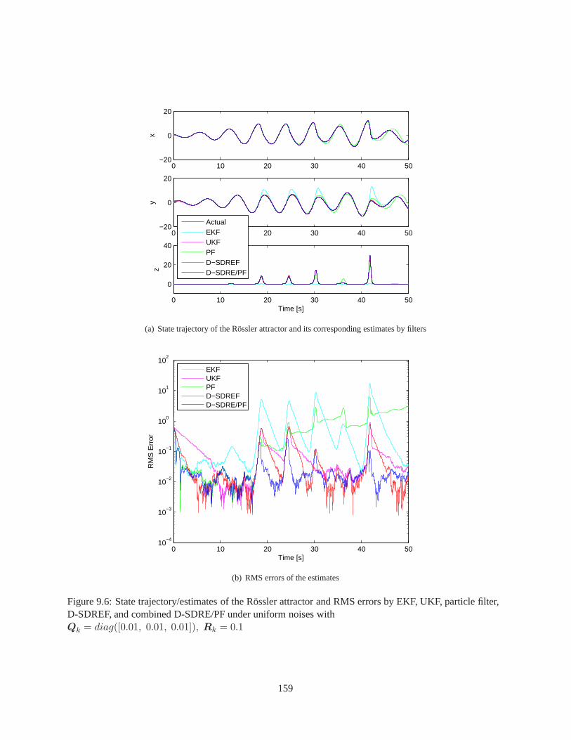
0 10 20 30 40 50−20
0
20
x
0 10 20 30 40 50−20
0
20
y
0 10 20 30 40 50
0
20
40
z
Time [s]
ActualEKFUKFPFD−SDREFD−SDRE/PF
(a) State trajectory of the Rössler attractor and its corresponding estimates by filters
0 10 20 30 40 5010
−4
10−3
10−2
10−1
100
101
102
Time [s]
RM
S E
rror
EKFUKFPFD−SDREFD−SDRE/PF
(b) RMS errors of the estimates
Figure 9.6: State trajectory/estimates of the Rössler attractor and RMS errors by EKF, UKF, particle filter,D-SDREF, and combined D-SDRE/PF under uniform noises withQk = diag([0.01, 0.01, 0.01]), Rk = 0.1
159

Part IV
Conclusions and Future Work
160
Chapter 10
Conclusions and Future Research
TO conclude, the main contributions of the thesis are summarized and some directions of future research
are presented next.
10.1 Summary
In this thesis, we have discussed control and estimation methodologies by using the D-SDRE and CD-SDRE
technique, specifically in the presence of constraints on the inputs or states.
In Part II, we investigated the design of the D-SDRE and CD-SDRE controllers. In Chapter 5, Detailed
procedures of deriving the D-SDRE and CD-SDRE were providedfor the deterministic nonlinear systems.
A concept of model predictive control was used not only to provide estimated values of the parameters
in the D-SDRE technique, but also to handle constraints on the states/inputs. The proofs of the stability
condition for the D-SDRE and the CD-SDRE feedback systems were analyzed to show the exponential
stability in their ROAs. In the subsequent chapter, the proposed CD-SDRE controller was evaluated by
using challenging problems in spacecraft orbit reconfiguration. We also derived high-fidelity models of the
reference and the relative orbit in the presence of the oblateness of the Earth (J2 perturbation). The proposed
CD-SDRE controller successfully generated control signals to transfer the orbit even with demanding initial
conditions and the stringent input saturations.
In Chapter 7, the robust CD-SDRE controller was studied for aclass of uncertain nonlinear systems. Two
controllers were used as in the CD-SDRE discussed in the previous chapter: the robust D-SDRE controller
and the robust MPC. The proposed robust CD-SDRE controller comprises the two controllers and they are
activated exclusively, which can be viewed as a switched system. We derived 3-dimensional equations of
motion of the spacecraft attitude in the presence of fuel slosh effect. Applications of the robust CD-SDRE
controller to stabilizing the attitude motion showed its reliability in the presence of uncertainties due to the
161

motion of the fuel while moving the spacecraft attitude and the saturations on its applied torques.
In Part III, we discussed the filtering design based on the D-SDRE technique. In Chapter 8, the D-SDRE
Observer was derived and the stability analysis of the errorbetween the actual states and their associated
signals estimated by the D-SDRE Observer was provided to be input-to-state stable.
In Chapter 9, two filters were proposed: the D-SDRE-based filter and the combined D-SDRE/particle
filter. The D-SDREF can be used for the nonlinear system with Gaussian noises while the combined D-
SDRE/PF for the system with non-Gaussian noises as well as Gaussian noises. The error bounds for the
D-SDREF were analyzed. Algorithms of the D-SDREF and the combined D-SDRE/PF were provided.
We also provided related studies to the CD-SDRE technique. In Chapter 3, exponential stability of the
continuous-time SDRE feedback system was investigated through the use of contraction analysis and the
incremental stability analysis. A way to estimate the ROA was provided which is guaranteed to be invariant.
In Chapter 4, a gain-tuning algorithm was discussed, calledthe AGT-PSO. It provides systematic way to
find optimal values of the tuning parameters such as controller gains, system parameters, etc. Due to the
model independence of the AGT-PSO and the characteristics of the non-gradient-based method, it is easily
applicable to various practical problems. We applied the AGT-PSO to industry applications and showed its
effectiveness.
10.2 Future Research
10.2.1 Output-Feedback Control via the CD-SDRE Technique
In this thesis, we discussed the CD-SDRE controller for the full-state feedback system. Moreover, we
designed an observer and the filters via the D-SDRE technique. Therefore, output-feedback control of the
CD-SDRE controller can be investigated by combining the twosystems. In this case, the stability of the
combined system will be a main issue.
10.2.2 Adaptive D-SDRE/CD-SDRE Controller
In Chapter 7, we discussed uncertainties in a nonlinear model to be controlled by the CD-SDRE technique.
The model uncertainties can be estimated or the effect of themodel mismatches can be compensated by
using a concept of adaptive control (Narendra and Annaswamy, 1989; Krstic et al., 1995; Ioannou and Sun,
162

1995). Therefore, it is worthwhile to investigate the adaptive version of the D-SDRE/CD-SDRE technique.
10.2.3 SDRE-BasedH∞ Control
The SDRE (or D-SDRE) can be applied to design a robust controller viaH∞ control (Doyle et al., 1991;
Zhou et al., 1996). As discussed briefly in (Cloutier, 1997),the SDRE technique can be extended to non-
linearH∞ control due to its analogy to linear quadratic regulation orlinear quadratic Gaussian controllers.
However, more rigorous analysis of the stability conditionshould be investigated in case of a finite horizon
problem. Unlike the infinite horizon problem, which makes the control problem similar to LQR and LQG
controllers, the generalized continuous-time (or discrete-time) Riccati equation as discussed in Chapter 5
should be used if a finite horizon is considered.
163
References
Agrawal, B. N., July–August 1993. Dynamic Characteristicsof Liquid Motion in Partially Filled Tanks of aSpinning Spacecraft. AIAA Journal of Guidance, Control, and Dynamics 16 (4), 636–640.
Alfriend, K. T., Vadali, S. R., Gurfil, P., How, J. P., Breger,L. S., 2010. Spacecraft Formation Flying:Dynamics, Control and Navigation. Elsevier, Oxford, England.
Anderson, B. D. O., Moore, J. B., 1979. Optimal Filtering. Prentice-Hall, Inc., Englewood Cliffs, NJ,reprinted by Dover, Mineola, NY, 2005.
Anderson, R. T., May 2010. Results and Control Law Derivations for Hystat Pressure Control (HPC), HystatTorque Control (HTC), and Variable ePOR Features. Tech. Rep. 23-03233, Caterpillar Inc., Mossville,IL.
Angeli, D., March 2002. A Lyapunov Approach to Incremental Stability Properties. IEEE Transactions onAutomatic Control 47 (3), 410–421.
Åström, K. J., Hägglund, T., Hang, C. C., Ho, W. K., August 1993. Automatic Tuning and Adaptation forPID Controllers — A Survey. Control Engineering Practice 1 (4), 699–714.
Banks, H. T., Kwon, H.-D., Toivanen, J. A., Tran, H. T., March–April 2006. A State-Dependent RiccatiEquation-Based Estimator Approach for HIV Feedback Control. Optimal Control Applications and Meth-ods 27 (2), 93–121.
Batmani, Y., Khaloozadeh, H., September/October 2012. Optimal Chemotheraph in Cancer Treatment:State Dependent Riccati Equation Control and Extended Kalman Filter. Optimal Control Applicationsand Methods 34 (5), 562–577.
Beikzadeh, H., Taghirad, H. D., August 2012a. Exponential Nonlinear Observer Based on the DifferentialState-Dependent Riccati Equation. International Journalof Automation and Computing 9 (4), 358–368.
Beikzadeh, H., Taghirad, H. D., January 2012b. Robust SDRE Filter Design for Nonlinear Uncertain Sys-tems with anH∞ Performance Criterion. ISA Transactions 51 (1), 146–152.
Bemporad, A., Morari, M., Dua, V., Pistikopoulos, E. N., January 2002. The Explicit Linear QuadraticRegulator for Constrained Systems. Automatica 38 (1), 3–20.
Bentsman, J., Chang, I., Li, W., August 2012. Demonstrationof Automatic Gain-Tuners via Iterative Feed-back Tuning and Particle Swarm Optimization: Feasibility Study. Tech. rep., Caterpillar Inc., Mossville,IL, CAT-1065512.
Bogdanov, A., Wan, E., January–February 2007. State-Dependent Riccati Equation Control for Small Au-tonomous Helicopters. AIAA Journal of Guidance, Control, and Dynamics 30 (1), 47–60.
164
Boyd, S., Ghaoui, L. E., Feron, E., Balakrishnan, V., 1994. Linear Matrix Inequalities in System and ControlTheory. SIAM, Philadelphia, PA.
Bracci, A., Innocenti, M., Pollini, L., November–December2006. Estimation of the Region of Attractionfor State-Dependent Riccati Equation Controllers. AIAA Journal of Guidance, Control, and Dynamics29 (6), 1427–1430.
Brown, R. G., Hwang, P. Y. C., 1997. Introduction to Random Signals and Applied Kalman Filtering, 3rdEdition. John Wiley & Sons, New York, NY.
Bryson, Jr., A. E., 1994. Control of Spacecraft and Aircraft. Princeton University Press, Princeton, NJ.
Bryson, Jr., A. E., Ho, Y.-C., 1975. Applied Optimal Control: Optimization, Estimation, and Control. Taylor& Francis, New York, NY.
Campi, M. C., Lecchini, A., Savaresi, S. M., August 2002. Virtual Reference Feedback Tuning: A directMethod for the Design of Feedback Controllers. Automatica 38 (8), 1337–1346.
Campi, M. C., Savaresi, S. M., January 2006. Direct Nonlinear Control Design: The Virtual ReferenceFeedback Tuning (VRFT) Approach. IEEE Transactions on Automatic Control 51 (1), 14–27.
Chang, I., Chung, S.-J., Blackmore, L., December 2010a. Cooperative Control with Adaptive Graph Lapla-cians for Spacecraft Formation Flying. In: 49th IEEE Conference on Decision and Control. Atlanta, GA,pp. 4926–4933.
Chang, I., Chung, S.-J., Hadaegh, F. Y., May 2011. Novel Coordinate Transformation and Robust Co-operative Formation Control for Swarms of Spacecraft. In: 4th International Conference on SpacecraftFormation Flying Missions & Technologies. St. Hubert, Québec, Canada.
Chang, I., Li, W., Bentsman, J., February 2013. Developmentand Performance Evaluation of AutomaticGain-Tuner. Tech. rep., Caterpillar Inc., Mossville, IL, CAT-1067515.
Chang, I., Park, S.-Y., Choi, K.-H., October 2009. Decentralized Coordinated Attitude Control for SatelliteFormation Flying via the State-Dependent Riccati EquationTechnique. International Journal of Non-Linear Mechanics 44 (8), 891–904.
Chang, I., Park, S.-Y., Choi, K.-H., October 2010b. Nonlinear Attitude Control of a Tether-Connected Multi-Satellite in Three-Dimensional Space. IEEE Transactions on Aerospace and Electronic Systems 46 (4),1950–1968.
Chen, C.-C., Liang, Y.-W., Jhu, W.-M., October 2015. GlobalStability of a System with State-DependentRiccati Equation Controller. AIAA Journal of Guidance, Control, and Dynamics 38 (10), 2050–2054.
Çimen, T., June 2008. State-Dependent Riccati Equation (SDRE) Control: A Survey. In: 17th IFAC WorldCongress. Seoul, Korea, pp. 3761–3775.
Çimen, T., April 2010. Systematic and Effective Design of Nonlinear Feedback Controllers via the State-Dependent Riccati Equation (SDRE) Method. Annual Reviews in Control 34 (1), 32–51.
Çimen, T., July–August 2012. Survey of State-Dependent Riccati Equation in Nonlinear Optimal FeedbackControl Synthesis. AIAA Journal of Guidance, Control, and Dynamics 35 (4), 1025–1047.
165
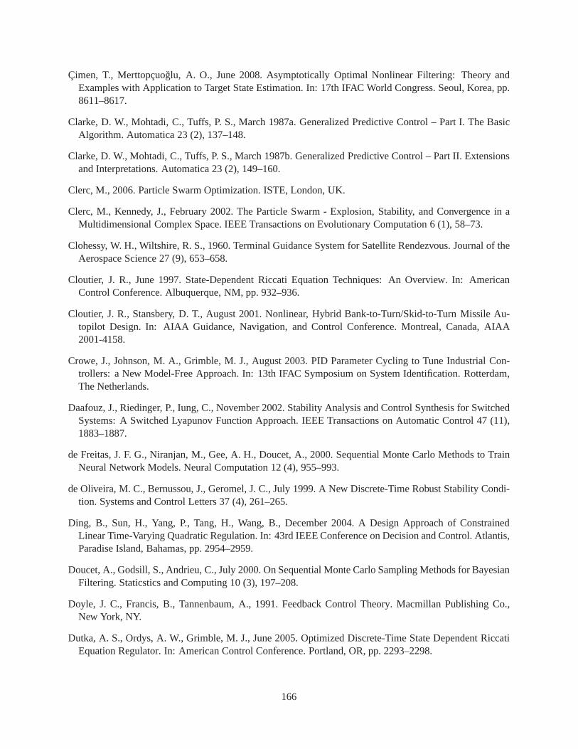
Çimen, T., Merttopçuoglu, A. O., June 2008. Asymptotically Optimal Nonlinear Filtering: Theory andExamples with Application to Target State Estimation. In: 17th IFAC World Congress. Seoul, Korea, pp.8611–8617.
Clarke, D. W., Mohtadi, C., Tuffs, P. S., March 1987a. Generalized Predictive Control – Part I. The BasicAlgorithm. Automatica 23 (2), 137–148.
Clarke, D. W., Mohtadi, C., Tuffs, P. S., March 1987b. Generalized Predictive Control – Part II. Extensionsand Interpretations. Automatica 23 (2), 149–160.
Clerc, M., 2006. Particle Swarm Optimization. ISTE, London, UK.
Clerc, M., Kennedy, J., February 2002. The Particle Swarm - Explosion, Stability, and Convergence in aMultidimensional Complex Space. IEEE Transactions on Evolutionary Computation 6 (1), 58–73.
Clohessy, W. H., Wiltshire, R. S., 1960. Terminal Guidance System for Satellite Rendezvous. Journal of theAerospace Science 27 (9), 653–658.
Cloutier, J. R., June 1997. State-Dependent Riccati Equation Techniques: An Overview. In: AmericanControl Conference. Albuquerque, NM, pp. 932–936.
Cloutier, J. R., Stansbery, D. T., August 2001. Nonlinear, Hybrid Bank-to-Turn/Skid-to-Turn Missile Au-topilot Design. In: AIAA Guidance, Navigation, and ControlConference. Montreal, Canada, AIAA2001-4158.
Crowe, J., Johnson, M. A., Grimble, M. J., August 2003. PID Parameter Cycling to Tune Industrial Con-trollers: a New Model-Free Approach. In: 13th IFAC Symposium on System Identification. Rotterdam,The Netherlands.
Daafouz, J., Riedinger, P., Iung, C., November 2002. Stability Analysis and Control Synthesis for SwitchedSystems: A Switched Lyapunov Function Approach. IEEE Transactions on Automatic Control 47 (11),1883–1887.
de Freitas, J. F. G., Niranjan, M., Gee, A. H., Doucet, A., 2000. Sequential Monte Carlo Methods to TrainNeural Network Models. Neural Computation 12 (4), 955–993.
de Oliveira, M. C., Bernussou, J., Geromel, J. C., July 1999.A New Discrete-Time Robust Stability Condi-tion. Systems and Control Letters 37 (4), 261–265.
Ding, B., Sun, H., Yang, P., Tang, H., Wang, B., December 2004. A Design Approach of ConstrainedLinear Time-Varying Quadratic Regulation. In: 43rd IEEE Conference on Decision and Control. Atlantis,Paradise Island, Bahamas, pp. 2954–2959.
Doucet, A., Godsill, S., Andrieu, C., July 2000. On Sequential Monte Carlo Sampling Methods for BayesianFiltering. Staticstics and Computing 10 (3), 197–208.
Doyle, J. C., Francis, B., Tannenbaum, A., 1991. Feedback Control Theory. Macmillan Publishing Co.,New York, NY.
Dutka, A. S., Ordys, A. W., Grimble, M. J., June 2005. Optimized Discrete-Time State Dependent RiccatiEquation Regulator. In: American Control Conference. Portland, OR, pp. 2293–2298.
166
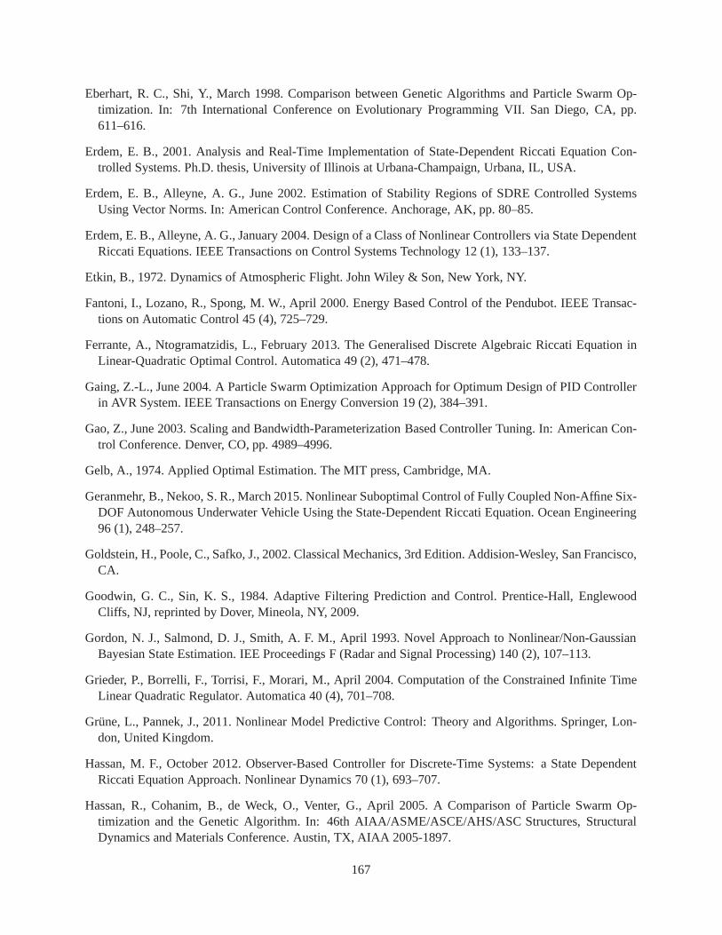
Eberhart, R. C., Shi, Y., March 1998. Comparison between Genetic Algorithms and Particle Swarm Op-timization. In: 7th International Conference on Evolutionary Programming VII. San Diego, CA, pp.611–616.
Erdem, E. B., 2001. Analysis and Real-Time Implementation of State-Dependent Riccati Equation Con-trolled Systems. Ph.D. thesis, University of Illinois at Urbana-Champaign, Urbana, IL, USA.
Erdem, E. B., Alleyne, A. G., June 2002. Estimation of Stability Regions of SDRE Controlled SystemsUsing Vector Norms. In: American Control Conference. Anchorage, AK, pp. 80–85.
Erdem, E. B., Alleyne, A. G., January 2004. Design of a Class of Nonlinear Controllers via State DependentRiccati Equations. IEEE Transactions on Control Systems Technology 12 (1), 133–137.
Etkin, B., 1972. Dynamics of Atmospheric Flight. John Wiley& Son, New York, NY.
Fantoni, I., Lozano, R., Spong, M. W., April 2000. Energy Based Control of the Pendubot. IEEE Transac-tions on Automatic Control 45 (4), 725–729.
Ferrante, A., Ntogramatzidis, L., February 2013. The Generalised Discrete Algebraic Riccati Equation inLinear-Quadratic Optimal Control. Automatica 49 (2), 471–478.
Gaing, Z.-L., June 2004. A Particle Swarm Optimization Approach for Optimum Design of PID Controllerin AVR System. IEEE Transactions on Energy Conversion 19 (2), 384–391.
Gao, Z., June 2003. Scaling and Bandwidth-Parameterization Based Controller Tuning. In: American Con-trol Conference. Denver, CO, pp. 4989–4996.
Gelb, A., 1974. Applied Optimal Estimation. The MIT press, Cambridge, MA.
Geranmehr, B., Nekoo, S. R., March 2015. Nonlinear Suboptimal Control of Fully Coupled Non-Affine Six-DOF Autonomous Underwater Vehicle Using the State-Dependent Riccati Equation. Ocean Engineering96 (1), 248–257.
Goldstein, H., Poole, C., Safko, J., 2002. Classical Mechanics, 3rd Edition. Addision-Wesley, San Francisco,CA.
Goodwin, G. C., Sin, K. S., 1984. Adaptive Filtering Prediction and Control. Prentice-Hall, EnglewoodCliffs, NJ, reprinted by Dover, Mineola, NY, 2009.
Gordon, N. J., Salmond, D. J., Smith, A. F. M., April 1993. Novel Approach to Nonlinear/Non-GaussianBayesian State Estimation. IEE Proceedings F (Radar and Signal Processing) 140 (2), 107–113.
Grieder, P., Borrelli, F., Torrisi, F., Morari, M., April 2004. Computation of the Constrained Infinite TimeLinear Quadratic Regulator. Automatica 40 (4), 701–708.
Grüne, L., Pannek, J., 2011. Nonlinear Model Predictive Control: Theory and Algorithms. Springer, Lon-don, United Kingdom.
Hassan, M. F., October 2012. Observer-Based Controller forDiscrete-Time Systems: a State DependentRiccati Equation Approach. Nonlinear Dynamics 70 (1), 693–707.
Hassan, R., Cohanim, B., de Weck, O., Venter, G., April 2005.A Comparison of Particle Swarm Op-timization and the Genetic Algorithm. In: 46th AIAA/ASME/ASCE/AHS/ASC Structures, StructuralDynamics and Materials Conference. Austin, TX, AIAA 2005-1897.
167
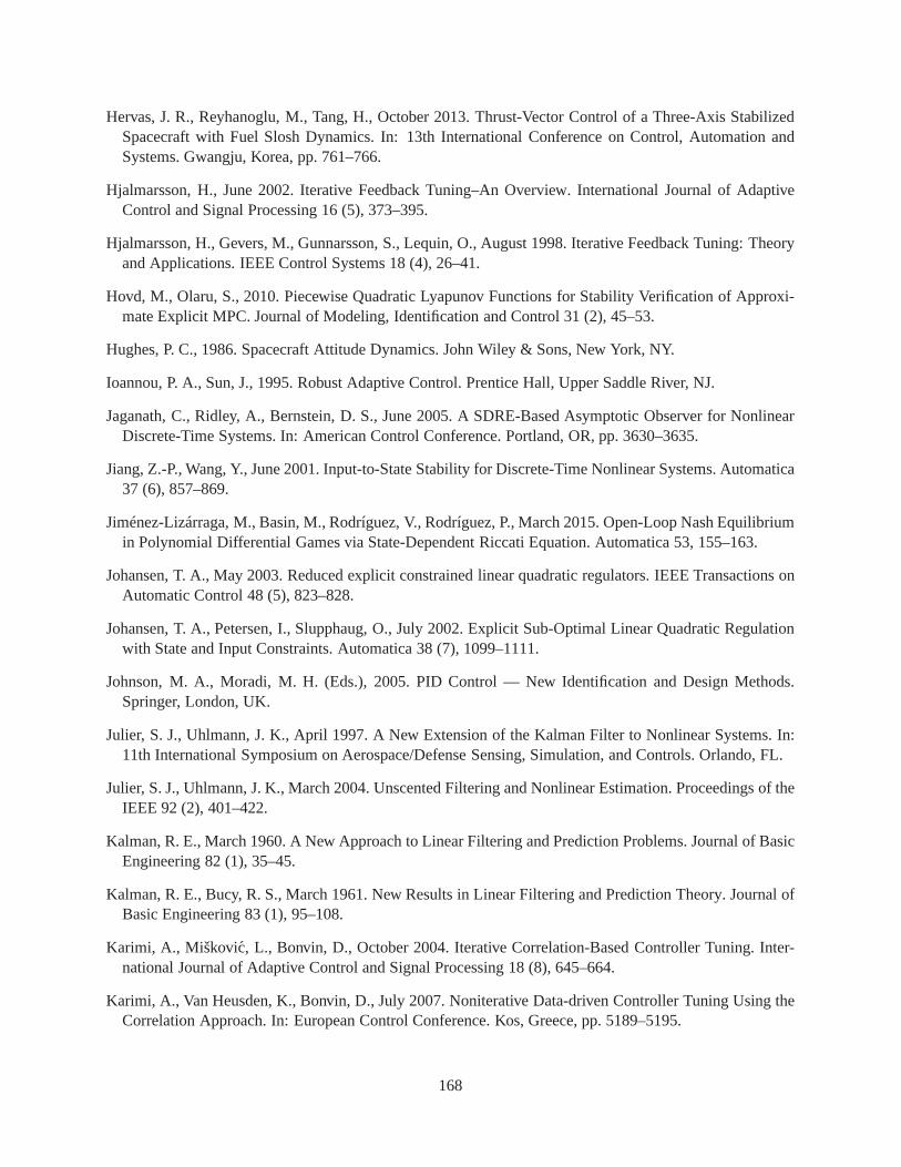
Hervas, J. R., Reyhanoglu, M., Tang, H., October 2013. Thrust-Vector Control of a Three-Axis StabilizedSpacecraft with Fuel Slosh Dynamics. In: 13th International Conference on Control, Automation andSystems. Gwangju, Korea, pp. 761–766.
Hjalmarsson, H., June 2002. Iterative Feedback Tuning–An Overview. International Journal of AdaptiveControl and Signal Processing 16 (5), 373–395.
Hjalmarsson, H., Gevers, M., Gunnarsson, S., Lequin, O., August 1998. Iterative Feedback Tuning: Theoryand Applications. IEEE Control Systems 18 (4), 26–41.
Hovd, M., Olaru, S., 2010. Piecewise Quadratic Lyapunov Functions for Stability Verification of Approxi-mate Explicit MPC. Journal of Modeling, Identification and Control 31 (2), 45–53.
Hughes, P. C., 1986. Spacecraft Attitude Dynamics. John Wiley & Sons, New York, NY.
Ioannou, P. A., Sun, J., 1995. Robust Adaptive Control. Prentice Hall, Upper Saddle River, NJ.
Jaganath, C., Ridley, A., Bernstein, D. S., June 2005. A SDRE-Based Asymptotic Observer for NonlinearDiscrete-Time Systems. In: American Control Conference. Portland, OR, pp. 3630–3635.
Jiang, Z.-P., Wang, Y., June 2001. Input-to-State Stability for Discrete-Time Nonlinear Systems. Automatica37 (6), 857–869.
Jiménez-Lizárraga, M., Basin, M., Rodríguez, V., Rodríguez, P., March 2015. Open-Loop Nash Equilibriumin Polynomial Differential Games via State-Dependent Riccati Equation. Automatica 53, 155–163.
Johansen, T. A., May 2003. Reduced explicit constrained linear quadratic regulators. IEEE Transactions onAutomatic Control 48 (5), 823–828.
Johansen, T. A., Petersen, I., Slupphaug, O., July 2002. Explicit Sub-Optimal Linear Quadratic Regulationwith State and Input Constraints. Automatica 38 (7), 1099–1111.
Johnson, M. A., Moradi, M. H. (Eds.), 2005. PID Control — New Identification and Design Methods.Springer, London, UK.
Julier, S. J., Uhlmann, J. K., April 1997. A New Extension of the Kalman Filter to Nonlinear Systems. In:11th International Symposium on Aerospace/Defense Sensing, Simulation, and Controls. Orlando, FL.
Julier, S. J., Uhlmann, J. K., March 2004. Unscented Filtering and Nonlinear Estimation. Proceedings of theIEEE 92 (2), 401–422.
Kalman, R. E., March 1960. A New Approach to Linear Filteringand Prediction Problems. Journal of BasicEngineering 82 (1), 35–45.
Kalman, R. E., Bucy, R. S., March 1961. New Results in Linear Filtering and Prediction Theory. Journal ofBasic Engineering 83 (1), 95–108.
Karimi, A., Miškovic, L., Bonvin, D., October 2004. Iterative Correlation-Based Controller Tuning. Inter-national Journal of Adaptive Control and Signal Processing18 (8), 645–664.
Karimi, A., Van Heusden, K., Bonvin, D., July 2007. Noniterative Data-driven Controller Tuning Using theCorrelation Approach. In: European Control Conference. Kos, Greece, pp. 5189–5195.
168

Kechichian, J. A., January–March 1998. Motion in General Elliptic Orbit with Respect to a Dragging andPrecessing Coordinate Frame. Journal of the AstronauticalSciences 46 (1), 25–45.
Kennedy, J., Eberhart, R., November 1995. Particle Swarm Optimization. In: IEEE International Conferenceon Neural Networks. Washington, DC, pp. 1942–1948.
Khalil, H. K., 2002. Nonlinear Systems, 3rd Edition. Prentice Hall, Upper Saddle River, NJ.
Kim, K., Rao, P., Burnworth, J. A., July-August 2010. Self-Tuning of the PID Controller for a DigitalExcitation Control System. IEEE Transactions on Industrial Applications 46 (4), 1518–1524.
Kim, T.-H., Maruta, I., Sugie, T., April 2008. Robust PID Controller Tuning Based on the ConstrainedParticle Swarm Optimization. Automatica 44 (4), 1104–1110.
Kirk, D. E., 1970. Optimal Control Theory: An Introduction.Prentice Hall, Englewood Cliffs, NJ, reprintedby Dover, Mineola, NY, 2004.
Kothare, M. V., Campo, P. J., Morari, M., Nett, C. N., December 1994. Unified Framework for the Study ofAnti-windup Designs. Automatica 30 (12), 1869–1883.
Kothare, M. V., Morari, M., May 1999. Multiplier Theory for Stability Analysis of Anti-Windup ControlSystems. Automatica 35 (5), 917–928.
Krstic, M., Kanellakopoulos, I., Kokotovic, P., 1995. Nonlinear and Adaptive Control Design. John Wiley& Sons, New York, NY.
Langson, W., Alleyne, A. G., September 2002. A Stability Result with Application to Nonlinear Regulation.Journal of Dynamic Systems, Measurement, and Control 124 (3), 452–456.
Lee, J.-W., Khargonekar, P. P., October 2007. Constrained Infinite-Horizon Linear Quadratic Regulation ofDiscrete-Time Systems. IEEE Transactions on Automatic Control 52 (10), 1951–1958.
Lequin, O., Gevers, M., Mossberg, M., Bosmans, E., Triest, L., September 2003. Iterative Feedback Tuningof PID Parameters: Comparison with Classical Tuning Rules.Control Engineering Practice 11 (9), 1023–1033.
Lewis, F. R., Vrabie, D. L., Syrmos, V. L., 2012. Optimal Control, 3rd Edition. John Wiley & Sons, Inc.,Hoboken, NJ.
Lohmiller, W., Slotine, J.-J. E., June 1998. On ContractionAnalysis for Non-Linear Systems. Automatica34 (6), 683–696.
Lorenz, E. N., March 1963. Deterministic Nonperiodic Flow.Journal of the Atmospheric Sciences 20 (2),130–141.
Luenberger, D. G., April 1966. Observers for MultivariableSystems. IEEE Transactions on AutomaticControl 11 (2), 190–197.
Magni, L., Raimondo, D. M., Allgöwer, F., 2009. Nonlinear Model Predictive Control: Towards New Chal-lenging Applications. Springer, Berlin Heidelberg.
Mayne, D. Q., Rawlings, J. B., Rao, C. V., Scokaert, P. O. M., June 2000. Constrained Model PredictiveControl: Stability and Optimality. Automatica 36 (6), 789–814.
169

McCaffrey, D., Banks, S. P., July 2001. Lagrangian Manifolds and Asymptotically Optimal StabilizingFeedback Control. Systems and Control Letters 43 (3), 219–224.
Mracek, C. P., Cloutier, J. R., April 1998. Control Designs for the Nonlinear Benchmark Problem via theState-Dependent Riccati Equation Method. International Journal of Robust and Nonlinear Control 8 (4–5), 401–433.
Naik, M. S., Singh, S. N., August 2007. State-Dependent Riccati Equation-Based Robust Dive Plane Controlof AUV with Control Constraints. Ocean Engineering 34 (11–12), 1711–1723.
Narendra, K. S., Annaswamy, A. M., 1989. Stable Adaptive Systems. Prentice Hall, Englewood Cliffs, NJ,reprinted by Dover, Mineola, NY, 2005.
Nazari, M., Ghaffari, A., Arab, F., 2015. Finite Duration Treatment of Cancer by Using Vaccine Therapy andOptimal Chemotherapy: State-Dependent Riccati Equation Control and Extended Kalman Filter. Journalof Biological Systems 23 (1), 1–29.
Nemra, A., Aouf, N., April 2010. Robust INS/GPS Sensor Fusion for UAV Localization Using SDRENonlinear Filtering. IEEE Sensors Journal 10 (4), 789–798.
Niknam, T., January 2010. A New Fuzzy Adaptive Hybrid Particle Swarm Optimization Algorithm for Non-Linear, Non-Smooth and Non-Convex Economic Dispatch Problem. Applied Energy 87 (1), 327–339.
Park, J.-B., Lee, K.-S., Shin, J.-R., Lee, K. Y., February 2005. A Particle Swarm Optimization for EconomicDispatch With Nonsmooth Cost Functions. IEEE Transactionson Power Systems 20 (1), 34–42.
Parrilo, P. A., May 2000. Structured Semi Definite Programs and Semi Algebraic Geometry Methods inRobustness and Optimization. Ph.D. thesis, California Institutte of Technology, Pasadena, CA, USA.
Parsopoulos, K. E., Vrahatis, M. N., 2002. Intelligent Technologies–Theory and Application: New Trendsin Intelligent Technologies. Vol. 76. IOS Press, Amsterdam, The Netherlands, Ch. Particle swarm opti-mization method for constrained optimization problems, pp. 214–220.
Parsopoulos, K. E., Vrahatis, M. N., 2010. Particle Swarm Optimization and Intelligence: Advances andApplications. IGI Global, Hershey, PA.
Pearson, J. D., 1962. Approximation Methods in Optimal Control I. Suboptimal Control. Journal of Elec-tronics and Control 13 (5), 453–469.
Peterson, L. D., Crawley, E. F., Hansman, R. J., September 1989. Nonlinear Fluid Slosh Coupled to theDynamics of Spacecraft. AIAA Journal 27 (9), 1230–1240.
Pham, Q. C., Tabareau, N., Slotine, J.-J. E., April 2009. A Contraction Theory Approach to StochasticIncremental Stability. IEEE Transactions on Automatic Control 54 (4), 816–820.
Pikovsky, A. S., Rosenblum, M. G., Kurths, J., 1996. Synchronization in a Population of Globally CoupledChaotic Oscillators. Europhysics Letters 34 (3), 165–170.
Poli, R., Kennedy, J., Blackwell, T., June 2007. Particle Swarm Optimization: An Overview. Swarm Intel-ligence 1 (1), 33–57.
Ramos, D. C. W., Peres, P. L. D., August 2001. A Less Conservative LMI Condition for the Robust Stabilityof Discrete-Time Uncertain Systems. Systems and Control Letters 43 (5), 371–378.
170
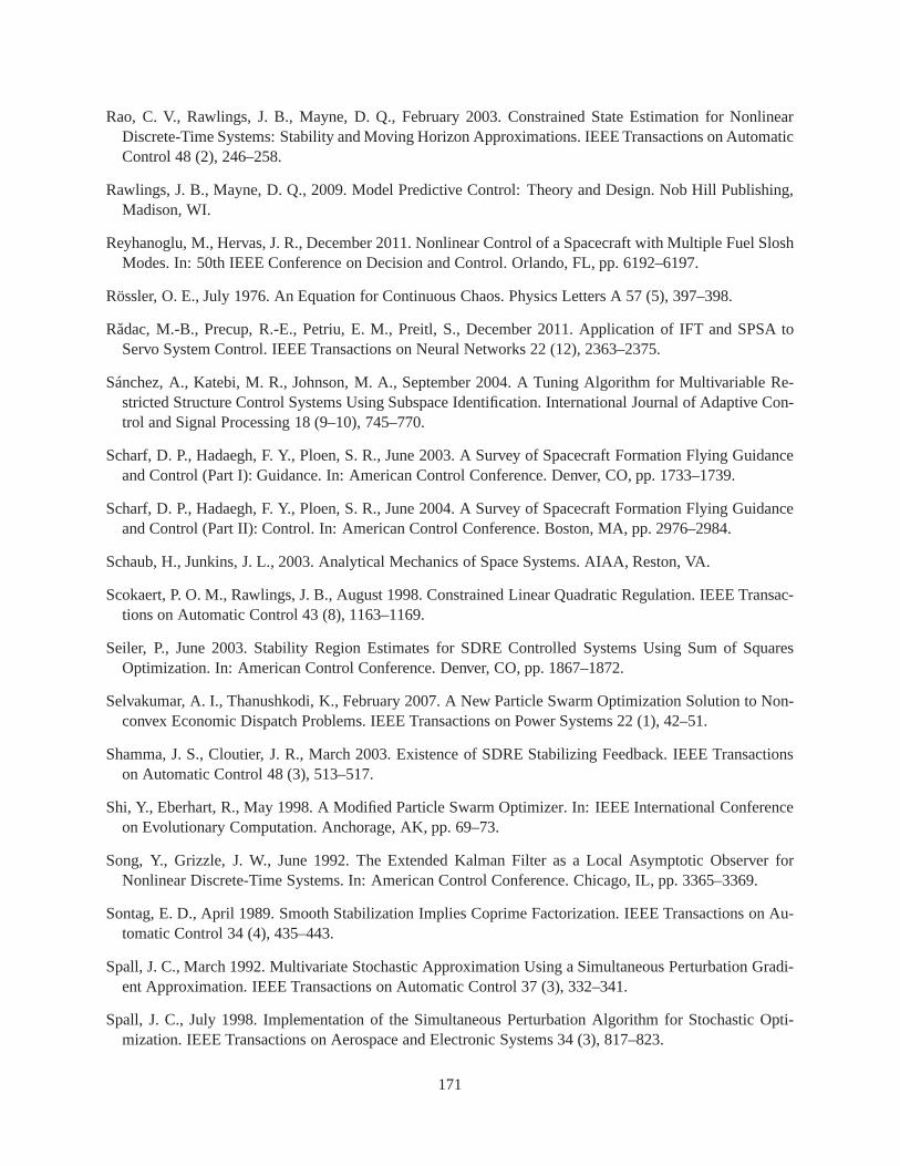
Rao, C. V., Rawlings, J. B., Mayne, D. Q., February 2003. Constrained State Estimation for NonlinearDiscrete-Time Systems: Stability and Moving Horizon Approximations. IEEE Transactions on AutomaticControl 48 (2), 246–258.
Rawlings, J. B., Mayne, D. Q., 2009. Model Predictive Control: Theory and Design. Nob Hill Publishing,Madison, WI.
Reyhanoglu, M., Hervas, J. R., December 2011. Nonlinear Control of a Spacecraft with Multiple Fuel SloshModes. In: 50th IEEE Conference on Decision and Control. Orlando, FL, pp. 6192–6197.
Rössler, O. E., July 1976. An Equation for Continuous Chaos.Physics Letters A 57 (5), 397–398.
Radac, M.-B., Precup, R.-E., Petriu, E. M., Preitl, S., December 2011. Application of IFT and SPSA toServo System Control. IEEE Transactions on Neural Networks22 (12), 2363–2375.
Sánchez, A., Katebi, M. R., Johnson, M. A., September 2004. ATuning Algorithm for Multivariable Re-stricted Structure Control Systems Using Subspace Identification. International Journal of Adaptive Con-trol and Signal Processing 18 (9–10), 745–770.
Scharf, D. P., Hadaegh, F. Y., Ploen, S. R., June 2003. A Survey of Spacecraft Formation Flying Guidanceand Control (Part I): Guidance. In: American Control Conference. Denver, CO, pp. 1733–1739.
Scharf, D. P., Hadaegh, F. Y., Ploen, S. R., June 2004. A Survey of Spacecraft Formation Flying Guidanceand Control (Part II): Control. In: American Control Conference. Boston, MA, pp. 2976–2984.
Schaub, H., Junkins, J. L., 2003. Analytical Mechanics of Space Systems. AIAA, Reston, VA.
Scokaert, P. O. M., Rawlings, J. B., August 1998. Constrained Linear Quadratic Regulation. IEEE Transac-tions on Automatic Control 43 (8), 1163–1169.
Seiler, P., June 2003. Stability Region Estimates for SDRE Controlled Systems Using Sum of SquaresOptimization. In: American Control Conference. Denver, CO, pp. 1867–1872.
Selvakumar, A. I., Thanushkodi, K., February 2007. A New Particle Swarm Optimization Solution to Non-convex Economic Dispatch Problems. IEEE Transactions on Power Systems 22 (1), 42–51.
Shamma, J. S., Cloutier, J. R., March 2003. Existence of SDREStabilizing Feedback. IEEE Transactionson Automatic Control 48 (3), 513–517.
Shi, Y., Eberhart, R., May 1998. A Modified Particle Swarm Optimizer. In: IEEE International Conferenceon Evolutionary Computation. Anchorage, AK, pp. 69–73.
Song, Y., Grizzle, J. W., June 1992. The Extended Kalman Filter as a Local Asymptotic Observer forNonlinear Discrete-Time Systems. In: American Control Conference. Chicago, IL, pp. 3365–3369.
Sontag, E. D., April 1989. Smooth Stabilization Implies Coprime Factorization. IEEE Transactions on Au-tomatic Control 34 (4), 435–443.
Spall, J. C., March 1992. Multivariate Stochastic Approximation Using a Simultaneous Perturbation Gradi-ent Approximation. IEEE Transactions on Automatic Control37 (3), 332–341.
Spall, J. C., July 1998. Implementation of the SimultaneousPerturbation Algorithm for Stochastic Opti-mization. IEEE Transactions on Aerospace and Electronic Systems 34 (3), 817–823.
171

Spong, M. W., Block, D. J., December 1995. The Pendubot: A Mechatronic System for Control Researchand Education. In: 34th IEEE Conference on Decision and Control. New Orleans, LA, pp. 555–556.
Stefanutti, W., Mattavelli, P., Saggini, S., Ghioni, M., January 2007. Autotuning of Digitally ControlledDC–DC Converters Based on Relay Feedback. IEEE Transactions on Power Electronics 22 (1), 199–207.
Stengel, R. F., 1994. Optimal Control and Estimation. DoverPublications, New York, NY.
Suzuki, S., Furuta, K., Sugiki, A., Hatakeyama, S., September 2004. Nonlinear Optimal Internal ForcesControl and Application to Swing-up and Stabilization of Pendulum. Journal of Dynamic Systems, Mea-surement, and Control 126 (3), 568–573.
Tan, K. K., Ferdous, R., Huang, S., August 2002. Closed-LoopAutomatic Tuning of PID Controller forNonlinear Systems. Chemical Engineering Science 57 (15), 3005–3011.
Trelea, I. C., March 2003. The Particle Swarm Optimization Algorithm: Convergence Analysis and Param-eter Selection. Information Processing Letters 85 (6), 317–325.
Vaddi, S. S., Menon, P. K., Ohlmeyer, E. J., March–April 2009. Numerical State-Dependent Riccati Equa-tion Approach for Missile Integrated Guidance Control. AIAA Journal of Guidance, Control, and Dy-namics 32 (2), 699–703.
Vallado, D. A., 2007. Fundamentals of Astrodynamics and Applications, 3rd Edition. Microcosm Press,Hawthorne, CA.
van der Merwe, R., Doucet, A., de Freitas, N., Wan, E., August2000. The Unscented Particle Filter. Tech.Rep. CUED/F-INFENG/TR-380, Cambridge University Engineering Department.
Vreeburg, J. P. B., June 2005. Spacecraft Maneuvers and Slosh Control. IEEE Control Systems Magazine25 (3), 12–16.
Widrow, B., Stearns, P. N., 1985. Adaptive Signal Processing. Prentice Hall, Englewood Cliffs, NJ.
Xin, M., Balakrishnan, S. N., December 2002. A New FilteringTechnique for a Class of Nonlinear Systems.In: 41st IEEE Conference on Decision and Control. Las Vegas,NV, pp. 1034–1039.
Xu, G., Wang, D., September–October 2008. Nonlinear Dynamic Equations of Satellite Relative MotionAround an Oblate Earth. AIAA Journal of Guidance, Control, and Dynamics 31 (5), 1521–1524.
Zhang, S., Taft, C. W., Bentsman, J., Hussey, A., Petrus, B.,September 2012. Simultaneous Gains Tuningin Boiler/Turbine PID-Based Controller Clusters Using Iterative Feedback Tuning Methodology. ISATransactions 51 (5), 609–621.
Zhang, S., Ye, D., Bentsman, J., Taft, C., Hussey, A., June 2010. Assessment of Global Optimizers: ParticleSwarm Optimization, Simulated Annealing, and Genetic Algorithms in Local Simultaneous Multi-LoopTuning of PID Gains. In: 53rd ISA Power Industry Division Symposium. Vol. 483. Summerlin, NV, pp.246–281.
Zhao, X., Lin, Z., December 2008. On the Horizons in Constrained Linear Quadratic Regulation. Automat-ica 44 (12), 3107–3112.
Zhou, K., Doyle, J. C., Glover, K., 1996. Robust and Optimal Control. Prentice Hall, Upper Saddle River,NJ.
172


