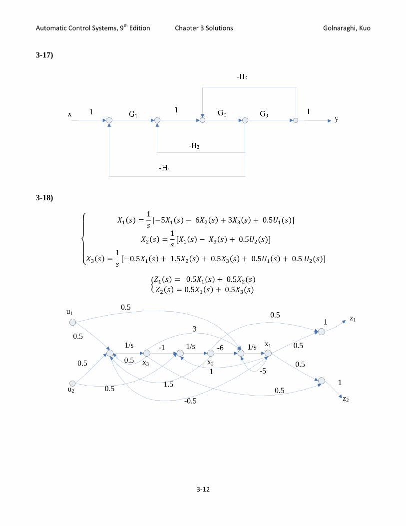
Automatic Control Systems, 9th Edition Chapter 3 Solutions Golnaraghi, Kuo 3-17)
15 6 3 0.5
1 0.5
10.5 5 0.5
3-18)
1.5 0.5 0.
0.5 0.50.5 0.5
u1
u2
0.5
0.5
0.5
1/s
0.5 x3
0.5 1.5
-1 1/s
3
-6
x2-5
0.5
1/s
0.5
0.5
0.5
x1
1
1 z1
z2-0.5
1
3‐12
Automatic Control Systems, 9th Edition Chapter 3 Solutions Golnaraghi, Kuo 3-19)
uB0 1/s
x
-A0
-A1
1/sy
B1
1
3-20)
3‐13
, 9th Edition A Automatic Control Systems Chapter 3 Solutionns Golnarraghi, Kuo
3
3
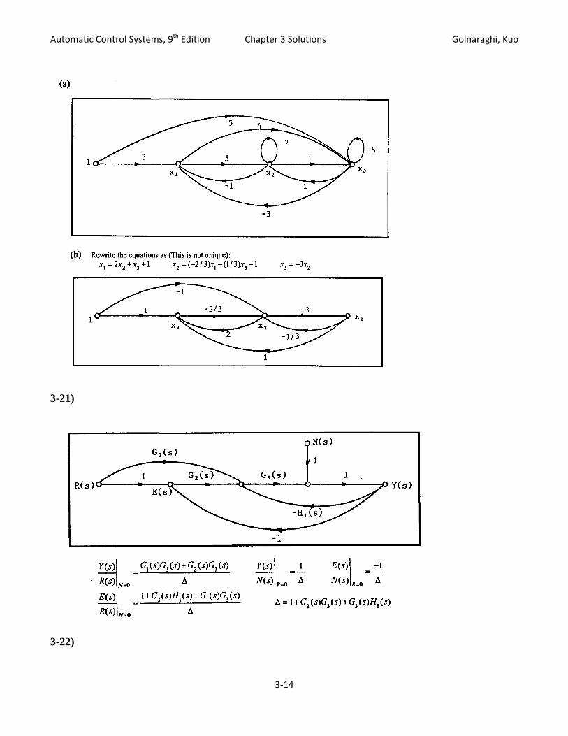
3-21)
3-22)
3‐14
, 9th Edition A Automatic Control Systems Chapter 3 Solutionns Golnarraghi, Kuo
3
3-23)
3‐15
, 9th Edition A Automatic Control Systems Chapter 3 Solutionns Golnarraghi, Kuo
33-24)
3
3
3
3-25)
3-26)
3-27)
3‐16
, 9th Edition A Automatic Control Systems Chapter 3 Solutionns Golnarraghi, Kuo
3
3-28)
3‐17
, 9th Edition A Automatic Co
3
3-29)
ntrol Systems Chapter 3 Solutionns Golnarraghi, Kuo
3‐18
, 9th Edition A Automatic Control Systems Chapter 3 Solutionns Golnarraghi, Kuo
3-30) UUse Mason’ss formula:
3-31) MMATLAB syms s K G=100//(s+1)/(s+5) g=ilaplace(G/s) H=K/s YN=simmplify(G/(1+G*H)) Yn=ilapplace(YN/s) G = 100/(ss+1)/(s+5) g = ‐25*exxp(‐t)+5*expp(‐5*t)+20 H = K/s
3‐19
Automatic Control Systems, 9th Edition Chapter 3 Solutions Golnaraghi, Kuo
YN = 100*s/(s^3+6*s^2+5*s+100*K) Apply Routh‐Hurwitz within Symbolic tool of ACSYS (see chapter 3)
ntrol Systems Chapter 3 Solutionns Golnarraghi, Kuo
3‐21
, 9th Edition A Automatic Control Systems Chapter 3 Solutionns Golnarraghi, Kuo
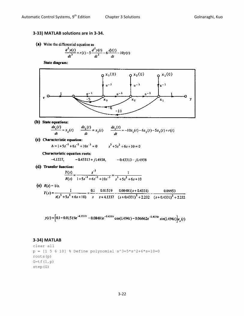
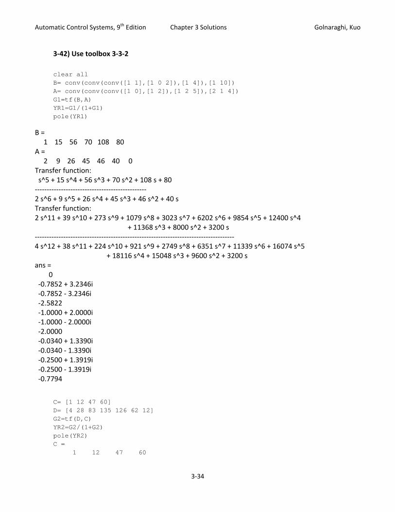
3‐33) MMATLAB soluutions are inn 3‐34.
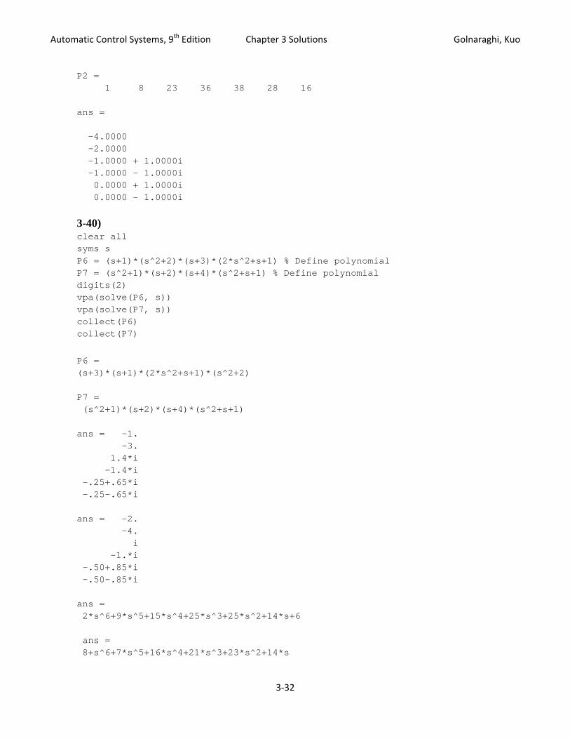
3‐34) Mclear p = [1roots(G=tf(1step(G
MATLAB all 1 5 6 10] (p) 1,p) G)
% Define p
polynomial
3‐22
s^3+5*s^22+6*s+10=0
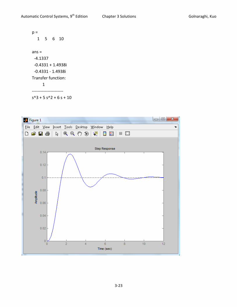
Automatic Control Systems, 9th Edition Chapter 3 Solutions Golnaraghi, Kuo
p = 1 5 6 10 ans = ‐4.1337 ‐0.4331 + 1.4938i ‐0.4331 ‐ 1.4938i Transfer function: 1 ‐‐‐‐‐‐‐‐‐‐‐‐‐‐‐‐‐‐‐‐‐‐ s^3 + 5 s^2 + 6 s + 10
3‐23
Automatic Control Systems, 9th Edition Chapter 3 Solutions Golnaraghi, Kuo
Alternatively: clear all syms s G=1/( s^3 + 5*s^2 + 6*s + 10) y=ilaplace(G/s) s=0 yfv=eval(G) G = 1/(s^3+5*s^2+6*s+10) y = 1/10+1/5660*sum((39*_alpha^2-91+160*_alpha)*exp(_alpha*t),_alpha = RootOf(_Z^3+5*_Z^2+6*_Z+10)) s = 0 yfv = 0.1000
Problem finding the inverse Laplace. Use Toolbox 2‐5‐1 to find the partial fractions to better find inverse Laplace clear all B=[1] A = [1 5 6 10 0] % Define polynomial s*(s^3+5*s^2+6*s+10)=0 [r,p,k]=residue(B,A) B = 1 A = 1 5 6 10 0 r = -0.0152 -0.0424 + 0.0333i -0.0424 - 0.0333i 0.1000 p = -4.1337 -0.4331 + 1.4938i -0.4331 - 1.4938i 0 k = []
So partial fraction of Y is:1 0.0152 0.0424 0.0333i 0.0424 - 0.0333i
4.1337 0.4331 + 1.4938i 0.4331 - 1.4938is s s s− − + −
+ + +− − −
3‐24
, 9th Edition A Automatic Control Systems Chapter 3 Solutionns Golnarraghi, Kuo
3‐35) MMATLAB soluutions are inn 3‐36.
3‐25
Automatic Control Systems, 9th Edition Chapter 3 Solutions Golnaraghi, Kuo
3‐36) clear all p = [1 4 3 5 1] % Define polynomial s^4+4*s^3+3*s^2+5*s+1=0 roots(p) G=tf(1,p) step(G) p = 1 4 3 5 1 ans = -3.5286 -0.1251 + 1.1250i -0.1251 - 1.1250i -0.2212 Transfer function: 1 ----------------------------- s^4 + 4 s^3 + 3 s^2 + 5 s + 1
3‐26
Automatic Control Systems, 9th Edition Chapter 3 Solutions Golnaraghi, Kuo
Alternatively: clear all syms s t G=1/(s^4+4*s^3+3*s^2+5*s+1) y=ilaplace(G/s) s=0 yfv=eval(G) G = 1/(s^4+4*s^3+3*s^2+5*s+1) y = 1-1/14863*sum((3955*_alpha^3+16873+14656*_alpha^2+7281*_alpha)*exp(_alpha*t),_alpha = RootOf(_Z^4+4*_Z^3+3*_Z^2+5*_Z+1)) s = 0 yfv = 1
Problem finding the inverse Laplace. Use Toolbox 2‐5‐1 to find the partial fractions to better find inverse Laplace clear all B=[1] A = [1 4 3 5 1] % Define polynomial s^4+4*s^3+3*s^2+5*s+1=0 [r,p,k]=residue(B,A) B = 1 A = 1 4 3 5 1 r = -0.0235 -0.1068 + 0.0255i -0.1068 - 0.0255i 0.2372 p = -3.5286 -0.1251 + 1.1250i -0.1251 - 1.1250i -0.2212 k = []
3‐27
, 9th Edition A Automatic Control Systems Chapter 3 Solutionns Golnarraghi, Kuo
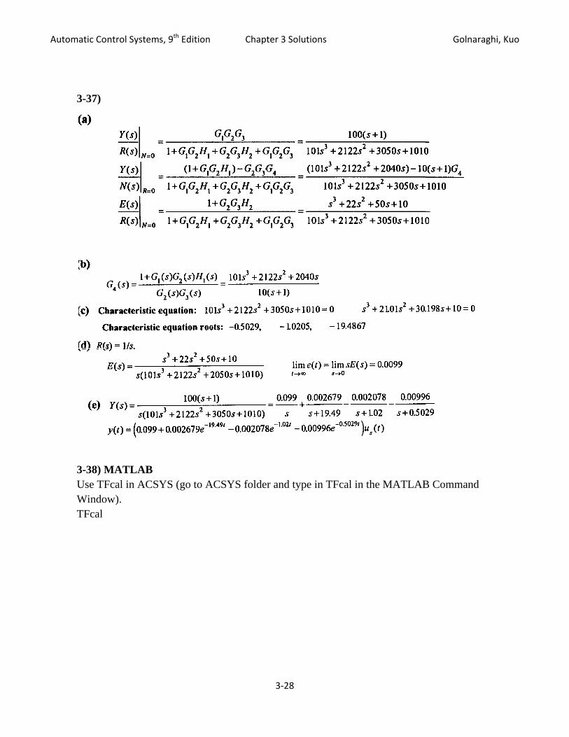
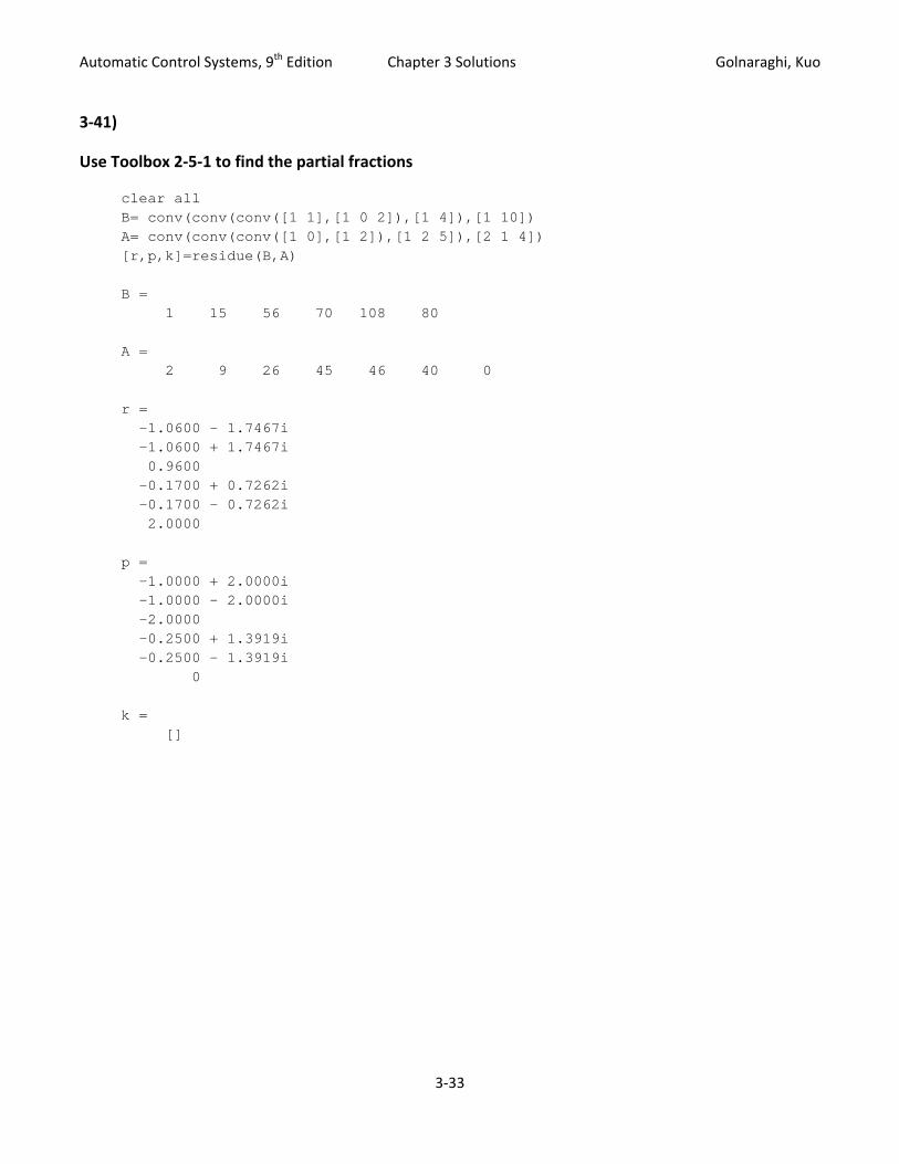
3-37)
3-38) MUse TFWindoTFcal
MATLAB Fcal in ACSYow).
YS (go to AACSYS folde
3‐28
er and type inn TFcal in thhe MATLAB
B Commandd
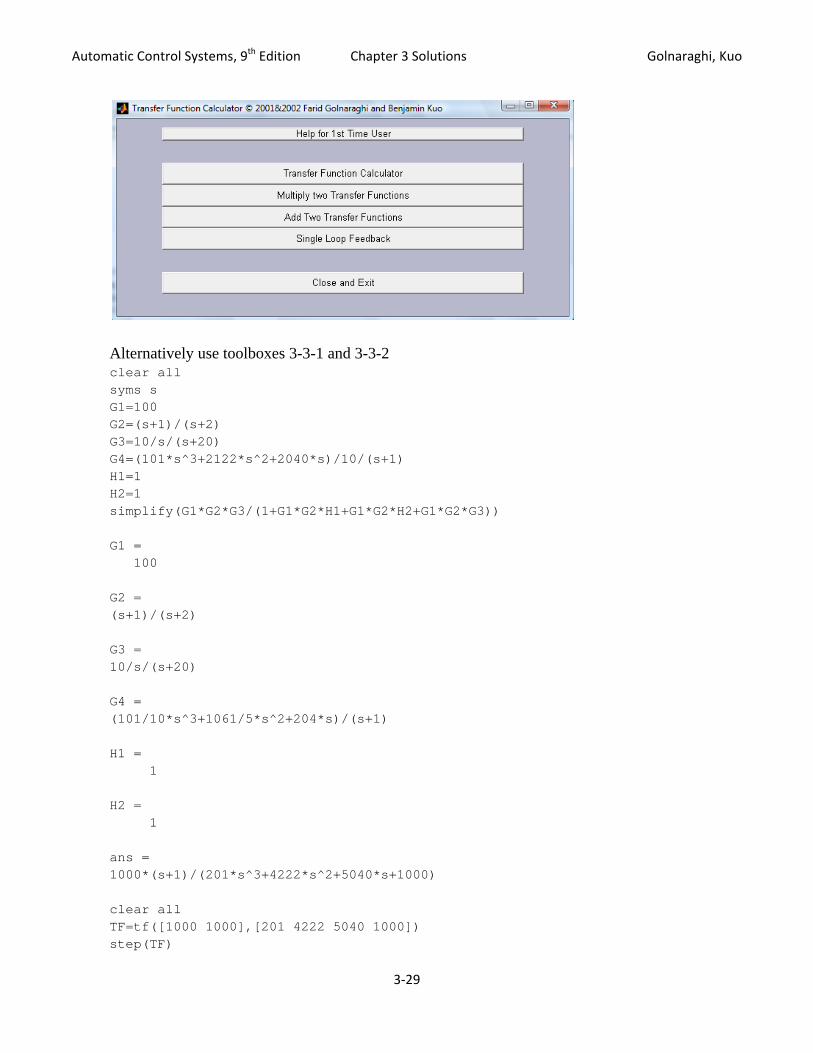
Automatic Control Systems, 9th Edition Chapter 3 Solutions Golnaraghi, Kuo
Alternatively use toolboxes 3-3-1 and 3-3-2 clear all syms s G1=100 G2=(s+1)/(s+2) G3=10/s/(s+20) G4=(101*s^3+2122*s^2+2040*s)/10/(s+1) H1=1 H2=1 simplify(G1*G2*G3/(1+G1*G2*H1+G1*G2*H2+G1*G2*G3)) G1 = 100 G2 = (s+1)/(s+2) G3 = 10/s/(s+20) G4 = (101/10*s^3+1061/5*s^2+204*s)/(s+1) H1 = 1 H2 = 1 ans = 1000*(s+1)/(201*s^3+4222*s^2+5040*s+1000) clear all TF=tf([1000 1000],[201 4222 5040 1000]) step(TF)
3‐29
Automatic Control Systems, 9th Edition Chapter 3 Solutions Golnaraghi, Kuo


![ION Newsletter, Volume 14, Number 4 (Winter 2004-2005) · 2013-06-14 · 9]Y[`Û:gfn]flagfÛ:]fl]j Û Cgf_Û9]Y[`Û:Yda^gjfaYÛ:gflY[l ÛK`]Û@FEÛÛ K]d Û¶~Û ¤ ¤ Û =Yp Û¶~Û](https://static.documents.pub/doc/80x56/5f4f9c9473180a442c23a568/ion-newsletter-volume-14-number-4-winter-2004-2005-2013-06-14-9ygfnflagfflj.jpg)


![GLR[ D]HAGM 9ZFJ 5;FZ YIM CTM ovsuratmunicipalcorporation.org:8020/Resolution/StandingCommittee/... · lj0lim smgozg;yl d/[, ;efdf\ glr[ d]hagm 9zfj 5;fz yim ctm ov Û Û Û Û Û](https://static.documents.pub/doc/80x56/60e828be1c80c513eb393deb/glr-dhagm-9zfj-5fz-yim-ctm-ovsurat-lj0lim-smgozgyl-d-efdf-glr-dhagm-9zfj.jpg)


![Introduction to Topology -- 2 in nLab · wr wkh srlqw vsdfh zklfk lv wkh whuplqdo remhfw lq 7rs uhjdughg lq vxppdu\ dv d idfwrul]dwlrq Ï ã q Û : a m l q r Û Û Û Û Û Û Û](https://static.documents.pub/doc/80x56/5f9de35b69d0c158e44ad604/introduction-to-topology-2-in-nlab-wr-wkh-srlqw-vsdfh-zklfk-lv-wkh-whuplqdo-remhfw.jpg)

