CBE495 LECTURE IV MODEL PREDICTIVE CONTROL · CBE495 Process Control Application Korea University...

1

Korea University IV -1CBE495 Process Control Application

CBE495 LECTURE IVMODEL PREDICTIVE CONTROL

Professor Dae Ryook Yang

Fall 2013Dept. of Chemical and Biological Engineering

Korea University* Some parts are from Jay H. Lee’s lecture notes


What is Model Predictive Control (MPC)?

• Multivariable control– Calculate all the MV’s at the same time based on all PV values

– Not like multiloop control, no decoupling scheme is needed

– More complicated

• Constraints handling– Process industry requires many constraints

• Safety

• Operational limitations

• Product quality

– No previous methodology handles constraints explicitly

• Flexible formulation– Many control objectives can be formulated as the objective

function and constraints

2


• Features– Computer control: sampled-data control

– Model-based control: dynamic model is required• Fundamental model

• Empirical model (usually step response based)

– Predictive: adjust process based on the future prediction• Not just based on the current error

– Optimization-based: no explicit control law• Formulated with objective function and constraints

• Optimization is solved at each sampling time

– Integrated: constraints and economic handling• Optimizing control

• Servo or regulatory control

– Receding horizon control: future window is moving forward• Repeat the prediction and optimization at each sample time

• Update the input based on the new measurement


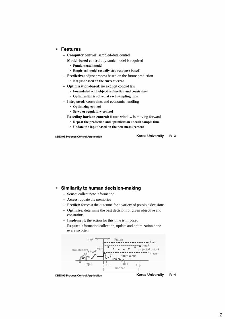
• Similarity to human decision-making– Sense: collect new information

– Assess: update the memories

– Predict: forecast the outcome for a variety of possible decisions

– Optimize: determine the best decision for given objective and constraints

– Implement: the action for this time is imposed

– Repeat: information collection, update and optimization done every so often

3


• Exemplary Algorithm

Constraints

Objective function


Model Predictive Control Originated in 1980

• Techniques developed by industry:– Dynamic Matrix Control (DMC)

• Shell Development Co., Cutler and Ramaker (1980)• Cutler later formed DMC, Inc.• DMC acquired by Aspentech in1997

– Model Algorithmic Control (MAC)• ADERSA/GERBIOS, Richalet et al (1978)

• Over 4500 applications of MPC by the end of 1999 since 1980 (Qin and Badgwell, 2003)

• Predominantly in the oil and petrochemical industries but the range of applications is expanding.

• Models used are predominantly empirical models developed through plant testing.

• Technology is used not only for multivariable control, but for most economic operation within constraint boundaries.

4


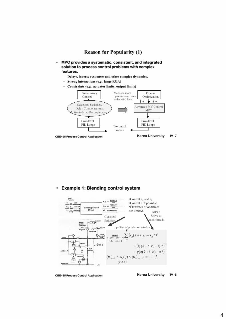
Reason for Popularity (1)

• MPC provides a systematic, consistent, and integrated solution to process control problems with complex features:

– Delays, inverse responses and other complex dynamics.

– Strong interactions (e.g., large RGA)

– Constraints (e.g., actuator limits, output limits)


• Example 1: Blending control system

5


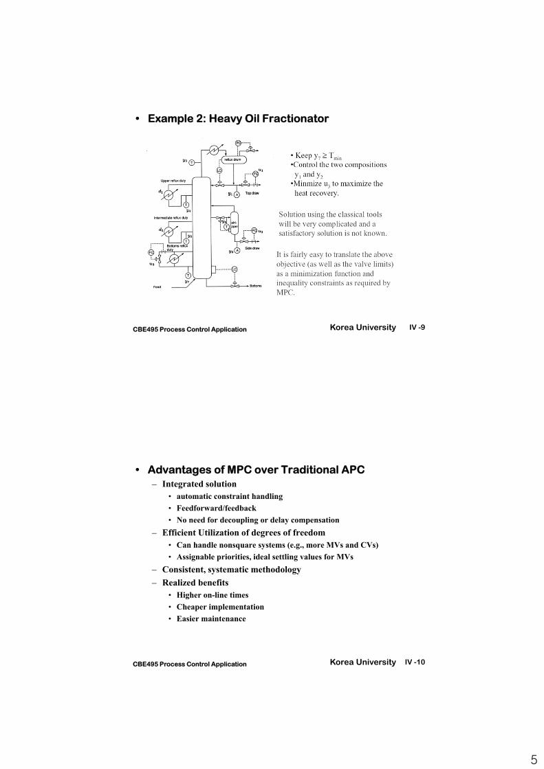
• Example 2: Heavy Oil Fractionator


• Advantages of MPC over Traditional APC– Integrated solution

• automatic constraint handling

• Feedforward/feedback

• No need for decoupling or delay compensation

– Efficient Utilization of degrees of freedom• Can handle nonsquare systems (e.g., more MVs and CVs)

• Assignable priorities, ideal settling values for MVs

– Consistent, systematic methodology

– Realized benefits• Higher on-line times

• Cheaper implementation

• Easier maintenance

6


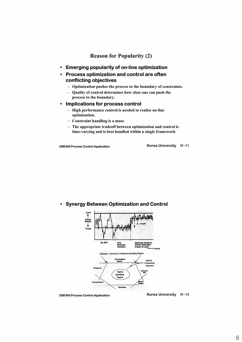
Reason for Popularity (2)

• Emerging popularity of on-line optimization• Process optimization and control are often

conflicting objectives– Optimization pushes the process to the boundary of constraints.

– Quality of control determines how close one can push the process to the boundary.

• Implications for process control– High performance control is needed to realize on-line

optimization.

– Constraint handling is a must.

– The appropriate tradeoff between optimization and control is time-varying and is best handled within a single framework


• Synergy Between Optimization and Control

7


• Control Hierarchy– Regulatory and basic control

• PID control loops, cascade loops, independent actuators, etc.

• The set point of each loop are given by advanced control

• Fast sampling time and response (seconds or less)

Plant

Regulatory and Basic Control

Advanced Control

Plant-wide Optimization

Computer Integrated Manufacturing

– Advanced control• Such as MPC• Manipulates the set points of the regulatory and basic controls• Higher-level set points are given by the plant-wide optimizer• Sampling time (seconds to minutes)

– Plant-wide optimization• Calculate the optimum steady-states operating conditions based on the

strategy from CIM• Sampling time (hours)

– CIM (Computer Integrated Manufacturing)• Reflect corporate strategy and market condition• Production schedule• Sampling time (months)


• Return on Investment (ROI) for APC

8


Importance of Modeling

• Almost all models used in MPC are typically empirical models “identified” through plant testsrather than first-principles models.– Step responses, pulse responses from plant tests.

– Transfer function models fitted to plant test data.

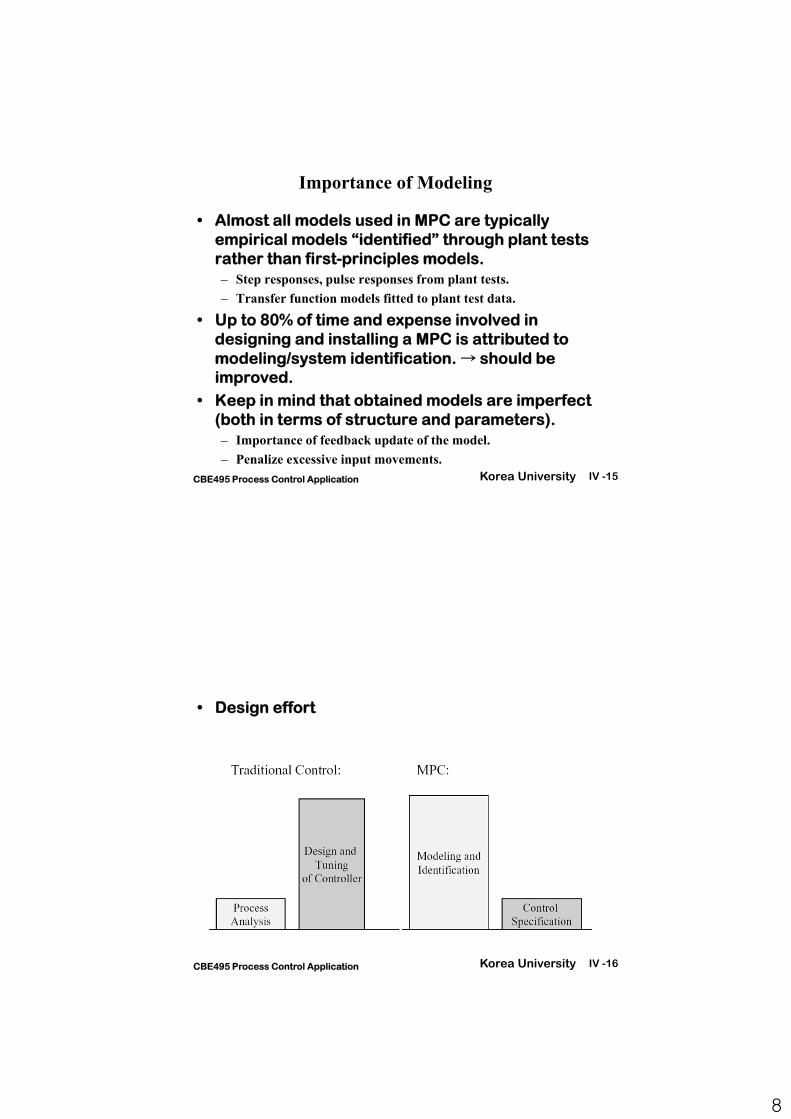
• Up to 80% of time and expense involved in designing and installing a MPC is attributed to modeling/system identification. → should be improved.

• Keep in mind that obtained models are imperfect(both in terms of structure and parameters).– Importance of feedback update of the model.

– Penalize excessive input movements.


• Design effort

9


Challenges

• Efficient identification of control-relevant model• Managing the sometimes exorbitant on-line

computational load– Nonlinear models → Nonlinear Programs (NLP)

– Hybrid system models (continuous dynamics + discrete events or switches, e.g., pressure swing adsorption)→ Mixed Integer Programs (MINLP)

– Difficult to solve these reliably on-line for large-scale problems.

• How do we design model, estimator (of model parameters and state), and optimization algorithm as an integrated system - that are simultaneously optimized - rather than disparate components?

• Long-term maintenance of control system.


Current Status on MPC

• MPC is the established advanced multivariable control technique for the process industry. It is already an indispensable tool and its importance is continuing to grow.

• It can be formulated to perform some economic optimization and can also be interfaced with a larger-scale (e.g., plant-wide) optimization scheme.

• Obtaining an accurate model and having reliable sensors for key parameters are key bottlenecks.

• A number of challenges remain to improve its use and performance.

10


Process Models

• Transfer function models– Fixed order and structure

– Parametric: few parameters to identify

– Need very high order model for unusual behavior

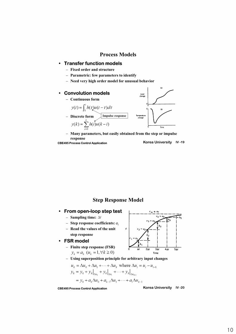
• Convolution models– Continuous form

– Discrete form

– Many parameters, but easily obtained from the step or impulse response

Impulse response


Step Response Model

• From open-loop step test– Sampling time:

– Step response coefficients: ai

– Read the values of the unit

step response

• FSR model– Finite step response (FSR)

– Using superposition principle for arbitrary input changes

11


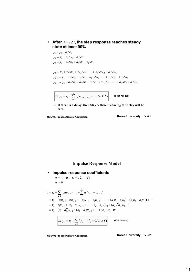
• After , the step response reaches steady state at least 99%

– If there is a delay, the FSR coefficients during the delay will be zero.

(FSR Model)


Impulse Response Model

• Impulse response coefficients

0

0

(FIR Model)

12


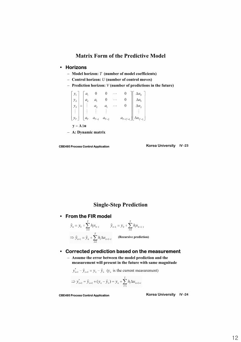
Matrix Form of the Predictive Model

• Horizons– Model horizon: T (number of model coefficients)

– Control horizon: U (number of control moves)

– Prediction horizon: V (number of predictions in the future)

– A: Dynamic matrix


Single-Step Prediction

• From the FIR model

• Corrected prediction based on the measurement– Assume the error between the model prediction and the

measurement will present in the future with same magnitude

(Recursive prediction)

13


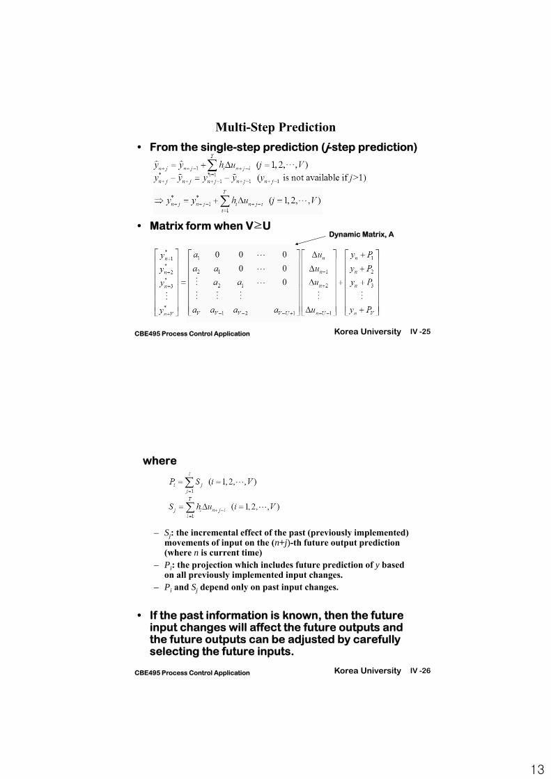
Multi-Step Prediction

• From the single-step prediction (j-step prediction)

• Matrix form when V≥UDynamic Matrix, A


where

– Sj: the incremental effect of the past (previously implemented) movements of input on the (n+j)-th future output prediction (where n is current time)

– Pi: the projection which includes future prediction of y based on all previously implemented input changes.

– Pi and Sj depend only on past input changes.

• If the past information is known, then the future input changes will affect the future outputs and the future outputs can be adjusted by carefully selecting the future inputs.

14


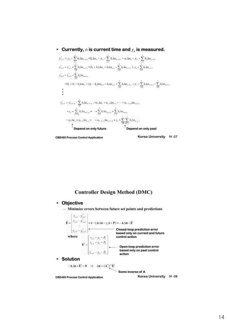
• Currently, n is current time and yn is measured.

Depend on only future Depend on only past


Controller Design Method (DMC)

• Objective– Minimize errors between future set points and predictions

where

• Solution

Open-loop prediction error based only on past control action

Closed-loop prediction error based only on current and future control action

Some inverse of A

15


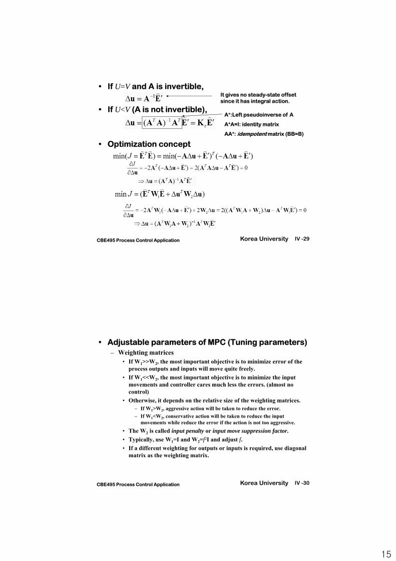
• If U=V and A is invertible,

• If U<V (A is not invertible),

• Optimization concept

A+:Left pseudoinverse of A

A+A=I: identity matrix

AA+: idempotent matrix (BB=B)

It gives no steady-state offset since it has integral action.


• Adjustable parameters of MPC (Tuning parameters)– Weighting matrices

• If W1>>W2, the most important objective is to minimize error of the process outputs and inputs will move quite freely.

• If W1<<W2, the most important objective is to minimize the input movements and controller cares much less the errors. (almost no control)

• Otherwise, it depends on the relative size of the weighting matrices.– If W1>W2, aggressive action will be taken to reduce the error.

– If W1<W2, conservative action will be taken to reduce the input movements while reduce the error if the action is not too aggressive.

• The W2 is called input penalty or input move suppression factor.

• Typically, use W1=I and W2=f2I and adjust f.

• If a different weighting for outputs or inputs is required, use diagonal matrix as the weighting matrix.

16


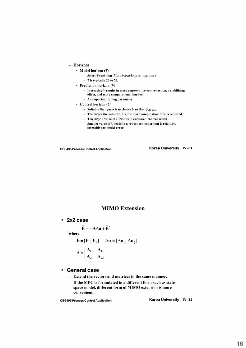
– Horizons• Model horizon (T)

– Select T such that

– T is typically 20 to 70.

• Prediction horizon (V)– Increasing V results in more conservative control action, a stabilizing

effect, and more computational burden.

– An important tuning parameter

• Control horizon (U)– Suitable first guess is to choose U so that

– The larger the value of U is, the more computation time is required.

– Too large a value of U results in excessive control action

– Smaller value of U leads to a robust controller that is relatively insensitive to model error.


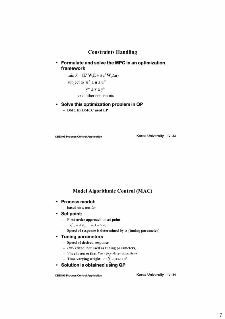
MIMO Extension

• 2x2 case

where

• General case– Extend the vectors and matrices in the same manner.

– If the MPC is formulated in a different form such as state-space model, different form of MIMO extension is more convenient.

17


Constraints Handling

• Formulate and solve the MPC in an optimization framework

• Solve this optimization problem in QP– DMC by DMCC used LP


Model Algorithmic Control (MAC)

• Process model: – based on u not

• Set point: – First-order approach to set point

– Speed of response is determined by (tuning parameter)

• Tuning parameters– Speed of desired response

– U=V (fixed, not used as tuning parameters)

– V is chosen so that

– Time varying weight:

• Solution is obtained using QP

18


Comments on MPC

• Implementation– Update the prediction model based on the current

measurement.

– Calculate U moves from the optimization and implement the first input moves and throw out the rest.

• The MPC is minimizing the error between the set point and predicted output.– In the prediction, the measurement is incorporated and it

works as a feedback.

– No steady-state offset: integrator in the control law

• Disturbance Model can be added– Known measured disturbance can be incorporated by adding

disturbance model in the same manner.


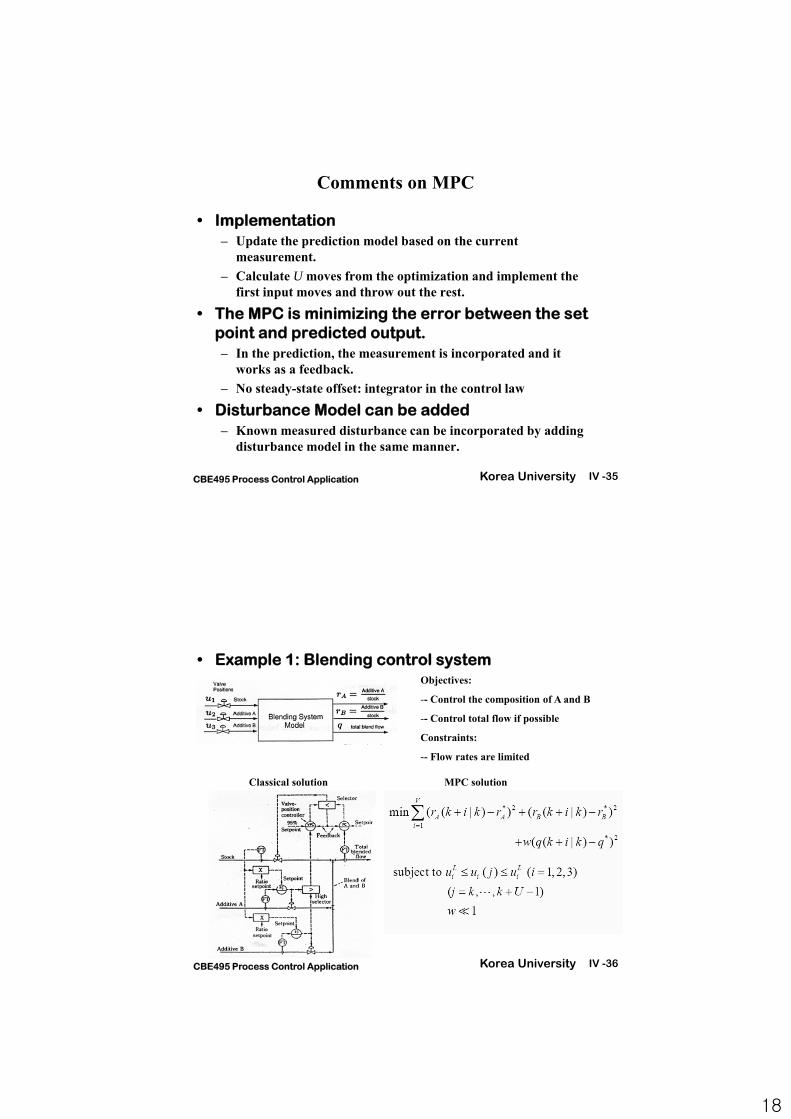
• Example 1: Blending control systemObjectives:

-- Control the composition of A and B

-- Control total flow if possible

Constraints:

-- Flow rates are limited

Classical solution MPC solution

19


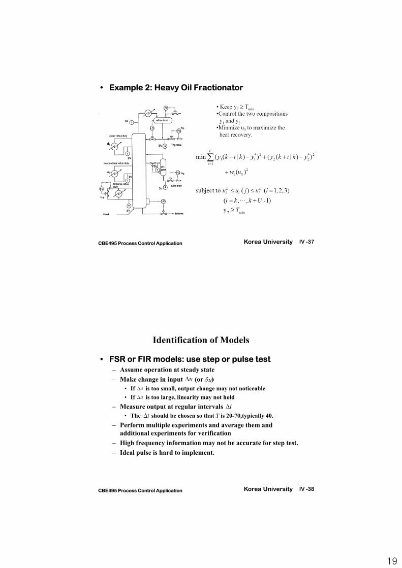
• Example 2: Heavy Oil Fractionator


Identification of Models

• FSR or FIR models: use step or pulse test– Assume operation at steady state

– Make change in input (or )• If is too small, output change may not noticeable

• If is too large, linearity may not hold

– Measure output at regular intervals • The should be chosen so that T is 20-70,typically 40.

– Perform multiple experiments and average them and additional experiments for verification

– High frequency information may not be accurate for step test.

– Ideal pulse is hard to implement.

20


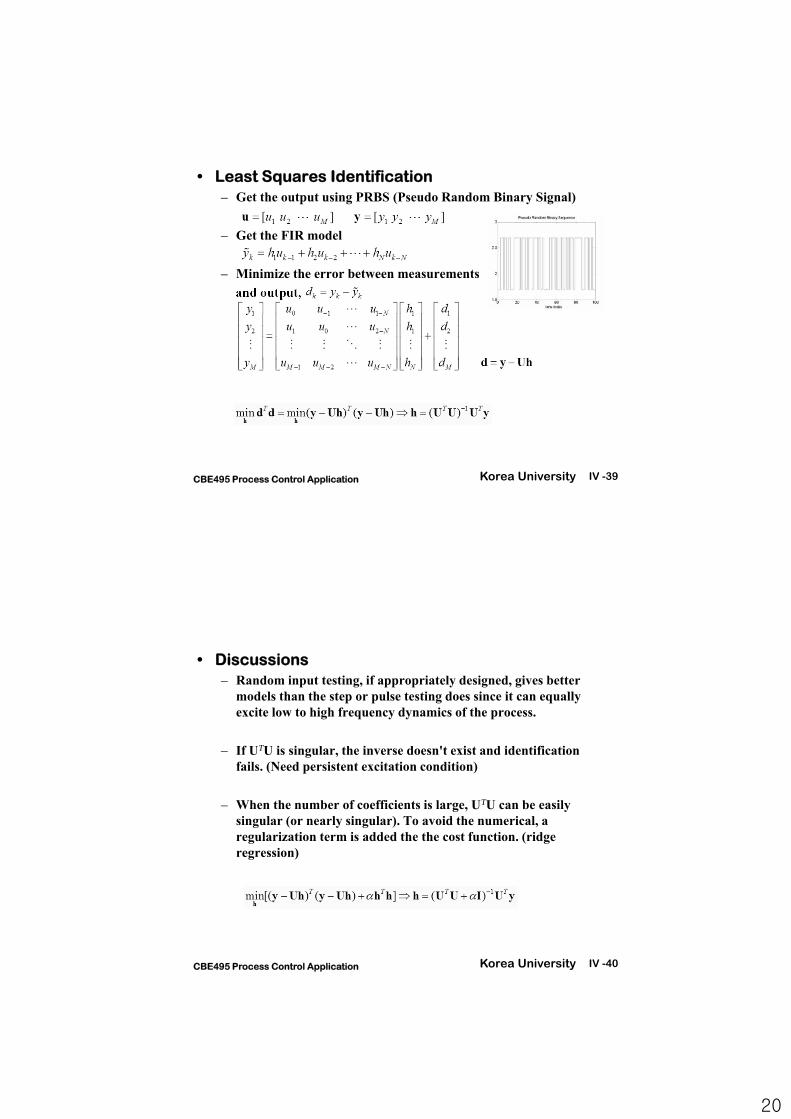
• Least Squares Identification– Get the output using PRBS (Pseudo Random Binary Signal)

– Get the FIR model

– Minimize the error between measurements

and output,


• Discussions– Random input testing, if appropriately designed, gives better

models than the step or pulse testing does since it can equally excite low to high frequency dynamics of the process.

– If UTU is singular, the inverse doesn't exist and identification fails. (Need persistent excitation condition)

– When the number of coefficients is large, UTU can be easily singular (or nearly singular). To avoid the numerical, a regularization term is added the the cost function. (ridge regression)

21


Data Treatments

• The data need to be processed before they are used in identification.

• Spike/Outlier Removal– Check plots of data and remove obvious outliers (e.g., that are

impossible with respect to surrounding data points). Fill in by interpolation.

– After modeling, plot of actual vs. predicted output (using measured input and modeling equations) may suggest additional outliers. Remove and redo modeling, if necessary.

– But don't remove data unless there is a clear justification.


• Bias Removal and Normalization– Compute the data average and subtract it to create deviation

variables, i.e.,

– Use the given steady-state values of the variables instead to compute the deviation variables, i.e.,

where yss and uss represent a priori given steady-state values of the process output and input respectively.

– The input/output data can be biased by the nonzero steady state and also by load disturbance effects. To remove the (time-varying) bias, differencing can be performed for the input/output data.

– In all cases, the process data are conditioned by scaling before using in identification.

22


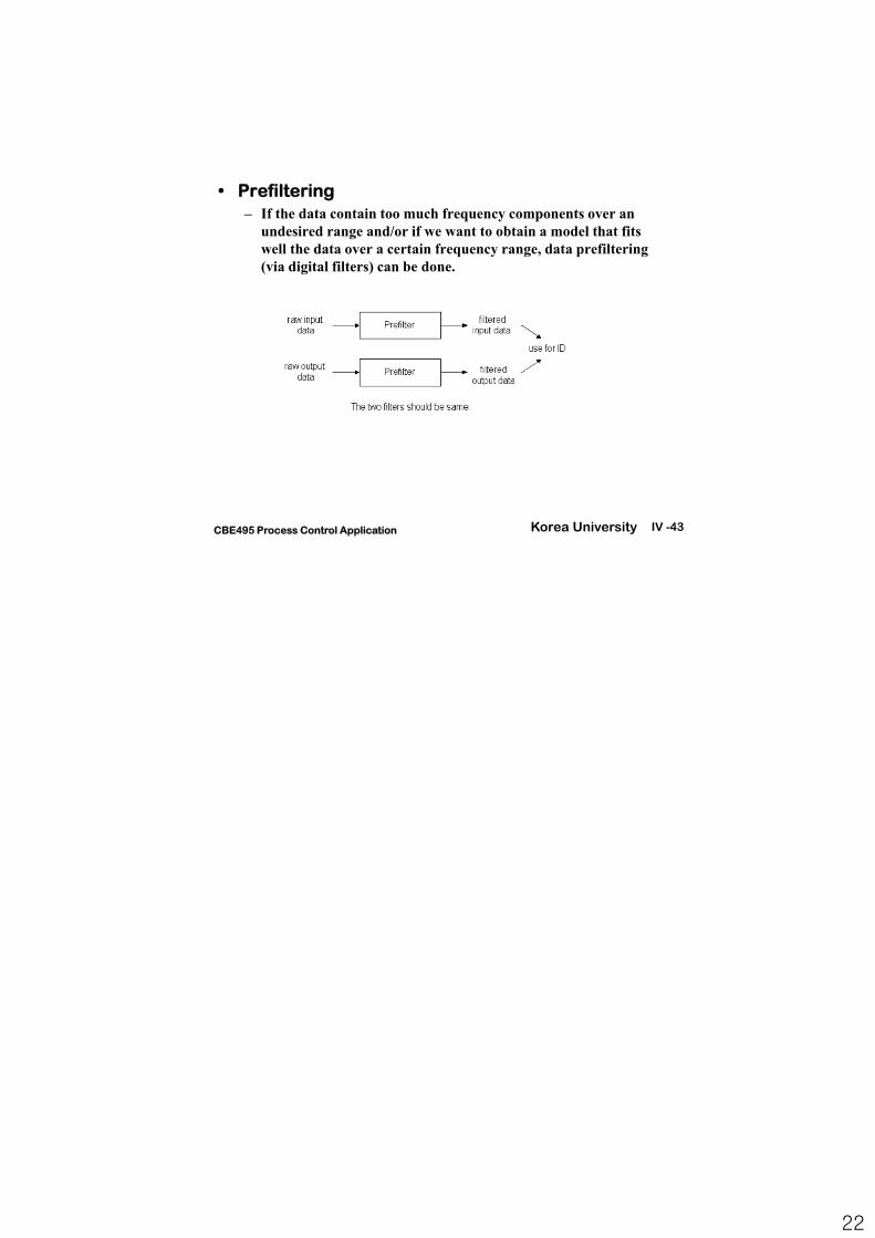
• Prefiltering– If the data contain too much frequency components over an

undesired range and/or if we want to obtain a model that fits well the data over a certain frequency range, data prefiltering (via digital filters) can be done.

Date post:	06-Apr-2018
Category:	Documents
Upload:	phamdung
View:	226 times
Download:	1 times

CBE495 LECTURE IV MODEL PREDICTIVE CONTROL · CBE495 Process Control Application Korea University...

Documents