CFD Modelling of an evaporative Cooling System Andres Pinilla, Jorge López, Hugo Pineda, Miguel Asuaje, Nicolás Ratkovich Chemical Engineering Department Universidad de los Andes. Colombia 1
Transcript
CFD Modelling of an evaporative Cooling System
Andres Pinilla, Jorge López, Hugo Pineda, Miguel Asuaje, Nicolás Ratkovich
Chemical Engineering Department
Universidad de los Andes. Colombia
1
Content
• Introduction• Cooling by fogging system
• Objectives
• Methodology • Cases of Study
• Results
• Conclusions
• Future Work
2
Introduction
3
Turbines that work in hot weathers
Lower performance at higher temperatures
Cooling system
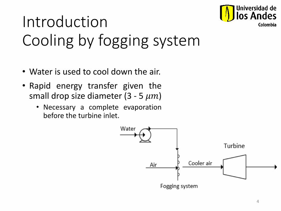
IntroductionCooling by fogging system
• Water is used to cool down the air.
• Rapid energy transfer given thesmall drop size diameter (3 - 5 𝜇𝑚)• Necessary a complete evaporation
before the turbine inlet.
4
Objectives
CFD modeling of an evaporative cooling system.
• To validate the results found in the simulation with reportedexperimental results.
• To study the heat and mass transfer in the duct.
• To investigate the water droplets behavior in terms ofagglomeration and fractionation.
8Figure 1: Duct geometry where the cooling occurs (in mm).
ResultsHeat Transfer
9
0
5
10
15
20
25
30
35
0 0.5 1 1.5 2
Tem
per
atu
re(°
C)
Time (s)Experimento Simulación
0
5
10
15
20
25
30
35
0 0.5 1 1.5 2
Tem
per
atu
re(°
C)
Time (s)
Experimento Simulación
0
5
10
15
20
25
30
35
0 0.5 1 1.5 2
Tem
per
atu
re(°
C)
Time (s)
Experimento Simulación
0
5
10
15
20
25
30
35
0 0.5 1 1.5 2
Tem
per
atu
re(°
C)
Time (s)
Experimento Simulación
Figure 2: Results for temperature for each case
ResultsHeat Transfer (cont…)
10
Case Experiment
temperature (°C)
Simulation
temperature (°C)
Difference (%)
A 15.50 16.09 3.82
B 15.34 16.33 6.44
C 23.76 24.73 4.06
D 23.53 24.97 6.12
Figure 3: a) Lateral contour plot of temperature. b) Up contour plot of temperature
ResultsHeat Transfer (cont…)
11
ResultsMass Transfer
12
40
50
60
70
80
90
100
0 0.5 1 1.5 2
Rel
ativ
eh
um
idit
y(%
)
Time (s)
Experimento Simulación
40
50
60
70
80
90
100
0 0.5 1 1.5 2
Rel
ativ
eh
um
idit
y(%
)
Time (s)
Experimento Simulación
0
20
40
60
80
100
0 0.5 1 1.5 2
Rel
ativ
eh
um
idit
y(%
)
Time (s)
Experimento Simulación
0
20
40
60
80
100
0 0.5 1 1.5 2
Rel
ativ
eh
um
idit
y(%
)
Time (s)
Experimento Simulación
Figure 4: Results of relative humidity for case: a) A. b) B, c) C, d) D
ResultsMass Transfer (cont…)
The exact position on the sensors was not clearly specified, this can be a possible cause of error.
13
Case Experiment (%) Simulation (%) Difference %
A 96.00 91.87 4.30
B 95.90 88.74 7.46
C 96.51 92.07 4.59
D 95.66 95.66 7.07
Figure 5: Distribution of the sensors across the duct
ResultsVolume Fraction of Water
14
Figure 6: a) Liquid volume fraction of water a) Lateral view y b) Upside view
ResultsParticle Diameter
After the reduction zone, the droplet size reduces faster, as expected
15
Figure 7: Water droplets diameter
0
1
2
3
4
5
6
7
0 0.5 1 1.5 2
Dia
met
er(μ
m)
Time (s)20HR 50μm 60HR 50μm
Conclusions
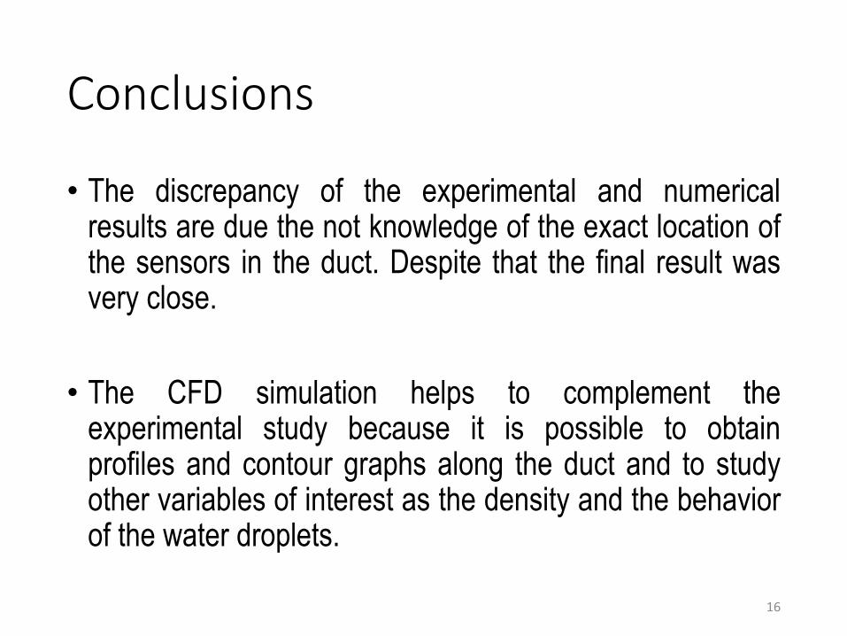
• The discrepancy of the experimental and numericalresults are due the not knowledge of the exact location ofthe sensors in the duct. Despite that the final result wasvery close.
• The CFD simulation helps to complement theexperimental study because it is possible to obtainprofiles and contour graphs along the duct and to studyother variables of interest as the density and the behaviorof the water droplets.
16
Conclusions & Future Work
• It is recommended to use nozzles that atomize water with a particlediameter of 20 𝜇𝑚, and with the lowest relative humidity.
• Using CFD tool it is possible to identify where can exist corrosionproblems and also it is possible to modify the geometry in order toimprove the mass and heat transfer.
17Figure 8: Corrosion problem in the duct
CFD Modelling of an evaporative Cooling System
Andres Pinilla, Jorge López, Hugo Pineda, Miguel Asuaje, Nicolás Ratkovich