CFD SIMULATION OF A SMALL STIRLING …

CFD SIMULATION OF A SMALL STIRLING CFD SIMULATION OF A SMALL STIRLING CFD SIMULATION OF A SMALL STIRLING CFD SIMULATION OF A SMALL STIRLING

CRYOCOOLERCRYOCOOLERCRYOCOOLERCRYOCOOLER A THESIS SUBMITTED IN PARTIAL FULFILLMENTA THESIS SUBMITTED IN PARTIAL FULFILLMENTA THESIS SUBMITTED IN PARTIAL FULFILLMENTA THESIS SUBMITTED IN PARTIAL FULFILLMENT OF THE REQUIREMENTS FOR THE DEGREE OFOF THE REQUIREMENTS FOR THE DEGREE OFOF THE REQUIREMENTS FOR THE DEGREE OFOF THE REQUIREMENTS FOR THE DEGREE OF Bachelor of TechnologyBachelor of TechnologyBachelor of TechnologyBachelor of Technology InInInIn Mechanical EngineeringMechanical EngineeringMechanical EngineeringMechanical Engineering ByByByBy AMRIT AMRIT AMRIT AMRIT BIKRAM SAHUBIKRAM SAHUBIKRAM SAHUBIKRAM SAHU ROLL NOROLL NOROLL NOROLL NO---- 10603032106030321060303210603032 Under the gUnder the gUnder the gUnder the guiduiduiduidance ofance ofance ofance of Prof. R.K. SAHOOProf. R.K. SAHOOProf. R.K. SAHOOProf. R.K. SAHOO Department of Mechanical EngineeringDepartment of Mechanical EngineeringDepartment of Mechanical EngineeringDepartment of Mechanical Engineering National Institute of TechnologyNational Institute of TechnologyNational Institute of TechnologyNational Institute of Technology, , , , RourkelaRourkelaRourkelaRourkela

2010

This is to certify that the project entitled “CFD Simulation of a small Stirling Cryocoolers”,

being submitted by Mr. Amrit Bikram Sahu, in the partial fulfillment of the requirement

for the award of the degree of B. Tech in Mechanical Engineering, is a

research carried out by him at the Department of Mechanical Engineering, National Institute

of Technology Rourkela, under our guidance and supervision.

To the best of my knowledge, the matter embodied in the thesis has not been sub

other University / Institute for the award of any Degree or Diploma.

Date:

CERTIFICATE

that the project entitled “CFD Simulation of a small Stirling Cryocoolers”,


for the award of the degree of B. Tech in Mechanical Engineering, is a


of Technology Rourkela, under our guidance and supervision.

To the best of my knowledge, the matter embodied in the thesis has not been sub

other University / Institute for the award of any Degree or Diploma.

Prof. R. K. Sahoo

Dept. of Mechanical Engineering

National Institute of Technology

Rourkela- 769008

that the project entitled “CFD Simulation of a small Stirling Cryocoolers”,


record of bonafide


To the best of my knowledge, the matter embodied in the thesis has not been submitted to any

Prof. R. K. Sahoo

Mechanical Engineering

ational Institute of Technology

769008

ACKNOWLEDGEMENT

I would like to express my sincere gratitude to my guide Prof. R. K. Sahoo for his invaluable

guidance and steadfast support during the course of this project work. Fruitful and

rewarding discussions with him on numerous occasions have made this work possible. It has

been a great pleasure for me to work under his guidance.

I am also indebt to Mr. Ezaz Ahmed, M. Tech, Dept. of Mechanical Engineering, for his

constant support and encouragement during the numerical simulations which has made this work

possible. I would also like to express my sincere thanks to all the faculty members of Mechanical

Engineering Department for their kind co-operation. I would like to acknowledge the

assistance of all my friends in the process of completing this work.

Finally, I express my sincere gratitude to my parents for their constant encouragement and

support.

Amrit Bikram Sahu

Roll No.: 10603032

Dept. of Mechanical Engineering

NIT Rourkela

CONTENTS

Abstract i

List of figures ii

CHAPTER 1 INTRODUCTION 1

1.1 Cryocoolers 2

1.2 Types of cryocoolers 2

1.3 Applications of cryocoolers 5

1.4 Stirling cryocooler 6

CHAPTER 2 LITERATURE SURVEY 11

2.1 Earlier models of cryocoolers developed 12

2.2 Literature review of simulations of Stirling

cryocoolers 13

CHAPTER 3 COMPUTATIONAL FLUID DYNAMICS 15

3.1 Computational fluid dynamics 16

3.2 Fluent & Gambit 20

CHAPTER 4 RESULTS & DISCUSSIONS 28

4.1 No load case with frequency of 30Hz 29

4.2 Comparison of cooling behavior in no load case

and 0.5W load case 36

4.3 Determining the optimum frequency 37

CHAPTER 5 CONCLUSION 38

REFERENCES 40

ABSTRACT

The application of cryocoolers has skyrocketed due to various necessities of modern day

applications such as adequate refrigeration at specified temperature with low power input, long

lifetime, high reliability and maintenance free operation with minimum vibration and noise,

compactness and light weight. The demand of Stirling cryocoolers has increased due to the

ineffectiveness of Rankine cooling systems at lower temperatures. With the rise in applications

of Stirling cryocoolers, especially in the field of space and military, several simulations of

Stirling cryocoolers were developed. These simulations provided an edge to the developers, as it

could provide an accurate analysis of the performance of the cryocooler before actually

manufacturing it. This saved a lot of time and money. In this project, an attempt has been made

to develop a CFD simulation of a small Stirling cryocooler. A detailed analysis has been done of

the simulation of the cryocooler in the results and discussion section. A comparison has also

been made between the cooling curves in no load and a 0.5W load case. An attempt has also

been made in determining the optimum frequency of operation of the proposed model of Stirling

cryocooler by comparing the minimum cool down temperature attained by them.

i

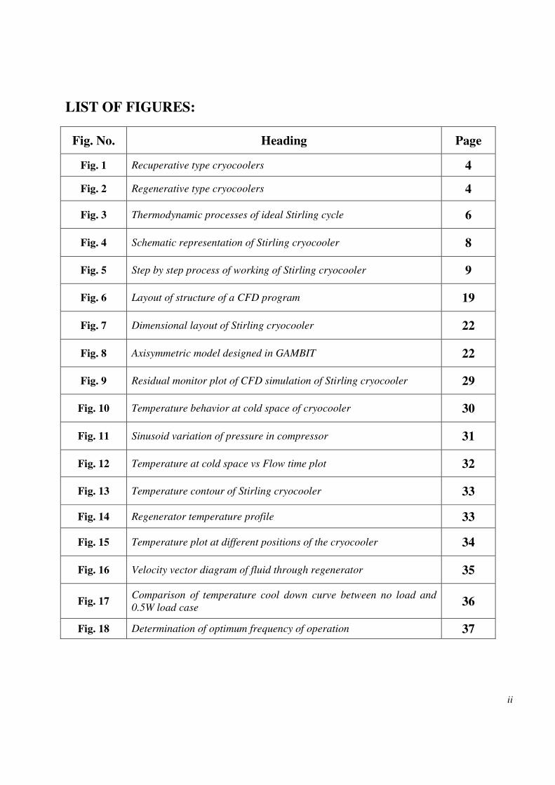
LIST OF FIGURES:

Fig. No. Heading Page

Fig. 1 Recuperative type cryocoolers 4

Fig. 2 Regenerative type cryocoolers 4

Fig. 3 Thermodynamic processes of ideal Stirling cycle 6

Fig. 4 Schematic representation of Stirling cryocooler 8

Fig. 5 Step by step process of working of Stirling cryocooler 9

Fig. 6 Layout of structure of a CFD program 19

Fig. 7 Dimensional layout of Stirling cryocooler 22

Fig. 8 Axisymmetric model designed in GAMBIT 22

Fig. 9 Residual monitor plot of CFD simulation of Stirling cryocooler 29

Fig. 10 Temperature behavior at cold space of cryocooler 30

Fig. 11 Sinusoid variation of pressure in compressor 31

Fig. 12 Temperature at cold space vs Flow time plot 32

Fig. 13 Temperature contour of Stirling cryocooler 33

Fig. 14 Regenerator temperature profile 33

Fig. 15 Temperature plot at different positions of the cryocooler 34

Fig. 16 Velocity vector diagram of fluid through regenerator 35

Fig. 17 Comparison of temperature cool down curve between no load and

0.5W load case 36

Fig. 18 Determination of optimum frequency of operation 37

ii

1 | P a g e

CHAPTER 1CHAPTER 1CHAPTER 1CHAPTER 1

INTRODCUTION

2 | P a g e

1.1. CRYOCOOLERS:

Cryocooler can be simply defined as a refrigeration machine that provides refrigeration in a

temperature range of 0K – 150K. Recent development of technologies, especially in the domain

of space and military applications, has significantly increased the application of cryogenics.

1.2. TYPES OF CRYCOCOOLERS:

Cryocoolers can be classified on the basis of types of operating cycle and on the basis of type of

heat exchanger.

1.2.1. Types of operating cycles:

� Open cycle cryocoolers:

These are cryocoolers that use stored cryogens either in subcritical or supercritical liquid state,

solid cryogens or stored as high pressure gas with a Joule- Thomson expansion valve.

� Closed cycle cryocoolers:

Closed cycle cryocoolers provide cooling at cryogenic temperature and reject heat at very high

temperatures. They are also known as mechanical cryocoolers. A few examples are Stirling

cryocoolers, Brayton cycle cryocoolers, closed cycle Joule-Thomson cryocoolers etc.

3 | P a g e

1.2.2. Types of heat exchangers used:

� Recuperative cryocoolers:

These are analogous to DC electrical systems since the direction of flow of the working fluid is

in one direction only. Due to this reason, the compressor and expander have separate inlet and

outlet valves to maintain the flow direction. Valves are necessary unless the system has any

rotary or turbine elements. The performance of these cryocoolers primarily depends upon the

type of working fluid or refrigerant used. One of the main advantages of these cryocoolers is that

it can be scaled to any size ( i.e. even upto the order of few MWs). They can be further classified

into valveless and with valves cryocoolers. A few examples of recuperative cryocoolers can be

seen in Fig.1.

� Regenerative cryocoolers:

These cryocoolers are analogous to AC electrical system since the working fluid oscillates in the

flow channel. The compressor and expander do not need any valves since there is a single flow

channel. The regenerator, which has a very high heat capacity, stores the heat for half a cycle and

then releases it back to the working fluid. These cryocoolers cannot be scaled up to large sizes,

however, these are very efficient because of very low heat transfer loss. Liquid helium is

commonly used as working fluid in these types of cryocoolers. Fig.2 shows a few examples of

regenerative cryocoolers.

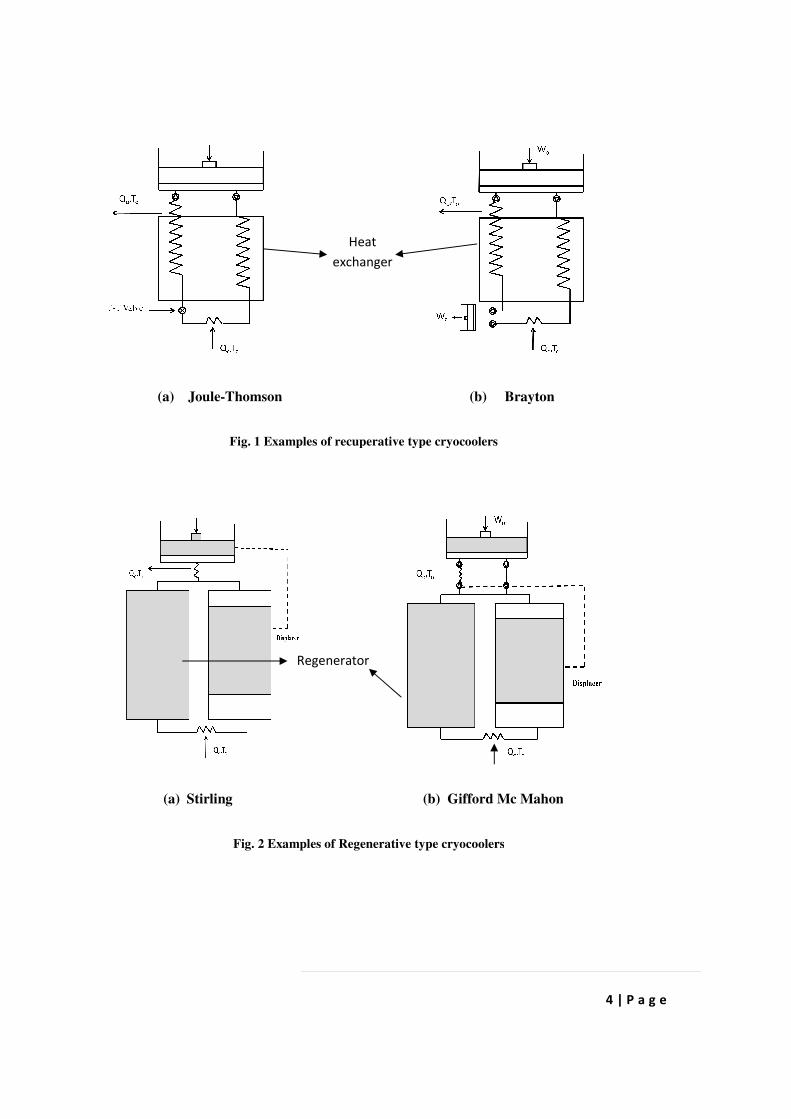
(a) Joule-Thomson

Fig. 1 Examples of recuperative type cryocoolers

(a) Stirling

Fig. 2 Examples of Regenerative type cryocoolers

Thomson (b) Brayton

Examples of recuperative type cryocoolers

(b) Gifford Mc Mahon

Examples of Regenerative type cryocoolers

Regenerator

Heat

exchanger

4 | P a g e

Gifford Mc Mahon

5 | P a g e

1.3. APPLICATIONS OF CRYOCOOLERS:

1.3.1. Military applications:

� IR sensors for missile guidance and night vision

� IR sensors for surveillance( satellite based)

� Gamma ray sensor for monitoring nuclear activity

� Superconducting magnets for mine sweeping

1.3.2. Environmental:

� IR sensors for atmospheric studies(satellite based)

� IR sensors for pollution control.

1.3.3. Medical applications:

� Cooling superconductors for MRI

� Cryosurgery

1.3.4. Commercial applications:

� Cryopumps

� Industrial gas liquefaction

� Cooling superconductors for cellular phone base stations

1.3.5. Transport applications:

� Superconducting magnets for maglev trains

1.4. STIRLING CRYOCOOLER:

Stirling cryocoolers are regenerator type cryocoolers which work on the basis of Stirling cycle.

An ideal Stirling cycle consists of two isothermal process and two const

seen in Fig. 3. The detailed explanation of Stirling cycle has been done in the following section.

1.4.1. Stirling cycle:

Fig. 3 Thermodynamic processes of an ideal Stirling cycle

An ideal Stirling cycle has two isothermal process and two

Fig. 3 shows a reverse Stirling cycle on the basis of which a Stirling refrigerator works.

The Stirling cycle can be explained by four thermodynamic processes.

P

3

4

STIRLING CRYOCOOLER:


An ideal Stirling cycle consists of two isothermal process and two constant volume processes as

. The detailed explanation of Stirling cycle has been done in the following section.

Thermodynamic processes of an ideal Stirling cycle

An ideal Stirling cycle has two isothermal process and two constant volume processes.

shows a reverse Stirling cycle on the basis of which a Stirling refrigerator works.


V

6 | P a g e


ant volume processes as

. The detailed explanation of Stirling cycle has been done in the following section.

constant volume processes.

shows a reverse Stirling cycle on the basis of which a Stirling refrigerator works.


2

1

7 | P a g e

� Isothermal Expansion:

The expansion space and associated heat exchanger are maintained at a constant

temperature while the gas undergoes isothermal expansion owing to the expansion in

volume of the cryocooler.

� Isochoric Heat Addition:

The gas passes through the regenerator where it gains much heat because of lower

enthalpy of gas than the regenerator.

� Isothermal Compression:

The piston compresses the gas and the gas undergoes isothermal compression where

the temperature of compression space and associated heat exchanger are maintained

constant.

� Isochoric Heat Rejection:

The gas passes back through the regenerator, losing heat to it, owing to higher

enthalpy of gas than the regenerator.

1.4.2. Design of Stirling cryocooler:

The layout of a typical Stirling cryocooler has been shown in Fig. 4. The main components of the

Stirling cryocooler are Piston, Compressor space, Aftercooler, Transfer line, Regenerator, Cold

space and Hot space. Piston and Regenerator are the moving components of the cryocooler while

rest is stationary. The Piston and Regenerator follow a reciprocating motion that is achieved by

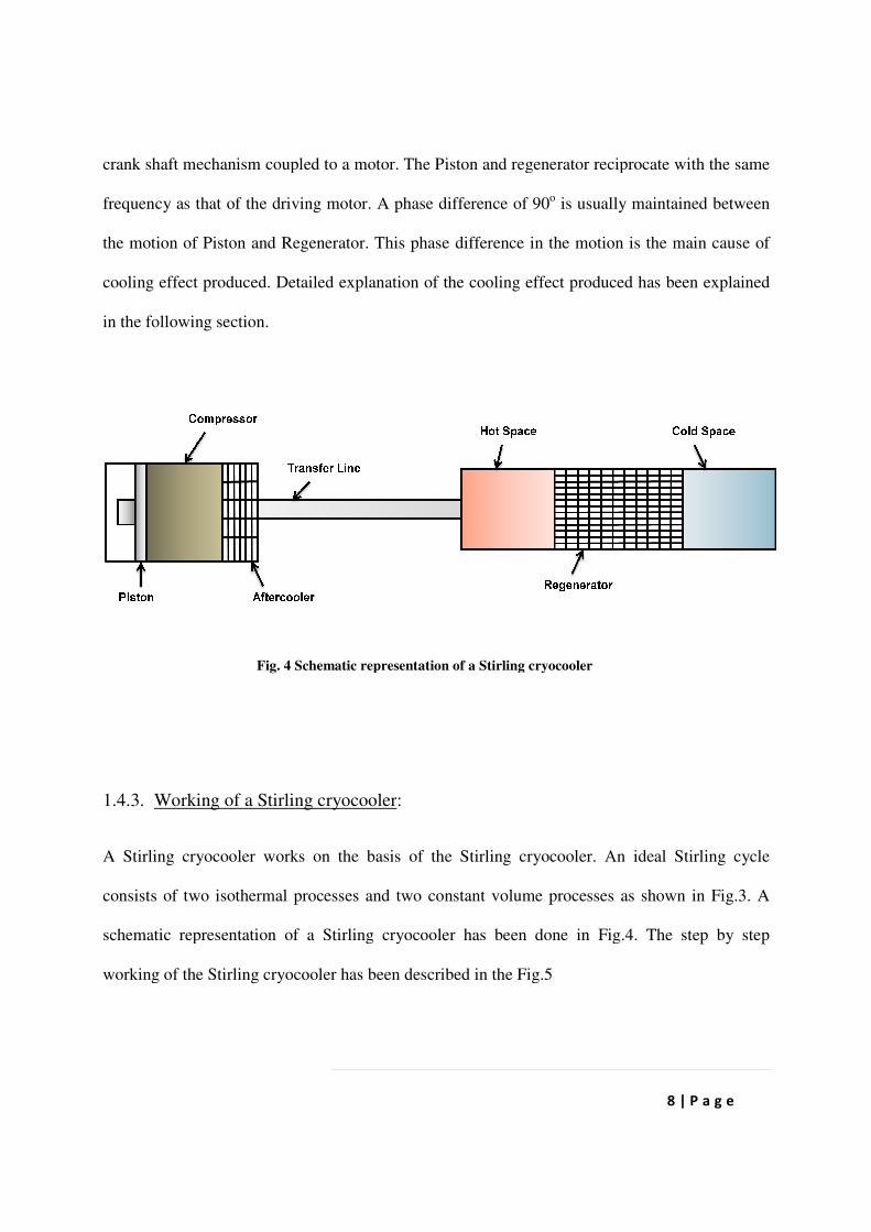
crank shaft mechanism coupled to a motor. The Piston and regenerator reciprocate with the same

frequency as that of the driving motor. A phase difference of 90

the motion of Piston and Regenerator. This phase difference in the motion is the main cause of

cooling effect produced. Detailed explanation of the cooling effect produced

in the following section.

Fig. 4 Schematic representation of a Stirling cryocooler

1.4.3. Working of a Stirling cryocooler

A Stirling cryocooler works on the basis of the Stirling cryocooler. An ideal Stirling cycle

consists of two isothermal processes and two constant volume

schematic representation of a Stirling cryocooler has been done in Fig.

working of the Stirling cryocooler has been described in the Fig.


frequency as that of the driving motor. A phase difference of 90o is usually maintained between


cooling effect produced. Detailed explanation of the cooling effect produced

Schematic representation of a Stirling cryocooler

Working of a Stirling cryocooler:


consists of two isothermal processes and two constant volume processes as shown in Fig.

schematic representation of a Stirling cryocooler has been done in Fig.

working of the Stirling cryocooler has been described in the Fig.5

8 | P a g e


is usually maintained between


cooling effect produced. Detailed explanation of the cooling effect produced has been explained


processes as shown in Fig.3. A

schematic representation of a Stirling cryocooler has been done in Fig.4. The step by step

Fig. 5 Step by step process of the working of a Stirling cryocooler

Let the Stirling cryocooler be in the state of maximum volume at initial time. This position refers

to state 1 in Fig.3. In this state the working fluid is at least pressure and minimum tempera

and is present at the cold space. In the next step, the regenerator moves significantly forcing the

fluid to pass through it while the piston stays almost stationary, thus maintaining a constant

(a)

(b)

(c)

(d)

Step by step process of the working of a Stirling cryocooler

tirling cryocooler be in the state of maximum volume at initial time. This position refers

. In this state the working fluid is at least pressure and minimum tempera



9 | P a g e

tirling cryocooler be in the state of maximum volume at initial time. This position refers

. In this state the working fluid is at least pressure and minimum temperature



10 | P a g e

volume. Since the temperature of the fluid in cold space is lower than the temperature of

regenerator, when the fluid passes through the regenerator it absorbs heat from the regenerator.

Since the volume is almost constant, temperature rises and hence its pressure also rises which

takes it to state 2. This is the constant volume heat addition process. Next the piston moves to

compress the working fluid to minimum volume state and the maximum pressure state while the

regenerator remains almost stationary. The fluid is at maximum temperature and is present in the

hot space now and is in state 3. In the next step, the regenerator moves towards left thus forcing

the hot fluid to flow through it. Since the temperature of the fluid is much higher than the

regenerator temperature, it loses heat to the regenerator mesh and thus there is a decrease in

pressure at constant volume. This is represented by state 4 in the Fig.3 . Now, the piston moves

toward left causing expansion and hence, the temperature of the working fluid reduces and

comes back to state 1. This is the state of minimum temperature. The expansion process causes

the cooling effect. This cycle repeats itself in the Stirling cryocooler to reach a steady state and a

minimum temperature state.

11 | P a g e

CHAPTER CHAPTER CHAPTER CHAPTER 2222

LITERATURE SURVEY

12 | P a g e

2.1. EARLIER MODELS OF CRYOCOOLERS DEVELOPED:

As mentioned in the earlier sections, cryocoolers are now being widely applied in the areas of

infrared detectors, superconductor filters, satellite based applications, Cryopumps etc. Stirling

cryocoolers were introduced to the commercial market in 1950s for the first time as single

cylinder air liquefiers and cryocoolers for IR sensors to about 80K. In early1960s, William Beale

invented free-piston Stirling engines acting as power systems and have been in continuous

development process since then. The first development of linear free-piston Stirling cryocooler

was achieved at Philips laboratories, Eindhoven. Another significant linear Stirling cryocooler

unit was developed by Dr. G. Davey, Oxford University. Oxford-split Stirling cryocooler have

been developed since its invention in Oxford University in the year 1970s which resulted in

developments of many new components such as no contact seals, flexure springs, linear

compressor etc[1]. In an Oxford type Stirling cryocooler, the regenerator always contains a long-

stack of phosphor-bronze discs, frequency of piston and displacer is very high (30 – 60 Hz) and

the oscillating motion of the working fluid is very complicated [2]. Nowadays Oxford-split

Stirling cryocoolers are largely found in space and flight based applications. In 1980, the US

navy started a program, in which new designs for cryocoolers were solicited which would have a

coefficient of performance within a range of 2000 to 10000 W/W. In addition to this, programs

were received from NBS- Boulder where development of a nylon and fiberglass Stirling cycle

cryocooler had begun under ONR support [3]. Over the last few decades, there have been rapid

developments in the field of miniature free piston free displacer Stirling cryocooler. In 1997,

AFRL, Raytheon and JPL together developed flight based Stirling cryocoolers whose operating

range was 25K – 120K. It provided refrigeration upto 3W at 60K and 1.5W at 35K[4]. A light

13 | P a g e

weight linear driven cryocooler was also developed for cryogenically cooled solid state Laser

systems was developed by Decade Optical Systems, Inc. (DOS Inc.) in the year 1997[5]. It has

been ascertained that all mechanical cryocoolers gained a sufficient amount of cooling capacity

with unprecedentedly low amount of power consumption for the cooling requirement of large

telescopes and other applications [6].

4.2.1. LITERATURE REVIEW OF SIMULATIONS OF STIRLING CRYOCOOLERS:

With the rapid development in the cryocooler design and functioning over the past 60 years, it

became highly essential to develop computer based simulations for them. These simulations

could provide a detailed analysis of the cryocooler’s functioning and various characteristics

before actually developing it, which in turn saves a lot of time and money. With this intent, the

work for development of computer based simulations for cryocoolers began. Analysis of the

ideal Stirling cycle was done by Schmidt (first order approach). He made assumptions such as

steady state procedure with ideal regenerators and no pressure drops during the isothermal

processes. The second order approach was largely developed by Martini, in which he further

analyzed by adding realistic losses to the model developed by Schmidt. Realistic losses included

pressure drop loss, shuttle loss, pumping loss, static heat loss, regenerator ineffectiveness [7]. He

applied decoupled independent correction to account for various losses which have been

thoroughly described in Martini’s 1982 Stirling engine design manual [8]. During later half of

the decade, this analysis of Martini was adopted for carrying out Stirling simulations at the

University of Calgary which was later written in FORTRAN 77 language to create an easy to use

digital simulation program for microcomputers, namely CRYOWEISS by Walker et al [7]. This

program was used for predicting results of PPG-1 Stirling liquefier and for comparing it with

experimental results. Under an Independent Research program at Lockheed’s Research and

14 | P a g e

Development Division, a third order split-Stirling refrigerator model was developed. Continuous

System Simulation Language (CSSL) was used for programming the model. The model had 90

nodes, maximum of which were found in the regenerator region [9]. This model was validated

against experimental results for the Lucas Stirling refrigerators, carried out by Yuan et al [10].

Later, a dynamic model of a one-stage Oxford Stirling cryocooler was developed that could

predict the dynamic processes and performances for the given structure dimensions and

operating conditions [1].

A CFD code, CAST (Computer Aided Simulation of Turbulent flows) was developed by Peric

and Scheuerer in 1989, for predicting two-dimensional flow and heat transfer phenomena. The

code was written in FORTRAN IV. This code was used by several Cleveland State University

graduate students to simulate various Stirling machine components. The development process of

the CAST code has been explained in detail by Ibrahim et al [11]. In this case, Fluent has been

used to simulate the Stirling cryocooler problem.

15 | P a g e


COMPUTATIONAL FLUID

DYNAMICS

16 | P a g e

3.1. COMPUTATIONAL FLUID DYNAMICS

3.1.1. Introduction:

During the last three decades, Computational Fluid Dynamics has been an emerged as an

important element in professional engineering practice, cutting across several branches of

engineering disciplines. CFD is concerned with numerical solution of differential equations

governing transport of mass, momentum, and energy in moving fluids. Today, CFD finds

extensive usage in basic and applied research, in design of engineering equipment, and in

calculation of environmental and geophysical phenomena. For a long time, design of various

engineering components like heat exchangers, furnace etc required generation of empirical

information which were very difficult to generate. Another disadvantage of these empirical

information is that, they are applicable for a limited range of scales of fluid velocity temperature

etc. Fortunately, solving differential equations describing mass transport, momentum and energy

and then interpreting the solution to practical design was the key to the whole designing process.

With the advent of computers, these differential equations were solved at a speed that increased

exponentially and hence the applications of CFD became widespread.

17 | P a g e

3.1.2. Governing equations:

The three main governing equations are mentioned below:

� Transport of mass:

� �� 0 (1)

� Momentum equation:

��

��

�� (2)

� Energy equation:

��

��

�� !

""" (3)

3.1.3. Steps in a typical CFD problem:

� The physical domain is specified according to the given flow situation.

� Various boundary conditions, fluid properties are defined and appropriate transport equations

are selected.

� Nodes are defined in the space to map it into the form of a grid and control volumes are

defined around each node.

18 | P a g e

� Differential equations are integrated over a control volume to convert them into an algebraic

one. Some of the popular techniques used for discretization are finite difference method and

finite volume method.

� A numerical method is devised to solve the set of algebraic equations and a computer

program is developed to implement the numerical method.

� The solution is interpreted.

� The results are displayed and post process analysis is done.

CFD can be broadly divided in to 3 elements as shown in Fig. 6:

o Preprocessor:

During preprocessing, the user

• Defines the modeling goals

• Identifies the computational domains

• Designs and creates the grid system

o Main Solver:

The main solver sets up the equations required to compute the flow field according to the various

options and criteria chosen by the user. It also meshes the points created by the preprocessor

which is essential for solving fluid flow problems. The process broadly includes selecting proper

physical model, defining material properties, boundary conditions, operating conditions, setting

up solver controls, limits, initializing solutions, solving equations and finally saving the output

data for post process analysis.

19 | P a g e

o Post processor:

It is the last but a very important part of CFD in which the results of the simulation is examined

and conclusions are drawn. It allows user to plot various data in the form of graphs, contours,

vectors etc. Global parameters like Nusselt number, friction factor Reynolds number etc can be

calculated and data can be exported for better visualizations.

Fig. 6 Layout of the structure of a CFD program

20 | P a g e

3.2. FLUENT & GAMBIT:

3.2.1. Introduction:

Fluent is a computer program that is used for modeling heat transfer and modeling fluid flow in

complex geometries. Due to mesh flexibility offered by Fluent, flow problems with unstructured

meshes can be solved easily. Fluent supports triangular, quadrilateral meshes in 2D problems and

tetrahedral, hexahedral, wedge shaped meshes in 3D.

Fluent has been developed in C language and hence, provides full flexibility and power offered

by the language. C language provides facilities like efficient data structures, flexible solver

controls and dynamic memory allocation also. Client- server architecture in Fluent allows it to

run as separate simultaneous processes on client desktop workstations and computer servers.

This allows efficient execution, interactive control and complete flexibility of the machine.

Fluent provides a interactive menu driven interface. This interface is written in a language called

Scheme, a dialect of LISP. Through this interface, Fluent provides all functions required to

compute the solution and display the results.

User can create geometry and grid using Gambit. The grid formation can be either triangular,

quadrilateral, tetrahedral or a combination of all. Gambit provides flexibility to the user in

generating grid by providing various parameters like interval size, number of grids, or the

shortest edge %. The user has to define the type of edges/faces to be either wall, internal,

velocity inlet etc and the volumes to be either fluid or solid. After creating the geometry and

defining its various parts properly, it is exported to FLUENT for simulations.

21 | P a g e

Once the grid is created by user in Gambit, it is read into Fluent. Fluent performs all the

remaining operations required in order to solve the problem like defining the boundary

conditions, materials for the system, refining the grid, initializing various parameters etc. It also

provides post processing features of the results. Fluent uses unstructured meshes which reduces

the time user spent in generating meshes, simplifies the geometry modeling and mesh generation

process, models more complex geometries than that possible by using multi-block structured

meshes and lets user adapt the mesh to resolve the flow field features. Fluent can handle

triangular and quadrilateral meshes in 2D and tetrahedral, hexahedral, pyramidal and wedge

shaped meshes in 3D space.

3.2.2. Modeling details:

� Gambit:

The geometric modeling and nodalization of various parts of Stirling cryocooler has been done

using GAMBIT. Due to the symmetry of the model, as can be seen in Fig. 7, a 2D axisymmetric

design was developed. Uniform sized quadrilateral meshes has been used to mesh the model as

can be seen in Fig. 8. The main components of the design are Piston, Compressor, Aftercooler,

Transfer line, Hot space, Regenerator, Cold space and Displacer. Piston and displacer are the

only moving parts of the cryocooler while the rest parts are stationary. The dimensions and zone

and boundary setting of the model have been illustrated in Table 1.

22 | P a g e

Fig. 7 A layout of the model of the simulated Stirling cryocooler with its proper dimensions

Fig. 8 Axisymmetric model of the Stirling cryocooler developed in GAMBIT

All units are in mm

23 | P a g e

Sl. No. Components Radius( in mm) Length( in mm)

1. Compressor 8 9

2. Aftercooler 8 3

3. Transfer line 1 55

4. Hot space 5 5

5. Regenerator 5 45

6. Cold space 5 7

7. Piston 8 -

8. Displacer/ Cold Piston 5 -

Table 1. Dimensions of the various components of the proposed model of Stirling cryocooler

� Fluent:

After creating and defining the grid of the model in GAMBIT, the mesh file is read into the main

solver, i.e. FLUENT. The grid is them checked to assure that all the zones are present and all

dimensions are correct. Skewness and swap tests are also done on the grid. Then, a proper scale

is chosen according to the actual model of which simulation is to be done and all the units are

assigned. For this study, the above mentioned grid was scaled by a factor of 0.001 in order to

bring the units to mm.

24 | P a g e

3.2.3. Defining the model:

Before iterating, the model properties such as Fluent solver, materials, thermal and fluid

properties besides model operating conditions and boundary conditions have to be defined to

solve the fluid flow problems. The conditions specified in this case have been mentioned below.

� Solver:

Segregated solver, implicit formulation, axisymmetric space, unsteady time.

� Viscous model and energy equation:

k- epsilon set of equations and energy equation were selected.

� Materials:

Helium (ideal gas) as working fluid and Steel for the frame material.

� Operating conditions:

Operating pressure was chosen to be 101325 Pa.

� Boundary conditions:

Aftercooler and Hot space were chosen to have isothermal walls while rest of the walls were

chosen to be adiabatic with either zero heat flux or a certain heat flux depending upon the case to

be simulated. Aftercooler and regenerator were chosen to be porous zones. The detailed

boundary conditions have been mentioned in the next page.

25 | P a g e

• Piston: The piston was chosen to be an adiabatic wall and it material was steel.

• Compressor: The walls were chosen to be made of steel and were adiabatic. The compressor

space was filled with Helium.

• Aftercooler: The walls were chosen to be isothermal, maintaining a constant temperature of

300K. The interior of aftercooler was chosen to be a porous zone. Details of the porous

medium are given below.

Porosity: 0.69

Viscosity: X: 9.433e+09 1 m%⁄ ; Y: 9.433e+09 1 m%⁄

Inertial resistance: X: 76090 1 m⁄ ; Y: 76090 1 m⁄

The material of the porous zone and the walls was chosen to be steel and the void spaces were

filled with Helium.

• Transfer line: The walls of the transfer line are adiabatic and are made of steel. Its interior is

filled with Helium.

• Hot space: The walls of the hot space are isothermal maintaining a constant temperature of

300K and is made of steel. The hot space is filled with helium.

• Regenerator: The regenerator is chosen to be a porous medium with the following details

.

Porosity: 0.69

Viscosity: X: 9.433e+09 1 m%⁄ ; Y: 9.433e+09 1 m%⁄

Inertial resistance: X: 76090 1 m⁄ ; Y: 76090 1 m⁄

26 | P a g e

The material of the porous zone and the walls was chosen to be steel and the void spaces were

filled with Helium.

• Cold space: The space is filled with Helium and its walls are adiabatic in nature. The material

of the cold space walls is steel.

• Displacer: The displacer is made of steel and is adiabatic in nature.

� Limits:

Pressure: 15atm to 25atm

� Pressure velocity coupling: PISO

� Under relaxation factors:

Pressure: 0.2; Momentum: 0.4; Energy: 0.8

� Discretization:

Pressure: PRESTO

Density, momentum, energy were chosen to be First Order Upwind.

� Convergence criterion for continuity, x-velocity, y-velocity, k was chosen to be 0.001 and

energy was chosen to be 1e-06.

In order to avoid complications and divergence during the iteration process, a complementary

motion was applied to displacer instead of the regenerator which kept the volume of hot space

constant but the volume of cold space varied with time.

27 | P a g e

3.2.4. Defining motions of piston and displacer:

Separate UDFs were written in C language for defining the reciprocating motion for piston and

displacer. These UDFs were built and loaded in Fluent and they were coupled with their

respective zones (piston and displacer in this case). Various parameters like frequency and

amplitude of reciprocating motion could be entered in the UDFs. In order to modify the meshing

of the model to compensate the changes brought due to the reciprocating motion of various parts,

dynamic meshing option was selected in which resmeshing and layering parameters were

defined. In order to verify the motion generated by the UDFs and to determine a proper time

step, mesh motion was done several times before running the actual simulation.

28 | P a g e


RESULTS & DISCUSSIONS

29 | P a g e

Numerous simulations were run by varying different parameters like frequency of reciprocating

motion, boundary conditions etc and comparing the results to find an optimum condition. No

changes were brought in the design of the cryocooler during the simulation processes. Four cases

of no load condition were run with frequencies of 20 Hz, 30Hz, 40Hz and 50 Hz. No load

condition represents a case where no heat flux is given at the cold end of the cryocooler. One

more case was run, in which a load of 0.5W was applied at the cold end condition. The results

have been shown and discussed in the following sections.

4.1. NO LOAD CASE WITH FREQUENCY OF 30HZ:

A simulation of the Stirling cryocooler was run. The frequency of reciprocating motion of the

piston and displacer was specified to be 30Hz. No heat flux was applied to the cold end of the

Stirling cryocooler. The residual monitor plot for the above simulation is shown in Fig. 9. The

residual monitor shows no signs of divergence.

Fig. 9 Residual monitor plot of a CFD simulation of Stirling cryocooler

30 | P a g e

4.1.1. Cooling behavior:

Fig. 10 shows the trend of decrease in temperature at the cold end. The temperature is observed

to follow a gradually descending sinusoidal wave.

Fig. 10 Sinusoid behavior of temperature at cold space of the cryocooler

4.1.2. Pressure behavior:

Fig. 11 clearly shows the sinusoidal variation of pressure in compressor space generated mainly

due to the reciprocating motion of the piston.

31 | P a g e

Fig. 11 Sinusoidal pressure variation at the compressor end during a simulation

4.1.3. Cooling curve:

The temperature of the cold end begins to drop initially at a greater slope initially but gradually

the slope decreases and the system reaches a steady state. The cooling curve can be seen in

Fig.12 The simulation was run for 172.5 seconds.

32 | P a g e

Fig. 12 Temperature vs Flow time plot in a simulation of Stirling cryocooler with no load condition,

frequency: 30 Hz, phase difference: 900

4.1.4. Temperature contour:

The temperature gradient in the Stiring cryocooler after 172.4 seconds of simulation can be seen

in Fig. 13. The highest temperature is observed at compressor end while the lowest temperature

is observed at the cold end of the cryocooler. The temperature profile of the regenerator, whose

ends are marked by red vertical lines, can be clearly observed in Fig. 14. The temperature on the

left side of the regenerator is higher and it gradually decreases linearly as we move towards right

(i.e. towards the cold space).

Fig. 13 Temperature contour of the Stirling cryocooler with no load condition, frequency: 30Hz, phase

Fig.

Temperature contour of the Stirling cryocooler with no load condition, frequency: 30Hz, phase

difference: 900, t: 172 s

Fig. 14 A closed shot of regenerator temperature profile

33 | P a g e

Temperature contour of the Stirling cryocooler with no load condition, frequency: 30Hz, phase

A closed shot of regenerator temperature profile

34 | P a g e

4.1.5. Temperature plot:

A temperature plot was drawn as shown in Fig. 15 showing temperatures at different positions

such as piston, compressor wall, aftercooler wall, regenerator, displacer etc at particular instant

of time. The time at which the temperature plot is drawn, is 172.4 seconds. It can be clearly

observed that the temperature at the piston and compressor wall is highest while the cold space is

at the lowest temperature. X-axis values represent the distance of the nodes from the leftmost end

of the cryocooler.

Fig. 15 Temperature plot at different positions of the Stirling cryocooler after 172.4 sec of simulation with no

load condition; frequency: 30 Hz, phase difference: 900

35 | P a g e

4.1.6. Velocity vector:

It can be clearly observed from Fig. 16 that there is no recirculation in the flow of the working

fluid through the regenerator. The arrow marks represent the velocity vectors of the fluid at

various nodes and their color represents the magnitude of velocities. Due to resistance offered to

the flow, the velocity of fluid through the regenerator very less.

Fig. 16 Velocity vector diagram of fluid through regenerator

4.2. COMPARISON OF COOLING BEHAVIOR IN NO LOAD CASE AND 0.5W

LOAD CASE:

In order to observe the effect of a cooling load, applied to the cold space, on the cooling behavior

of the cryocooler two cases were compared. In both the cases the frequency of reciprocating

motion was chosen to be 40Hz. In the first case, no cooling load was applied to the co

which represents the no load case. In the second case, a cooling load of 0.5W was applied which

was achieved by providing an appropriate flux rate at the cold space walls, while defining its

boundary conditions. Fig. 17 clearly shows that the mini

walls, in the no load case is lower than that achieved in the 0.5W load case. Due to the cooling

load, the initial temperature of the cold space walls is a bit greater than the no load case.

minimum temperature reached in the no load case was around 80K while in the 0.5W load case,

the minimum temperature attained was approximately 90K.

Fig. 17 Cold space temperature vs flow time plot for a no load condition and 0.5W load condition, frequency:

COMPARISON OF COOLING BEHAVIOR IN NO LOAD CASE AND 0.5W

effect of a cooling load, applied to the cold space, on the cooling behavior


motion was chosen to be 40Hz. In the first case, no cooling load was applied to the co



clearly shows that the minimum temperature achieved at cold space


load, the initial temperature of the cold space walls is a bit greater than the no load case.

ached in the no load case was around 80K while in the 0.5W load case,

the minimum temperature attained was approximately 90K.

Cold space temperature vs flow time plot for a no load condition and 0.5W load condition, frequency:

40Hz, phase difference: 900

36 | P a g e

COMPARISON OF COOLING BEHAVIOR IN NO LOAD CASE AND 0.5W

effect of a cooling load, applied to the cold space, on the cooling behavior


motion was chosen to be 40Hz. In the first case, no cooling load was applied to the cold space



mum temperature achieved at cold space


load, the initial temperature of the cold space walls is a bit greater than the no load case. The

ached in the no load case was around 80K while in the 0.5W load case,

Cold space temperature vs flow time plot for a no load condition and 0.5W load condition, frequency:

4.3. DETERMINING THE

In order to find the optimum frequency of operation, four cases were studied. All the

no load conditions, and only the frequency of reciprocating motion was varied. The four

frequencies chosen were 20Hz, 30Hz, 40Hz and 50Hz. The minimum

steady state of the cryocooler ha

temperature attained at cold end and a frequency around 30Hz shows the least temperature. So,

the optimum frequency for the above design was concluded to be approximately 30Hz.

Fig. 18 Comparison of minimum cold end temperature attained with different frequencies of reciprocating

DETERMINING THE OPTIMUM FREQUENCY:

In order to find the optimum frequency of operation, four cases were studied. All the


frequencies chosen were 20Hz, 30Hz, 40Hz and 50Hz. The minimum temperature

steady state of the cryocooler have been plotted in Fig. 18. Fig. 18 shows the trend of minimum



Comparison of minimum cold end temperature attained with different frequencies of reciprocating

motion.

37 | P a g e

In order to find the optimum frequency of operation, four cases were studied. All the cases had


temperatures attained after

shows the trend of minimum



Comparison of minimum cold end temperature attained with different frequencies of reciprocating

38 | P a g e

CHAPTERCHAPTERCHAPTERCHAPTER 5555

CONCLUSION

39 | P a g e

A CFD simulation for a Stirling cryocooler was successfully developed. The cryocooler

had two moving parts i.e. piston and displacer which were at a certain phase difference but

reciprocated at same frequencies. Numerous cases of no load conditions were simulated by

varying the frequency of reciprocating motion. This was done in order to determine the

optimum frequency which was found to be 30Hz. The minimum temperature reached in

this case was about 72K. The effect of cooling load was also studied and a minimum

temperature of 91K was achieved with a 0.5W load and 40Hz frequency of reciprocation.

A further modification of design could allow the study of various types losses like shuttle

loss, pressure drop loss etc.

40 | P a g e

REFERENCES:

[1] Park SJ, Hong YJ, Kim HB, Koh DY, Kim JH, Yu BK, Lee KB, “The effect of operating parameters

in the Stirling cryocooler”, Cryogenics 42 (2002) 419–425.

[2] Cun-quan Z, Yi-nong Wu, Guo-Lin J, Dong-Yu L, Lie X, “ Dynamic simulation of one-stage Oxford

Stirling cryocooler and comparison with experiment”, Cryogenics 42 (2002) 577–585.

[3] Nisenoff M, Edelsack EA, “US Navy program in small cryocoolers”

[4] Price K, Reilly J, Abhyankar N, Tomlinson B, “ Protoflight Spacecraft cryocooler performance

results”, Cryocoolers 11, Kluwer Academic Publishers (2002) 77-86.

[5] Penswick B, Hoden BP,” Development of a light weight linear drive cryocooler for cryogenically

cooled solid state laser systems”, Cryocoolers 10, Kluwer Academic Publishers (2002) 35-44.

[6] Sugita H, Sato Y, Nakagawa T, Murakami H, Kaneda H, Keigo E, Murakami M, Tsunematsu S,

Hirabayashi M, SPICA Working Group, “Development of mechanical cryocoolers for the Japanese IR

space telescope SPICA”, Cryogenics 48 (2008) 258–266.

[7] Walker G, Weiss M, Fauvel R, Reader G, “ Microcomputer simulation of Stirling cryocoolers”,

Cryogenics 29 846–849.

[8] Martini, W.,” Stirling Engine Design Manual” (1982) Second Editions, Martini Engineering, 2303

Harris, Washington, 99352, USA.

[9] Yuan SWK, Spradley IE,” A third order computer model for Stirling refrigerators”, Research and

Development Division, Lockheed Missiles and Space Co., Palo Alto, California.

41 | P a g e

[10] Yuan SWK, Spradley IE, Yang PM, Nast TC, “ Computer simulation model for Lucas Stirling

refrigerators”, Research and Development Division, Lockheed Missiles and Space Co., Palo Alto,

California.

[11] Ibrahim MB, Tew Jr. RC, Zhang Z, Gedeon D, Simon TW, “ CFD modeling of free piston stirling

engines”, NASA/TM—2001-211132 IECEC2001–CT–38.

[12] Banjare YP, Sahoo RK, Sarangi SK, “CFD simulation of a Glifford-McMahon type pulse tube

refrigerator”, International Journal of Thermal Sciences 48(2009)2280-2287

[13]TR Ashwin, GSLV Narasimham, S Jacob, CFD analysis of high frequency miniature pulse tube

refrigerators for space applications with thermal non- equilibrium model, Applied Thermal

Engineering(2009).

[14] Atrey MD, Bapat SL, Narayankhedkar KG,” Cyclic simulation of Stirling cryocoolers”, October

1989.

[15] Walker G, “Design guidelines for large Stirling cryocoolers”, Research and Technical notes.

[16] Koh DY, Hong YJ, Park SJ, Kim HB, Lee KS, “A study on the linear compressor characteristics of

the Stirling cryocooler”, Cryogenics 42 (2002) 427–432.

[17] Kim SY, Chung WS, Shin DK, Cho KS, “ The application of Stirling crycooler to refrigeration”, LG

Electronics Inc., Living Systems Lab.

[18] Venkatesh V, Chandru R, “Experimental Study of Pulse Tube Refrigerators”, B. Tech Thesis,

Department of Mechanical Engineering, NIT Rourkela, India(2007).

[19] Date Anil W.,“Introduction to Computational Fluid Dynamics”, Cambridge University Press (2007).

42 | P a g e

[20] Rawat VK, “Theoretical and Experimental studies on Pulse Tube Refrigerator”, B. Tech Thesis,

Department of Mechanical Engineering, NIT Rourkela, India(2009).

[21] Yan SWK, Naes LG, Nast TC, “ Prediction of natural frequency of the NASA 80K cooler by the

Stirling refrigerator performance model, Space cryogenics workshop, 20-21, San Jose, USA, July 1993.

[22] Mavriplis DJ, “Unstructured mesh related issues in Computational Fluid Dynamics(CFD)-Based

Analysis and Design”, 11th International Meshing Roundtable, September 15-18, 2002, Ithaca, New York,

USA.

Date post:	02-Apr-2022
Category:	Documents
Upload:	others
View:	5 times
Download:	0 times

CFD SIMULATION OF A SMALL STIRLING …

Documents