114
UEME3112 Fluid Mechanics II 1 Chapter 1 Inviscid Flow
| Date post: | 26-Oct-2014 |
| Category: |
Documents |
| Upload: | zhi-hong-how |
| View: | 347 times |
| Download: | 14 times |

UEME3112
Fluid Mechanics II
1
Chapter 1 Inviscid Flow

2

Outline
Minor Riview
History of Potential Flow and Boundary Layer
Types of Motion or Deformation of Fluid Elements
Rotationality
3
Rotationality
Irrotational Flow Approximation
Continuity Equation
Stream Function
Velocity Potential
Elementary Flows
Complex Flows

Classification of Fluid Mechanics
Gas Liquids Statics Dynamics
0=∑ iF 0>∑ iF , Flows
Fluid Mechanics
Air, He, Ar,
N2, etc.
Water, Oils,
Alcohols, etc.
∑ i
Viscous/Inviscid
Steady/Unsteady
Compressible/
Incompressible
∑ i
Laminar/
Turbulent
Compressibility ViscosityVapor
Pressure
Density
PressureBuoyancy
Stability
Surface
Tension
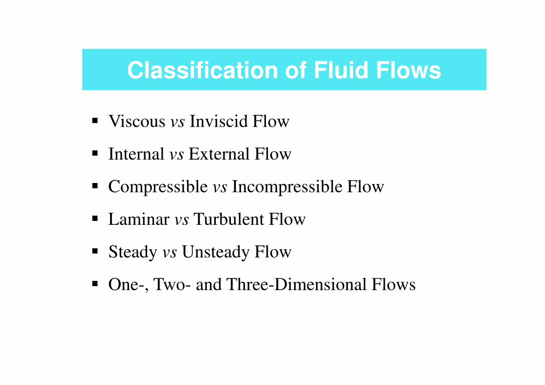
Classification of Fluid Flows
� Viscous vs Inviscid Flow
� Internal vs External Flow
� Compressible vs Incompressible Flow� Compressible vs Incompressible Flow
� Laminar vs Turbulent Flow
� Steady vs Unsteady Flow
� One-, Two- and Three-Dimensional Flows

The Reynolds number describes
the degree of turbulence.
The Reynolds number describes
the degree of turbulence.
uDRe =
ρ
Reynolds Number
forceviscous
forceinertia
Du
Du
]/[
]/[
Re
2
2
==
=
ρµ
µ
Turbulent fluids have viscosity, but we usually measure
viscosity in laminar flow.

Wat er Dye
St ream line f low ing dye
� Laminar Flow: “Streamline” flow.
� Fluid moves in a
straight line with the
applied force.
� Layers slide by with
Wat er Dye
Turbulent f lowQuickTime?and a
TIFF (Uncompressed) decompressorare needed to see this picture.
� Layers slide by with
no swirls.
� Turbulent Flow: “Disorderly” flow.
� Small packets of fluid
moving in all directions
and all angles to
normal line of flow.

Viscosity

Some fluids move slowly.
They have a high viscosity.
Syrup
pours
It is very viscous.
pours
slowly.

Some fluids move quickly.
They have a low viscosity.
Water
It is less viscous.
pours
quickly.

Viscosity
� A fluid’s thickness or resistance to flow is called its viscosity.
� A fluid is said to be more viscous if it does not flow as readily as another fluid. not flow as readily as another fluid.

� Gases are less viscous than liquids,
so they flow very easily through
pipes.
Gases vs Liquids
� The particle theory helps us to understand that this resistance is due to the stronger attraction among particles.
Why?
� Different substances are composed of different particles and this is why fluids can have different viscosities.

� Viscosity is a useful and important fluid property.
� Industries produce liquids, such as lubricants, with
special viscosities. If motor oil is not viscous enough,
it will not protect the engine parts from friction; if it is
too viscous, it will not flow to all parts of the engine
that need protection. [Viscosity causes fluid to adhere
Importance of Viscosity
that need protection. [Viscosity causes fluid to adhere
to a surface – known as no-slip condition]
� Salad dressing must be thin enough to pour out of a
bottle, yet thick enough to coat lettuce properly.
� It influences the power needed to move an airfoil
through the atmosphere.
� It accounts for the energy losses associated with the
transport of fluids in ducts, channels, and pipes.
� It plays a primary role in the generation of turbulence.

� An object moving
through or on a fluid
meets resistance.F
vx
Fluid Resistance
� Force causes the fluid
to move.
� The velocity is
proportional to the
force.
Fvx ∝

� The resistance tends to
keep the fluid in place.
� Law of inertia
yvx
F
Velocity Gradient
� The fluid moves most
near the object and least
farther away.
� This is a velocity gradient
or strain rate or rate of
deformation.
yvx ∝
y

� Newton combined these
two proportionalities.
� This is the law of viscosity.yvx
F
Law of Viscosity
� A is the area of the
solid sliding on the fluid
� The constant µ is the
dynamic viscosity and
depends on the type of
fluid. dy
du
y
vAF x
µτ
µ
=
=
y

Viscous Behavior of Various Materials
18
Newtonian fluid:
the shear stress of
the fluid is directly
proportional to the
velocity gradient.

� Inviscid flow: The flow in which viscous effects do not significantly influence the flow and are thus neglected.
Inviscid Flow vs Viscous Flow
� Viscous flow: The flow in which viscous effects are important and cannot be ignored.

� The primary class of flows, which can be modeled as inviscid flow, is
external flows.
� Any viscous effects that may exist are confined to a thin layer, called a
boundary layer which is attached to the boundary. The inviscid flow
outside the boundary layer in an external flow is called free stream.
� For many flows, the boundary layers are so thin that the can simply be
ignored when studying the gross features (e.g., lift and drag and locate
possible separation points) of a flow around a streamlined body (e.g.,
Inviscid Flow vs Viscous Flow
possible separation points) of a flow around a streamlined body (e.g.,
airfoil).
� Inviscid flow is also encountered in contractions inside piping systems
(viscous effects require substantial areas in order to be significant), in
short regions of internal flows (called inviscid core length) where
viscous effects are negligible, and wake in high-Reynolds-number flow
around bodies
� Viscous flows include the broad class of internal flows, such as flows in
pipes, conduits and open channels. In such flows, viscous effects cause
substantial “losses” and account for the huge amounts of energy that
must be used to transport oil and gas in pipelines.

� In the 19th century, two schools of thought existed on fluid
mechanics.
� Hydraulicians: looked at experimental data and attempted to
generalize them into useful design equations. Their equations were
generally empirical, without much theoretical content.
� Hydrodynamicists: started with 2D- and 3D- equations and tried to
The History of Potential Flow and Boundary Layer
21
� Hydrodynamicists: started with 2D- and 3D- equations and tried to
apply them to practical problems. They ignored the viscous-friction
and density change term by hypothesizing a perfect fluid with zero
viscosity and constant density, in order to calculate the complete
behavior of many kinds of flows. These mathematical solutions
agreed to very well with some observed behavior (except involving
no solid surfaces, and etc).
� “Hydrodynamicists calculate that which cannot be observed;
hydraulicians observe that which cannot be calculated.”

� In 1904 Ludwig Prandtl introduced a new concept, called the
boundary layer: if a fluid flows past the leading edge of a flat
surface, there will generate a velocity profile. Inside the boundary
layer, the effects of viscosity are too large to be ignored. Outside the
boundary layer, the laws of perfect-fluid flow should be satisfactory.
� The calculations were still very difficult, and so only approximate
mathematical solutions were possible.
The History of Potential Flow and Boundary Layer
22
mathematical solutions were possible.
� But, this idea clarified numerous unexplained phenomena and
provided a much better intellectual basis for discussing complicated
flows.
� So, it is clear that the ideas of perfect-fluid flow and boundary layer
are intimately tied together.
� We will consider perfect-fluid or inviscid flows in this chapter, and
boundary layer in chapters 3 and 4.

Deformation of a Fluid Elements
General deformation of fluid element is rather complex; however, we can
break the different types of deformation or motion into a superposition of
each type.
23
Velocity Angular Velocity
Linear Strain Rate Shear Strain Rate
In order for these deformation rates to be useful in the calculation of fluid
flows, they must be expressed in terms of velocity and derivatives of velocity.
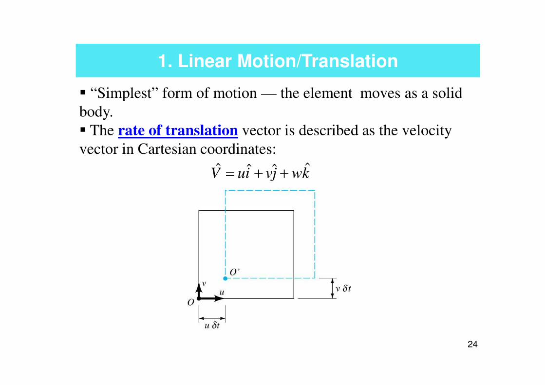
1. Linear Motion/Translation
� “Simplest” form of motion — the element moves as a solid
body.
� The rate of translation vector is described as the velocity
vector in Cartesian coordinates:
kwjviuV ˆˆˆˆ ++=
24
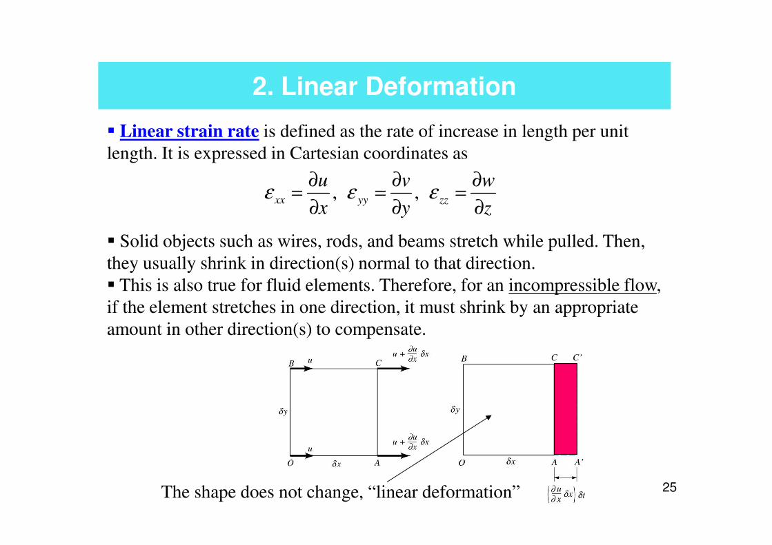
2. Linear Deformation
� Linear strain rate is defined as the rate of increase in length per unit
length. It is expressed in Cartesian coordinates as
� Solid objects such as wires, rods, and beams stretch while pulled. Then,
they usually shrink in direction(s) normal to that direction.
z
w
y
v
x
uzzyyxx
∂
∂=
∂
∂=
∂
∂= εεε ,,
25
they usually shrink in direction(s) normal to that direction.
� This is also true for fluid elements. Therefore, for an incompressible flow,
if the element stretches in one direction, it must shrink by an appropriate
amount in other direction(s) to compensate.
The shape does not change, “linear deformation”

2. Linear Deformation
Velocity gradients can cause deformation, “stretching” resulting in a change
in volume of the fluid element.
Rate of Change for one direction:
For all THREE directions: The volumetric strain rate is
26
For all THREE directions:
Vz
w
y
v
x
u
dt
dzzyyxx
ˆ)(1⋅∇=
∂
∂+
∂
∂+
∂
∂=++=
∀
∀εεε
δ
δ
� The rate of increase of volume of a fluid element per unit volume is
called as volumetric strain rate or volumetric dilatation rate or bulk
strain rate. It is positive if the volume increases.
�The linear deformation is zero for incompressible fluids. 0ˆ =⋅∇ V
The volumetric strain rate is
the sum of the linear strain
rates in three mutually
orthogonal directions.

3. Angular Motion/Rotation
� Angular velocity or rate of rotation at a point is defined as the average
rotation rate of two initially perpendicular lines that intersect at that point:
Angular motion results from
cross derivatives.
27

3. Angular Motion/Rotation
The rotation of the element about the z-axis is the average of the angular
velocities :
Likewise, about the y-axis, and the x-axis:
Counterclockwise rotation is considered positive
and
28
and
The three components gives the rotation vector:
Using vector identities, the rotation vector is one-half the curl of the
velocity vector:
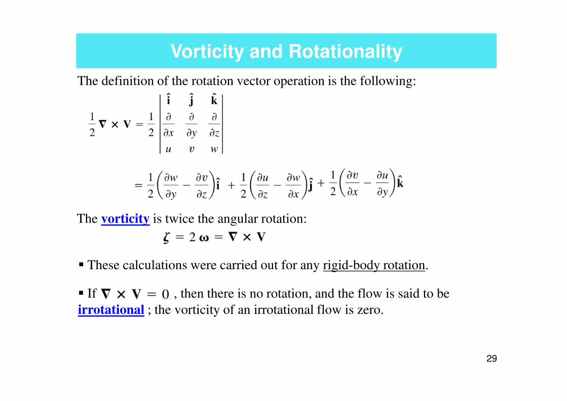
Vorticity and Rotationality
The definition of the rotation vector operation is the following:
29
� If , then there is no rotation, and the flow is said to be
irrotational ; the vorticity of an irrotational flow is zero.
The vorticity is twice the angular rotation:
� These calculations were carried out for any rigid-body rotation.

Vorticity and Rotationality
For a flow to be irrotational, each of the rotation (and therefore vorticity)
vector components must be equal to zero.
The z-component:
The x-component lead to a similar result:
30
The y-component lead to a similar result:

Vorticity and Rotationality
� The vorticity vector in cylindrical coordinates (r, θ, z):
� For 2-D flow in the rθ-plane:
zrzr
rz e
u
r
ru
re
r
u
z
ue
z
uu
rˆ
)(1ˆˆ
1ˆ
∂
∂−
∂
∂+
∂
∂−
∂
∂+
∂
∂−
∂
∂=
θθζ θ
θθ
31
� For 2-D flow in the rθ-plane:
zr e
u
r
ru
rˆ
)(1ˆ
∂
∂−
∂
∂=
θζ θ

Example
Example: A velocity field in a particular flow is given by V = 20y2i – 20xyj
m/s. Calculate the angular velocity and the vorticity vector at the point (1,
-1, 2).
32

Example
Example: Determine whether the following 2-D flows are rotational or
irrotational:
(a) u = -2y, v = 3x;
(b) v = 0, w = 3yz;
(c) u = 2x, w = 2z.
33

The Irrotational Flow Approximation
� Irrotational approximation:
� We must keep in mind that the assumption of irrotationality
is an approximation, which may be appropriate in some
regions of a flow field, but not in other regions.
� In general, inviscid regions of flow far away from solid walls
0ˆˆ ≈×∇= Vζ
34
� In general, inviscid regions of flow far away from solid walls
and wakes of bodies are also irrotational.
� However, there are situations in which an inviscid region of
flow may not be irrotational (e.g., solid-body rotation).

Inviscid Flow: Irrotational Flow
Examples where inviscid flow theory can be used:
35
Viscous Region - RotationalInviscid Region – Irrotational

4. Angular Deformation/Shear Strain
� Shear strain rate at a point is defined as half of the rate of
decrease of the angle between two initially perpendicular lines that
intersect at that point.
� Consider a fluid element translating and deforming in 2-D xy-
plane, the shear strain rate, initially perpendicular lines in the x- and
y-directions: ∂∂ vud 11
36
� Consider 3-D, the shear strain rate in Cartesian coordinates:
∂
∂+
∂
∂=−=
x
v
y
u
dt
dxy
2
1
2
1αε
∂
∂+
∂
∂=
∂
∂+
∂
∂=
∂
∂+
∂
∂=
x
w
z
v
z
u
x
w
x
v
y
uyzzxxy
2
1
2
1
2
1εεε
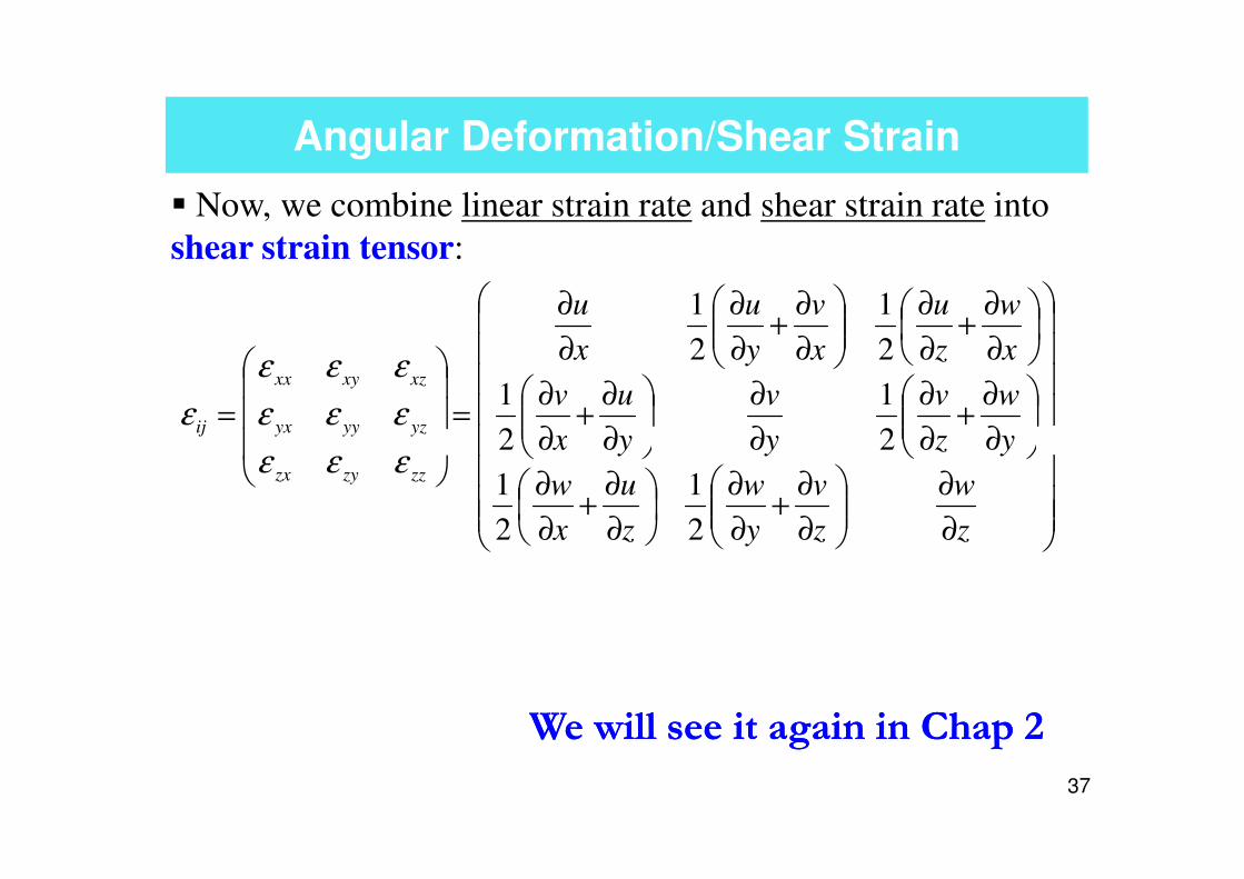
Angular Deformation/Shear Strain
� Now, we combine linear strain rate and shear strain rate into
shear strain tensor:
∂
∂+
∂
∂
∂
∂
∂
∂+
∂
∂
∂
∂+
∂
∂
∂
∂+
∂
∂
∂
∂
=
=y
w
z
v
y
v
y
u
x
v
x
w
z
u
x
v
y
u
x
u
yzyyyx
xzxyxx
ij2
1
2
1
2
1
2
1
εεε
εεε
ε
37
∂
∂
∂
∂+
∂
∂
∂
∂+
∂
∂
∂∂∂
∂∂
z
w
z
v
y
w
z
u
x
w
yzyyxzzzyzx
2
1
2
1
22εεε
We will see it again in Chap 2We will see it again in Chap 2

Example
Example: A velocity field in a particular flow is given by V = 20y2i – 20xyj
m/s. Calculate the nonzero strain rate components at the point (1, -1, 2).
38

Conservation of Mass: Cartesian Coordinates
The differential form of the equation for Conservation of Mass:
In vector notation, the equation is the following:
If the flow is steady and compressible:
39
The Continuity Equation
If the flow is steady and compressible:
If the flow is steady and incompressible:

Examples
Example: Assuming ρ to be constant, do the following flows satisfy continuity?
(a) u = -2y, v = 3x;
(b) u = 0, v = 3xy;
40

Streamlines
� A streamline is a line drawn
through the flow field in such a
manner that the local velocity vector
is tangent to the streamline at every
point along the line at that instant.
� The tangent of the streamline at a
41
� The tangent of the streamline at a
given time gives the direction of the
velocity vector. A streamline does
not indicate the magnitude of the
velocity.
� The flow pattern shown by the
streamlines is an instantaneous
visualization of the flow field.

Conservation of Mass: Cylindrical Coordinates
42
If the flow is steady and compressible:
If the flow is steady and incompressible:
The Continuity Equation

Examples
Example: Check the following incompressible flows for continuity and
determine the vorticity of each:
(a) vθ = 6r, vr = 0;
(b) vθ = 0, vr = -5/r.
43

Stream Functions
Stream Functions are defined for steady, incompressible, 2D flow.
2-D Continuity Equation:
Then, we define the stream functions as follows:
44
Now, substitute the stream function into the continuity equation:
Any flow that satisfies stream
function automatically satisfies
the continuity condition.

Stream Functions
The slope at any point along a streamline:
Streamlines have constant ψ, thus dψ = 0:
45
Streamlines have constant ψ, thus dψ = 0:
w
dz
v
dy
u
dx==
The stream function is
constant along a streamline.
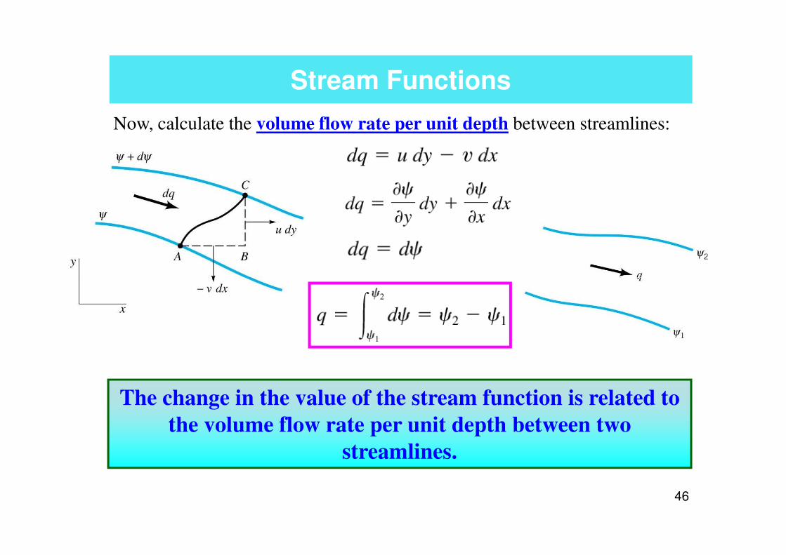
Stream Functions
Now, calculate the volume flow rate per unit depth between streamlines:
46
The change in the value of the stream function is related to
the volume flow rate per unit depth between two
streamlines.

� Incompressible, planar stream function in cylindrical coordinates:
� Incompressible, axisymmetric stream function in cylindrical
coordinates:
Stream Functions in Cylindrical Coordinates
47
coordinates:
0)()(1
=∂
∂+
∂
∂
z
u
r
ru
r
zr
rru
zru zr
∂
∂=
∂
∂−=
ψψ 11

Interpretation of Stream Function
� A single variable (ψ) replaces two variables (u and v); once ψ
is known, both u and v can be generated.
� The stream function satisfies the continuity equation.
� Curves of constant ψ are streamlines of the flow.
� The difference in the value of ψ from one streamline to
48
� The difference in the value of ψ from one streamline to
another is equal to the volume flow rate per unit width
between the two streamlines.
� In steady flow, there is no flow across (perpendicular) to a
streamline.
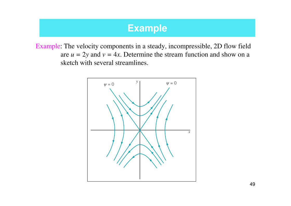
Example
Example: The velocity components in a steady, incompressible, 2D flow field
are u = 2y and v = 4x. Determine the stream function and show on a
sketch with several streamlines.
49
Streamlines
� For real fluid flows, the fluid adjacent to the boundary of a solid body
does not move relative to body – it sticks to the wall. So, in real fluids
the wall is a streamline of zero velocity.
� But, the perfect fluid has no tendency to stick to walls because it has
no viscosity. So, the streamline adjacent to a solid body in perfect-fluid
flow is one with finite velocity.
� This leads to the idea that we may divide a perfect-fluid flow along a
50
� This leads to the idea that we may divide a perfect-fluid flow along a
streamline and substitute a solid body for the flow on one side of the
streamline.

Potential Flow
� In the region outside the boundary layer, where the fluid may be
assumed to have no viscosity, the mathematical solution takes on the
form known as irrotational flow (also known as potential flow).
� This form is analogous to the flow of heat in a temperature field or to
the flow of charge in an electrostatic field. All these flows obey
Laplace’s equation under certain restrictions (for example: steady-state
mass balance for a constant-density fluid).
51
mass balance for a constant-density fluid).
� Not every velocity potential satisfies Laplace’s equation, and so not
every velocity potential represents a potential flow. For example, φ = x2,
x2 + y2, ex, sin x do not satisfy Laplace’s equation, so they cannot
represent potential flows because they violate the mass balance for a
constant-density fluid.

Consider a velocity field that is given by the gradient of a scalar function φ(called velocity potential function):
Such velocity field is called a potential flow (or an irrotational flow) and
possesses the property that the vorticity ω, which is the curl of a velocity
vector, is zero:
Potential Flow: Velocity Potential
φ∇=V̂
52
vector, is zero:
With the velocity given by the gradient of a scalar function, the differential
continuity equation ( ), for an incompressible flow, gives
which is known as Laplace’s equation.
0ˆ =×∇= Vω
02 =∇=∇⋅∇ φφ
The flow must be irrotational if there is a velocity potential.
0ˆ =⋅∇ V

Potential Flow: Velocity Potential
For irrotational flow, there exists a velocity potential:
Take one component of vorticity to show that the velocity potential is irrotational:
53
Substitute u and v components of velocity potential:
02
1 22
=
∂∂
∂−
∂∂
∂
xyyx
φφWe could do this to show all vorticity components are zero.
The flow must be irrotational if there is a velocity potential.

If the curl of a vector is zero, the vector can be expressed as the gradient of
a velocity potential.
Potential Flow: Velocity Potential
Then, rewriting the u, v, and w components as a vector:
For irrotational, planar flow:
Now substitute the stream function:
54
Then for incompressible irrotational flow:
Now substitute the stream function:
Then, Laplace’s Equation
Pierre Laplace (1749-1827)

Potential Flow: Velocity Potential
� Potential flows are
irrotational – vorticity is
zero.
� If the vorticity is present
(e.g., boundary layer, wake),
then the flow cannot be
55
then the flow cannot be
described by Laplace’s
equation.

Potential Flow: Velocity Potential
Laplacian Operator in Cartesian coordinates:
Laplacian Operator in cylindrical coordinates:
If a Potential Flow exists,
with appropriate boundary
conditions, the entire velocity
and pressure field can be
specified.
56
where the gradient in cylindrical coordinates, the gradient operator,
Then,
May choose cylindrical
coordinates based on the
geometry of the flow problem,
i.e., pipe flow.

Potential Flow: Velocity Potential
Lines of constant ψ are streamlines:
Now, the change of φ from one point (x, y) to a nearby point (x + dx, y + dy):
57
Along lines of constant φ, we have dφ = 0,
0
The equipotential lines are orthogonal to streamlines where they intersect.
Lines of constant φ are called equipotential lines.
Potential Flow: Velocity Potential
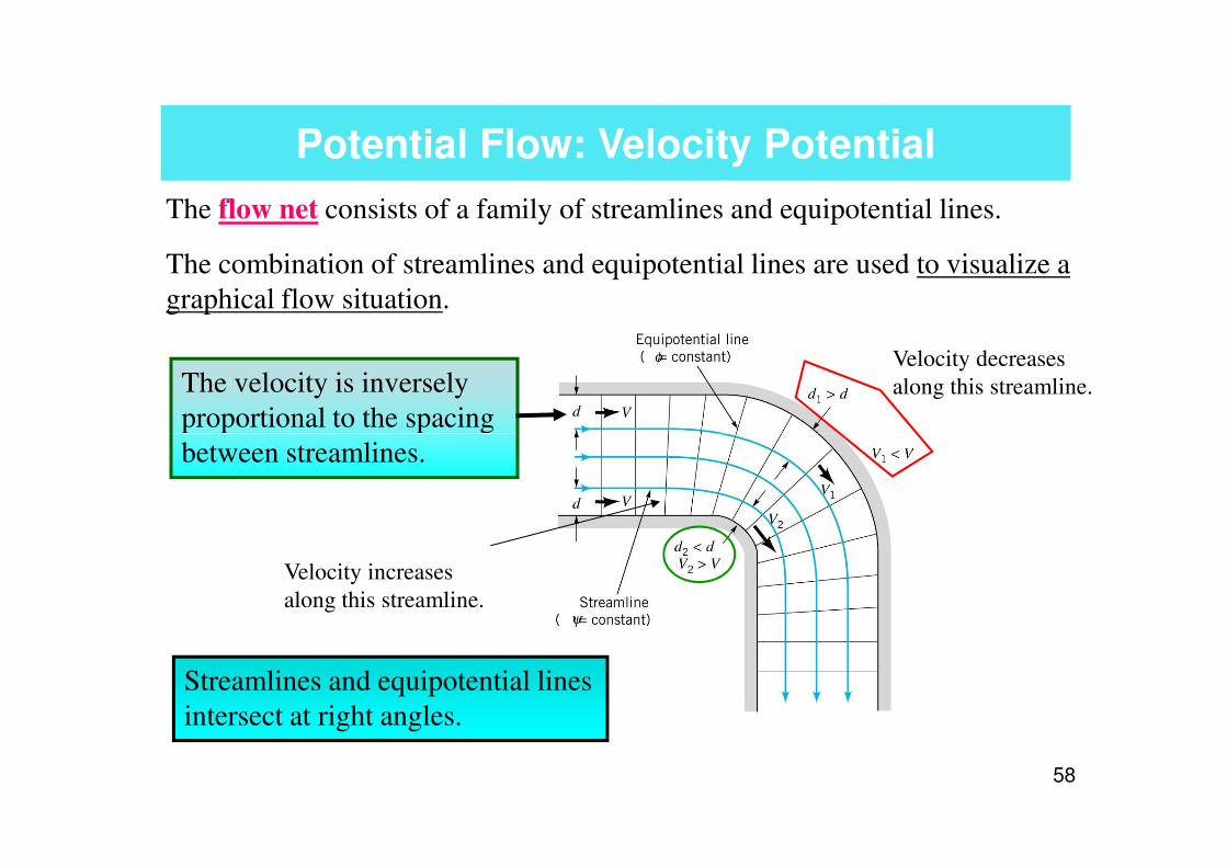
The flow net consists of a family of streamlines and equipotential lines.
The combination of streamlines and equipotential lines are used to visualize a
graphical flow situation.
The velocity is inversely
proportional to the spacing
Velocity decreases
along this streamline.
58
between streamlines.
Velocity increases
along this streamline.
Streamlines and equipotential lines
intersect at right angles.

Stream Function and Velocity Potential
� The stream function is
defined by continuity; the
Laplace equation for ψresults from irrotationality.
59
� The velocity potential is
defined by irrotationality;
the Laplace equation for φresults from continuity. 0
2
1 22
=
∂∂
∂−
∂∂
∂
xyyx
φφ

Potential Flow: Plane Potential Flows
Velocity components for steady, incompressible, irrotational, 2D regions of
flow in terms of velocity potential and stream function in various
coordinate systems:
Planar, Cartesian:
Planar, Cylindrical:
60
Planar, Cylindrical:
Planar, Cartesian:
Planar, Cylindrical:
rru
zru zr
∂
∂=
∂
∂−=
ψψ 11
Axisymmetric, Cylindrical:
Axisymmetric, Cylindrical:
zu
ru zr
∂
∂=
∂
∂=
φφ

The Conversion between Velocity Field, Stream Function and Velocity Potential
φψ ⇔⇔ ),( vu
61
φ⇔),,( wvu

Incompressible? Continuity equation? Stream function exists? Irrotational? Velocity
potential exists?
Incompressible? Satisfy
continuity equation?
Stream function
Irrotational? Velocity
potential exists?
62
exists?
0=•∇ V
02 =∇ φ 02 =∇ ψ
0or0 == ζω

Example
Example: A velocity potential in 2D flow is . Find the stream
function for this flow.
22yxy −+=φ
63

Example
Example: The 2D stream function for a flow is . Find
the velocity potential for this flow.
xyyx 7469 +−+=ψ
64

Example
Example: In a 2D incompressible flow, the fluid velocity components are
given by and . Show that the flow satisfied the
continuity equation and obtain the expression for the stream function.
If the flow is potential, obtain also the expression for the velocity
potential.
yxu 4−= xyv 4−−=
65

Example
Example: The 2D flow of a non-viscous, incompressible fluid in the vicinity of
the 90º corner is described by the stream function .
Determine the corresponding velocity potential. θψ 2sin2 2
r=
66α
πθφ απ cos/
Ar=
α
πθψ απ sin/
Ar=

� Before we discuss the elemental flows, let’s visit this
website:
http://simscience.org/fluid/green/potential.html
Elementary Flows
67
� Next we will learn how the velocity fields of some
elementary and complex flows can be expressed in
terms of stream function and velocity potential.
http://simscience.org/fluid/green/potential.html

1. Uniform Flow
Question: Do φ1 = Ax and φ2 = Ax + By satisfy Laplace’s equation?
For φ1 = Ax , u = ∂φ1/∂x = A, v = ∂φ1/∂y = 0
So, φ1 describes a uniform, steady flow of velocity A in the positive x
direction. This might be the description of a wind blowing over the ocean at
a steady, uniform velocity of A.
68
a steady, uniform velocity of A.
For φ2 = Ax + By, u = ∂φ2/∂x = A, v = ∂φ2/∂y = B
So, φ2 describes a uniform, constant-velocity flow with velocity (A2 + B2)1/2,
making the angle arctan (B/A) with the x axis.
These uniform flows are not of much practical interest
alone, but they can be combined with other flows to solve
more interesting problems.

1. Uniform Flow
For Uniform Flow in an arbitrary direction, α:
φ = Ux
ψ = Uy
u = U
v= 0
69

2. Source and Sink Flow
0
Now, obtain the stream function for the flow:
Integrating to obtain the solution: rm
ln2ππππ
φφφφ =
( ) mvr r =π2
vr vθ
70
The streamlines are radial lines and the equipotential
lines are concentric circles centered about the origin:
φ lines
ψ lines

2. Source and Sink Flow
� If m is positive, the flow is source; if m is negative, the flow is
sink.
is the volume rate of flow per unit depth issuing from the
source or sink, where Q is flow rate, and L is height.
� These flows are of practical significance in the petroleum
LQm /=
71
industry; it describes the flow into oil well in a thick horizontal
stratum.
� The equations vr = m/2πr, vθ = 0 show that the radial flow
velocity becomes infinite at r = 0 (mathematical singularity); thus,
this equation cannot describe any real flow at r = 0.

Examples
Example: A nonviscous, incompressible fluid flows between wedge-shaped
walls into a small opening. The velocity potential (in m2/s), which
approximately describes this flow is φ = -2 ln r. Determine the
volume rate of flow (per unit length) into the opening.
72

3. Vortex Flow
In vortex flow the streamlines are concentric circles, and the equipotential
lines are radial lines.
where K is a constant, namely the strength of the vortex.
Solution:
The sign of K determines whether the flow rotates
clockwise (-) or counterclockwise (+).
73
clockwise (-) or counterclockwise (+).
In this case, ,
The tangential velocity varies inversely with
the distance from the origin.
At the origin it encounters a singularity
becoming infinite.
φ lines
ψ lines

3. Vortex Flow
� Rotation refers to the orientation of a fluid element and not the path
followed by the element. The elements deform to maintain a constant
orientation.
� In general flow there is both deformation and rotation.
�An ideal flow is one that has no viscosity and is incompressible.
74
� If an ideal flow is initially irrotational, it will remain irrotational.
� Two vortices: free vortex and forced vortex.
� The swirling motion of the water as it drains from a bathtub is similar to
that of a free vortex, while the motion of a liquid contained in a tank is
rotated about its axis with angular velocity corresponds to a forced vortex.

Free Vortex and Forced Vortex
Irrotational Flow: Free Vortex Rotational Flow: Forced Vortex
Traveling from A to B, consider two sticks
Velocity
increases
inward.
Velocity
increases
outward.
i.e., water
draining from a
bathtub
i.e., a rotating tank
filled with fluid
75
Initially, sticks aligned, one in the flow direction,
and the other perpendicular to the flow.
As they move from A to B the perpendicular-
aligned stick rotates clockwise, while the flow-
aligned stick rotates counter clockwise.
The average angular velocities cancel each other,
thus, the flow is irrotational.
Irrotational Flow: Rotational Flow: Rigid Body Rotation
Initially, sticks aligned, one in the
flow direction, and the other
perpendicular to the flow.
As they move from A to B the sticks
move in a rigid body motion, and thus
the flow is rotational.
0ˆˆ =×∇= Vζζζζ V̂2ˆ ×∇== ωζ

Free Vortex and Forced Vortex
76

A simple analogy can be made
between flow A and a merry-go-
round or roundabout, and flow B
and a Ferris wheel.
As children revolve around a
roundabout, they also rotate at
the same angular velocity as that
of the ride itself. This is analogous
to a rotational flow.
In contrast, children on a Ferris
wheel always remain oriented in
77
A simple analogy: (a) rotational
circular flow is analogous to a
roundabout, while (b) irrotational
circular flow is analogous to a
Ferris wheel.
wheel always remain oriented in
an upright position as they trace
out their circular path. This is
analogous to an irrotational flow.

Tornadoes and Hurricanes
� A combined vortex flow is one in which there is a forced vortex at the core, and a free
vortex outside the core.
� The minimum pressure at the vortex center can give rise to a “secondary flow” which
is produced by the pressure gradient in the primary (vortex) flow.
� In the region near the ground, the wind velocity is decreased due to the friction
provided by the ground.
� However, the pressure difference in the radial direction causes a radially inward flow
adjacent to the ground, and upward flow at the vortex center.
78
Pressure difference between the vortex
center and outer edge:
p1 – p0 = –ρVmax2

Circulation
� Circulation (Γ) or vortex strength gives a measure of the average of
rate of rotation of fluid particles that are situated in an area that is bounded
by a closed curved.
� This concept is often useful when evaluating forces (such lift force)
developed on bodies immersed in moving fluids.
� It is defined as the line integral of the tangential component of the
velocity (V) around a closed curve fixed in the flow.
79
velocity (V) around a closed curve fixed in the flow.
� ΓΓΓΓ = 0 for irrotational flow.
� If there are singularities enclosed within the curve, Γ ≠ 0, for example:
free vortex.

Circulation: Free Vortex
For the free vortex:
(Integrate the entire circle)
Γ= 0
80
The circulation is non-zero and constant for the free vortex:
The velocity potential and the stream function for the free vortex can
be rewritten in terms of the circulation:

Examples
Example: The pressure far from an irrotational vortex (a simplified tornado) in
the atmosphere is zero gauge. If the velocity at r = 20 m is 20 m/s, estimate
the velocity and the pressure at r = 2 m.
81

Circulation
How is circulation calculated from rpm and radius?
82

Example
Example: A liquid drains from a large tank through a small opening. A vortex
forms whose velocity distribution away from the tank opening can be
approximated as that of a free vortex having a velocity potential
Determine an expression relating the surface shape to the strength of
the vortex as specified by the circulation.
θπφ )2/(Γ=
83

4. Doublet Flow
Combination of an equal Source and Sink pair.
Rearrange and take tangent,
84
Note, the following:
Substituting the above expressions,
and
Then,
If a is small, then tangent of angle is approximated by the angle:

4. Doublet Flow
Now, we obtain the doublet flow by letting the source and sink approach one
another (a→ 0), and letting the strength increase (m→∞).
85
K is the strength of the doublet, and is equal
to ma/π.
is then constant.
The corresponding velocity potential then is the following:
Streamlines of a Doublet:ψ lines Doublet strength is for a
double oriented in the
negative x-direction.

Summary of Basic Flows
u = U
v = 0
Γ = 0
Γ = 0
86
Γ = 0Origin is singular point
Origin is singular point
Γ = K around any closed curved enclosing origin
Γ = 0 around any closed curved NOT enclosing origin
Origin is singular point Γ = around any closed curved

Superposition of Basic Flows
� Because potential flows are governed by linear partial differential
equations, the solutions can be combined in superposition; we will
superimpose simple functions to create flows of interest.
� If φ1 and φ2 are each solutions of the Laplace equation, then Aφ1, (A +
φ1), (φ1 + φ2), and (Aφ1 + φ2) are also solutions,.
� Thus, some of the basic ψ and φ can be combined to yield a streamline
87
� Thus, some of the basic ψ and φ can be combined to yield a streamline
that represents a particular body shape, or complicated incompressible,
plane flow.
� The superposition representing a body can lead to describing the flow
around the body in detail.
� The superposition is only valid for irrotatioanal flow fields for which the
equations for φ and ψ are linear.
� The velocity at any point in the composite field is the vector sum of the
velocities of the individual flow fields.

1. Rankine Half-Body
The Rankine Half-Body is a combination of a source and a uniform flow.
88
Stream Function (cylindrical coordinates):
Velocity Potential (cylindrical coordinates):

1. Rankine Half-Body
There will be a stagnation point, somewhere along the negative x-axis where
the velocities due to the source and uniform flow are cancelled (θ = π).
For the source: For the uniform flow: θcosUvr =
For θ = π, Uv r =
Then, for a stagnation point, at some x = -b (r = b), θ = π:
m
89
r
mUvr
π2== and
Now, the stagnation streamline can be defined by evaluating y at r = b, and
θ = π . The value of ψ at the stagnation point:
θπ
θψ2
sinm
Ur +=

1. Rankine Half-Body
Since m/2 = πbU, it follows that the equation of the streamline passing
through the stagnation point, and gives the outline of the Rankine half-
body:
Then,
For inviscid flow, a streamline can be replaced by a solid boundary. So,
90
For inviscid flow, a streamline can be replaced by a solid boundary. So,
the source and uniform can be used to describe the flow around a
streamlined body placed in a uniform stream – half-body.
The other streamlines can be obtained by setting ψ = constant.
Singularity (inside the body)

1. Rankine Half-Body
The width of the half-body:Total width = 2ππππb
The magnitude of the velocity (V) at any point in the flow:
and
( )r
b θπθ
−=sin
91
Noting,
Knowing the velocity we can now determine the pressure field using the
Bernoulli Equation:
po and U are at a point far away from the body and are known.
1. Rankine Half-Body
� We wish to find the flow pattern around some arbitrary body.
This is normally done by combining uniform flows, sources,
sinks, etc.
� When a combination is found that produces a streamline with
the shape of the body in question, the flow outside the
streamline is a representation of the flow around the body.
92
streamline is a representation of the flow around the body.
� The flow inside that line normally has no meaning and is
ignored.
� The singularity in the flow field (source) only occurs inside
the body.

1. Rankine Half-Body
� The velocity tangent to the surface of the body is not zero,
i.e., the fluid “slips” by the boundary (as neglecting viscosity).
So, all potential flows differ from the flow of real fluids
(considering viscosity) and do not accurately represent the
velocity very near the boundary. However, outside this layer,
the velocity distribution will generally correspond to that
93
the velocity distribution will generally correspond to that
predicted by potential flow theory if flow separation does not
occur.
� The pressure distribution along the surface will closely
approximate that predicted from the potential flow theory since
the boundary layer is thin, and there is little variation of
pressure through the boundary layer.

Example
Example: The shape of a hill arising from a plain can be approximated with the top
section of a half-body. The height of the hill approaches 60 m.
(a) When a 60 km/hr wind blows toward the hill, what is the magnitude
of the air velocity at a point on the hill directly above the origin (point 2)?
(b) What is the elevation of point (2) above the plain and what is the
difference in pressure between point (1) on the plain far from the hill and
point (2)? Assume an air density of 1.23 kg/m3.
94
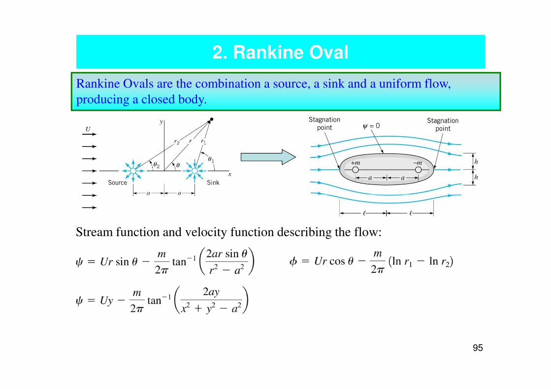
2. Rankine Oval
Rankine Ovals are the combination a source, a sink and a uniform flow,
producing a closed body.
95
Stream function and velocity function describing the flow:

2. Rankine Oval
The streamline ψ = 0 forms the surface of a body of length 2l and width 2 h
placed in a uniform flow.
Ua/m is large � slender body
Ua/m is small � blunt shape body
96
The body half-length
The body half-width
“Iterative”
2/1
1
+=
Ua
m
a
l
π
−
=
a
h
m
Ua
a
h
a
h π2tan1
2
12

2. Rankine Oval
Ua/m is large � slender body
Ua/m is small � blunt shape body
97
Ua/m is small � blunt shape body
2. Rankine Oval
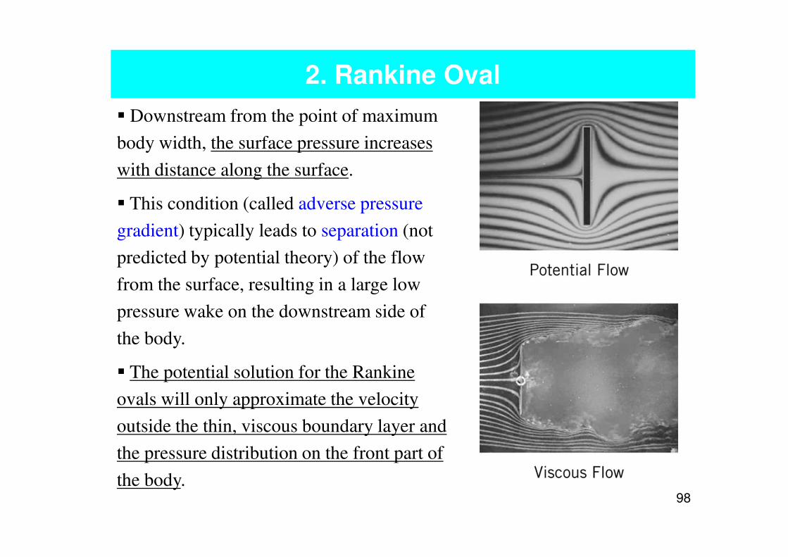
� Downstream from the point of maximum
body width, the surface pressure increases
with distance along the surface.
� This condition (called adverse pressure
gradient) typically leads to separation (not
predicted by potential theory) of the flow
from the surface, resulting in a large low
98
from the surface, resulting in a large low
pressure wake on the downstream side of
the body.
� The potential solution for the Rankine
ovals will only approximate the velocity
outside the thin, viscous boundary layer and
the pressure distribution on the front part of
the body.

3.1. Flow Around a Stationary Circular Cylinder
Combines a uniform flow and a doublet flow
and
For the ψ to represent flow around a cylinder, ψ = constant for r = a (a = the
radius of the circular cylinder):
K = Ua2
99
K = Ua2
Then, and
Then the velocity components:
Doublet strength

3.1. Flow Around a Stationary Circular Cylinder
On the surface of the cylinder (r = a):
The maximum velocity occurs at the top and bottom of the cylinder,
magnitude of 2U (θ = ± π/2).
vrs = 0
The figure shows the pattern
of streamlines for this flow.
Why are the
streamlines so
close here?
100
of streamlines for this flow.
We disregard the doublet flow
on the inside of the circle r = a
and imagine that a solid
cylinder replaces this portion
of the flow. A remarkable
feature is the symmetry of the
flow upstream and
downstream of the cylinder.
Why are the streamlines so far here?
close here?
No slip or slip?

3.1. Flow Around a Stationary Circular Cylinder
Pressure distribution on a circular cylinder found with the Bernoulli equation
Then substituting for the surface velocity:
101
Theoretical and experimental agree well
on the front portion of the cylinder. The
actual surface pressures and ideal values
agree for a distance up to β = 60°.
Flow separation on the back-half in the
real flow due to viscous effects causes
differences between the theory and
experiment. So, the ideal flow is no
longer valid.
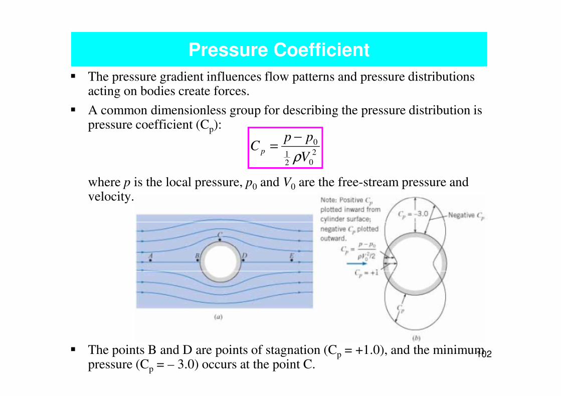
� The pressure gradient influences flow patterns and pressure distributions acting on bodies create forces.
� A common dimensionless group for describing the pressure distribution is pressure coefficient (Cp):
where p is the local pressure, p0 and V0 are the free-stream pressure and velocity.
Pressure Coefficient
2
021
0
V
ppC p
ρ
−=
102
velocity.
� The points B and D are points of stagnation (Cp = +1.0), and the minimum pressure (Cp = – 3.0) occurs at the point C.

3.1. Flow Around a Stationary Circular Cylinder
Inviscid flow past a circular
cylinder:
(a) streamlines for the flow if
there were no viscous effects.
103
(b) pressure distribution on
the cylinder’s surface,
(c) free-stream velocity on
the cylinder’s surface.
The pressure distribution up to the
point of separation is very nearly
the same as that predicted by
potential flow.

Boundary layer
characteristics on a circular
cylinder:
(a) boundary layer
separation location.
3.1. Flow Around a Stationary Circular Cylinder
Wake
104
(b) typical boundary layer
velocity profiles at various
locations on the cylinder,
(c) surface pressure
distributions for inviscid
flow and boundary layer
flow.
Turbulent or laminar data
matches better with
irrotational flow
approximation? Why?

� From Euler’s equation for pressure gradient and acceleration along a
pathline,
� The fluid particle accelerates (at > 0) if the pressure decreases with
distance along a pathline (∂p/�s < 0) – favorable pressure gradient.
Favorable and Adverse Pressure Gradient
s
pat
∂
∂−=ρ
105
� The fluid particle decelerates (at < 0) if the pressure increases with
distance along a pathline (∂p/�s > 0) – adverse pressure gradient.

� Flow separation occurs when the fluid pathlines adjacent to body deviates
from the contour of the body and produce a wake.
� It tends to increase drag, reduce lift and produce unsteady forces leading
to structural failure (e.g., Tavoma Narrows Bridge in 1904).
� The prediction and control of separation is continuing challenge for
engineers involved with the design of fluid systems.
Flow Separation
106

3.1. Flow Around a Stationary Circular Cylinder
The resultant force per unit length acting on the cylinder can be determined
by integrating the pressure over the surface (equate to lift and drag).
(Drag)
(Lift)
107
Substituting
Evaluating the integrals:
Both drag and lift are predicted to be zero on fixed cylinder in a uniform
flow. The zero-life prediction is acceptable for a real flow, but the zero-
drag result is unacceptable.
Jean le Rond
d’Alembert
(1717-1783)

3.1. Flow Around a Stationary Circular Cylinder
� Mathematically, this makes sense since the pressure distribution is
symmetric about cylinder (because of the symmetric pressure distribution, the
force on the front half cancels that one the rear half to produce zero drag).
� However, in practice/experiment, we see substantial drag on a circular
cylinder (and called as d’Alembert’s Paradox, 1717-1783).
Potential theory incorrectly predicts that the drag on a cylinder is zero.
108
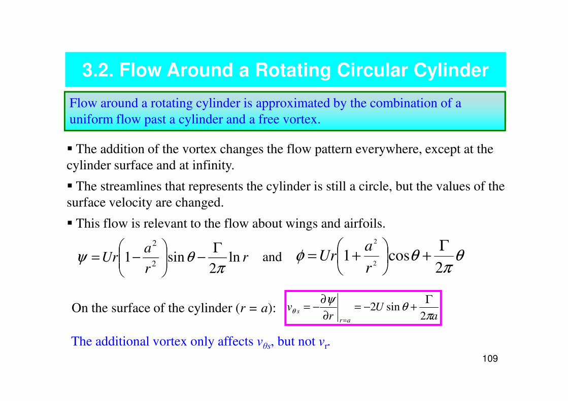
3.2. Flow Around a Rotating Circular Cylinder
� The addition of the vortex changes the flow pattern everywhere, except at the
cylinder surface and at infinity.
� The streamlines that represents the cylinder is still a circle, but the values of the
surface velocity are changed.
Flow around a rotating cylinder is approximated by the combination of a
uniform flow past a cylinder and a free vortex.
109
surface velocity are changed.
� This flow is relevant to the flow about wings and airfoils.
rr
aUr ln
2sin1
2
2
πθψ
Γ−
−= θ
πθφ
2cos1
2
2 Γ+
+=
r
aUrand
aU
rv
ar
sπ
θψ
θ2
sin2Γ
+−=∂
∂−=
=
On the surface of the cylinder (r = a):
The additional vortex only affects vθs, but not vr.

3.2. Flow Around a Rotating Circular Cylinder
� If Γ = 0, then θstag = 0 or π,
i.e., the stagnation points occur at
the front and rear of the cylinder.
� If -1 ≤ Γ/(4πUa) ≤1, then the
stagnation points occur at some
Uastag
πθ
4sin
Γ=The stagnation points occur at θ = θStag where (vθ = 0):
110
stagnation points occur at some
other location on the surface as
Figures (b) and (c).
� If ||||Γ/(4πUa)|||| > 1, then the
stagnation point is located away
from the cylinder. There is a
portion of fluid that is trapped
next to the surface and continually
rotates around the cylinder.
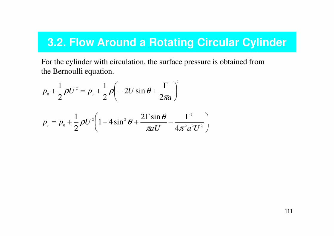
3.2. Flow Around a Rotating Circular Cylinder
For the cylinder with circulation, the surface pressure is obtained from
the Bernoulli equation.
2
2
0
2sin2
2
1
2
1
Γ+−+=+
aUpUp
s
πθρρ
Γ
−Γ
+−+=2
22 sin2sin41
1Upp
θθρ
111
Γ−
Γ+−+=
222
22
0
4
sin2sin41
2
1
UaaUUpp
s
ππ
θθρ

3.2. Flow Around a Rotating Circular Cylinder
112

3.2. Flow Around a Rotating Circular Cylinder
0=x
F
Substituting this equation into Fy, for the lift, and integrated, yields
For the rotating cylinder, no force in the direction of the uniform flow is developed.
Substituting this equation into Fx, for the drag, and integrated, yields
Γ−= UFy
ρ
Magnus Effect Magnus Effect Magnus Effect Magnus Effect ––––
Lift on rotating bodiesLift on rotating bodiesLift on rotating bodiesLift on rotating bodies
113
The negative sign means that if U is positive in the positive x direction, and
circulation is positive (a free vortex with counterclockwise rotation), the
direction is downward.
Potential flow past a cylinder with circulation gives zero drag, but non-zero lift.
Lift on rotating bodiesLift on rotating bodiesLift on rotating bodiesLift on rotating bodies
http://www.grc.nasa.gov/WWW/K-12/airplane/cyl.html
The equation relating lift force on airfoils to ρ, U, and Γ is called Kutta-
Joukowski law.
3.2. Flow Around a Rotating Circular Cylinder
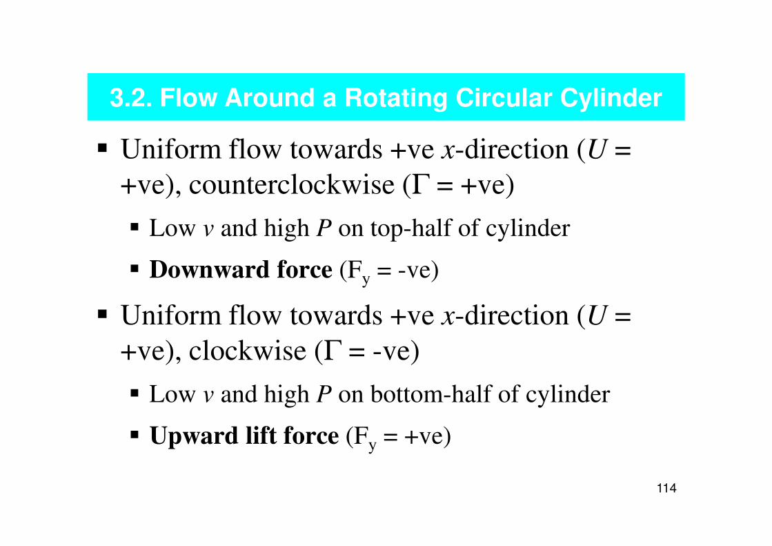
� Uniform flow towards +ve x-direction (U =
+ve), counterclockwise (Γ = +ve)
� Low v and high P on top-half of cylinder
� Downward force (Fy = -ve)
114
� Downward force (Fy = -ve)
� Uniform flow towards +ve x-direction (U =
+ve), clockwise (Γ = -ve)
� Low v and high P on bottom-half of cylinder
� Upward lift force (Fy = +ve)


