3/14/2011

1

Digital Image Processing

Filtering in the Frequency Domain (Circulant Matrices and Convolution)

Christophoros Niko

University of Ioannina - Department of Computer Science

Christophoros Nikoucnikou@cs.uoi.gr

2 Toeplitz matrices

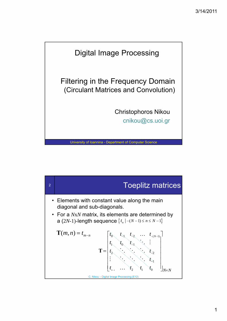
• Elements with constant value along the main diagonal and sub-diagonals.

• For a NxN matrix, its elements are determined by a (2N-1)-length sequence { }( 1) 1|n N n Nt − − ≤ ≤ −

( 1)0 1 2

1 0 1

Nt t t tt t t

− −− −⎡ ⎤⎢ ⎥⎢ ⎥

…( , ) m nm n t −=T

C. Nikou – Digital Image Processing (E12)

1

1 0 1

2 2

1

2 1 0N N N

t tt

t t t t−

−

−

−

×

⎢ ⎥⎢ ⎥=⎢ ⎥⎢ ⎥⎢ ⎥⎣ ⎦

T

…

3/14/2011

2

3 Toeplitz matrices (cont.)

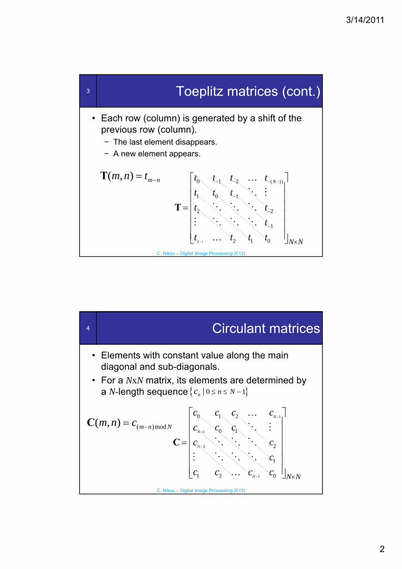
• Each row (column) is generated by a shift of the previous row (column).− The last element disappears.− A new element appears.

( 1)0 1 2

1 0 1

Nt t t tt t t

− −− −⎡ ⎤⎢ ⎥⎢ ⎥

…( , ) m nm n t −=T

C. Nikou – Digital Image Processing (E12)

1

1 0 1

2 2

1

2 1 0N N N

t tt

t t t t−

−

−

−

×

⎢ ⎥⎢ ⎥=⎢ ⎥⎢ ⎥⎢ ⎥⎣ ⎦

T

…

4 Circulant matrices

• Elements with constant value along the main diagonal and sub-diagonals.

• For a NxN matrix, its elements are determined by a N-length sequence { }0 1|n n Nc ≤ ≤ −

1

1

0 1 2

0 1

N

N

c c c cc c c

−

−

⎡ ⎤⎢ ⎥⎢ ⎥

…( )mod( , ) m n Nm n c −=C

C. Nikou – Digital Image Processing (E12)

2

1

2

1

1 2 0

N

N N N

c cc

c c c c

−

− ×

⎢ ⎥⎢ ⎥=⎢ ⎥⎢ ⎥⎢ ⎥⎣ ⎦

C

…

3/14/2011

3

5 Circulant matrices (cont.)

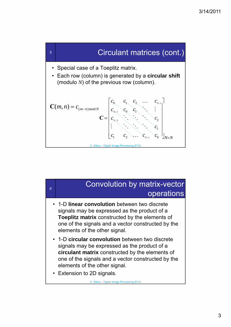
• Special case of a Toeplitz matrix.• Each row (column) is generated by a circular shift( ) g y

(modulo N) of the previous row (column).

1

1

0 1 2

0 1

N

N

c c c cc c c

−

−

⎡ ⎤⎢ ⎥⎢ ⎥

…( )mod( , ) m n Nm n c −=C

C. Nikou – Digital Image Processing (E12)

2

1

2

1

1 2 0

N

N N N

c cc

c c c c

−

− ×

⎢ ⎥⎢ ⎥=⎢ ⎥⎢ ⎥⎢ ⎥⎣ ⎦

C

…

6Convolution by matrix-vector

operations• 1-D linear convolution between two discrete

signals may be expressed as the product of a Toeplitz matrix constructed by the elements of one of the signals and a vector constructed by the elements of the other signal.

• 1-D circular convolution between two discrete signals may be expressed as the product of a

C. Nikou – Digital Image Processing (E12)

circulant matrix constructed by the elements of one of the signals and a vector constructed by the elements of the other signal.

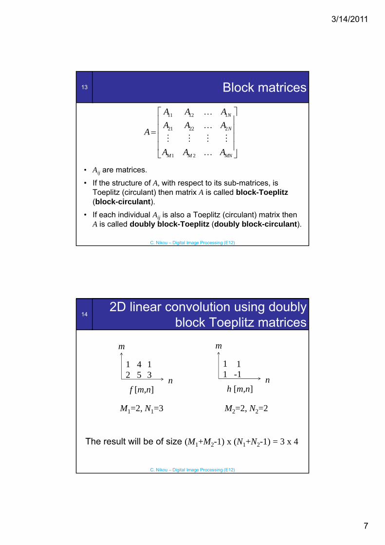
• Extension to 2D signals.

3/14/2011

4

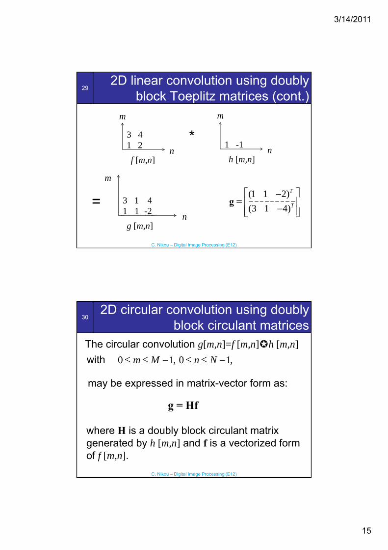
71D linear convolution using Toeplitz

matrices

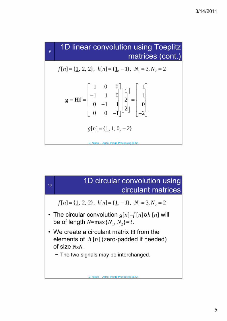
1 2[ ] {1, 2, 2}, [ ] {1, 1}, 3, 2f n h n N N= = − = =

• The linear convolution g[n]=f [n]*h [n] will be of length N=N1+N2-1=3+2-1=4.

• We create a Toeplitz matrix H from the elements of h [n] (zero-padded if needed) with

C. Nikou – Digital Image Processing (E12)

− N=4 lines (the length of the result).− N1=3 columns (the length of f [n]).− The two signals may be interchanged.

81D linear convolution using Toeplitz

matrices (cont.)

1 2[ ] {1, 2, 2}, [ ] {1, 1}, 3, 2f n h n N N= = − = =

1 0 01 1 00 1 10 0 1

⎡ ⎤⎢ ⎥−⎢ ⎥=⎢ ⎥−⎢ ⎥−⎣ ⎦

H Length of the result =4

Notice that H is not

C. Nikou – Digital Image Processing (E12)

4 30 0 1×⎣ ⎦

Length of f [n] = 3

Notice that H is not circulant (e.g. a -1 appears in the second line which is not present in the first line.

Zero-padded h[n] in the first column

3/14/2011

5

91D linear convolution using Toeplitz

matrices (cont.)

1 2[ ] {1, 2, 2}, [ ] {1, 1}, 3, 2f n h n N N= = − = =

1 0 0 11

1 1 0 12

0 1 1 02

⎡ ⎤ ⎡ ⎤⎡ ⎤⎢ ⎥ ⎢ ⎥− ⎢ ⎥⎢ ⎥ ⎢ ⎥= =⎢ ⎥⎢ ⎥ ⎢ ⎥−⎢ ⎥⎢ ⎥ ⎢ ⎥⎣ ⎦

g = Hf

C. Nikou – Digital Image Processing (E12)

0 0 1 2⎢ ⎥ ⎢ ⎥⎣ ⎦− −⎣ ⎦ ⎣ ⎦

[ ] {1, 1, 0, 2}g n = −

101D circular convolution using

circulant matrices

1 2[ ] {1, 2, 2}, [ ] {1, 1}, 3, 2f n h n N N= = − = =

• The circular convolution g[n]=f [n] h [n] will be of length N=max{N1, N2}=3.

• We create a circulant matrix H from the elements of h [n] (zero-padded if needed) f i

C. Nikou – Digital Image Processing (E12)

of size NxN.− The two signals may be interchanged.

3/14/2011

6

111D circular convolution using

circulant matrices (cont.)

1 2[ ] {1, 2, 2}, [ ] {1, 1}, 3, 2f n h n N N= = − = =

3 3

1 0 11 1 00 1 1

×

−⎡ ⎤⎢ ⎥= −⎢ ⎥⎢ ⎥−⎣ ⎦

H

C. Nikou – Digital Image Processing (E12)

Zero-padded h[n] in the first column

121D circular convolution using

circulant matrices (cont.)

1 2[ ] {1, 2, 2}, [ ] {1, 1}, 3, 2f n h n N N= = − = =

1 0 1 1 11 1 0 2 10 1 1 2 0

− −⎡ ⎤ ⎡ ⎤ ⎡ ⎤⎢ ⎥ ⎢ ⎥ ⎢ ⎥= − =⎢ ⎥ ⎢ ⎥ ⎢ ⎥⎢ ⎥ ⎢ ⎥ ⎢ ⎥−⎣ ⎦ ⎣ ⎦ ⎣ ⎦

g = Hf

C. Nikou – Digital Image Processing (E12)

[ ] { 1, 1, 0}g n == −

3/14/2011

7

13 Block matrices

11 12 1

21 22 2

N

N

A A AA A A

A

⎡ ⎤⎢ ⎥⎢ ⎥

……

• Aij are matrices.

• If the structure of A, with respect to its sub-matrices, is

21 22 2

1 2

N

M M MN

A

A A A

⎢ ⎥=⎢ ⎥⎢ ⎥⎣ ⎦…

C. Nikou – Digital Image Processing (E12)

Toeplitz (circulant) then matrix A is called block-Toeplitz(block-circulant).

• If each individual Aij is also a Toeplitz (circulant) matrix then A is called doubly block-Toeplitz (doubly block-circulant).

142D linear convolution using doubly

block Toeplitz matrices

m m

n

1 4 12 5 3f [m,n]

n

1 11 -1h [m,n]

M1=2, N1=3 M2=2, N2=2

C. Nikou – Digital Image Processing (E12)

The result will be of size (M1+M2-1) x (N1+N2-1) = 3 x 4

3/14/2011

8

152D linear convolution using doubly

block Toeplitz matrices (cont.) m

1 4 1

m

1 1

• At first, h[m,n] is zero-padded to 3 x 4 (the size of the m

0 0 0 0

n

1 4 12 5 3f [m,n]

n

1 11 -1h [m,n]

C. Nikou – Digital Image Processing (E12)

result).• Then, for each row of h[m,n],

a Toeplitz matrix with 3 columns (the number of columns of f [m,n]) is constructed.

n

1 1 01 -1 0

h[m,n]

00

0 0 0 0

162D linear convolution using doubly

block Toeplitz matrices (cont.) • For each row of h[m,n], a

Toeplitz matrix with 3 columns m

0 0 0 0(the number of columns of f [m,n]) is constructed.

n

1 1 01 -1 0

h[m,n]

00

1 0 0⎡ ⎤⎢ ⎥

1 0 0⎡ ⎤⎢ ⎥

0 0 0⎡ ⎤⎢ ⎥

C. Nikou – Digital Image Processing (E12)

1

1 1 00 1 10 0 1

⎢ ⎥−⎢ ⎥=⎢ ⎥−⎢ ⎥−⎣ ⎦

H 2

1 1 00 1 10 0 1

⎢ ⎥⎢ ⎥=⎢ ⎥⎢ ⎥⎣ ⎦

H 3

0 0 00 0 00 0 0

⎢ ⎥⎢ ⎥=⎢ ⎥⎢ ⎥⎣ ⎦

H

3/14/2011

9

172D linear convolution using doubly

block Toeplitz matrices (cont.) m

1 4 1

m

1 1

• Using matrices H1, H2and H3 as elements, a

n

1 4 12 5 3f [m,n]

n

1 11 -1h [m,n]

1 3⎡ ⎤⎢ ⎥H H

C. Nikou – Digital Image Processing (E12)

doubly block Toeplitzmatrix H is then constructed with 2 columns (the number of rows of f [m,n]).

2 1

3 2 12 6×

⎢ ⎥= ⎢ ⎥⎢ ⎥⎣ ⎦

H H HH H

182D linear convolution using doubly

block Toeplitz matrices (cont.) m

1 4 1

m

1 1

• We now construct

n

1 4 12 5 3f [m,n]

n

1 11 -1h [m,n]

25

(2 5 3)3 T

⎡ ⎤⎢ ⎥⎢ ⎥

⎡ ⎤⎢ ⎥

C. Nikou – Digital Image Processing (E12)

• We now construct a vector from the elements of f [m,n].

(2 5 3)3(1 4 1)1

41

T

T

⎡ ⎤⎢ ⎥= = ⎢ ⎥⎢ ⎥

⎢ ⎥⎢ ⎥ ⎣ ⎦⎢ ⎥⎢ ⎥⎣ ⎦

f

3/14/2011

10

192D linear convolution using doubly

block Toeplitz matrices (cont.) m

1 4 1

m

1 1

n

1 4 12 5 3f [m,n]

n

1 11 -1h [m,n]

1 3

25⎡ ⎤⎢ ⎥⎢ ⎥⎡ ⎤⎢ ⎥

H H

C. Nikou – Digital Image Processing (E12)

1 3

2 1

3 2

3141

⎡ ⎤⎢ ⎥⎢ ⎥= ⎢ ⎥⎢ ⎥⎢ ⎥⎢ ⎥⎣ ⎦ ⎢ ⎥⎢ ⎥⎣ ⎦

g = Hf H HH H

202D linear convolution using doubly

block Toeplitz matrices (cont.) 1 0 0 0 0 0 21 1 0 0 0 0 30 1 1 0 0 0 2

⎡ ⎤ ⎡ ⎤⎢ ⎥ ⎢ ⎥−⎢ ⎥ ⎢ ⎥⎢ ⎥ ⎢ ⎥0 1 1 0 0 0 2

0 0 1 0 0 0 2 31 0 0 1 0 0 5 3

(1 1 0 1 1 0 3 100 1 1 0 1 1 1 50 0 1 0 0 1 4 2

⎢ ⎥ ⎢ ⎥− −⎢ ⎥ ⎢ ⎥− ⎡ ⎤⎢ ⎥ ⎢ ⎥

⎢ ⎥⎢ ⎥ ⎢ ⎥⎢ ⎥⎢ ⎥ ⎢ ⎥⎢ ⎥−⎢ ⎥ ⎢ ⎥= = =⎢ ⎥⎢ ⎥ ⎢ ⎥− ⎢ ⎥⎢ ⎥ ⎢ ⎥⎢ ⎥−⎢ ⎥ ⎢ ⎥

g = Hf2 3 2 3)

(3 10 5 2)(1 5 5 1)

T

T

T

⎡ ⎤−⎢ ⎥⎢ ⎥⎢ ⎥⎣ ⎦

C. Nikou – Digital Image Processing (E12)

0 0 1 0 0 1 4 20 0 0 1 0 0 1 10 0 0 1 1 0 50 0 0 0 1 1 50 0 0 0 0 1 1

⎢ ⎥⎢ ⎥ ⎢ ⎥⎢ ⎥⎢ ⎥ ⎢ ⎥⎣ ⎦⎢ ⎥ ⎢ ⎥

⎢ ⎥ ⎢ ⎥⎢ ⎥ ⎢ ⎥⎢ ⎥ ⎢ ⎥⎢ ⎥ ⎢ ⎥⎣ ⎦ ⎣ ⎦

3/14/2011

11

212D linear convolution using doubly

block Toeplitz matrices (cont.)

*

m

1 4 1

m

1 1*n

1 4 12 5 3f [m,n]

n

1 11 -1h [m,n]

m1 5 5 1 (2 3 2 3)T⎡ ⎤

C. Nikou – Digital Image Processing (E12)

=32

n

3 10 52 3 -2g [m,n]

1 5 5 1 (2 3 2 3)(3 10 5 2)(1 5 5 1)

T

T

T

⎡ ⎤−⎢ ⎥⎢ ⎥⎢ ⎥⎣ ⎦

g =

222D linear convolution using doubly

block Toeplitz matrices (cont.)

m

Another example

m

n

3 41 2f [m,n]

m

n1 -1h [m,n]

C. Nikou – Digital Image Processing (E12)

M1=2, N1=2 M2=1, N2=2

The result will be of size (M1+M2-1) x (N1+N2-1) = 2 x 3

3/14/2011

12

232D linear convolution using doubly

block Toeplitz matrices (cont.) m m

• At first, h[m,n] is zero-padded to 2 x 3 (the size of the m

n

3 41 2f [m,n]

n1 -1h [m,n]

C. Nikou – Digital Image Processing (E12)

result).• Then, for each line of h[m,n],

a Toeplitz matrix with 2 columns (the number of columns of f [m,n]) is constructed.

n

0 0 01 -1 0

h[m,n]

242D linear convolution using doubly

block Toeplitz matrices (cont.) • For each row of h[m,n], a Toeplitz

matrix with 2 columns (the m

number of columns of f [m,n]) is constructed.

n

0 0 01 -1 0

h[m,n]

1 0⎡ ⎤ 0 0⎡ ⎤

C. Nikou – Digital Image Processing (E12)

1

1 01 10 1

⎡ ⎤⎢ ⎥= −⎢ ⎥⎢ ⎥−⎣ ⎦

H 2

0 00 00 0

⎡ ⎤⎢ ⎥= ⎢ ⎥⎢ ⎥⎣ ⎦

H

3/14/2011

13

252D linear convolution using doubly

block Toeplitz matrices (cont.) m m

• Using matrices H1 and H2 as elements, a

⎡ ⎤H H

n

3 41 2f [m,n]

n1 -1h [m,n]

C. Nikou – Digital Image Processing (E12)

doubly block Toeplitzmatrix H is then constructed with 2 columns (the number of rows of f [m,n]).

1 2

2 1 6 4×

⎡ ⎤= ⎢ ⎥⎣ ⎦

H HH

H H

262D linear convolution using doubly

block Toeplitz matrices (cont.) m m

1(1 2)2 T

⎡ ⎤⎢ ⎥ ⎡ ⎤

n

3 41 2f [m,n]

n1 -1h [m,n]

C. Nikou – Digital Image Processing (E12)

• We now construct a vector from the elements of f [m,n].

(1 2)2(3 4)3

4

T

T

⎢ ⎥ ⎡ ⎤⎢ ⎥= = ⎢ ⎥⎢ ⎥ ⎢ ⎥⎣ ⎦⎢ ⎥⎣ ⎦

f

3/14/2011

14

272D linear convolution using doubly

block Toeplitz matrices (cont.) m m

n

3 41 2f [m,n]

n1 -1h [m,n]

1⎡ ⎤⎢ ⎥

C. Nikou – Digital Image Processing (E12)

1 2

2 1

234

⎢ ⎥⎡ ⎤ ⎢ ⎥= ⎢ ⎥ ⎢ ⎥⎣ ⎦⎢ ⎥⎣ ⎦

H Hg = Hf

H H

282D linear convolution using doubly

block Toeplitz matrices (cont.)

1 0 0 0 1⎡ ⎤ ⎡ ⎤1 0 0 0 11 1 0 0 1 1

(1 1 2)0 1 0 0 2 2(3 1 4)0 0 1 0 3 3

0 0 1 1 4 1

T

T

⎡ ⎤ ⎡ ⎤⎢ ⎥ ⎢ ⎥− ⎡ ⎤⎢ ⎥ ⎢ ⎥⎢ ⎥ ⎡ ⎤−⎢ ⎥ ⎢ ⎥− −⎢ ⎥= = = ⎢ ⎥⎢ ⎥ ⎢ ⎥ −⎢ ⎥ ⎢ ⎥⎢ ⎥ ⎢ ⎥ ⎣ ⎦⎢ ⎥⎢ ⎥ ⎢ ⎥⎣ ⎦

g = Hf

C. Nikou – Digital Image Processing (E12)

0 0 1 1 4 10 0 0 1 4

⎢ ⎥ ⎢ ⎥− ⎣ ⎦⎢ ⎥ ⎢ ⎥− −⎣ ⎦ ⎣ ⎦

3/14/2011

15

292D linear convolution using doubly

block Toeplitz matrices (cont.)

*m m

*

m

n

3 41 2f [m,n]

n1 -1h [m,n]

T⎡ ⎤

C. Nikou – Digital Image Processing (E12)

=n

3 1 41 1 -2g [m,n]

(1 1 2)(3 1 4)

T

T

⎡ ⎤−⎢ ⎥−⎢ ⎥⎣ ⎦

g =

302D circular convolution using doubly

block circulant matrices

0 1 0 1m M n N≤ ≤ ≤ ≤The circular convolution g[m,n]=f [m,n] h [m,n]with 0 1, 0 1,m M n N≤ ≤ − ≤ ≤ −

may be expressed in matrix-vector form as:

g = Hf

with

C. Nikou – Digital Image Processing (E12)

where H is a doubly block circulant matrix generated by h [m,n] and f is a vectorized form of f [m,n].

3/14/2011

16

312D circular convolution using doubly

block circulant matrices (cont.)

0 1 2 1M M− −⎡ ⎤⎢ ⎥⎢ ⎥

H H H HH H H H

…

1 0 1 2

2 1 0 3

1 2 3 0

M

M M M

−

− − −

⎢ ⎥⎢ ⎥⎢ ⎥=⎢ ⎥⎢ ⎥⎢ ⎥⎣ ⎦

H H H HH H H H H

H H H H

…………

C. Nikou – Digital Image Processing (E12)

Each Hj, for j=1,..M, is a circulant matrix with N columns (the number of columns of f [m,n]) generated from the elements of the j-th row of h [m,n].

322D circular convolution using doubly

block circulant matrices (cont.)

[ 0] [ 1] [ 1]h j h j N h j⎡ ⎤[ ,0] [ , 1] [ ,1][ ,1] [ ,0] [ ,2]

[ , 1] [ , 2] [ ,0]

j

N N

h j h j N h jh j h j h j

h j N h j N h j ×

−⎡ ⎤⎢ ⎥⎢ ⎥=⎢ ⎥⎢ ⎥− −⎣ ⎦

H

……

…

C. Nikou – Digital Image Processing (E12)

Each Hj, for j=1,..M, is a NxN circulant matrix generated from the elements of the j-th row of h [m,n].

3/14/2011

17

332D circular convolution using doubly

block circulant matrices (cont.)

m m0 1 0 0 0 0

n

1 3 -11 2 1f [m,n]

n

1 01 -1h [m,n]

0 1 0

00

⎡ ⎤ ⎡ ⎤ 0 0 0⎡ ⎤

C. Nikou – Digital Image Processing (E12)

0

1 0 11 1 00 1 1

−⎡ ⎤⎢ ⎥= −⎢ ⎥⎢ ⎥−⎣ ⎦

H 1

1 0 00 1 00 0 1

⎡ ⎤⎢ ⎥= ⎢ ⎥⎢ ⎥⎣ ⎦

H 2

0 0 00 0 00 0 0

⎡ ⎤⎢ ⎥= ⎢ ⎥⎢ ⎥⎣ ⎦

H

342D circular convolution using doubly

block circulant matrices (cont.)

m m0 1 0 0 0 0

n

1 3 -11 2 1f [m,n]

n

1 01 -1h [m,n]

0 1 0

00

( )1 2 1 T⎡ ⎤⎡ ⎤ ⎢ ⎥H H H

C. Nikou – Digital Image Processing (E12)

( )( )( )

0 2 1

1 0 2

2 1 0

1 2 1

1 3 1

0 1 0

T

T

⎡ ⎤ ⎢ ⎥⎢ ⎥ ⎢ ⎥= −⎢ ⎥ ⎢ ⎥⎢ ⎥⎣ ⎦ ⎢ ⎥⎣ ⎦

H H Hg = Hf H H H

H H H

3/14/2011

18

352D circular convolution using doubly

block circulant matrices (cont.) 1 0 1 0 0 0 1 0 0 1 01 1 1 0 0 0 0 1 0 2 2

−⎡ ⎤ ⎡ ⎤ ⎡ ⎤⎢ ⎥ ⎢ ⎥ ⎢ ⎥1 1 1 0 0 0 0 1 0 2 2

0 1 0 0 0 0 0 0 1 1 11 0 0 1 0 1 0 0 0 1 30 1 0 1 1 1 0 0 0 3 40 0 1 0 1 0 0 0 0 1 30 0 0 0 0 0 1 0 1 0 1

⎢ ⎥ ⎢ ⎥ ⎢ ⎥−⎢ ⎥ ⎢ ⎥ ⎢ ⎥⎢ ⎥ ⎢ ⎥ ⎢ ⎥− −⎢ ⎥ ⎢ ⎥ ⎢ ⎥−⎢ ⎥ ⎢ ⎥ ⎢ ⎥⎢ ⎥ ⎢ ⎥ ⎢ ⎥= =−⎢ ⎥ ⎢ ⎥ ⎢ ⎥

− − −⎢ ⎥ ⎢ ⎥ ⎢ ⎥⎢ ⎥ ⎢ ⎥ ⎢ ⎥

g = Hf

C. Nikou – Digital Image Processing (E12)

0 0 0 0 0 0 1 0 1 0 10 0 0 0 0 0 1 1 1 1 40 0 0 0 0 0 0 1 0 0 2

⎢ ⎥ ⎢ ⎥ ⎢ ⎥−⎢ ⎥ ⎢ ⎥ ⎢ ⎥

−⎢ ⎥ ⎢ ⎥ ⎢⎢ ⎥ ⎢ ⎥ ⎢− −⎣ ⎦ ⎣ ⎦ ⎣ ⎦

⎥⎥

362D circular convolution using doubly

block circulant matrices (cont.) m

0 0 0m0 1 0

n

1 01 -1h [m,n]

m

00

n

1 3 -11 2 1f [m,n]

0 1 0

( )0 2 1 T⎡ ⎤

C. Nikou – Digital Image Processing (E12)

m

n

3 4 -30 2 -1g [m,n]

1 4 -2=( )( )( )

0 2 1

3 4 3

1 4 2

T

T

⎡ ⎤−⎢ ⎥⎢ ⎥−⎢ ⎥

−⎢ ⎥⎣ ⎦

g =

3/14/2011

19

37 Diagonalization of circulant matrices

Theorem: The columns of the inverse DFT matrix are eigenvectors of any circulant matrix. The corresponding eigenvalues are the DFT values of the signal generating the circulant matrix.Proof: Let

2 2 nj j knkw e w eπ π

− −Ν Ν= ⇔ =

C. Nikou – Digital Image Processing (E12)

N Nw e w eΝ Ν= ⇔ =

be the DFT basis elements of length N with:

0 1, 0 1,k N n N≤ ≤ − ≤ ≤ −

38Diagonalization of circulant matrices

(cont.)We know that the DFT F [k] of a 1D signal f [n]

may be expressed in matrix-vector form:may be expressed in matrix vector form:

whereF = Af

[ ] [ ][0], [1],..., [ 1] , [0], [1],..., [ 1]T Tf f f N F F F N− −f = F =

( ) ( ) ( ) ( )0 1 2 10 0 0 0 N

N N N Nw w w w−⎡ ⎤

⎢ ⎥…

C. Nikou – Digital Image Processing (E12)

( ) ( ) ( ) ( )( ) ( ) ( ) ( )

( ) ( ) ( ) ( )

0 1 2 11 1 1 1

0 1 2 11 1 1 1

N N N N

N

N N N N

NN N N NN N N N

w w w w

w w w w

−

−− − − −

⎢ ⎥⎢ ⎥⎢ ⎥=⎢ ⎥⎢ ⎥⎢ ⎥⎣ ⎦

A …

…

3/14/2011

20

39Diagonalization of circulant matrices

(cont.)The inverse DFT is then expressed by:

-1f = A F

where

f = A F

( )

( ) ( ) ( ) ( )( ) ( ) ( ) ( )

*0 1 2 10 0 0 0

0 1 2 11 1 1 11 *1 1

TN

N N N N

NT N N N N

w w w w

w w w wN N

−

−

−

⎛ ⎞⎡ ⎤⎜ ⎟⎢ ⎥⎜ ⎟⎢ ⎥⎜ ⎟⎢ ⎥= = ⎜ ⎟⎢ ⎥⎜ ⎟⎢ ⎥⎜ ⎟

A A

…

…

C. Nikou – Digital Image Processing (E12)

( ) ( ) ( ) ( )0 1 2 11 1 1 1 NN N N NN N N Nw w w w

−− − − −⎢ ⎥⎜ ⎟⎢ ⎥⎜ ⎟⎣ ⎦⎝ ⎠

…

The theorem implies that any circulant matrix has eigenvectors the columns of A-1.

40Diagonalization of circulant matrices

(cont.)Let H be a NxN circulant matrix generated by the 1D N-length signal h[n], that is:

[ ]mod( , ) ( ) [ ]N Nm n h m n h m n= − −H

Let also αk be the k-th column of the inverse DFT matrix A-1. We will prove that αk for any k is an eigenvector of H

C. Nikou – Digital Image Processing (E12)

We will prove that αk, for any k, is an eigenvector of H.The m-th element of the vector Hαk, denoted by is the result of the circular convolution of the signal h[n] with αk.

[ ]k mHα

3/14/2011

21

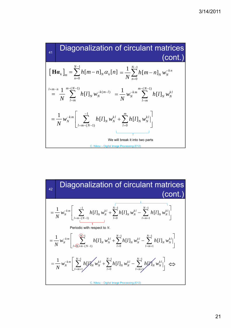
41Diagonalization of circulant matrices

(cont.)

[ ]1

0

[ ] [ ]N

k N kmn

h m n nα−

= −∑Hα1

0

1 [ ]N

k nN Nh m n w

N

−−= −∑

0n= 0nN =

( 1)( )1 [ ]

m Nl m nk m l

N Nl m

h l wN

− −= −− −

=

= ∑( 1)1 [ ]

m Nk m k l

N N Nl m

w h l wN

− −−

=

= ∑

11 ⎡ ⎤

C. Nikou – Digital Image Processing (E12)

1

( 1) 0

1 [ ] [ ]m

k m k l k lN N N N N

l m N l

w h l w h l wN

−−

= − − =

⎡ ⎤= +⎢ ⎥

⎣ ⎦∑ ∑

We will break it into two parts

42Diagonalization of circulant matrices

(cont.)1 1 11 [ ] [ ] [ ]

N Nk m k l k l k l

N N N N N N Nw h l w h l w h l w− − −

− ⎡ ⎤= + −⎢ ⎥∑ ∑ ∑

( 1) 0 1

[ ] [ ] [ ]N N N N N N Nl m N l l mN = − − = = +⎢ ⎥⎣ ⎦∑ ∑ ∑

Periodic with respect to N.

1 1 1

( 1) 0 1

1 [ ] [ ] [ ]N N N

k m k l k l k lN N N N N N N

l N m N l l m

w h l w h l w h l wN

− − −−

= + − − = = +

⎡ ⎤= + −⎢ ⎥

⎣ ⎦∑ ∑ ∑

C. Nikou – Digital Image Processing (E12)

1 1 1

1 0 1

1 [ ] [ ] [ ]N N N

k m k l k l k lN N N N N N N

l m l l mw h l w h l w h l w

N

− − −−

= + = = +

⎡ ⎤= + −⎢ ⎥⎣ ⎦∑ ∑ ∑ ⇔

3/14/2011

22

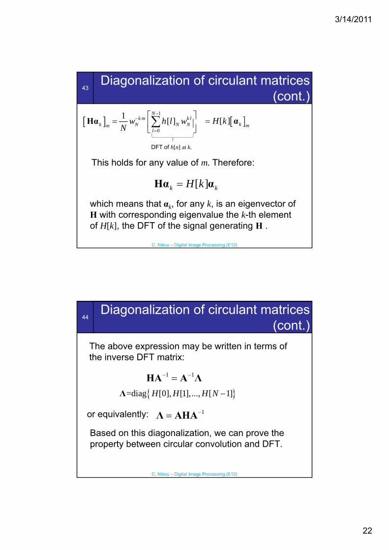
43Diagonalization of circulant matrices

(cont.)

[ ]1

0

1 [ ]N

k m k lk N N Nm

lw h l w

N

−−

=

⎡ ⎤= ⎢ ⎥⎣ ⎦∑Hα [ ][ ] k m

H k= α0lN =⎣ ⎦

DFT of h[n] at k.

This holds for any value of m. Therefore:

[ ]k kH k=Hα α

C. Nikou – Digital Image Processing (E12)

k k

which means that αk, for any k, is an eigenvector of H with corresponding eigenvalue the k-th element of H[k], the DFT of the signal generating H .

44Diagonalization of circulant matrices

(cont.)The above expression may be written in terms of the inverse DFT matrix:the inverse DFT matrix:

1 1− −=HA A Λ{ }=diag [0], [1],..., [ 1]H H H N −Λ

or equivalently: 1−=Λ ΑHA

C. Nikou – Digital Image Processing (E12)

Based on this diagonalization, we can prove the property between circular convolution and DFT.

q y

3/14/2011

23

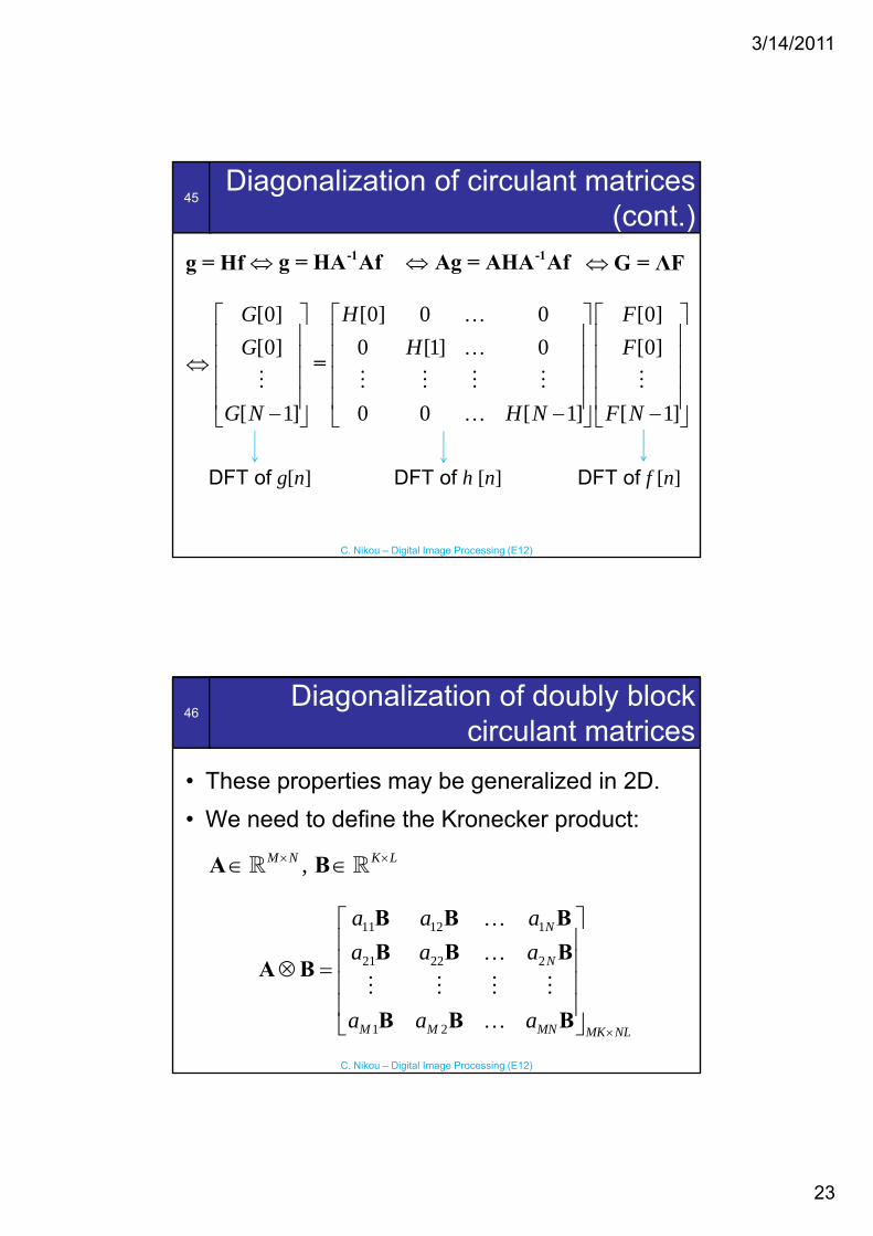
45Diagonalization of circulant matrices

(cont.)g = Hf ⇔ -1g = HA Af ⇔ -1Ag = AHA Af ⇔ G = ΛF

[0] [0] 0 0 [0][0] 0 [1] 0 [0]

[ 1] 0 0 [ 1] [ 1]

G H FG H F

G N H N F N

⎡ ⎤ ⎡ ⎤ ⎡ ⎤⎢ ⎥ ⎢ ⎥ ⎢ ⎥⎢ ⎥ ⎢ ⎥ ⎢ ⎥⇔⎢ ⎥ ⎢ ⎥ ⎢ ⎥⎢ ⎥ ⎢ ⎥ ⎢ ⎥− − −⎣ ⎦ ⎣ ⎦ ⎣ ⎦

=

……

…

C. Nikou – Digital Image Processing (E12)

DFT of g[n] DFT of f [n]DFT of h [n]

⎣ ⎦ ⎣ ⎦ ⎣ ⎦

46Diagonalization of doubly block

circulant matrices • These properties may be generalized in 2D.• We need to define the Kronecker product:

11 12 1Na a a⎡ ⎤⎢ ⎥

B B B…

,M N K L× ×∈ ∈A B

C. Nikou – Digital Image Processing (E12)

21 22 2

1 2

N

M M MN MK NL

a a a

a a a×

⎢ ⎥⎢ ⎥⊗ =⎢ ⎥⎢ ⎥⎣ ⎦

B B BA B

B B B

…

…

3/14/2011

24

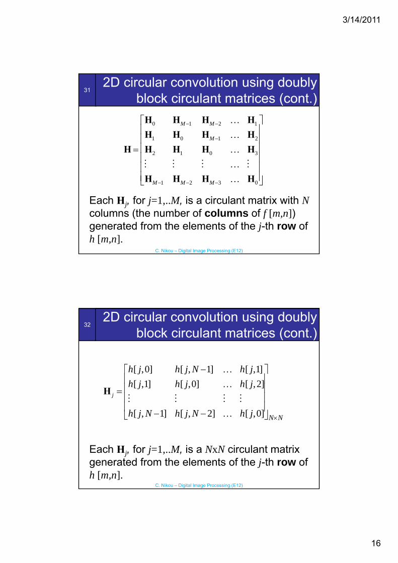
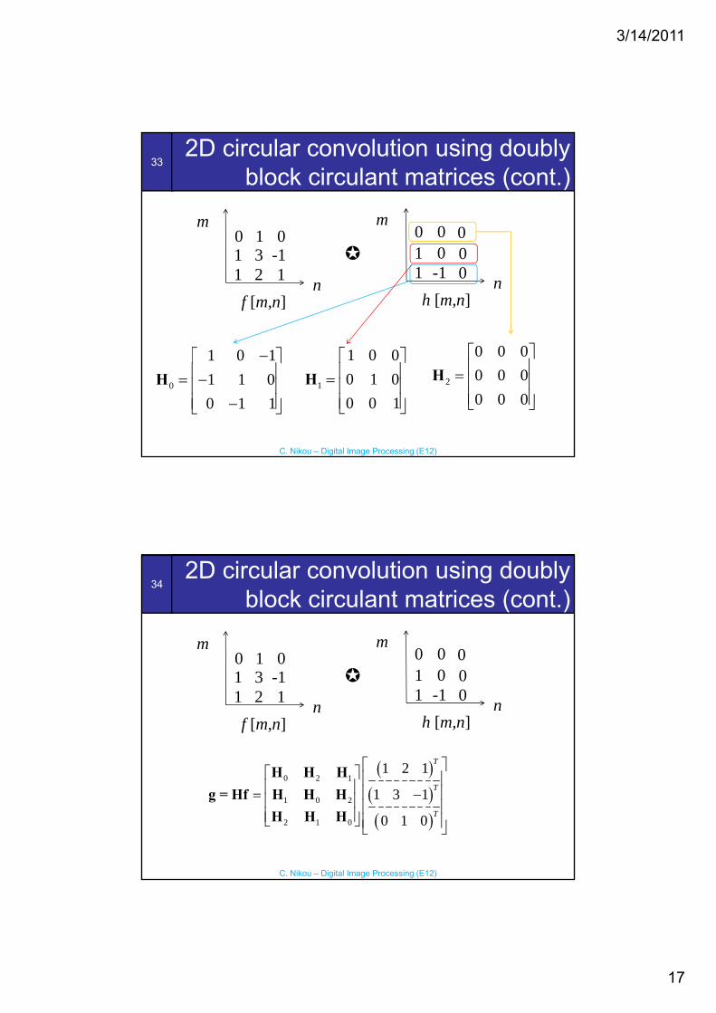
47Diagonalization of doubly block

circulant matrices (cont.) • The 2D signal f [m,n], 0 1, 0 1,m M n N≤ ≤ − ≤ ≤ −

may be vectorized in lexicographic ordering (stacking one column after the other) to a vector:

1MN×∈f

• The DFT of f [m n] may be obtained in

C. Nikou – Digital Image Processing (E12)

The DFT of f [m,n], may be obtained in matrix-vector form:

( )F = ⊗A A f

48Diagonalization of doubly block

circulant matrices (cont.) Theorem: The columns of the inverse 2D DFT matrix

( ) 1

are eigenvectors of any doubly block circulantmatrix. The corresponding eigenvalues are the 2D DFT values of the 2D signal generating the doubly block circulant matrix:

( ) 1−⊗A A

C. Nikou – Digital Image Processing (E12)

( ) ( ) 1−= ⊗ ⊗Λ A A H A A

block circulant matrix:

Doubly block circulantDiagonal, containing the 2D DFT of h[m,n] generating H