63
Chapter 21 Chapter 21 The Theory of The Theory of Consumer Consumer Choice Choice 002 by Nelson, a division of Thomson Canada Limited 002 by Nelson, a division of Thomson Canada Limited
| Date post: | 29-Dec-2015 |
| Category: |
Documents |
| Upload: | chad-gibson |
| View: | 216 times |
| Download: | 2 times |

Chapter 21Chapter 21Chapter 21Chapter 21
The Theory of The Theory of Consumer ChoiceConsumer Choice
The Theory of The Theory of Consumer ChoiceConsumer Choice
©© 2002 by Nelson, a division of Thomson Canada Limited 2002 by Nelson, a division of Thomson Canada Limited©© 2002 by Nelson, a division of Thomson Canada Limited 2002 by Nelson, a division of Thomson Canada Limited
Mankiw et al. Principles of Microeconomics, 2nd Canadian Edition Chapter 21: Page 2
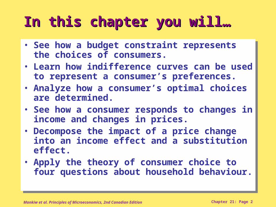
• See how a budget constraint represents the choices of consumers.
• Learn how indifference curves can be used to represent a consumer’s preferences.
• Analyze how a consumer’s optimal choices are determined.
• See how a consumer responds to changes in income and changes in prices.
• Decompose the impact of a price change into an income effect and a substitution effect.
• Apply the theory of consumer choice to four questions about household behaviour.
In this chapter you will…In this chapter you will…
Mankiw et al. Principles of Microeconomics, 2nd Canadian Edition Chapter 21: Page 3
The Theory of Consumer ChoiceThe Theory of Consumer Choice
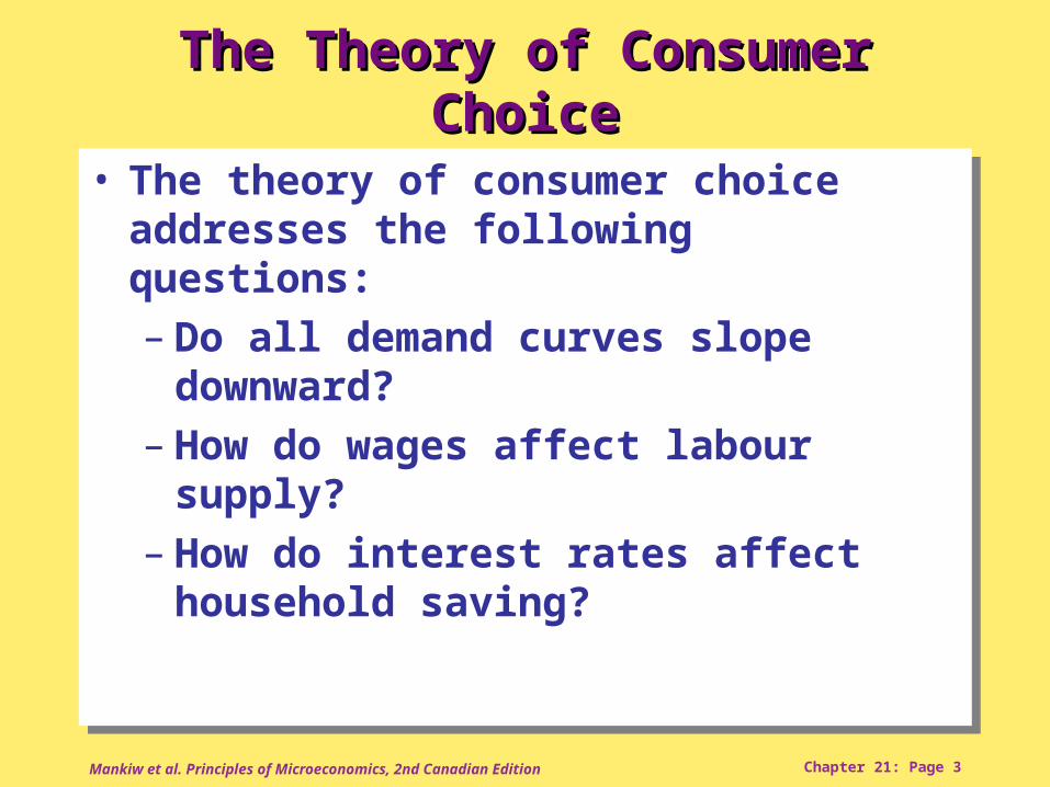
• The theory of consumer choice addresses the following questions:– Do all demand curves slope downward?– How do wages affect labour supply?– How do interest rates affect household
saving?
• The theory of consumer choice addresses the following questions:– Do all demand curves slope downward?– How do wages affect labour supply?– How do interest rates affect household
saving?
Mankiw et al. Principles of Microeconomics, 2nd Canadian Edition Chapter 21: Page 4
THE BUDGET CONSTRAINT: WHAT THE BUDGET CONSTRAINT: WHAT THE CONSUMER CAN AFFORDTHE CONSUMER CAN AFFORD
• The budget constraint depicts the limit on the consumption “bundles” that a consumer can afford.– People consume less than they desire
because their spending is constrained, or limited, by their income.
• The budget constraint depicts the limit on the consumption “bundles” that a consumer can afford.– People consume less than they desire
because their spending is constrained, or limited, by their income.

Mankiw et al. Principles of Microeconomics, 2nd Canadian Edition Chapter 21: Page 5
THE BUDGET CONSTRAINT: WHAT THE BUDGET CONSTRAINT: WHAT THE CONSUMER CAN AFFORDTHE CONSUMER CAN AFFORD
• The budget constraint shows the various combinations of goods the consumer can afford given his or her income and the prices of the two goods.
• The budget constraint shows the various combinations of goods the consumer can afford given his or her income and the prices of the two goods.
Mankiw et al. Principles of Microeconomics, 2nd Canadian Edition Chapter 21: Page 6
The Consumer’s Budget The Consumer’s Budget ConstraintConstraint
Mankiw et al. Principles of Microeconomics, 2nd Canadian Edition Chapter 21: Page 7
THE BUDGET CONSTRAINT: WHAT THE BUDGET CONSTRAINT: WHAT THE CONSUMER CAN AFFORD THE CONSUMER CAN AFFORD
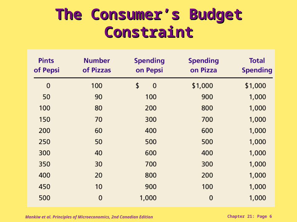
• The Consumer’s Budget Constraint– Any point on the budget constraint line
indicates the consumer’s combination or tradeoff between two goods.
– For example, if the consumer buys no pizzas, he can afford 500 pints of Pepsi (point B). If he buys no Pepsi, he can afford 100 pizzas (point A).
• The Consumer’s Budget Constraint– Any point on the budget constraint line
indicates the consumer’s combination or tradeoff between two goods.
– For example, if the consumer buys no pizzas, he can afford 500 pints of Pepsi (point B). If he buys no Pepsi, he can afford 100 pizzas (point A).
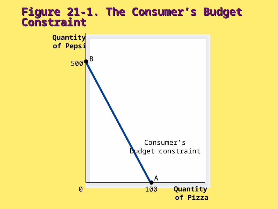
Figure 21-1. The Consumer’s Budget Figure 21-1. The Consumer’s Budget ConstraintConstraint
Quantityof Pizza
Quantityof Pepsi
0
Consumer’sbudget constraint
500B
100
A
Mankiw et al. Principles of Microeconomics, 2nd Canadian Edition Chapter 21: Page 9
THE BUDGET CONSTRAINT: WHAT THE BUDGET CONSTRAINT: WHAT THE CONSUMER CAN AFFORD THE CONSUMER CAN AFFORD
• The Consumer’s Budget Constraint– Alternately, the consumer can buy 50
pizzas and 250 pints of Pepsi.
• The Consumer’s Budget Constraint– Alternately, the consumer can buy 50
pizzas and 250 pints of Pepsi.

Quantityof Pizza
Quantityof Pepsi
0
Consumer’sbudget constraint
500B
250
50
C
100
A
Figure 21-1. The Consumer’s Budget Figure 21-1. The Consumer’s Budget ConstraintConstraint

Mankiw et al. Principles of Microeconomics, 2nd Canadian Edition Chapter 21: Page 11
THE BUDGET CONSTRAINT: WHAT THE BUDGET CONSTRAINT: WHAT THE CONSUMER CAN AFFORDTHE CONSUMER CAN AFFORD
• The slope of the budget constraint line equals the relative price of the two goods, that is, the price of one good compared to the price of the other.
• It measures the rate at which the consumer can trade one good for the other.
• The slope of the budget constraint line equals the relative price of the two goods, that is, the price of one good compared to the price of the other.
• It measures the rate at which the consumer can trade one good for the other.
Mankiw et al. Principles of Microeconomics, 2nd Canadian Edition Chapter 21: Page 12
PREFERENCES: WHAT THE PREFERENCES: WHAT THE CONSUMER WANTSCONSUMER WANTS
• A consumer’s preference among consumption bundles may be illustrated with indifference curves.
• A consumer’s preference among consumption bundles may be illustrated with indifference curves.
Mankiw et al. Principles of Microeconomics, 2nd Canadian Edition Chapter 21: Page 13
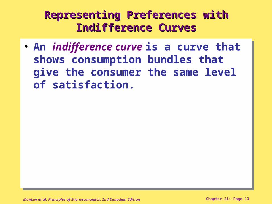
Representing Preferences with Indifference Representing Preferences with Indifference CurvesCurves
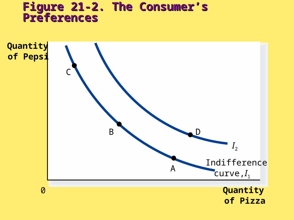
• An indifference curve is a curve that shows consumption bundles that give the consumer the same level of satisfaction.
• An indifference curve is a curve that shows consumption bundles that give the consumer the same level of satisfaction.

Figure 21-2. The Consumer’s PreferencesFigure 21-2. The Consumer’s Preferences
Quantityof Pizza
Quantityof Pepsi
0
Indifferencecurve, I1
I2
C
B
A
D
Mankiw et al. Principles of Microeconomics, 2nd Canadian Edition Chapter 21: Page 15
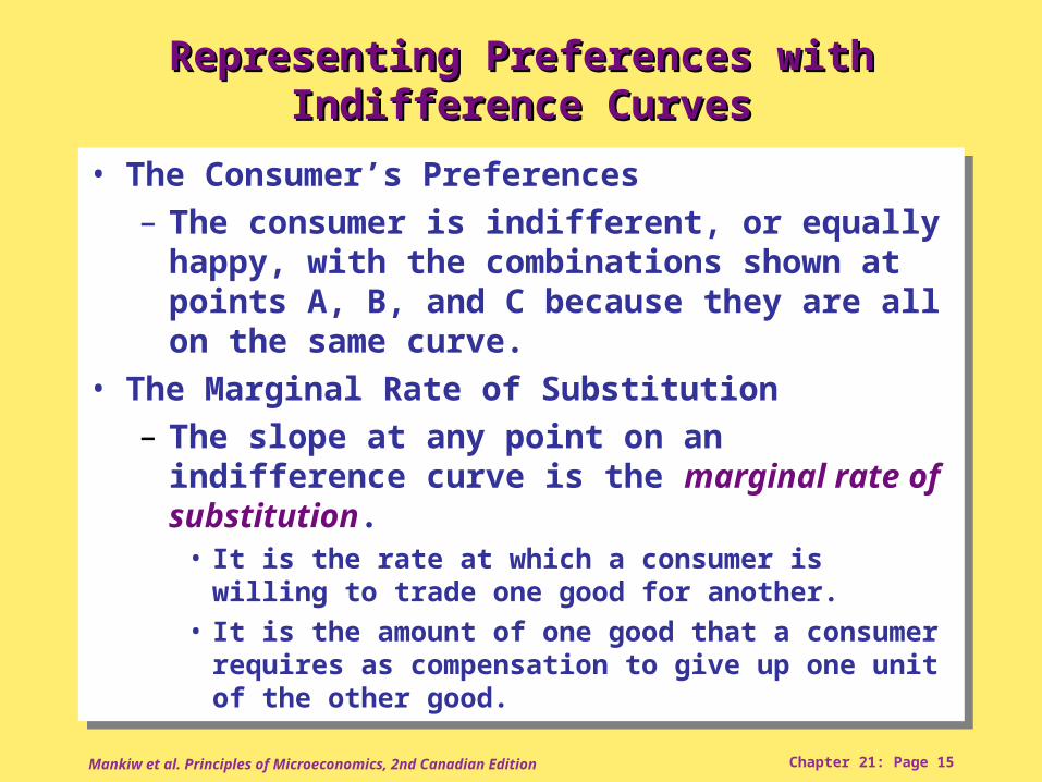
Representing Preferences with Indifference Representing Preferences with Indifference CurvesCurves
• The Consumer’s Preferences– The consumer is indifferent, or equally happy,
with the combinations shown at points A, B, and C because they are all on the same curve.
• The Marginal Rate of Substitution– The slope at any point on an indifference curve
is the marginal rate of substitution.• It is the rate at which a consumer is willing to trade
one good for another.• It is the amount of one good that a consumer
requires as compensation to give up one unit of the other good.

Quantityof Pizza
Quantityof Pepsi
0
Indifferencecurve, I1
I21
MRS
C
B
A
D
Figure 21-2. The Consumer’s PreferencesFigure 21-2. The Consumer’s Preferences
Mankiw et al. Principles of Microeconomics, 2nd Canadian Edition Chapter 21: Page 17
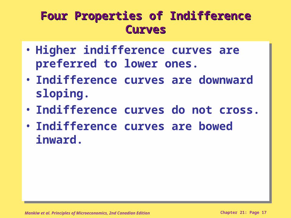
Four Properties of Indifference CurvesFour Properties of Indifference Curves
• Higher indifference curves are preferred to lower ones.
• Indifference curves are downward sloping.• Indifference curves do not cross.• Indifference curves are bowed inward.
• Higher indifference curves are preferred to lower ones.
• Indifference curves are downward sloping.• Indifference curves do not cross.• Indifference curves are bowed inward.
Mankiw et al. Principles of Microeconomics, 2nd Canadian Edition Chapter 21: Page 18
Four Properties of Indifference Curves Four Properties of Indifference Curves
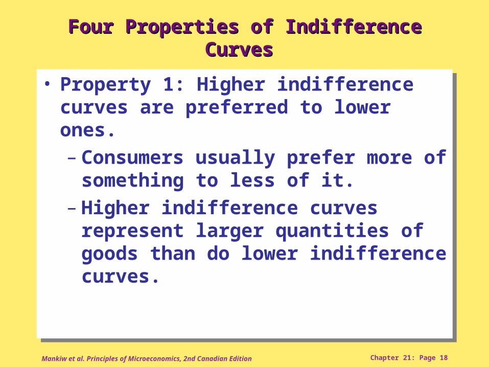
• Property 1: Higher indifference curves are preferred to lower ones.– Consumers usually prefer more of
something to less of it. – Higher indifference curves represent
larger quantities of goods than do lower indifference curves.
• Property 1: Higher indifference curves are preferred to lower ones.– Consumers usually prefer more of
something to less of it. – Higher indifference curves represent
larger quantities of goods than do lower indifference curves.
Quantityof Pizza
Quantityof Pepsi
0
Indifferencecurve, I1
I2
C
B
A
D
Figure 21-2. The Consumer’s PreferencesFigure 21-2. The Consumer’s Preferences

Mankiw et al. Principles of Microeconomics, 2nd Canadian Edition Chapter 21: Page 20
Four Properties of Indifference Curves Four Properties of Indifference Curves
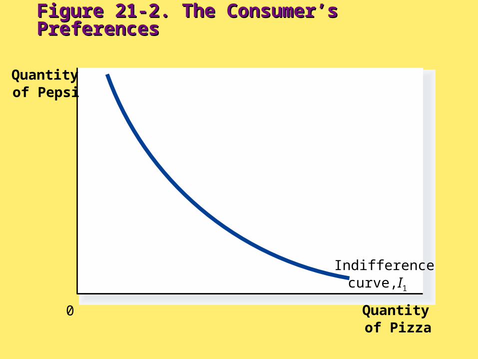
• Property 2: Indifference curves are downward sloping.– A consumer is willing to give up one
good only if he or she gets more of the other good in order to remain equally happy.
– If the quantity of one good is reduced, the quantity of the other good must increase.
– For this reason, most indifference curves slope downward.
Quantityof Pizza
Quantityof Pepsi
0
Indifferencecurve, I1
Figure 21-2. The Consumer’s PreferencesFigure 21-2. The Consumer’s Preferences
Mankiw et al. Principles of Microeconomics, 2nd Canadian Edition Chapter 21: Page 22
Four Properties of Indifference Curves Four Properties of Indifference Curves
• Property 3: Indifference curves do not cross.– Points A and B should make the
consumer equally happy.– Points B and C should make the
consumer equally happy.– This implies that A and C would make
the consumer equally happy.– But C has more of both goods
compared to A.
• Property 3: Indifference curves do not cross.– Points A and B should make the
consumer equally happy.– Points B and C should make the
consumer equally happy.– This implies that A and C would make
the consumer equally happy.– But C has more of both goods
compared to A.
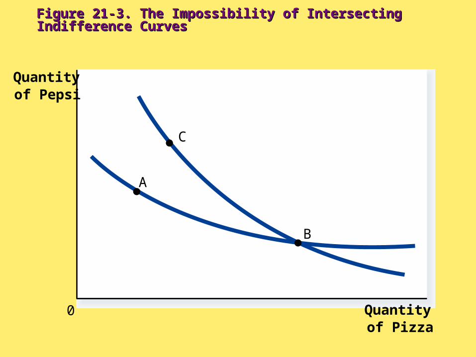
Figure 21-3. The Impossibility of Intersecting Indifference CurvesFigure 21-3. The Impossibility of Intersecting Indifference Curves
Quantityof Pizza
Quantityof Pepsi
0
C
A
B

Mankiw et al. Principles of Microeconomics, 2nd Canadian Edition Chapter 21: Page 24
Four Properties of Indifference Curves Four Properties of Indifference Curves
• Property 4: Indifference curves are bowed inward.– People are more willing to trade away
goods that they have in abundance and less willing to trade away goods of which they have little.
– These differences in a consumer’s marginal substitution rates cause his or her indifference curve to bow inward.
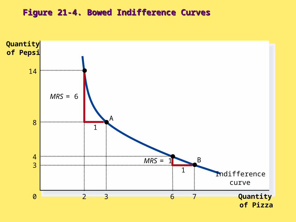
Figure 21-4. Bowed Indifference CurvesFigure 21-4. Bowed Indifference Curves
Quantityof Pizza
Quantityof Pepsi
0
Indifferencecurve
8
3
A
3
7
B
1
MRS = 6
1MRS = 14
6
14
2

Mankiw et al. Principles of Microeconomics, 2nd Canadian Edition Chapter 21: Page 26
Two Extreme Examples of Indifference Two Extreme Examples of Indifference CurvesCurves
• Perfect substitutes• Perfect complements
• Perfect substitutes• Perfect complements
Mankiw et al. Principles of Microeconomics, 2nd Canadian Edition Chapter 21: Page 27
Two Extreme Examples of Indifference Two Extreme Examples of Indifference Curves Curves
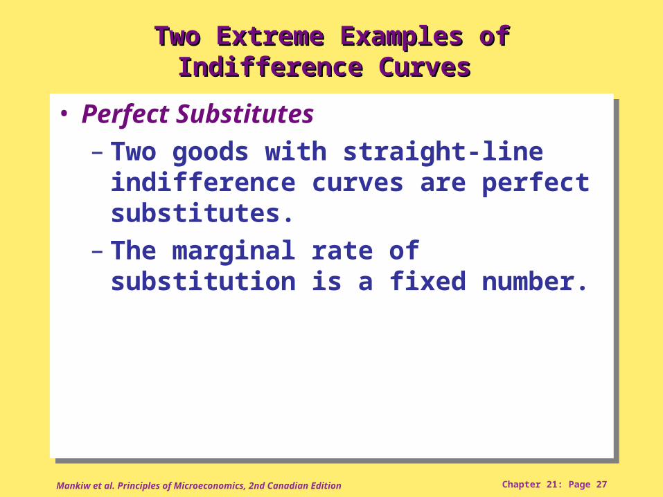
• Perfect Substitutes– Two goods with straight-line
indifference curves are perfect substitutes.
– The marginal rate of substitution is a fixed number.
• Perfect Substitutes– Two goods with straight-line
indifference curves are perfect substitutes.
– The marginal rate of substitution is a fixed number.
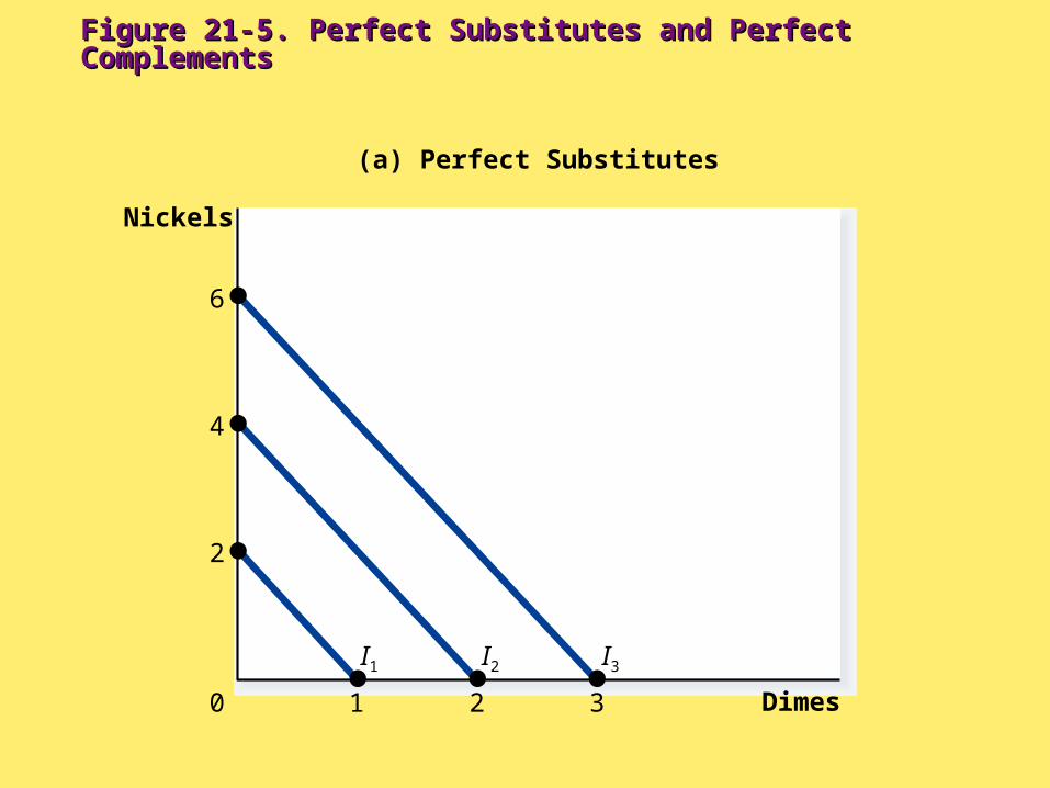
Figure 21-5. Perfect Substitutes and Perfect ComplementsFigure 21-5. Perfect Substitutes and Perfect Complements
Dimes0
Nickels
(a) Perfect Substitutes
I1 I2 I3
3
6
2
4
1
2

Mankiw et al. Principles of Microeconomics, 2nd Canadian Edition Chapter 21: Page 29
Two Extreme Examples of Indifference Two Extreme Examples of Indifference Curves Curves
• Perfect Complements– Two goods with right-angle indifference
curves are perfect complements.
• Perfect Complements– Two goods with right-angle indifference
curves are perfect complements.
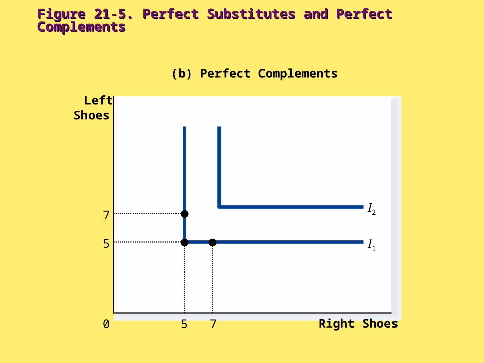
Figure 21-5. Perfect Substitutes and Perfect ComplementsFigure 21-5. Perfect Substitutes and Perfect Complements
Right Shoes0
LeftShoes
(b) Perfect Complements
I1
I2
7
7
5
5

Mankiw et al. Principles of Microeconomics, 2nd Canadian Edition Chapter 21: Page 31
OPTIMIZATION: WHAT THE OPTIMIZATION: WHAT THE CONSUMER CHOOSESCONSUMER CHOOSES
• Consumers want to get the combination of goods on the highest possible indifference curve.
• However, the consumer must also end up on or below his budget constraint.
• Consumers want to get the combination of goods on the highest possible indifference curve.
• However, the consumer must also end up on or below his budget constraint.

Mankiw et al. Principles of Microeconomics, 2nd Canadian Edition Chapter 21: Page 32
The Consumer’s Optimal ChoicesThe Consumer’s Optimal Choices
• Combining the indifference curve and the budget constraint determines the consumer’s optimal choice.
• Consumer optimum occurs at the point where the highest indifference curve and the budget constraint are tangent.
• Combining the indifference curve and the budget constraint determines the consumer’s optimal choice.
• Consumer optimum occurs at the point where the highest indifference curve and the budget constraint are tangent.
Mankiw et al. Principles of Microeconomics, 2nd Canadian Edition Chapter 21: Page 33
The Consumer’s Optimal ChoiceThe Consumer’s Optimal Choice
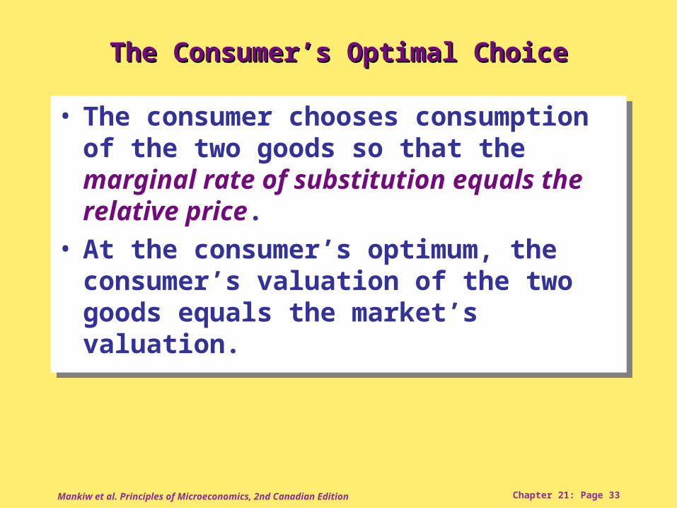
• The consumer chooses consumption of the two goods so that the marginal rate of substitution equals the relative price.
• At the consumer’s optimum, the consumer’s valuation of the two goods equals the market’s valuation.
• The consumer chooses consumption of the two goods so that the marginal rate of substitution equals the relative price.
• At the consumer’s optimum, the consumer’s valuation of the two goods equals the market’s valuation.
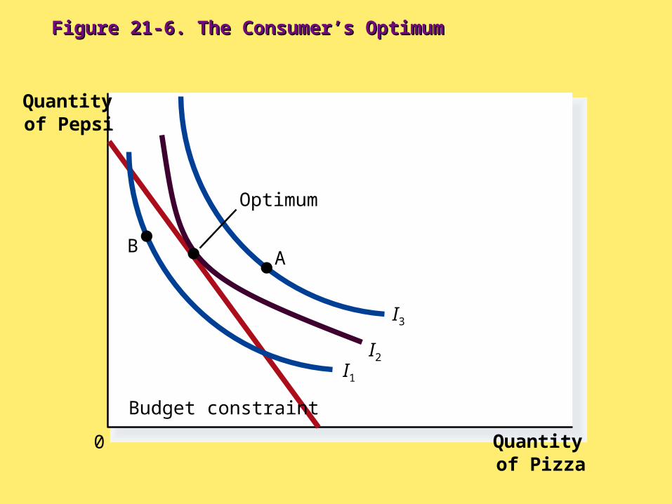
Figure 21-6. The Consumer’s OptimumFigure 21-6. The Consumer’s Optimum
Quantityof Pizza
Quantityof Pepsi
0
Budget constraint
I1I2
I3
Optimum
AB
Mankiw et al. Principles of Microeconomics, 2nd Canadian Edition Chapter 21: Page 35
How Changes in Income Affect the How Changes in Income Affect the Consumer’s ChoicesConsumer’s Choices
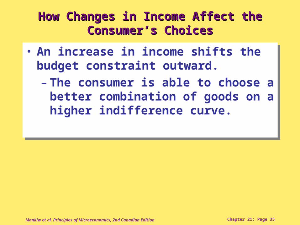
• An increase in income shifts the budget constraint outward.– The consumer is able to choose a better
combination of goods on a higher indifference curve.
• An increase in income shifts the budget constraint outward.– The consumer is able to choose a better
combination of goods on a higher indifference curve.
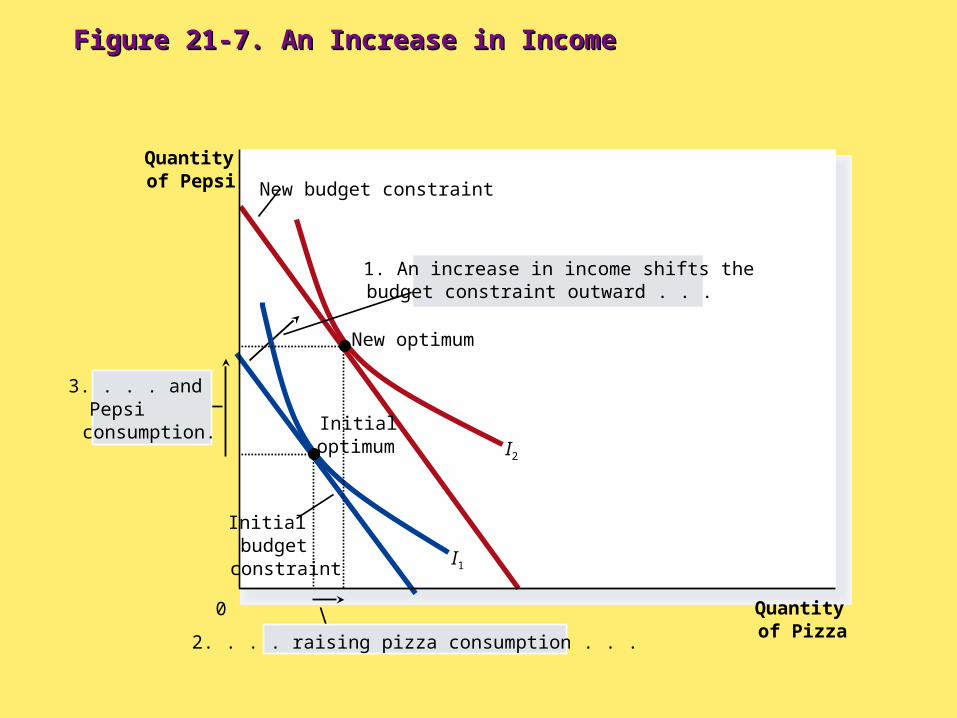
Figure 21-7. An Increase in IncomeFigure 21-7. An Increase in Income
Quantityof Pizza
Quantityof Pepsi
0
New budget constraint
I1
I2
2. . . . raising pizza consumption . . .
3. . . . andPepsiconsumption.
Initialbudgetconstraint
1. An increase in income shifts thebudget constraint outward . . .
Initialoptimum
New optimum
Mankiw et al. Principles of Microeconomics, 2nd Canadian Edition Chapter 21: Page 37
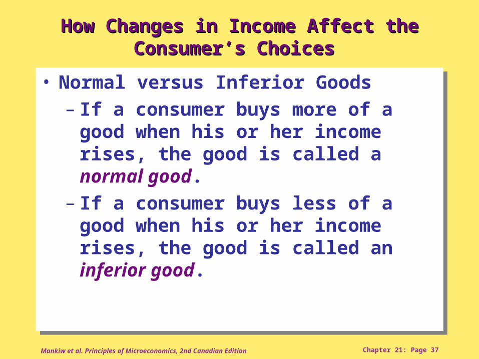
How Changes in Income Affect the How Changes in Income Affect the Consumer’s Choices Consumer’s Choices
• Normal versus Inferior Goods– If a consumer buys more of a good
when his or her income rises, the good is called a normal good.
– If a consumer buys less of a good when his or her income rises, the good is called an inferior good.
• Normal versus Inferior Goods– If a consumer buys more of a good
when his or her income rises, the good is called a normal good.
– If a consumer buys less of a good when his or her income rises, the good is called an inferior good.
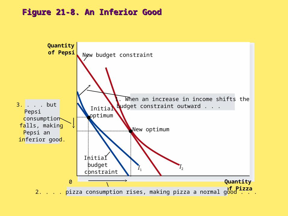
Figure 21-8. An Inferior GoodFigure 21-8. An Inferior Good
Quantityof Pizza
Quantityof Pepsi
0
Initialbudgetconstraint
New budget constraint
I1 I2
1. When an increase in income shifts thebudget constraint outward . . .3. . . . but
Pepsiconsumptionfalls, makingPepsi aninferior good.
2. . . . pizza consumption rises, making pizza a normal good . . .
Initialoptimum
New optimum

Mankiw et al. Principles of Microeconomics, 2nd Canadian Edition Chapter 21: Page 39
How Changes in Prices Affect Consumer’s How Changes in Prices Affect Consumer’s ChoicesChoices
• A fall in the price of any good rotates the budget constraint outward and changes the slope of the budget constraint.
• A fall in the price of any good rotates the budget constraint outward and changes the slope of the budget constraint.
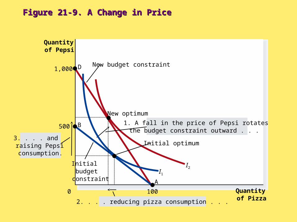
Figure 21-9. A Change in PriceFigure 21-9. A Change in Price
Quantityof Pizza
Quantityof Pepsi
0
1,000 D
500 B
100
A
I1I2
Initial optimum
New budget constraint
Initialbudgetconstraint
1. A fall in the price of Pepsi rotates the budget constraint outward . . .
3. . . . andraising Pepsiconsumption.
2. . . . reducing pizza consumption . . .
New optimum
Mankiw et al. Principles of Microeconomics, 2nd Canadian Edition Chapter 21: Page 41
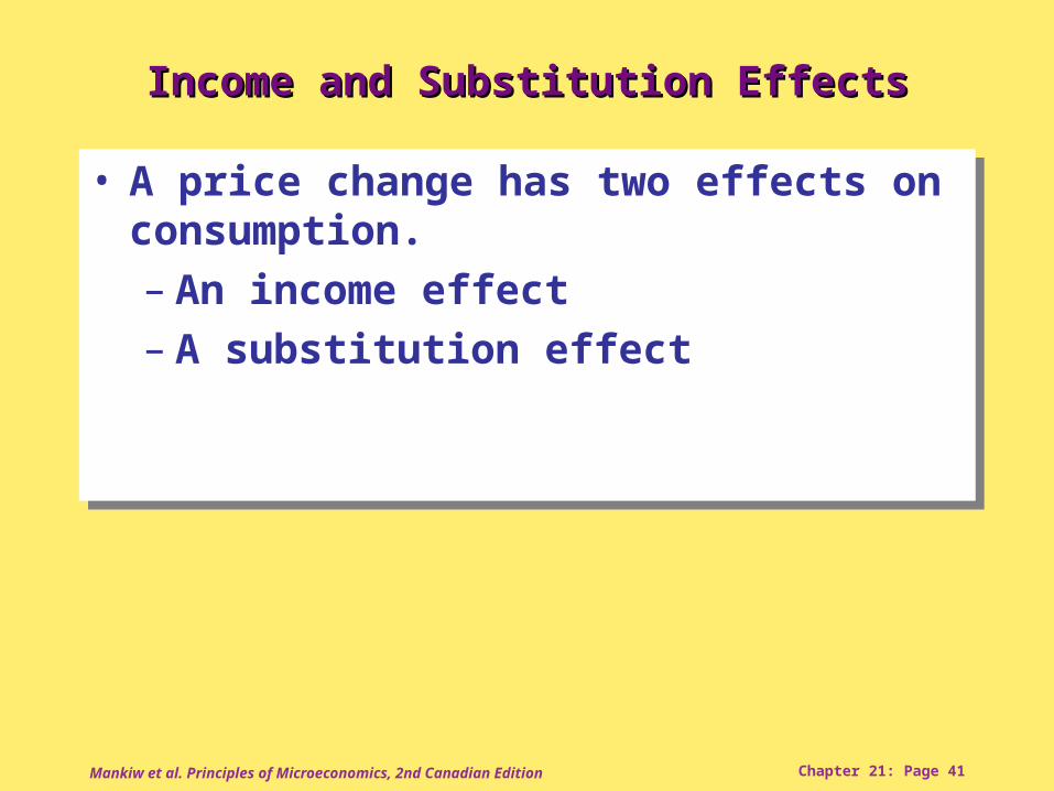
Income and Substitution EffectsIncome and Substitution Effects
• A price change has two effects on consumption.– An income effect– A substitution effect
• A price change has two effects on consumption.– An income effect– A substitution effect
Mankiw et al. Principles of Microeconomics, 2nd Canadian Edition Chapter 21: Page 42
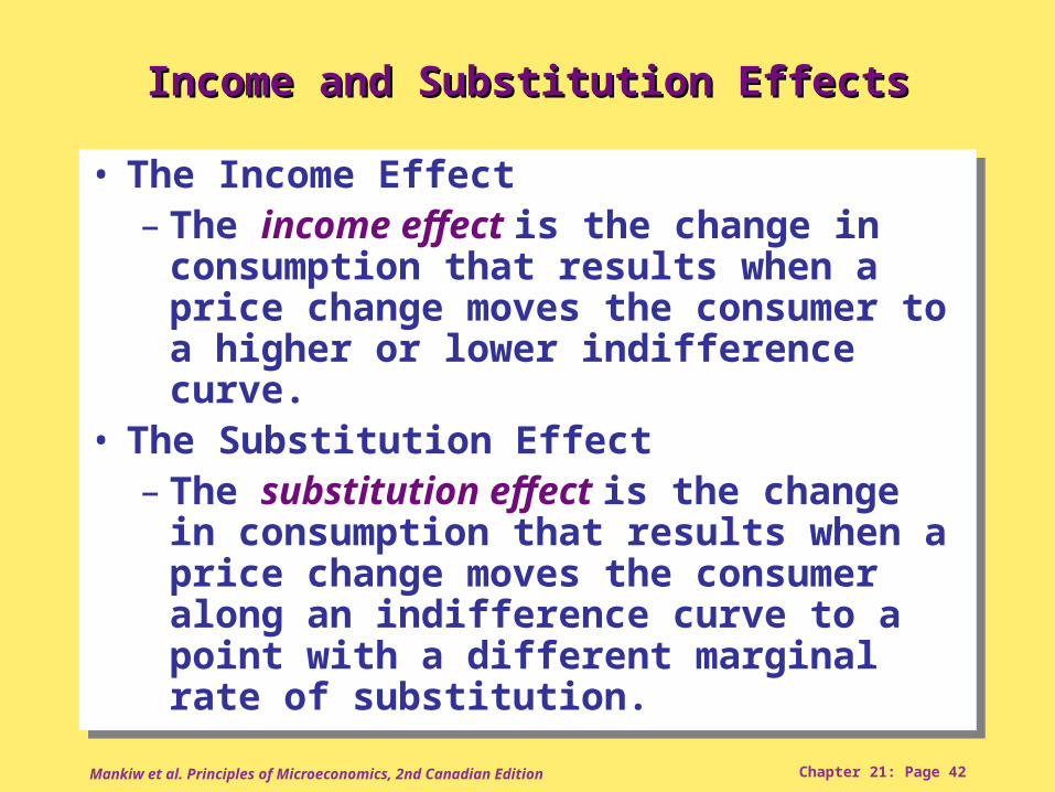
Income and Substitution EffectsIncome and Substitution Effects
• The Income Effect– The income effect is the change in
consumption that results when a price change moves the consumer to a higher or lower indifference curve.
• The Substitution Effect– The substitution effect is the change in
consumption that results when a price change moves the consumer along an indifference curve to a point with a different marginal rate of substitution.
Mankiw et al. Principles of Microeconomics, 2nd Canadian Edition Chapter 21: Page 43
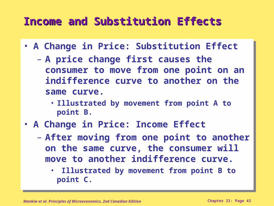
Income and Substitution EffectsIncome and Substitution Effects
• A Change in Price: Substitution Effect– A price change first causes the consumer to
move from one point on an indifference curve to another on the same curve.
• Illustrated by movement from point A to point B.
• A Change in Price: Income Effect – After moving from one point to another on the
same curve, the consumer will move to another indifference curve.
• Illustrated by movement from point B to point C.

Figure 21-10. Income and Substitution EffectsFigure 21-10. Income and Substitution Effects
Quantityof Pizza
Quantityof Pepsi
0
I1
I2A
Initial optimum
New budget constraint
Initialbudgetconstraint
Substitutioneffect
Substitution effect
Incomeeffect
Income effect
B
C New optimum
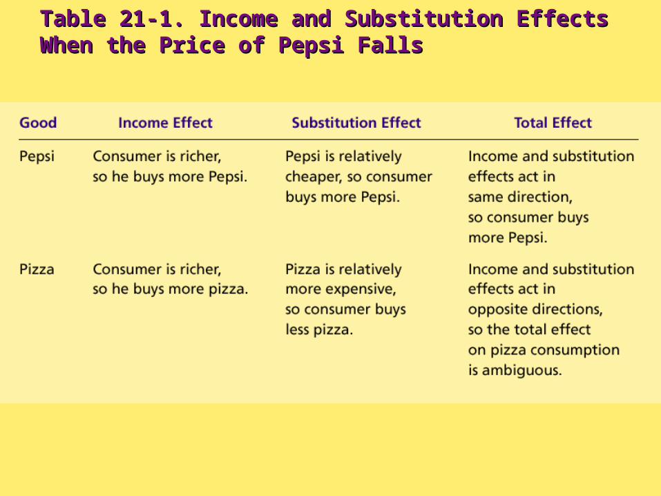
Table 21-1. Income and Substitution Effects When the Table 21-1. Income and Substitution Effects When the Price of Pepsi FallsPrice of Pepsi Falls
Mankiw et al. Principles of Microeconomics, 2nd Canadian Edition Chapter 21: Page 46
Deriving the Demand CurveDeriving the Demand Curve
• A consumer’s demand curve can be viewed as a summary of the optimal decisions that arise from his or her budget constraint and indifference curves.
• A consumer’s demand curve can be viewed as a summary of the optimal decisions that arise from his or her budget constraint and indifference curves.
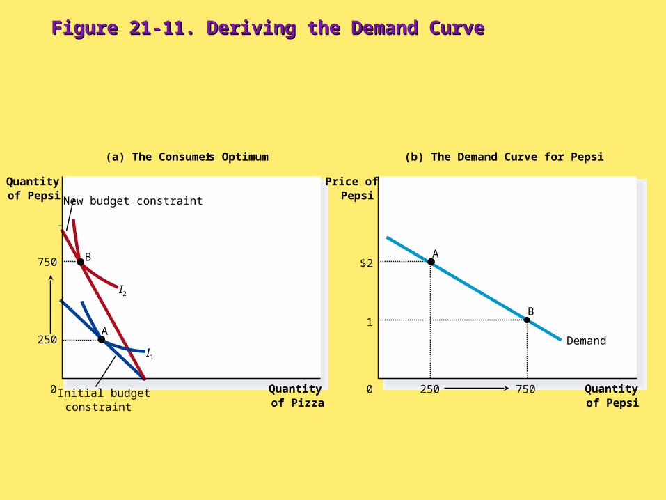
Figure 21-11. Deriving the Demand CurveFigure 21-11. Deriving the Demand Curve
Quantityof Pizza
0
Demand
(a) The Consumer’s Optimum
Quantityof Pepsi
0
Price ofPepsi
(b) The Demand Curve for Pepsi
Quantityof Pepsi
250
$2A
750
1B
I1
I2
New budget constraint
Initial budget constraint
750 B
250A

Mankiw et al. Principles of Microeconomics, 2nd Canadian Edition Chapter 21: Page 48
THREE APPLICATIONSTHREE APPLICATIONS
• Do all demand curves slope downward?– Demand curves can sometimes slope upward.– This happens when a consumer buys more of
a good when its price rises.– Giffen goods
• Economists use the term Giffen good to describe a good that violates the law of demand.
• Giffen goods are goods for which an increase in the price raises the quantity demanded.
• The income effect dominates the substitution effect. • They have demand curves that slope upwards.
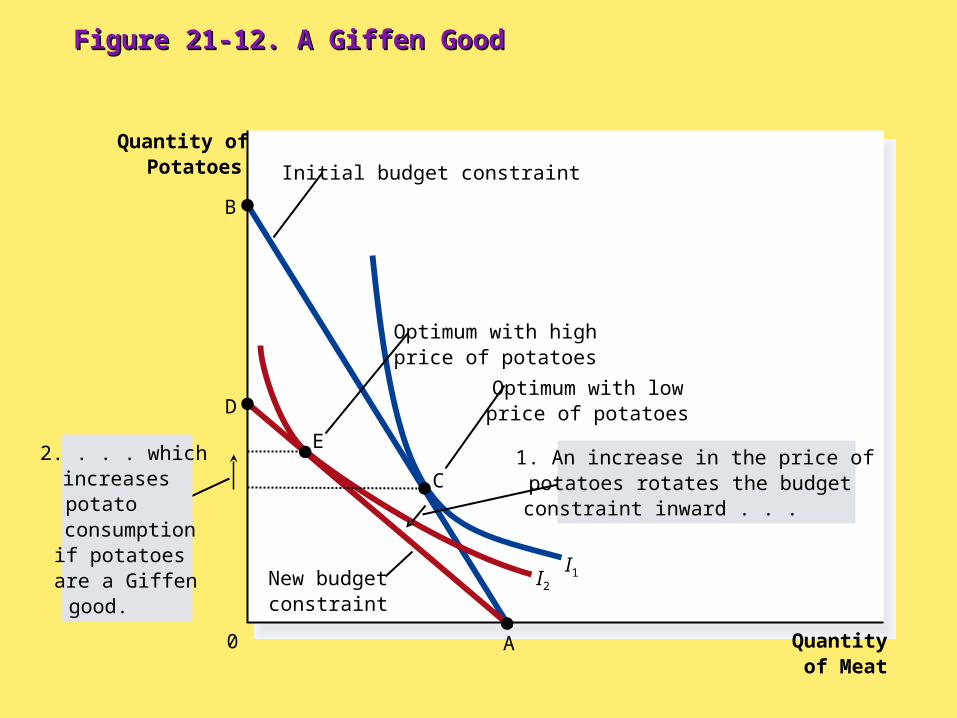
Figure 21-12. A Giffen GoodFigure 21-12. A Giffen Good
Quantityof Meat
Quantity ofPotatoes
0
I2I1
Initial budget constraint
New budgetconstraint
D
A
B
2. . . . which increasespotatoconsumptionif potatoesare a Giffengood.
Optimum with lowprice of potatoes
Optimum with highprice of potatoes
E
C1. An increase in the price ofpotatoes rotates the budgetconstraint inward . . .

Mankiw et al. Principles of Microeconomics, 2nd Canadian Edition Chapter 21: Page 50
THREE APPLICATIONSTHREE APPLICATIONS
• How do wages affect labour supply?– If the substitution effect is greater than
the income effect for the worker, he or she works more.
– If income effect is greater than the substitution effect, he or she works less.
• How do wages affect labour supply?– If the substitution effect is greater than
the income effect for the worker, he or she works more.
– If income effect is greater than the substitution effect, he or she works less.
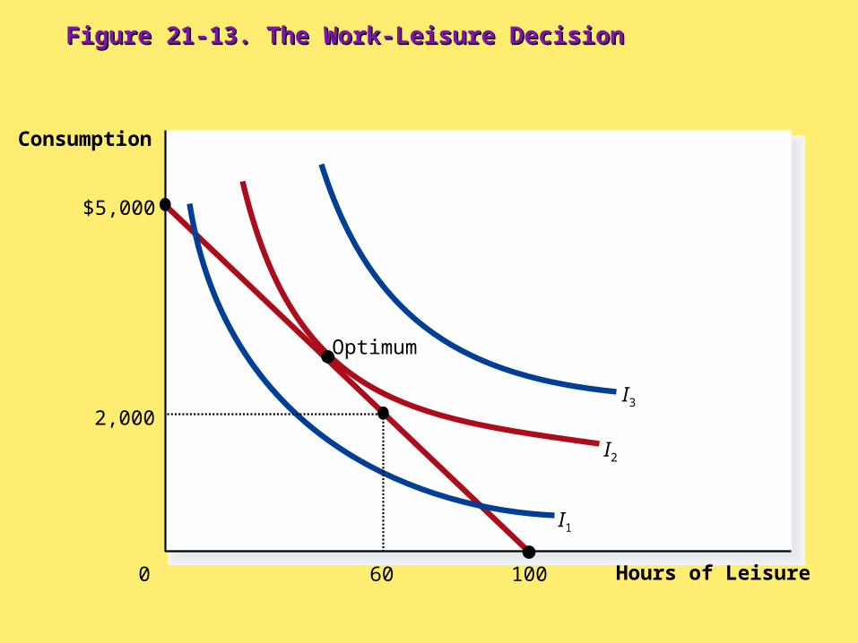
Figure 21-13. The Work-Leisure DecisionFigure 21-13. The Work-Leisure Decision
Hours of Leisure0
Consumption
$5,000
100
I3
I2
I1
Optimum
2,000
60

Figure 21-14. An Increase in the WageFigure 21-14. An Increase in the Wage
Hours ofLeisure
0
Consumption
(a) For a person with these preferences . . .
Hours of labourSupplied
0
Wage
. . . the labour supply curve slopes upward.
I1
I2BC2
BC1
2. . . . hours of leisure decrease . . . 3. . . . and hours of labour increase.
1. When the wage rises . . .
labour supply
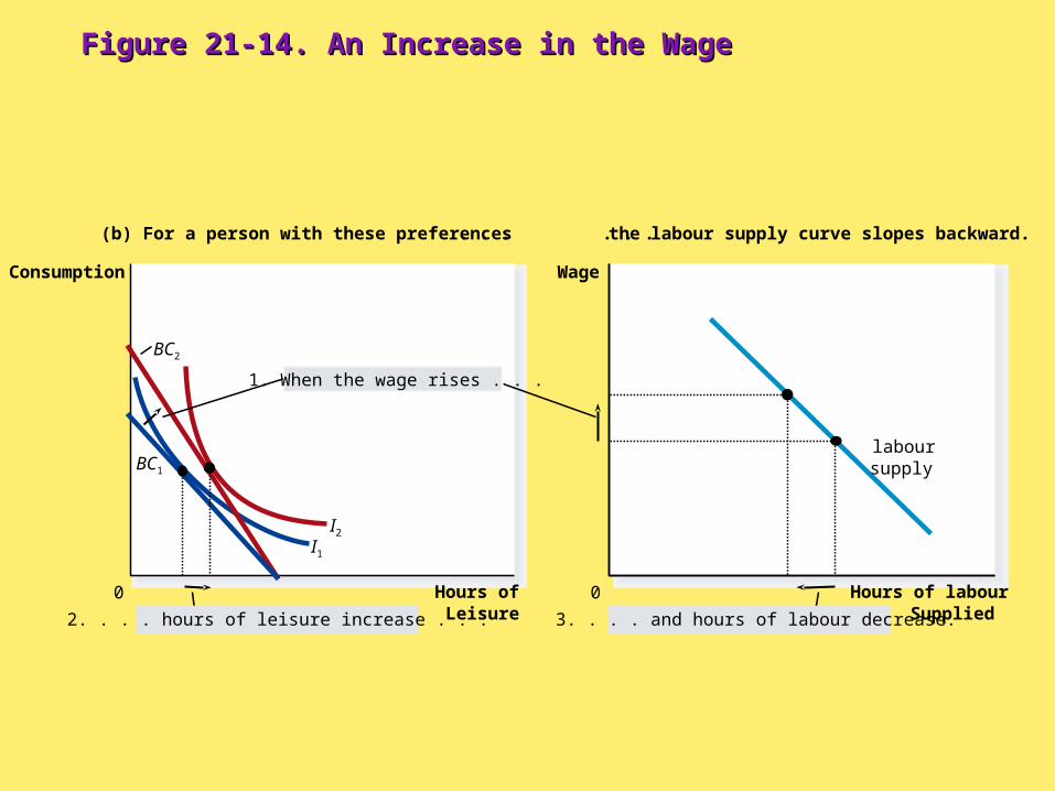
Figure 21-14. An Increase in the WageFigure 21-14. An Increase in the Wage
Hours ofLeisure
0
Consumption
(b) For a person with these preferences . . .
Hours of labourSupplied
0
Wage
. . . the labour supply curve slopes backward.
I1
I2
BC2
BC1
1. When the wage rises . . .
2. . . . hours of leisure increase . . . 3. . . . and hours of labour decrease.
labour supply
Mankiw et al. Principles of Microeconomics, 2nd Canadian Edition Chapter 21: Page 54
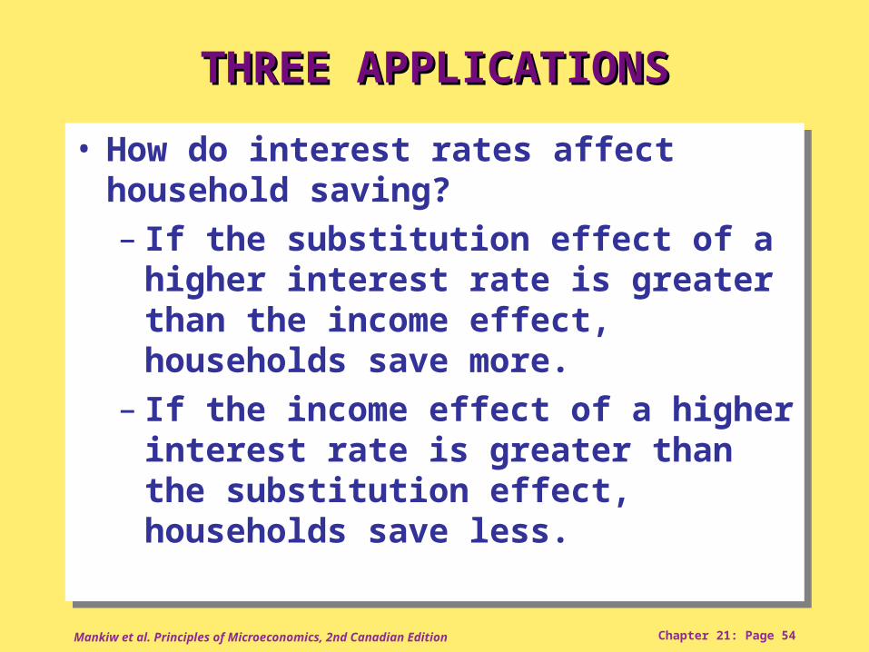
THREE APPLICATIONSTHREE APPLICATIONS
• How do interest rates affect household saving?– If the substitution effect of a higher
interest rate is greater than the income effect, households save more.
– If the income effect of a higher interest rate is greater than the substitution effect, households save less.
• How do interest rates affect household saving?– If the substitution effect of a higher
interest rate is greater than the income effect, households save more.
– If the income effect of a higher interest rate is greater than the substitution effect, households save less.
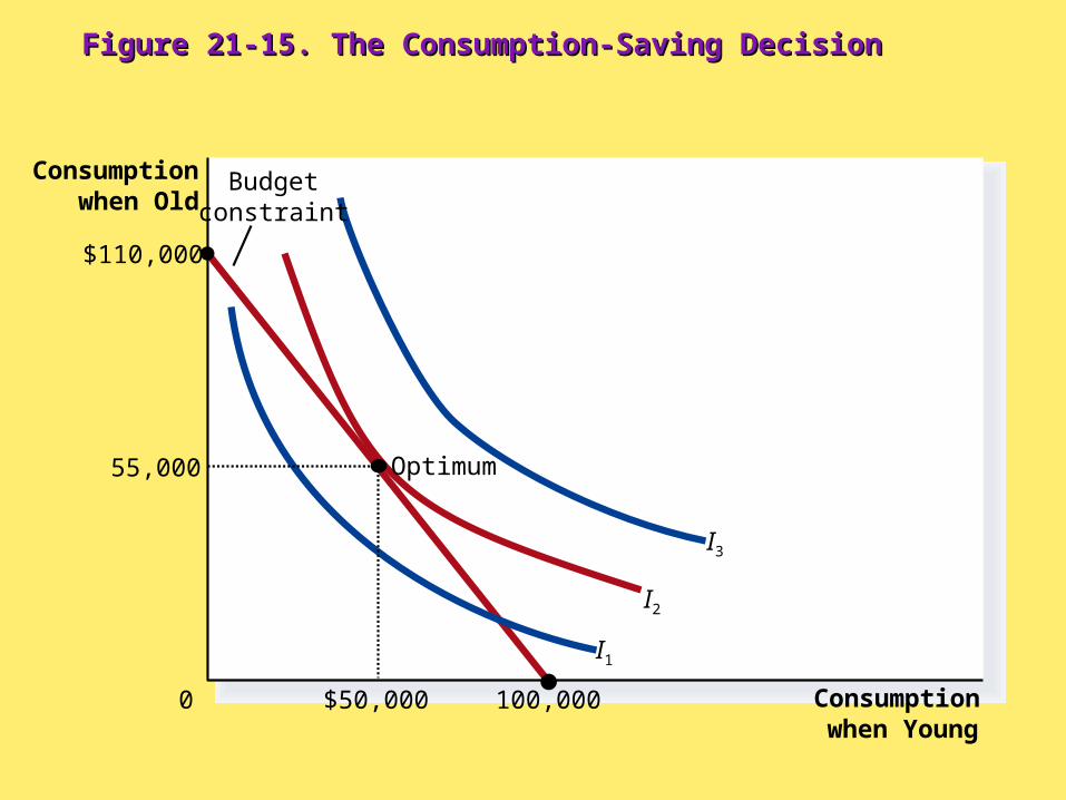
Figure 21-15. The Consumption-Saving DecisionFigure 21-15. The Consumption-Saving Decision
Consumptionwhen Young
0
Consumptionwhen Old
$110,000
100,000
I3
I2
I1
Budgetconstraint
55,000
$50,000
Optimum

Figure 21-16. An Increase in the Interest RateFigure 21-16. An Increase in the Interest Rate
0
(a) Higher Interest Rate Raises Saving (b) Higher Interest Rate Lowers Saving
Consumptionwhen Old
I1
I2
BC1
BC2
0
I1 I2
BC1
BC2
Consumptionwhen Old
Consumptionwhen Young
1. A higher interest rate rotatesthe budget constraint outward . . .
1. A higher interest rate rotatesthe budget constraint outward . . .
2. . . . resulting in lowerconsumption when young and, thus, higher saving.
2. . . . resulting in higherconsumption when youngand, thus, lower saving.
Consumptionwhen Young

Mankiw et al. Principles of Microeconomics, 2nd Canadian Edition Chapter 21: Page 57
THREE APPLICATIONSTHREE APPLICATIONS
• Thus, an increase in the interest rate could either encourage or discourage saving.
• Thus, an increase in the interest rate could either encourage or discourage saving.
Mankiw et al. Principles of Microeconomics, 2nd Canadian Edition Chapter 21: Page 58
SummarySummary
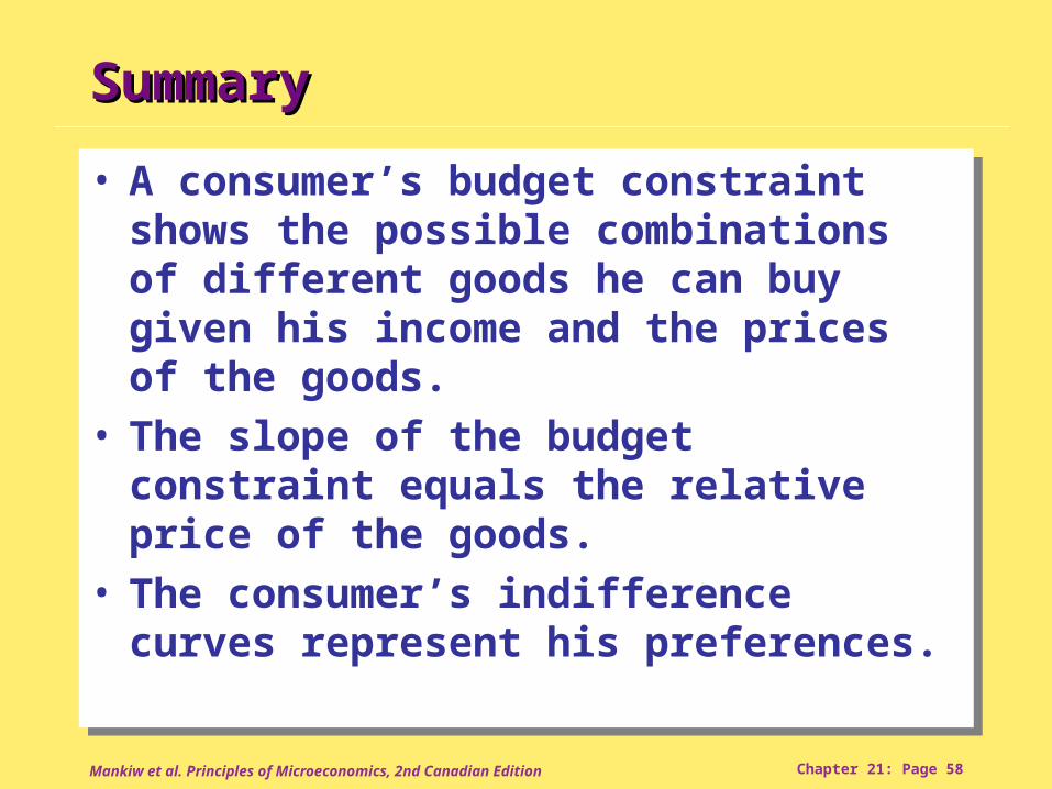
• A consumer’s budget constraint shows the possible combinations of different goods he can buy given his income and the prices of the goods.
• The slope of the budget constraint equals the relative price of the goods.
• The consumer’s indifference curves represent his preferences.
• A consumer’s budget constraint shows the possible combinations of different goods he can buy given his income and the prices of the goods.
• The slope of the budget constraint equals the relative price of the goods.
• The consumer’s indifference curves represent his preferences.
Mankiw et al. Principles of Microeconomics, 2nd Canadian Edition Chapter 21: Page 59
SummarySummary
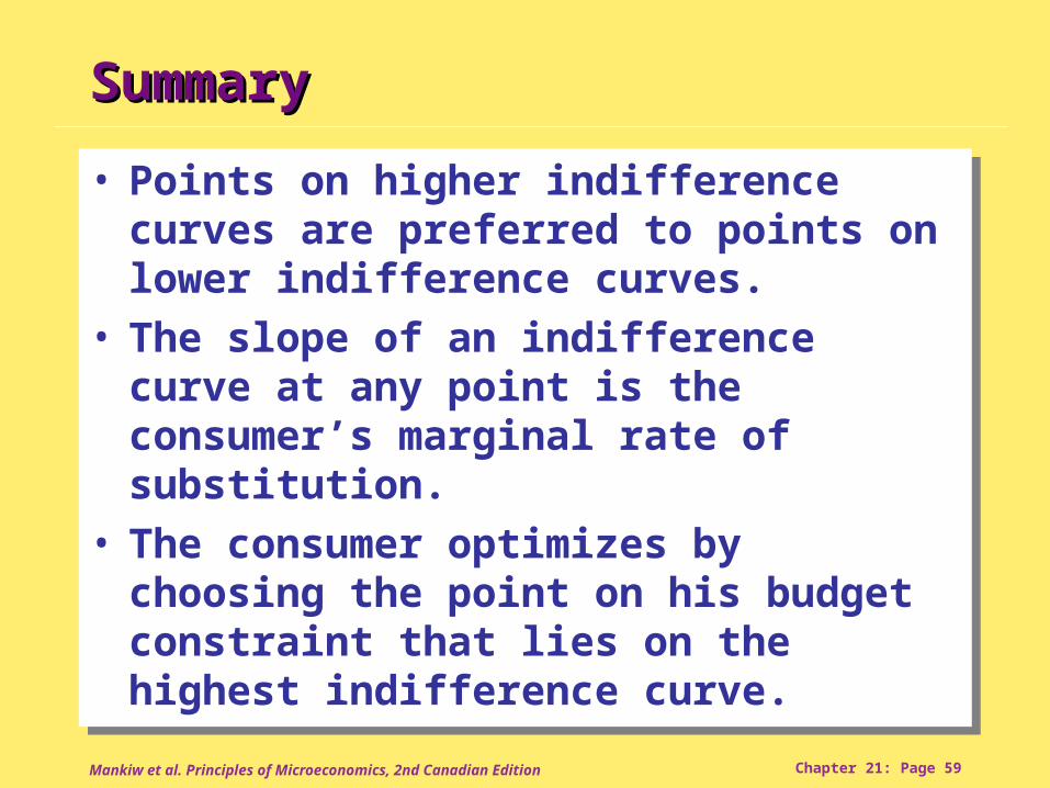
• Points on higher indifference curves are preferred to points on lower indifference curves.
• The slope of an indifference curve at any point is the consumer’s marginal rate of substitution.
• The consumer optimizes by choosing the point on his budget constraint that lies on the highest indifference curve.
Mankiw et al. Principles of Microeconomics, 2nd Canadian Edition Chapter 21: Page 60
SummarySummary
• When the price of a good falls, the impact on the consumer’s choices can be broken down into an income effect and a substitution effect.
• The income effect is the change in consumption that arises because a lower price makes the consumer better off.
• The income effect is reflected by the movement from a lower to a higher indifference curve.
Mankiw et al. Principles of Microeconomics, 2nd Canadian Edition Chapter 21: Page 61
SummarySummary
• The substitution effect is the change in consumption that arises because a price change encourages greater consumption of the good that has become relatively cheaper.
• The substitution effect is reflected by a movement along an indifference curve to a point with a different slope.
• The substitution effect is the change in consumption that arises because a price change encourages greater consumption of the good that has become relatively cheaper.
• The substitution effect is reflected by a movement along an indifference curve to a point with a different slope.
Mankiw et al. Principles of Microeconomics, 2nd Canadian Edition Chapter 21: Page 62
SummarySummary
• The theory of consumer choice can explain:– Why demand curves can potentially
slope upward.– How wages affect labour supply.– How interest rates affect household
saving.
• The theory of consumer choice can explain:– Why demand curves can potentially
slope upward.– How wages affect labour supply.– How interest rates affect household
saving.

Mankiw et al. Principles of Microeconomics, 2nd Canadian Edition Chapter 21: Page 63
The EndThe End


